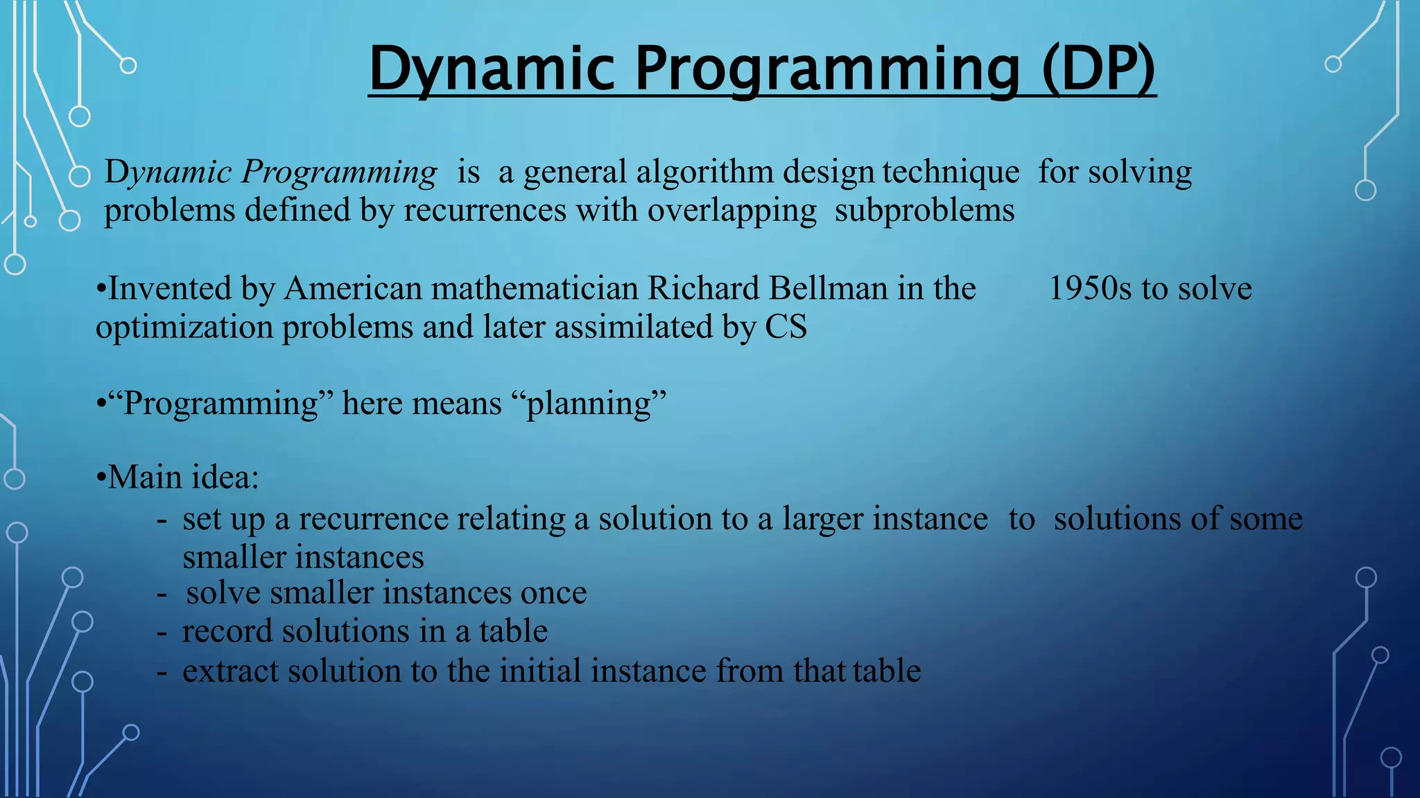
Dynamic programming is an algorithm design technique for solving problems defined by recurrences with overlapping subproblems. It involves breaking down a problem into smaller subproblems, solving each subproblem once, and storing the results for future use. The key aspects are that the optimal solution to a problem relies on the optimal solutions to its subproblems, and that subproblems overlap, allowing for reuse of computed solutions.


![T[i]=min[T[i],1+T[i-coin[j]]]
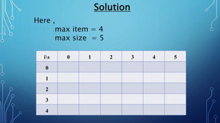
Solution
j c o i n [ j ]
0 8
1 5
2 1
1 2 3 4 5 6 7 8 9 10
1 2 3 4 1 2 3 1 2 2
1 2 3 4 5 6 7 8 9 10
2 2 2 2 1 2 2 0 2 1
10 - 5 = 5 - 5 = 0 5+5=10](https://image.slidesharecdn.com/dynamicprogrammingdp-190909141856/85/Dynamic-programming-dp-in-Algorithm-7-320.jpg)
![is 0 1 2 3 4 5
0 0 0 0 0 0 0
1 0
2 0
3 0
4 0
For s = 0 to s For i = 0
to n
V[0,s] = 0 V[i,0] =
0](https://image.slidesharecdn.com/dynamicprogrammingdp-190909141856/85/Dynamic-programming-dp-in-Algorithm-10-320.jpg)
![is 0 1 2 3 4 5
0 0 0 0 0 0 0
1 0 0
2 0
3 0
4 0
Item (Si,Vi
)
1 (2,3)
2 (3,4)
3 (4,5)
4 (5,6)
If Si<=S
if Vi+V[i-1,S-Si]>V[i-1,S]
V[I,s]=Vi+V[i-1,S-Si]
else
V[I,s]=V[i-1,S]
Else V[I,S]=V[i-1,S]](https://image.slidesharecdn.com/dynamicprogrammingdp-190909141856/85/Dynamic-programming-dp-in-Algorithm-11-320.jpg)
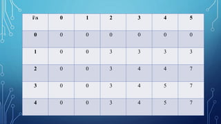
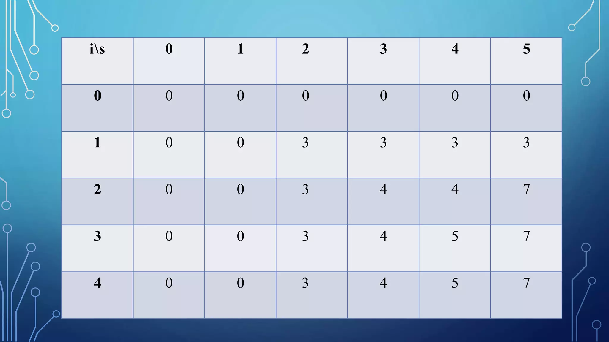
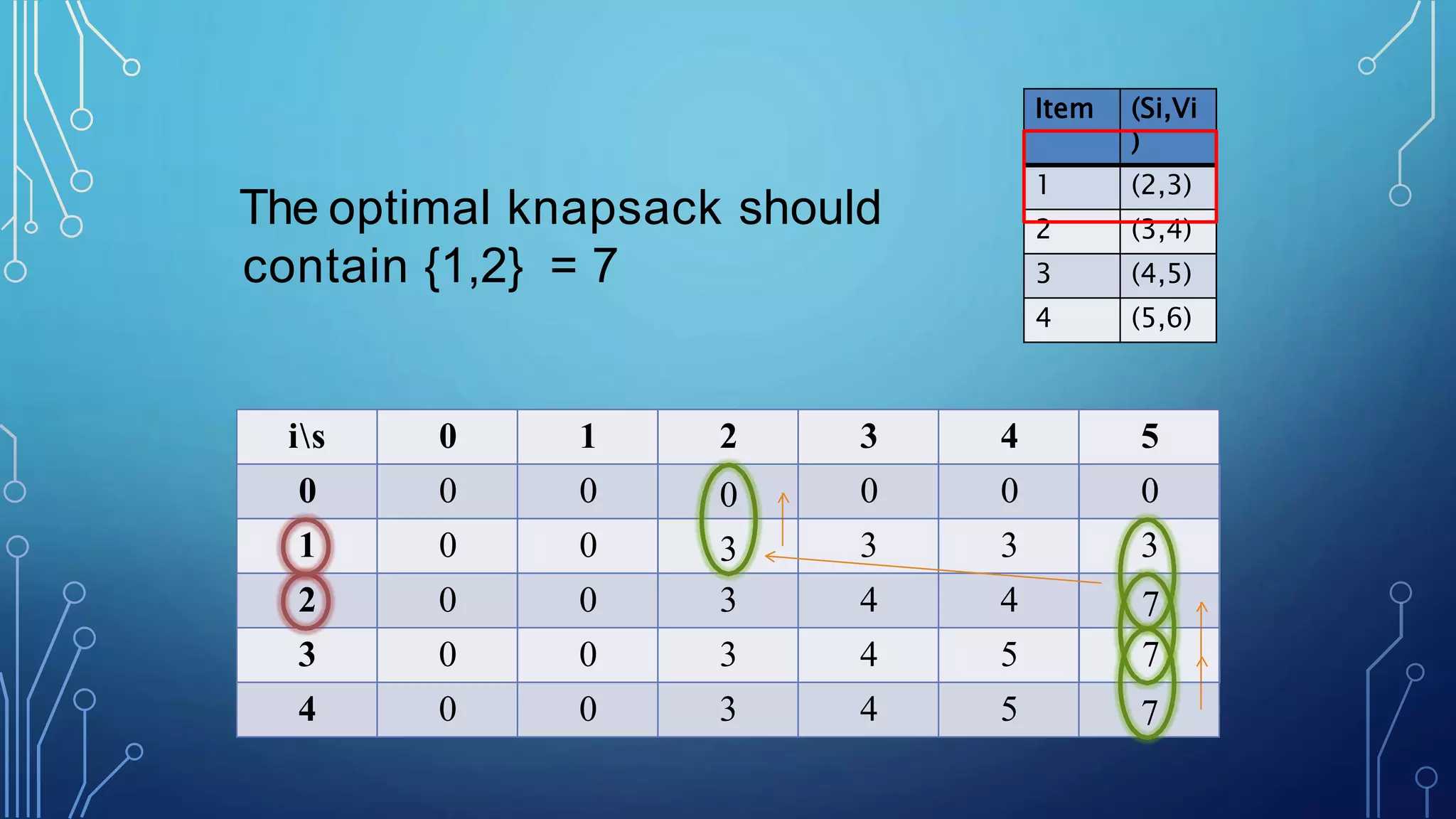
![is 0 1 2 3 4 5
0 0 0 0 0 0 0
1 0 0 3 3 3 3
2 0 0 3 4 4 7
3 0 0 3 4 5 7
4 0 0 3 4 5 7
Item (Si,Vi
)
1 (2,3)
2 (3,4)
3 (4,5)
4 (5,6)
i=n,k=S
while i,k > 0
if V[I,k]=V[1-i,k]
I = i-1, k = k-Si
else
i = i-1](https://image.slidesharecdn.com/dynamicprogrammingdp-190909141856/85/Dynamic-programming-dp-in-Algorithm-13-320.jpg)

![SOLUTION
0 if i = 0 or j = 0
c[i-1, j-1] + 1 if xi = yj
max(c[i, j-1], c[i-1, j]) if xi yj
0 1 2 3 4 5 6
yj B D C A B A
0 0 0 0 0 0 0
0
0
0
0 1 1 1
0 1 1 1
1 2 2
0
1
1 2 2
2
2
0 1
1
2
2 3 3
0
1 2
2
2
3
3
0
1
2
2 3
3 4
0 1
2
2
3 4
4
If xi = yj
b[i, j] = “ ”
Else if
1 xi
2 A
c[i - 1, j] ≥ c[i, j-1] 2 B
3 C
4 B
5 D
6 A
7 B
b[i, j] = “ ”
else
b[i, j] = “ ”
c[i, j] =](https://image.slidesharecdn.com/dynamicprogrammingdp-190909141856/85/Dynamic-programming-dp-in-Algorithm-16-320.jpg)
![• Start at b[m, n] and follow the arrows
• When we encounter a “ “ in b[i, j] xi = yj is an element
of the LCS
1 xi
2 A
3 B
4 C
5 B
6 D
7 A
8 B
0 1 2 3 4 5 6
yj B D C A B A
0 0 0 0 0 0 0
0
0
0
0
0
0
0
0
1
1
1
1
1
1
0
1
1
1
2
2
2
0
1
2
2
2
2
2
1
1
2
2
2
3
3
1
2
2
3
3
3
4
1
2
2
3
3
4
4
Longest common subsequence is {A,B,C,B}](https://image.slidesharecdn.com/dynamicprogrammingdp-190909141856/85/Dynamic-programming-dp-in-Algorithm-17-320.jpg)


![T[i]=min[T[i],1+T[i-coin[j]]]
Solution
j c o i n [ j ]
0 8
1 5
2 1
1 2 3 4 5 6 7 8 9 10
1 2 3 4 1 2 3 1 2 2
1 2 3 4 5 6 7 8 9 10
2 2 2 2 1 2 2 0 2 1
10 - 5 = 5 - 5 = 0 5+5=10](https://image.slidesharecdn.com/dynamicprogrammingdp-190909141856/75/Dynamic-programming-dp-in-Algorithm-7-2048.jpg)

![is 0 1 2 3 4 5
0 0 0 0 0 0 0
1 0
2 0
3 0
4 0
For s = 0 to s For i = 0
to n
V[0,s] = 0 V[i,0] =
0](https://image.slidesharecdn.com/dynamicprogrammingdp-190909141856/75/Dynamic-programming-dp-in-Algorithm-10-2048.jpg)
![is 0 1 2 3 4 5
0 0 0 0 0 0 0
1 0 0
2 0
3 0
4 0
Item (Si,Vi
)
1 (2,3)
2 (3,4)
3 (4,5)
4 (5,6)
If Si<=S
if Vi+V[i-1,S-Si]>V[i-1,S]
V[I,s]=Vi+V[i-1,S-Si]
else
V[I,s]=V[i-1,S]
Else V[I,S]=V[i-1,S]](https://image.slidesharecdn.com/dynamicprogrammingdp-190909141856/75/Dynamic-programming-dp-in-Algorithm-11-2048.jpg)
![is 0 1 2 3 4 5
0 0 0 0 0 0 0
1 0 0 3 3 3 3
2 0 0 3 4 4 7
3 0 0 3 4 5 7
4 0 0 3 4 5 7
Item (Si,Vi
)
1 (2,3)
2 (3,4)
3 (4,5)
4 (5,6)
i=n,k=S
while i,k > 0
if V[I,k]=V[1-i,k]
I = i-1, k = k-Si
else
i = i-1](https://image.slidesharecdn.com/dynamicprogrammingdp-190909141856/75/Dynamic-programming-dp-in-Algorithm-13-2048.jpg)
![SOLUTION
0 if i = 0 or j = 0
c[i-1, j-1] + 1 if xi = yj
max(c[i, j-1], c[i-1, j]) if xi yj
0 1 2 3 4 5 6
yj B D C A B A
0 0 0 0 0 0 0
0
0
0
0 1 1 1
0 1 1 1
1 2 2
0
1
1 2 2
2
2
0 1
1
2
2 3 3
0
1 2
2
2
3
3
0
1
2
2 3
3 4
0 1
2
2
3 4
4
If xi = yj
b[i, j] = “ ”
Else if
1 xi
2 A
c[i - 1, j] ≥ c[i, j-1] 2 B
3 C
4 B
5 D
6 A
7 B
b[i, j] = “ ”
else
b[i, j] = “ ”
c[i, j] =](https://image.slidesharecdn.com/dynamicprogrammingdp-190909141856/75/Dynamic-programming-dp-in-Algorithm-16-2048.jpg)
![• Start at b[m, n] and follow the arrows
• When we encounter a “ “ in b[i, j] xi = yj is an element
of the LCS
1 xi
2 A
3 B
4 C
5 B
6 D
7 A
8 B
0 1 2 3 4 5 6
yj B D C A B A
0 0 0 0 0 0 0
0
0
0
0
0
0
0
0
1
1
1
1
1
1
0
1
1
1
2
2
2
0
1
2
2
2
2
2
1
1
2
2
2
3
3
1
2
2
3
3
3
4
1
2
2
3
3
4
4
Longest common subsequence is {A,B,C,B}](https://image.slidesharecdn.com/dynamicprogrammingdp-190909141856/75/Dynamic-programming-dp-in-Algorithm-17-2048.jpg)