Download to read offline


![# Fitting model
fitControl <- trainControl( method = "repeatedcv", number = 4, repeats = 4)
fit <- train(y ~ ., data = x, method = "gbm", trControl = fitControl,verbose = FAL
SE)
predicted= predict(fit,x_test,type= "prob")[,2]
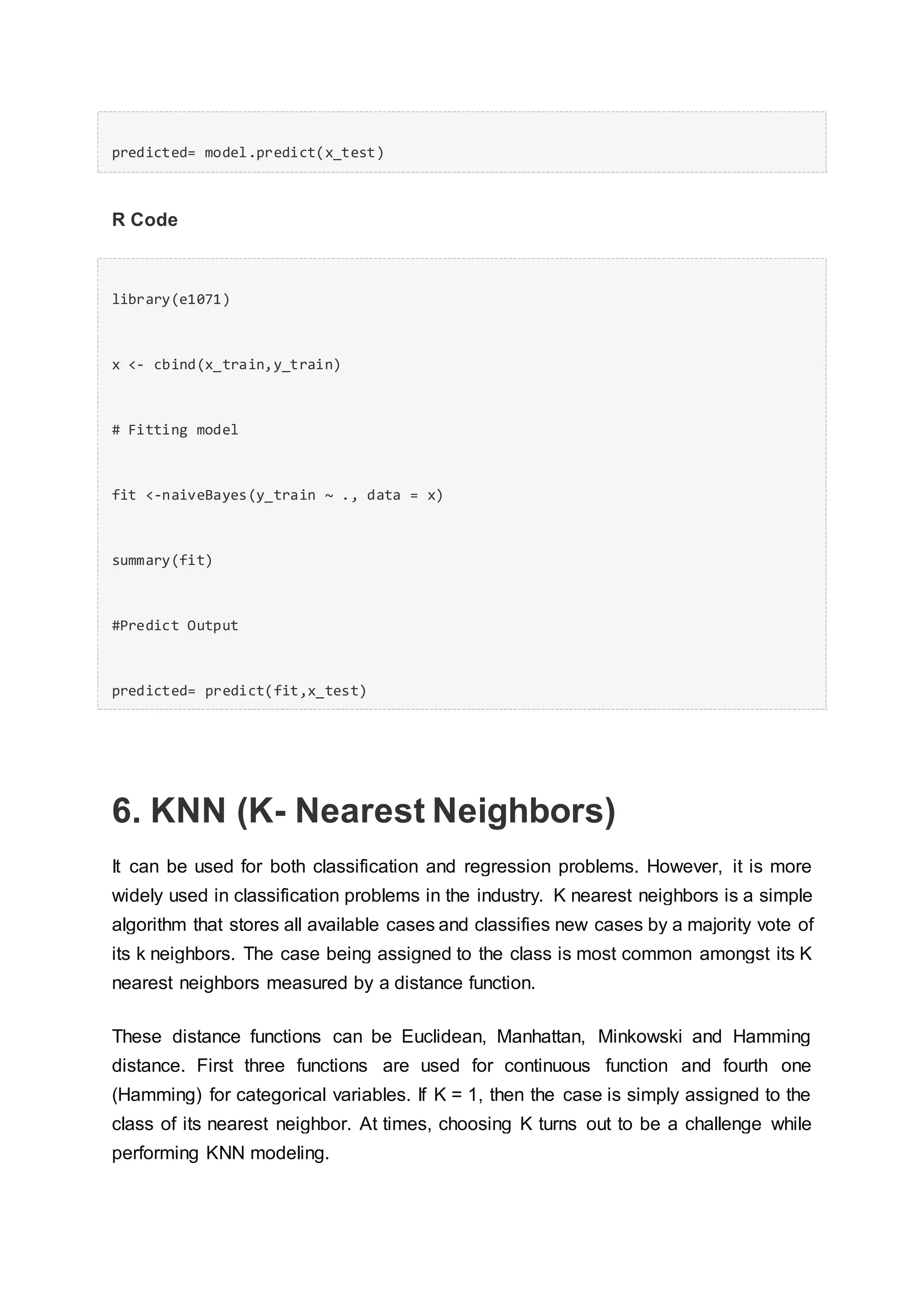
GradientBoostingClassifier and Random Forest are two different boosting tree
classifier and often people ask about the difference between these two algorithms.
End Notes
By now, I am sure, you would have an idea of commonly used machine learning
algorithms. My sole intention behind writing this article and providing the codes in R
and Python is to get you started right away. If you are keen to master machine
learning, start right away. Take up problems, develop a physical understanding of
the process, apply these codes and see the fun!
Did you find this article useful ? Share your views and opinions in the comments
section below.](https://image.slidesharecdn.com/essentialsofmachinelearningalgorithms-160829100013/85/Essentials-of-machine-learning-algorithms-28-320.jpg)


![# Fitting model
fitControl <- trainControl( method = "repeatedcv", number = 4, repeats = 4)
fit <- train(y ~ ., data = x, method = "gbm", trControl = fitControl,verbose = FAL
SE)
predicted= predict(fit,x_test,type= "prob")[,2]
GradientBoostingClassifier and Random Forest are two different boosting tree
classifier and often people ask about the difference between these two algorithms.
End Notes
By now, I am sure, you would have an idea of commonly used machine learning
algorithms. My sole intention behind writing this article and providing the codes in R
and Python is to get you started right away. If you are keen to master machine
learning, start right away. Take up problems, develop a physical understanding of
the process, apply these codes and see the fun!
Did you find this article useful ? Share your views and opinions in the comments
section below.](https://image.slidesharecdn.com/essentialsofmachinelearningalgorithms-160829100013/75/Essentials-of-machine-learning-algorithms-28-2048.jpg)

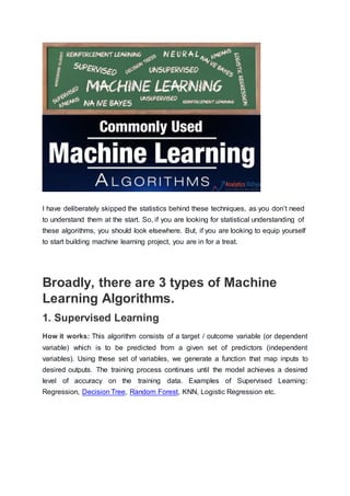
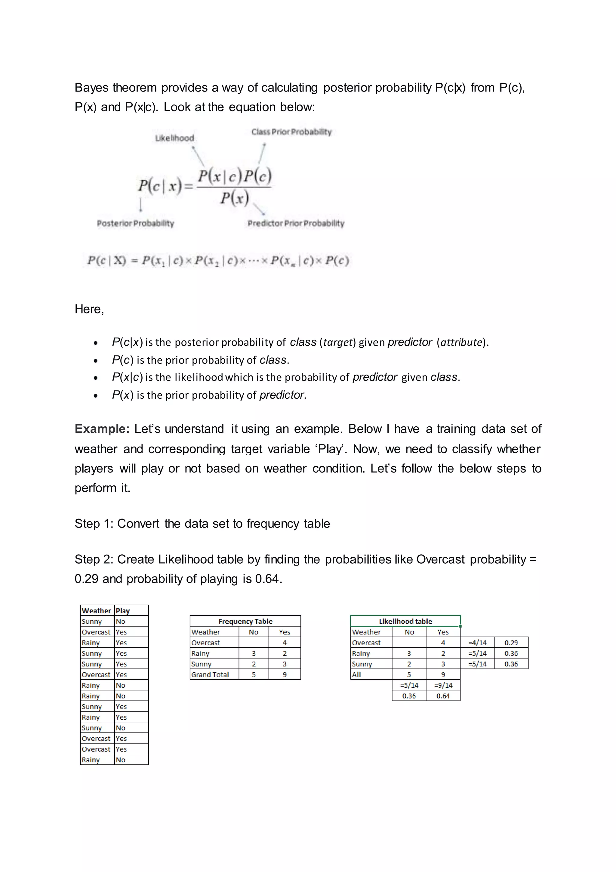
This document provides an introduction and overview of machine learning algorithms. It begins by discussing the importance and growth of machine learning. It then describes the three main types of machine learning algorithms: supervised learning, unsupervised learning, and reinforcement learning. Next, it lists and briefly defines ten commonly used machine learning algorithms including linear regression, logistic regression, decision trees, SVM, Naive Bayes, and KNN. For each algorithm, it provides a simplified example to illustrate how it works along with sample Python and R code.


![Matrix and determinant URT [Autosaved].pptx](https://cdn.slidesharecdn.com/ss_thumbnails/matrixanddeterminanturtautosaved-251018190340-9e6a6deb-thumbnail.jpg?width=600ounds&width=560&fit=bounds)


