Downloaded 15 times


![Applications
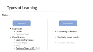
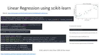
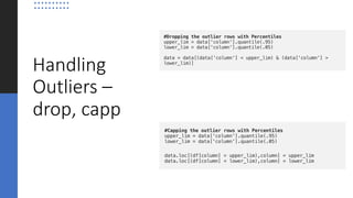
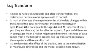
• Trendline --- A trend line represents a trend, the long-term movement in time series data after other
components have been accounted for. It tells whether a particular data set (say GDP, oil prices or stock prices) have
increased or decreased over the period of time.
• Epidemiology --- Early evidence relating tobacco smoking to mortality and morbidity came from observational
studies employing regression analysis. In order to reduce spurious correlations when analyzing observational data,
researchers usually include several variables in their regression models in addition to the variable of primary interest.
• Finance --- The capital asset pricing model uses linear regression as well as the concept of beta for analyzing and
quantifying the systematic risk of an investment. This comes directly from the beta coefficient of the linear regression
model that relates the return on the investment to the return on all risky assets.
• Economics --- Linear regression is the predominant empirical tool in economics. For example, it is used to
predict consumption spending,[20] fixed investment spending, inventory investment, purchases of a
country's exports,[21] spending on imports,[21] the demand to hold liquid assets,[22] labor demand,[23] and labor
supply.[23]
https://en.wikipedia.org/wiki/Linear_regression](https://image.slidesharecdn.com/introtoml-200626174707/85/Introduction-to-machine-learning-12-320.jpg)
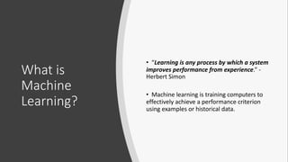
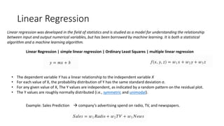
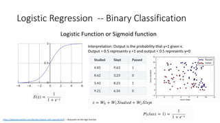
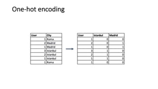
![Classification
http://cs229.stanford.edu/notes2020spring/cs229-notes1.pdf
Values of Y, i.e the response can take discrete values
o Binary Classification – response can belong to two
classes (0,1)
üRating – thumbs up, thumbs down.
o Multi-class classification – there can be n classes à
[1, …. n]
ü Movie/restaurant rating can range from
[1,2,3,4,5]
o Multi-class , multi – label classification.
üExample –
ØConcept space in Probability has many
concepts (classes) – [Probability, Bayes
Theorem, DiscretePDF – Binomial, Poisson,
Continuous PDF – normal, exponential, …]
ØA question will typically belong to multiple
classes.](https://image.slidesharecdn.com/introtoml-200626174707/85/Introduction-to-machine-learning-13-320.jpg)


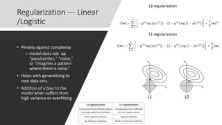


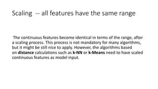


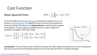
![Applications
• Trendline --- A trend line represents a trend, the long-term movement in time series data after other
components have been accounted for. It tells whether a particular data set (say GDP, oil prices or stock prices) have
increased or decreased over the period of time.
• Epidemiology --- Early evidence relating tobacco smoking to mortality and morbidity came from observational
studies employing regression analysis. In order to reduce spurious correlations when analyzing observational data,
researchers usually include several variables in their regression models in addition to the variable of primary interest.
• Finance --- The capital asset pricing model uses linear regression as well as the concept of beta for analyzing and
quantifying the systematic risk of an investment. This comes directly from the beta coefficient of the linear regression
model that relates the return on the investment to the return on all risky assets.
• Economics --- Linear regression is the predominant empirical tool in economics. For example, it is used to
predict consumption spending,[20] fixed investment spending, inventory investment, purchases of a
country's exports,[21] spending on imports,[21] the demand to hold liquid assets,[22] labor demand,[23] and labor
supply.[23]
https://en.wikipedia.org/wiki/Linear_regression](https://image.slidesharecdn.com/introtoml-200626174707/75/Introduction-to-machine-learning-12-2048.jpg)
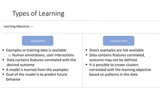
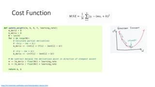
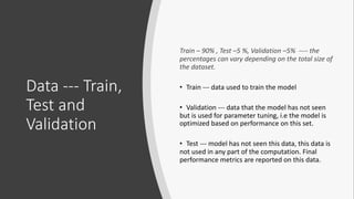
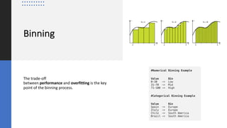
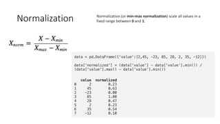
![Classification
http://cs229.stanford.edu/notes2020spring/cs229-notes1.pdf
Values of Y, i.e the response can take discrete values
o Binary Classification – response can belong to two
classes (0,1)
üRating – thumbs up, thumbs down.
o Multi-class classification – there can be n classes à
[1, …. n]
ü Movie/restaurant rating can range from
[1,2,3,4,5]
o Multi-class , multi – label classification.
üExample –
ØConcept space in Probability has many
concepts (classes) – [Probability, Bayes
Theorem, DiscretePDF – Binomial, Poisson,
Continuous PDF – normal, exponential, …]
ØA question will typically belong to multiple
classes.](https://image.slidesharecdn.com/introtoml-200626174707/75/Introduction-to-machine-learning-13-2048.jpg)


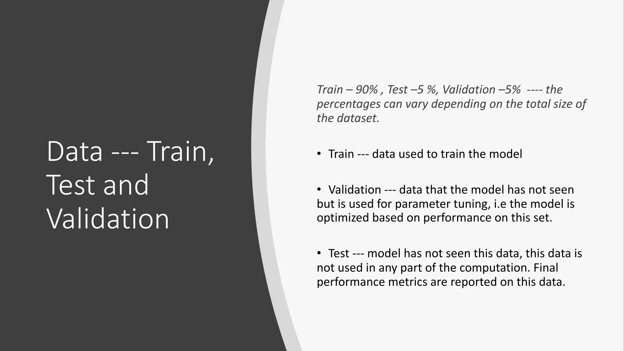


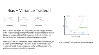
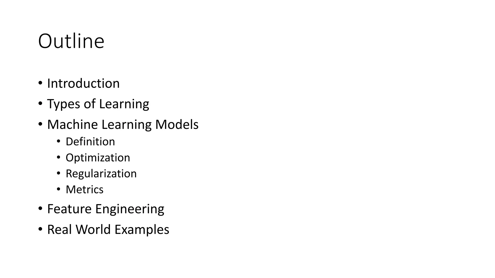
The document provides an introduction to machine learning, covering its definitions, types (supervised and unsupervised learning), models, and applications across various fields such as healthcare, finance, and education. It also delves into specific algorithms like linear regression, decision trees, and clustering methods, highlighting their use cases, advantages, and challenges, along with performance metrics for evaluating models. Additionally, it discusses techniques for feature engineering and optimization methods that enhance model accuracy and efficiency.
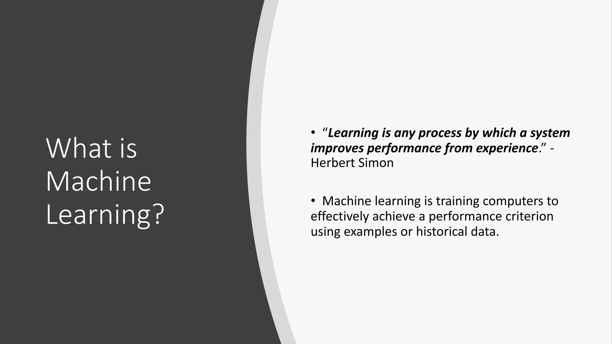
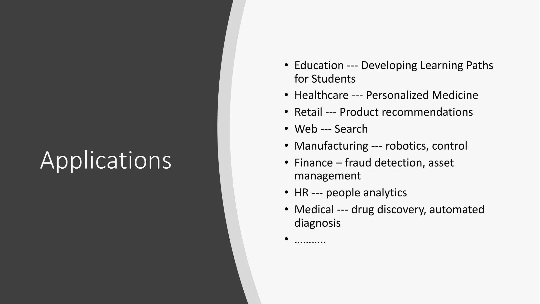
Overview of machine learning; its definition and significance; real-world applications.
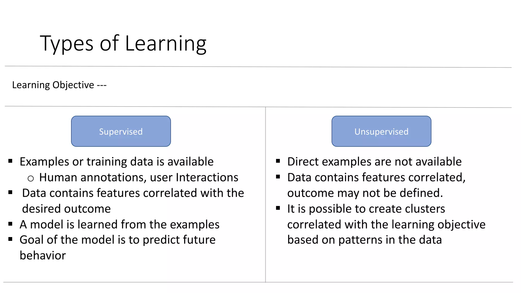
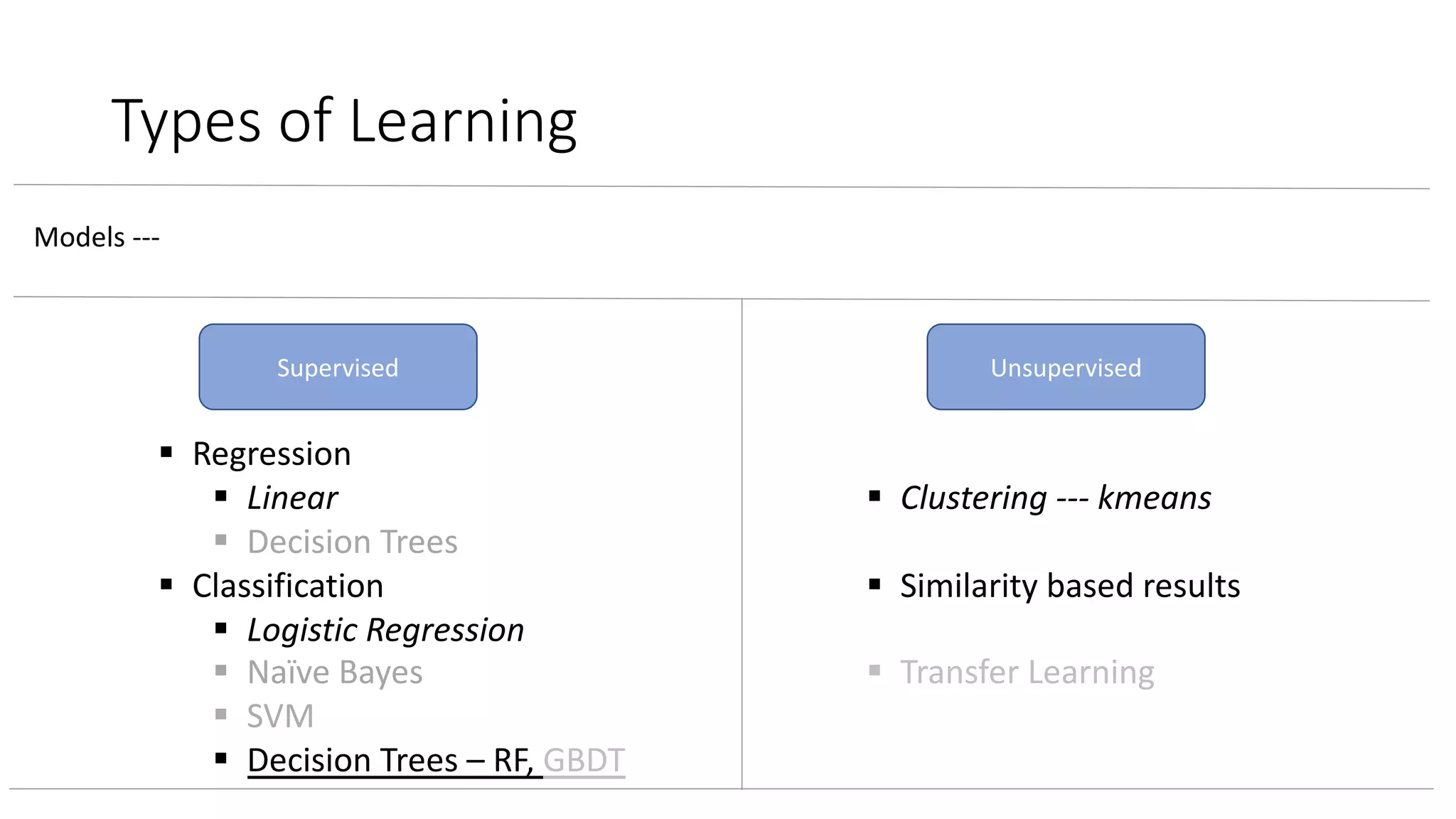
Explains supervised vs. unsupervised learning, including examples and objectives for each type.
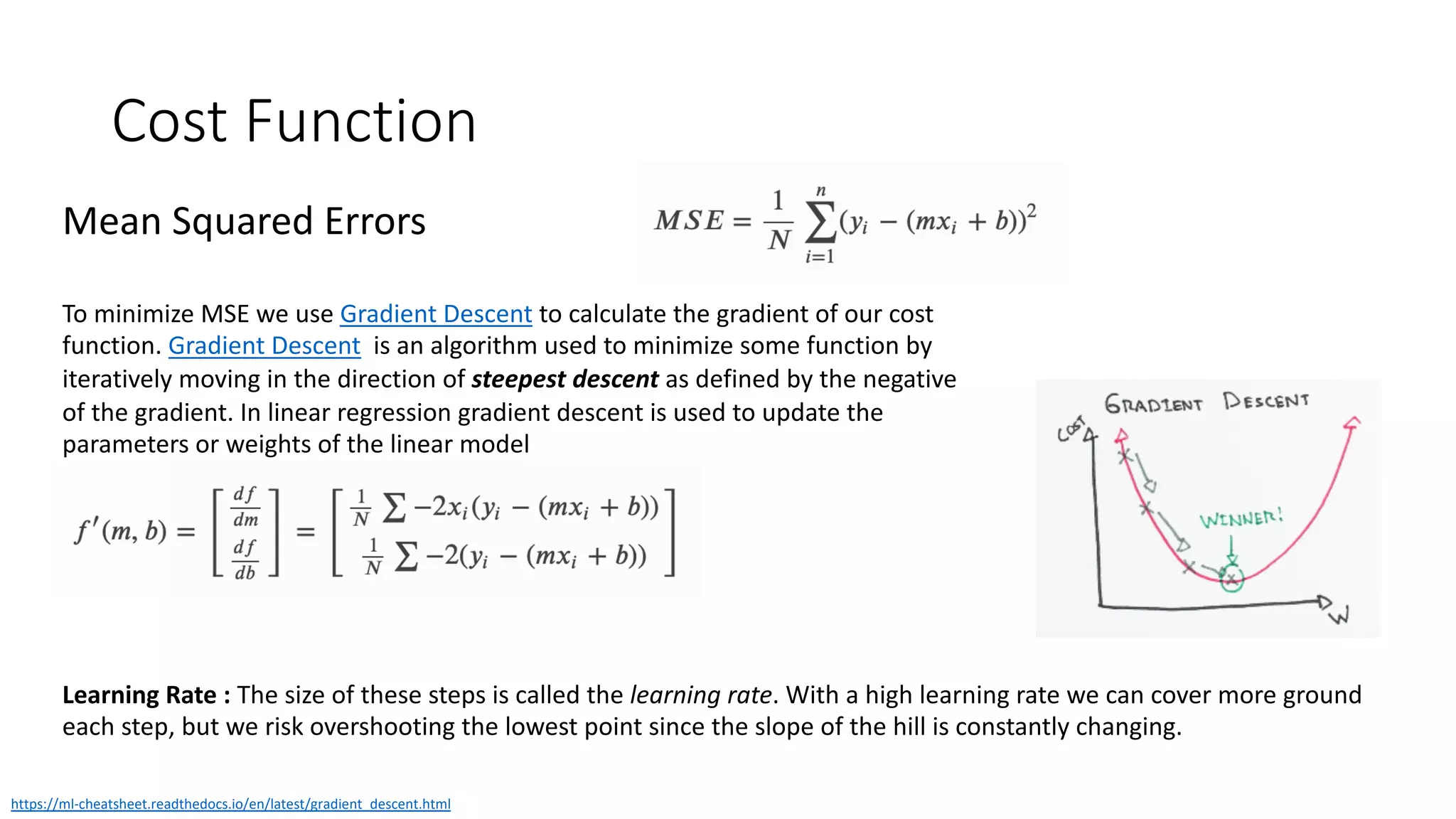
Detailed description of linear regression, its cost function, applications, and classification methods.
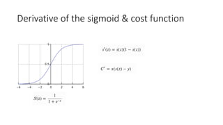
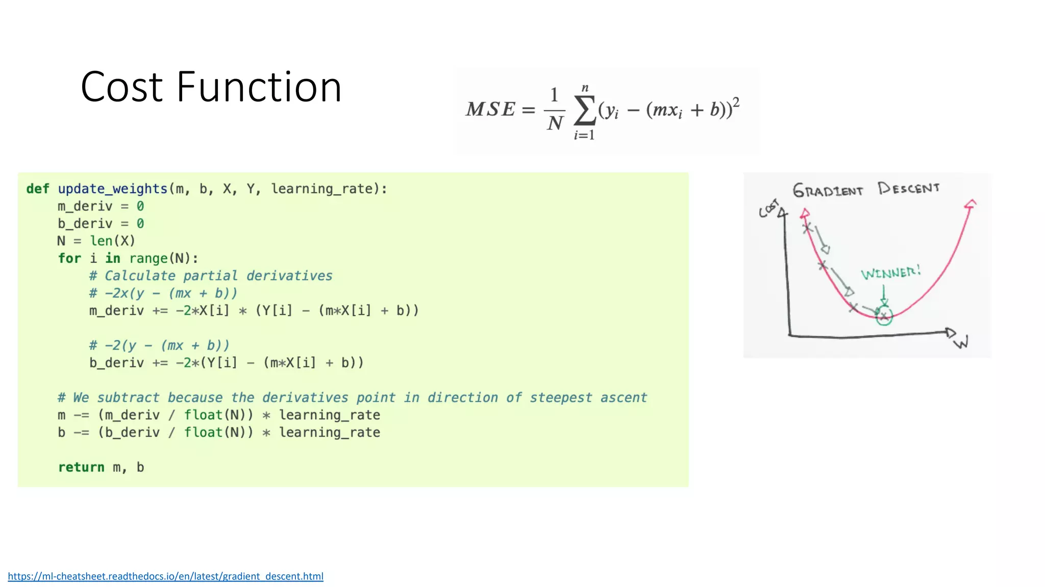
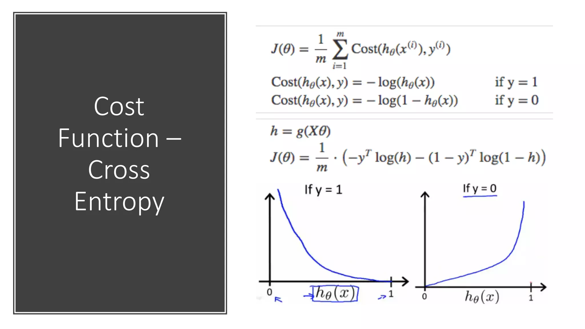
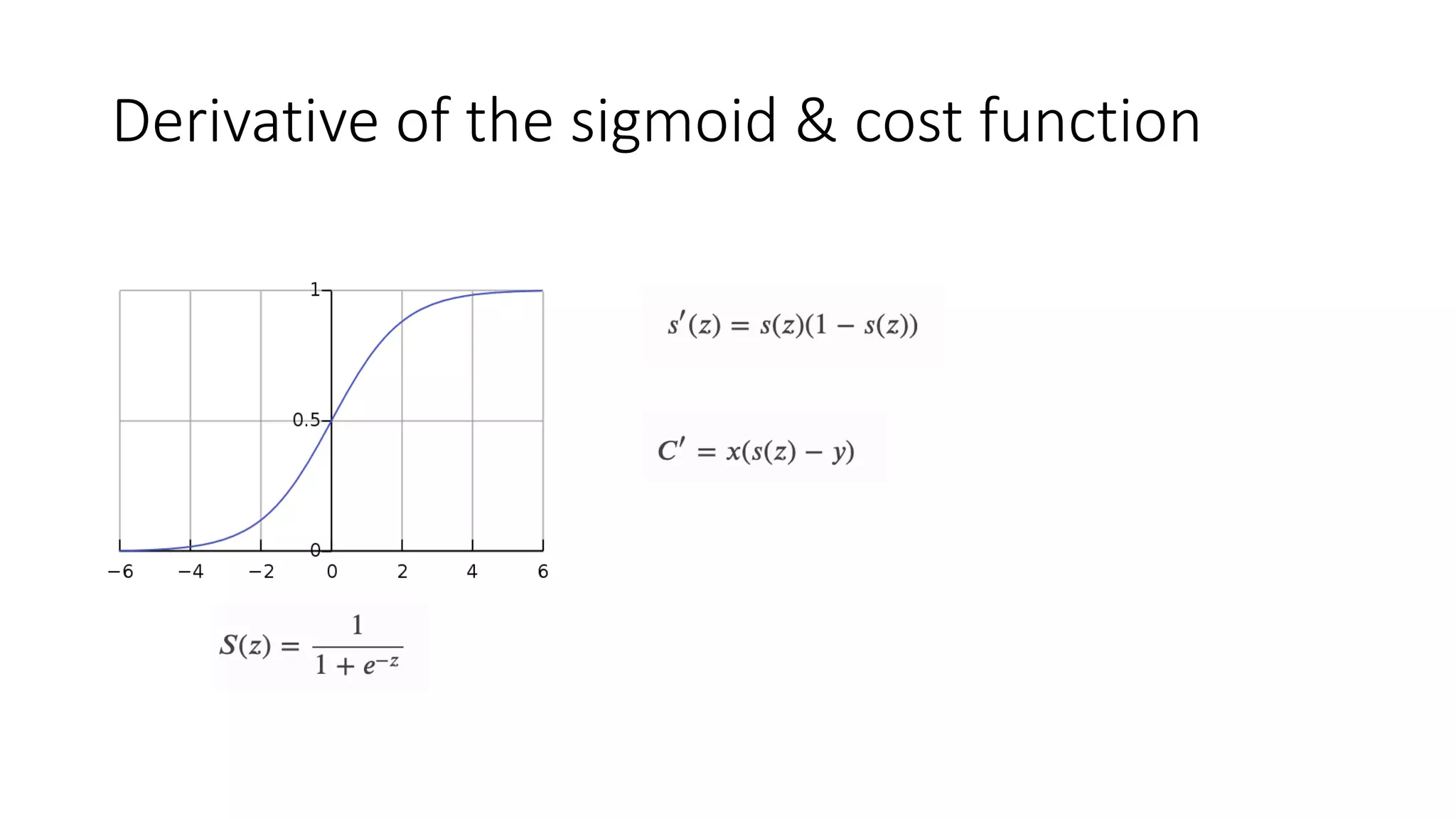
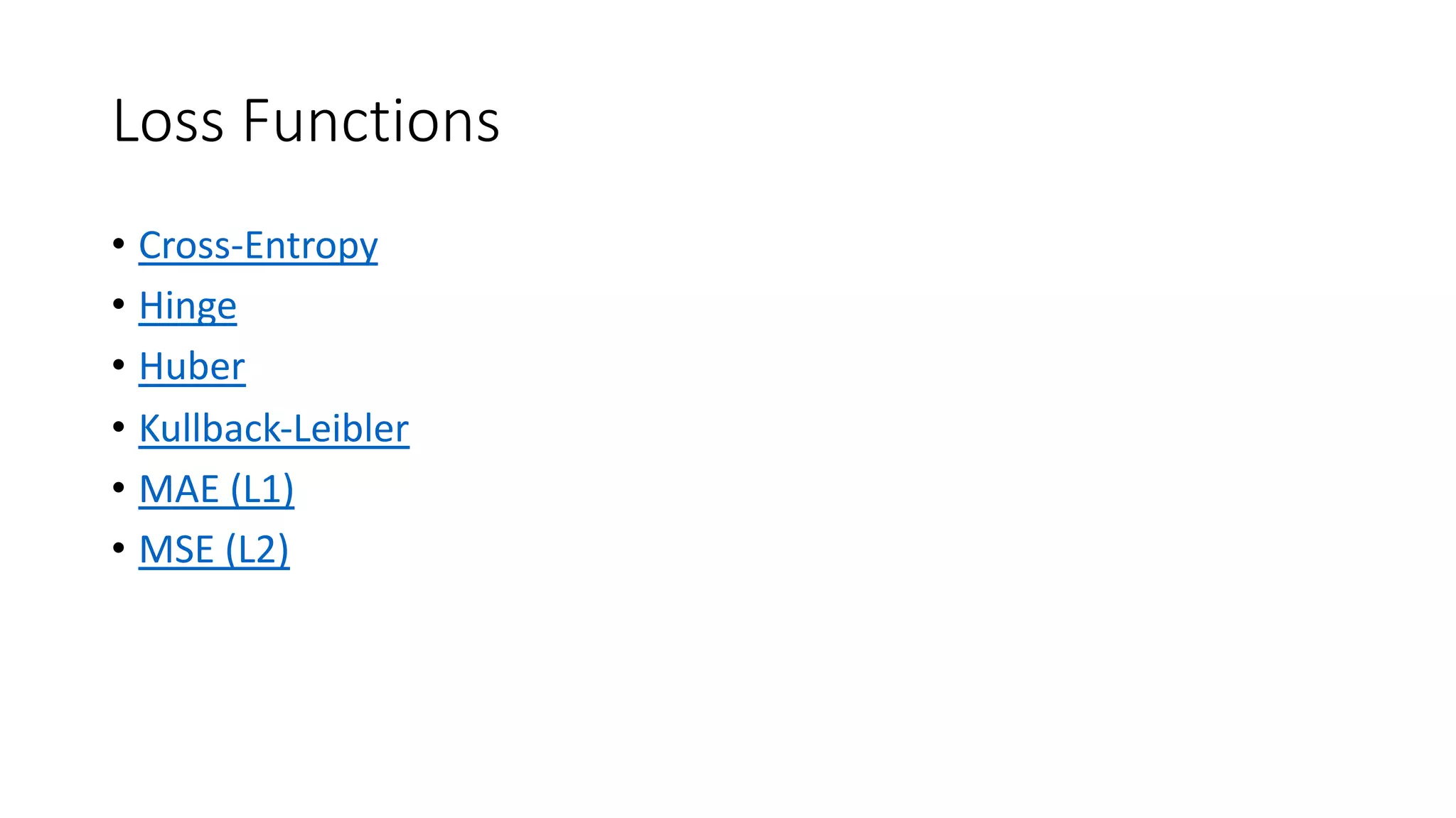
Discussion of cost functions used in machine learning; gradient descent optimization and challenges.
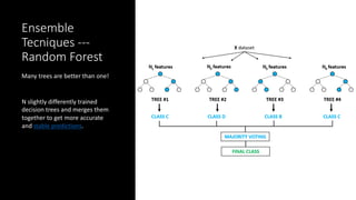
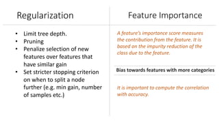
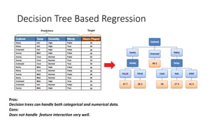
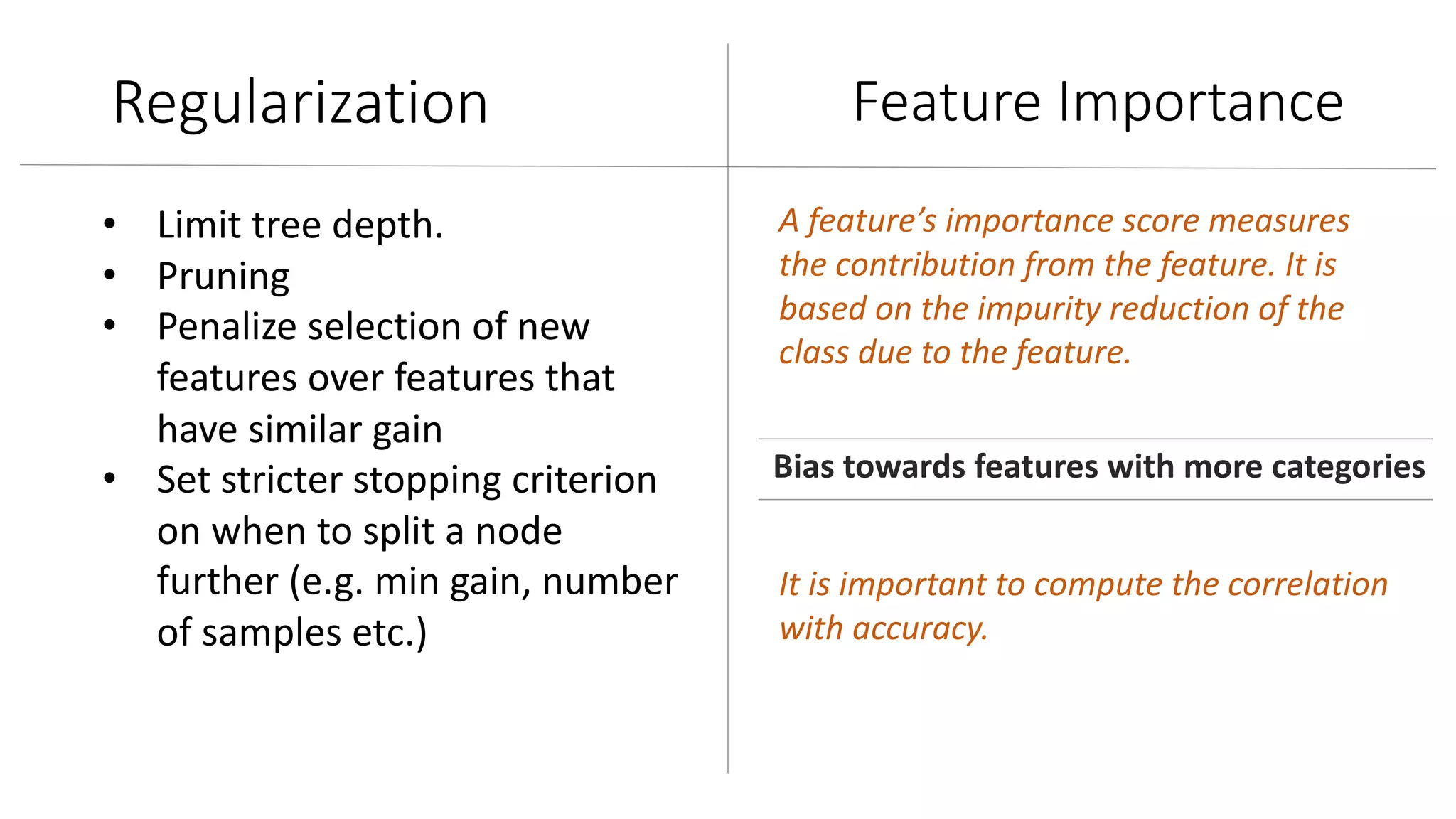
Insights on decision tree modeling, its pros and cons, and the benefits of ensemble techniques like random forests.
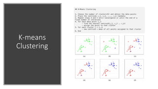
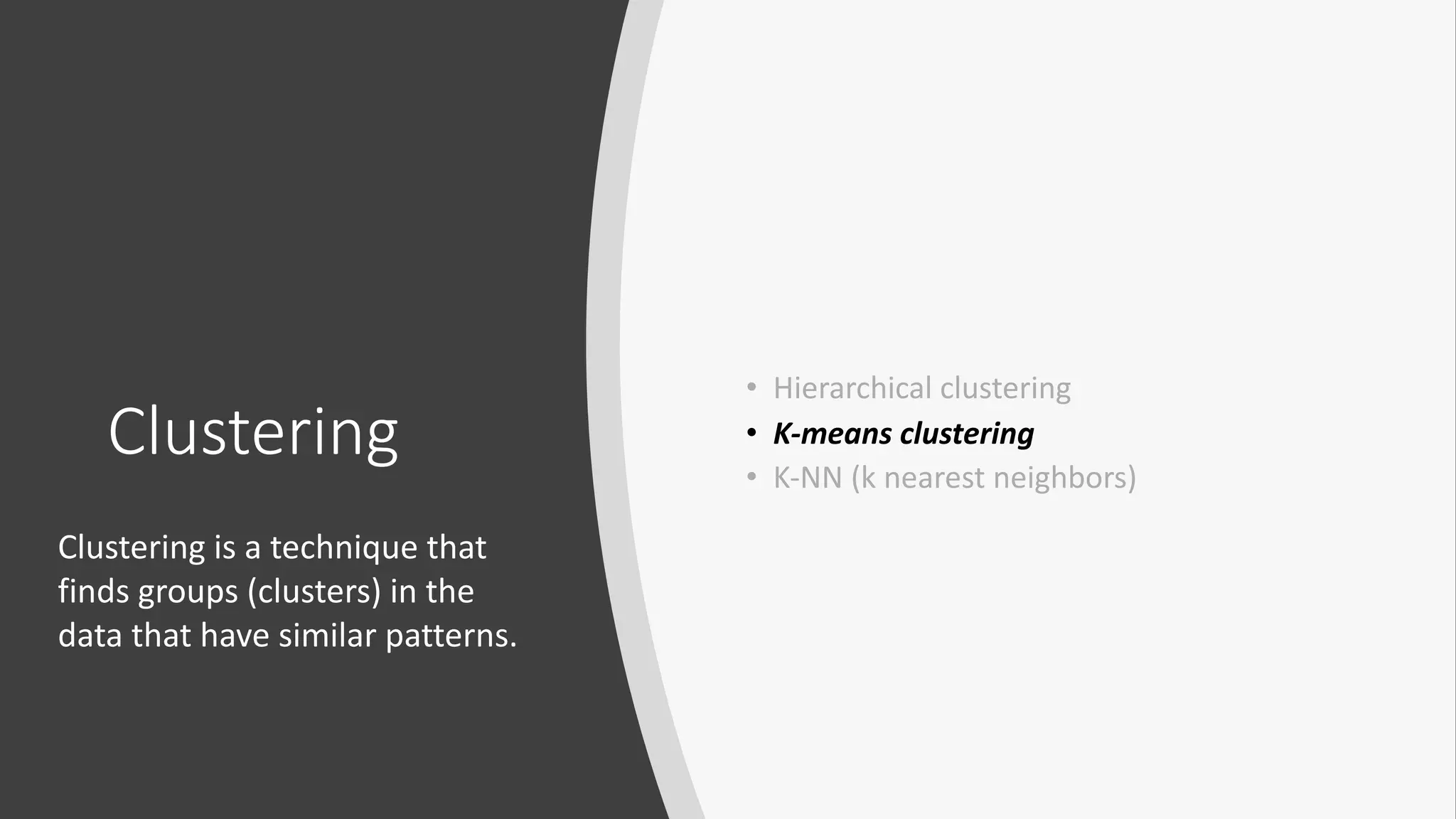
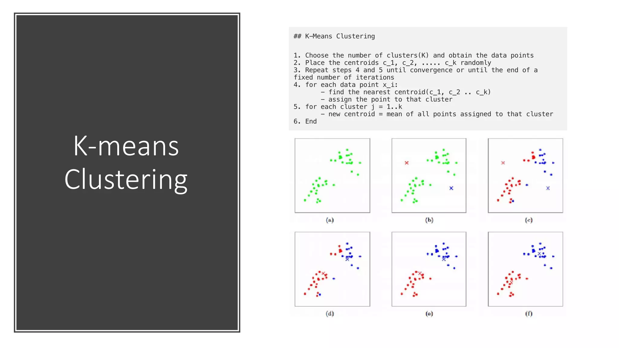
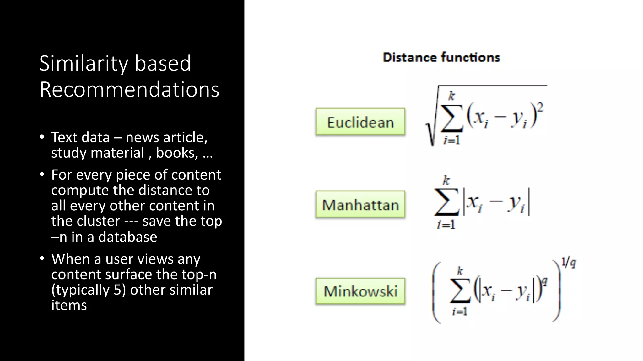
Introduction to unsupervised learning, clustering techniques, and their applications in pattern recognition.
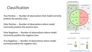
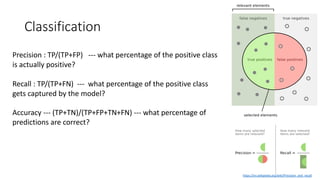
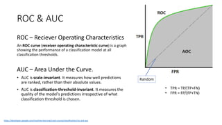
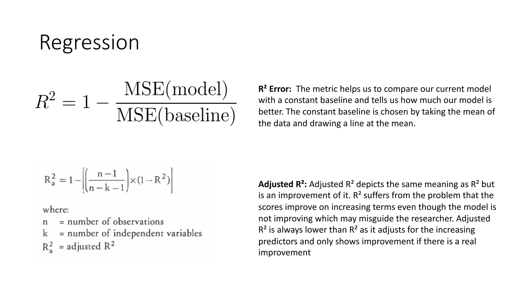
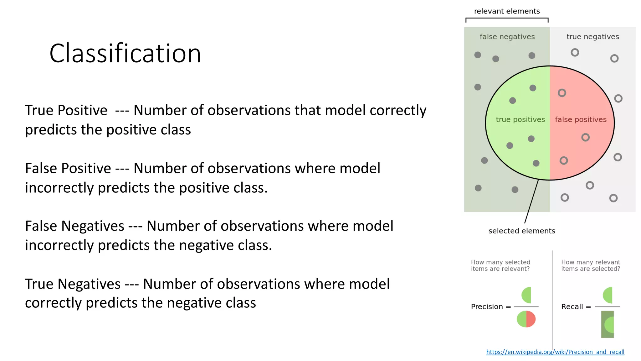
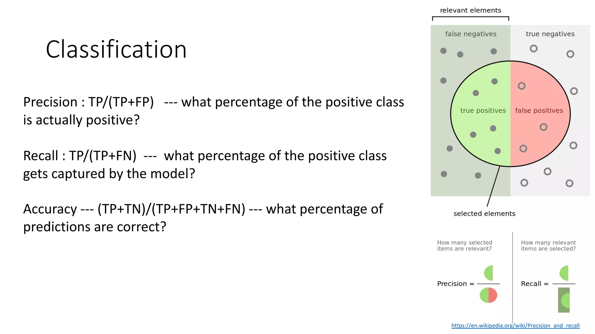
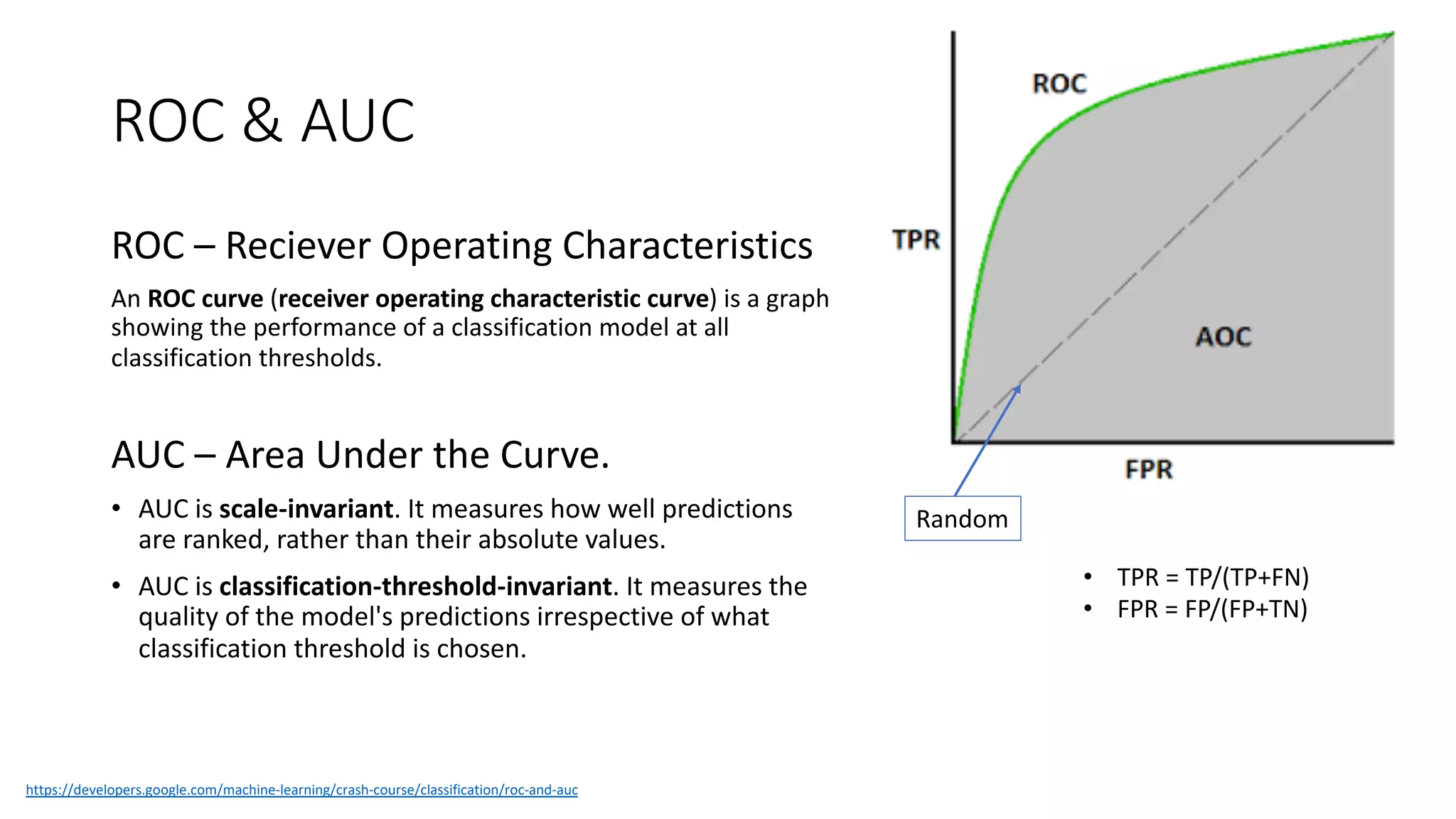
Key performance metrics in regression and classification, including ROC, AUC, precision, and recall.
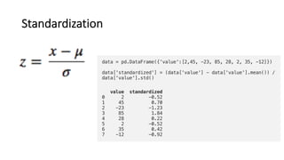
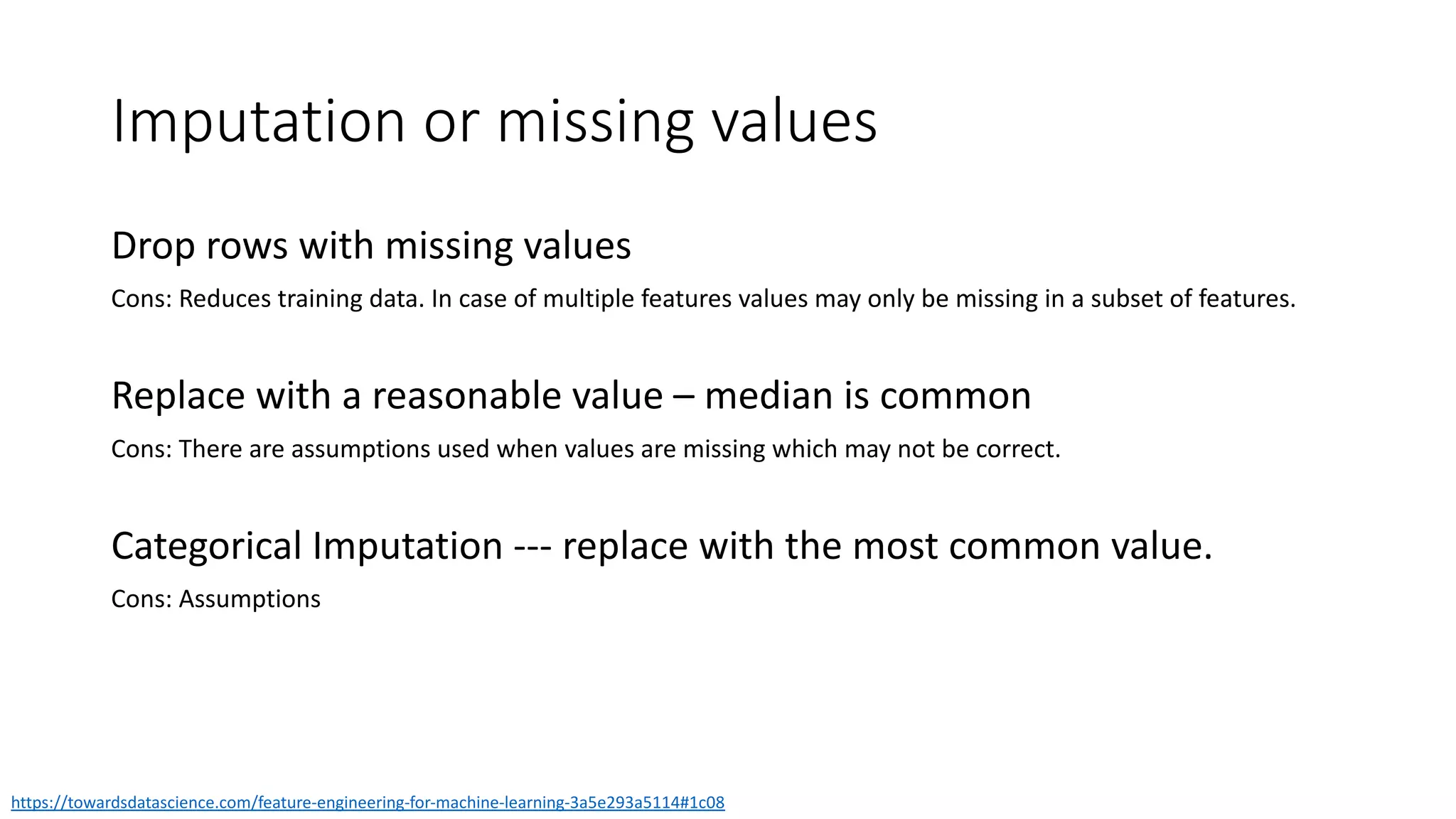
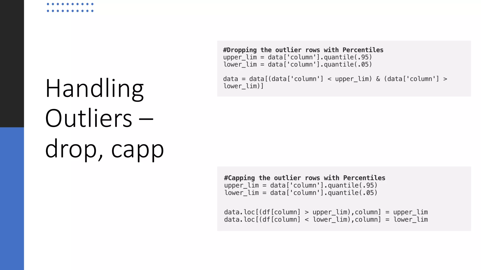
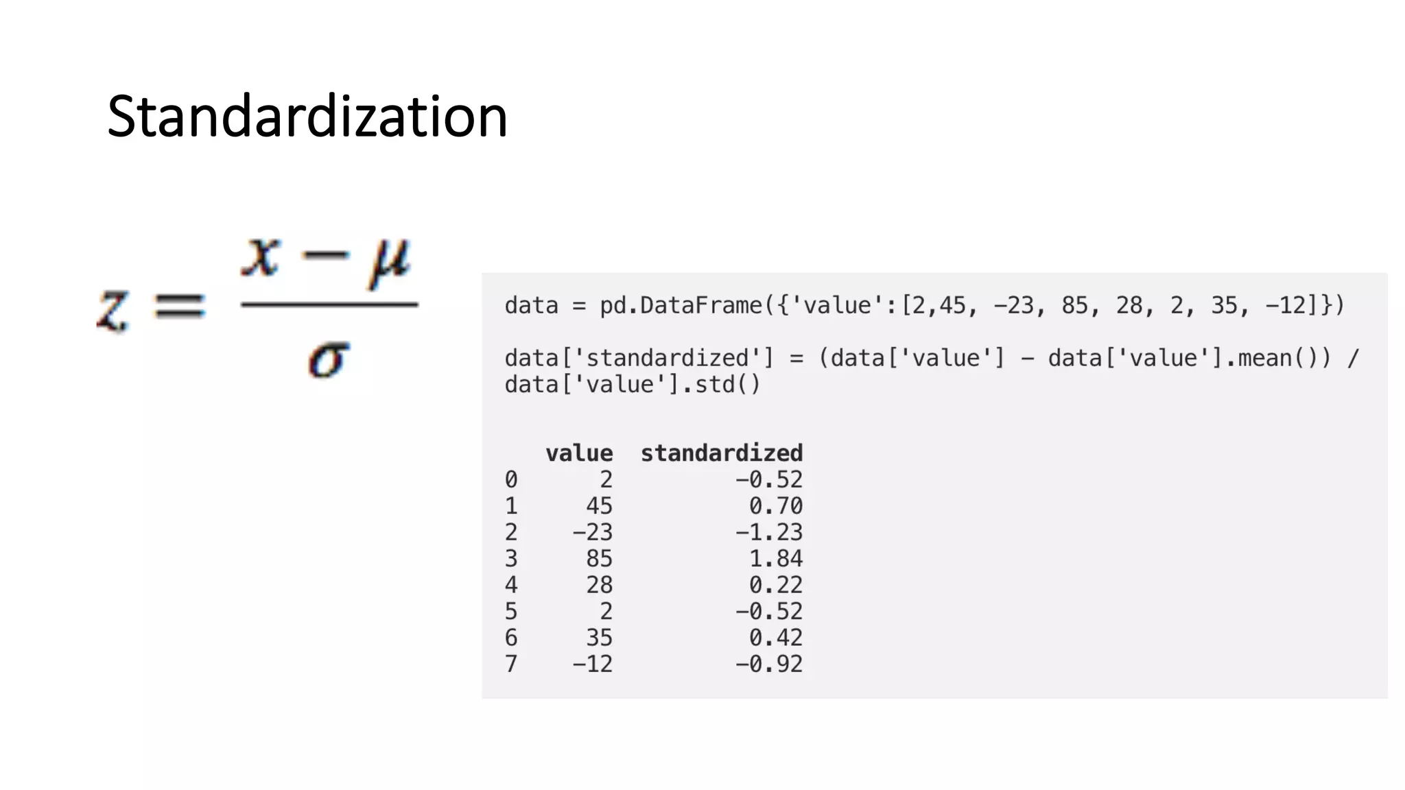
Methods for handling missing values, outliers, and feature scaling approaches important for model performance.
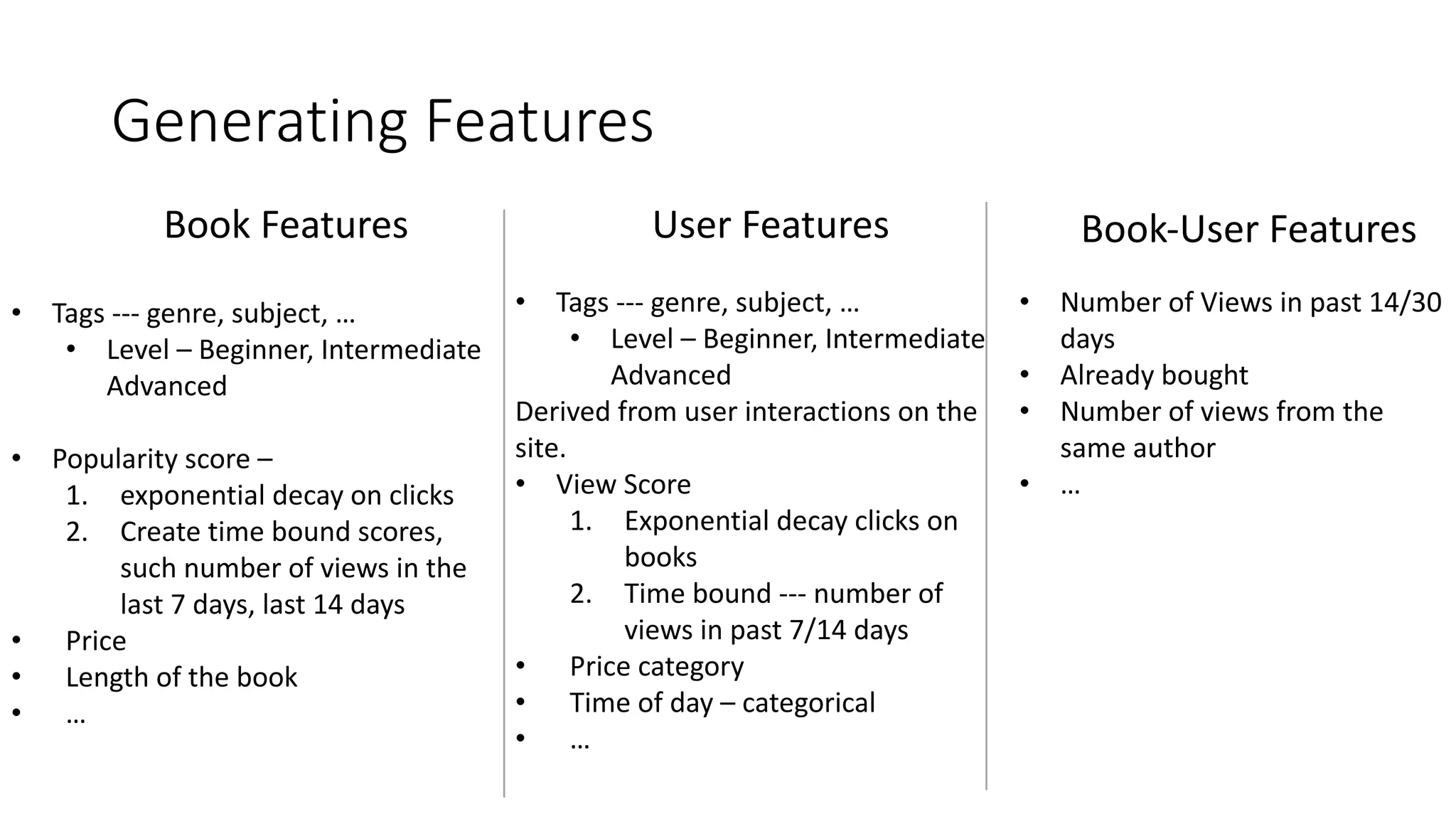
Example use case of a predictive model for user engagement in an online bookstore context.
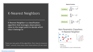
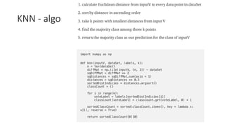
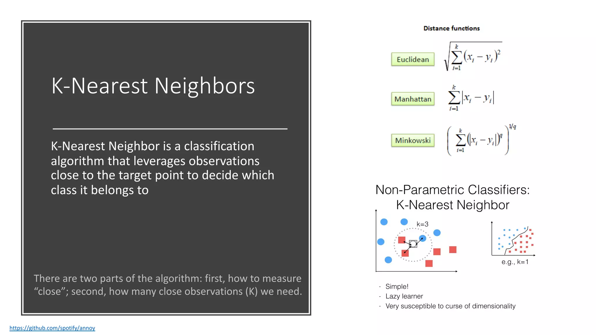
Technical overview of K-Nearest Neighbors, various metrics for ranking, and optimization techniques.


