KEMBAR78
in computer data structures and algorithms | DOCX
DMI-ST. JOHN THE BAPTIST UNIVERSITY
LILONGWE, MALAWI
Module Code: 351CS34
Subject Name: DATA STRUCTURE AND ALGORITHM
Unit I Detail Notes
School of Computer Science
Module Teacher: Fanny Chatola
Syllabus
Introduction to Algorithm and Data Structures:
Algorithms- Problem Solving, Introduction to Algorithms, Characteristics of algorithms, Algorithm design tools:
Pseudo code and flowchart, Analysis of Algorithms, Complexity of algorithms - Space complexity, Time
complexity, Asymptotic notation - Big-O, Theta and Omega, standard measures of efficiency. Data Structures-
Data structure, Abstract Data Types (ADT), Concept of linear and Non-linear, static and dynamic, persistent
and ephemeral data structures, and relationship among data, data structure, and algorithm, From Problem to
Program. Algorithmic Strategies- Introduction to algorithm design strategies - Divide and Conquer, and Greedy
strategy. Recurrence relation - Recurrence Relation, Linear Recurrence Relations, With constant Coefficients,
Homogeneous Solutions. Solving recurrence relations.
TABLE OF CONTENTS
No table of contents entries found.
Problem Solving:
 For finding solution to problems
 It is used in many disciplines
Ex: Problems
1. Sorting
2. Searching
3. String problem
4. Graph problems
5. Combinational problems
6. Geometric problems
7. Numerical problems
Introduction to algorithms:
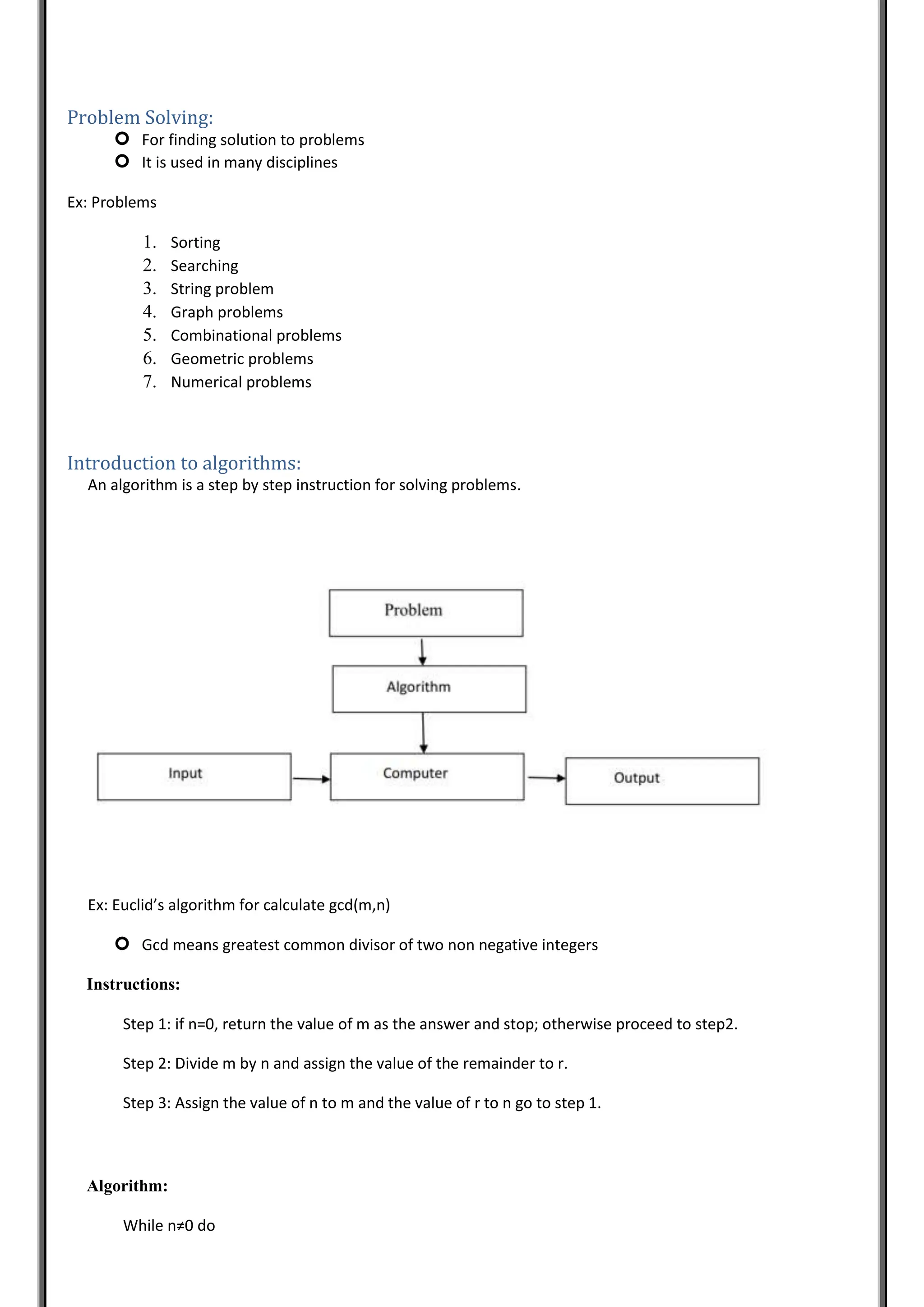
An algorithm is a step by step instruction for solving problems.
Ex: Euclid’s algorithm for calculate gcd(m,n)
 Gcd means greatest common divisor of two non negative integers
Instructions:
Step 1: if n=0, return the value of m as the answer and stop; otherwise proceed to step2.
Step 2: Divide m by n and assign the value of the remainder to r.
Step 3: Assign the value of n to m and the value of r to n go to step 1.
Algorithm:
While n≠0 do
r ← m mod n
m ← n
n ← r
return m
Characteristic of Algorithm:
1. Time efficiency – how fast the algorithm runs.
2. Space efficiency – how much extra memory used
3. Simplicity – simpler than the other algorithms
4. Generality –the algorithm solves and the range of inputs it accepts and used
more general terms.
Algorithm design tools:
1. Pseudo code
2. Flow chart
Pseudo Code:
• It is a mixture of a natural language and programming language Flow chart:
• Pictorial representation of an algorithm Analysis of an Algorithm:
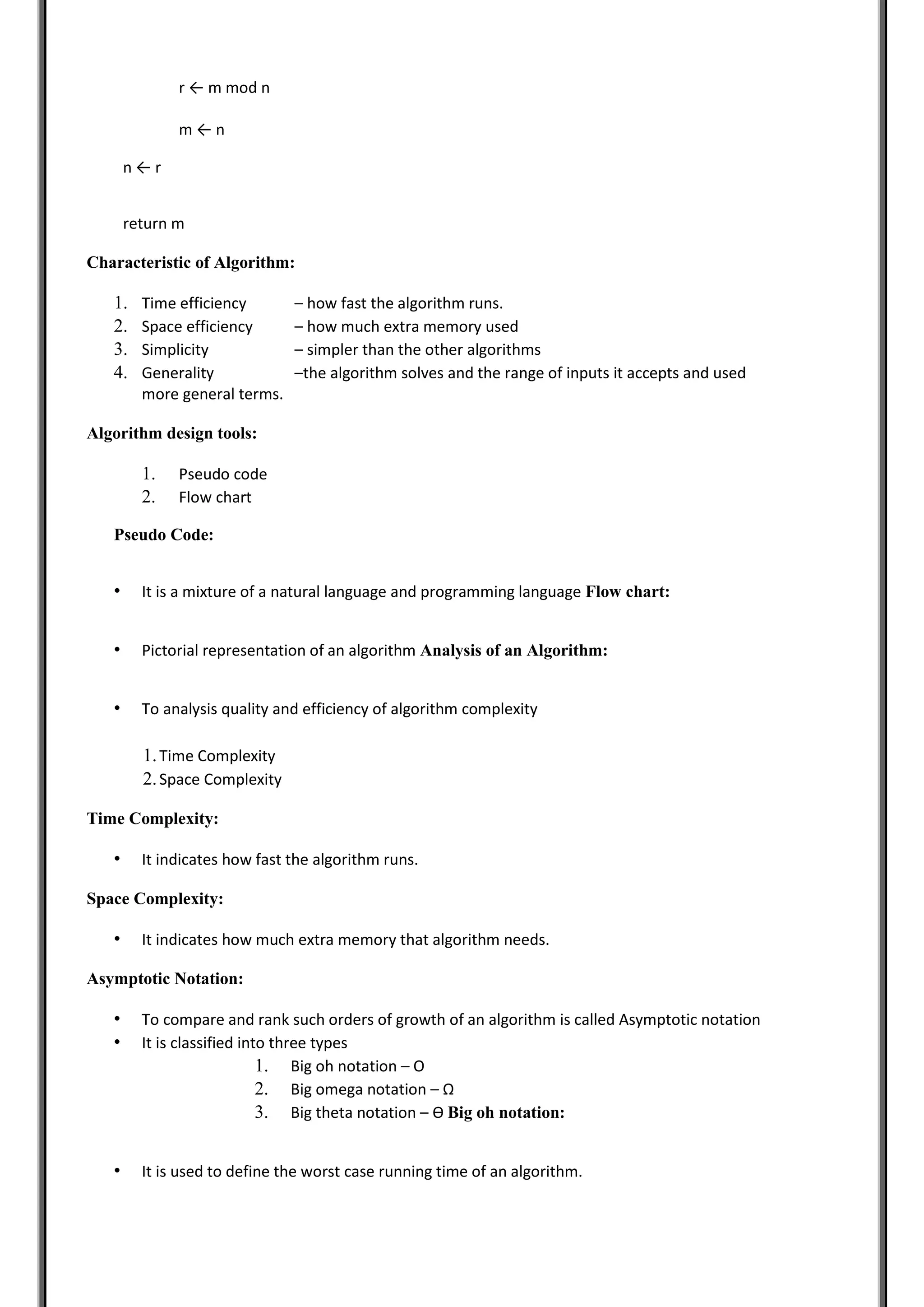
• To analysis quality and efficiency of algorithm complexity
1.Time Complexity
2.Space Complexity
Time Complexity:
• It indicates how fast the algorithm runs.
Space Complexity:
• It indicates how much extra memory that algorithm needs.
Asymptotic Notation:
• To compare and rank such orders of growth of an algorithm is called Asymptotic notation
• It is classified into three types
1. Big oh notation – O
2. Big omega notation – Ω
3. Big theta notation – Ɵ Big oh notation:
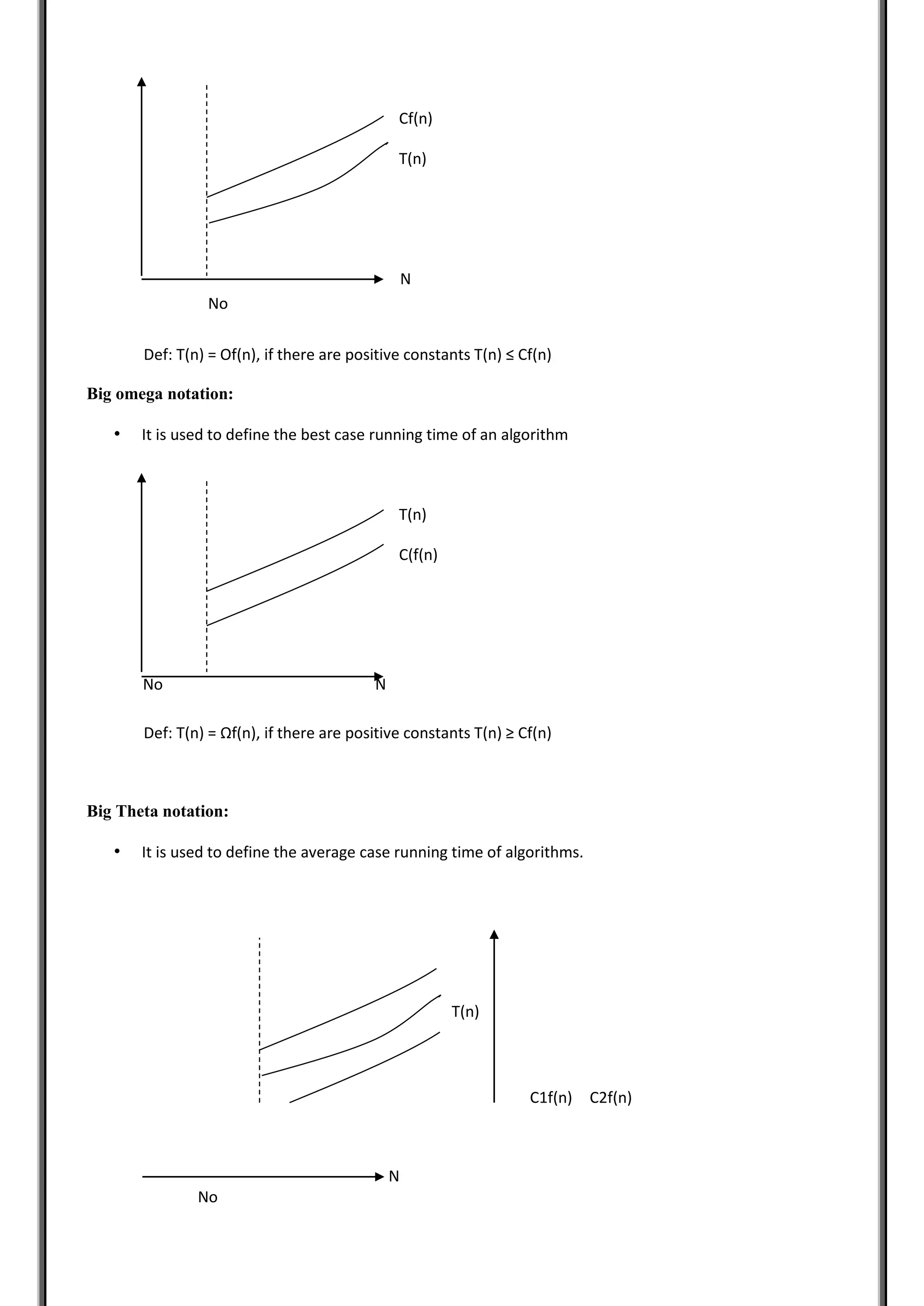
• It is used to define the worst case running time of an algorithm.
Def: T(n) = Of(n), if there are positive constants T(n) ≤ Cf(n)
Big omega notation:
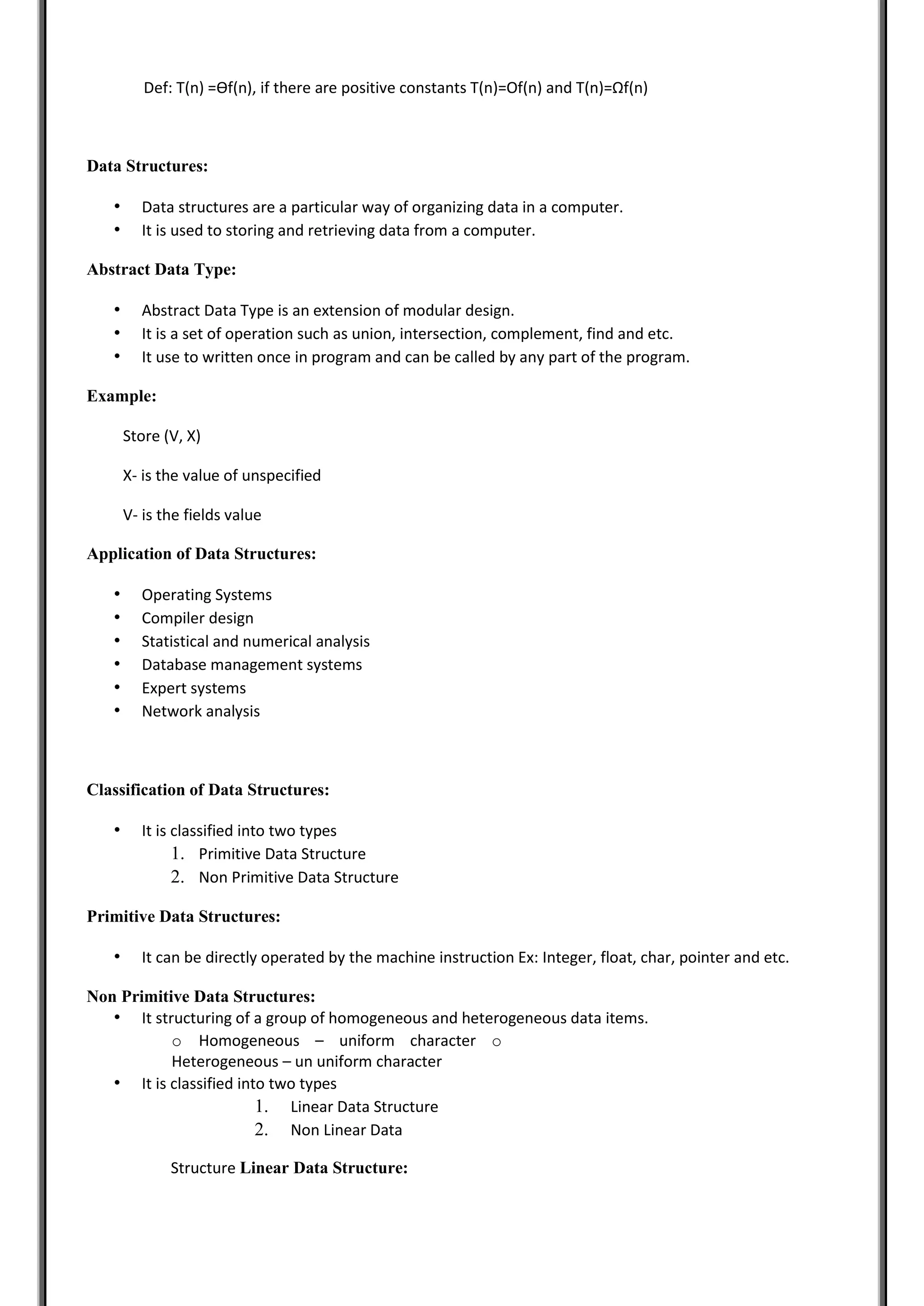
• It is used to define the best case running time of an algorithm
Def: T(n) = Ωf(n), if there are positive constants T(n) ≥ Cf(n)
Big Theta notation:
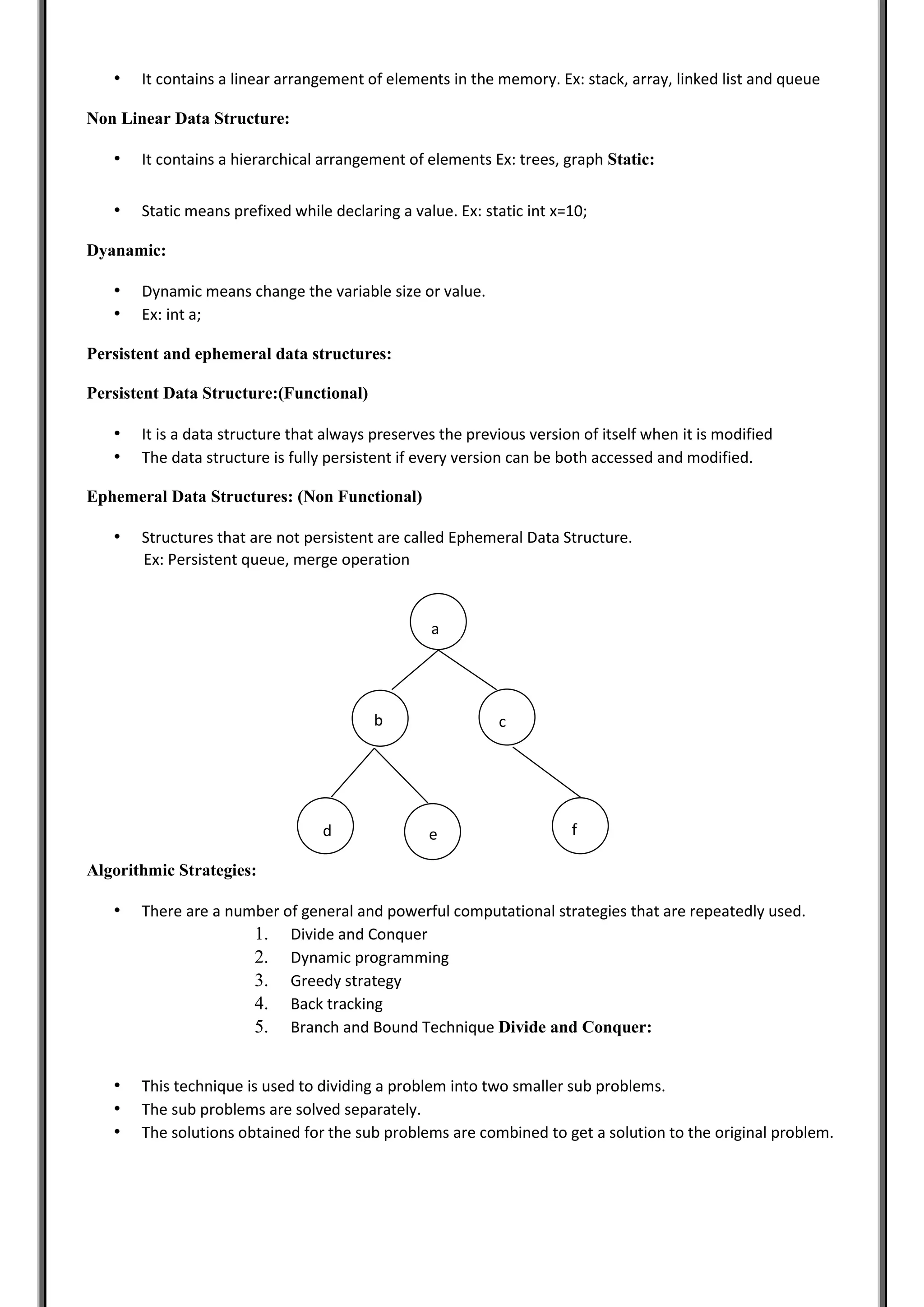
• It is used to define the average case running time of algorithms.
C1f(n) C2f(n)
N
No
Cf(n)
T(n)
N
No
T(n)
C(f(n)
No N
T(n)
Def: T(n) =Ɵf(n), if there are positive constants T(n)=Of(n) and T(n)=Ωf(n)
Data Structures:
• Data structures are a particular way of organizing data in a computer.
• It is used to storing and retrieving data from a computer.
Abstract Data Type:
• Abstract Data Type is an extension of modular design.
• It is a set of operation such as union, intersection, complement, find and etc.
• It use to written once in program and can be called by any part of the program.
Example:
Store (V, X)
X- is the value of unspecified
V- is the fields value
Application of Data Structures:
• Operating Systems
• Compiler design
• Statistical and numerical analysis
• Database management systems
• Expert systems
• Network analysis
Classification of Data Structures:
• It is classified into two types
1. Primitive Data Structure
2. Non Primitive Data Structure
Primitive Data Structures:
• It can be directly operated by the machine instruction Ex: Integer, float, char, pointer and etc.
Non Primitive Data Structures:
• It structuring of a group of homogeneous and heterogeneous data items.
o Homogeneous – uniform character o
Heterogeneous – un uniform character
• It is classified into two types
1. Linear Data Structure
2. Non Linear Data
Structure Linear Data Structure:
• It contains a linear arrangement of elements in the memory. Ex: stack, array, linked list and queue
Non Linear Data Structure:
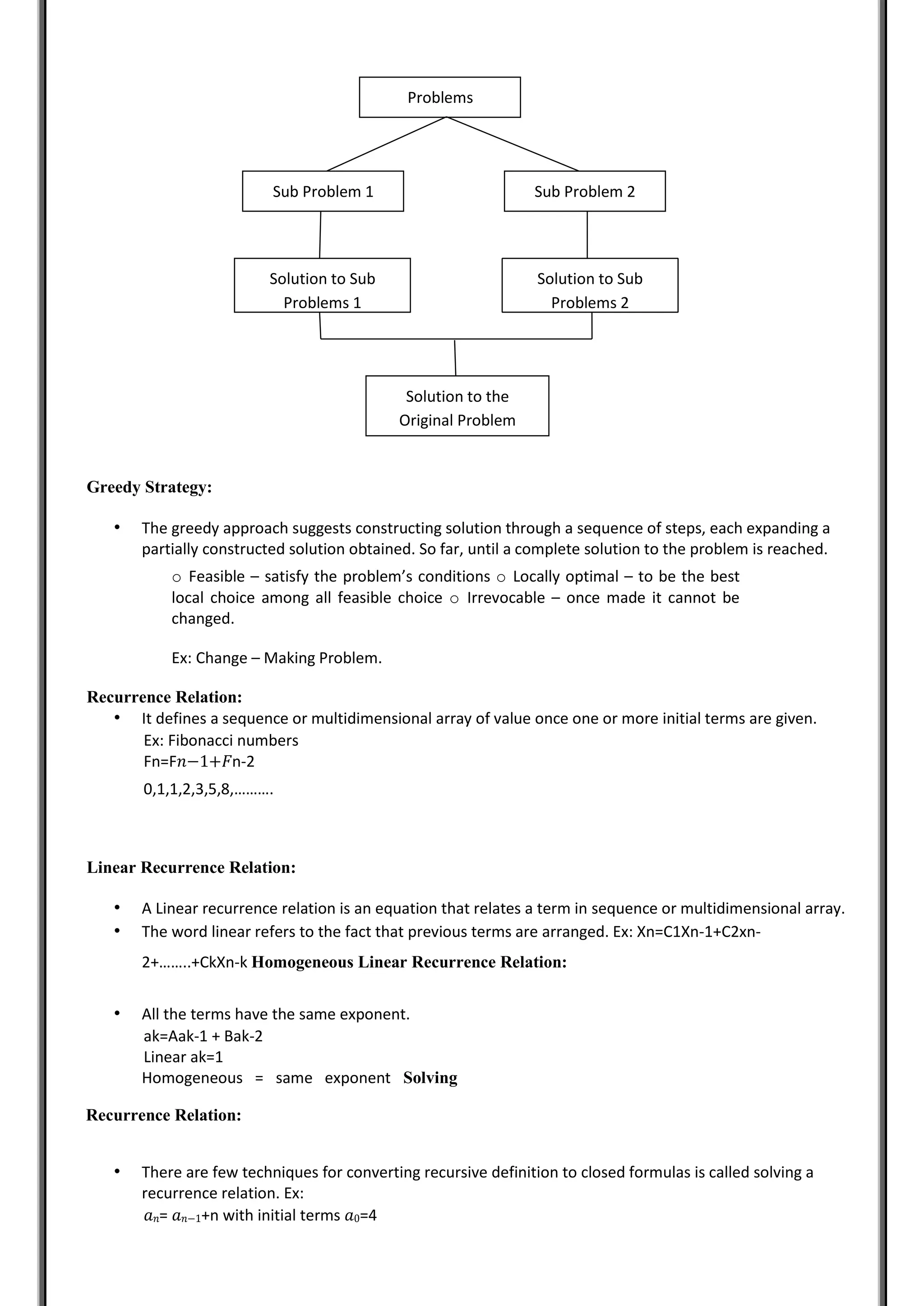
• It contains a hierarchical arrangement of elements Ex: trees, graph Static:
• Static means prefixed while declaring a value. Ex: static int x=10;
Dyanamic:
• Dynamic means change the variable size or value.
• Ex: int a;
Persistent and ephemeral data structures:
Persistent Data Structure:(Functional)
• It is a data structure that always preserves the previous version of itself when it is modified
• The data structure is fully persistent if every version can be both accessed and modified.
Ephemeral Data Structures: (Non Functional)
• Structures that are not persistent are called Ephemeral Data Structure.
Ex: Persistent queue, merge operation
Algorithmic Strategies:
• There are a number of general and powerful computational strategies that are repeatedly used.
1. Divide and Conquer
2. Dynamic programming
3. Greedy strategy
4. Back tracking
5. Branch and Bound Technique Divide and Conquer:
• This technique is used to dividing a problem into two smaller sub problems.
• The sub problems are solved separately.
• The solutions obtained for the sub problems are combined to get a solution to the original problem.
a
b c
d e f
Greedy Strategy:
• The greedy approach suggests constructing solution through a sequence of steps, each expanding a
partially constructed solution obtained. So far, until a complete solution to the problem is reached.
o Feasible – satisfy the problem’s conditions o Locally optimal – to be the best
local choice among all feasible choice o Irrevocable – once made it cannot be
changed.
Ex: Change – Making Problem.
Recurrence Relation:
• It defines a sequence or multidimensional array of value once one or more initial terms are given.
Ex: Fibonacci numbers
Fn=F𝑛−1+𝐹n-2
0,1,1,2,3,5,8,……….
Linear Recurrence Relation:
• A Linear recurrence relation is an equation that relates a term in sequence or multidimensional array.
• The word linear refers to the fact that previous terms are arranged. Ex: Xn=C1Xn-1+C2xn-
2+……..+CkXn-k Homogeneous Linear Recurrence Relation:
• All the terms have the same exponent.
ak=Aak-1 + Bak-2
Linear ak=1
Homogeneous = same exponent Solving
Recurrence Relation:
• There are few techniques for converting recursive definition to closed formulas is called solving a
recurrence relation. Ex:
𝑎𝑛= 𝑎𝑛−1+n with initial terms 𝑎0=4
Problems
Sub Problem 1 Sub Problem 2
Solution to Sub
Problems 1
Solution to the
Original Problem
Solution to Sub
Problems 2
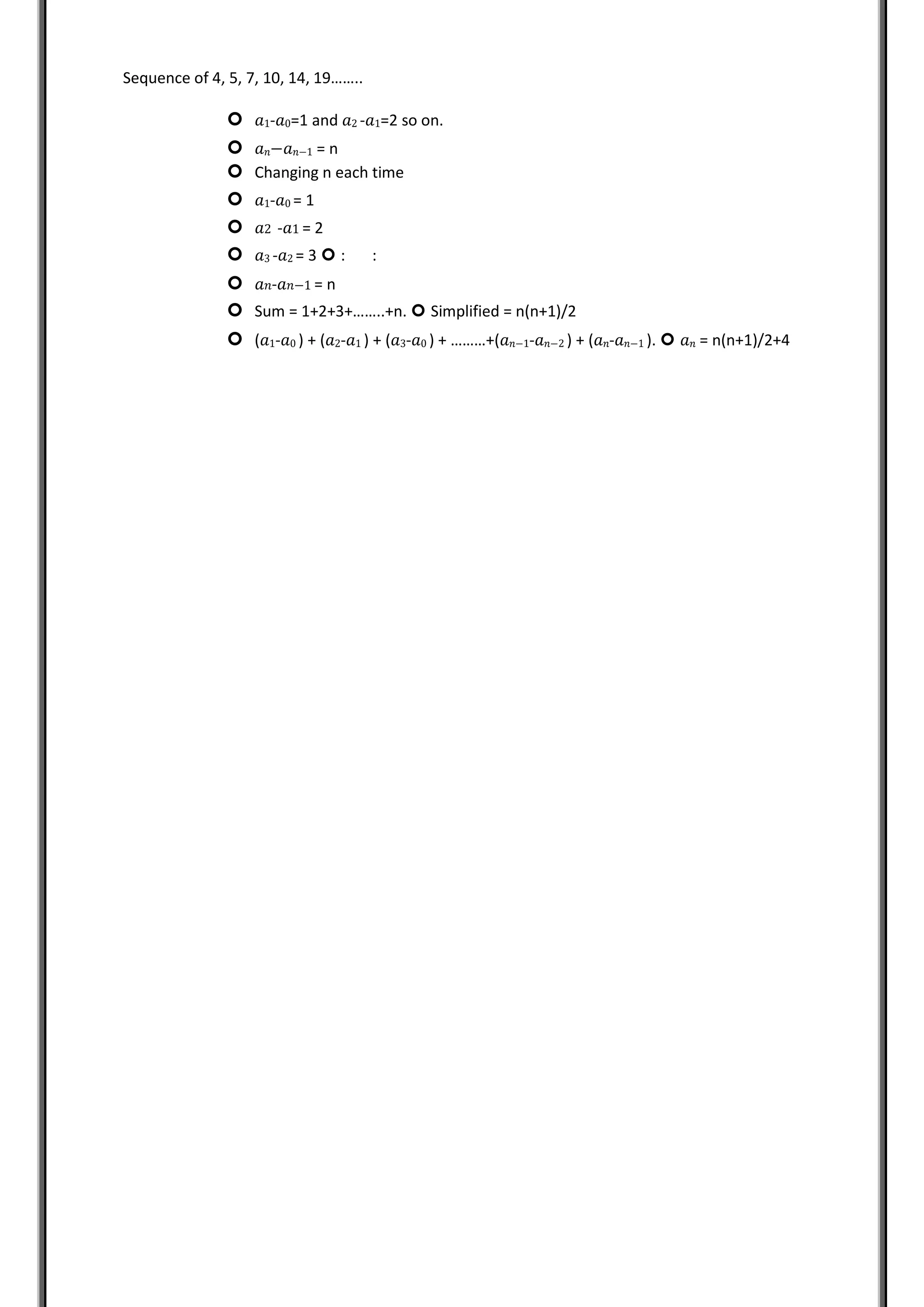
Sequence of 4, 5, 7, 10, 14, 19……..
 𝑎1-𝑎0=1 and 𝑎2 -𝑎1=2 so on.
 𝑎𝑛−𝑎𝑛−1 = n
 Changing n each time
 𝑎1-𝑎0 = 1
 𝑎2 -𝑎1 = 2
 𝑎3 -𝑎2 = 3  : :
 𝑎𝑛-𝑎𝑛−1 = n
 Sum = 1+2+3+……..+n.  Simplified = n(n+1)/2
 (𝑎1-𝑎0 ) + (𝑎2-𝑎1 ) + (𝑎3-𝑎0 ) + ………+(𝑎𝑛−1-𝑎𝑛−2 ) + (𝑎𝑛-𝑎𝑛−1 ).  𝑎𝑛 = n(n+1)/2+4

in computer data structures and algorithms

  • 1.
    DMI-ST. JOHN THEBAPTIST UNIVERSITY LILONGWE, MALAWI Module Code: 351CS34 Subject Name: DATA STRUCTURE AND ALGORITHM Unit I Detail Notes School of Computer Science Module Teacher: Fanny Chatola
  • 2.
    Syllabus Introduction to Algorithmand Data Structures: Algorithms- Problem Solving, Introduction to Algorithms, Characteristics of algorithms, Algorithm design tools: Pseudo code and flowchart, Analysis of Algorithms, Complexity of algorithms - Space complexity, Time complexity, Asymptotic notation - Big-O, Theta and Omega, standard measures of efficiency. Data Structures- Data structure, Abstract Data Types (ADT), Concept of linear and Non-linear, static and dynamic, persistent and ephemeral data structures, and relationship among data, data structure, and algorithm, From Problem to Program. Algorithmic Strategies- Introduction to algorithm design strategies - Divide and Conquer, and Greedy strategy. Recurrence relation - Recurrence Relation, Linear Recurrence Relations, With constant Coefficients, Homogeneous Solutions. Solving recurrence relations.
  • 3.
    TABLE OF CONTENTS Notable of contents entries found.
  • 4.
    Problem Solving:  Forfinding solution to problems  It is used in many disciplines Ex: Problems 1. Sorting 2. Searching 3. String problem 4. Graph problems 5. Combinational problems 6. Geometric problems 7. Numerical problems Introduction to algorithms: An algorithm is a step by step instruction for solving problems. Ex: Euclid’s algorithm for calculate gcd(m,n)  Gcd means greatest common divisor of two non negative integers Instructions: Step 1: if n=0, return the value of m as the answer and stop; otherwise proceed to step2. Step 2: Divide m by n and assign the value of the remainder to r. Step 3: Assign the value of n to m and the value of r to n go to step 1. Algorithm: While n≠0 do
  • 5.
    r ← mmod n m ← n n ← r return m Characteristic of Algorithm: 1. Time efficiency – how fast the algorithm runs. 2. Space efficiency – how much extra memory used 3. Simplicity – simpler than the other algorithms 4. Generality –the algorithm solves and the range of inputs it accepts and used more general terms. Algorithm design tools: 1. Pseudo code 2. Flow chart Pseudo Code: • It is a mixture of a natural language and programming language Flow chart: • Pictorial representation of an algorithm Analysis of an Algorithm: • To analysis quality and efficiency of algorithm complexity 1.Time Complexity 2.Space Complexity Time Complexity: • It indicates how fast the algorithm runs. Space Complexity: • It indicates how much extra memory that algorithm needs. Asymptotic Notation: • To compare and rank such orders of growth of an algorithm is called Asymptotic notation • It is classified into three types 1. Big oh notation – O 2. Big omega notation – Ω 3. Big theta notation – Ɵ Big oh notation: • It is used to define the worst case running time of an algorithm.
  • 6.
    Def: T(n) =Of(n), if there are positive constants T(n) ≤ Cf(n) Big omega notation: • It is used to define the best case running time of an algorithm Def: T(n) = Ωf(n), if there are positive constants T(n) ≥ Cf(n) Big Theta notation: • It is used to define the average case running time of algorithms. C1f(n) C2f(n) N No Cf(n) T(n) N No T(n) C(f(n) No N T(n)
  • 7.
    Def: T(n) =Ɵf(n),if there are positive constants T(n)=Of(n) and T(n)=Ωf(n) Data Structures: • Data structures are a particular way of organizing data in a computer. • It is used to storing and retrieving data from a computer. Abstract Data Type: • Abstract Data Type is an extension of modular design. • It is a set of operation such as union, intersection, complement, find and etc. • It use to written once in program and can be called by any part of the program. Example: Store (V, X) X- is the value of unspecified V- is the fields value Application of Data Structures: • Operating Systems • Compiler design • Statistical and numerical analysis • Database management systems • Expert systems • Network analysis Classification of Data Structures: • It is classified into two types 1. Primitive Data Structure 2. Non Primitive Data Structure Primitive Data Structures: • It can be directly operated by the machine instruction Ex: Integer, float, char, pointer and etc. Non Primitive Data Structures: • It structuring of a group of homogeneous and heterogeneous data items. o Homogeneous – uniform character o Heterogeneous – un uniform character • It is classified into two types 1. Linear Data Structure 2. Non Linear Data Structure Linear Data Structure:
  • 8.
    • It containsa linear arrangement of elements in the memory. Ex: stack, array, linked list and queue Non Linear Data Structure: • It contains a hierarchical arrangement of elements Ex: trees, graph Static: • Static means prefixed while declaring a value. Ex: static int x=10; Dyanamic: • Dynamic means change the variable size or value. • Ex: int a; Persistent and ephemeral data structures: Persistent Data Structure:(Functional) • It is a data structure that always preserves the previous version of itself when it is modified • The data structure is fully persistent if every version can be both accessed and modified. Ephemeral Data Structures: (Non Functional) • Structures that are not persistent are called Ephemeral Data Structure. Ex: Persistent queue, merge operation Algorithmic Strategies: • There are a number of general and powerful computational strategies that are repeatedly used. 1. Divide and Conquer 2. Dynamic programming 3. Greedy strategy 4. Back tracking 5. Branch and Bound Technique Divide and Conquer: • This technique is used to dividing a problem into two smaller sub problems. • The sub problems are solved separately. • The solutions obtained for the sub problems are combined to get a solution to the original problem. a b c d e f
  • 9.
    Greedy Strategy: • Thegreedy approach suggests constructing solution through a sequence of steps, each expanding a partially constructed solution obtained. So far, until a complete solution to the problem is reached. o Feasible – satisfy the problem’s conditions o Locally optimal – to be the best local choice among all feasible choice o Irrevocable – once made it cannot be changed. Ex: Change – Making Problem. Recurrence Relation: • It defines a sequence or multidimensional array of value once one or more initial terms are given. Ex: Fibonacci numbers Fn=F𝑛−1+𝐹n-2 0,1,1,2,3,5,8,………. Linear Recurrence Relation: • A Linear recurrence relation is an equation that relates a term in sequence or multidimensional array. • The word linear refers to the fact that previous terms are arranged. Ex: Xn=C1Xn-1+C2xn- 2+……..+CkXn-k Homogeneous Linear Recurrence Relation: • All the terms have the same exponent. ak=Aak-1 + Bak-2 Linear ak=1 Homogeneous = same exponent Solving Recurrence Relation: • There are few techniques for converting recursive definition to closed formulas is called solving a recurrence relation. Ex: 𝑎𝑛= 𝑎𝑛−1+n with initial terms 𝑎0=4 Problems Sub Problem 1 Sub Problem 2 Solution to Sub Problems 1 Solution to the Original Problem Solution to Sub Problems 2
  • 10.
    Sequence of 4,5, 7, 10, 14, 19……..  𝑎1-𝑎0=1 and 𝑎2 -𝑎1=2 so on.  𝑎𝑛−𝑎𝑛−1 = n  Changing n each time  𝑎1-𝑎0 = 1  𝑎2 -𝑎1 = 2  𝑎3 -𝑎2 = 3  : :  𝑎𝑛-𝑎𝑛−1 = n  Sum = 1+2+3+……..+n.  Simplified = n(n+1)/2  (𝑎1-𝑎0 ) + (𝑎2-𝑎1 ) + (𝑎3-𝑎0 ) + ………+(𝑎𝑛−1-𝑎𝑛−2 ) + (𝑎𝑛-𝑎𝑛−1 ).  𝑎𝑛 = n(n+1)/2+4