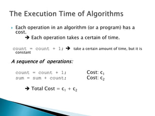
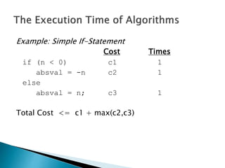
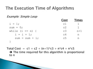
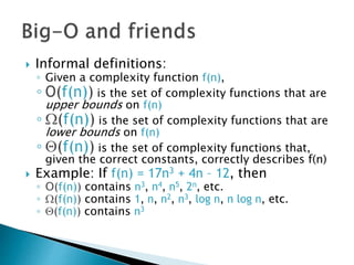
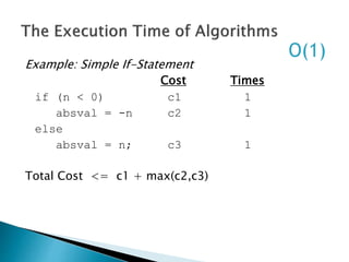
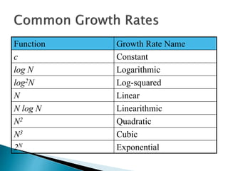
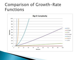
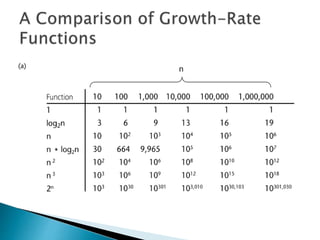
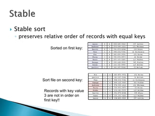
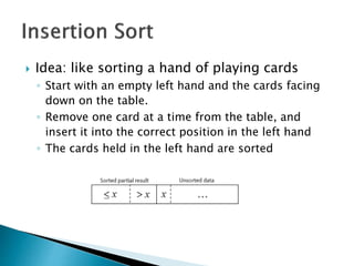
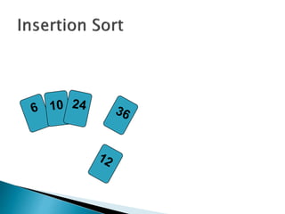
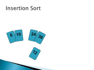
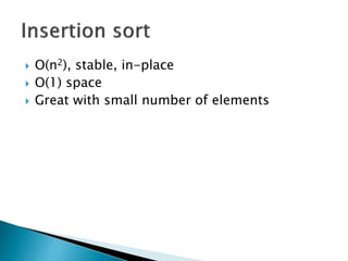
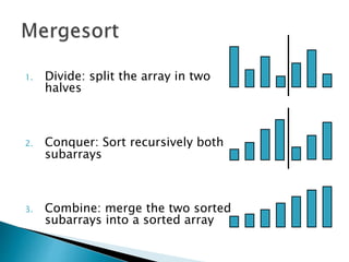
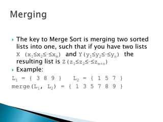
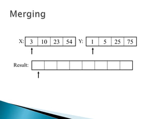
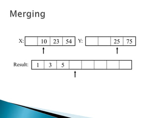
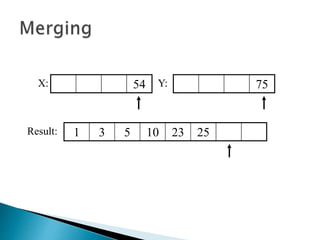
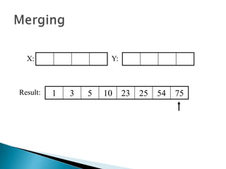
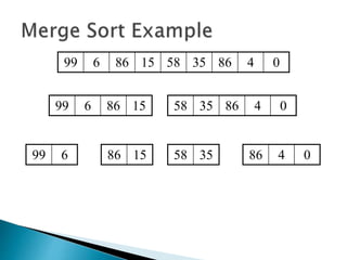
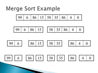
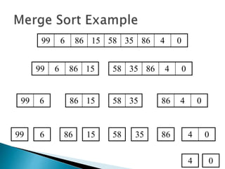
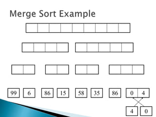
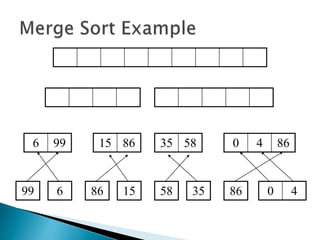
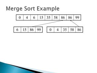
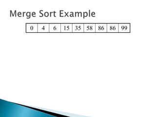
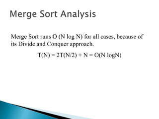
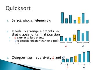
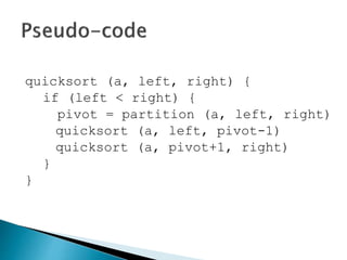
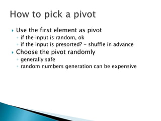
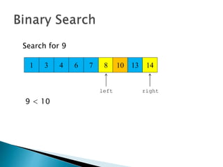
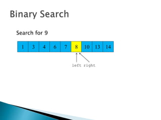
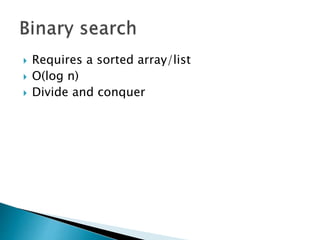
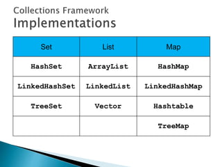
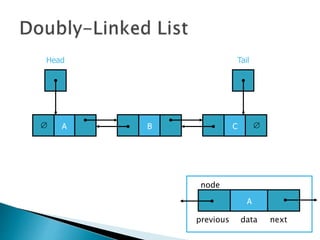
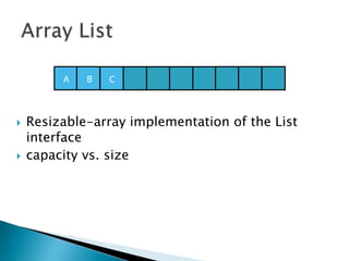
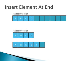
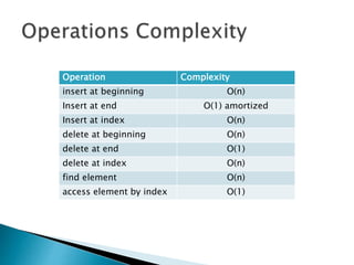
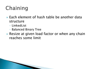
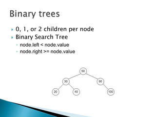
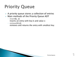
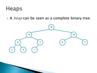
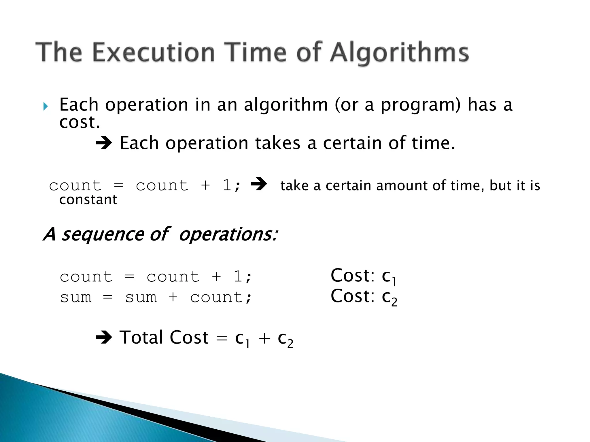
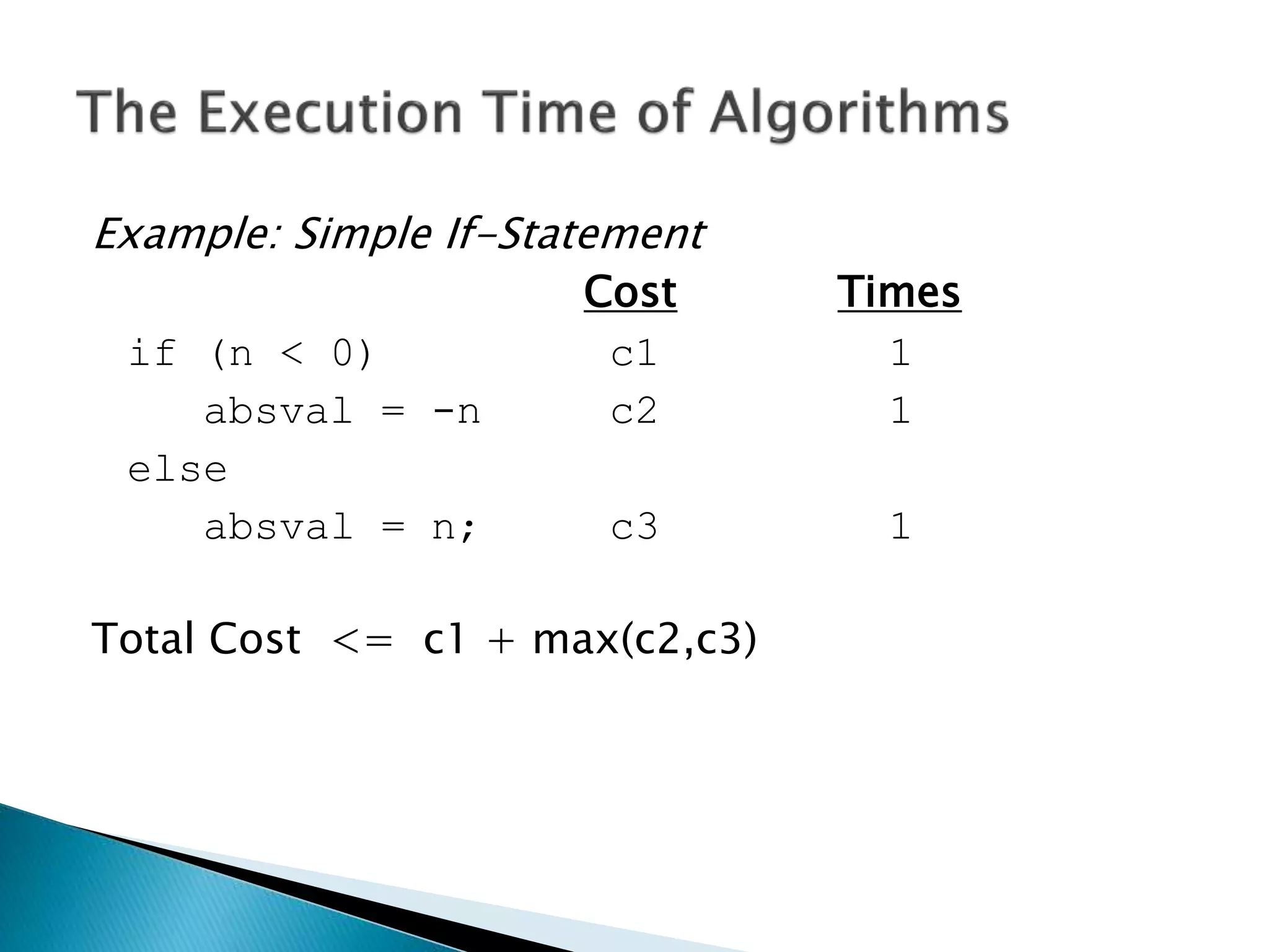
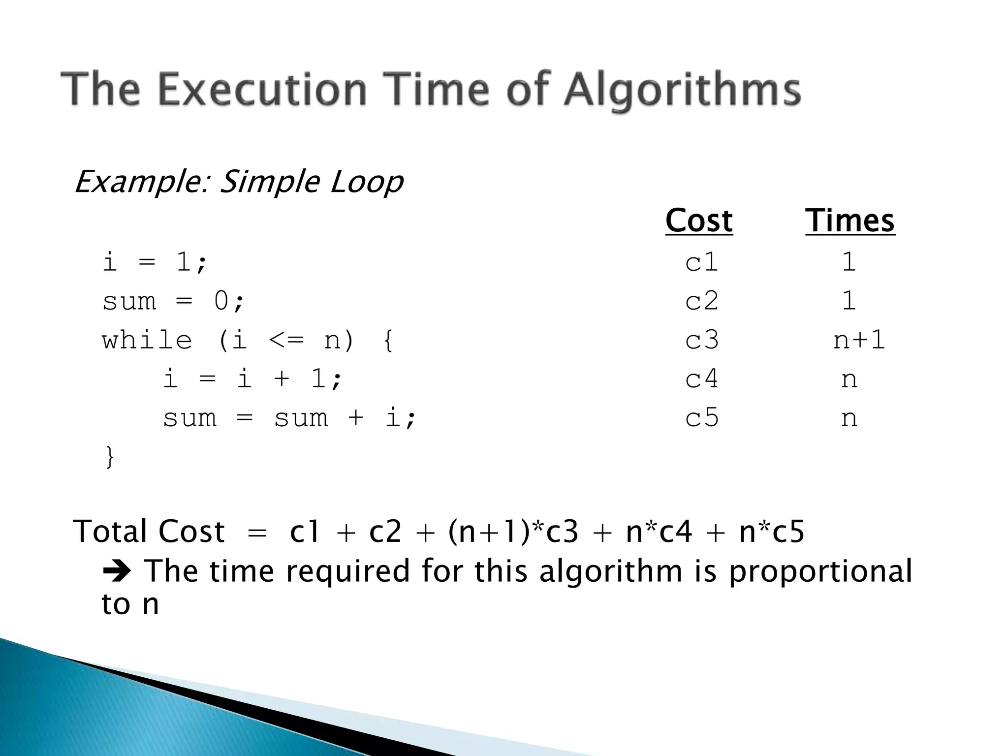
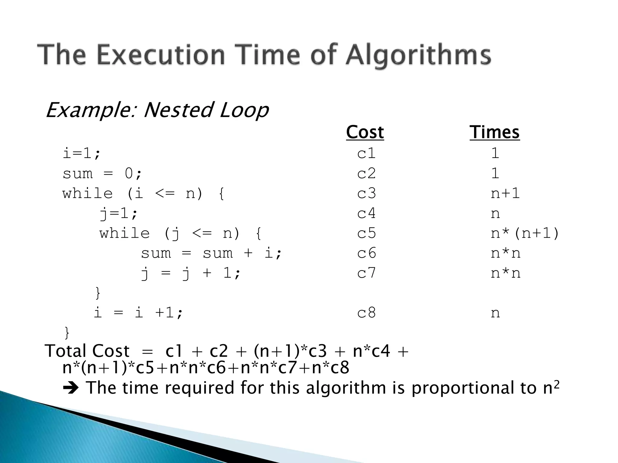
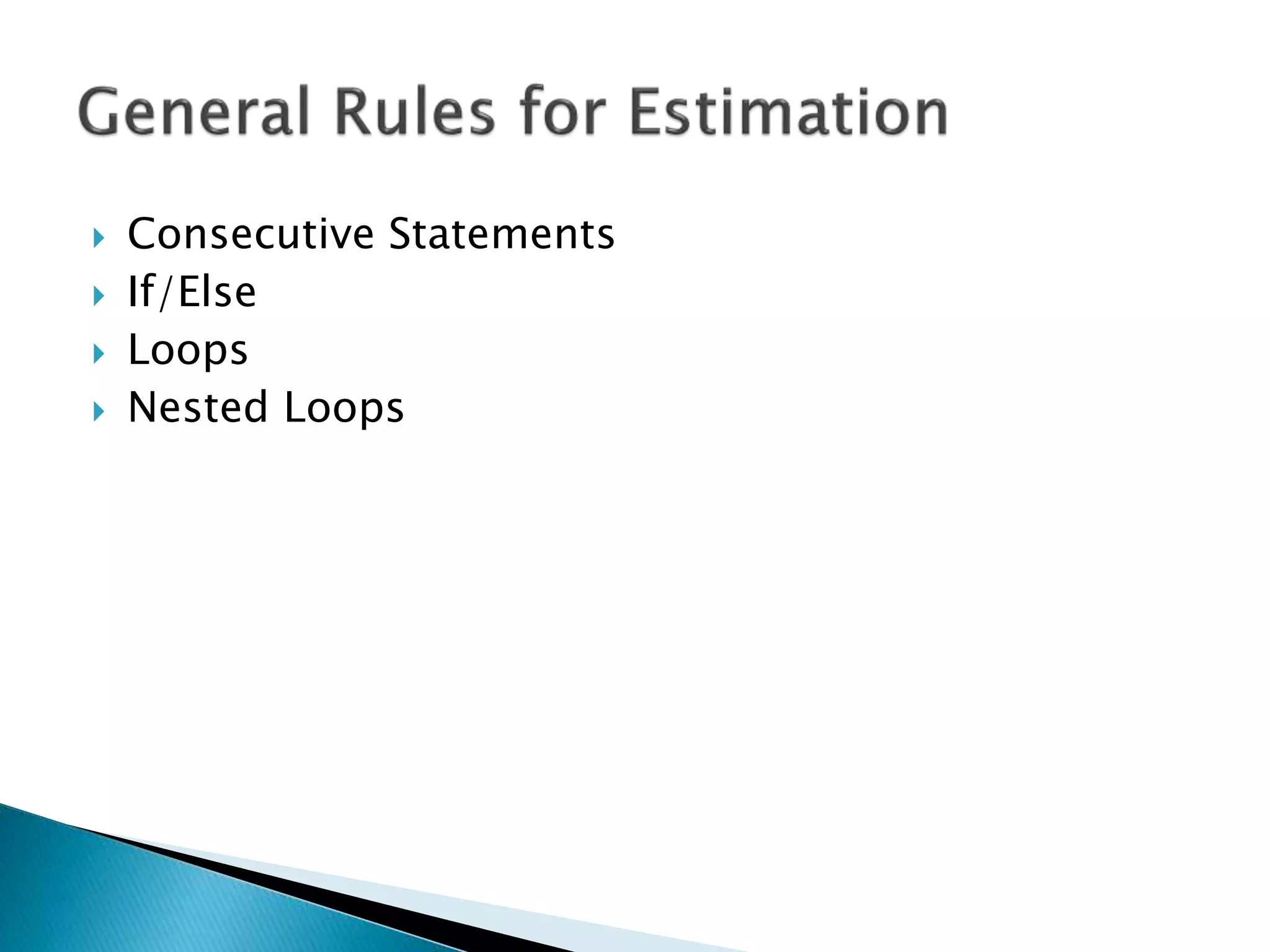
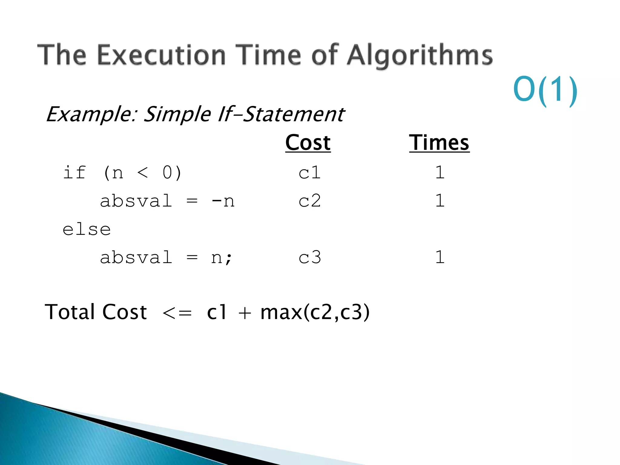
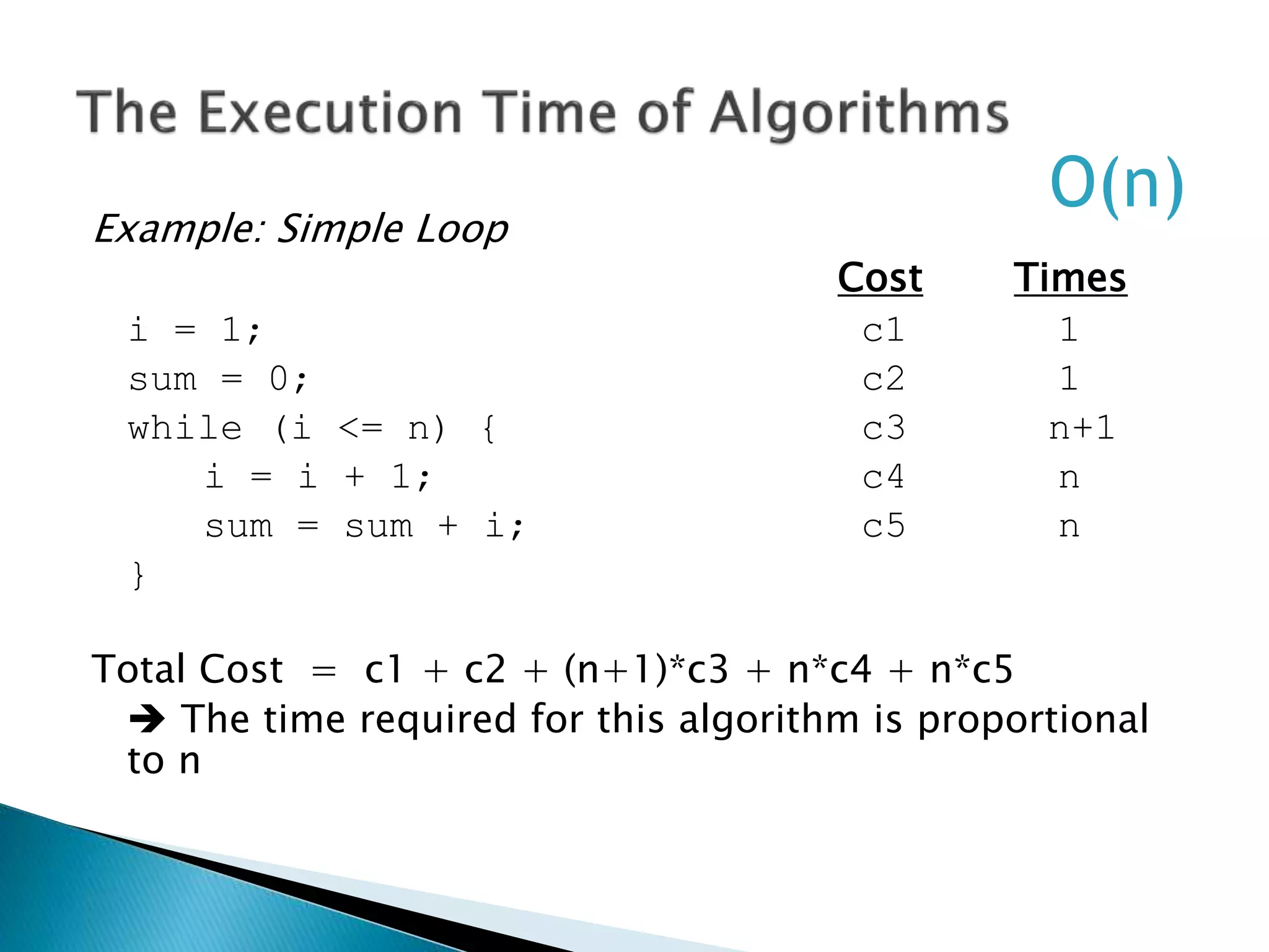
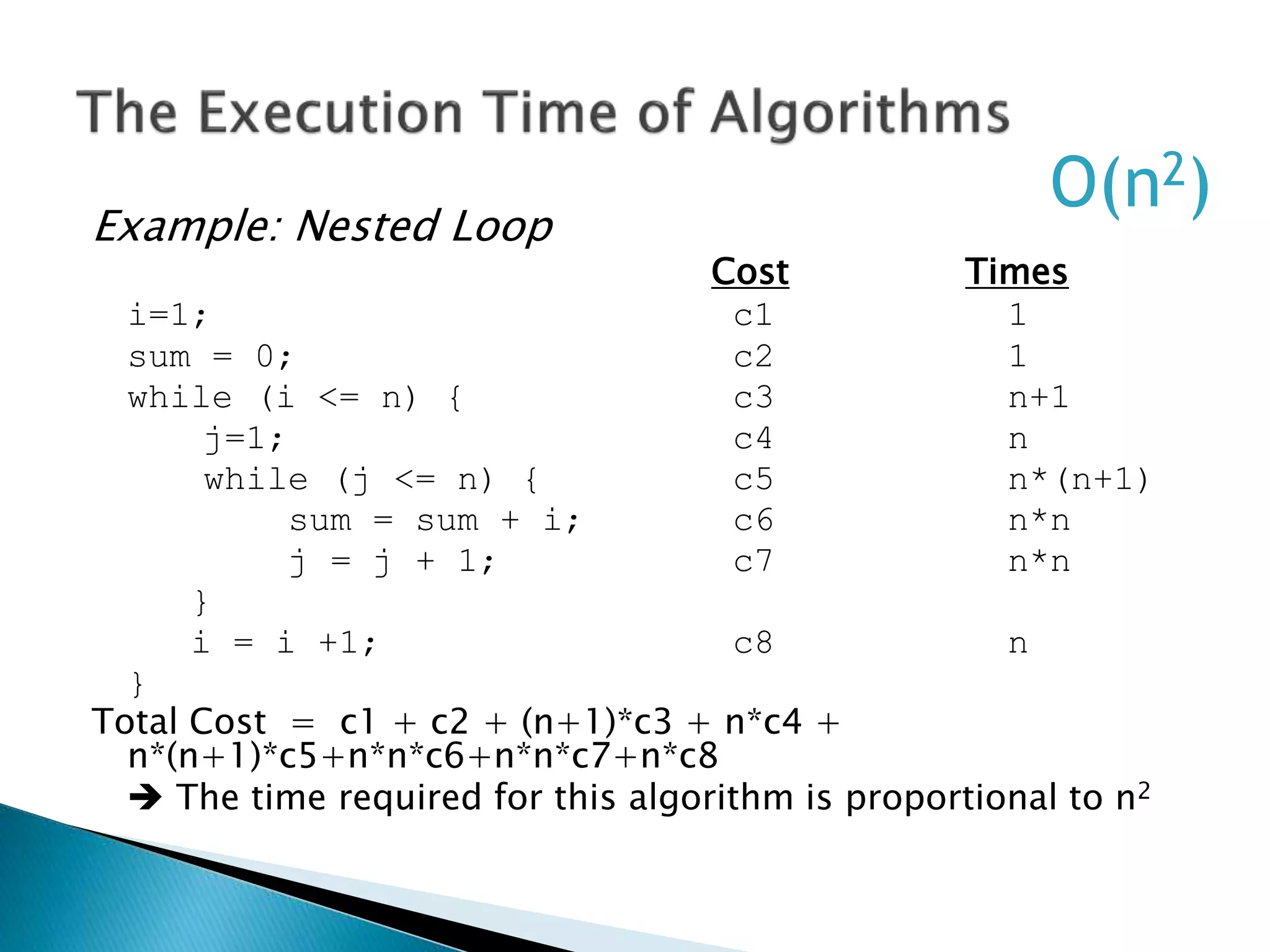
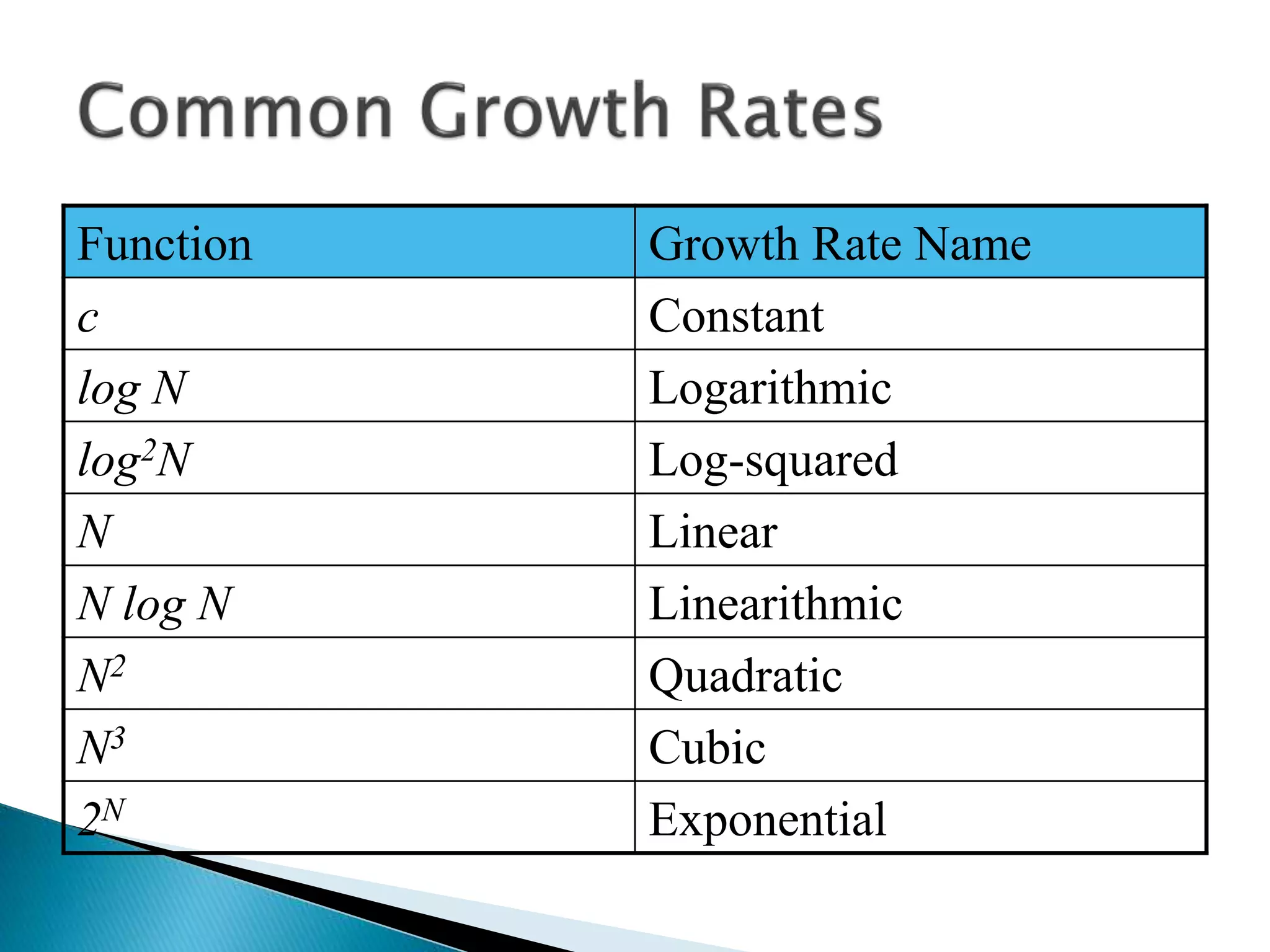
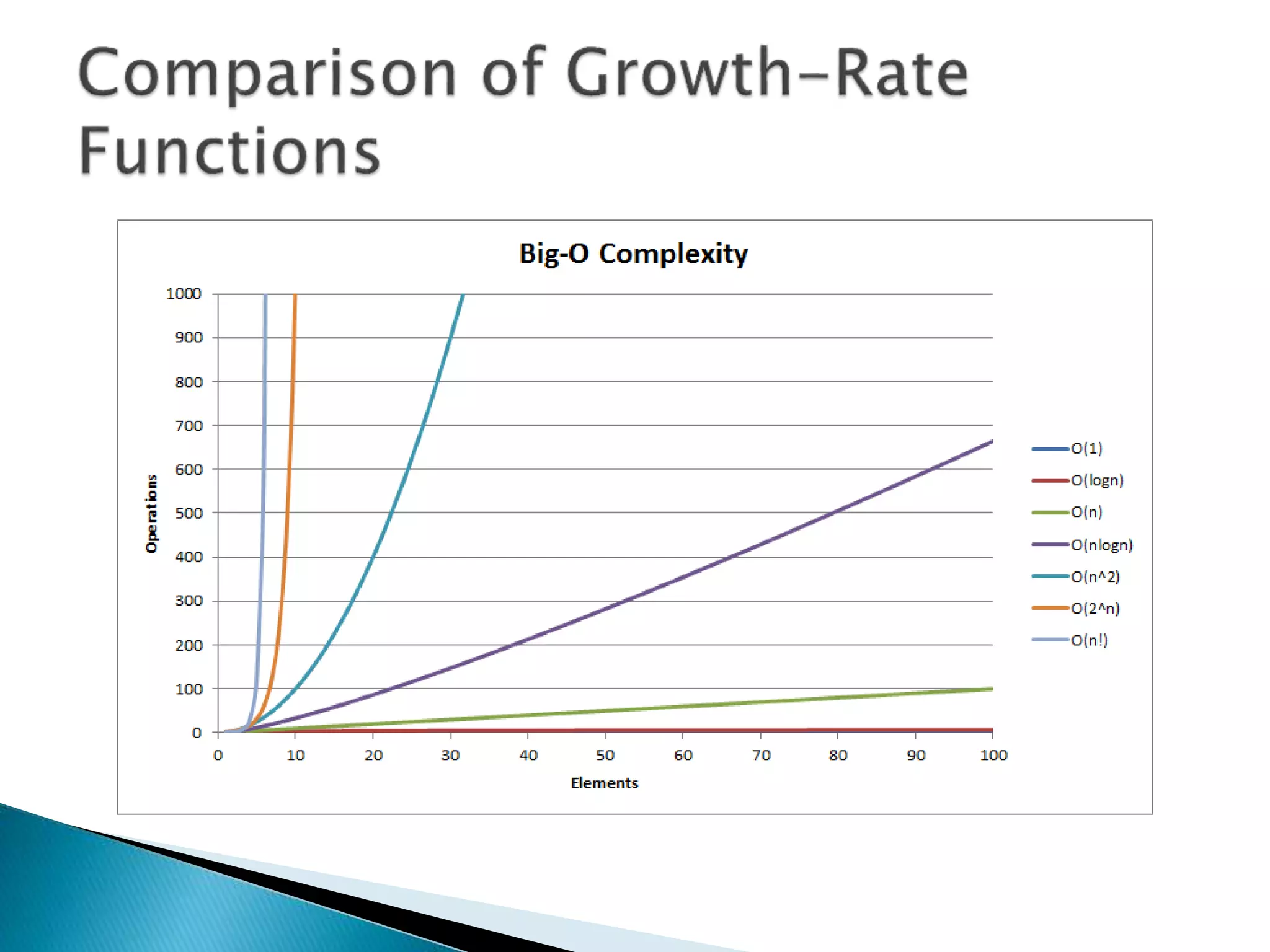
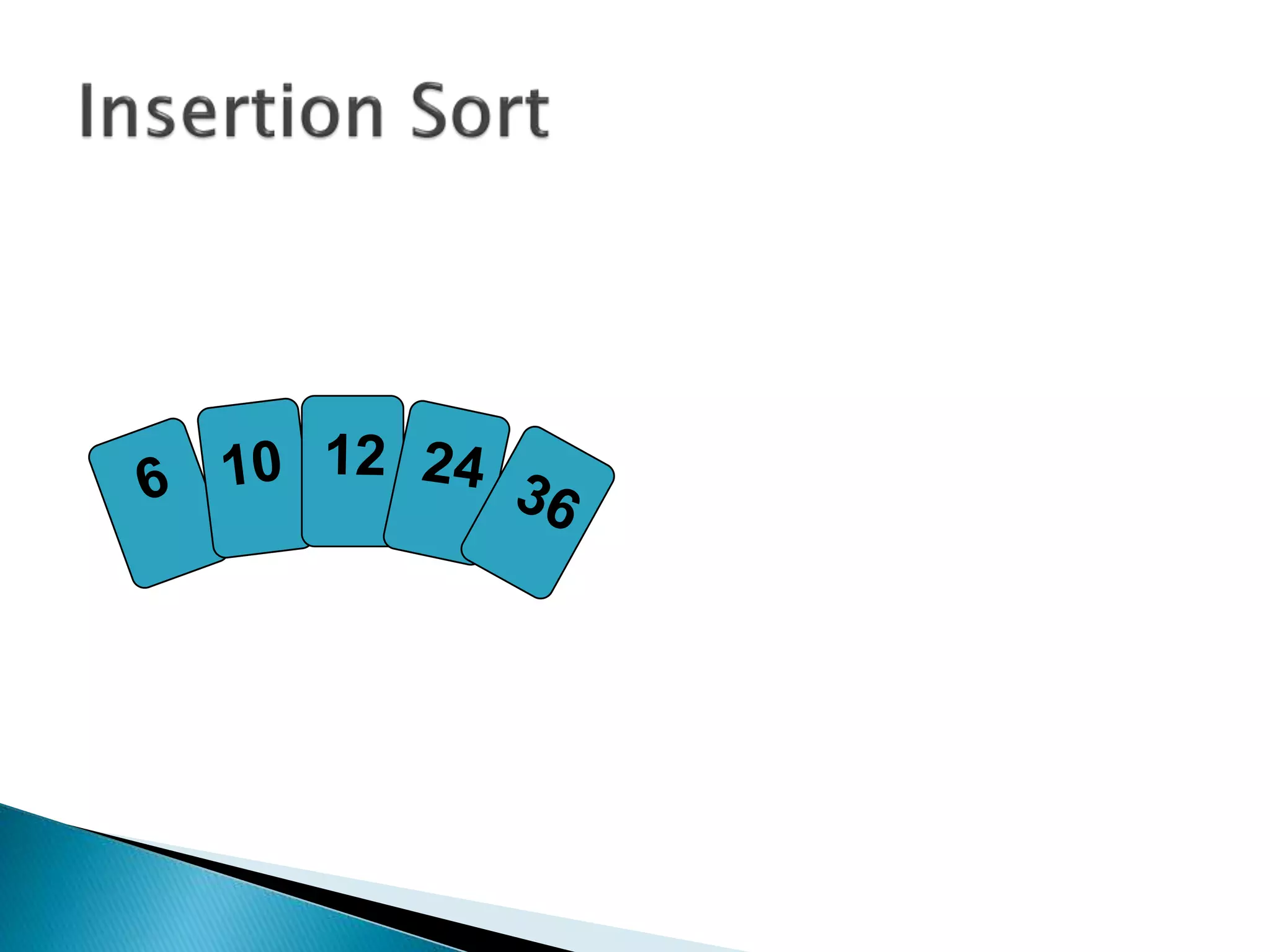
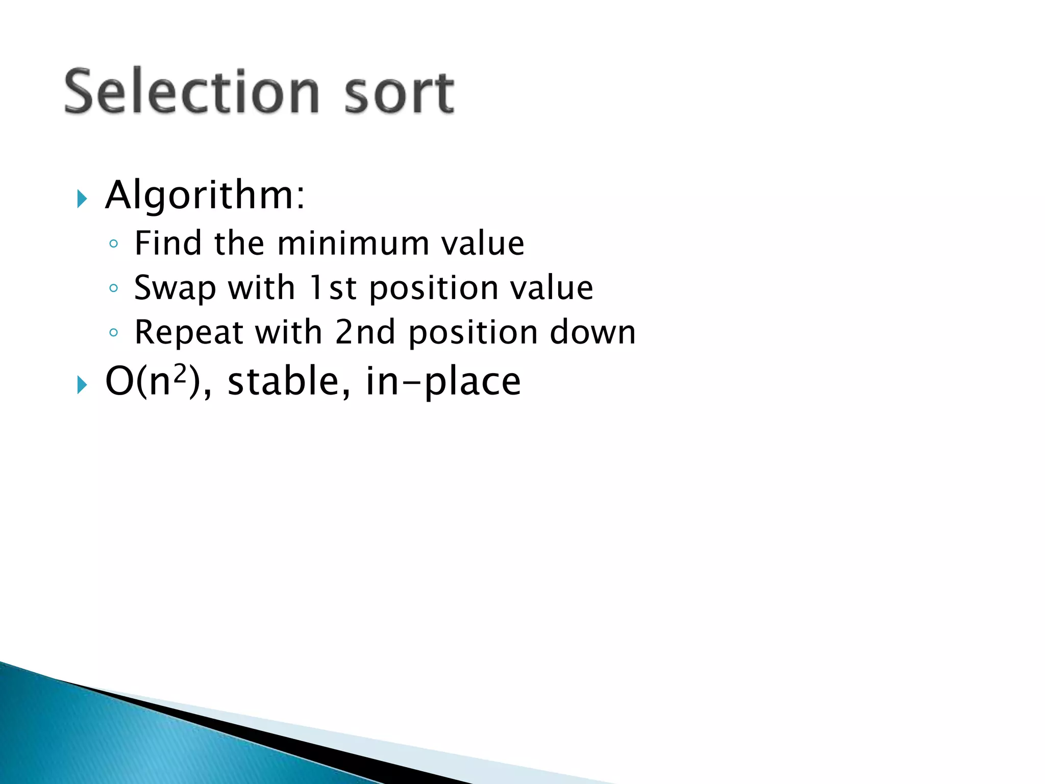
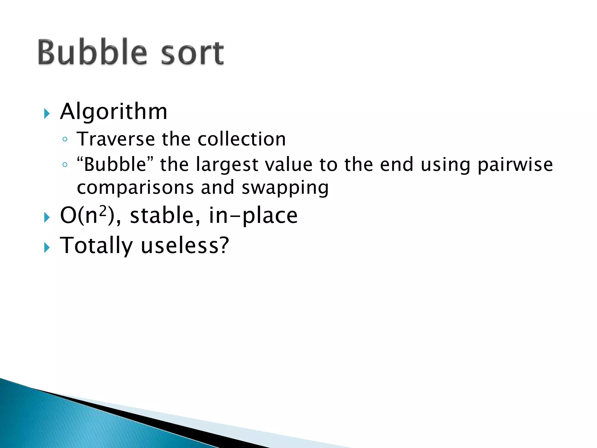
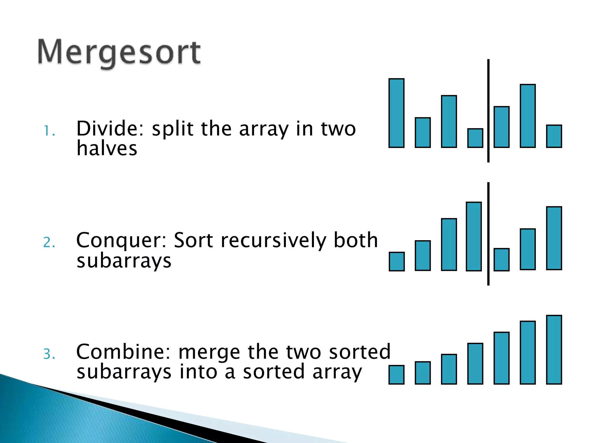
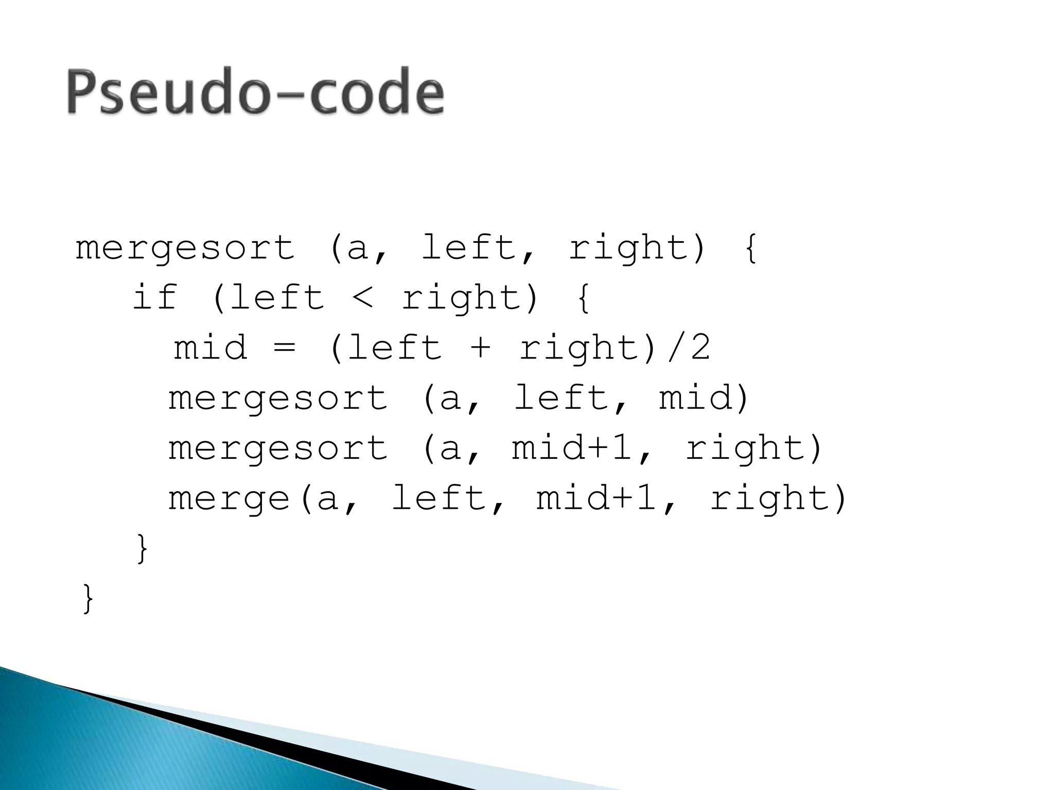
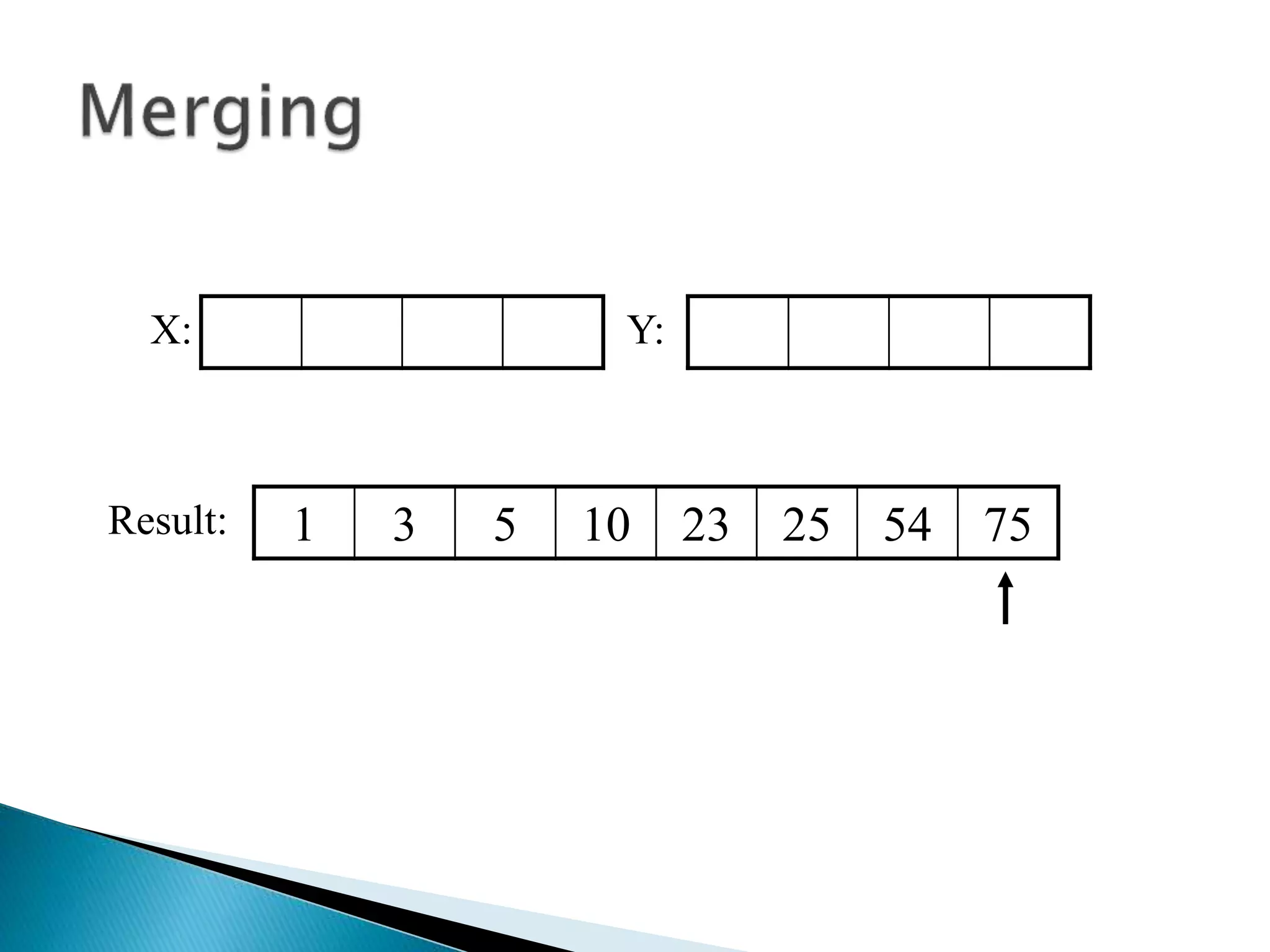
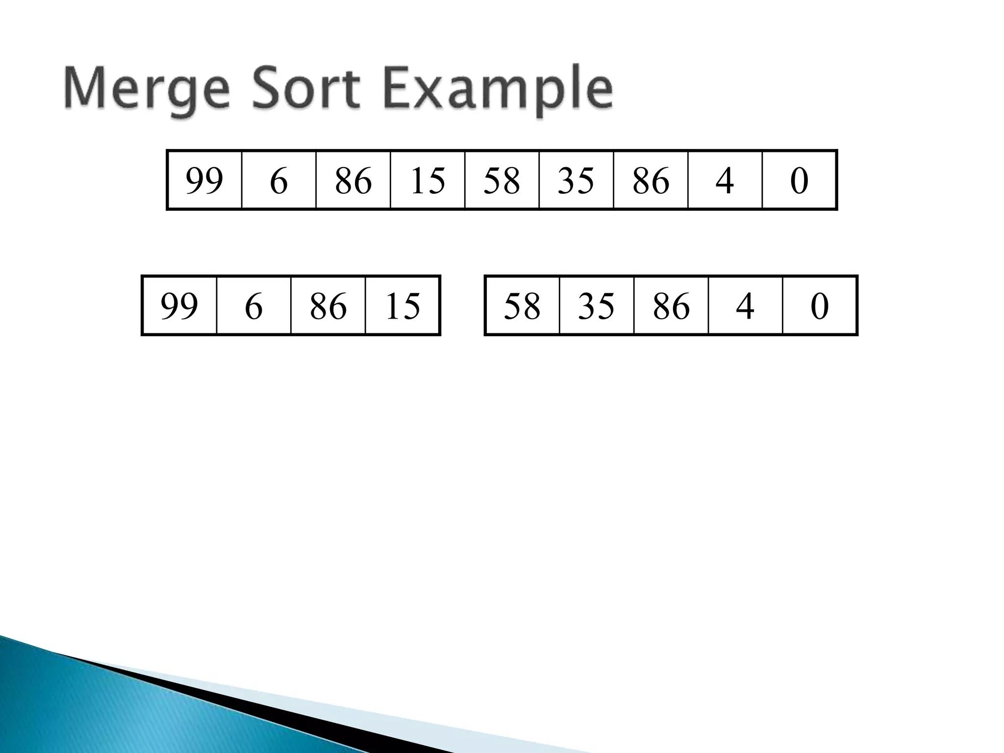
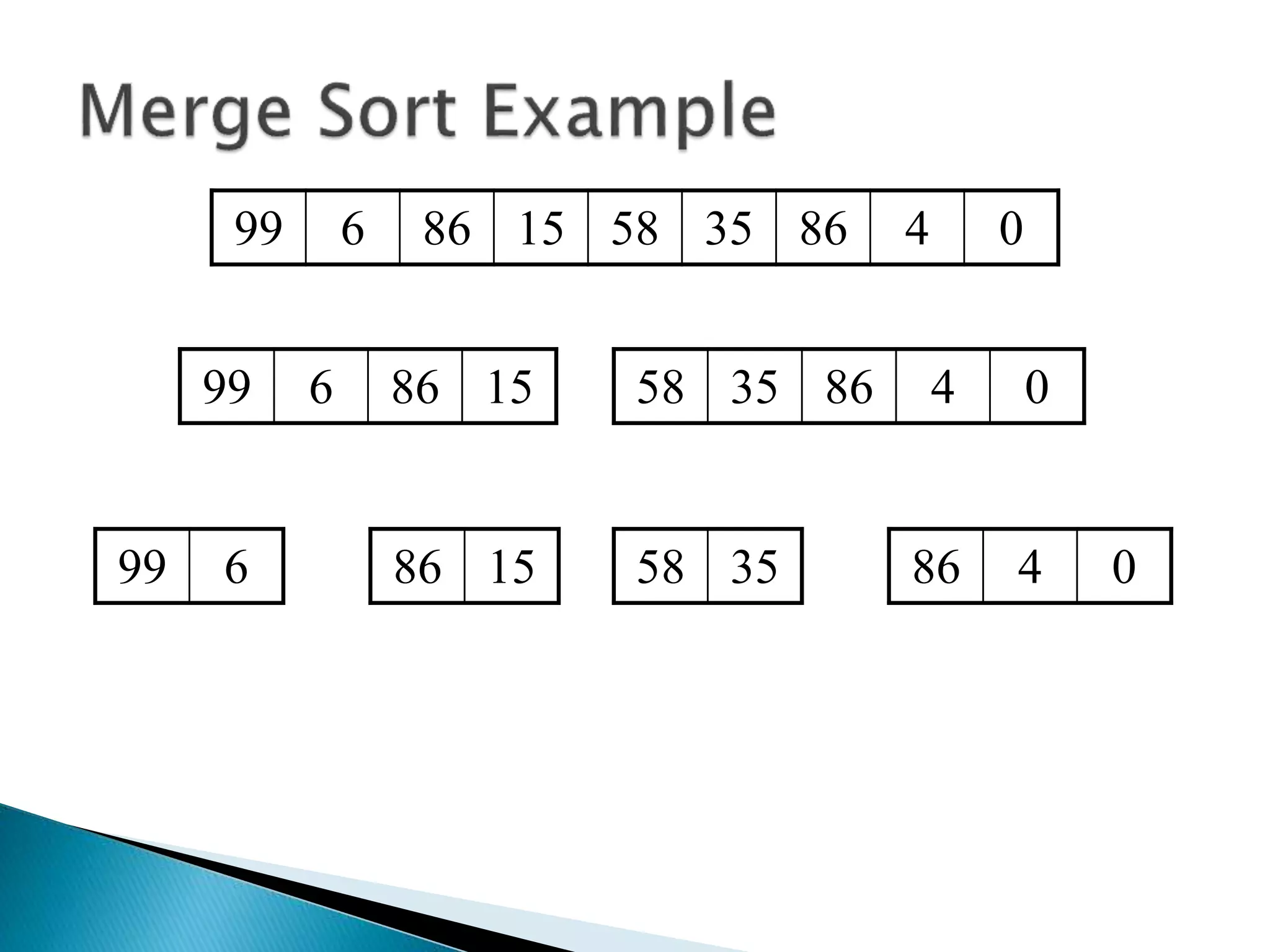
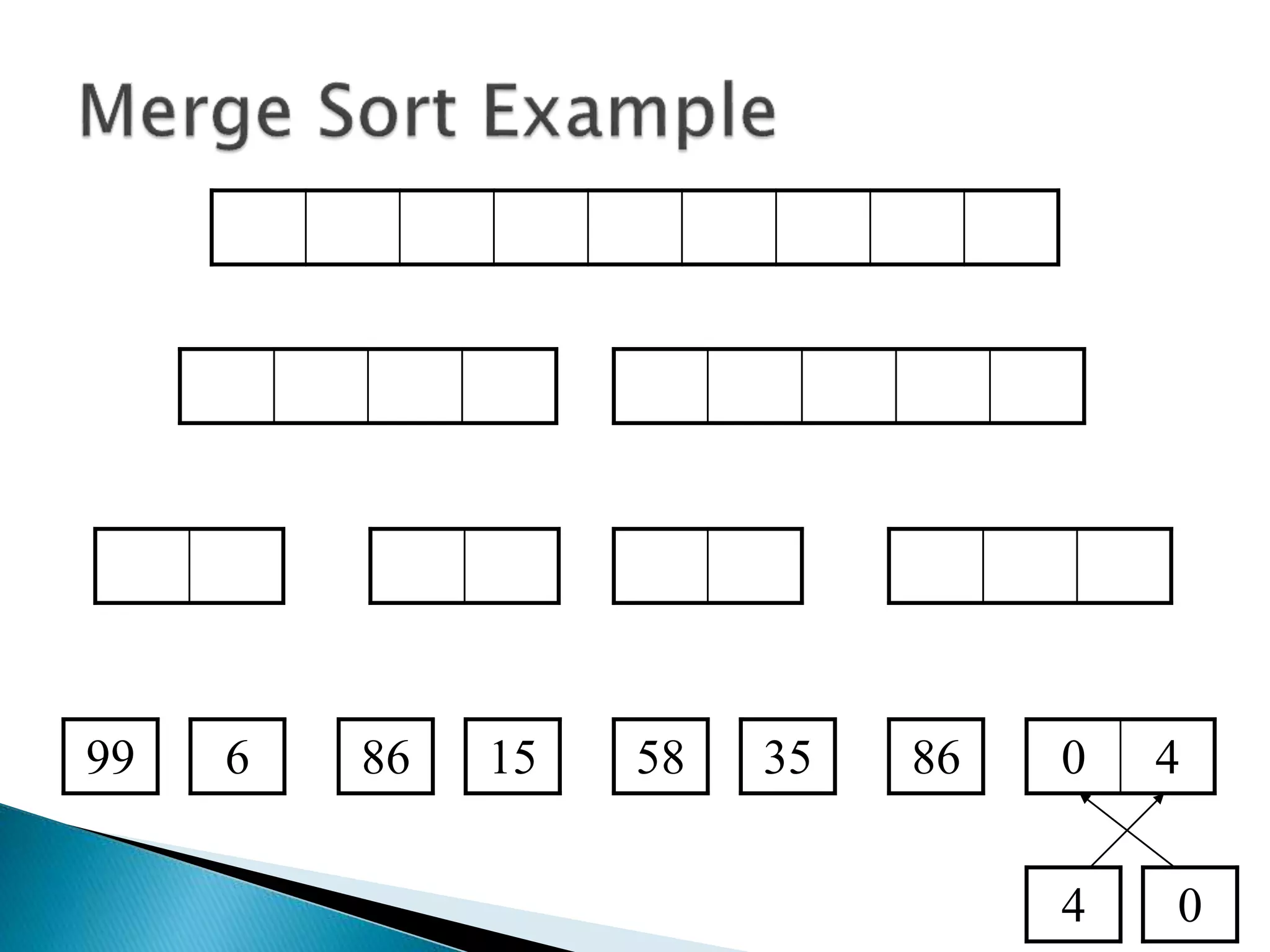
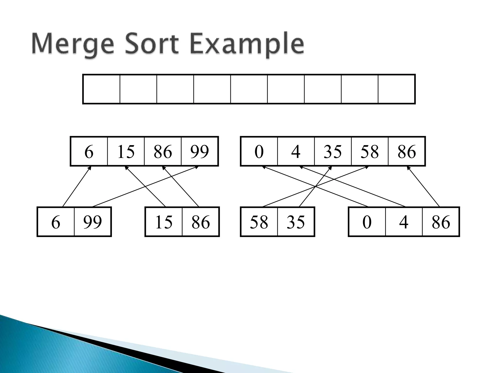
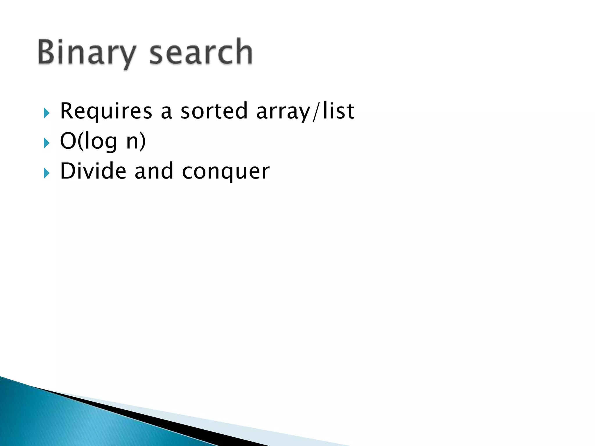
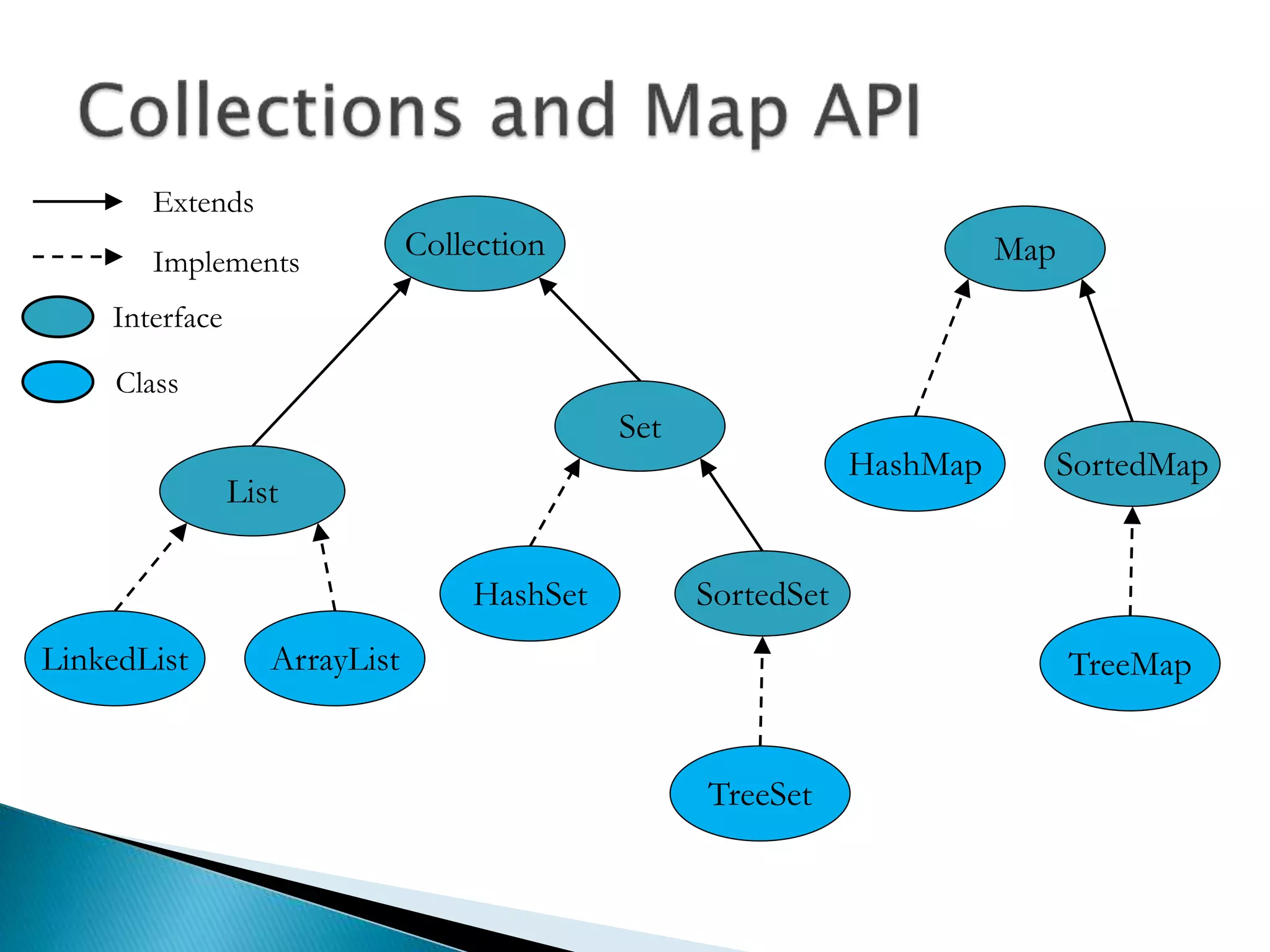
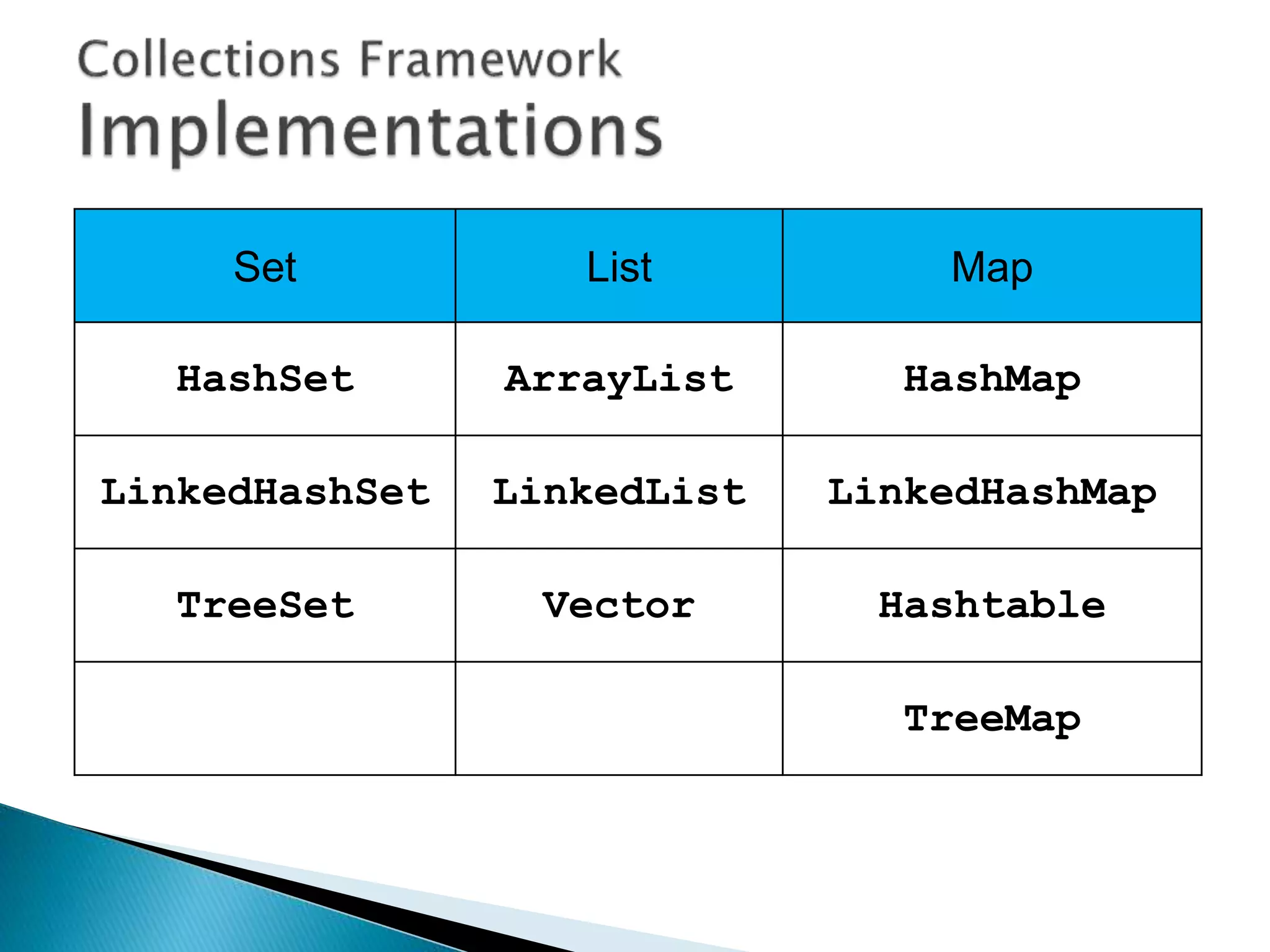
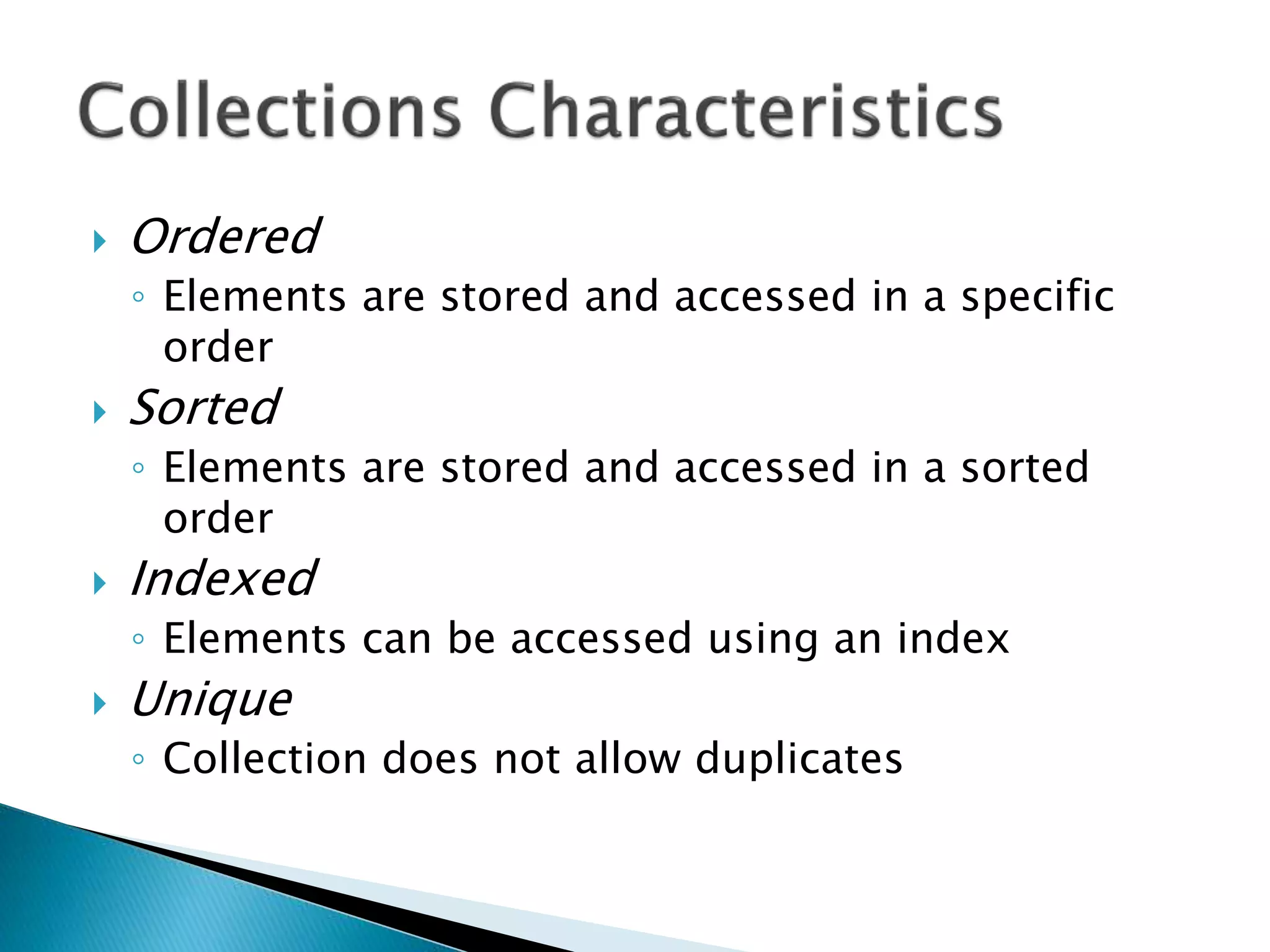
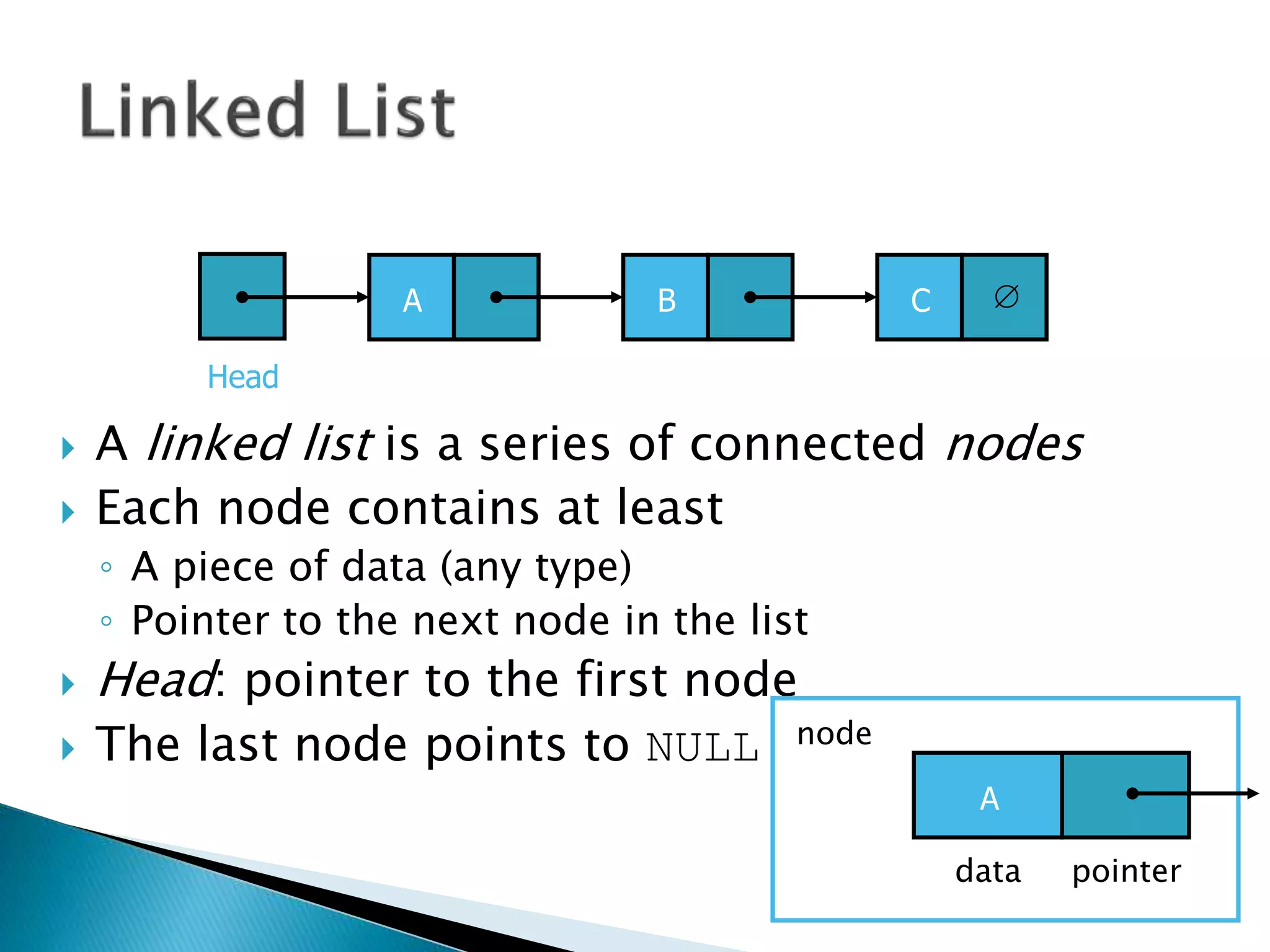
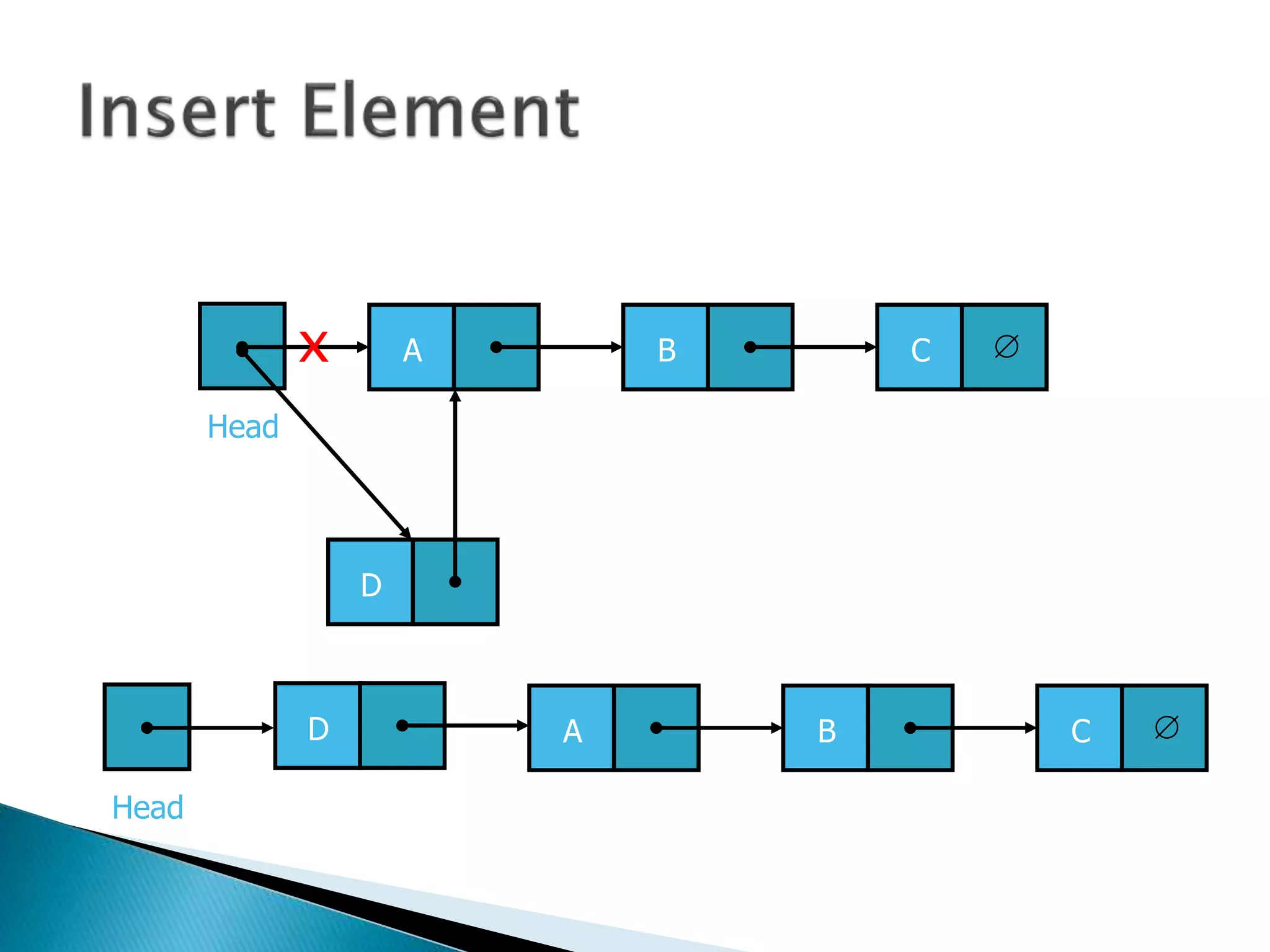
The document discusses algorithms and their analysis. It begins by defining an algorithm and key aspects like correctness, input, and output. It then discusses two aspects of algorithm performance - time and space. Examples are provided to illustrate how to analyze the time complexity of different structures like if/else statements, simple loops, and nested loops. Big O notation is introduced to describe an algorithm's growth rate. Common time complexities like constant, linear, quadratic, and cubic functions are defined. Specific sorting algorithms like insertion sort, selection sort, bubble sort, merge sort, and quicksort are then covered in detail with examples of how they work and their time complexities.


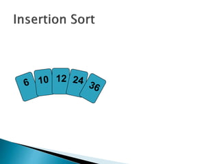
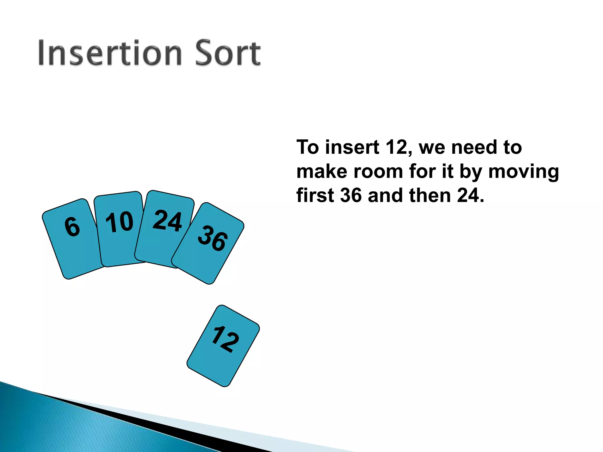
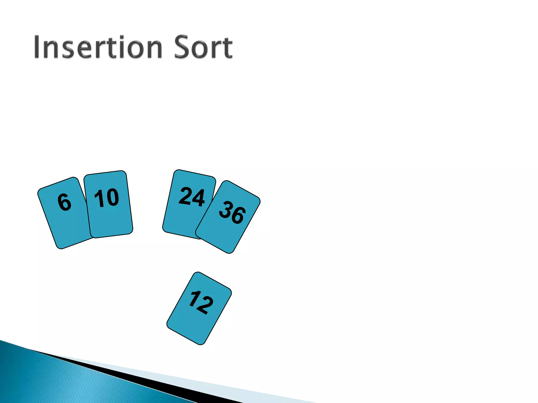
![insertionsort (a) {
for (i = 1; i < a.length; ++i) {
key = a[i]
pos = i
while (pos > 0 && a[pos-1] > key) {
a[pos]=a[pos-1]
pos--
}
a[pos] = key
}
}](https://image.slidesharecdn.com/algorithms-151215121740/85/Introduction-to-Algorithms-28-320.jpg)


![40 20 10 80 60 50 7 30 100pivot_index = 0
[0] [1] [2] [3] [4] [5] [6] [7] [8]
too_big_index too_small_index](https://image.slidesharecdn.com/algorithms-151215121740/85/Introduction-to-Algorithms-61-320.jpg)
![40 20 10 80 60 50 7 30 100pivot_index = 0
[0] [1] [2] [3] [4] [5] [6] [7] [8]
too_big_index too_small_index
1. while a[too_big_index] <= a[pivot_index]
++too_big_index](https://image.slidesharecdn.com/algorithms-151215121740/85/Introduction-to-Algorithms-62-320.jpg)
![40 20 10 80 60 50 7 30 100pivot_index = 0
[0] [1] [2] [3] [4] [5] [6] [7] [8]
too_big_index too_small_index
1. while a[too_big_index] <= a[pivot_index]
++too_big_index](https://image.slidesharecdn.com/algorithms-151215121740/85/Introduction-to-Algorithms-63-320.jpg)
![40 20 10 80 60 50 7 30 100pivot_index = 0
[0] [1] [2] [3] [4] [5] [6] [7] [8]
too_big_index too_small_index
1. while a[too_big_index] <= a[pivot_index]
++too_big_index](https://image.slidesharecdn.com/algorithms-151215121740/85/Introduction-to-Algorithms-64-320.jpg)
![40 20 10 80 60 50 7 30 100pivot_index = 0
[0] [1] [2] [3] [4] [5] [6] [7] [8]
too_big_index too_small_index
1. while a[too_big_index] <= a[pivot_index]
++too_big_index
2. while a[too_small_index] > a[pivot_index]
--too_small_index](https://image.slidesharecdn.com/algorithms-151215121740/85/Introduction-to-Algorithms-65-320.jpg)
![40 20 10 80 60 50 7 30 100pivot_index = 0
[0] [1] [2] [3] [4] [5] [6] [7] [8]
too_big_index too_small_index
1. while a[too_big_index] <= a[pivot_index]
++too_big_index
2. while a[too_small_index] > a[pivot_index]
--too_small_index](https://image.slidesharecdn.com/algorithms-151215121740/85/Introduction-to-Algorithms-66-320.jpg)
![40 20 10 80 60 50 7 30 100pivot_index = 0
[0] [1] [2] [3] [4] [5] [6] [7] [8]
too_big_index too_small_index
1. while a[too_big_index] <= a[pivot_index]
++too_big_index
2. while a[too_small_index] > a[pivot_index]
--too_small_index
3. if too_big_index < too_small_index
swap a[too_big_index]a[too_small_index]](https://image.slidesharecdn.com/algorithms-151215121740/85/Introduction-to-Algorithms-67-320.jpg)
![40 20 10 30 60 50 7 80 100pivot_index = 0
[0] [1] [2] [3] [4] [5] [6] [7] [8]
too_big_index too_small_index
1. while a[too_big_index] <= a[pivot_index]
++too_big_index
2. while a[too_small_index] > a[pivot_index]
--too_small_index
3. if too_big_index < too_small_index
swap a[too_big_index]a[too_small_index]](https://image.slidesharecdn.com/algorithms-151215121740/85/Introduction-to-Algorithms-68-320.jpg)
![40 20 10 30 60 50 7 80 100pivot_index = 0
[0] [1] [2] [3] [4] [5] [6] [7] [8]
too_big_index too_small_index
1. while a[too_big_index] <= a[pivot_index]
++too_big_index
2. while a[too_small_index] > a[pivot_index]
--too_small_index
3. if too_big_index < too_small_index
swap a[too_big_index]a[too_small_index]
4. while too_small_index > too_big_index, go to 1.](https://image.slidesharecdn.com/algorithms-151215121740/85/Introduction-to-Algorithms-69-320.jpg)
![40 20 10 30 60 50 7 80 100pivot_index = 0
[0] [1] [2] [3] [4] [5] [6] [7] [8]
too_big_index too_small_index
1. while a[too_big_index] <= a[pivot_index]
++too_big_index
2. while a[too_small_index] > a[pivot_index]
--too_small_index
3. if too_big_index < too_small_index
swap a[too_big_index]a[too_small_index]
4. while too_small_index > too_big_index, go to 1.](https://image.slidesharecdn.com/algorithms-151215121740/85/Introduction-to-Algorithms-70-320.jpg)
![40 20 10 30 60 50 7 80 100pivot_index = 0
[0] [1] [2] [3] [4] [5] [6] [7] [8]
too_big_index too_small_index
1. while a[too_big_index] <= a[pivot_index]
++too_big_index
2. while a[too_small_index] > a[pivot_index]
--too_small_index
3. if too_big_index < too_small_index
swap a[too_big_index]a[too_small_index]
4. while too_small_index > too_big_index, go to 1.](https://image.slidesharecdn.com/algorithms-151215121740/85/Introduction-to-Algorithms-71-320.jpg)
![40 20 10 30 60 50 7 80 100pivot_index = 0
[0] [1] [2] [3] [4] [5] [6] [7] [8]
too_big_index too_small_index
1. while a[too_big_index] <= a[pivot_index]
++too_big_index
2. while a[too_small_index] > a[pivot_index]
--too_small_index
3. if too_big_index < too_small_index
swap a[too_big_index]a[too_small_index]
4. while too_small_index > too_big_index, go to 1.](https://image.slidesharecdn.com/algorithms-151215121740/85/Introduction-to-Algorithms-72-320.jpg)
![40 20 10 30 60 50 7 80 100pivot_index = 0
[0] [1] [2] [3] [4] [5] [6] [7] [8]
too_big_index too_small_index
1. while a[too_big_index] <= a[pivot_index]
++too_big_index
2. while a[too_small_index] > a[pivot_index]
--too_small_index
3. if too_big_index < too_small_index
swap a[too_big_index]a[too_small_index]
4. while too_small_index > too_big_index, go to 1.](https://image.slidesharecdn.com/algorithms-151215121740/85/Introduction-to-Algorithms-73-320.jpg)
![40 20 10 30 60 50 7 80 100pivot_index = 0
[0] [1] [2] [3] [4] [5] [6] [7] [8]
too_big_index too_small_index
1. while a[too_big_index] <= a[pivot_index]
++too_big_index
2. while a[too_small_index] > a[pivot_index]
--too_small_index
3. if too_big_index < too_small_index
swap a[too_big_index]a[too_small_index]
4. while too_small_index > too_big_index, go to 1.](https://image.slidesharecdn.com/algorithms-151215121740/85/Introduction-to-Algorithms-74-320.jpg)
![40 20 10 30 7 50 60 80 100pivot_index = 0
[0] [1] [2] [3] [4] [5] [6] [7] [8]
too_big_index too_small_index
1. while a[too_big_index] <= a[pivot_index]
++too_big_index
2. while a[too_small_index] > a[pivot_index]
--too_small_index
3. if too_big_index < too_small_index
swap a[too_big_index]a[too_small_index]
4. while too_small_index > too_big_index, go to 1.](https://image.slidesharecdn.com/algorithms-151215121740/85/Introduction-to-Algorithms-75-320.jpg)
![40 20 10 30 7 50 60 80 100pivot_index = 0
[0] [1] [2] [3] [4] [5] [6] [7] [8]
too_big_index too_small_index
1. while a[too_big_index] <= a[pivot_index]
++too_big_index
2. while a[too_small_index] > a[pivot_index]
--too_small_index
3. if too_big_index < too_small_index
swap a[too_big_index]a[too_small_index]
4. while too_small_index > too_big_index, go to 1.](https://image.slidesharecdn.com/algorithms-151215121740/85/Introduction-to-Algorithms-76-320.jpg)
![40 20 10 30 7 50 60 80 100pivot_index = 0
[0] [1] [2] [3] [4] [5] [6] [7] [8]
too_big_index too_small_index
1. while a[too_big_index] <= a[pivot_index]
++too_big_index
2. while a[too_small_index] > a[pivot_index]
--too_small_index
3. if too_big_index < too_small_index
swap a[too_big_index]a[too_small_index]
4. while too_small_index > too_big_index, go to 1.](https://image.slidesharecdn.com/algorithms-151215121740/85/Introduction-to-Algorithms-77-320.jpg)
![40 20 10 30 7 50 60 80 100pivot_index = 0
[0] [1] [2] [3] [4] [5] [6] [7] [8]
too_big_index too_small_index
1. while a[too_big_index] <= a[pivot_index]
++too_big_index
2. while a[too_small_index] > a[pivot_index]
--too_small_index
3. if too_big_index < too_small_index
swap a[too_big_index]a[too_small_index]
4. while too_small_index > too_big_index, go to 1.](https://image.slidesharecdn.com/algorithms-151215121740/85/Introduction-to-Algorithms-78-320.jpg)
![40 20 10 30 7 50 60 80 100pivot_index = 0
[0] [1] [2] [3] [4] [5] [6] [7] [8]
too_big_index too_small_index
1. while a[too_big_index] <= a[pivot_index]
++too_big_index
2. while a[too_small_index] > a[pivot_index]
--too_small_index
3. if too_big_index < too_small_index
swap a[too_big_index]a[too_small_index]
4. while too_small_index > too_big_index, go to 1.](https://image.slidesharecdn.com/algorithms-151215121740/85/Introduction-to-Algorithms-79-320.jpg)
![40 20 10 30 7 50 60 80 100pivot_index = 0
[0] [1] [2] [3] [4] [5] [6] [7] [8]
too_big_index too_small_index
1. while a[too_big_index] <= a[pivot_index]
++too_big_index
2. while a[too_small_index] > a[pivot_index]
--too_small_index
3. if too_big_index < too_small_index
swap a[too_big_index]a[too_small_index]
4. while too_small_index > too_big_index, go to 1.](https://image.slidesharecdn.com/algorithms-151215121740/85/Introduction-to-Algorithms-80-320.jpg)
![40 20 10 30 7 50 60 80 100pivot_index = 0
[0] [1] [2] [3] [4] [5] [6] [7] [8]
too_big_index too_small_index
1. while a[too_big_index] <= a[pivot_index]
++too_big_index
2. while a[too_small_index] > a[pivot_index]
--too_small_index
3. if too_big_index < too_small_index
swap a[too_big_index]a[too_small_index]
4. while too_small_index > too_big_index, go to 1.](https://image.slidesharecdn.com/algorithms-151215121740/85/Introduction-to-Algorithms-81-320.jpg)
![40 20 10 30 7 50 60 80 100pivot_index = 0
[0] [1] [2] [3] [4] [5] [6] [7] [8]
too_big_index too_small_index
1. while a[too_big_index] <= a[pivot_index]
++too_big_index
2. while a[too_small_index] > a[pivot_index]
--too_small_index
3. if too_big_index < too_small_index
swap a[too_big_index]a[too_small_index]
4. while too_small_index > too_big_index, go to 1.](https://image.slidesharecdn.com/algorithms-151215121740/85/Introduction-to-Algorithms-82-320.jpg)
![40 20 10 30 7 50 60 80 100pivot_index = 0
[0] [1] [2] [3] [4] [5] [6] [7] [8]
too_big_index too_small_index
1. while a[too_big_index] <= a[pivot_index]
++too_big_index
2. while a[too_small_index] > a[pivot_index]
--too_small_index
3. if too_big_index < too_small_index
swap a[too_big_index]a[too_small_index]
4. while too_small_index > too_big_index, go to 1.](https://image.slidesharecdn.com/algorithms-151215121740/85/Introduction-to-Algorithms-83-320.jpg)
![1. while a[too_big_index] <= a[pivot_index]
++too_big_index
2. while a[too_small_index] > a[pivot_index]
--too_small_index
3. if too_big_index < too_small_index
swap a[too_big_index]a[too_small_index]
4. while too_small_index > too_big_index, go to 1.
5. swap a[too_small_index]a[pivot_index]
40 20 10 30 7 50 60 80 100pivot_index = 0
[0] [1] [2] [3] [4] [5] [6] [7] [8]
too_big_index too_small_index](https://image.slidesharecdn.com/algorithms-151215121740/85/Introduction-to-Algorithms-84-320.jpg)
![7 20 10 30 40 50 60 80 100pivot_index = 4
[0] [1] [2] [3] [4] [5] [6] [7] [8]
too_big_index too_small_index
1. while a[too_big_index] <= a[pivot_index]
++too_big_index
2. while a[too_small_index] > a[pivot_index]
--too_small_index
3. if too_big_index < too_small_index
swap a[too_big_index]a[too_small_index]
4. while too_small_index > too_big_index, go to 1.
5. swap a[too_small_index]a[pivot_index]](https://image.slidesharecdn.com/algorithms-151215121740/85/Introduction-to-Algorithms-85-320.jpg)

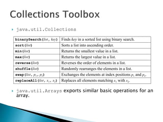
![Arrays methods:
public static void sort (int[] a)
public static void sort (Object[] a)
// requires Comparable
public static <T> void sort (T[] a,
Comparator<? super T> comp)
// uses given Comparator](https://image.slidesharecdn.com/algorithms-151215121740/85/Introduction-to-Algorithms-90-320.jpg)


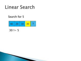
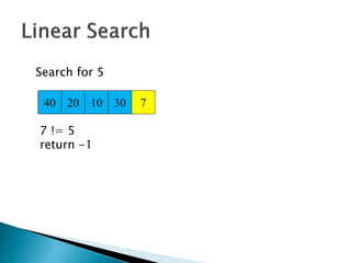
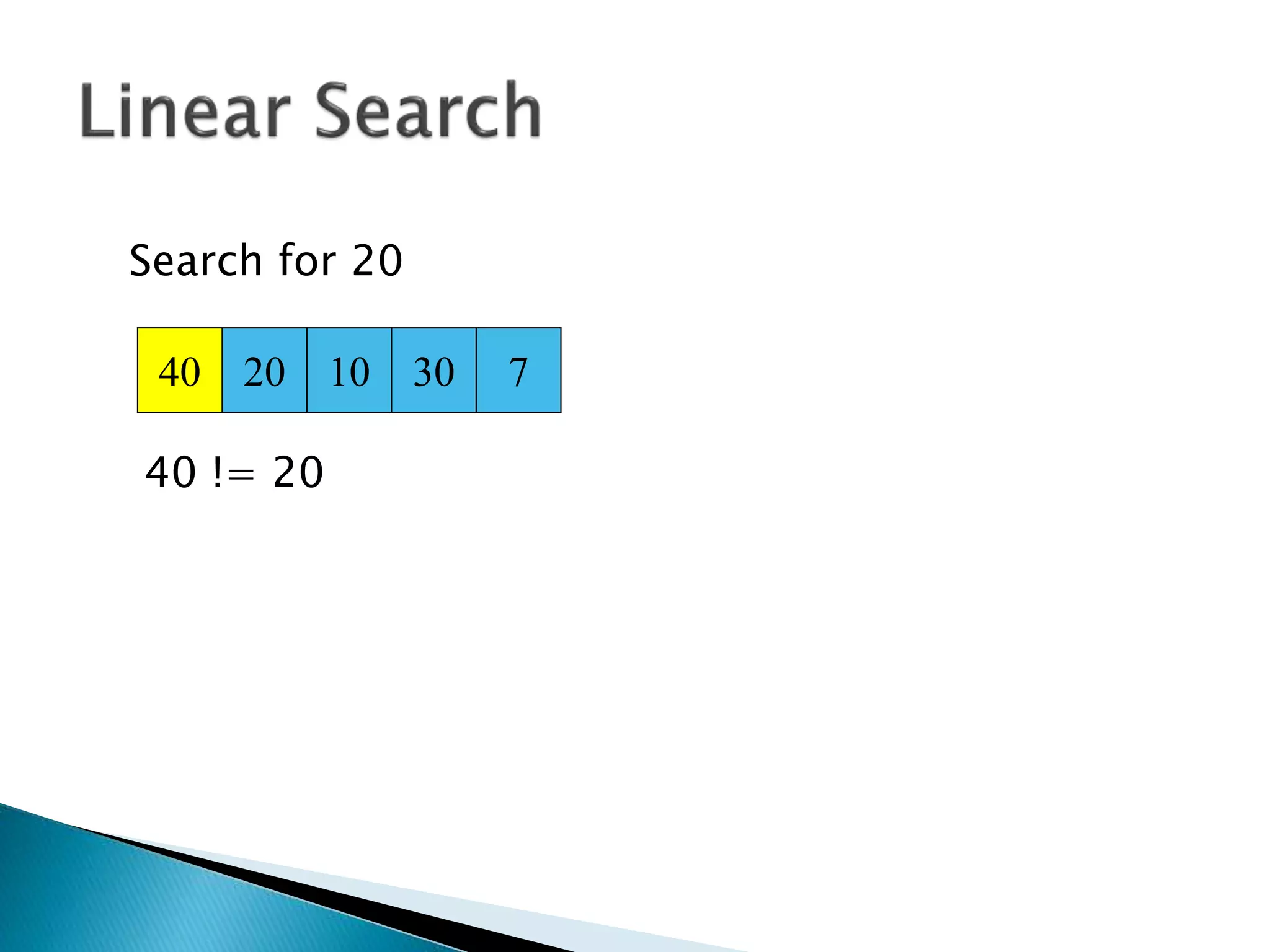
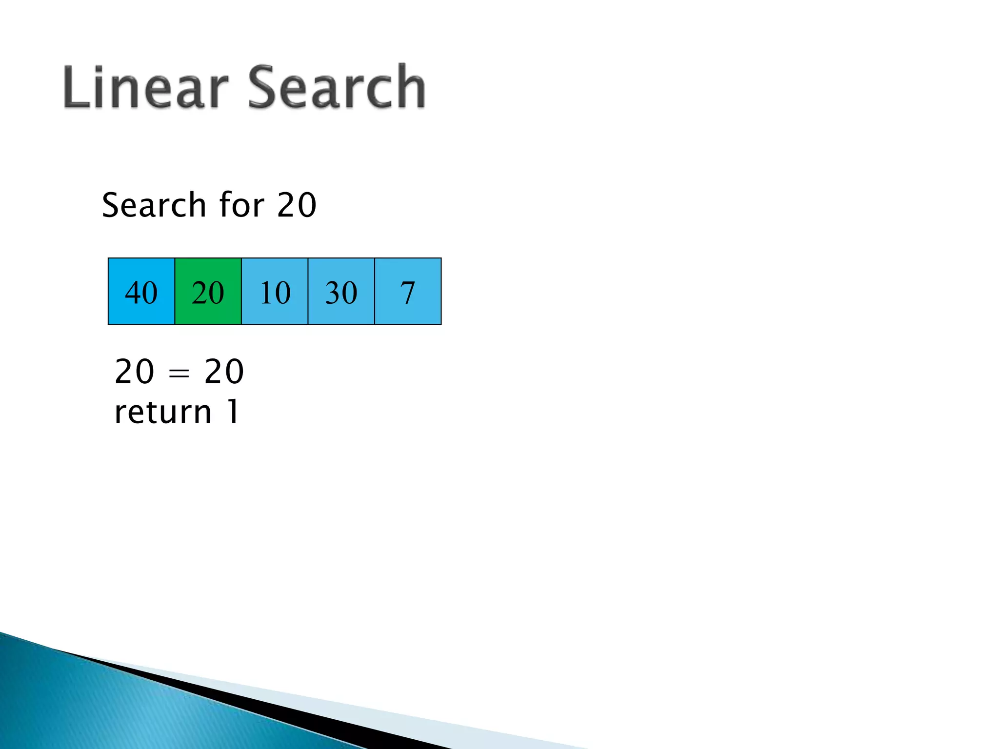
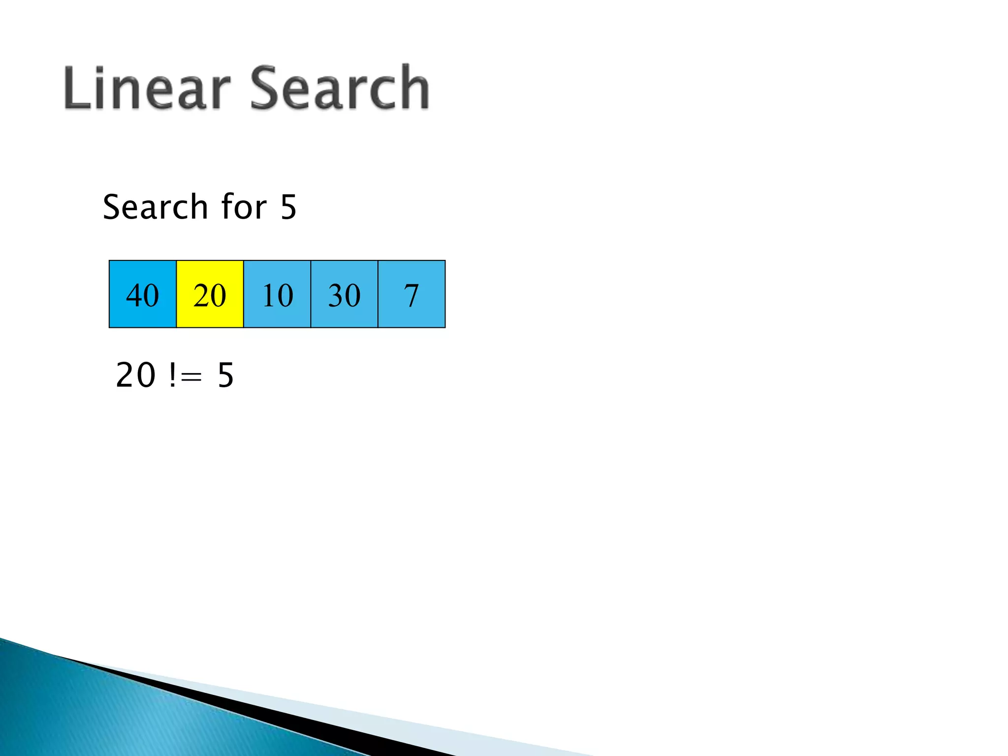
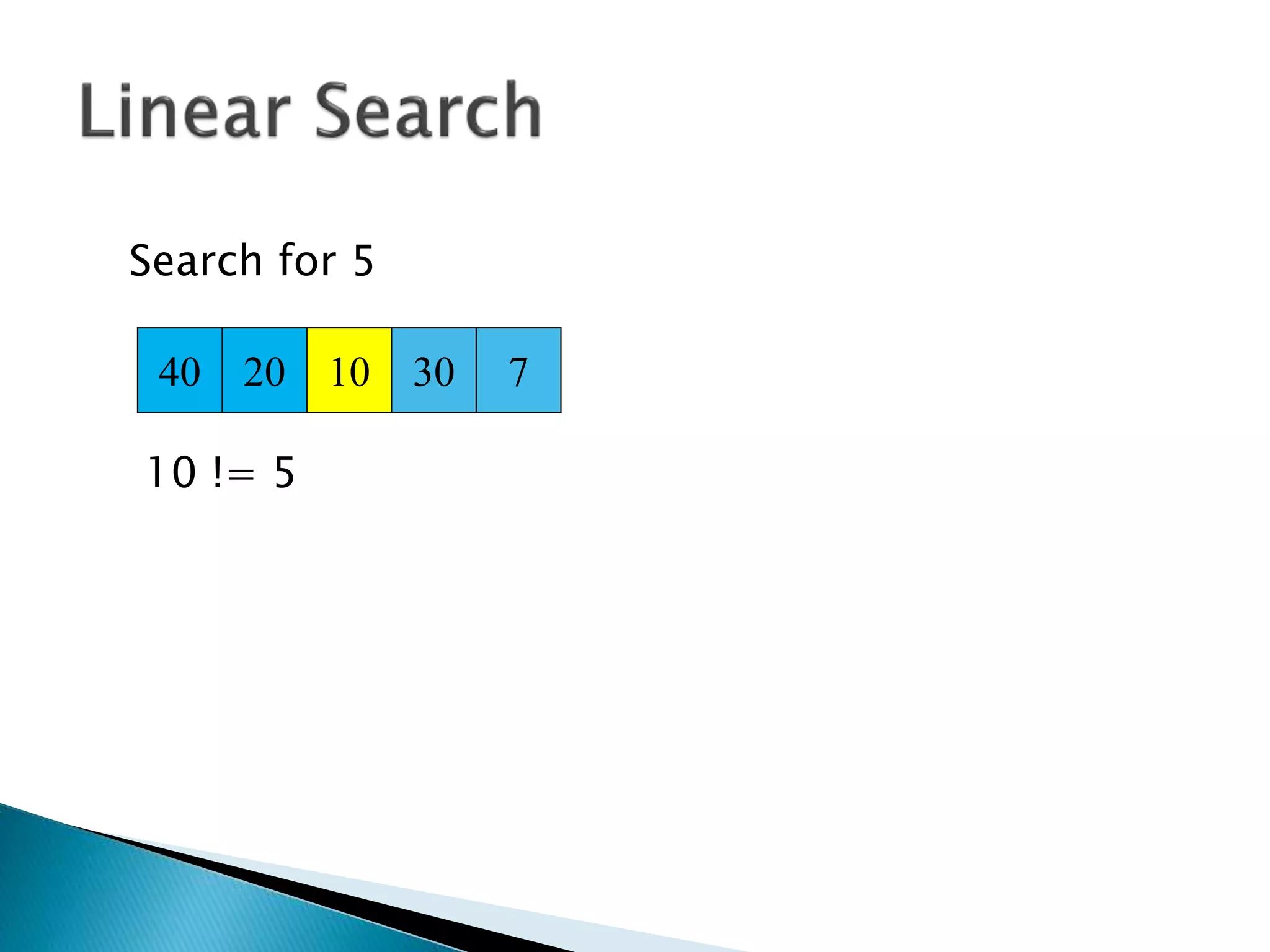
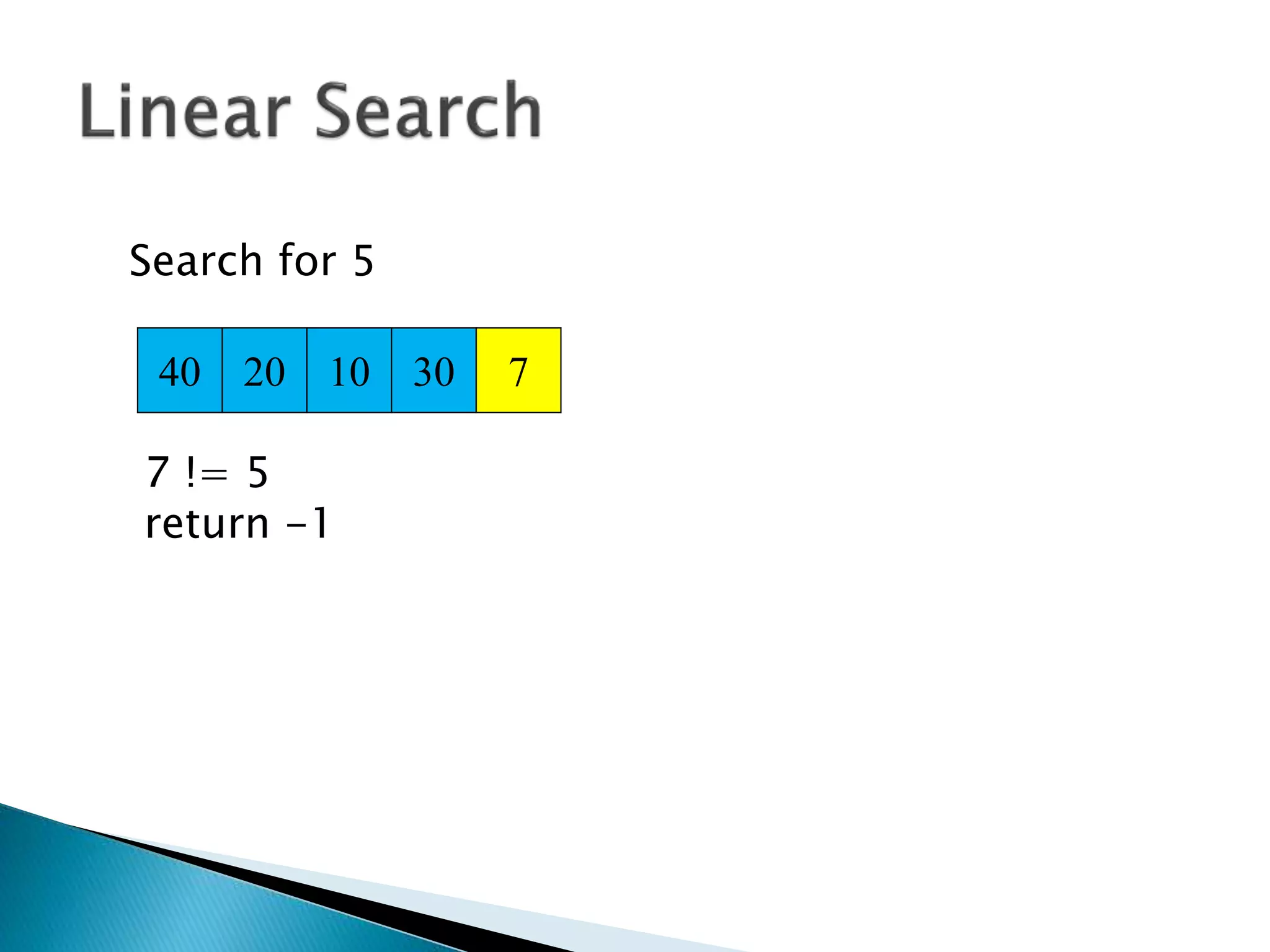
![linearsearch (a, key) {
for (i = 0; i < a.length; i++) {
if (a[i] == key) return i
}
return –1
}](https://image.slidesharecdn.com/algorithms-151215121740/85/Introduction-to-Algorithms-95-320.jpg)


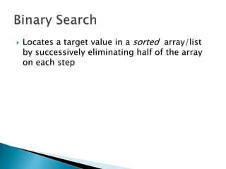
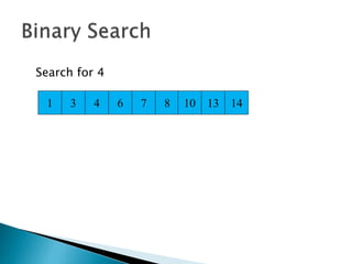
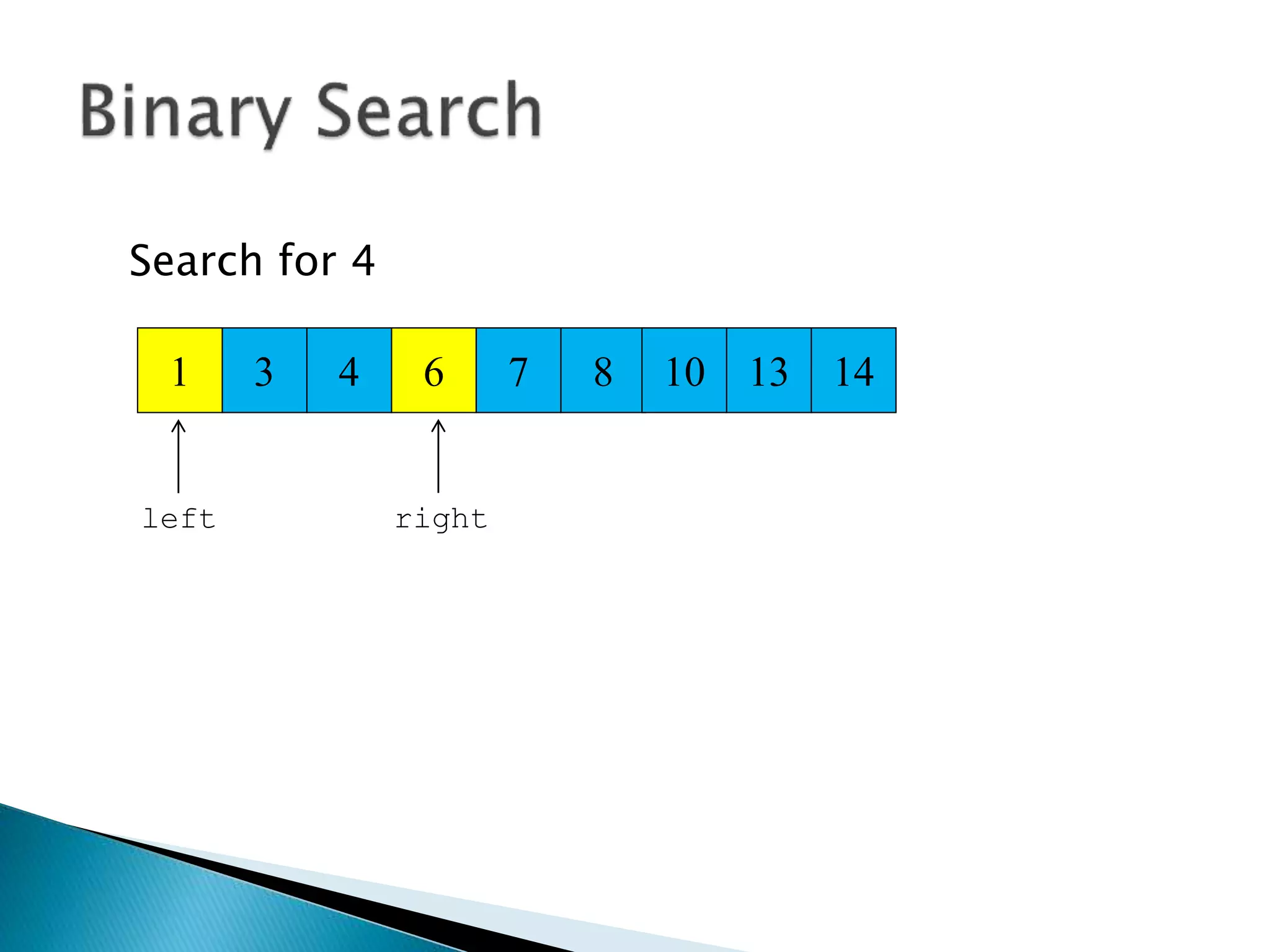
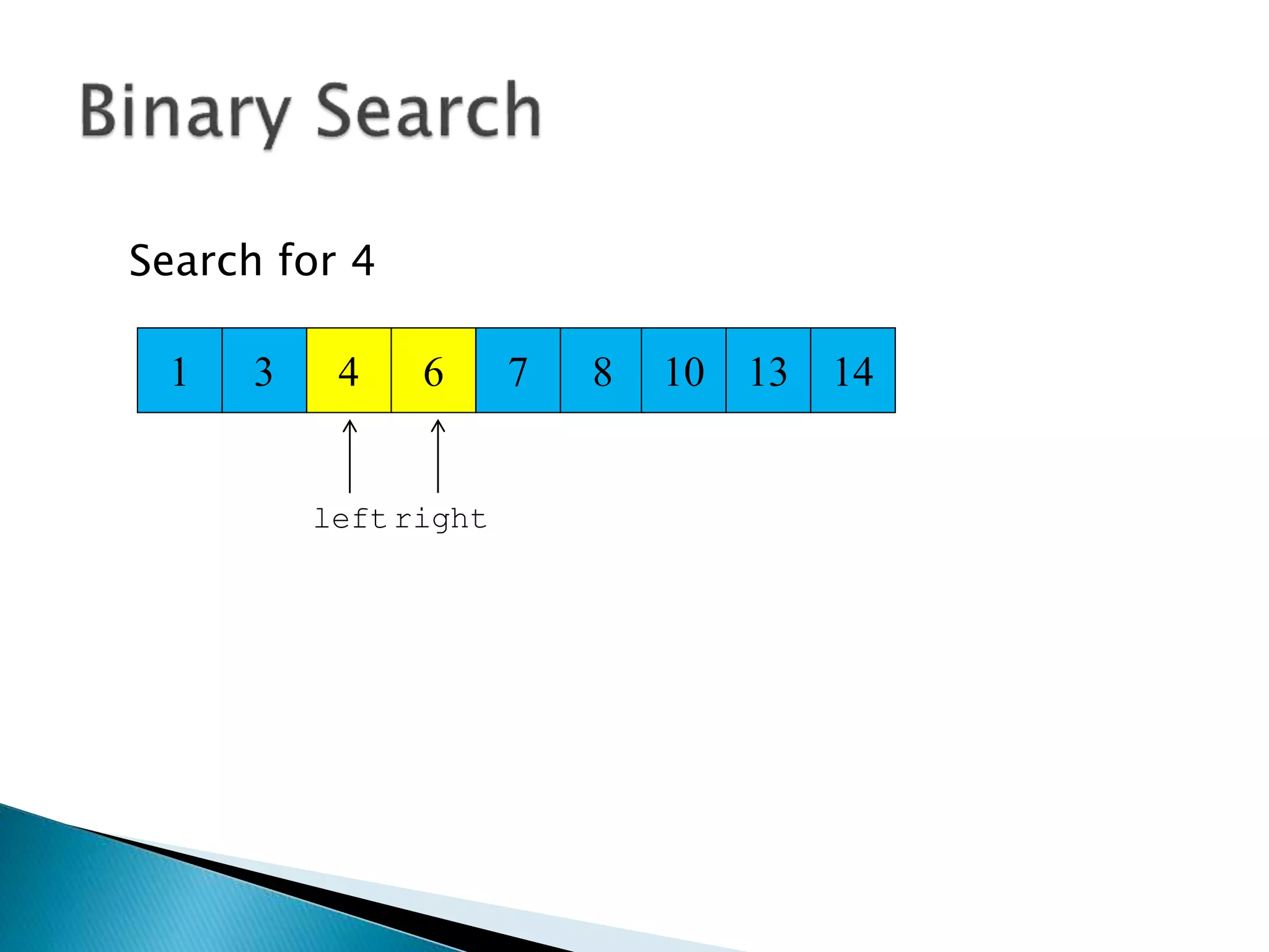
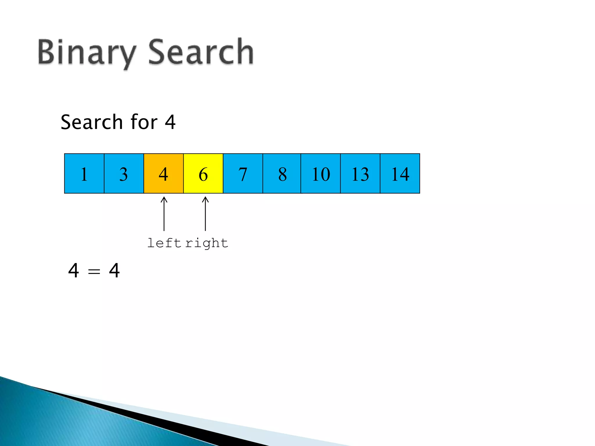
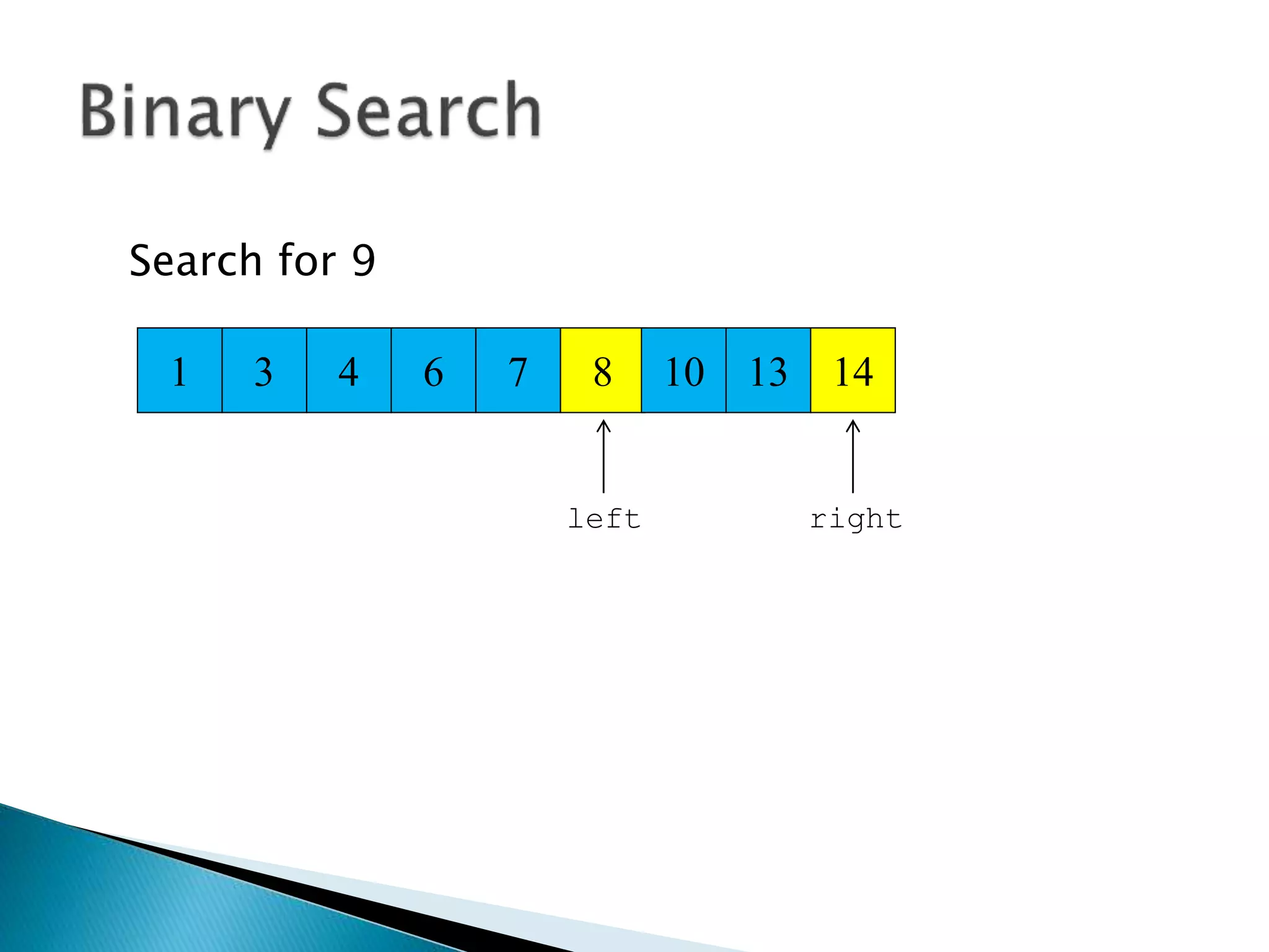
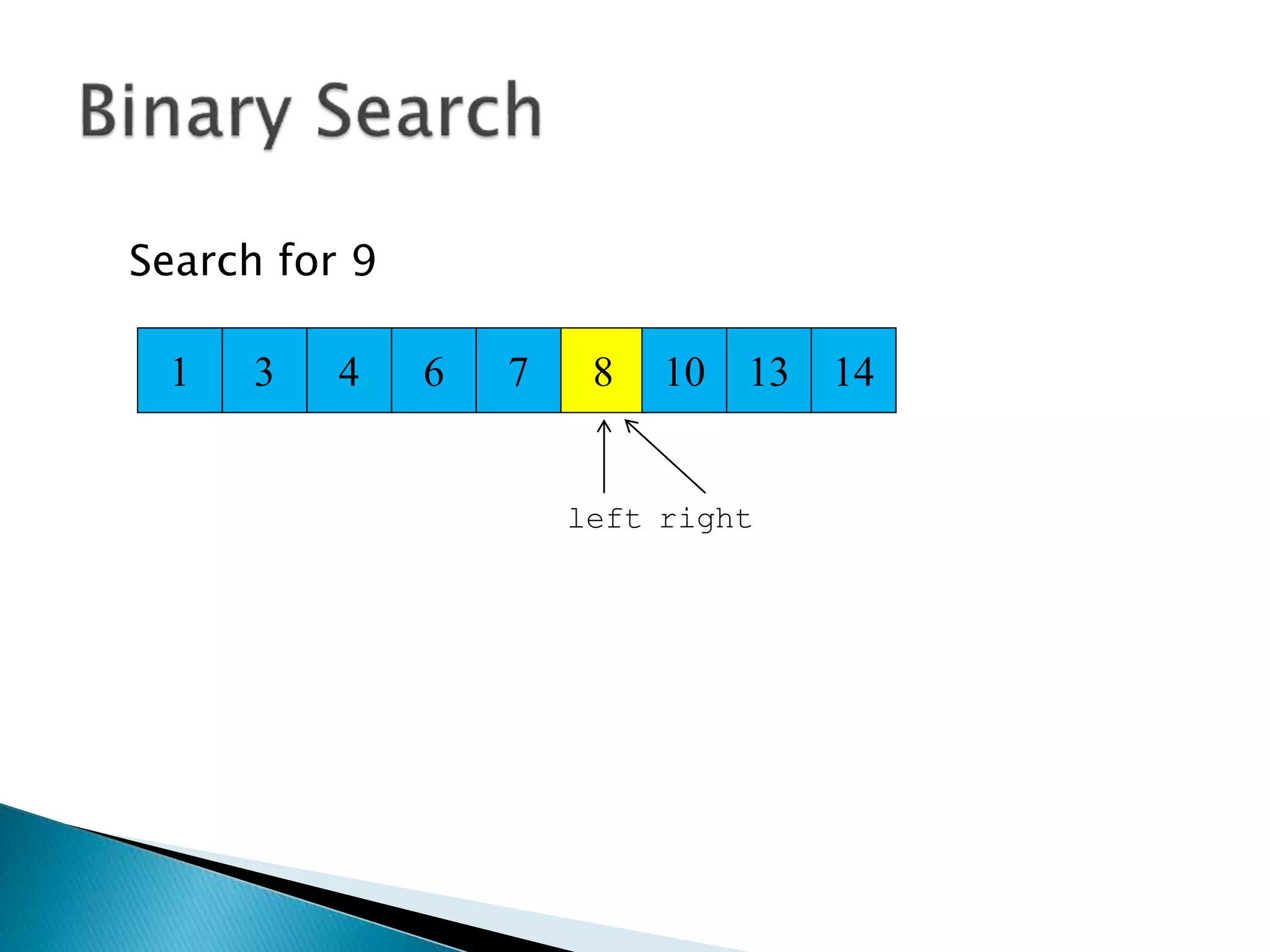
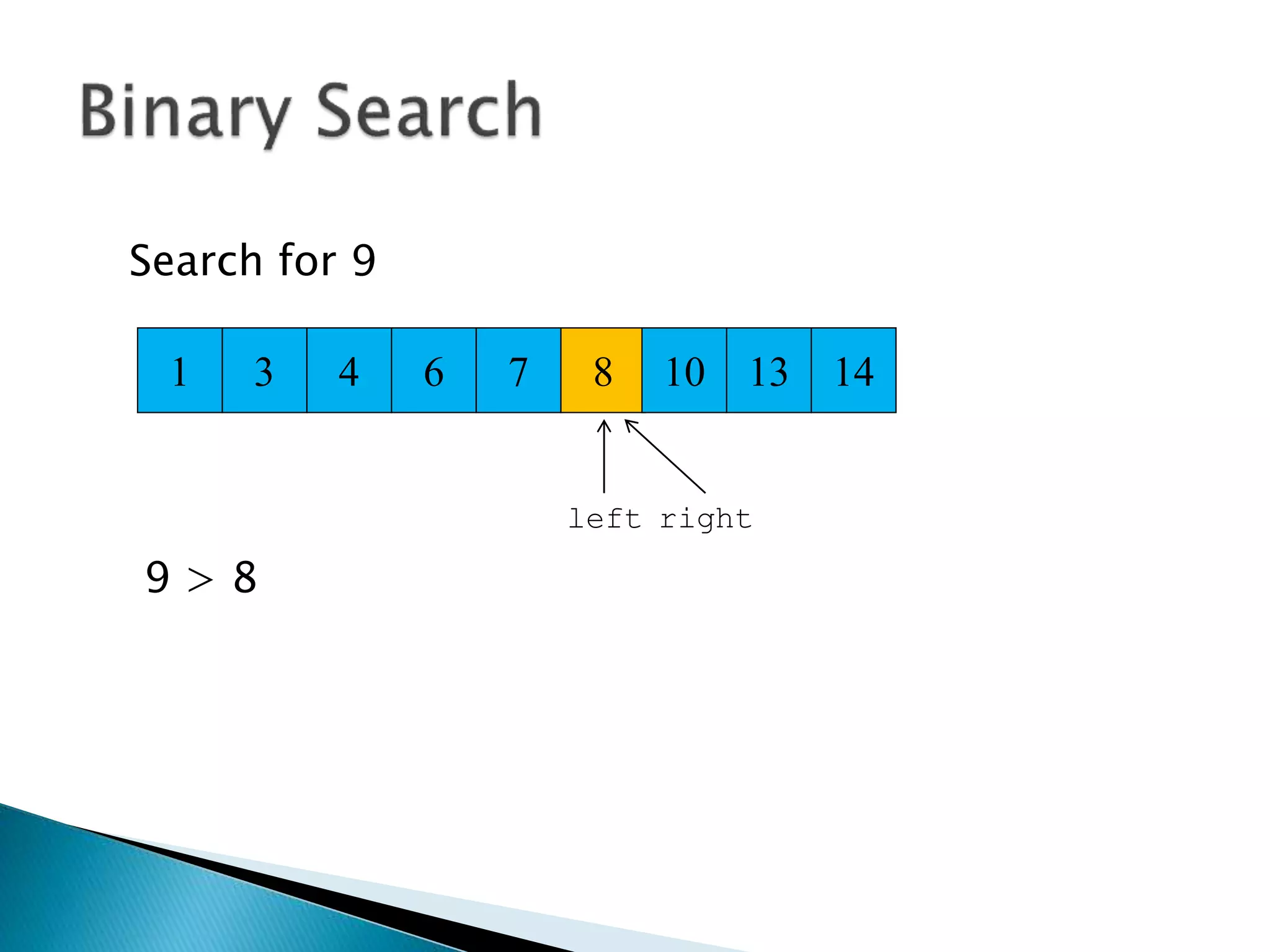
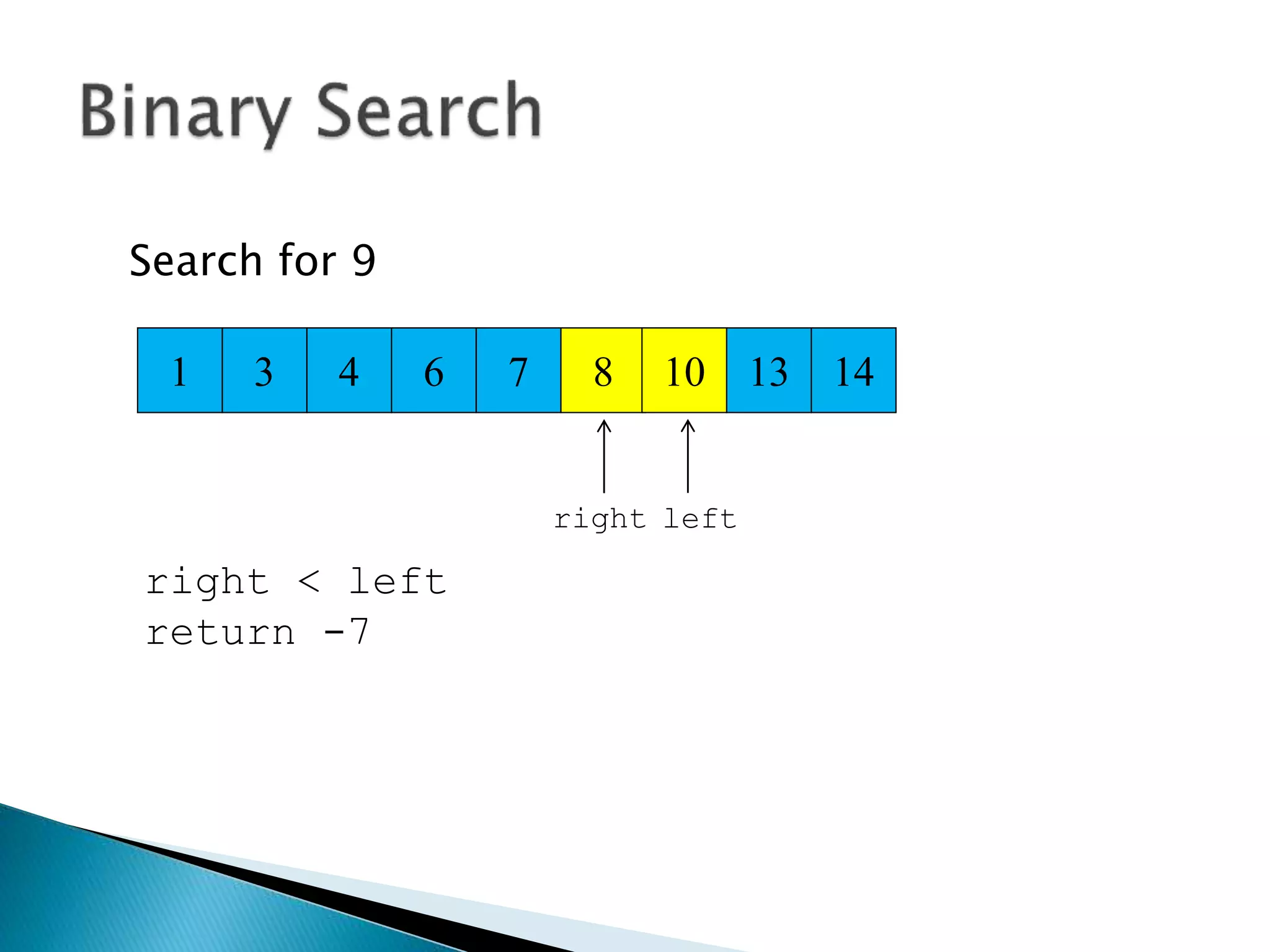
![binarysearch (a, low, high, key) {
while (low <= high) {
mid = (low+high) >>> 1
midVal = a[mid]
if (midVal < key) low=mid+1
else if (midVal > key) high=mid+1
else return mid
}
return –(low + 1)
}](https://image.slidesharecdn.com/algorithms-151215121740/85/Introduction-to-Algorithms-108-320.jpg)


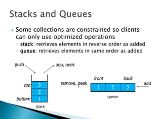
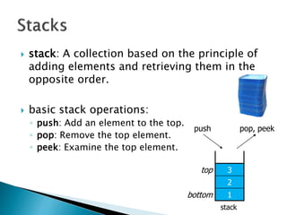
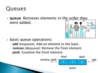
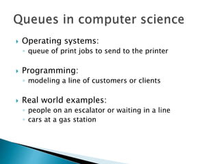
![ Programming languages and compilers:
◦ method call stack
Matching up related pairs of things:
◦ check correctness of brackets (){}[]
Sophisticated algorithms:
◦ undo stack](https://image.slidesharecdn.com/algorithms-151215121740/85/Introduction-to-Algorithms-142-320.jpg)


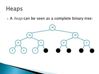
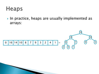
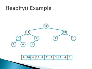
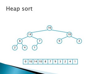
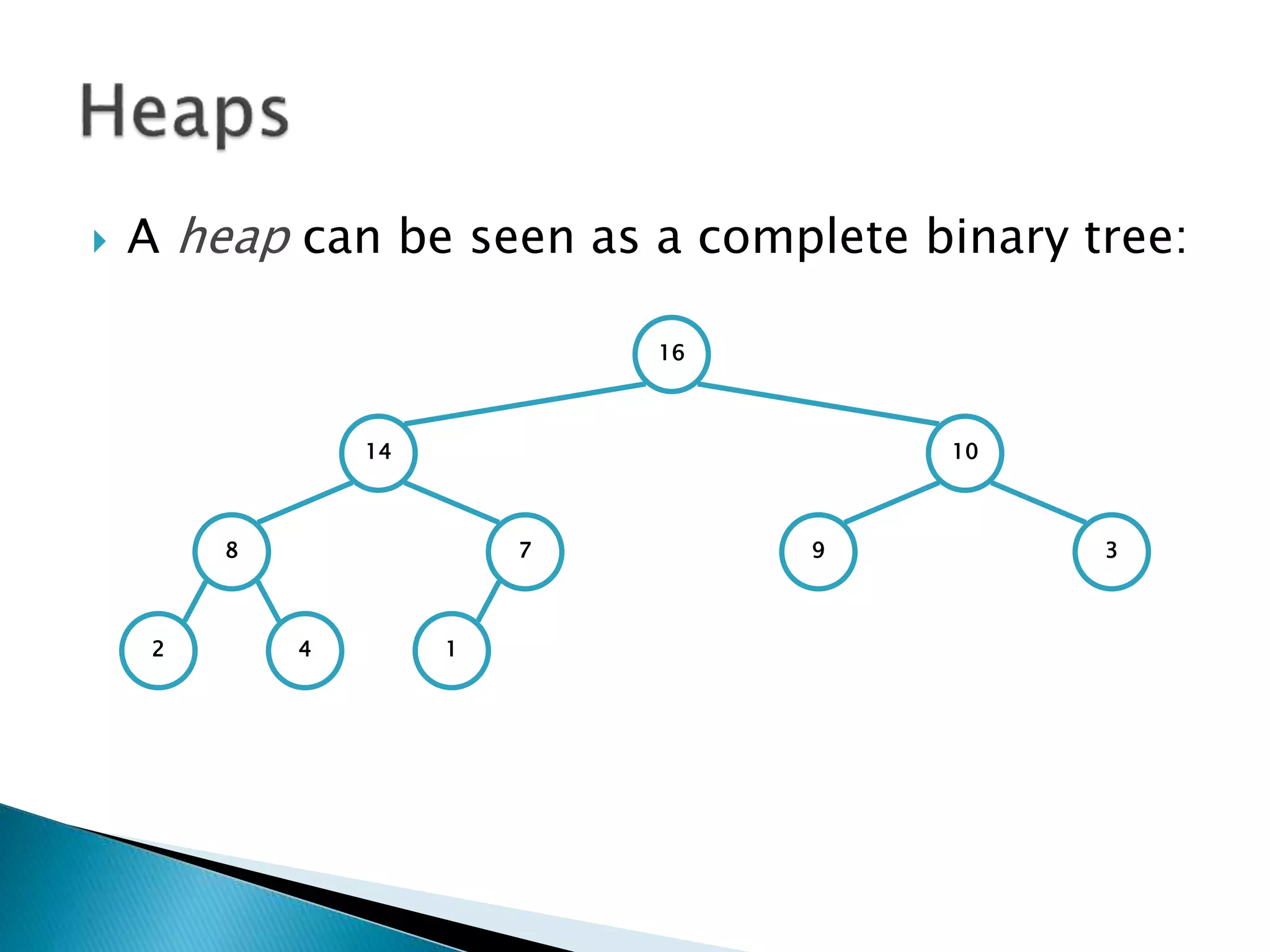
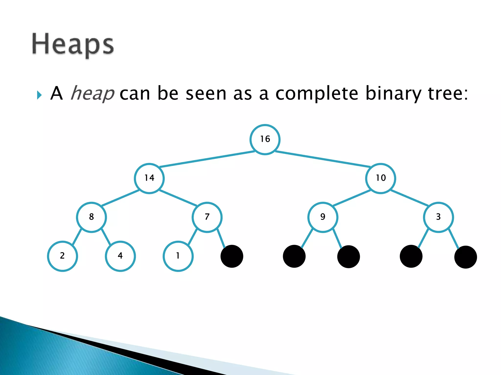
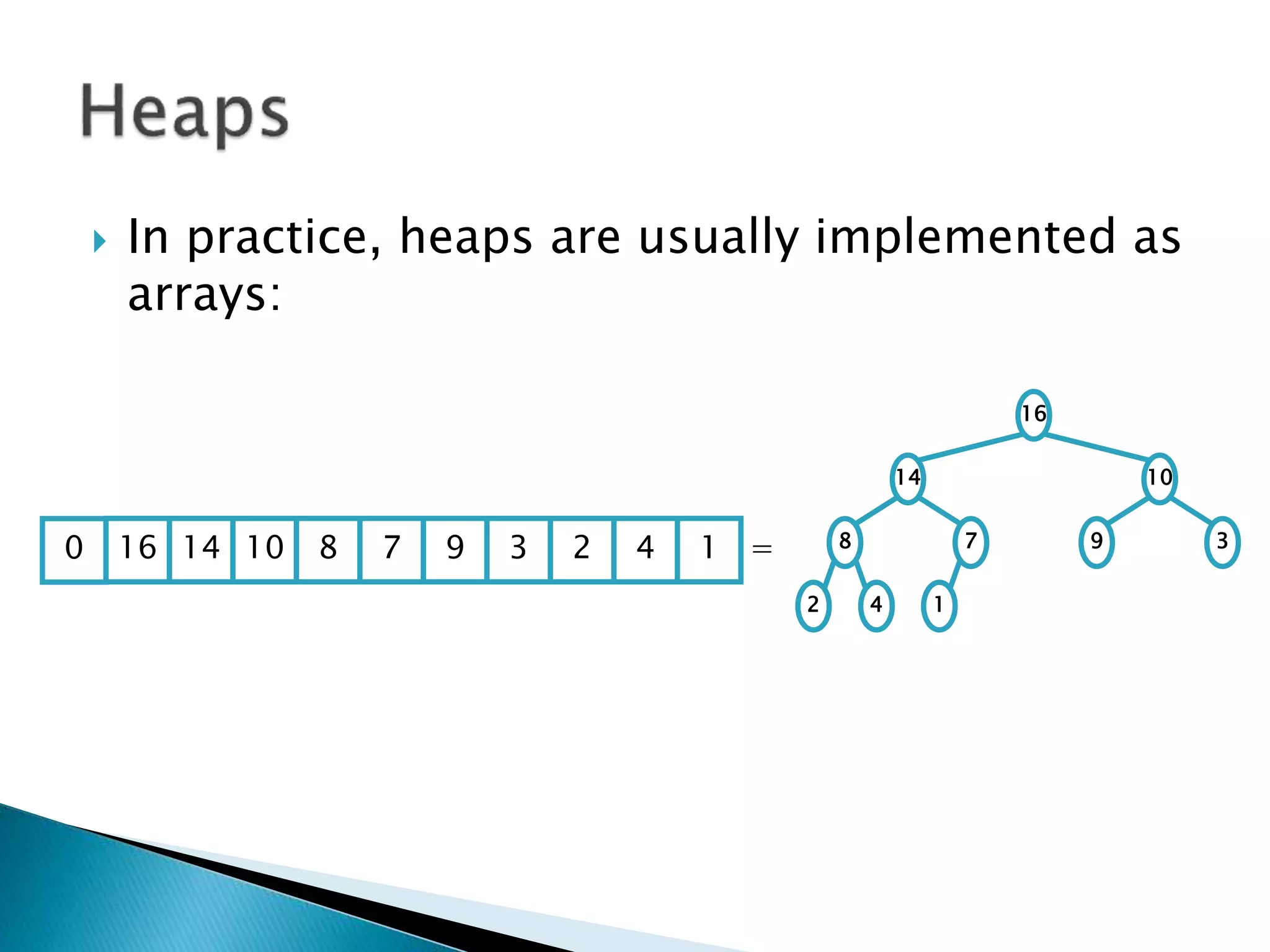
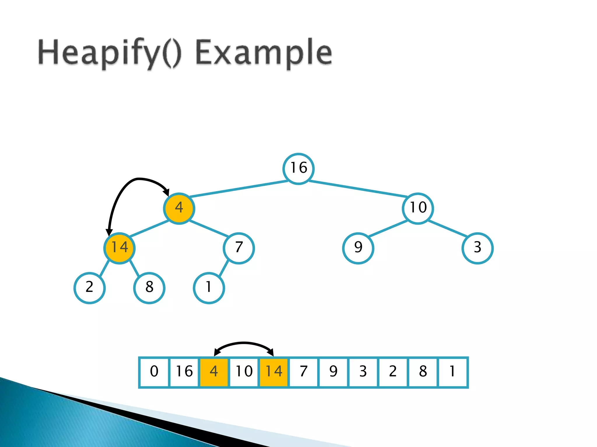
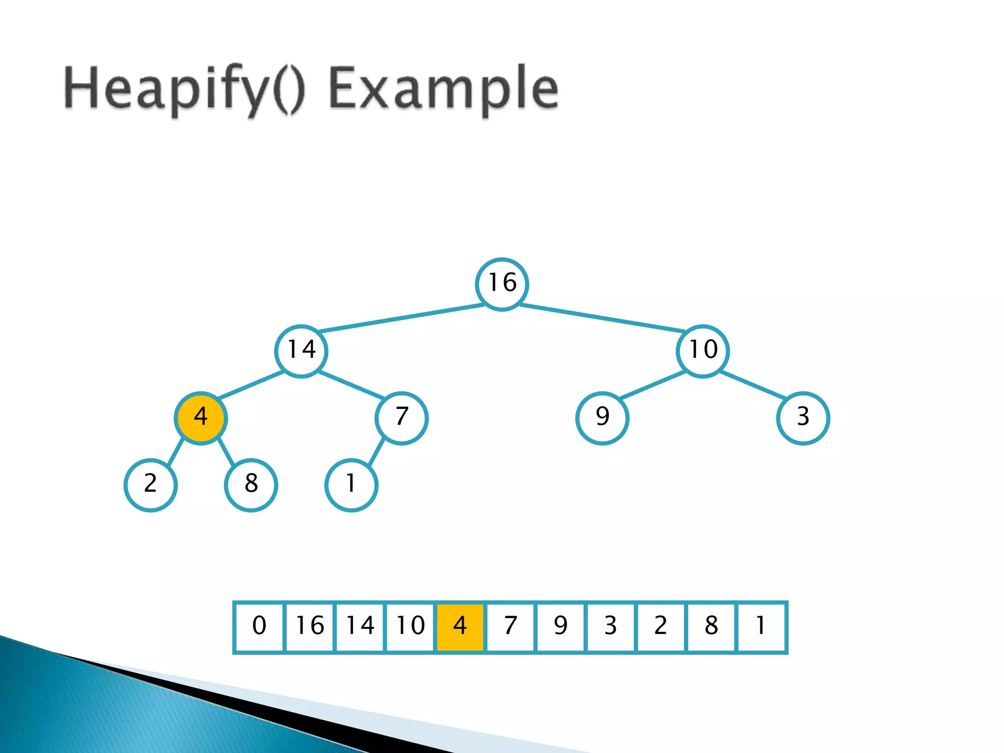
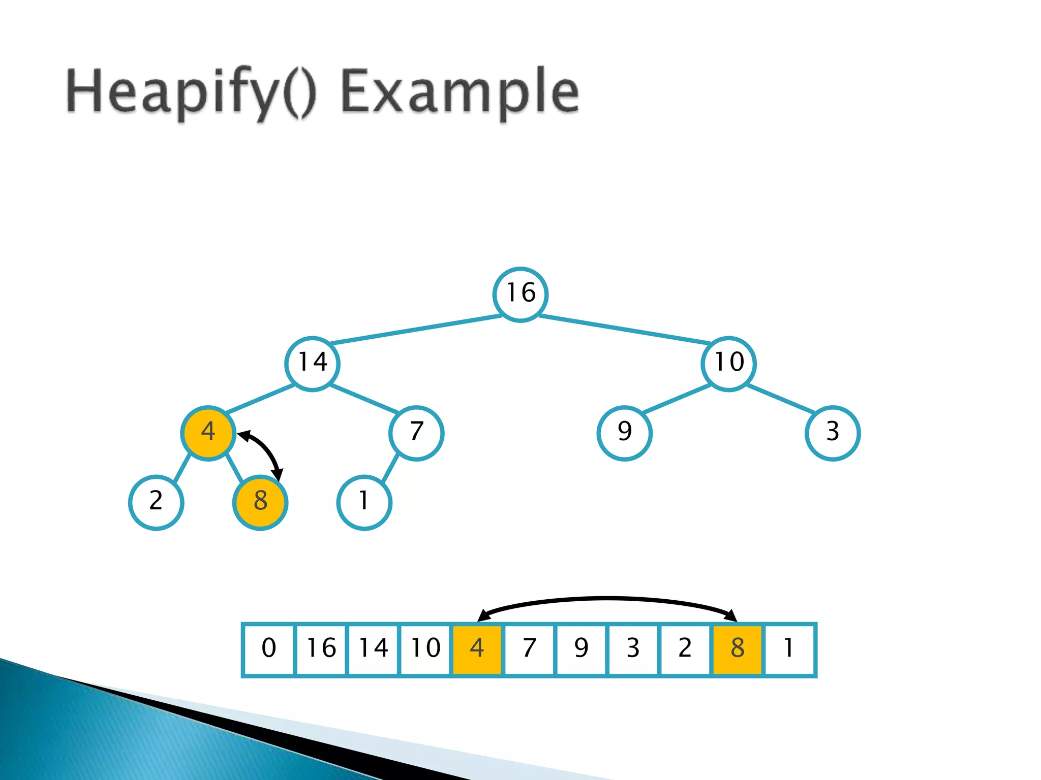
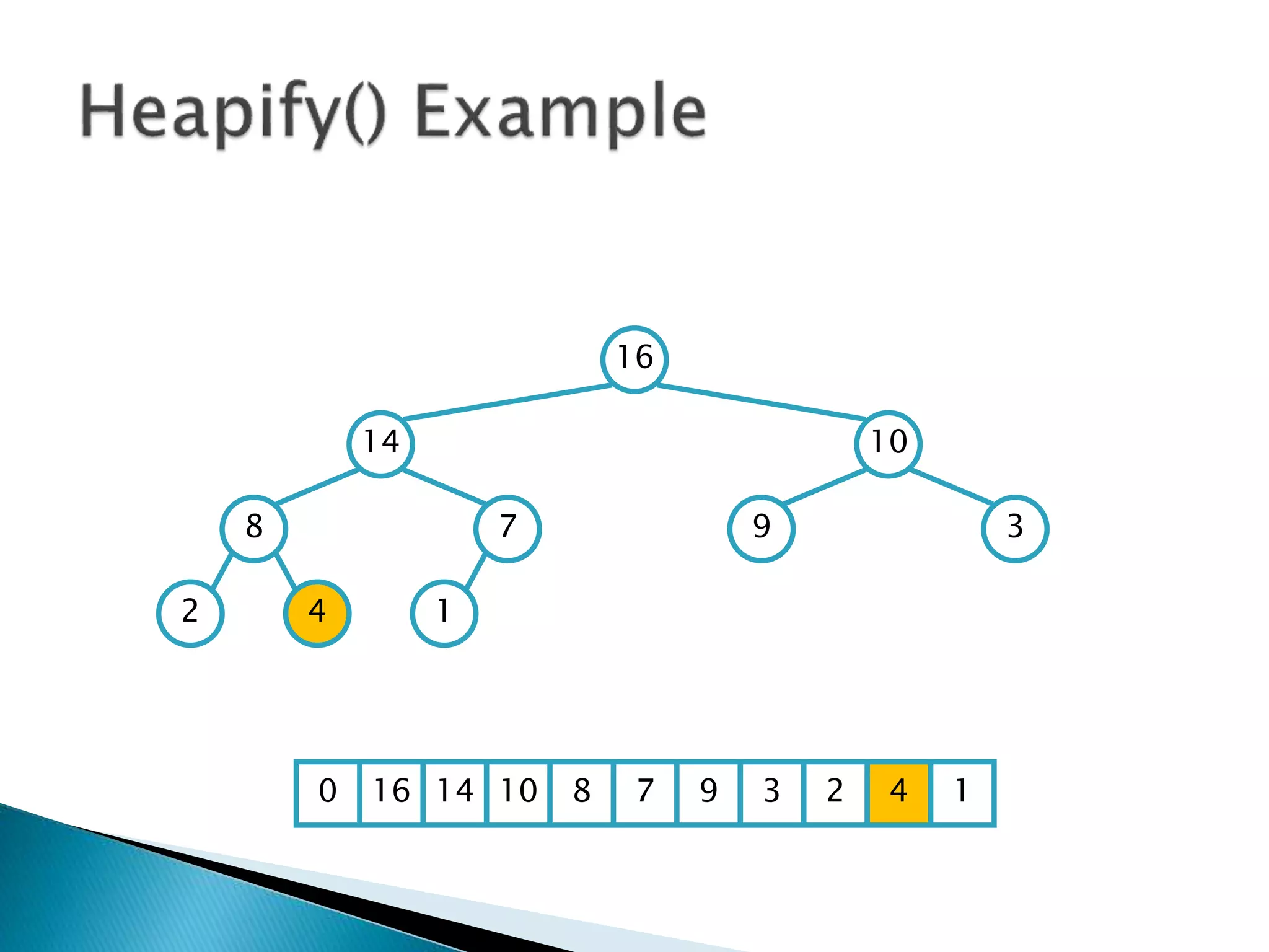
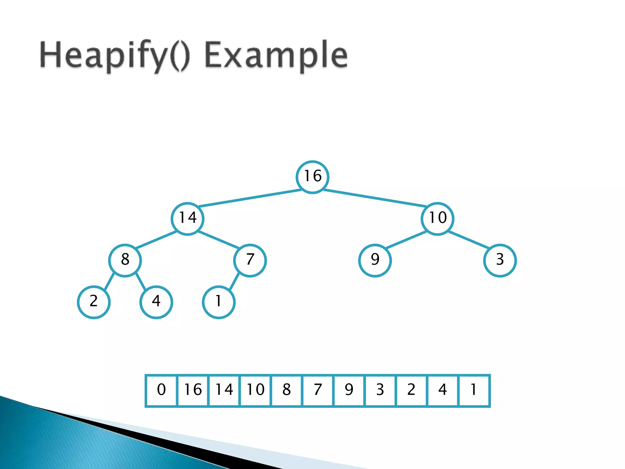
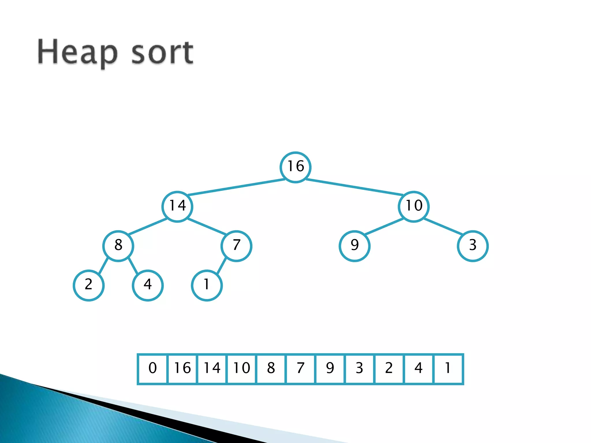
![ To represent a complete binary tree as an
array:
◦ The root node is A[1]
◦ Node i is A[i]
◦ The parent of node i is A[i/2] (note: integer divide)
◦ The left child of node i is A[2i]
◦ The right child of node i is A[2i + 1]
16
14 10
8 7 9 3
2 4 1
16 14 10 8 7 9 3 2 4 1 =0](https://image.slidesharecdn.com/algorithms-151215121740/85/Introduction-to-Algorithms-158-320.jpg)


![insertionsort (a) {
for (i = 1; i < a.length; ++i) {
key = a[i]
pos = i
while (pos > 0 && a[pos-1] > key) {
a[pos]=a[pos-1]
pos--
}
a[pos] = key
}
}](https://image.slidesharecdn.com/algorithms-151215121740/75/Introduction-to-Algorithms-28-2048.jpg)


![40 20 10 80 60 50 7 30 100pivot_index = 0
[0] [1] [2] [3] [4] [5] [6] [7] [8]
too_big_index too_small_index](https://image.slidesharecdn.com/algorithms-151215121740/75/Introduction-to-Algorithms-61-2048.jpg)
![40 20 10 80 60 50 7 30 100pivot_index = 0
[0] [1] [2] [3] [4] [5] [6] [7] [8]
too_big_index too_small_index
1. while a[too_big_index] <= a[pivot_index]
++too_big_index](https://image.slidesharecdn.com/algorithms-151215121740/75/Introduction-to-Algorithms-62-2048.jpg)
![40 20 10 80 60 50 7 30 100pivot_index = 0
[0] [1] [2] [3] [4] [5] [6] [7] [8]
too_big_index too_small_index
1. while a[too_big_index] <= a[pivot_index]
++too_big_index](https://image.slidesharecdn.com/algorithms-151215121740/75/Introduction-to-Algorithms-63-2048.jpg)
![40 20 10 80 60 50 7 30 100pivot_index = 0
[0] [1] [2] [3] [4] [5] [6] [7] [8]
too_big_index too_small_index
1. while a[too_big_index] <= a[pivot_index]
++too_big_index](https://image.slidesharecdn.com/algorithms-151215121740/75/Introduction-to-Algorithms-64-2048.jpg)
![40 20 10 80 60 50 7 30 100pivot_index = 0
[0] [1] [2] [3] [4] [5] [6] [7] [8]
too_big_index too_small_index
1. while a[too_big_index] <= a[pivot_index]
++too_big_index
2. while a[too_small_index] > a[pivot_index]
--too_small_index](https://image.slidesharecdn.com/algorithms-151215121740/75/Introduction-to-Algorithms-65-2048.jpg)
![40 20 10 80 60 50 7 30 100pivot_index = 0
[0] [1] [2] [3] [4] [5] [6] [7] [8]
too_big_index too_small_index
1. while a[too_big_index] <= a[pivot_index]
++too_big_index
2. while a[too_small_index] > a[pivot_index]
--too_small_index](https://image.slidesharecdn.com/algorithms-151215121740/75/Introduction-to-Algorithms-66-2048.jpg)
![40 20 10 80 60 50 7 30 100pivot_index = 0
[0] [1] [2] [3] [4] [5] [6] [7] [8]
too_big_index too_small_index
1. while a[too_big_index] <= a[pivot_index]
++too_big_index
2. while a[too_small_index] > a[pivot_index]
--too_small_index
3. if too_big_index < too_small_index
swap a[too_big_index]a[too_small_index]](https://image.slidesharecdn.com/algorithms-151215121740/75/Introduction-to-Algorithms-67-2048.jpg)
![40 20 10 30 60 50 7 80 100pivot_index = 0
[0] [1] [2] [3] [4] [5] [6] [7] [8]
too_big_index too_small_index
1. while a[too_big_index] <= a[pivot_index]
++too_big_index
2. while a[too_small_index] > a[pivot_index]
--too_small_index
3. if too_big_index < too_small_index
swap a[too_big_index]a[too_small_index]](https://image.slidesharecdn.com/algorithms-151215121740/75/Introduction-to-Algorithms-68-2048.jpg)
![40 20 10 30 60 50 7 80 100pivot_index = 0
[0] [1] [2] [3] [4] [5] [6] [7] [8]
too_big_index too_small_index
1. while a[too_big_index] <= a[pivot_index]
++too_big_index
2. while a[too_small_index] > a[pivot_index]
--too_small_index
3. if too_big_index < too_small_index
swap a[too_big_index]a[too_small_index]
4. while too_small_index > too_big_index, go to 1.](https://image.slidesharecdn.com/algorithms-151215121740/75/Introduction-to-Algorithms-69-2048.jpg)
![40 20 10 30 60 50 7 80 100pivot_index = 0
[0] [1] [2] [3] [4] [5] [6] [7] [8]
too_big_index too_small_index
1. while a[too_big_index] <= a[pivot_index]
++too_big_index
2. while a[too_small_index] > a[pivot_index]
--too_small_index
3. if too_big_index < too_small_index
swap a[too_big_index]a[too_small_index]
4. while too_small_index > too_big_index, go to 1.](https://image.slidesharecdn.com/algorithms-151215121740/75/Introduction-to-Algorithms-70-2048.jpg)
![40 20 10 30 60 50 7 80 100pivot_index = 0
[0] [1] [2] [3] [4] [5] [6] [7] [8]
too_big_index too_small_index
1. while a[too_big_index] <= a[pivot_index]
++too_big_index
2. while a[too_small_index] > a[pivot_index]
--too_small_index
3. if too_big_index < too_small_index
swap a[too_big_index]a[too_small_index]
4. while too_small_index > too_big_index, go to 1.](https://image.slidesharecdn.com/algorithms-151215121740/75/Introduction-to-Algorithms-71-2048.jpg)
![40 20 10 30 60 50 7 80 100pivot_index = 0
[0] [1] [2] [3] [4] [5] [6] [7] [8]
too_big_index too_small_index
1. while a[too_big_index] <= a[pivot_index]
++too_big_index
2. while a[too_small_index] > a[pivot_index]
--too_small_index
3. if too_big_index < too_small_index
swap a[too_big_index]a[too_small_index]
4. while too_small_index > too_big_index, go to 1.](https://image.slidesharecdn.com/algorithms-151215121740/75/Introduction-to-Algorithms-72-2048.jpg)
![40 20 10 30 60 50 7 80 100pivot_index = 0
[0] [1] [2] [3] [4] [5] [6] [7] [8]
too_big_index too_small_index
1. while a[too_big_index] <= a[pivot_index]
++too_big_index
2. while a[too_small_index] > a[pivot_index]
--too_small_index
3. if too_big_index < too_small_index
swap a[too_big_index]a[too_small_index]
4. while too_small_index > too_big_index, go to 1.](https://image.slidesharecdn.com/algorithms-151215121740/75/Introduction-to-Algorithms-73-2048.jpg)
![40 20 10 30 60 50 7 80 100pivot_index = 0
[0] [1] [2] [3] [4] [5] [6] [7] [8]
too_big_index too_small_index
1. while a[too_big_index] <= a[pivot_index]
++too_big_index
2. while a[too_small_index] > a[pivot_index]
--too_small_index
3. if too_big_index < too_small_index
swap a[too_big_index]a[too_small_index]
4. while too_small_index > too_big_index, go to 1.](https://image.slidesharecdn.com/algorithms-151215121740/75/Introduction-to-Algorithms-74-2048.jpg)
![40 20 10 30 7 50 60 80 100pivot_index = 0
[0] [1] [2] [3] [4] [5] [6] [7] [8]
too_big_index too_small_index
1. while a[too_big_index] <= a[pivot_index]
++too_big_index
2. while a[too_small_index] > a[pivot_index]
--too_small_index
3. if too_big_index < too_small_index
swap a[too_big_index]a[too_small_index]
4. while too_small_index > too_big_index, go to 1.](https://image.slidesharecdn.com/algorithms-151215121740/75/Introduction-to-Algorithms-75-2048.jpg)
![40 20 10 30 7 50 60 80 100pivot_index = 0
[0] [1] [2] [3] [4] [5] [6] [7] [8]
too_big_index too_small_index
1. while a[too_big_index] <= a[pivot_index]
++too_big_index
2. while a[too_small_index] > a[pivot_index]
--too_small_index
3. if too_big_index < too_small_index
swap a[too_big_index]a[too_small_index]
4. while too_small_index > too_big_index, go to 1.](https://image.slidesharecdn.com/algorithms-151215121740/75/Introduction-to-Algorithms-76-2048.jpg)
![40 20 10 30 7 50 60 80 100pivot_index = 0
[0] [1] [2] [3] [4] [5] [6] [7] [8]
too_big_index too_small_index
1. while a[too_big_index] <= a[pivot_index]
++too_big_index
2. while a[too_small_index] > a[pivot_index]
--too_small_index
3. if too_big_index < too_small_index
swap a[too_big_index]a[too_small_index]
4. while too_small_index > too_big_index, go to 1.](https://image.slidesharecdn.com/algorithms-151215121740/75/Introduction-to-Algorithms-77-2048.jpg)
![40 20 10 30 7 50 60 80 100pivot_index = 0
[0] [1] [2] [3] [4] [5] [6] [7] [8]
too_big_index too_small_index
1. while a[too_big_index] <= a[pivot_index]
++too_big_index
2. while a[too_small_index] > a[pivot_index]
--too_small_index
3. if too_big_index < too_small_index
swap a[too_big_index]a[too_small_index]
4. while too_small_index > too_big_index, go to 1.](https://image.slidesharecdn.com/algorithms-151215121740/75/Introduction-to-Algorithms-78-2048.jpg)
![40 20 10 30 7 50 60 80 100pivot_index = 0
[0] [1] [2] [3] [4] [5] [6] [7] [8]
too_big_index too_small_index
1. while a[too_big_index] <= a[pivot_index]
++too_big_index
2. while a[too_small_index] > a[pivot_index]
--too_small_index
3. if too_big_index < too_small_index
swap a[too_big_index]a[too_small_index]
4. while too_small_index > too_big_index, go to 1.](https://image.slidesharecdn.com/algorithms-151215121740/75/Introduction-to-Algorithms-79-2048.jpg)
![40 20 10 30 7 50 60 80 100pivot_index = 0
[0] [1] [2] [3] [4] [5] [6] [7] [8]
too_big_index too_small_index
1. while a[too_big_index] <= a[pivot_index]
++too_big_index
2. while a[too_small_index] > a[pivot_index]
--too_small_index
3. if too_big_index < too_small_index
swap a[too_big_index]a[too_small_index]
4. while too_small_index > too_big_index, go to 1.](https://image.slidesharecdn.com/algorithms-151215121740/75/Introduction-to-Algorithms-80-2048.jpg)
![40 20 10 30 7 50 60 80 100pivot_index = 0
[0] [1] [2] [3] [4] [5] [6] [7] [8]
too_big_index too_small_index
1. while a[too_big_index] <= a[pivot_index]
++too_big_index
2. while a[too_small_index] > a[pivot_index]
--too_small_index
3. if too_big_index < too_small_index
swap a[too_big_index]a[too_small_index]
4. while too_small_index > too_big_index, go to 1.](https://image.slidesharecdn.com/algorithms-151215121740/75/Introduction-to-Algorithms-81-2048.jpg)
![40 20 10 30 7 50 60 80 100pivot_index = 0
[0] [1] [2] [3] [4] [5] [6] [7] [8]
too_big_index too_small_index
1. while a[too_big_index] <= a[pivot_index]
++too_big_index
2. while a[too_small_index] > a[pivot_index]
--too_small_index
3. if too_big_index < too_small_index
swap a[too_big_index]a[too_small_index]
4. while too_small_index > too_big_index, go to 1.](https://image.slidesharecdn.com/algorithms-151215121740/75/Introduction-to-Algorithms-82-2048.jpg)
![40 20 10 30 7 50 60 80 100pivot_index = 0
[0] [1] [2] [3] [4] [5] [6] [7] [8]
too_big_index too_small_index
1. while a[too_big_index] <= a[pivot_index]
++too_big_index
2. while a[too_small_index] > a[pivot_index]
--too_small_index
3. if too_big_index < too_small_index
swap a[too_big_index]a[too_small_index]
4. while too_small_index > too_big_index, go to 1.](https://image.slidesharecdn.com/algorithms-151215121740/75/Introduction-to-Algorithms-83-2048.jpg)
![1. while a[too_big_index] <= a[pivot_index]
++too_big_index
2. while a[too_small_index] > a[pivot_index]
--too_small_index
3. if too_big_index < too_small_index
swap a[too_big_index]a[too_small_index]
4. while too_small_index > too_big_index, go to 1.
5. swap a[too_small_index]a[pivot_index]
40 20 10 30 7 50 60 80 100pivot_index = 0
[0] [1] [2] [3] [4] [5] [6] [7] [8]
too_big_index too_small_index](https://image.slidesharecdn.com/algorithms-151215121740/75/Introduction-to-Algorithms-84-2048.jpg)
![7 20 10 30 40 50 60 80 100pivot_index = 4
[0] [1] [2] [3] [4] [5] [6] [7] [8]
too_big_index too_small_index
1. while a[too_big_index] <= a[pivot_index]
++too_big_index
2. while a[too_small_index] > a[pivot_index]
--too_small_index
3. if too_big_index < too_small_index
swap a[too_big_index]a[too_small_index]
4. while too_small_index > too_big_index, go to 1.
5. swap a[too_small_index]a[pivot_index]](https://image.slidesharecdn.com/algorithms-151215121740/75/Introduction-to-Algorithms-85-2048.jpg)


![Arrays methods:
public static void sort (int[] a)
public static void sort (Object[] a)
// requires Comparable
public static <T> void sort (T[] a,
Comparator<? super T> comp)
// uses given Comparator](https://image.slidesharecdn.com/algorithms-151215121740/75/Introduction-to-Algorithms-90-2048.jpg)


![linearsearch (a, key) {
for (i = 0; i < a.length; i++) {
if (a[i] == key) return i
}
return –1
}](https://image.slidesharecdn.com/algorithms-151215121740/75/Introduction-to-Algorithms-95-2048.jpg)


![binarysearch (a, low, high, key) {
while (low <= high) {
mid = (low+high) >>> 1
midVal = a[mid]
if (midVal < key) low=mid+1
else if (midVal > key) high=mid+1
else return mid
}
return –(low + 1)
}](https://image.slidesharecdn.com/algorithms-151215121740/75/Introduction-to-Algorithms-108-2048.jpg)


![ Programming languages and compilers:
◦ method call stack
Matching up related pairs of things:
◦ check correctness of brackets (){}[]
Sophisticated algorithms:
◦ undo stack](https://image.slidesharecdn.com/algorithms-151215121740/75/Introduction-to-Algorithms-142-2048.jpg)


![ To represent a complete binary tree as an
array:
◦ The root node is A[1]
◦ Node i is A[i]
◦ The parent of node i is A[i/2] (note: integer divide)
◦ The left child of node i is A[2i]
◦ The right child of node i is A[2i + 1]
16
14 10
8 7 9 3
2 4 1
16 14 10 8 7 9 3 2 4 1 =0](https://image.slidesharecdn.com/algorithms-151215121740/75/Introduction-to-Algorithms-158-2048.jpg)


![UNIT V Searching Sorting Hashing Techniques [Autosaved].pptx](https://cdn.slidesharecdn.com/ss_thumbnails/unitvsearchingsortinghashingtechniquesautosaved-241014040608-74caa0f6-thumbnail.jpg?width=600ounds&width=560&fit=bounds)
![UNIT V Searching Sorting Hashing Techniques [Autosaved].pptx](https://cdn.slidesharecdn.com/ss_thumbnails/unitvsearchingsortinghashingtechniquesautosaved-241126054304-95a69c51-thumbnail.jpg?width=600ounds&width=560&fit=bounds)


