Unit- 2
Introduction toArtificial
Intelligent
[22AI002]
Dr. Aditi Moudgil
Assistant Professor
Department of Computer Science and Engineering
Chitkara University, Punjab
2.
Syllabus
2
Unit - 1Introduction to Artificial Intelligence [4 hrs]
Introduction of Artificial Intelligence: Definition, Goals of AI, Applications areas of AI,
History of AI, Types of AI, Importance of Artificial Intelligence, Intelligent agents and
environment.
Unit - 2 Searching [6 hrs]
Searching: Search algorithm terminologies, properties for search algorithms, Search
Algorithms, Uninformed Search Algorithms, Informed Search Algorithms, Hill Climbing
Algorithm, Means-Ends Analysis.
Unit - 3 Knowledge [9 hrs]
Knowledge-Based Agent, Architecture of knowledge-based agent, Inference system,
Operations performed by Knowledge-Based Agent, Knowledge Representation, Types
of Knowledge, Approaches to knowledge representation, Knowledge Representation
Techniques.
3.
Syllabus
3
Unit - 4Logic [11 hrs]
Propositional Logic, Rules of Inference, The Wumpus world, knowledge-base for
Wumpus World, First-order logic, Knowledge Engineering in FOL, Inference in First-
Order Logic, Unification in FOL, Resolution in FOL, Forward Chaining and backward
chaining, Backward Chaining vs forwarding Chaining, Reasoning in AI, Inductive vs.
Deductive reasoning.
Textbooks
1.Introduction to Artificial Intelligence & Expert Systems' by Dan W.
Patterson, Englewood Cliffs, NJ, 1990, Prentice-Hall International.
Reference Books
2. 'Artificial Intelligence’ by Elaine Rich, Kevin Knight, Shivashankar B Nair, (McGraw-
Hill)
2. ‘Artificial Intelligence A Modern Approach, ‘ by Stuart J. Russell and Peter
Norvig, Third Edition, Prentice-Hall.
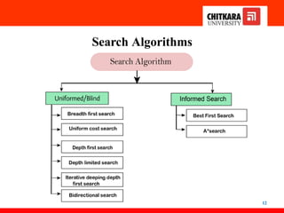
Search Algorithm
Terminologies
5
Problem-solving agents:
InArtificial Intelligence, Search techniques are universal
problem-solving methods. Rational agents or Problem-solving
agents in AI mostly used these search strategies or algorithms to
solve a specific problem and provide the best result.
Problem-solving agents are goal-based agents and use atomic
representation. A search problem consists of a search space,
start state, and goal state.
6.
Search Algorithm
Terminologies
6
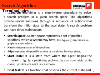
1.Search: Searchingis a step-by-step procedure to solve
a search problem in a given search space. The algorithms
provide search solutions through a sequence of actions that
transform the initial state to the goal state. A search problem
can have three main factors:
• Search Space: Search space represents a set of possible
solutions, which a system may have. It is typically structured as a
graph or a tree, where:
• Nodes represent states of the problem.
• Edges represent the possible actions or transitions between states.
• Start State: It is a state from where the agent begins the
search. Eg: In a pathfinding problem, the start state might be the
current position of a robot in a warehouse.
• Goal test: It is a function that observes the current state and
7.
Search Algorithm Terminologies
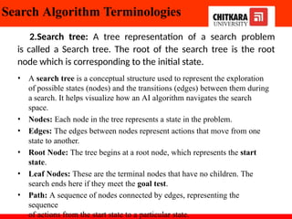
2.Searchtree: A tree representation of a search problem
is called a Search tree. The root of the search tree is the root
node which is corresponding to the initial state.
• A search tree is a conceptual structure used to represent the exploration
of possible states (nodes) and the transitions (edges) between them during
a search. It helps visualize how an AI algorithm navigates the search
space.
• Nodes: Each node in the tree represents a state in the problem.
• Edges: The edges between nodes represent actions that move from one
state to another.
• Root Node: The tree begins at a root node, which represents the start
state.
• Leaf Nodes: These are the terminal nodes that have no children. The
search ends here if they meet the goal test.
• Path: A sequence of nodes connected by edges, representing the
sequence
of actions from the start state to a particular state.
8.
• Actions definethe allowable changes in state and drive the
exploration of the search space.
• Applicability: Not all actions are applicable in every state. For
instance, in a maze, you can't move up if there's a wall above.
• Cost: Actions can have different costs, and these are considered in
algorithms like Uniform-Cost Search or A* to find optimal
solutions. Some problems involve minimizing these action costs.
Example:
• In a robot navigation problem, actions might include moving
forward, turning left, or turning right. In a game like chess, actions
would be individual moves of pieces.
Faculty Name - GroupNo 8
9.
Search Algorithm
Terminologies
node tothe goal node.
9
4. Transition model: A description of what each action does, can
be represented as a transition model.
•Egchess) Search Tree: The root node is the current
state of the chessboard. Each child node represents the
state after one legal move. The tree grows as players
explore further moves.
•Actions: Legal chess moves, such as moving a pawn
or castling.
•Transition Model: Rules of chess that define how
each piece moves (e.g., a knight moves in an L-shape,
a pawn can move forward one square).
5.Path Cost: It is a function that assigns a numeric cost to
each path.
6. Solution: It is an action sequence that leads from the start
10.
Properties For Search
Algorithms
10
Completeness:A search algorithm is said to be complete if it
guarantees to return a solution if at least any solution exists for
any random input.
Optimality: If a solution found for an algorithm is guaranteed to
be the best solution (lowest path cost) among all other solutions,
then such a solution for is said to be an optimal solution.
Time Complexity: Time complexity is a measure of time for an
algorithm to complete its task.
Space Complexity: It is the maximum storage space required at
any point during the search, as the complexity of the problem.
11.
Completeness and Optimality
FacultyName - GroupNo 11
• When a search algorithm has the property of
optimality, it means it is guaranteed to find the
best possible solution. When a search
algorithm has the property of completeness, it
means that if a solution to a given problem
exists, the algorithm is guaranteed to find it.
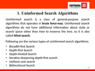
1. Uninformed SearchAlgorithms
13
Uninformed search is a class of general-purpose search
algorithms that operates in brute force-way. Uninformed search
algorithms do not have additional information about state or
search space other than how to traverse the tree, so it is also
called blind search.
Following are the various types of uninformed search algorithms:
• Breadth-first Search
• Depth-first Search
• Depth-limited Search
• Iterative deepening depth-first search
• Uniform cost search
• Bidirectional Search
14.
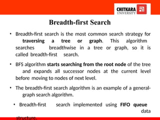
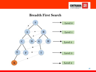
Breadth-first Search
• Breadth-firstsearch is the most common search strategy for
traversing a tree or graph. This algorithm
searches breadthwise in a tree or graph, so it is
called breadth-first search.
• BFS algorithm starts searching from the root node of the tree
and expands all successor nodes at the current level
before moving to nodes of next level.
• The breadth-first search algorithm is an example of a general-
graph search algorithm.
• Breadth-first search implemented using FIFO queue
data
structure.
Breadth-first Search
16
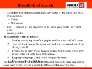
• Astandard BFS implementation puts each vertex of the graph into one of
two categories:
– Visited
– Not Visited
• The purpose of the algorithm is to mark each vertex as visited
while
avoiding cycles.
The algorithm works as follows:
1. Start by putting any one of the graph's vertices at the back of a queue.
2. Take the front item of the queue and add it to the visited list (if not
already visited).
3. Create a list of that vertex's adjacent nodes. Add the ones which aren't
in the visited list to the back of the queue.
4. Keep repeating steps 2 and 3 until the queue is empty.
5. Print visited list for BFS Traversal.
The graph might have two different disconnected parts so to make sure that we
cover every vertex, we can also run the BFS algorithm on every node
17.
Breadth-first Search Pseudocode
17
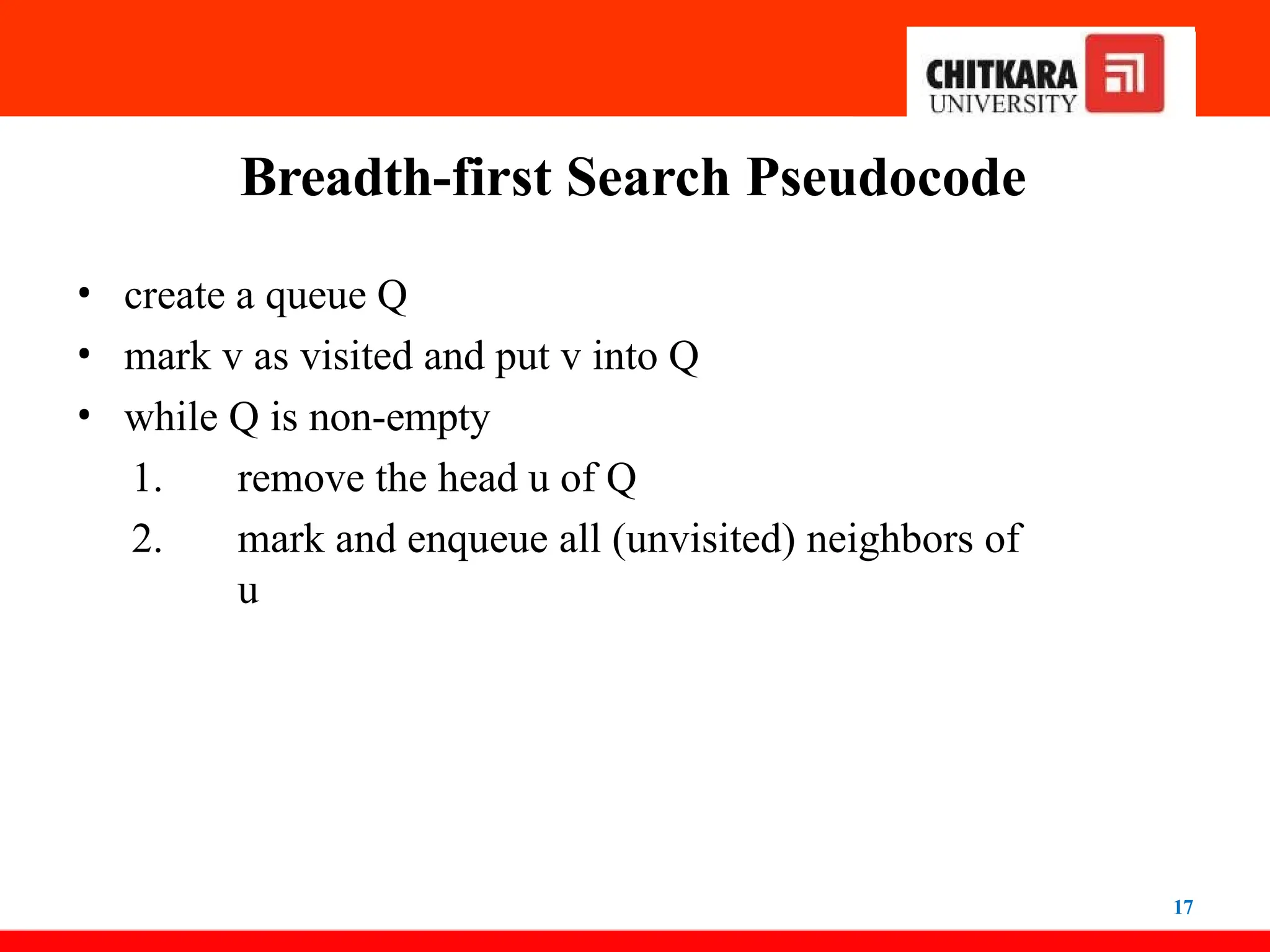
•create a queue Q
• mark v as visited and put v into Q
• while Q is non-empty
1. remove the head u of Q
2. mark and enqueue all (unvisited) neighbors of
u
18.
Breadth-first Search
18
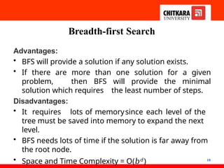
Advantages:
• BFSwill provide a solution if any solution exists.
• If there are more than one solution for a given
problem, then BFS will provide the minimal
solution which requires the least number of steps.
Disadvantages:
• It requires lots of memorysince each level of the
tree must be saved into memory to expand the next
level.
• BFS needs lots of time if the solution is far away from
the root node.
• Space and Time Complexity = O(𝑏𝑑)
19.
Real-World Problem Solvedusing BFS
Faculty Name - GroupNo 19
• Snake and Ladder Problem
• Chess Knight Problem
• Shortest path in a maze
• Flood Fill Algorithm
• Count number of islands
https://medium.com/techie-delight/top-20-breadth-first-search-bfs-
practice-problems-ac2812283ab1
20.
Depth-first Search
20
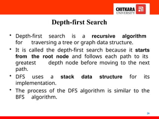
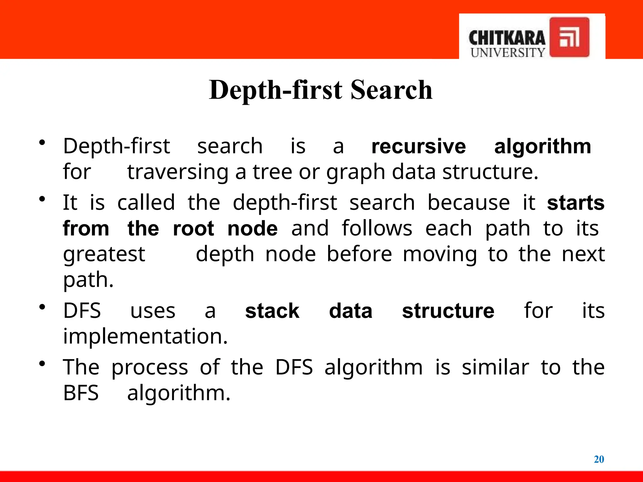
• Depth-firstsearch is a recursive algorithm
for traversing a tree or graph data structure.
• It is called the depth-first search because it starts
from the root node and follows each path to its
greatest depth node before moving to the next
path.
• DFS uses a stack data structure for its
implementation.
• The process of the DFS algorithm is similar to the
BFS algorithm.
21.
Depth-first Search
21
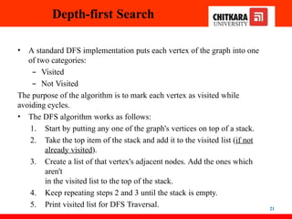
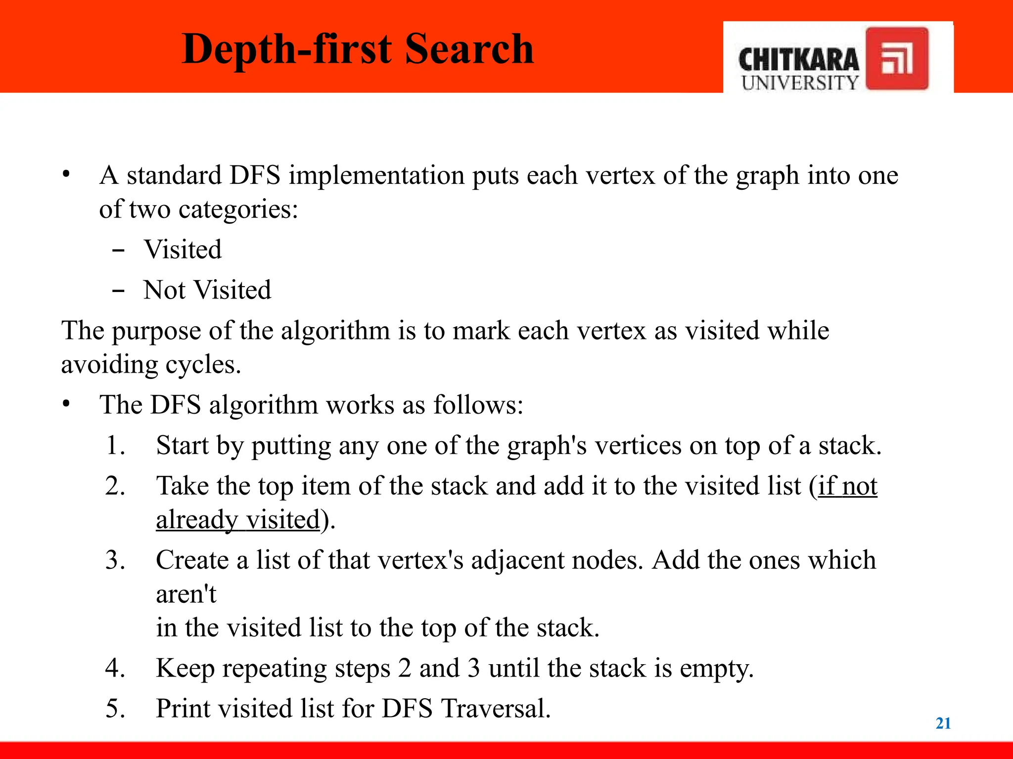
• Astandard DFS implementation puts each vertex of the graph into one
of two categories:
– Visited
– Not Visited
The purpose of the algorithm is to mark each vertex as visited while
avoiding cycles.
• The DFS algorithm works as follows:
1. Start by putting any one of the graph's vertices on top of a stack.
2. Take the top item of the stack and add it to the visited list (if not
already visited).
3. Create a list of that vertex's adjacent nodes. Add the ones which
aren't
in the visited list to the top of the stack.
4. Keep repeating steps 2 and 3 until the stack is empty.
5. Print visited list for DFS Traversal.
22.
Depth-first Search Pseudocode
22
DFS(G,u)
u.visited = true
for each v ∈
G.Adj[u]
if v.visited == false
DFS(G,v)
init() {
For each u ∈ G
u.visited = false
For each u ∈ G
DFS(G, u)
}
23.
Depth-first Search
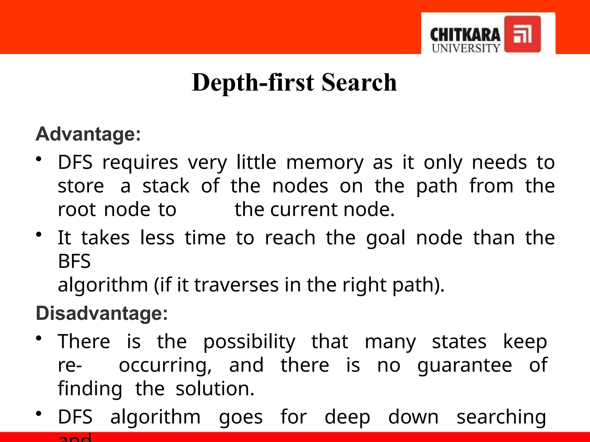
Advantage:
• DFSrequires very little memory as it only needs to
store a stack of the nodes on the path from the
root node to the current node.
• It takes less time to reach the goal node than the
BFS
algorithm (if it traverses in the right path).
Disadvantage:
• There is the possibility that many states keep
re- occurring, and there is no guarantee of
finding the solution.
• DFS algorithm goes for deep down searching
24.
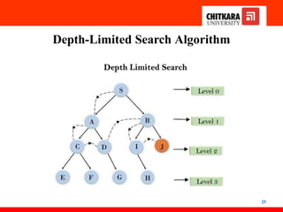
Depth-Limited Search Algorithm
24
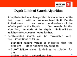
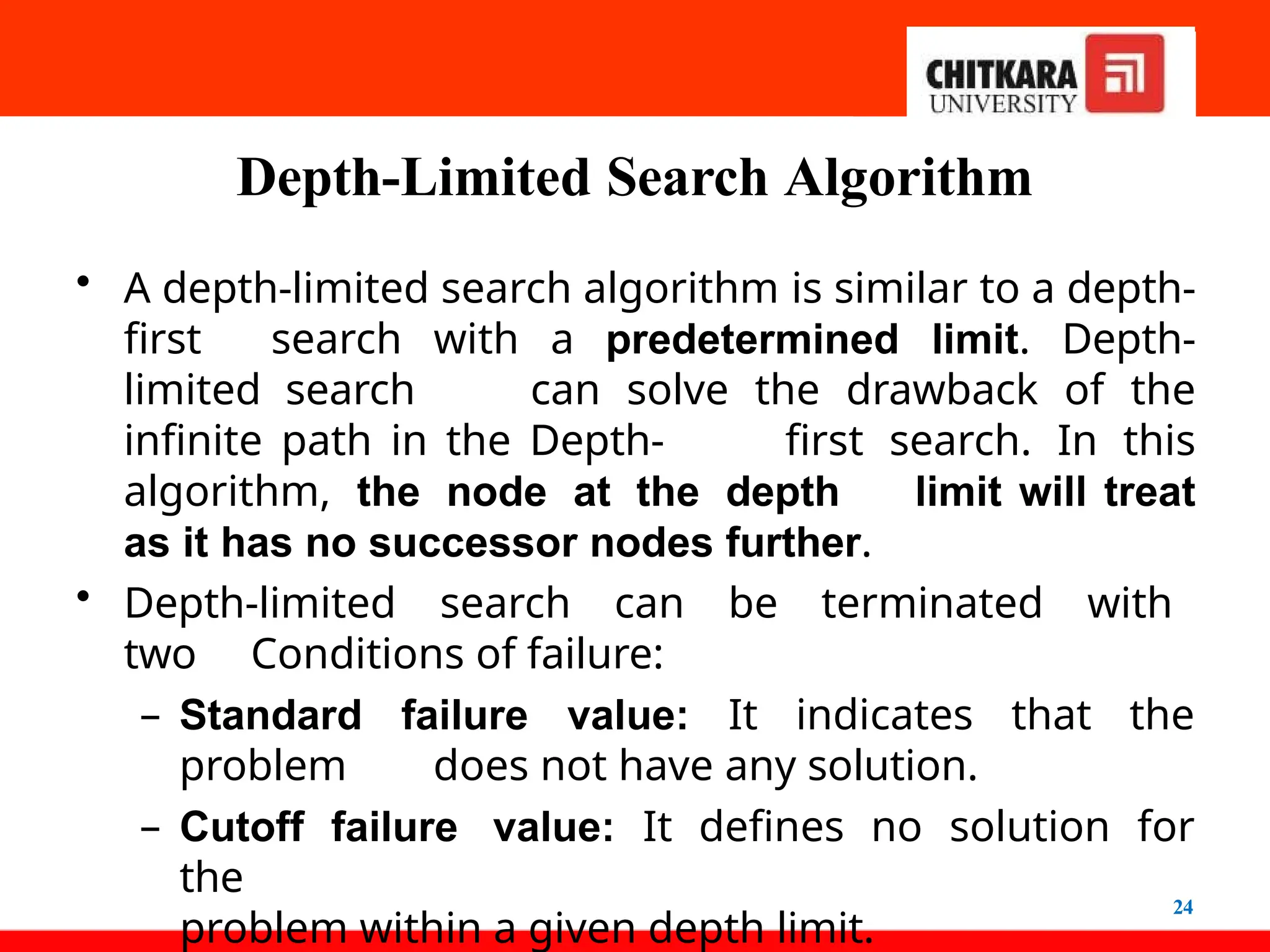
•A depth-limited search algorithm is similar to a depth-
first search with a predetermined limit. Depth-
limited search can solve the drawback of the
infinite path in the Depth- first search. In this
algorithm, the node at the depth limit will treat
as it has no successor nodes further.
• Depth-limited search can be terminated with
two Conditions of failure:
– Standard failure value: It indicates that the
problem does not have any solution.
– Cutoff failure value: It defines no solution for
the
problem within a given depth limit.
Depth-Limited Search Algorithm
26
Advantages:
•Depth-limited search is Memory efficient.
Disadvantages:
• Depth-limited search also has
a incompleteness.
disadvantage of
• It may not be optimal if the problem has more than
one solution.
27.
Uniform-Cost Search Algorithm
•Uniform-cost search is a searching algorithm used
for traversing a weighted tree or graph. This
algorithm comes into play when a different cost
is available for each edge.
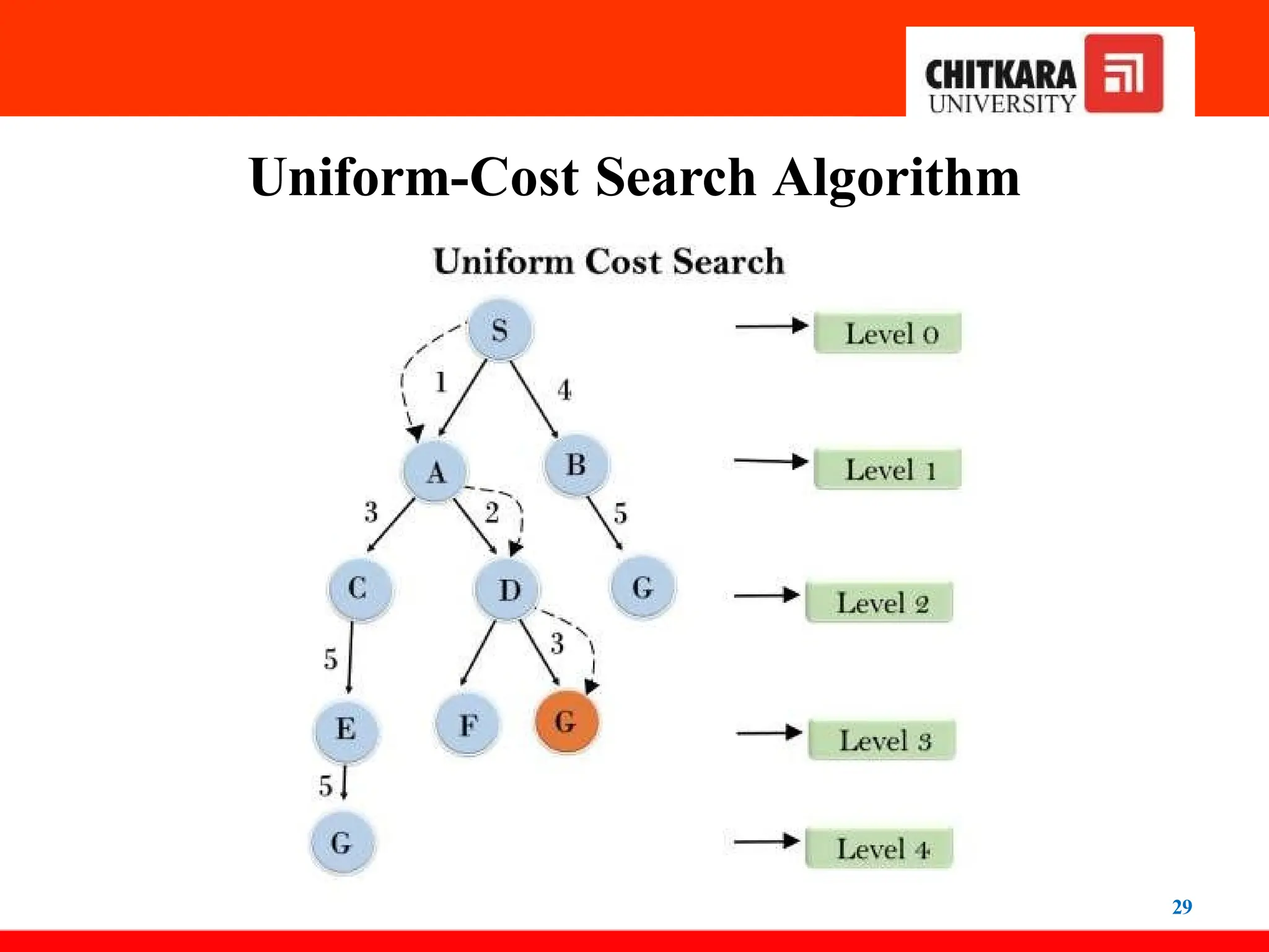
• The primary goal of the uniform-cost search is to
find a path to the goal node which has the lowest
cumulative cost. Uniform-cost search expands
nodes according to their path costs from the
root node.
• It can be used to solve any graph/tree where the
optimal cost is in demand. A uniform-cost
search algorithm is implemented by the
priority queue. It gives maximum priority to the
28.
Uniform-Cost Search Algorithm
28
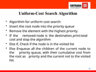
•Algorithm for uniform cost search:
• Insert the root node into the priority queue
• Remove the element with the highest priority.
• If the removed node is the destination,print total
cost and stop the algorithm
• Else if, Check if the node is in the visited list
• Else Enqueue all the children of the current node to
the priority queue, with their cumulative cost from
the root as priority and the current not to the visited
list.
Uniform-Cost Search Algorithm
30
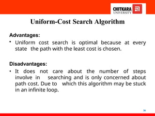
Advantages:
•Uniform cost search is optimal because at every
state the path with the least cost is chosen.
Disadvantages:
• It does not care about the number of steps
involve in searching and is only concerned about
path cost. Due to which this algorithm may be stuck
in an infinite loop.
31.
Iterative deepening depth-firstSearch
31
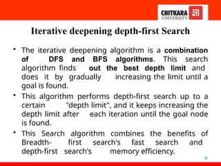
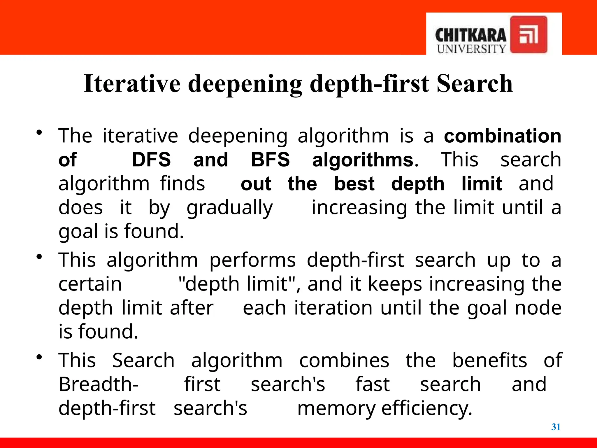
• The iterative deepening algorithm is a combination
of DFS and BFS algorithms. This search
algorithm finds out the best depth limit and
does it by gradually increasing the limit until a
goal is found.
• This algorithm performs depth-first search up to a
certain "depth limit", and it keeps increasing the
depth limit after each iteration until the goal node
is found.
• This Search algorithm combines the benefits of
Breadth- first search's fast search and
depth-first search's memory efficiency.
32.
Iterative deepening depth-firstSearch
32
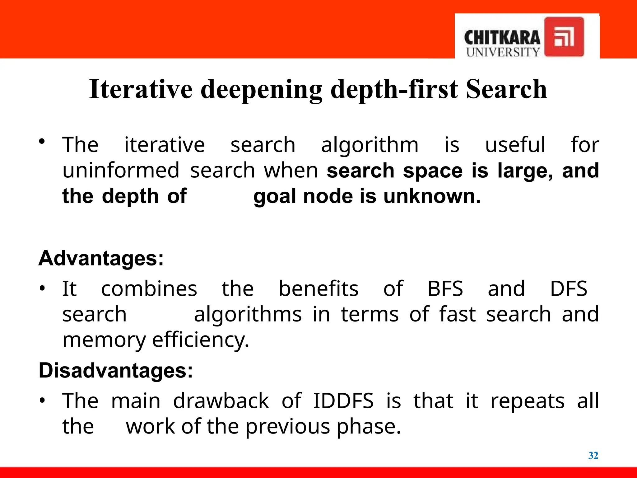
• The iterative search algorithm is useful for
uninformed search when search space is large, and
the depth of goal node is unknown.
Advantages:
• It combines the benefits of BFS and DFS
search algorithms in terms of fast search and
memory efficiency.
Disadvantages:
• The main drawback of IDDFS is that it repeats all
the work of the previous phase.
33.
Iterative deepening depth-firstSearch
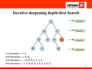
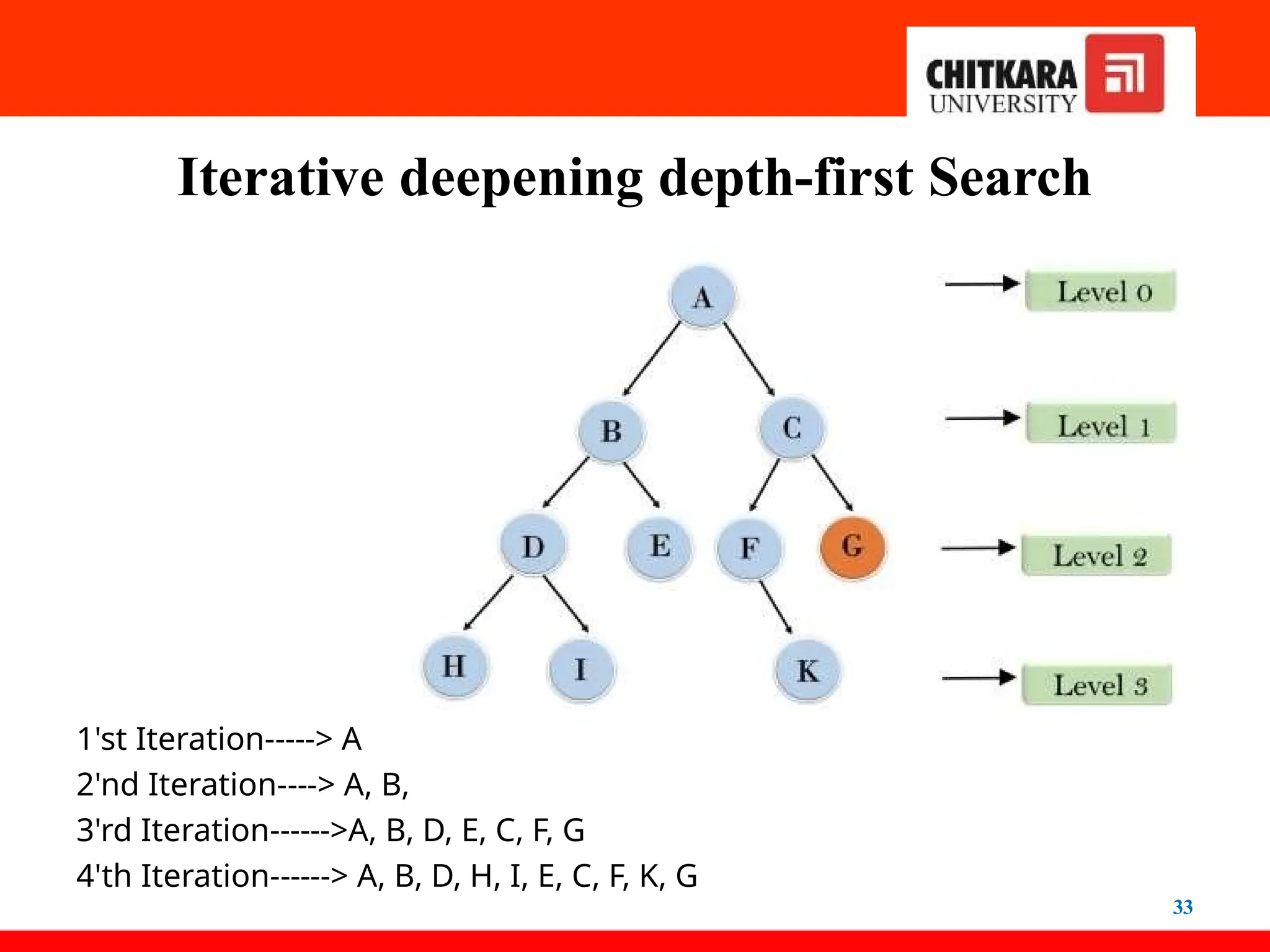
1'st Iteration-----> A
2'nd Iteration----> A, B, C
3'rd Iteration------>A, B, D, E, C, F, G
4'th Iteration------> A, B, D, H, I, E, C, F, K, G
33
34.
Bidirectional Search Algorithm
34
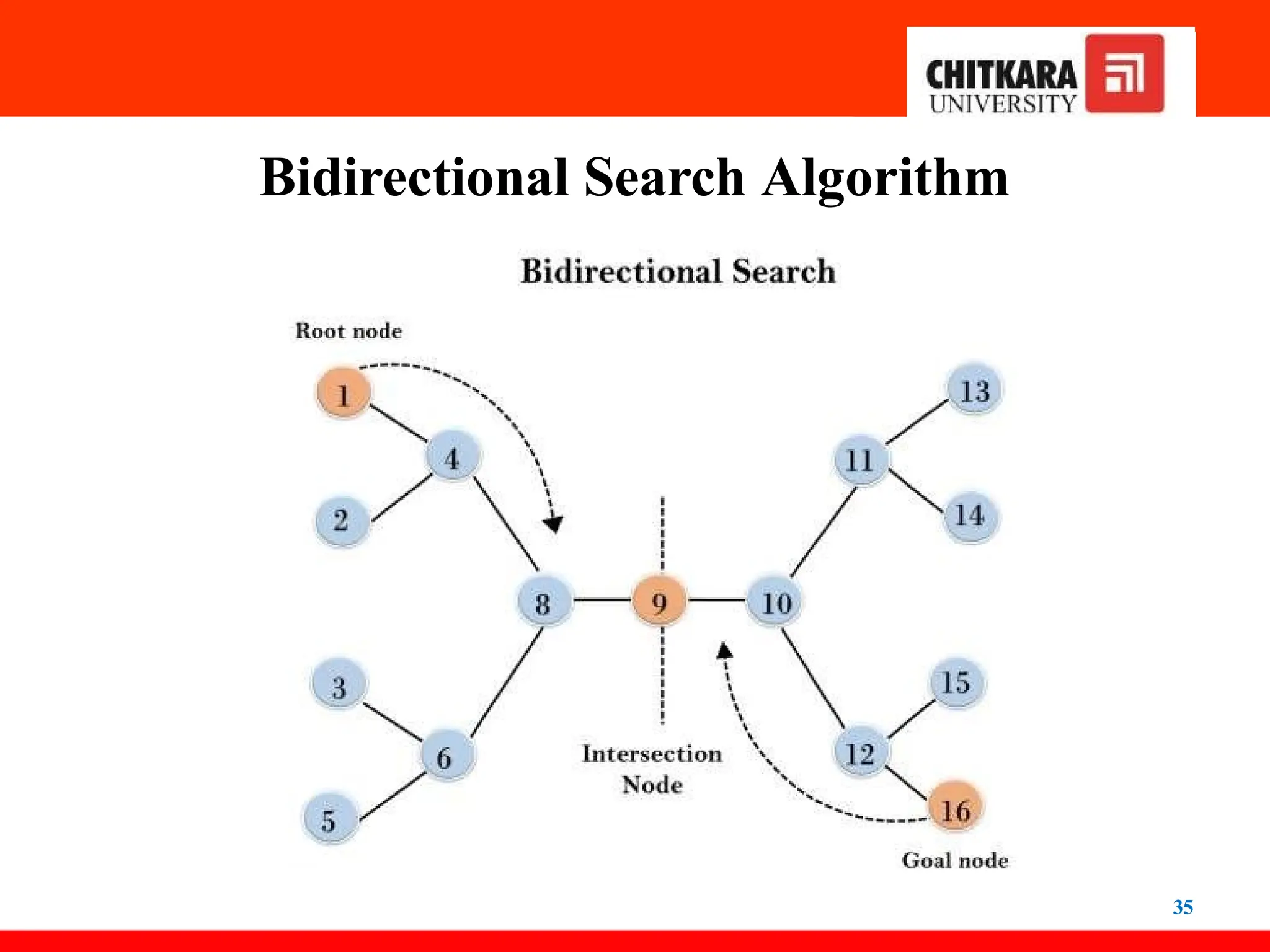
•Bidirectional search algorithm runs two simultaneous
searches, one from the initial state called forward-search
and the other from the goal node called backward-search,
to find the goal node.
• Bidirectional search replaces one single search graph with two
small subgraphs in which one starts the search from an
initial vertex and the other starts from the goal vertex.
• The search stops when these two graphs intersect each
other.
• Bidirectional search can use search techniques such as BFS,
DFS, etc.
Bidirectional Search Algorithm
36
Advantages:
•Bidirectional search is fast.
• Bidirectional search requires less memory
Disadvantages:
• Implementation of the bidirectional search tree is difficult.
• In bidirectional search, one should know the goal state
in
advance.
37.
2. Informed SearchAlgorithms
37
• The informed search algorithm is more useful for large search
spaces. An informed search algorithm uses the idea
of heuristic, so it is also called Heuristic search.
• Heuristics function: Heuristic is a function that is used in
Informed Search, and it finds the most promising path. It
takes the current state of the agent as its input and
produces the estimation of how close the agent is to the goal.
• Heuristic function estimates how close a state is to the goal.
• The heuristic method, however, might not always give the best
solution, but it guarantees to find a good solution in
a reasonable time.
38.
2. Informed SearchAlgorithms
38
• A heuristic function helps the search algorithm choose a branch
from the ones that are available. It helps with the
decision process by using some extra knowledge about
the search space.
• Let’s use a simple analogy. If you went to a supermarket with
many check-out counters, you would try to go to the one
with the least number of people waiting. This is a
heuristic that reduces your wait time.
39.
2. Informed SearchAlgorithms
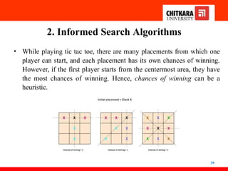
• While playing tic tac toe, there are many placements from which one
player can start, and each placement has its own chances of winning.
However, if the first player starts from the centermost area, they have
the most chances of winning. Hence, chances of winning can be a
heuristic.
39
40.
2. Informed SearchAlgorithms
40
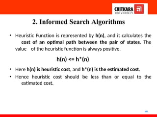
• Heuristic Function is represented by h(n), and it calculates the
cost of an optimal path between the pair of states. The
value of the heuristic function is always positive.
h(n) <= h*(n)
• Here h(n) is heuristic cost, and h*(n) is the estimated cost.
• Hence heuristic cost should be less than or equal to the
estimated cost.
41.
2. Informed SearchAlgorithms
41
Pure Heuristic Search:
• Pure heuristic search is the simplest form of heuristic search
algorithms. It expands nodes based on their heuristic
value
h(n). It maintains two lists, OPEN and CLOSED lists. In the
CLOSED list, it places those nodes which have already
expanded, and in the OPEN list, it places nodes that have yet
not been expanded.
• On each iteration, each node n with the lowest heuristic value
is expanded and generates all its successors, and n is placed
to the closed list. The algorithm continues unit a goal state
is found.
42.
2. Informed SearchAlgorithms
42
In the informed search we will discuss two main algorithms which
are given below:
1. Best First Search Algorithm (Greedy search)
2. A* Search Algorithm
43.
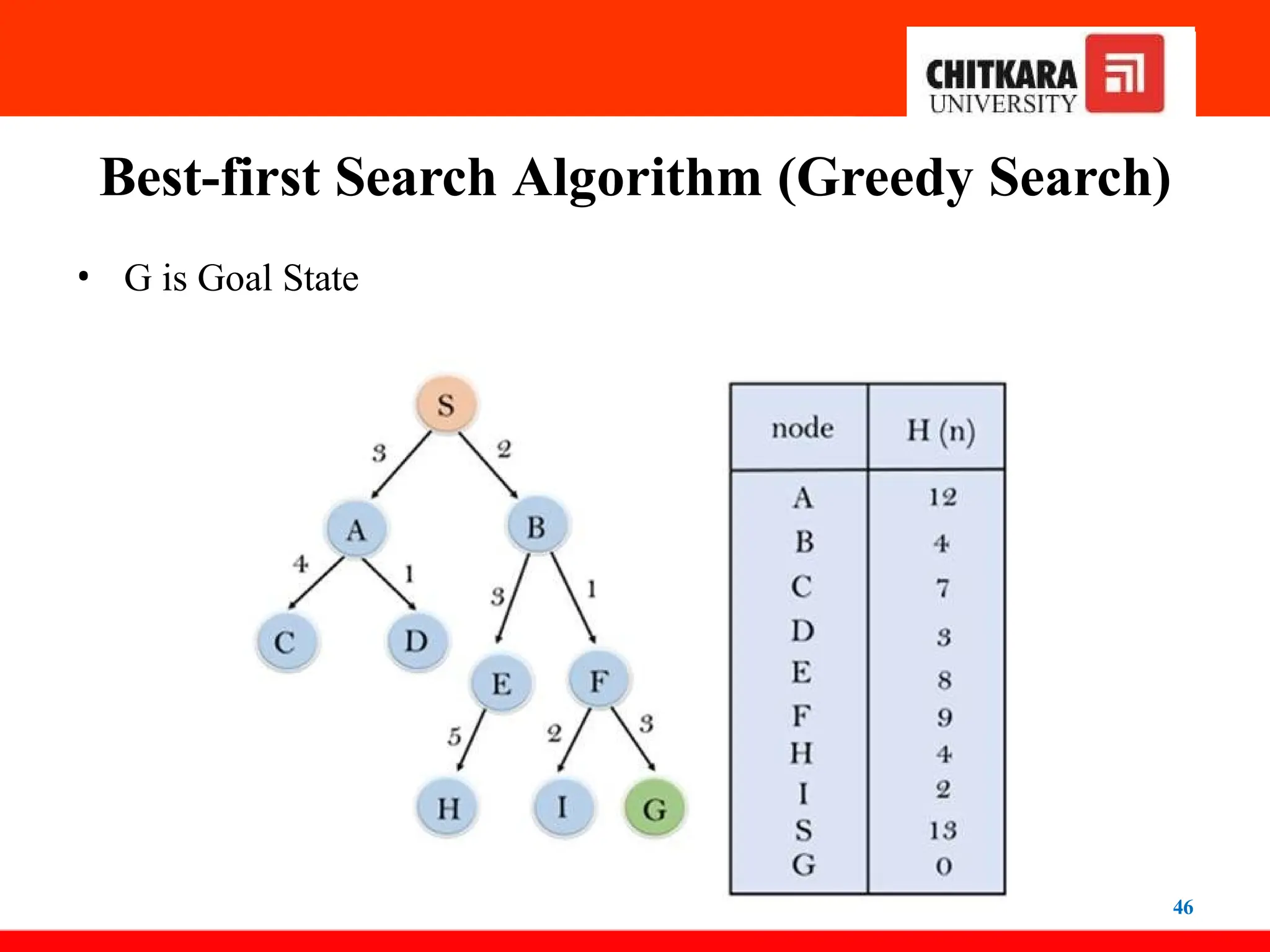
Best-first Search Algorithm(Greedy Search)
43
• Greedy best-first search algorithm always selects the path
which appears best at that moment. It is the combination
of depth-first search and breadth-first search algorithms.
• It uses the heuristic function and search. Best-first search allows
us to take advantage of both algorithms. With the help of
the best-first search, at each step, we can choose
the most promising node. The greedy best-first algorithm
is implemented by the priority queue.
• In the best-first search algorithm, we expand the node which is
closest to the goal node, and the closest cost is estimated
by heuristic function, i.e.
44.
Best-first Search Algorithm(Greedy Search)
44
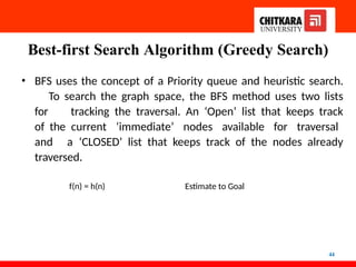
• BFS uses the concept of a Priority queue and heuristic search.
To search the graph space, the BFS method uses two lists
for tracking the traversal. An ‘Open’ list that keeps track
of the current ‘immediate’ nodes available for traversal
and a ‘CLOSED’ list that keeps track of the nodes already
traversed.
f(n) = h(n) Estimate to Goal
45.
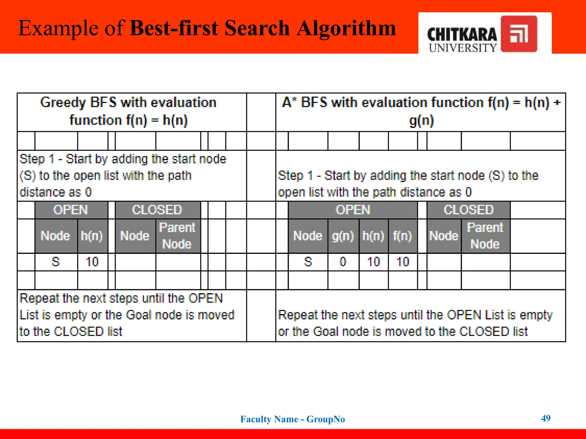
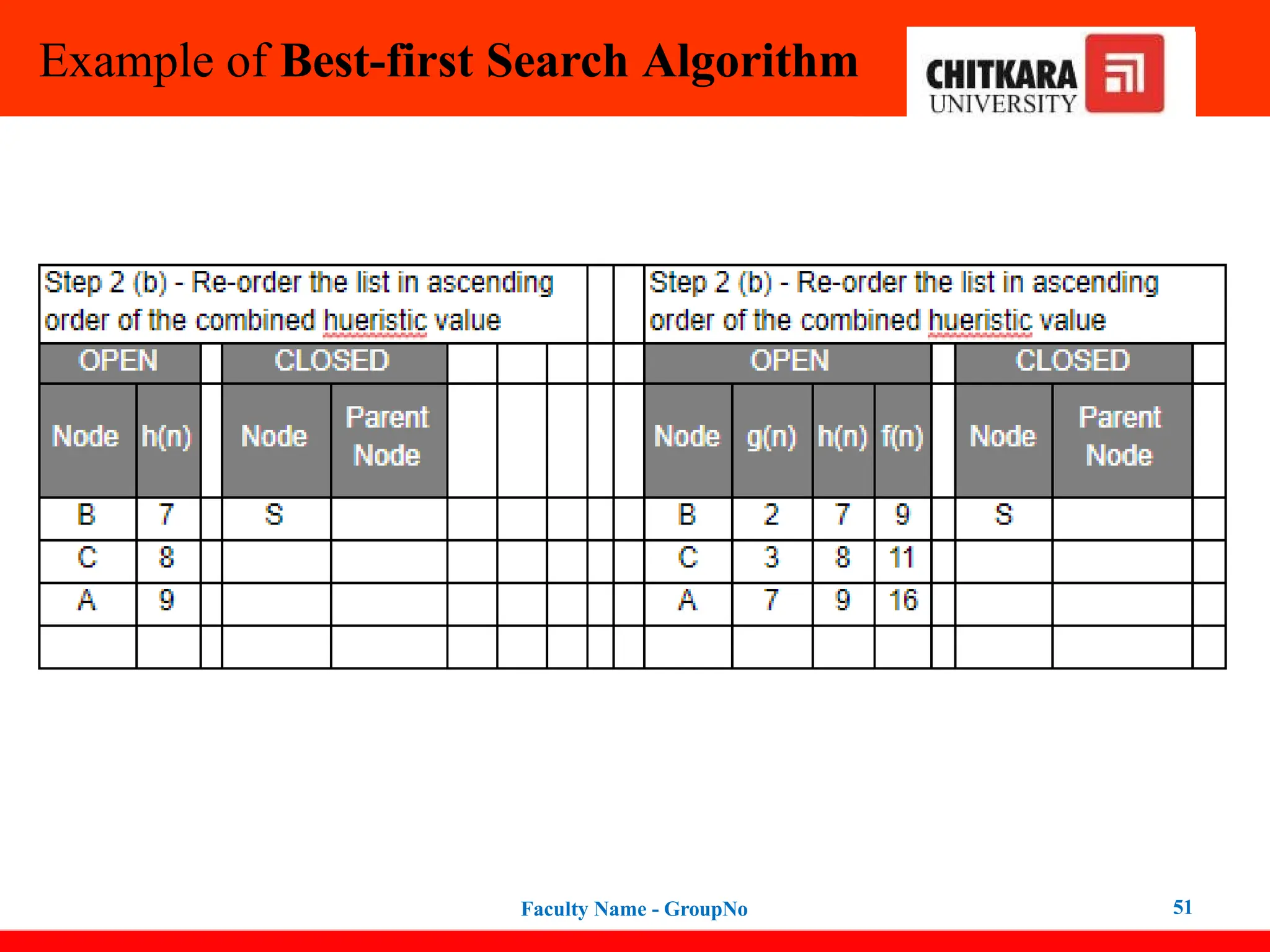
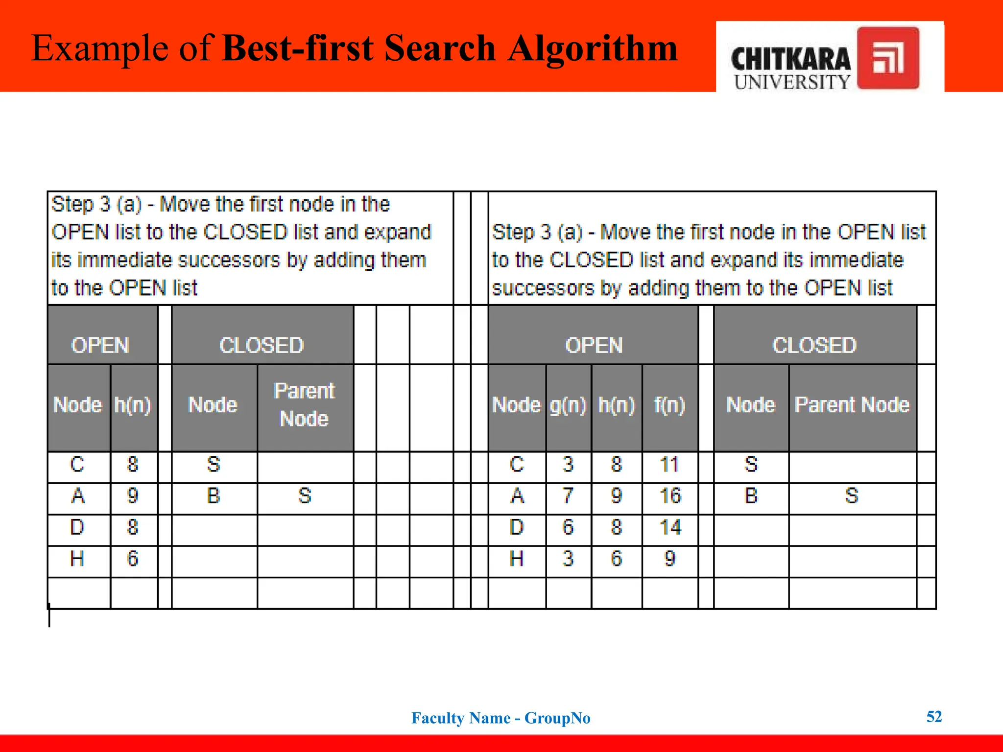
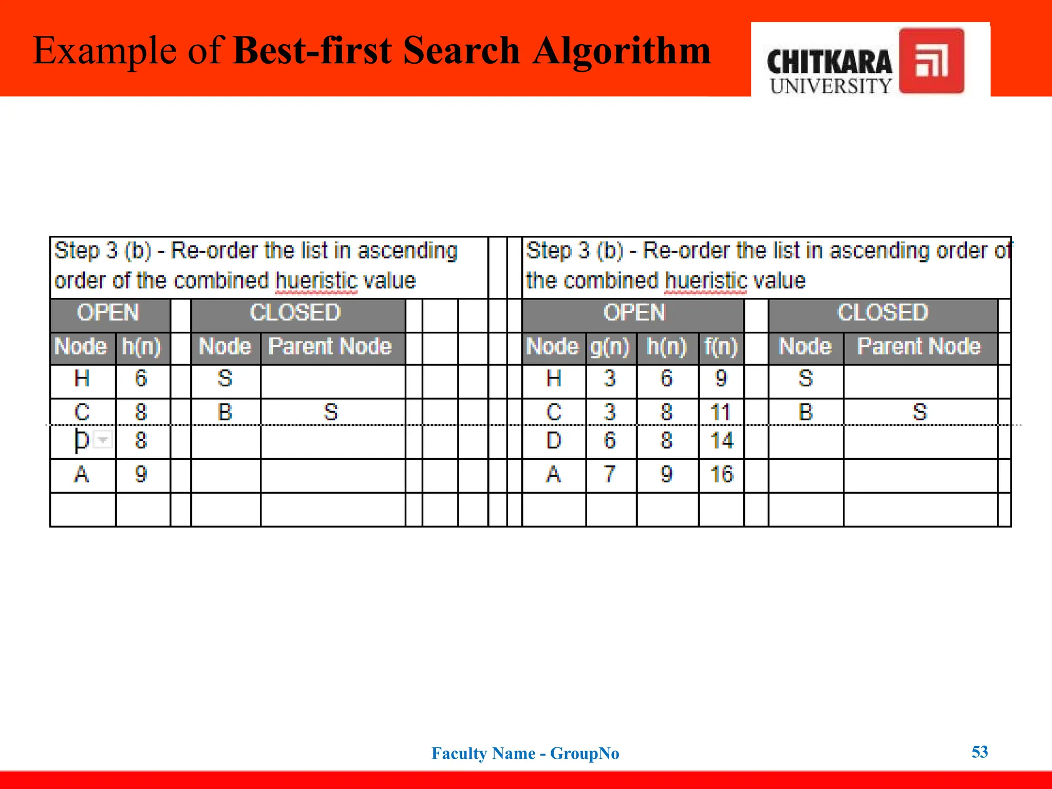
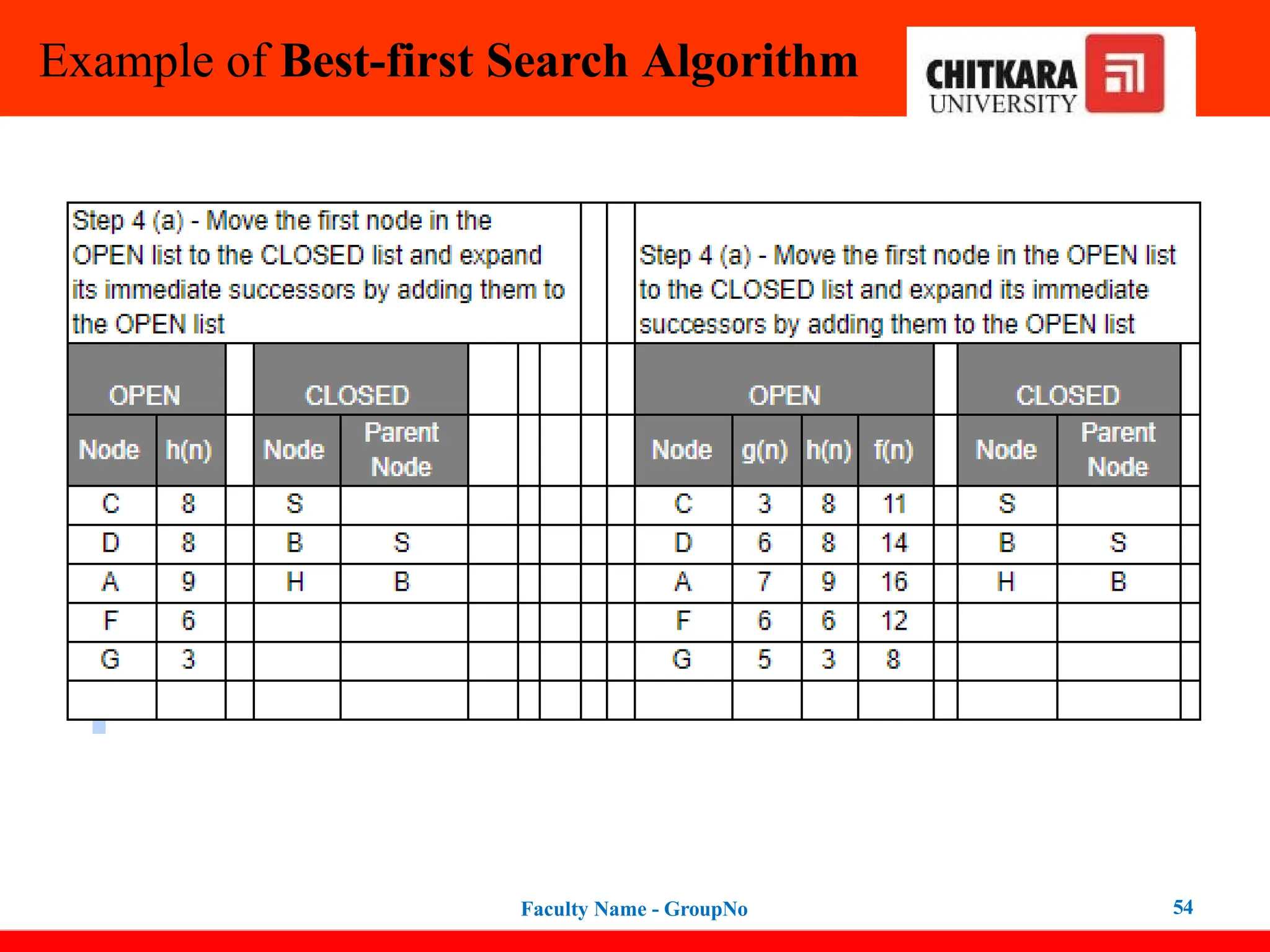
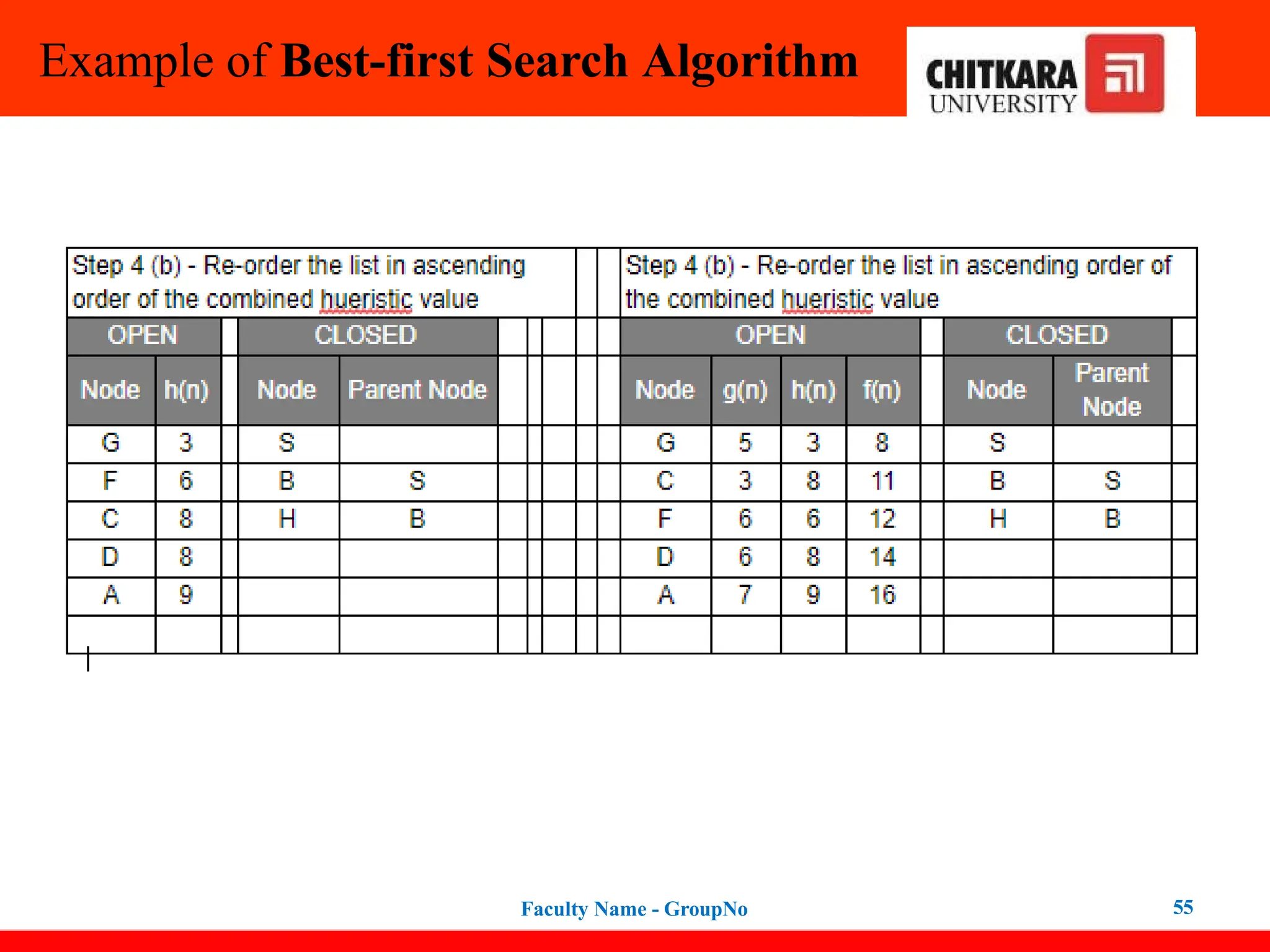
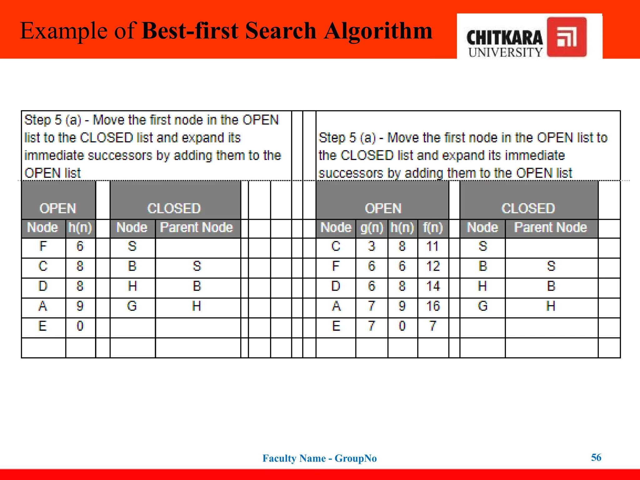
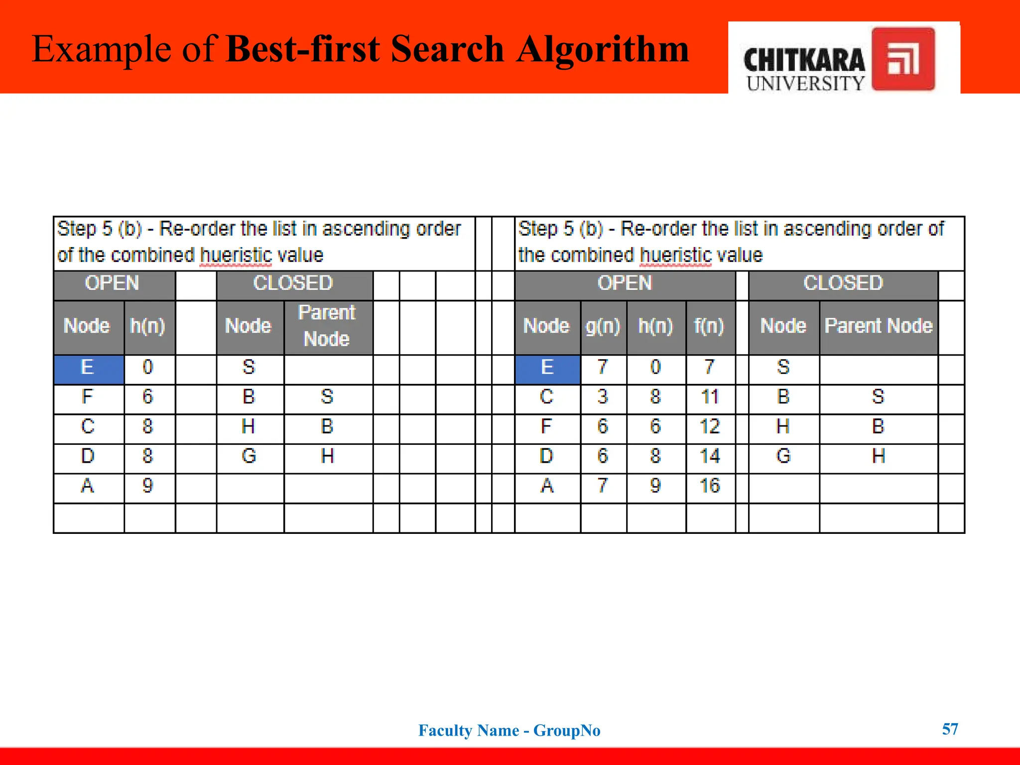
Best-first Search Algorithm(Greedy Search)
45
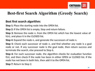
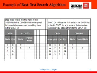
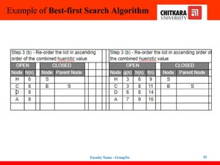
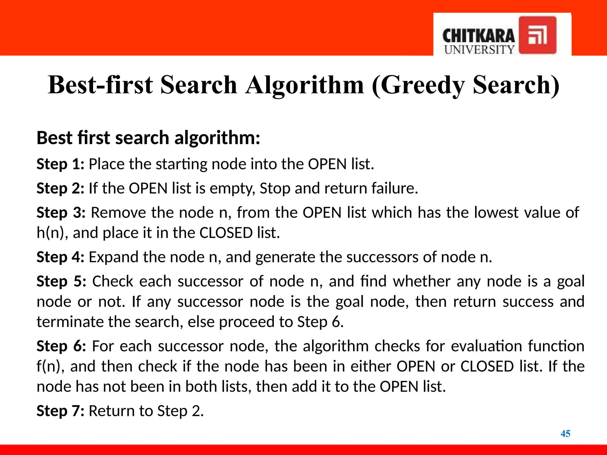
Best first search algorithm:
Step 1: Place the starting node into the OPEN list.
Step 2: If the OPEN list is empty, Stop and return failure.
Step 3: Remove the node n, from the OPEN list which has the lowest value of
h(n), and place it in the CLOSED list.
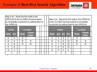
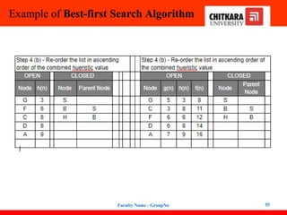
Step 4: Expand the node n, and generate the successors of node n.
Step 5: Check each successor of node n, and find whether any node is a goal
node or not. If any successor node is the goal node, then return success and
terminate the search, else proceed to Step 6.
Step 6: For each successor node, the algorithm checks for evaluation function
f(n), and then check if the node has been in either OPEN or CLOSED list. If the
node has not been in both lists, then add it to the OPEN list.
Step 7: Return to Step 2.
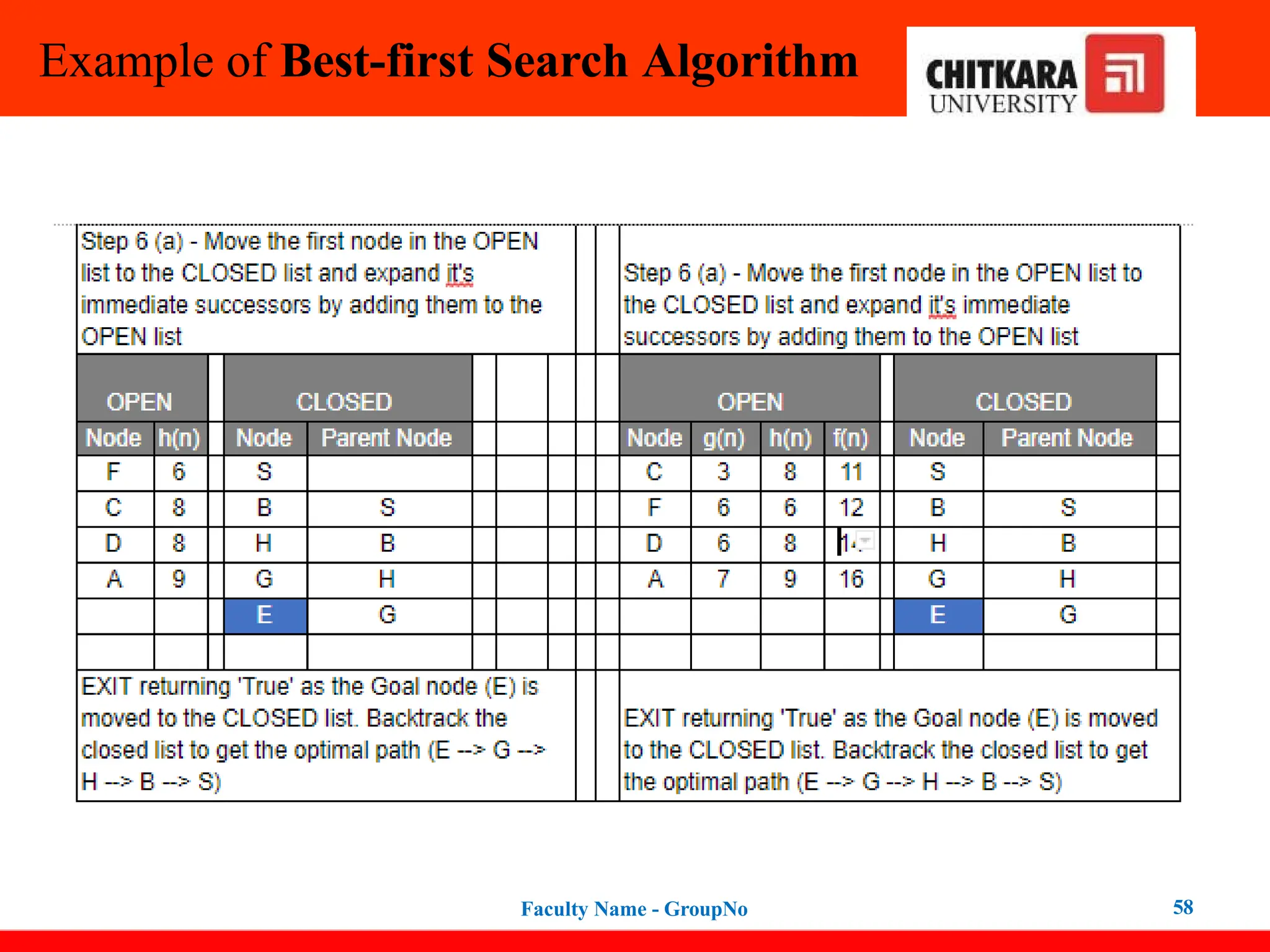
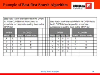
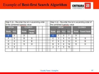
Best-first Search Algorithm(Greedy Search)
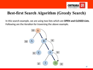
In this search example, we are using two lists which are OPEN and CLOSED Lists.
Following are the iteration for traversing the above example.
47
48.
Best-first Search Algorithm(Greedy Search)
48
Expand the nodes of S and put in the CLOSED list
Initialization: Open [B, A], Closed [S]
Iteration 1: Open [A], Closed [S, B]
Iteration 2: Open [E, F, A], Closed [S, B]
: Open [F, A], Closed [S, B, E]
Iteration 3: Open [F, A], Closed [S, B, E]
: Open [A], Closed [S, B, E, F]
Iteration 4: Open [G, I, A], Closed [S, B,
E, F]
: Open [I, A], Closed [S, B, E,
F, G]
Hence the final solution path will be:
S----> B----->F----> G
Best-first Search Algorithm(Greedy Search)
59
f(n)= g(n)
Were, g(n)= estimated cost from node n to the goal.
Advantages:
• Best first search can switch between BFS and DFS by gaining the
advantages of both the algorithms.
• This algorithm is more efficient than BFS and DFS algorithms.
Disadvantages:
• It can behave as an unguided depth-first search in the worst-
case scenario.
• It can get stuck in a loop as DFS.
• This algorithm is not optimal.
60.
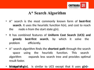
A* Search Algorithm
60
•A* search is the most commonly known form of best-first
search. It uses the heuristic function h(n), and cost to reach
the node n from the start state g(n).
• It has combined features of Uniform Cost Search (UCS) and
greedy best-first search, by which it solve the
problem efficiently.
• A* search algorithm finds the shortest path through the search
space using the heuristic function. This search
algorithm expands less search tree and provides optimal
result faster.
• A*algorithm is similar to UCS except that it uses g(n)
instead of g(n).
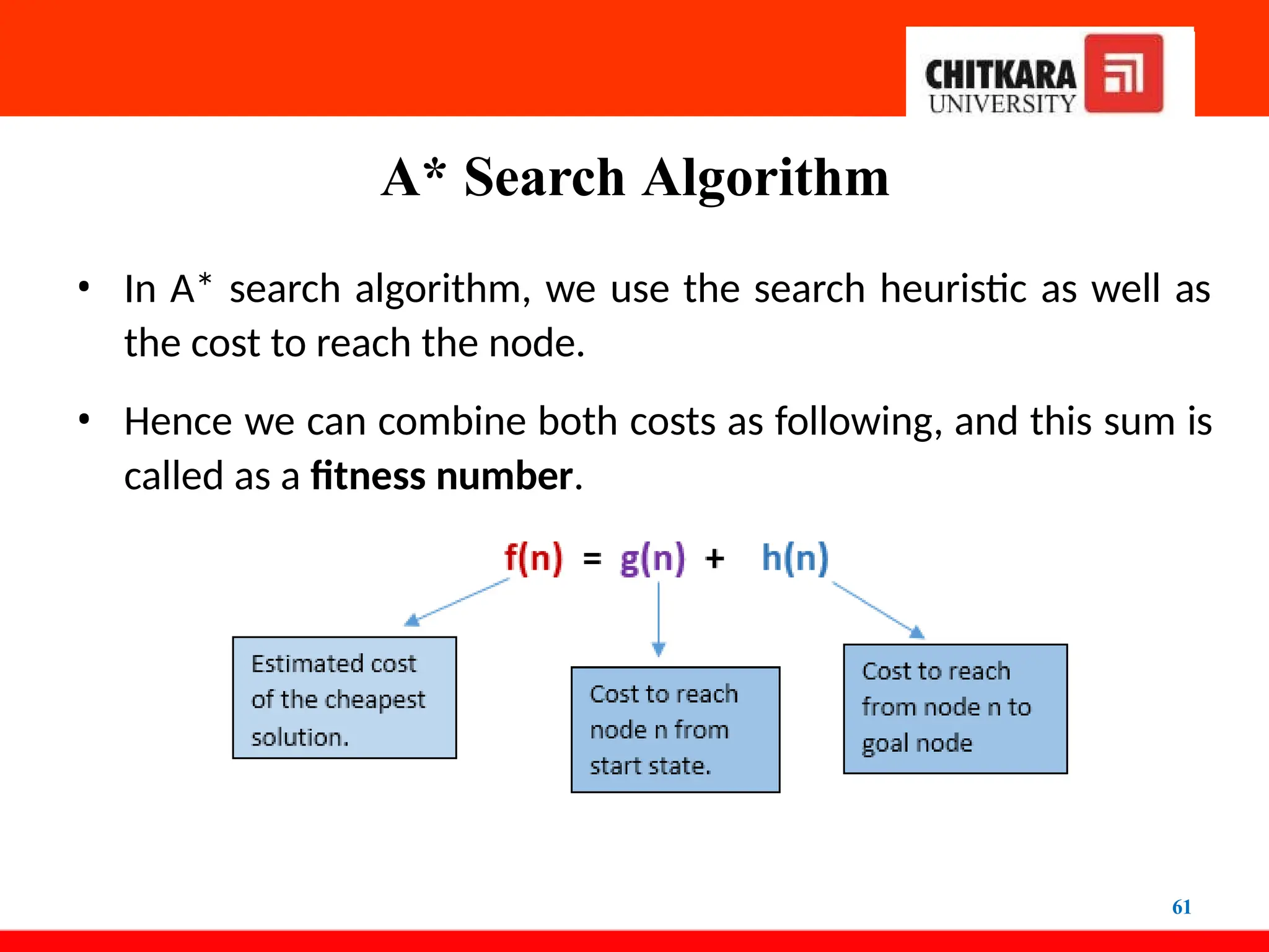
61.
A* Search Algorithm
61
•In A* search algorithm, we use the search heuristic as well as
the cost to reach the node.
• Hence we can combine both costs as following, and this sum is
called as a fitness number.
62.
A* Search Algorithm
62
Algorithmof A* search:
Step1: Place the starting node in the OPEN list.
Step 2: Check if the OPEN list is empty or not, if the list is empty
then return failure and stops.
Step 3: Select the node from the OPEN list which has the smallest
value of evaluation function (g+h), if node n is goal node then
return success and stop, otherwise
Step 4: Expand node n and generate all of its successors, and put n
into the closed list. For each successor n', check whether n' is
already in the OPEN or CLOSED list, if not then compute evaluation
function for n' and place into the Open list.
63.
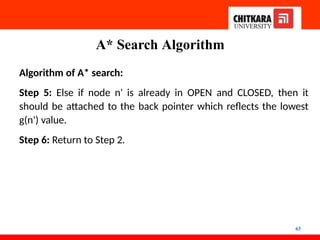
A* Search Algorithm
63
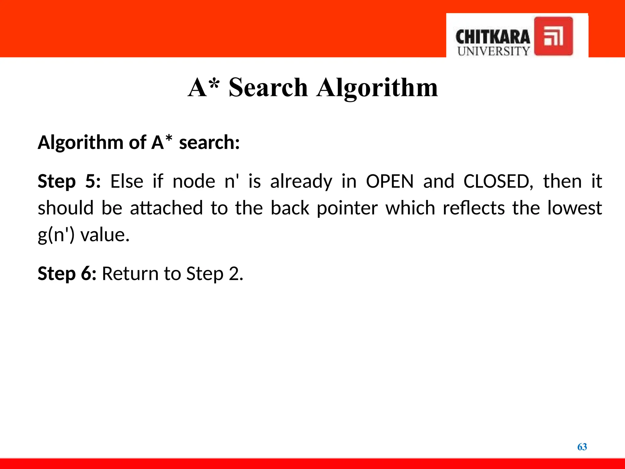
Algorithmof A* search:
Step 5: Else if node n' is already in OPEN and CLOSED, then it
should be attached to the back pointer which reflects the lowest
g(n') value.
Step 6: Return to Step 2.
64.
A* Search Algorithm
64
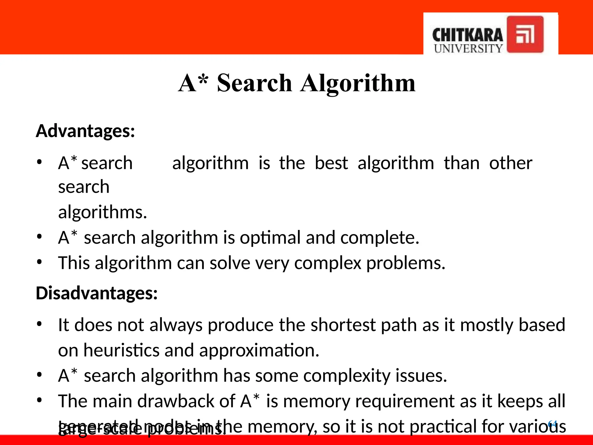
Advantages:
•A*search algorithm is the best algorithm than other
search
algorithms.
• A* search algorithm is optimal and complete.
• This algorithm can solve very complex problems.
Disadvantages:
• It does not always produce the shortest path as it mostly based
on heuristics and approximation.
• A* search algorithm has some complexity issues.
• The main drawback of A* is memory requirement as it keeps all
generated nodes in the memory, so it is not practical for various
large-scale problems.
A* Search Algorithm
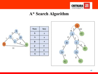
66
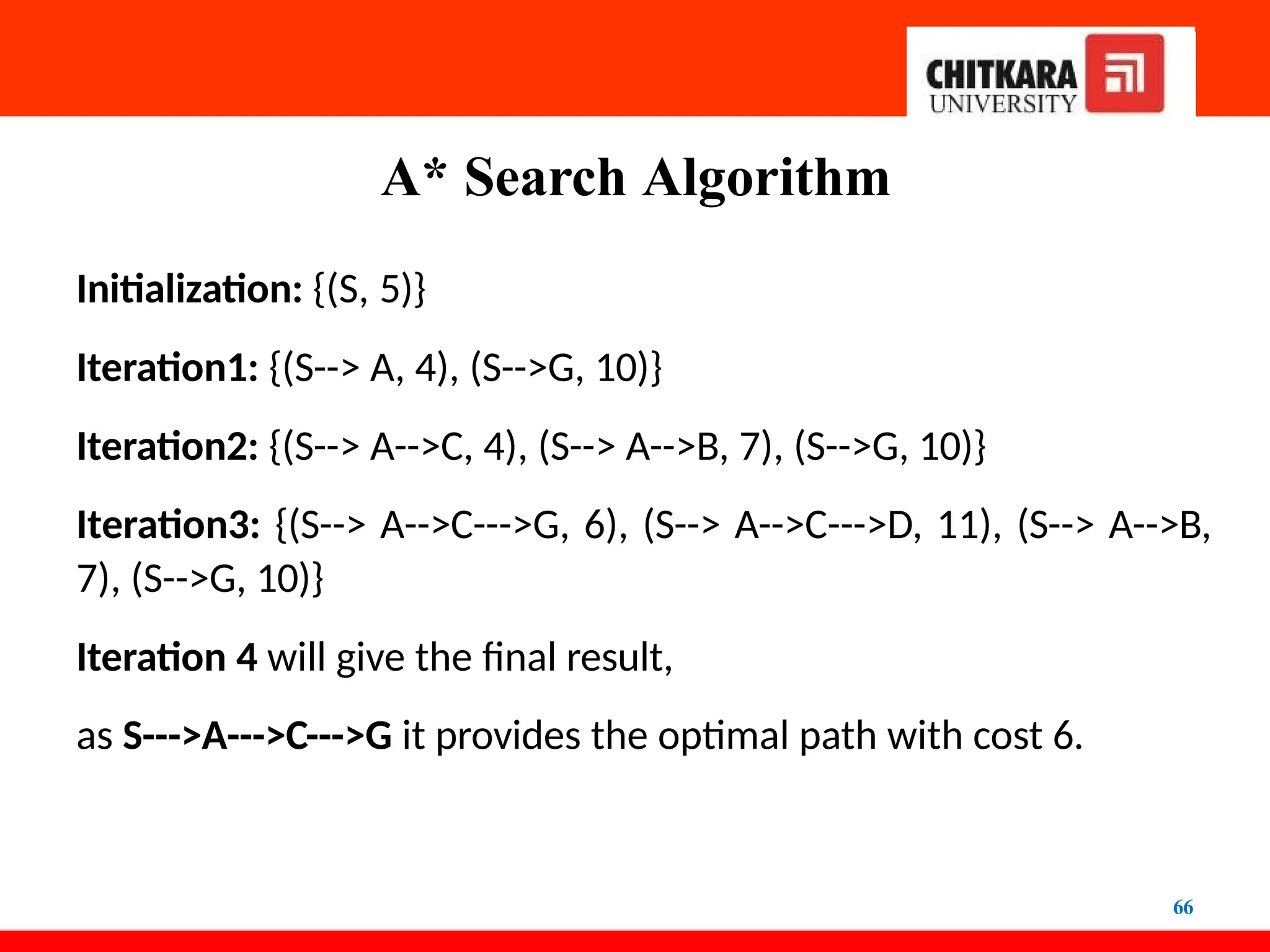
Initialization:{(S, 5)}
Iteration1: {(S--> A, 4), (S-->G, 10)}
Iteration2: {(S--> A-->C, 4), (S--> A-->B, 7), (S-->G, 10)}
Iteration3: {(S--> A-->C--->G, 6), (S--> A-->C--->D, 11), (S--> A-->B,
7), (S-->G, 10)}
Iteration 4 will give the final result,
as S--->A--->C--->G it provides the optimal path with cost 6.
67.
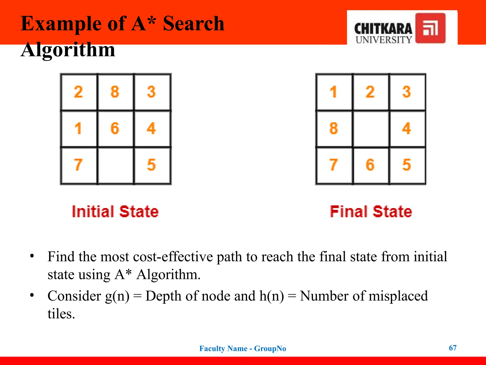
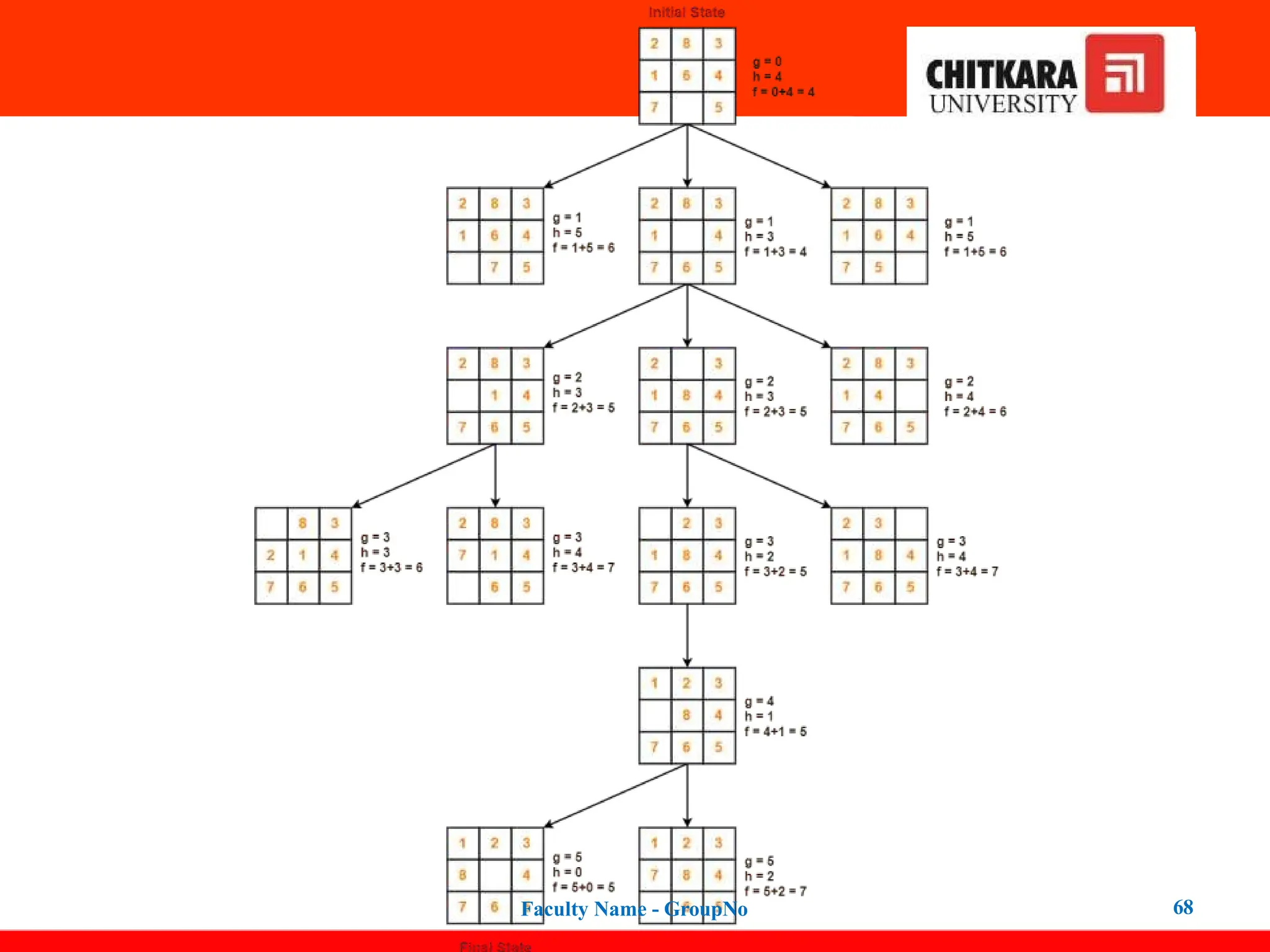
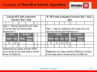
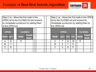
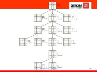
Example of A*Search
Algorithm
• Find the most cost-effective path to reach the final state from initial
state using A* Algorithm.
• Consider g(n) = Depth of node and h(n) = Number of misplaced
tiles.
Faculty Name - GroupNo 67
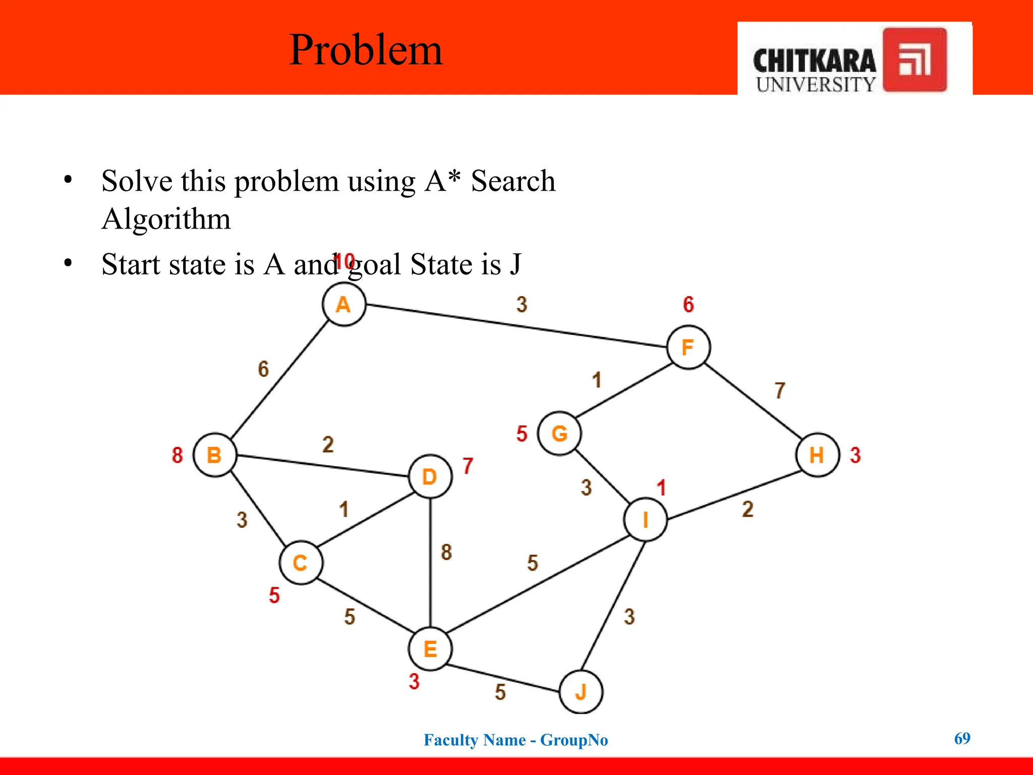
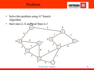
Problem
• Solve thisproblem using A* Search
Algorithm
• Start state is A and goal State is J
Faculty Name - GroupNo 69
70.
Hill Climbing Algorithm
70
continuously
•Hill climbing
algorithm
moves
is a local search
algorithm that in the
direction of
increasing
elevation/value to find the peak of the mountain or best
solution to the problem. It terminates when it reaches a
peak value where no neighbor has a higher value.
• Hill climbing algorithm is a technique that is used for
optimizing mathematical problems. One of the
widely discussed examples of the Hill climbing algorithm is
Traveling- salesman Problem in which we need to
minimize the distance traveled by the salesman.
71.
Hill Climbing Algorithm
71
•It is also called greedy local search as it only looks to its good
immediate neighbor state and not beyond that.
• A node of hill climbing algorithm has two components which
are state and value.
• Hill Climbing is mostly used when a good heuristic
is available.
• In this algorithm, we don't need to maintain and handle the
search tree or graph as it only keeps a single current state.
72.
Hill Climbing Algorithm
72
Featuresof Hill Climbing
Generate and Test variant: Hill Climbing is the variant of
Generate and Test method. The Generate and Test method
produce feedback which helps to decide which direction to move
in the search space.
Greedy approach: Hill-climbing algorithm search moves in the
direction which optimizes the cost.
No backtracking: It does not backtrack the search space, as it
does not remember the previous states.
73.
Hill Climbing Algorithm
73
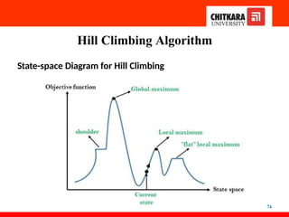
State-spaceDiagram for Hill Climbing
• The state-space landscape is a graphical representation of the
hill-climbing algorithm which is showing a graph
between various states of algorithm and Objective
function/Cost.
• On Y-axis we have taken the function which can be an objective
function or cost function, and state-space on the X-axis.
• If the function on Y-axis is cost then, the goal of the search is to
find the global minimum and local minimum.
• If the function of the Y-axis is the Objective function, then the
goal of the search is to find the global maximum and local
maximum.
Hill Climbing Algorithm
75
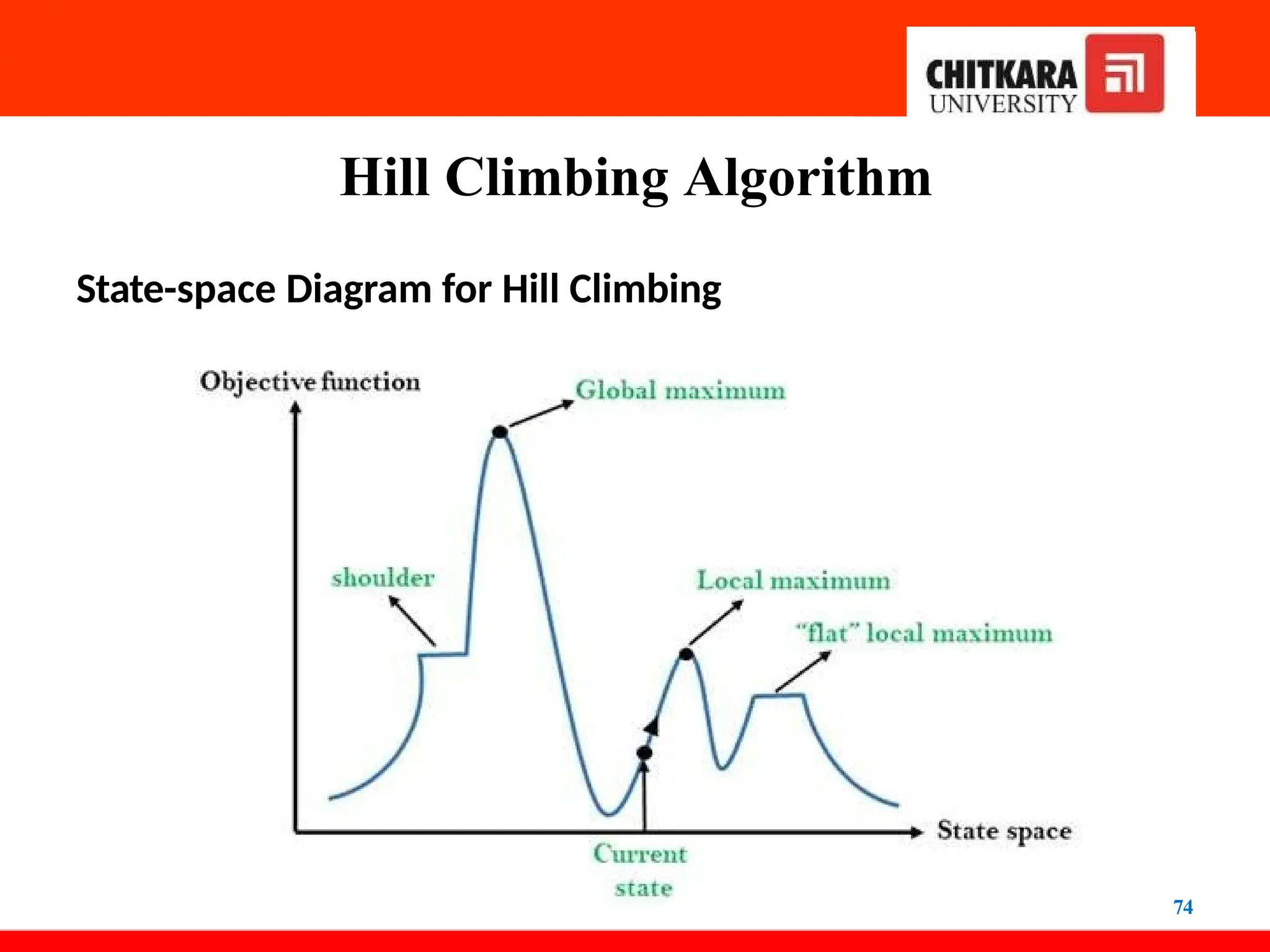
State-spaceDiagram for Hill Climbing
Local Maximum: Local maximum is a state which is better than its neighbor
states, but there is also another state which is higher than it.
Global Maximum: Global maximum is the best possible state of state space
landscape. It has the highest value of the objective function.
Current state: It is a state in a landscape diagram where an agent is currently
present.
Flat local maximum: It is a flat space in the landscape where all the neighbor
states of current states have the same value.
Shoulder: It is a plateau region that has an uphill edge.
76.
Hill Climbing Algorithm
76
•Simple hill climbing is the simplest way to implement a hill
climbing algorithm.
• It only evaluates the neighbor node state at a time and
selects the first one which optimizes current cost and
sets it as a current state.
• It only checks its one successor state, and if it finds better
than the current state, then move else be in the same state.
77.
Hill Climbing Algorithm
77
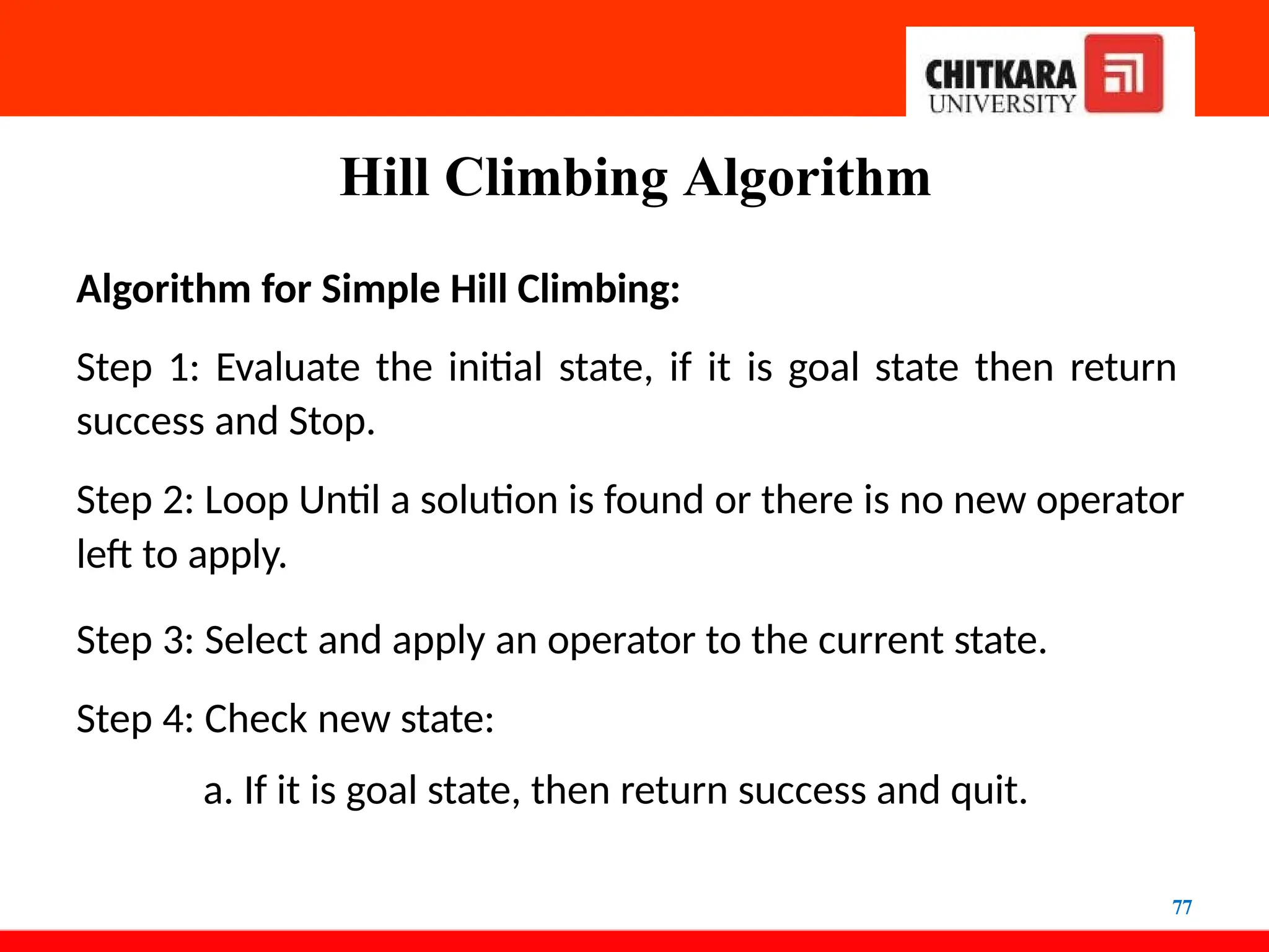
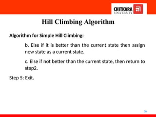
Algorithmfor Simple Hill Climbing:
Step 1: Evaluate the initial state, if it is goal state then return
success and Stop.
Step 2: Loop Until a solution is found or there is no new operator
left to apply.
Step 3: Select and apply an operator to the current state.
Step 4: Check new state:
a. If it is goal state, then return success and quit.
78.
Hill Climbing Algorithm
78
Algorithmfor Simple Hill Climbing:
b. Else if it is better than the current state then assign
new state as a current state.
c. Else if not better than the current state, then return to
step2.
Step 5: Exit.
79.
Example of HillClimbing Algorithm
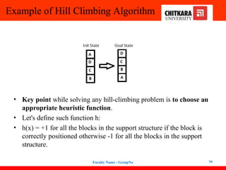
• Key point while solving any hill-climbing problem is to choose an
appropriate heuristic function.
• Let's define such function h:
• h(x) = +1 for all the blocks in the support structure if the block is
correctly positioned otherwise -1 for all the blocks in the support
structure.
Faculty Name - GroupNo 79
80.
Example of HillClimbing Algorithm
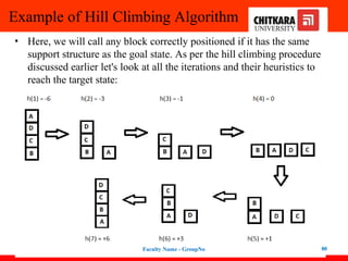
• Here, we will call any block correctly positioned if it has the same
support structure as the goal state. As per the hill climbing procedure
discussed earlier let's look at all the iterations and their heuristics to
reach the target state:
Faculty Name - GroupNo 80
81.
Means-Ends Analysis
81
• Means-EndsAnalysis is problem-solving technique used
in Artificial intelligence for limiting search in AI programs.
• It is a mixture of Backward and forward search techniques.
• The MEA analysis process centered on the evaluation of the
difference between the current state and goal state.
82.
Means-Ends Analysis
82
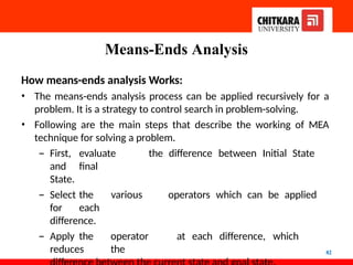
How means-endsanalysis Works:
• The means-ends analysis process can be applied recursively for a
problem. It is a strategy to control search in problem-solving.
• Following are the main steps that describe the working of MEA
technique for solving a problem.
– First, evaluate the difference between Initial State
and final
State.
– Select the various operators which can be applied
for each
difference.
– Apply the operator at each difference, which
reduces the
Means-Ends Analysis
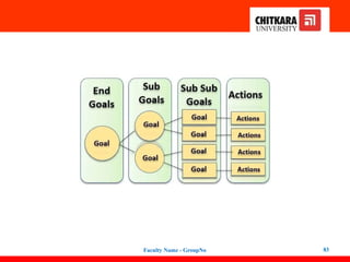
84
Operator Subgoaling
•In the MEA process, we detect the differences between the
current state and the goal state. Once these differences
occur, then we can apply an operator to reduce the
differences.
• But sometimes it is possible that an operator cannot be applied
to the current state.
• So we create the subproblem of the current state, in which
operator can be applied, such type of backward chaining
in which operators are selected, and then sub-goals are set up
to establish the preconditions of the operator is called
Subgoaling.
85.
Algorithm for Means-EndsAnalysis
85
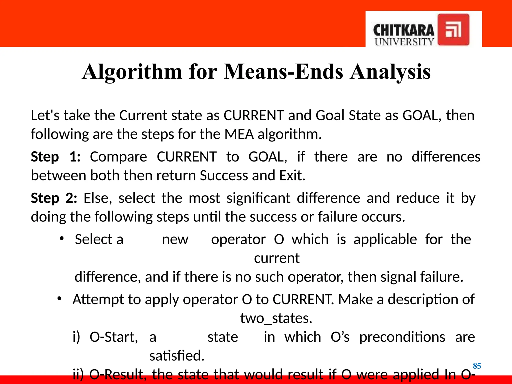
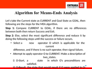
Let's take the Current state as CURRENT and Goal State as GOAL, then
following are the steps for the MEA algorithm.
Step 1: Compare CURRENT to GOAL, if there are no differences
between both then return Success and Exit.
Step 2: Else, select the most significant difference and reduce it by
doing the following steps until the success or failure occurs.
• Select a new operator O which is applicable for the
current
difference, and if there is no such operator, then signal failure.
• Attempt to apply operator O to CURRENT. Make a description of
two_states.
i) O-Start, a state in which O’s preconditions are
satisfied.
ii) O-Result, the state that would result if O were applied In O-
86.
Algorithm for Means-EndsAnalysis
86
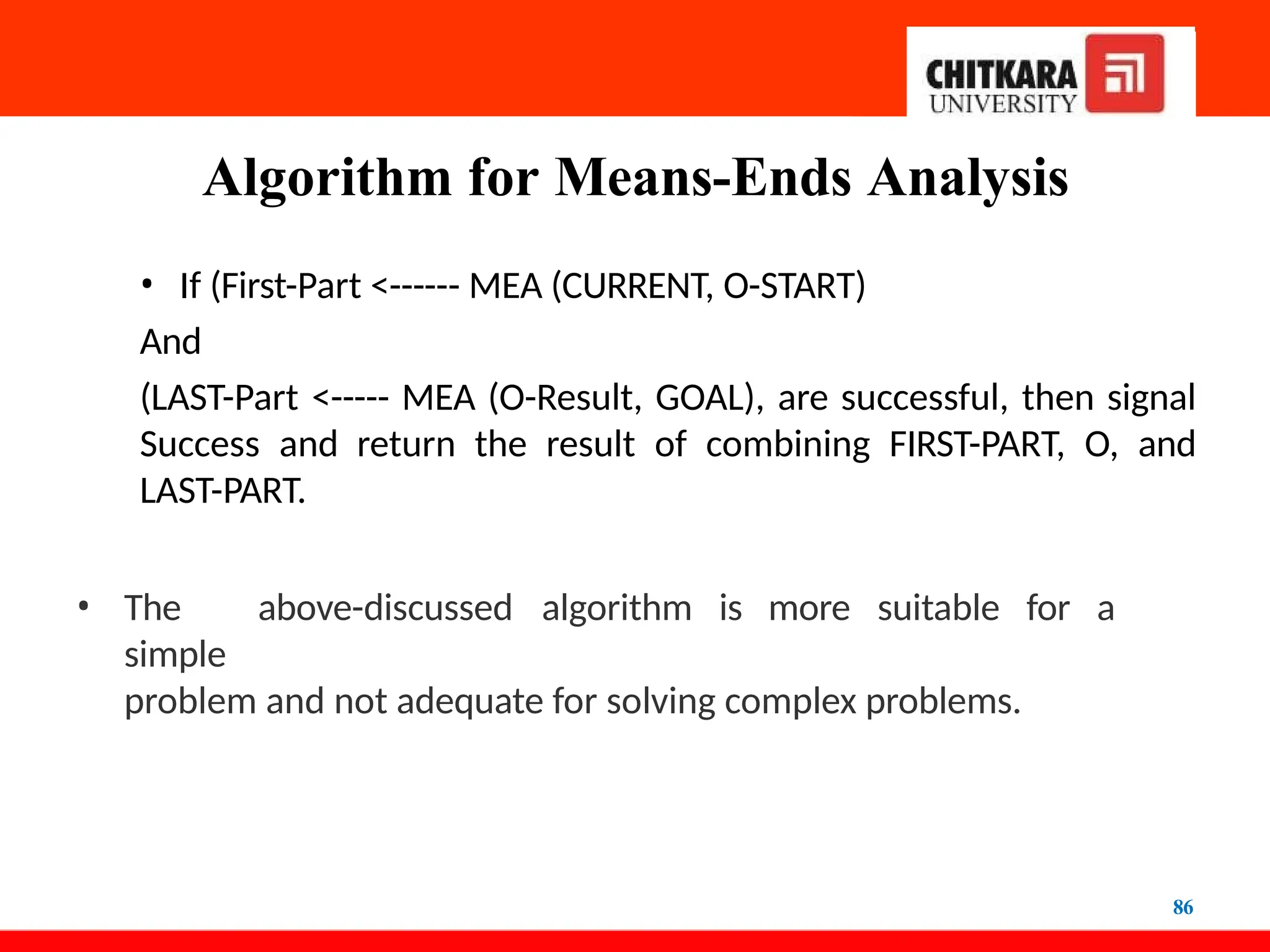
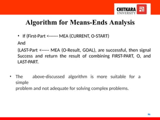
• If (First-Part <------ MEA (CURRENT, O-START)
And
(LAST-Part <----- MEA (O-Result, GOAL), are successful, then signal
Success and return the result of combining FIRST-PART, O, and
LAST-PART.
• The above-discussed algorithm is more suitable for a
simple
problem and not adequate for solving complex problems.
87.
• In Means-EndAnalysis you try to reduce the difference between
initial state and goal state by creating sub goals until a sub goal can
be reached directly (probably you know several examples of
recursion which works on the basis of this).
• An example for a problem that can be solved by Means-End
Analysis are the “Towers of Hanoi“
Faculty Name - GroupNo 87
88.
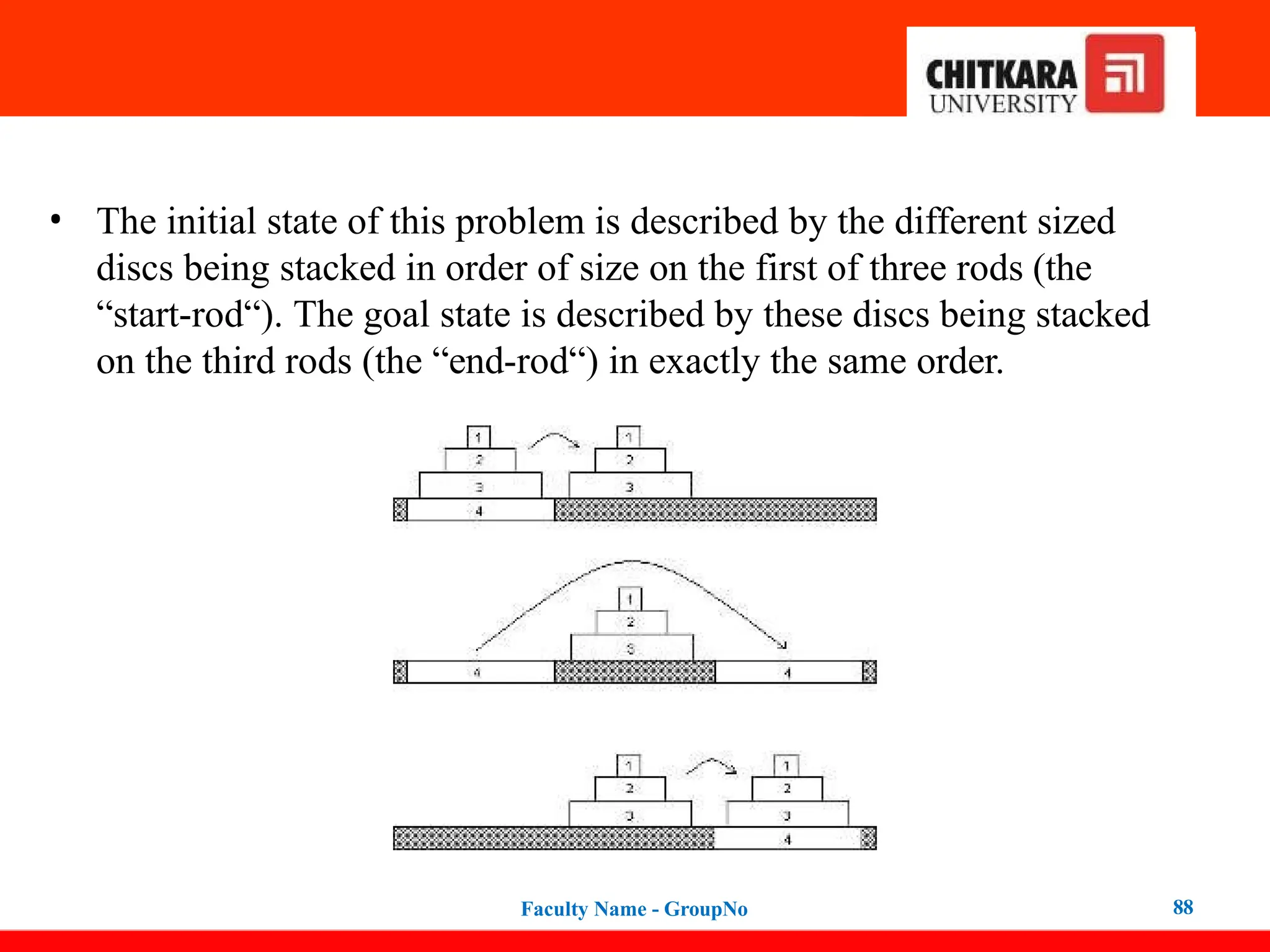
• The initialstate of this problem is described by the different sized
discs being stacked in order of size on the first of three rods (the
“start-rod“). The goal state is described by these discs being stacked
on the third rods (the “end-rod“) in exactly the same order.
Faculty Name - GroupNo 88
89.
• There arethree operators:
• You are allowed to move one single disc from one rod to another
one
• You are only able to move a disc if it is on top of one stack
• A disc cannot be put onto a smaller one.
Faculty Name - GroupNo 89
90.
• In orderto use Means-End Analysis we have to create subgoals. One
possible way of doing this is described in the picture:
• 1. Moving the discs lying on the biggest one onto the second rod.
• 2. Shifting the biggest disc to the third rod.
• 3. Moving the other ones onto the third rod, too.
Faculty Name - GroupNo 90
91.
• You canapply this strategy again and again in order to reduce the
problem to the case where you only have to move a single disc –
which is then something you are allowed to do.
• Strategies of this kind can easily be formulated for a computer;
the
respective algorithm for the Towers of Hanoi would look like
this:
1. move n-1 discs from A to B
2. move disc #n from A to C
3. move n-1 discs from B to C
• Where n is the total number of discs, A is the first rod, B the
second, C the third one. Now the problem is reduced by one with
each recursive loop.
Faculty Name - GroupNo 91
92.
• Means-end analysisis important to solve everyday-problems - like
getting the right train connection: You have to figure out where you
catch the first train and where you want to arrive, first of all. Then
you have to look for possible changes just in case you do not get a
direct connection. Third, you have to figure out what are the best
times of departure and arrival, on which platforms you leave and
arrive and make it all fit together.
Faculty Name - GroupNo 92
93.
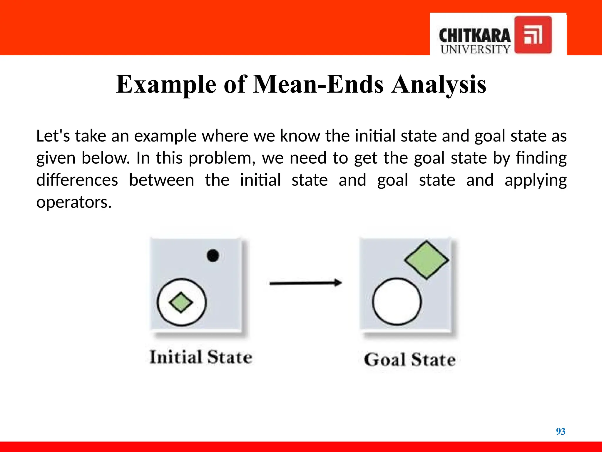
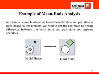
Example of Mean-EndsAnalysis
Let's take an example where we know the initial state and goal state as
given below. In this problem, we need to get the goal state by finding
differences between the initial state and goal state and applying
operators.
93
94.
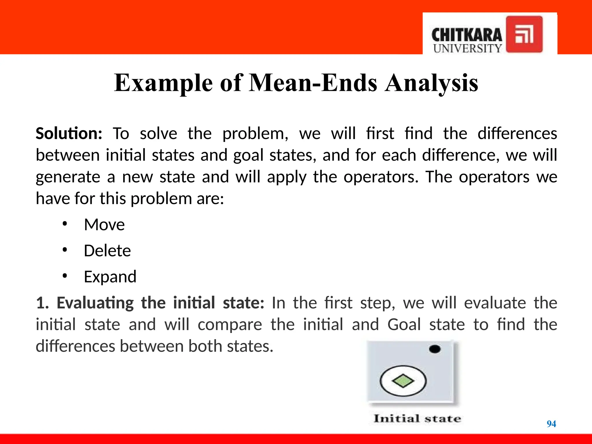
Example of Mean-EndsAnalysis
Solution: To solve the problem, we will first find the differences
between initial states and goal states, and for each difference, we will
generate a new state and will apply the operators. The operators we
have for this problem are:
• Move
• Delete
• Expand
1. Evaluating the initial state: In the first step, we will evaluate the
initial state and will compare the initial and Goal state to find the
differences between both states.
94
95.
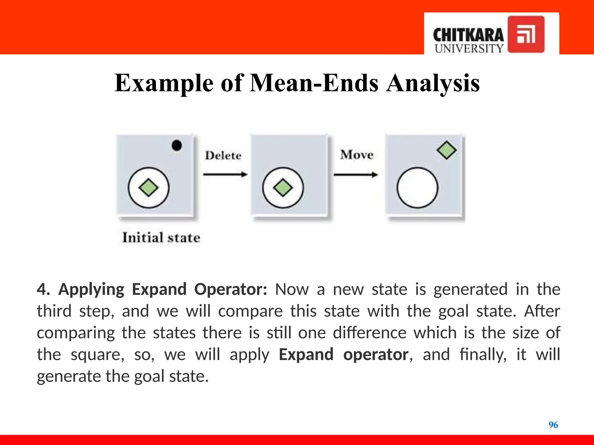
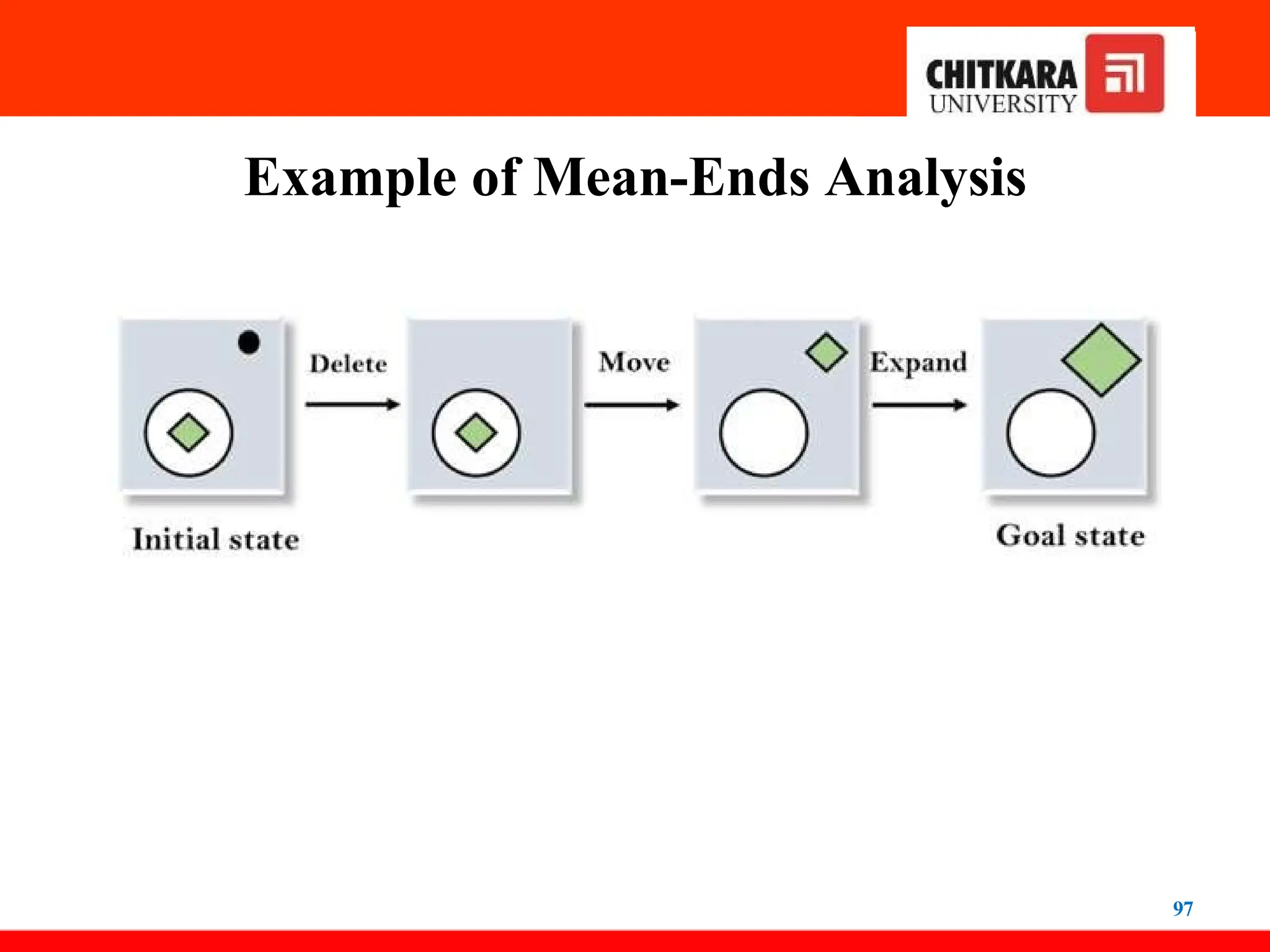
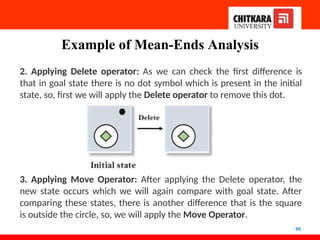
Example of Mean-EndsAnalysis
2. Applying Delete operator: As we can check the first difference is
that in goal state there is no dot symbol which is present in the initial
state, so, first we will apply the Delete operator to remove this dot.
3. Applying Move Operator: After applying the Delete operator, the
new state occurs which we will again compare with goal state. After
comparing these states, there is another difference that is the square
is outside the circle, so, we will apply the Move Operator.
95
96.
Example of Mean-EndsAnalysis
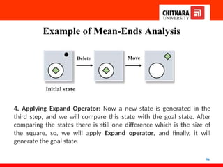
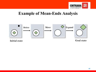
4. Applying Expand Operator: Now a new state is generated in the
third step, and we will compare this state with the goal state. After
comparing the states there is still one difference which is the size of
the square, so, we will apply Expand operator, and finally, it will
generate the goal state.
96
![Unit- 2
Introduction to Artificial
Intelligent
[22AI002]
Dr. Aditi Moudgil
Assistant Professor
Department of Computer Science and Engineering
Chitkara University, Punjab](https://image.slidesharecdn.com/unit-2-250906124210-03a95f37/85/Introduction-to-artificial-intelligence-part-2-1-320.jpg)
![Syllabus
2
Unit - 1 Introduction to Artificial Intelligence [4 hrs]
Introduction of Artificial Intelligence: Definition, Goals of AI, Applications areas of AI,
History of AI, Types of AI, Importance of Artificial Intelligence, Intelligent agents and
environment.
Unit - 2 Searching [6 hrs]
Searching: Search algorithm terminologies, properties for search algorithms, Search
Algorithms, Uninformed Search Algorithms, Informed Search Algorithms, Hill Climbing
Algorithm, Means-Ends Analysis.
Unit - 3 Knowledge [9 hrs]
Knowledge-Based Agent, Architecture of knowledge-based agent, Inference system,
Operations performed by Knowledge-Based Agent, Knowledge Representation, Types
of Knowledge, Approaches to knowledge representation, Knowledge Representation
Techniques.](https://image.slidesharecdn.com/unit-2-250906124210-03a95f37/85/Introduction-to-artificial-intelligence-part-2-2-320.jpg)
![Syllabus
3
Unit - 4 Logic [11 hrs]
Propositional Logic, Rules of Inference, The Wumpus world, knowledge-base for
Wumpus World, First-order logic, Knowledge Engineering in FOL, Inference in First-
Order Logic, Unification in FOL, Resolution in FOL, Forward Chaining and backward
chaining, Backward Chaining vs forwarding Chaining, Reasoning in AI, Inductive vs.
Deductive reasoning.
Textbooks
1.Introduction to Artificial Intelligence & Expert Systems' by Dan W.
Patterson, Englewood Cliffs, NJ, 1990, Prentice-Hall International.
Reference Books
2. 'Artificial Intelligence’ by Elaine Rich, Kevin Knight, Shivashankar B Nair, (McGraw-
Hill)
2. ‘Artificial Intelligence A Modern Approach, ‘ by Stuart J. Russell and Peter
Norvig, Third Edition, Prentice-Hall.](https://image.slidesharecdn.com/unit-2-250906124210-03a95f37/85/Introduction-to-artificial-intelligence-part-2-3-320.jpg)
![Contents
4
Unit -2 Searching [6 hrs]
• Search Algorithm Terminologies,
• Properties For Search Algorithms,
• Search Algorithms,
• Uninformed Search Algorithms,
• Informed Search Algorithms,
• Hill Climbing Algorithm,
• Means-ends Analysis.](https://image.slidesharecdn.com/unit-2-250906124210-03a95f37/85/Introduction-to-artificial-intelligence-part-2-4-320.jpg)


![Depth-first Search Pseudocode
22
DFS(G, u)
u.visited = true
for each v ∈
G.Adj[u]
if v.visited == false
DFS(G,v)
init() {
For each u ∈ G
u.visited = false
For each u ∈ G
DFS(G, u)
}](https://image.slidesharecdn.com/unit-2-250906124210-03a95f37/85/Introduction-to-artificial-intelligence-part-2-22-320.jpg)


![Best-first Search Algorithm (Greedy Search)
48
Expand the nodes of S and put in the CLOSED list
Initialization: Open [B, A], Closed [S]
Iteration 1: Open [A], Closed [S, B]
Iteration 2: Open [E, F, A], Closed [S, B]
: Open [F, A], Closed [S, B, E]
Iteration 3: Open [F, A], Closed [S, B, E]
: Open [A], Closed [S, B, E, F]
Iteration 4: Open [G, I, A], Closed [S, B,
E, F]
: Open [I, A], Closed [S, B, E,
F, G]
Hence the final solution path will be:
S----> B----->F----> G](https://image.slidesharecdn.com/unit-2-250906124210-03a95f37/85/Introduction-to-artificial-intelligence-part-2-48-320.jpg)


![Unit- 2
Introduction to Artificial
Intelligent
[22AI002]
Dr. Aditi Moudgil
Assistant Professor
Department of Computer Science and Engineering
Chitkara University, Punjab](https://image.slidesharecdn.com/unit-2-250906124210-03a95f37/75/Introduction-to-artificial-intelligence-part-2-1-2048.jpg)
![Syllabus
2
Unit - 1 Introduction to Artificial Intelligence [4 hrs]
Introduction of Artificial Intelligence: Definition, Goals of AI, Applications areas of AI,
History of AI, Types of AI, Importance of Artificial Intelligence, Intelligent agents and
environment.
Unit - 2 Searching [6 hrs]
Searching: Search algorithm terminologies, properties for search algorithms, Search
Algorithms, Uninformed Search Algorithms, Informed Search Algorithms, Hill Climbing
Algorithm, Means-Ends Analysis.
Unit - 3 Knowledge [9 hrs]
Knowledge-Based Agent, Architecture of knowledge-based agent, Inference system,
Operations performed by Knowledge-Based Agent, Knowledge Representation, Types
of Knowledge, Approaches to knowledge representation, Knowledge Representation
Techniques.](https://image.slidesharecdn.com/unit-2-250906124210-03a95f37/75/Introduction-to-artificial-intelligence-part-2-2-2048.jpg)
![Syllabus
3
Unit - 4 Logic [11 hrs]
Propositional Logic, Rules of Inference, The Wumpus world, knowledge-base for
Wumpus World, First-order logic, Knowledge Engineering in FOL, Inference in First-
Order Logic, Unification in FOL, Resolution in FOL, Forward Chaining and backward
chaining, Backward Chaining vs forwarding Chaining, Reasoning in AI, Inductive vs.
Deductive reasoning.
Textbooks
1.Introduction to Artificial Intelligence & Expert Systems' by Dan W.
Patterson, Englewood Cliffs, NJ, 1990, Prentice-Hall International.
Reference Books
2. 'Artificial Intelligence’ by Elaine Rich, Kevin Knight, Shivashankar B Nair, (McGraw-
Hill)
2. ‘Artificial Intelligence A Modern Approach, ‘ by Stuart J. Russell and Peter
Norvig, Third Edition, Prentice-Hall.](https://image.slidesharecdn.com/unit-2-250906124210-03a95f37/75/Introduction-to-artificial-intelligence-part-2-3-2048.jpg)
![Contents
4
Unit -2 Searching [6 hrs]
• Search Algorithm Terminologies,
• Properties For Search Algorithms,
• Search Algorithms,
• Uninformed Search Algorithms,
• Informed Search Algorithms,
• Hill Climbing Algorithm,
• Means-ends Analysis.](https://image.slidesharecdn.com/unit-2-250906124210-03a95f37/75/Introduction-to-artificial-intelligence-part-2-4-2048.jpg)


![Depth-first Search Pseudocode
22
DFS(G, u)
u.visited = true
for each v ∈
G.Adj[u]
if v.visited == false
DFS(G,v)
init() {
For each u ∈ G
u.visited = false
For each u ∈ G
DFS(G, u)
}](https://image.slidesharecdn.com/unit-2-250906124210-03a95f37/75/Introduction-to-artificial-intelligence-part-2-22-2048.jpg)


![Best-first Search Algorithm (Greedy Search)
48
Expand the nodes of S and put in the CLOSED list
Initialization: Open [B, A], Closed [S]
Iteration 1: Open [A], Closed [S, B]
Iteration 2: Open [E, F, A], Closed [S, B]
: Open [F, A], Closed [S, B, E]
Iteration 3: Open [F, A], Closed [S, B, E]
: Open [A], Closed [S, B, E, F]
Iteration 4: Open [G, I, A], Closed [S, B,
E, F]
: Open [I, A], Closed [S, B, E,
F, G]
Hence the final solution path will be:
S----> B----->F----> G](https://image.slidesharecdn.com/unit-2-250906124210-03a95f37/75/Introduction-to-artificial-intelligence-part-2-48-2048.jpg)