Downloaded 605 times


![Entering Matrices (1) >> A = [1 2 3; 4 5 6; 7 8 9] OR >> A = [ 1 2 3 4 5 6 7 8 9 ]](https://image.slidesharecdn.com/matlabnotes-110104184012-phpapp01/85/Introduction-to-MatLab-programming-12-320.jpg)
![Complex Matrices To enter a complex matrix, you may do it in one of two ways : >> A = [1 2; 3 4] + i*[5 6;7 8] OR >> A = [1+5i 2+6i; 3+7i 4+8i]](https://image.slidesharecdn.com/matlabnotes-110104184012-phpapp01/85/Introduction-to-MatLab-programming-15-320.jpg)
![Matrix Addition » A = [ 1 1 1 ; 2 2 2 ; 3 3 3] » B = [3 3 3 ; 4 4 4 ; 5 5 5 ] » A + B ans = 4 4 4 6 6 6 8 8 8](https://image.slidesharecdn.com/matlabnotes-110104184012-phpapp01/85/Introduction-to-MatLab-programming-17-320.jpg)
![Matrix Subtraction » A = [ 1 1 1 ; 2 2 2 ; 3 3 3] » B = [3 3 3 ; 4 4 4 ; 5 5 5 ] » B - A ans = 2 2 2 2 2 2 2 2 2](https://image.slidesharecdn.com/matlabnotes-110104184012-phpapp01/85/Introduction-to-MatLab-programming-18-320.jpg)
![Matrix Multiplication » A = [ 1 1 1 ; 2 2 2 ; 3 3 3] » B = [3 3 3 ; 4 4 4 ; 5 5 5 ] » A * B ans = 12 12 12 24 24 24 36 36 36](https://image.slidesharecdn.com/matlabnotes-110104184012-phpapp01/85/Introduction-to-MatLab-programming-19-320.jpg)


![Concatenation To create a large matrix from a group of smaller ones try A = magic(3) B = [ A, zeros(3,2) ; zeros(2,3), eye(2)] C = [A A+32 ; A+48 A+16] Try some of your own !!](https://image.slidesharecdn.com/matlabnotes-110104184012-phpapp01/85/Introduction-to-MatLab-programming-35-320.jpg)


![Deleting Rows and Columns (1) Create a temporary matrix X X=A; X(:, 2) = [] Deleting a single element won’t result in a matrix, so the following will return an error X(1,2) = []](https://image.slidesharecdn.com/matlabnotes-110104184012-phpapp01/85/Introduction-to-MatLab-programming-42-320.jpg)
![Deleting Rows and Columns (2) However, using a single subscript, you can delete a single element sequence of elements So X(2:2:10) = [] gives x = 16 9 2 7 13 12 1](https://image.slidesharecdn.com/matlabnotes-110104184012-phpapp01/85/Introduction-to-MatLab-programming-43-320.jpg)
![The ‘FIND’ Command (2) A = [ 1 2 3 ; 4 5 6 ; 7 8 9] [i, j] = find (A > 5) i = 3 3 2 3 j = 1 2 3 3](https://image.slidesharecdn.com/matlabnotes-110104184012-phpapp01/85/Introduction-to-MatLab-programming-45-320.jpg)
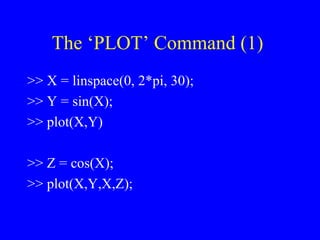
![The ‘PLOT’ Command (2) >> W = [Y ; Z] >> plot (X,W) Rotate by 90 degrees >> plot(W,X)](https://image.slidesharecdn.com/matlabnotes-110104184012-phpapp01/85/Introduction-to-MatLab-programming-49-320.jpg)


![The ‘PLOT’ Command (2) >> W = [Y ; Z] >> plot (X,W) Rotate by 90 degrees >> plot(W,X)](https://image.slidesharecdn.com/matlabnotes-110104184012-phpapp01/85/Introduction-to-MatLab-programming-52-320.jpg)
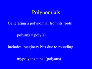
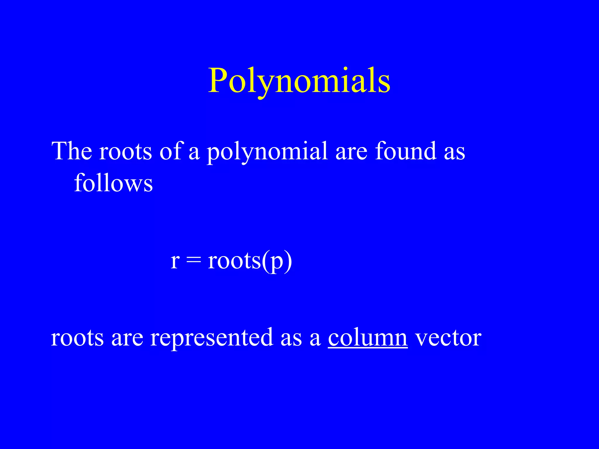
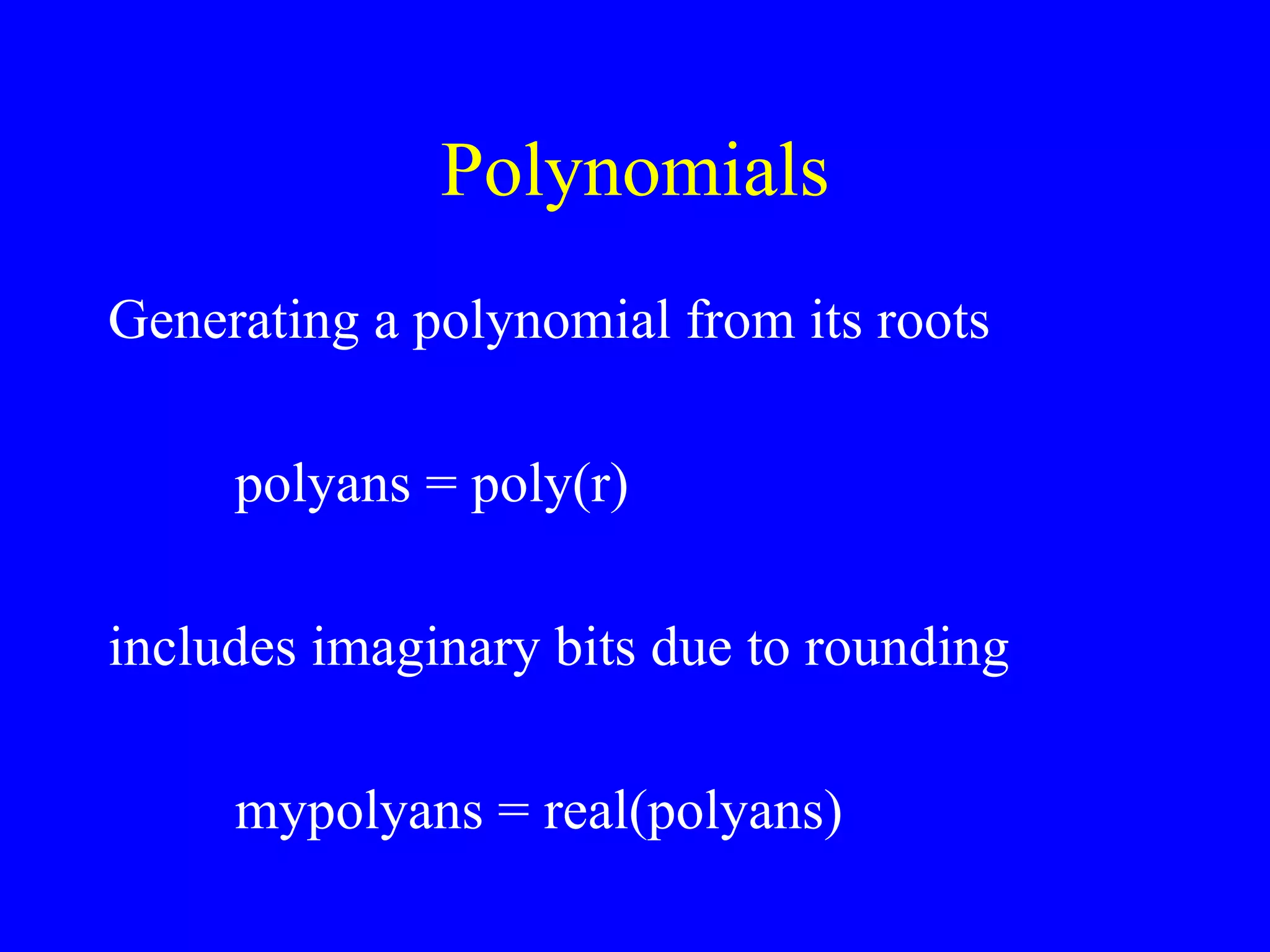
![Polynomials Polynomials are represented as row vectors with its coefficients in descending order, e.g. X 4 - 12X 3 + 0X 2 +25X + 116 p = [1 -12 0 25 116]](https://image.slidesharecdn.com/matlabnotes-110104184012-phpapp01/85/Introduction-to-MatLab-programming-57-320.jpg)

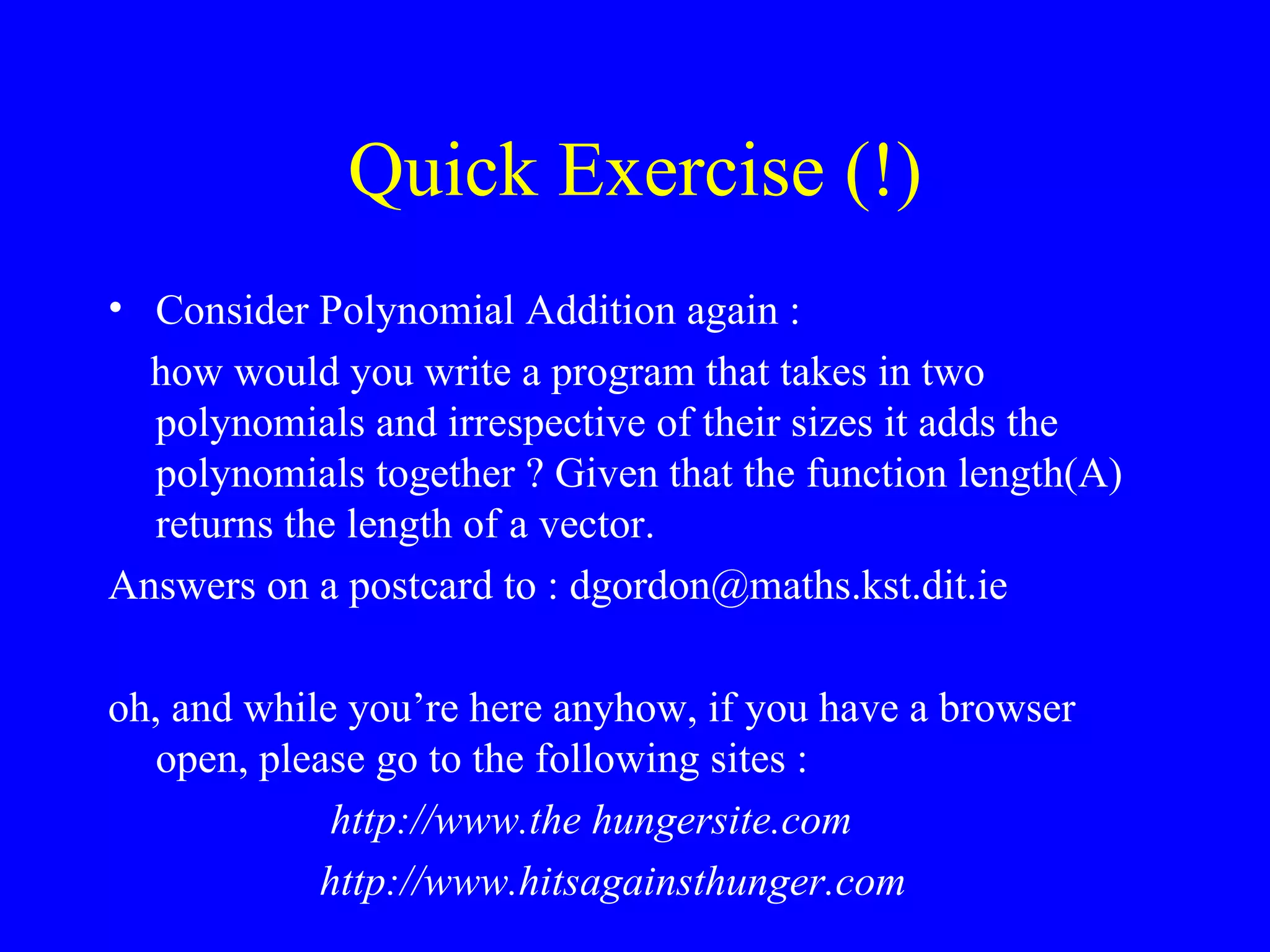
![Polynomial Addition/Sub a = [1 2 3 4] b = [1 4 9 16] c = a + b d = b - a](https://image.slidesharecdn.com/matlabnotes-110104184012-phpapp01/85/Introduction-to-MatLab-programming-60-320.jpg)
![Polynomial Addition/Sub What if two polynomials of different order ? X 3 + 2X 2 +3X + 4 X 6 + 6X 5 + 20X 4 - 52X 3 + 81X 2 +96X + 84 a = [1 2 3 4] e = [1 6 20 52 81 96 84] f = e + [0 0 0 a] or f = e + [zeros(1,3) a]](https://image.slidesharecdn.com/matlabnotes-110104184012-phpapp01/85/Introduction-to-MatLab-programming-61-320.jpg)
![Polynomial Multiplication a = [1 2 3 4] b = [1 4 9 16] Perform the convolution of two arrays ! g = conv(a,b) g = 1 6 20 50 75 84 64](https://image.slidesharecdn.com/matlabnotes-110104184012-phpapp01/85/Introduction-to-MatLab-programming-62-320.jpg)
![Polynomial Division a = [1 2 3 4] g = [1 6 20 50 75 84 64] Perform the deconvolution of two arrays ! [q,r] = deconv(g, a) q = {quotient} 1 4 9 16 r = {remainder} 0 0 0 0 0 0 0 0](https://image.slidesharecdn.com/matlabnotes-110104184012-phpapp01/85/Introduction-to-MatLab-programming-63-320.jpg)
![Polynomial Differentiation f = [1 6 20 48 69 72 44] h = polyder(f) h = 6 30 80 144 138 72](https://image.slidesharecdn.com/matlabnotes-110104184012-phpapp01/85/Introduction-to-MatLab-programming-64-320.jpg)
![Polynomial Evaluation x = linspace(-1,3) p = [1 4 -7 -10] v = polyval(p,x) plot (x,v), title(‘Graph of P’)](https://image.slidesharecdn.com/matlabnotes-110104184012-phpapp01/85/Introduction-to-MatLab-programming-65-320.jpg)

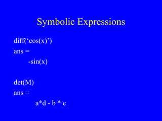
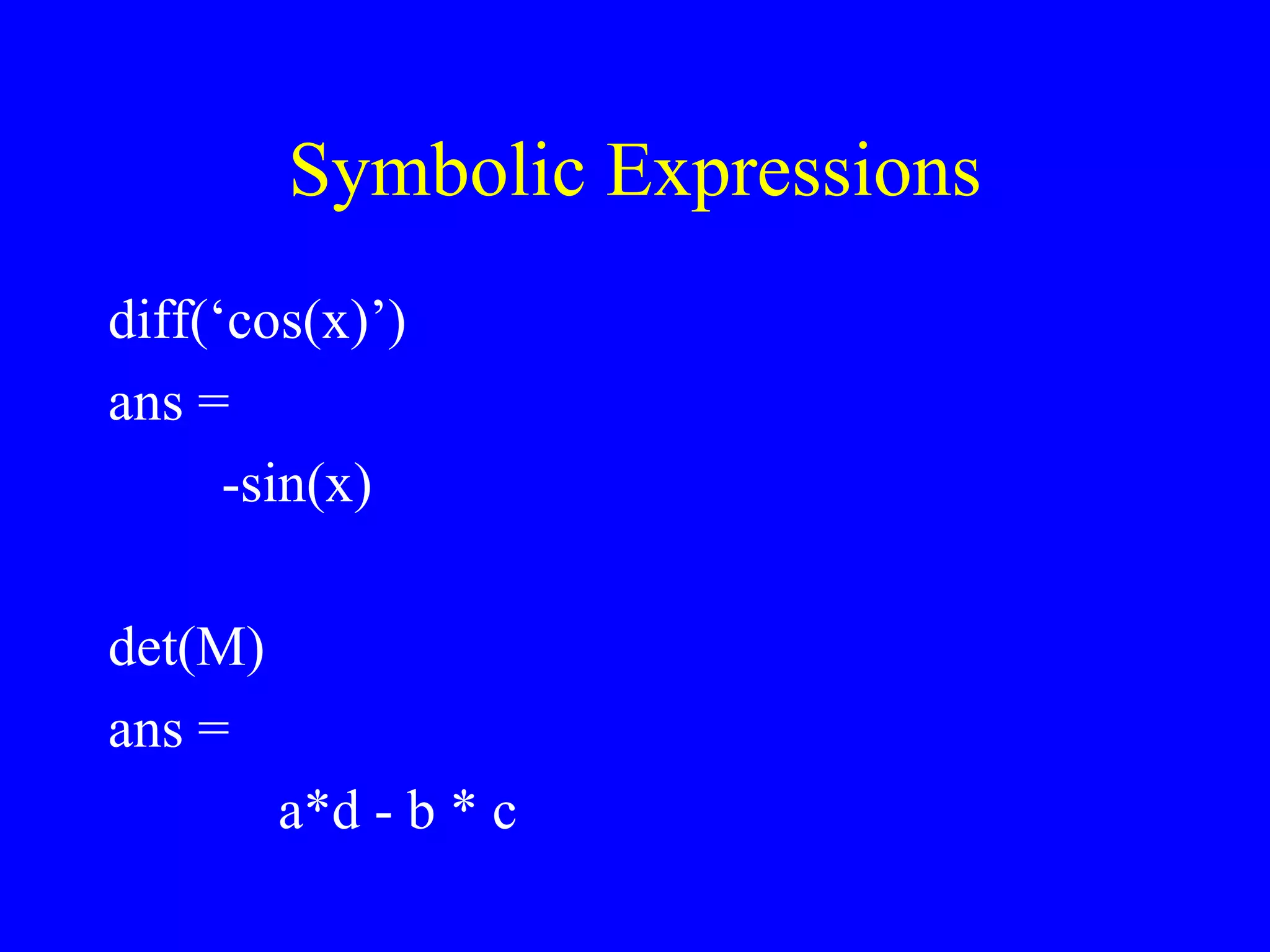
![Symbolic Expressions ‘ 1/(2*x^n)’ cos(x^2) - sin(x^2) M = sym(‘[a , b ; c , d]’) f = int(‘x^3 / sqrt(1 - x)’, ‘a’, ‘b’)](https://image.slidesharecdn.com/matlabnotes-110104184012-phpapp01/85/Introduction-to-MatLab-programming-71-320.jpg)

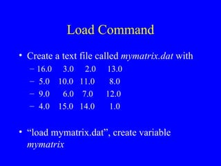
![M-Files To store your own MatLab commands in a file, create it as a text file and save it with a name that ends with “.m” So mymatrix.m A = [… 16.0 3.0 2.0 13.0 5.0 10.0 11.0 8.0 9.0 6.0 7.0 12.0 4.0 15.0 14.0 1.0]; type mymatrix](https://image.slidesharecdn.com/matlabnotes-110104184012-phpapp01/85/Introduction-to-MatLab-programming-83-320.jpg)


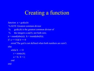


![Quick Answer (!) function c = mypoly(a,b) % MYPOLY Add two polynomials of variable lengths % mypoly(a,b) add the polynomial A to the polynomial % B, even if they are of different length % % Author: Damian Gordon % Date : 3/5/2001 % Mod'd : x/x/2001 % c = [zeros(1,length(b) - length(a)) a] + [zeros(1, length(a) - length(b)) b];](https://image.slidesharecdn.com/matlabnotes-110104184012-phpapp01/85/Introduction-to-MatLab-programming-93-320.jpg)
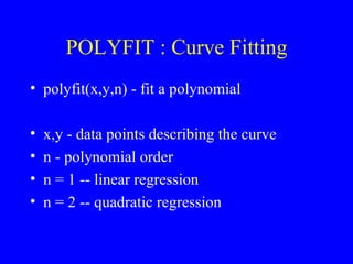
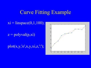
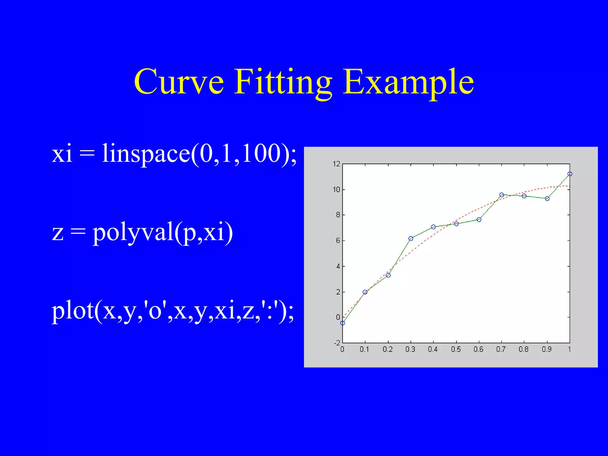
![Curve Fitting Example x = [0 .1 .2 .3 .4 .5 .6 .7 .8 .9 1]; y = [-.447 1.978 3.28 6.16 7.08 7.34 7.66 9.56 9.48 9.30 11.2]; polyfit(x,y,n) n = 1 p = 10.3185 1.4400 n = 2 p = -9.8108 20.1293 -0.0317 y = -9.8108x 2 + 20.1293x - 0.0317](https://image.slidesharecdn.com/matlabnotes-110104184012-phpapp01/85/Introduction-to-MatLab-programming-97-320.jpg)


![Entering Matrices (1) >> A = [1 2 3; 4 5 6; 7 8 9] OR >> A = [ 1 2 3 4 5 6 7 8 9 ]](https://image.slidesharecdn.com/matlabnotes-110104184012-phpapp01/75/Introduction-to-MatLab-programming-12-2048.jpg)
![Complex Matrices To enter a complex matrix, you may do it in one of two ways : >> A = [1 2; 3 4] + i*[5 6;7 8] OR >> A = [1+5i 2+6i; 3+7i 4+8i]](https://image.slidesharecdn.com/matlabnotes-110104184012-phpapp01/75/Introduction-to-MatLab-programming-15-2048.jpg)
![Matrix Addition » A = [ 1 1 1 ; 2 2 2 ; 3 3 3] » B = [3 3 3 ; 4 4 4 ; 5 5 5 ] » A + B ans = 4 4 4 6 6 6 8 8 8](https://image.slidesharecdn.com/matlabnotes-110104184012-phpapp01/75/Introduction-to-MatLab-programming-17-2048.jpg)
![Matrix Subtraction » A = [ 1 1 1 ; 2 2 2 ; 3 3 3] » B = [3 3 3 ; 4 4 4 ; 5 5 5 ] » B - A ans = 2 2 2 2 2 2 2 2 2](https://image.slidesharecdn.com/matlabnotes-110104184012-phpapp01/75/Introduction-to-MatLab-programming-18-2048.jpg)
![Matrix Multiplication » A = [ 1 1 1 ; 2 2 2 ; 3 3 3] » B = [3 3 3 ; 4 4 4 ; 5 5 5 ] » A * B ans = 12 12 12 24 24 24 36 36 36](https://image.slidesharecdn.com/matlabnotes-110104184012-phpapp01/75/Introduction-to-MatLab-programming-19-2048.jpg)

![Concatenation To create a large matrix from a group of smaller ones try A = magic(3) B = [ A, zeros(3,2) ; zeros(2,3), eye(2)] C = [A A+32 ; A+48 A+16] Try some of your own !!](https://image.slidesharecdn.com/matlabnotes-110104184012-phpapp01/75/Introduction-to-MatLab-programming-35-2048.jpg)


![Deleting Rows and Columns (1) Create a temporary matrix X X=A; X(:, 2) = [] Deleting a single element won’t result in a matrix, so the following will return an error X(1,2) = []](https://image.slidesharecdn.com/matlabnotes-110104184012-phpapp01/75/Introduction-to-MatLab-programming-42-2048.jpg)
![Deleting Rows and Columns (2) However, using a single subscript, you can delete a single element sequence of elements So X(2:2:10) = [] gives x = 16 9 2 7 13 12 1](https://image.slidesharecdn.com/matlabnotes-110104184012-phpapp01/75/Introduction-to-MatLab-programming-43-2048.jpg)
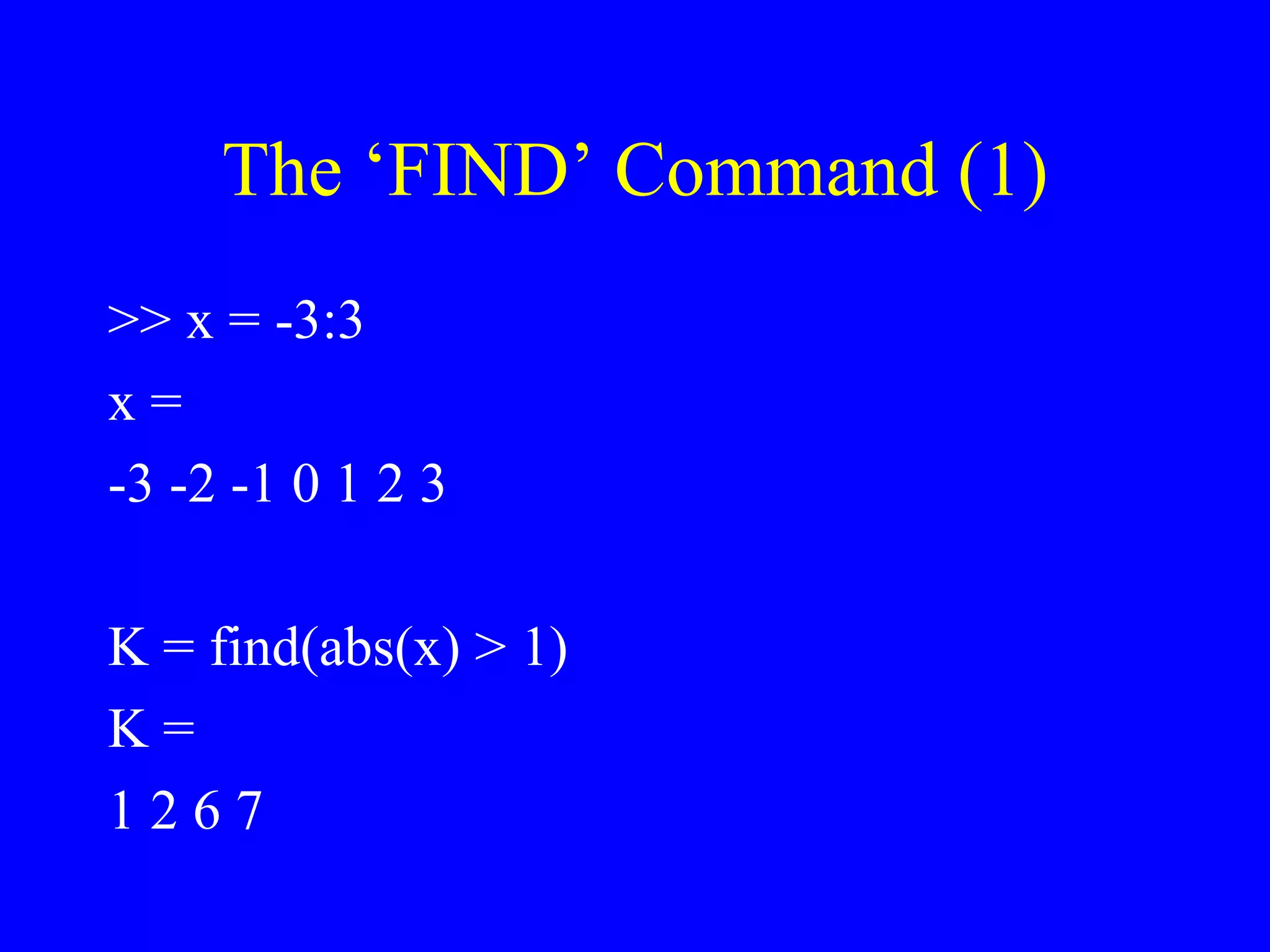
![The ‘FIND’ Command (2) A = [ 1 2 3 ; 4 5 6 ; 7 8 9] [i, j] = find (A > 5) i = 3 3 2 3 j = 1 2 3 3](https://image.slidesharecdn.com/matlabnotes-110104184012-phpapp01/75/Introduction-to-MatLab-programming-45-2048.jpg)

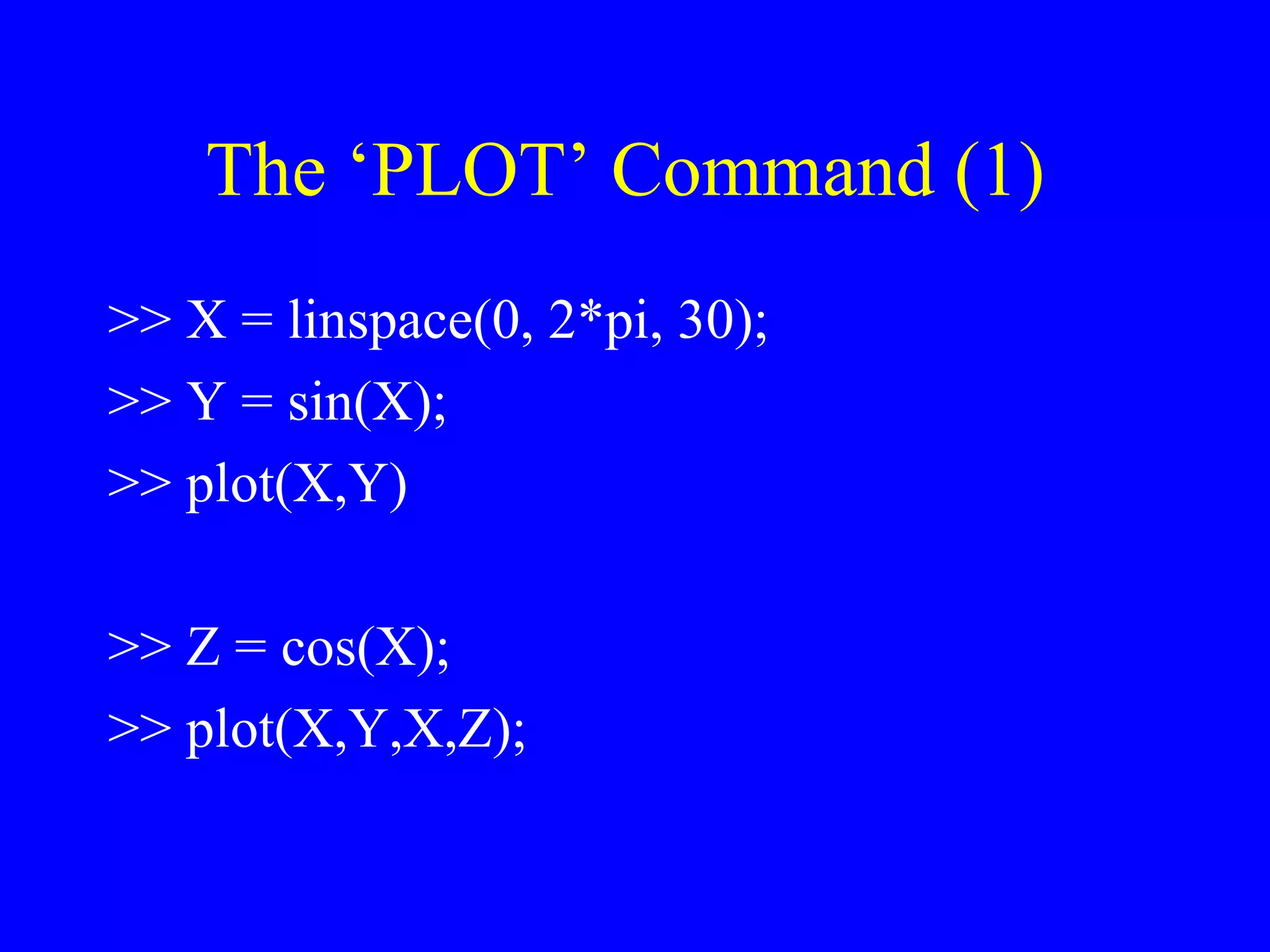
![The ‘PLOT’ Command (2) >> W = [Y ; Z] >> plot (X,W) Rotate by 90 degrees >> plot(W,X)](https://image.slidesharecdn.com/matlabnotes-110104184012-phpapp01/75/Introduction-to-MatLab-programming-49-2048.jpg)


![The ‘PLOT’ Command (2) >> W = [Y ; Z] >> plot (X,W) Rotate by 90 degrees >> plot(W,X)](https://image.slidesharecdn.com/matlabnotes-110104184012-phpapp01/75/Introduction-to-MatLab-programming-52-2048.jpg)

![Polynomials Polynomials are represented as row vectors with its coefficients in descending order, e.g. X 4 - 12X 3 + 0X 2 +25X + 116 p = [1 -12 0 25 116]](https://image.slidesharecdn.com/matlabnotes-110104184012-phpapp01/75/Introduction-to-MatLab-programming-57-2048.jpg)
![Polynomial Addition/Sub a = [1 2 3 4] b = [1 4 9 16] c = a + b d = b - a](https://image.slidesharecdn.com/matlabnotes-110104184012-phpapp01/75/Introduction-to-MatLab-programming-60-2048.jpg)
![Polynomial Addition/Sub What if two polynomials of different order ? X 3 + 2X 2 +3X + 4 X 6 + 6X 5 + 20X 4 - 52X 3 + 81X 2 +96X + 84 a = [1 2 3 4] e = [1 6 20 52 81 96 84] f = e + [0 0 0 a] or f = e + [zeros(1,3) a]](https://image.slidesharecdn.com/matlabnotes-110104184012-phpapp01/75/Introduction-to-MatLab-programming-61-2048.jpg)
![Polynomial Multiplication a = [1 2 3 4] b = [1 4 9 16] Perform the convolution of two arrays ! g = conv(a,b) g = 1 6 20 50 75 84 64](https://image.slidesharecdn.com/matlabnotes-110104184012-phpapp01/75/Introduction-to-MatLab-programming-62-2048.jpg)
![Polynomial Division a = [1 2 3 4] g = [1 6 20 50 75 84 64] Perform the deconvolution of two arrays ! [q,r] = deconv(g, a) q = {quotient} 1 4 9 16 r = {remainder} 0 0 0 0 0 0 0 0](https://image.slidesharecdn.com/matlabnotes-110104184012-phpapp01/75/Introduction-to-MatLab-programming-63-2048.jpg)
![Polynomial Differentiation f = [1 6 20 48 69 72 44] h = polyder(f) h = 6 30 80 144 138 72](https://image.slidesharecdn.com/matlabnotes-110104184012-phpapp01/75/Introduction-to-MatLab-programming-64-2048.jpg)
![Polynomial Evaluation x = linspace(-1,3) p = [1 4 -7 -10] v = polyval(p,x) plot (x,v), title(‘Graph of P’)](https://image.slidesharecdn.com/matlabnotes-110104184012-phpapp01/75/Introduction-to-MatLab-programming-65-2048.jpg)


![Symbolic Expressions ‘ 1/(2*x^n)’ cos(x^2) - sin(x^2) M = sym(‘[a , b ; c , d]’) f = int(‘x^3 / sqrt(1 - x)’, ‘a’, ‘b’)](https://image.slidesharecdn.com/matlabnotes-110104184012-phpapp01/75/Introduction-to-MatLab-programming-71-2048.jpg)


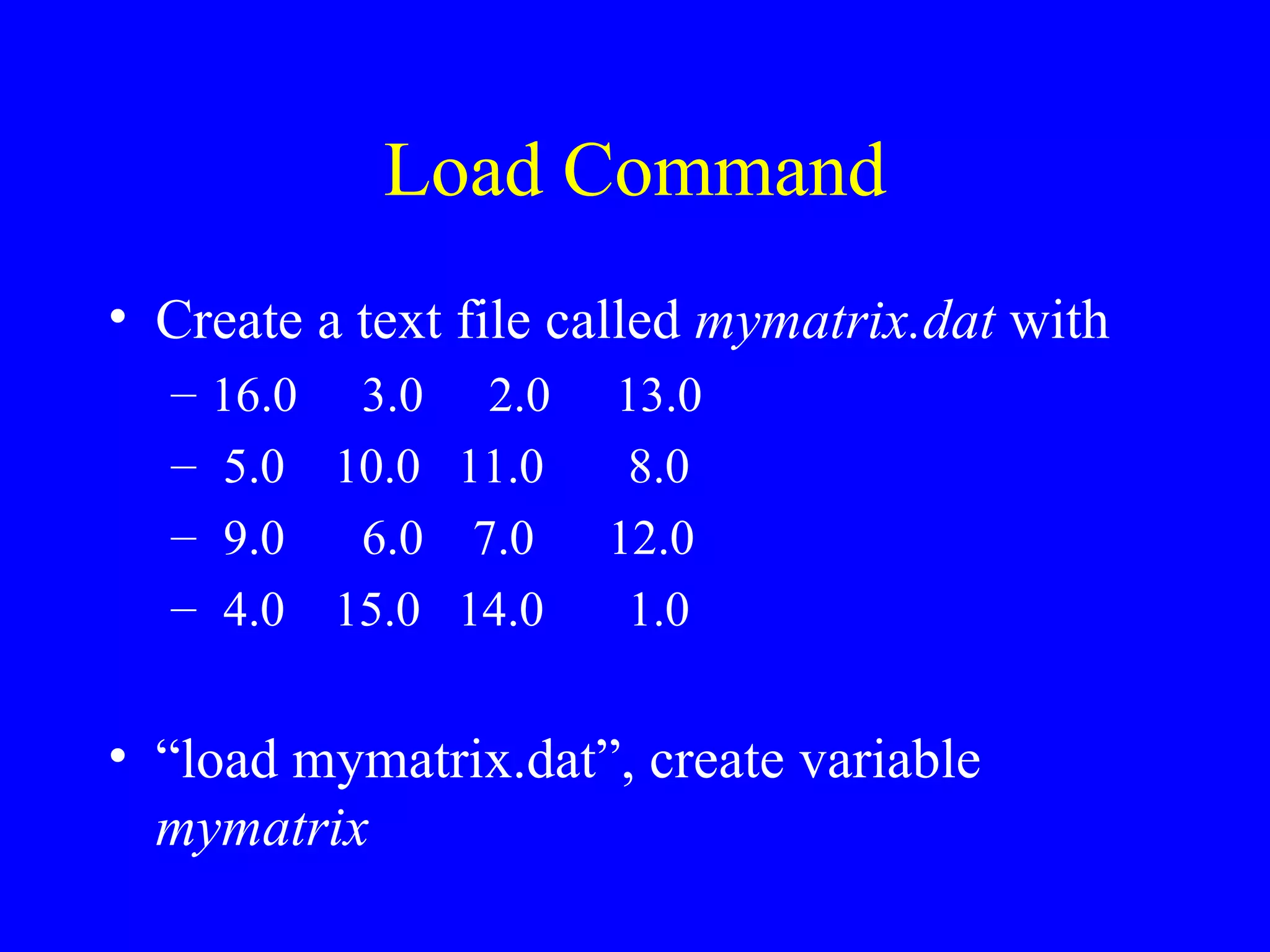
![M-Files To store your own MatLab commands in a file, create it as a text file and save it with a name that ends with “.m” So mymatrix.m A = [… 16.0 3.0 2.0 13.0 5.0 10.0 11.0 8.0 9.0 6.0 7.0 12.0 4.0 15.0 14.0 1.0]; type mymatrix](https://image.slidesharecdn.com/matlabnotes-110104184012-phpapp01/75/Introduction-to-MatLab-programming-83-2048.jpg)


![Quick Answer (!) function c = mypoly(a,b) % MYPOLY Add two polynomials of variable lengths % mypoly(a,b) add the polynomial A to the polynomial % B, even if they are of different length % % Author: Damian Gordon % Date : 3/5/2001 % Mod'd : x/x/2001 % c = [zeros(1,length(b) - length(a)) a] + [zeros(1, length(a) - length(b)) b];](https://image.slidesharecdn.com/matlabnotes-110104184012-phpapp01/75/Introduction-to-MatLab-programming-93-2048.jpg)
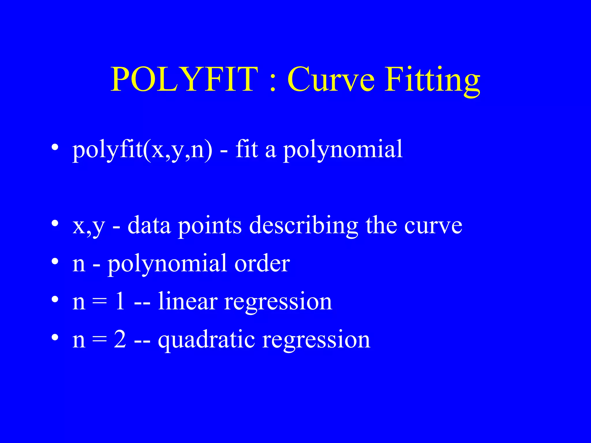
![Curve Fitting Example x = [0 .1 .2 .3 .4 .5 .6 .7 .8 .9 1]; y = [-.447 1.978 3.28 6.16 7.08 7.34 7.66 9.56 9.48 9.30 11.2]; polyfit(x,y,n) n = 1 p = 10.3185 1.4400 n = 2 p = -9.8108 20.1293 -0.0317 y = -9.8108x 2 + 20.1293x - 0.0317](https://image.slidesharecdn.com/matlabnotes-110104184012-phpapp01/75/Introduction-to-MatLab-programming-97-2048.jpg)


This document provides an introduction and overview of MATLAB (Matrix Laboratory), an interactive program for numerical computation and visualization. It discusses basic MATLAB commands and functions for creating variables and matrices, performing mathematical operations, plotting graphs, and working with polynomials.


