Introduction: Definition
• Patternrecognition is the theory or algorithm concerned
with the automatic detection (recognition) and later
classification of objects or events using a machine/computer.
2.
• Applications ofPattern Recognition
• Some examples of the problems to which pattern recognition
techniques have been applied are:
• Automatic inspection of parts of an assembly line
• Human speech recognition
• Character recognition
• Automatic grading of plywood, steel, and other sheet material
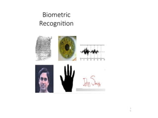
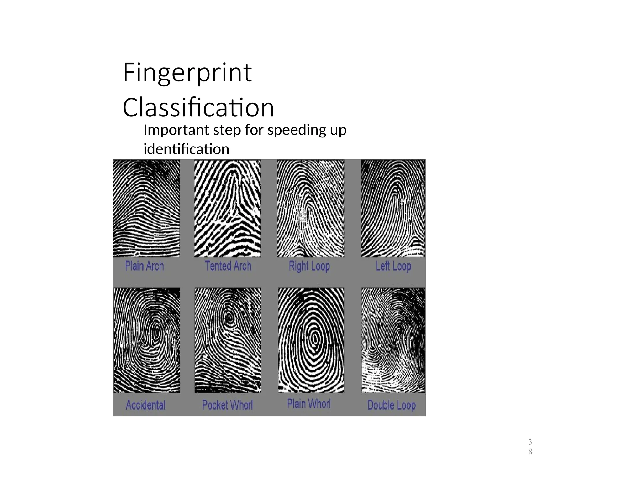
• Identification of people from
• finger prints,
• hand shape and size,
• Retinal scans
• voice characteristics,
• Typing patterns and
• handwriting
• Automatic inspection of printed circuits and printed characters
• Automatic analysis of satellite picture to determine the type and
condition of agricultural crops, weather conditions, snow and water
reserves and mineral prospects.
• Classification and analysis in medical images. : to detect a disease
3.
Features and classes
•Properties or attributes used to classify the objects are called features.
• A collection of “similar” (not necessarily same) objects are grouped together as
one “class”.
• For example:
• All the above are classified as character T
• Classes are identified by a label.
• Most of the pattern recognition tasks are first done by humans and automated later.
• Automating the classification of objects using the same features as those used by the people
can be difficult.
• Some times features that would be impossible or difficult for humans to estimate are useful in
automated system. For example satellite images use wavelengths of light that are invisible to
humans.
4.
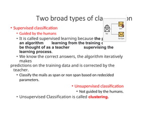
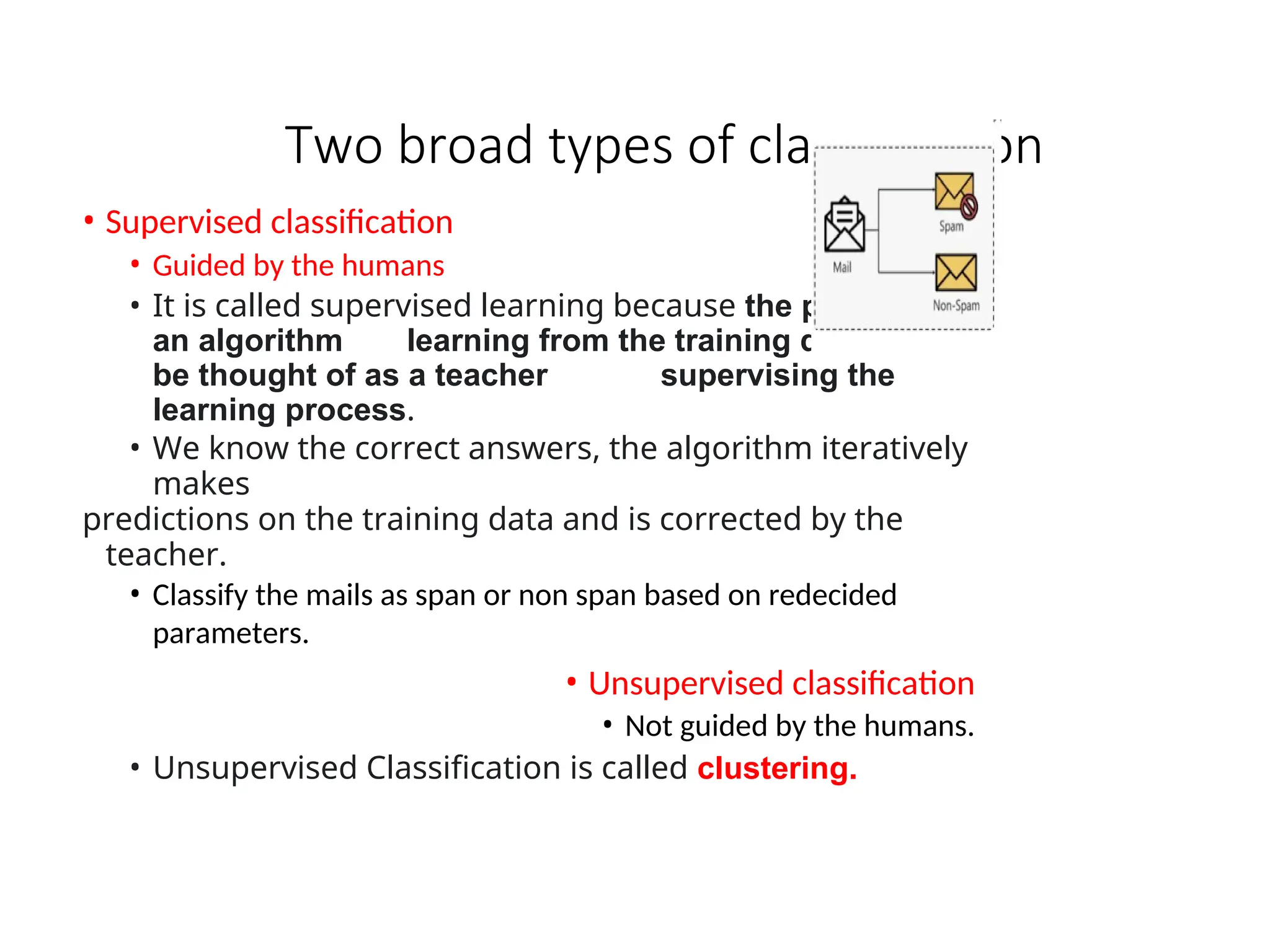
Two broad typesof classification
• Supervised classification
• Guided by the humans
• It is called supervised learning because the process of
an algorithm learning from the training dataset can
be thought of as a teacher supervising the
learning process.
• We know the correct answers, the algorithm iteratively
makes
predictions on the training data and is corrected by the
teacher.
• Classify the mails as span or non span based on redecided
parameters.
• Unsupervised classification
• Not guided by the humans.
• Unsupervised Classification is called clustering.
5.
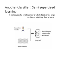
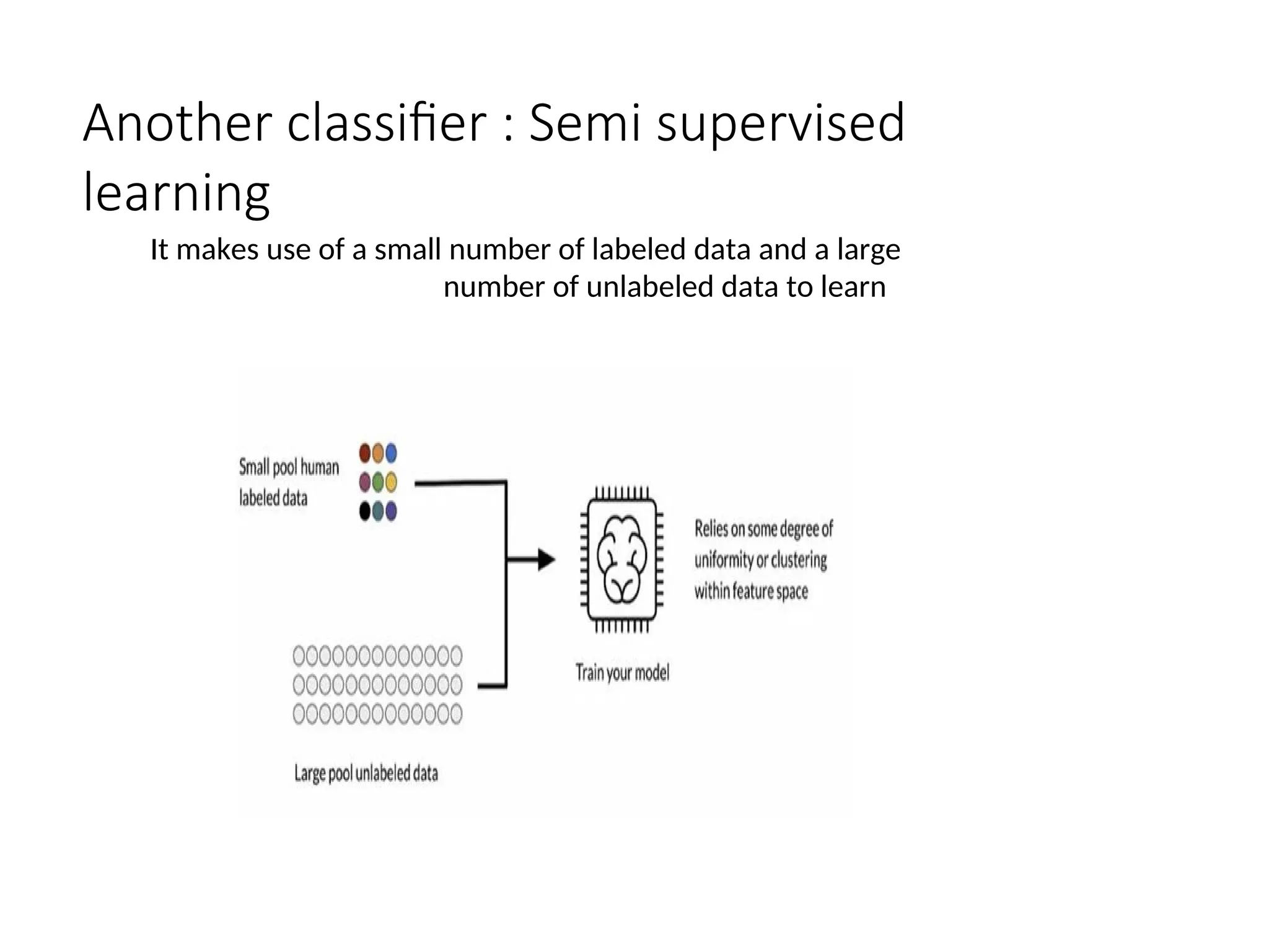
Another classifier :Semi supervised
learning
It makes use of a small number of labeled data and a large
number of unlabeled data to learn
6.
Samples or patterns
•The individual items or objects or situations to be
classified will be referred as samples or patterns or data.
• The set of data iscalled “Data Set”.
7.
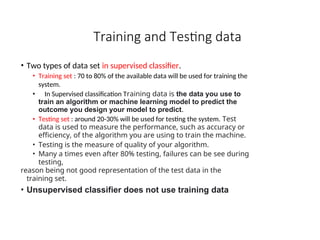
Training and Testingdata
• Two types of data set in supervised classifier.
• Training set : 70 to 80% of the available data will be used for training the
system.
• In Supervised classification Training data is the data you use to
train an algorithm or machine learning model to predict the
outcome you design your model to predict.
• Testing set : around 20-30% will be used for testing the system. Test
data is used to measure the performance, such as accuracy or
efficiency, of the algorithm you are using to train the machine.
• Testing is the measure of quality of your algorithm.
• Many a times even after 80% testing, failures can be see during
testing,
reason being not good representation of the test data in the
training set.
• Unsupervised classifier does not use training data
8.
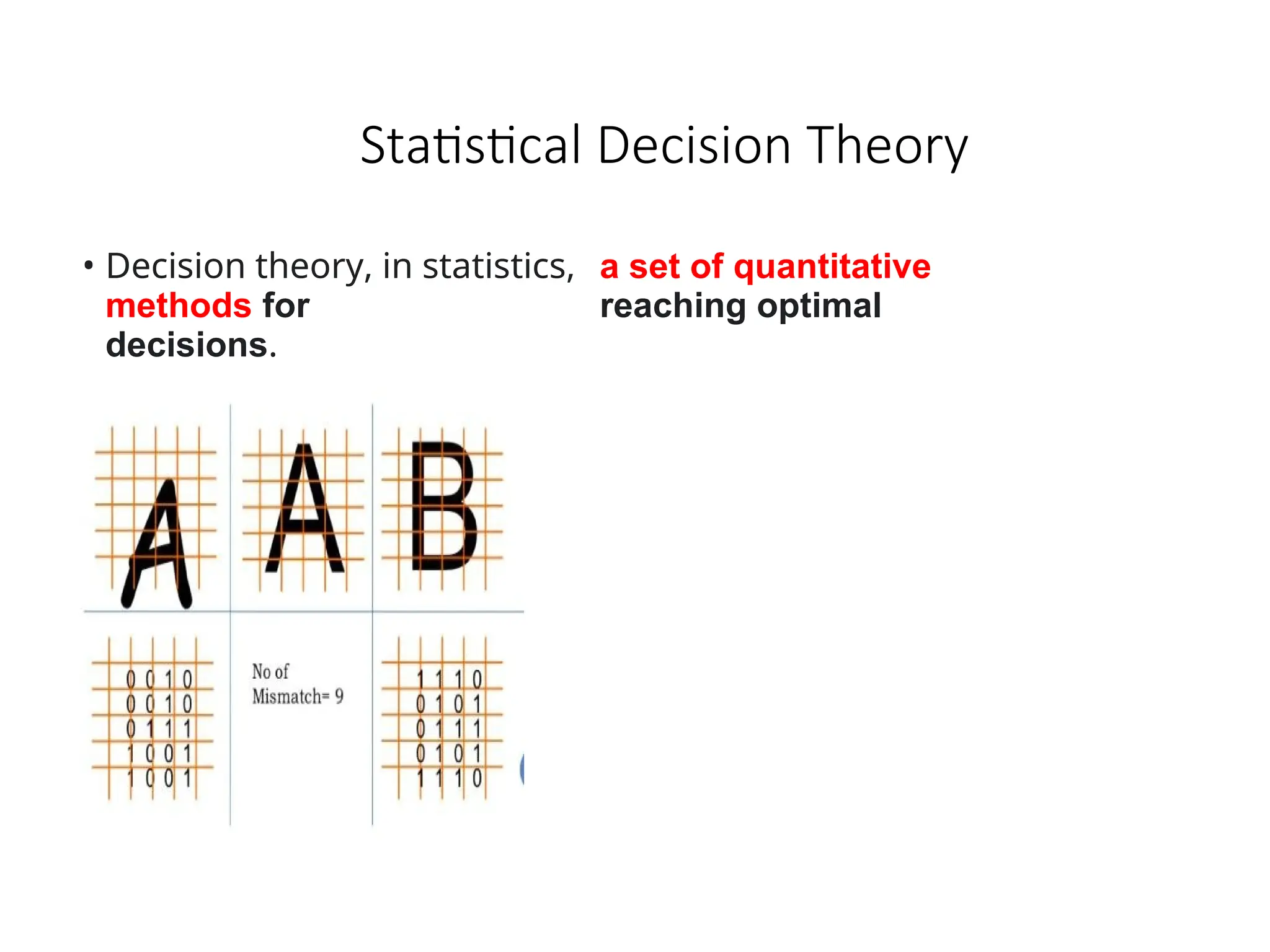
Statistical Decision Theory
•Decision theory, in statistics, a set of quantitative
methods for reaching optimal
decisions.
9.
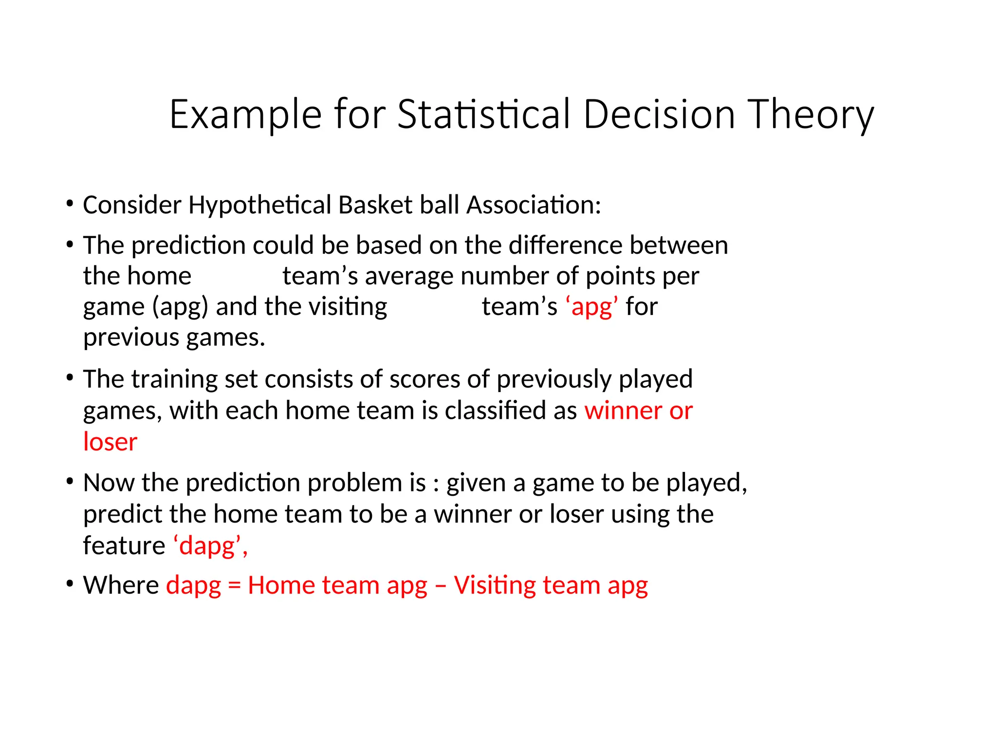
Example for StatisticalDecision Theory
• Consider Hypothetical Basket ball Association:
• The prediction could be based on the difference between
the home team’s average number of points per
game (apg) and the visiting team’s ‘apg’ for
previous games.
• The training set consists of scores of previously played
games, with each home team is classified as winner or
loser
• Now the prediction problem is : given a game to be played,
predict the home team to be a winner or loser using the
feature ‘dapg’,
• Where dapg = Home team apg – Visiting team apg
10.
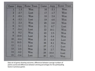
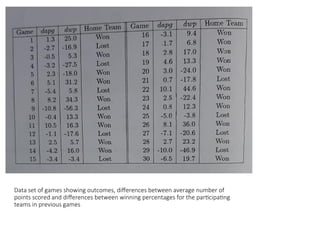
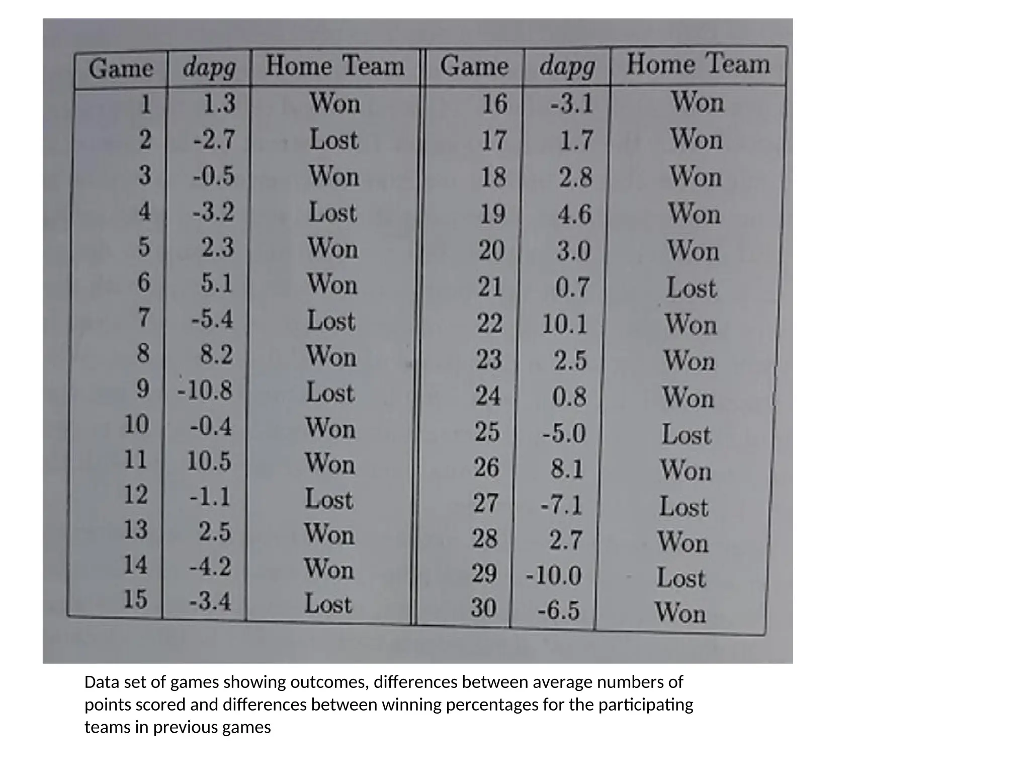
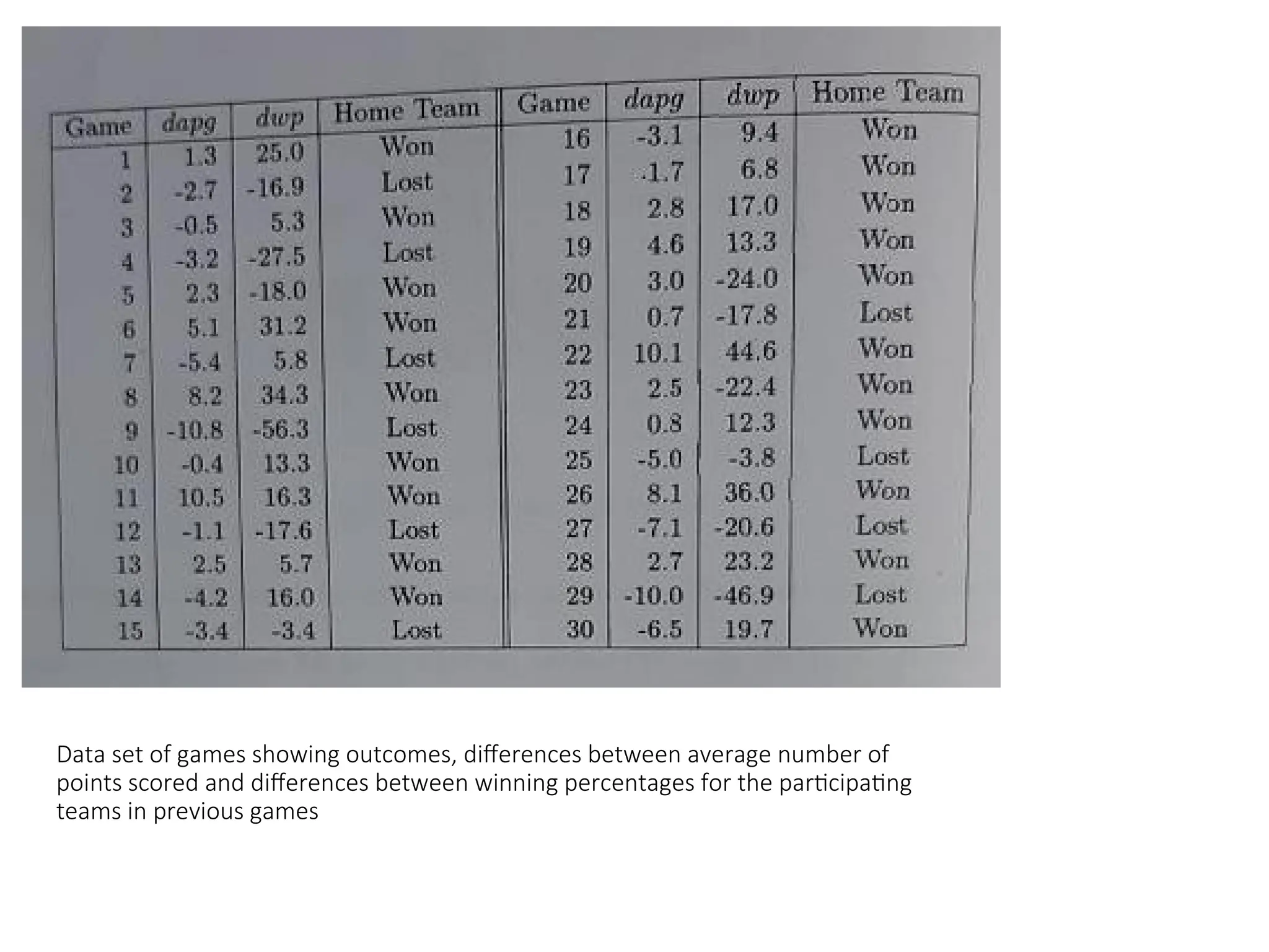
Data set ofgames showing outcomes, differences between average numbers of
points scored and differences between winning percentages for the participating
teams in previous games
11.
• The figureshown in the previous slide, lists 30 games and
gives the value of dapg for each game and tells whether the
home team won or lost.
• Notice that in this data set the team with the larger apg usually
wins.
• For example in the 9th
game the home team on average, scored 10.8 fewer points in
previous games than the visiting team, on average and also the
home team lost.
• When the teams have about the same apg’s the outcome is less
certain. For example, in the 10th game , the home team on
average scored 0.4 fewer points than the visiting team, on
average, but the home team won the match.
• Similarly 12th game, the home team had an apg 1.1. less than the
visiting team on average and the team lost.
12.
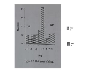
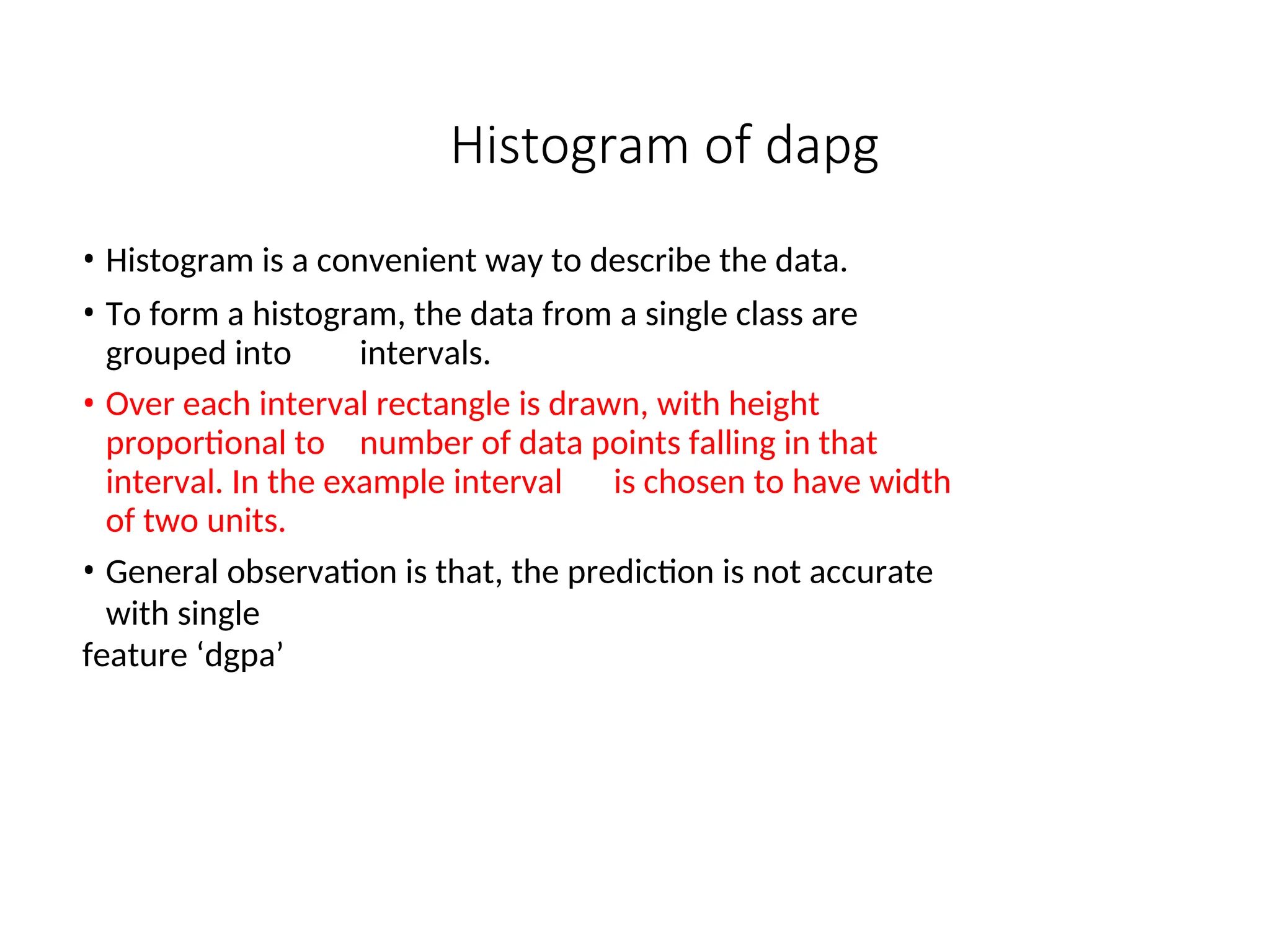
Histogram of dapg
•Histogram is a convenient way to describe the data.
• To form a histogram, the data from a single class are
grouped into intervals.
• Over each interval rectangle is drawn, with height
proportional to number of data points falling in that
interval. In the example interval is chosen to have width
of two units.
• General observation is that, the prediction is not accurate
with single
feature ‘dgpa’
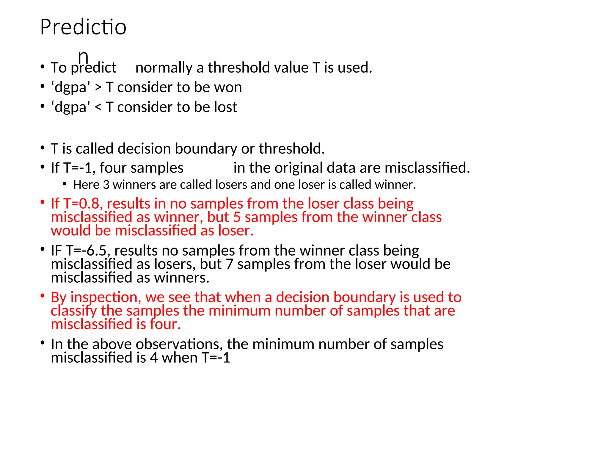
Predictio
n
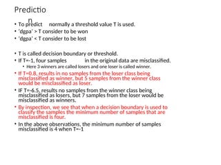
• To predictnormally a threshold value T is used.
• ‘dgpa’ > T consider to be won
• ‘dgpa’ < T consider to be lost
• T is called decision boundary or threshold.
• If T=-1, four samples in the original data are misclassified.
• Here 3 winners are called losers and one loser is called winner.
• If T=0.8, results in no samples from the loser class being
misclassified as winner, but 5 samples from the winner class
would be misclassified as loser.
• IF T=-6.5, results no samples from the winner class being
misclassified as losers, but 7 samples from the loser would be
misclassified as winners.
• By inspection, we see that when a decision boundary is used to
classify the samples the minimum number of samples that are
misclassified is four.
• In the above observations, the minimum number of samples
misclassified is 4 when T=-1
15.
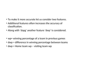
• To makeit more accurate let us consider two features.
• Additional features often increases the accuracy of
classification.
• Along with ‘dapg’ another feature ‘dwp’ is considered.
• wp= winning percentage of a team in previous games
• dwp = difference in winning percentage between teams
• dwp = Home team wp – visiting team wp
16.
Data set ofgames showing outcomes, differences between average number of
points scored and differences between winning percentages for the participating
teams in previous games
17.
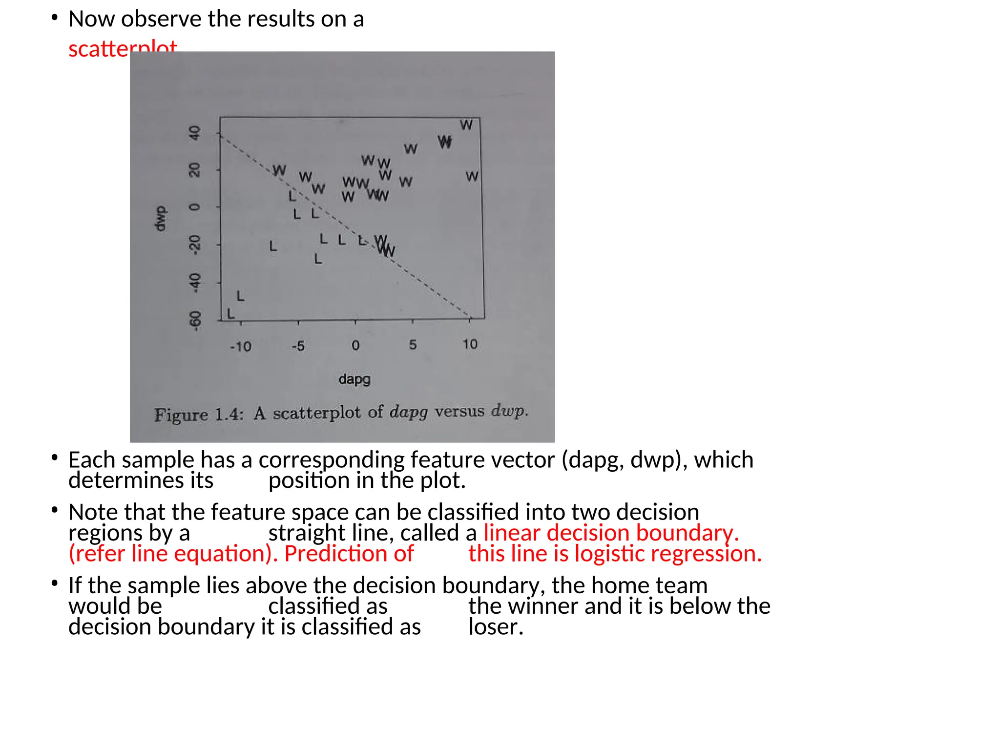
• Now observethe results on a
scatterplot
• Each sample has a corresponding feature vector (dapg, dwp), which
determines its position in the plot.
• Note that the feature space can be classified into two decision
regions by a straight line, called a linear decision boundary.
(refer line equation). Prediction of this line is logistic regression.
• If the sample lies above the decision boundary, the home team
would be classified as the winner and it is below the
decision boundary it is classified as loser.
18.
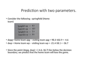
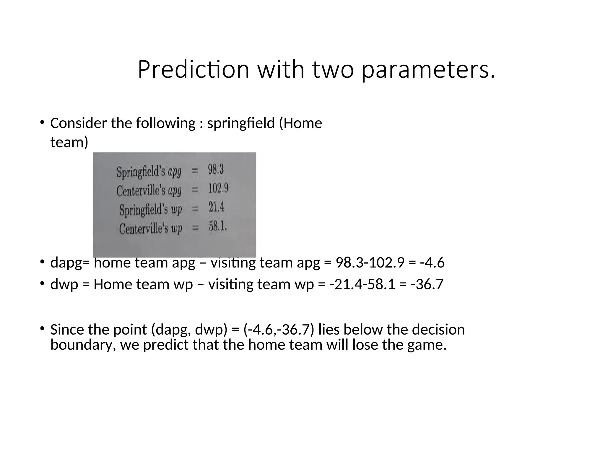
Prediction with twoparameters.
• Consider the following : springfield (Home
team)
• dapg= home team apg – visiting team apg = 98.3-102.9 = -4.6
• dwp = Home team wp – visiting team wp = -21.4-58.1 = -36.7
• Since the point (dapg, dwp) = (-4.6,-36.7) lies below the decision
boundary, we predict that the home team will lose the game.
19.
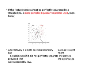
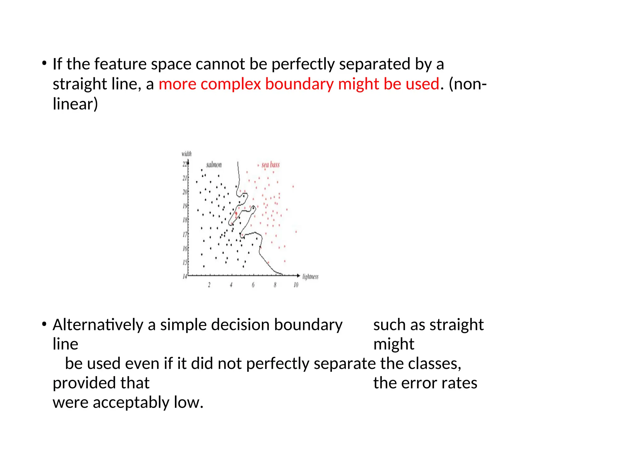
• If thefeature space cannot be perfectly separated by a
straight line, a more complex boundary might be used. (non-
linear)
• Alternatively a simple decision boundary such as straight
line might
be used even if it did not perfectly separate the classes,
provided that the error rates
were acceptably low.
20.
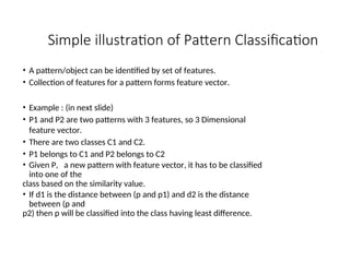
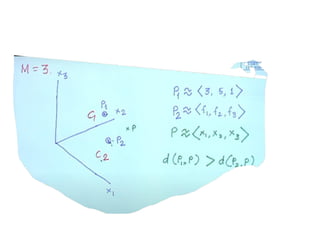
Simple illustration ofPattern Classification
• A pattern/object can be identified by set of features.
• Collection of features for a pattern forms feature vector.
• Example : (in next slide)
• P1 and P2 are two patterns with 3 features, so 3 Dimensional
feature vector.
• There are two classes C1 and C2.
• P1 belongs to C1 and P2 belongs to C2
• Given P, a new pattern with feature vector, it has to be classified
into one of the
class based on the similarity value.
• If d1 is the distance between (p and p1) and d2 is the distance
between (p and
p2) then p will be classified into the class having least difference.
22.
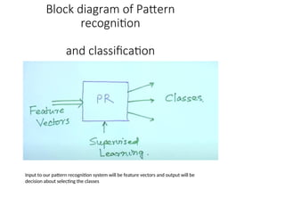
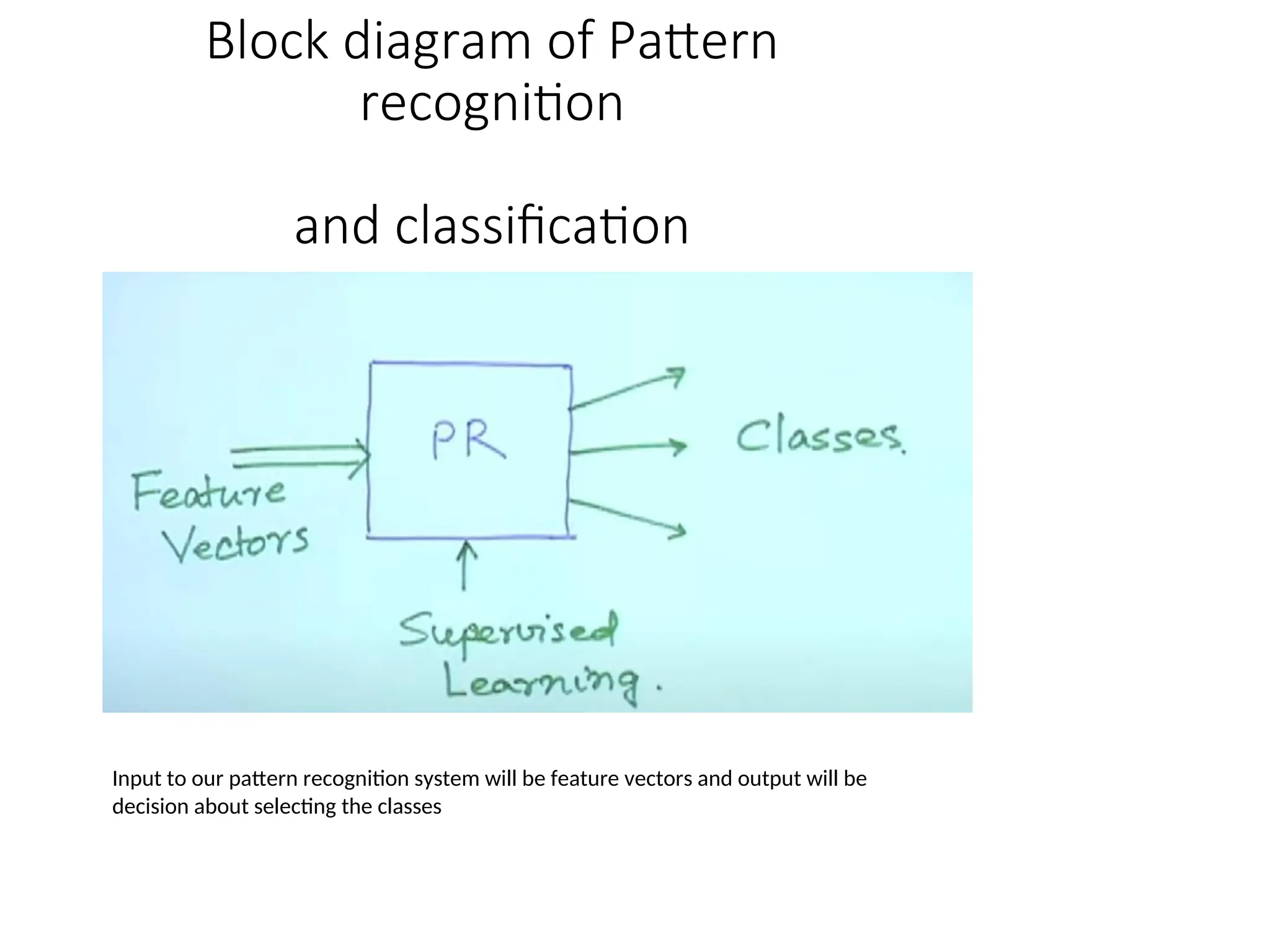
Block diagram ofPattern
recognition
and classification
Input to our pattern recognition system will be feature vectors and output will be
decision about selecting the classes
23.
• Having themodel shown in previous slide, we can use it for
any type of recognition and classification.
• It can be
• speaker recognition
• Speech recognition
• Image classification
• Video recognition and so on…
24.
• It isnow very important to learn:
• Different techniques to extract the features
• Then in the second stage, different methods to recognize
the pattern and classify
• Some of them use statistical approach
• Few uses probabilistic model using mean and variance etc.
• Other methods are - neural network, deep neural networks
• Hyper box classifier
• Fuzzy measure
• And mixture of some of the above
What is covered?
•Basics of Probability
• Combination
• Permutation
• Examples for the
above
• Union
• Intersection
• Complement
36.
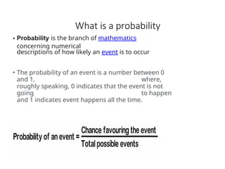
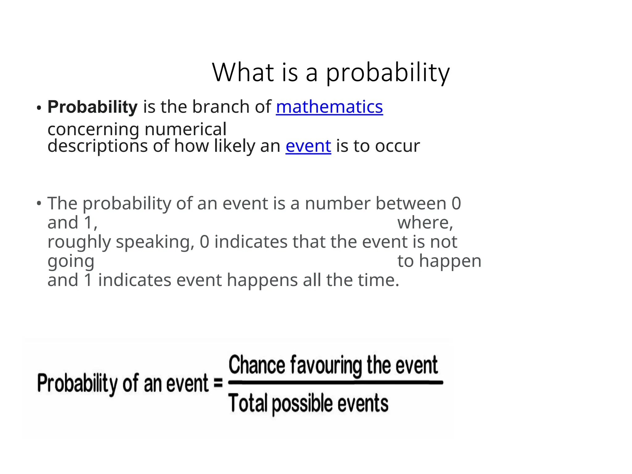
What is aprobability
• Probability is the branch of mathematics
concerning numerical
descriptions of how likely an event is to occur
• The probability of an event is a number between 0
and 1, where,
roughly speaking, 0 indicates that the event is not
going to happen
and 1 indicates event happens all the time.
37.
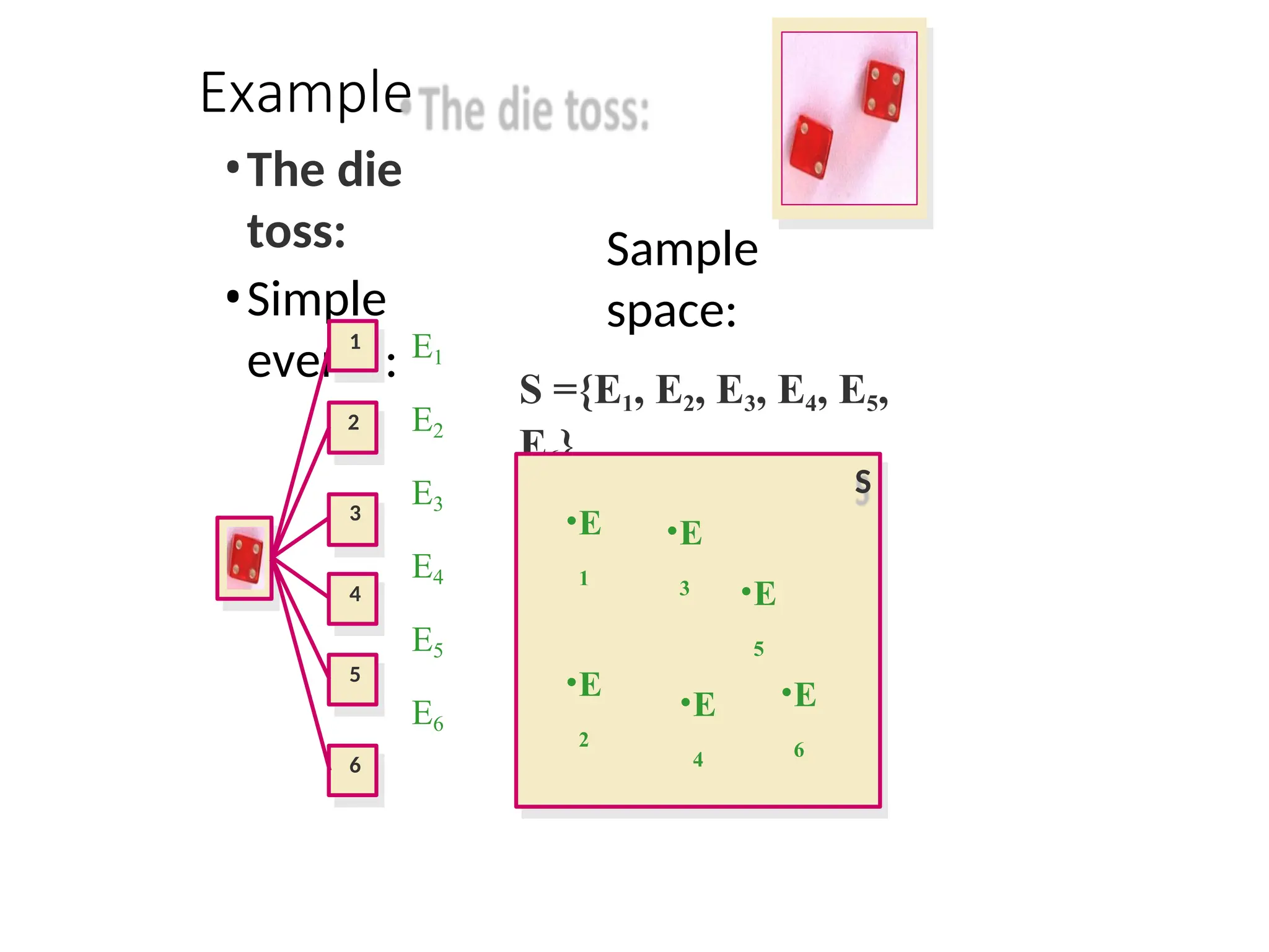
Experiment
• The termexperiment is used in probability theory to describe
a process for which the outcome is not known with
certainty.
Example of experiments are:
Rolling a fair six sided die.
Randomly choosing 5 apples from a lot of 100 apples.
38.
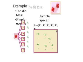
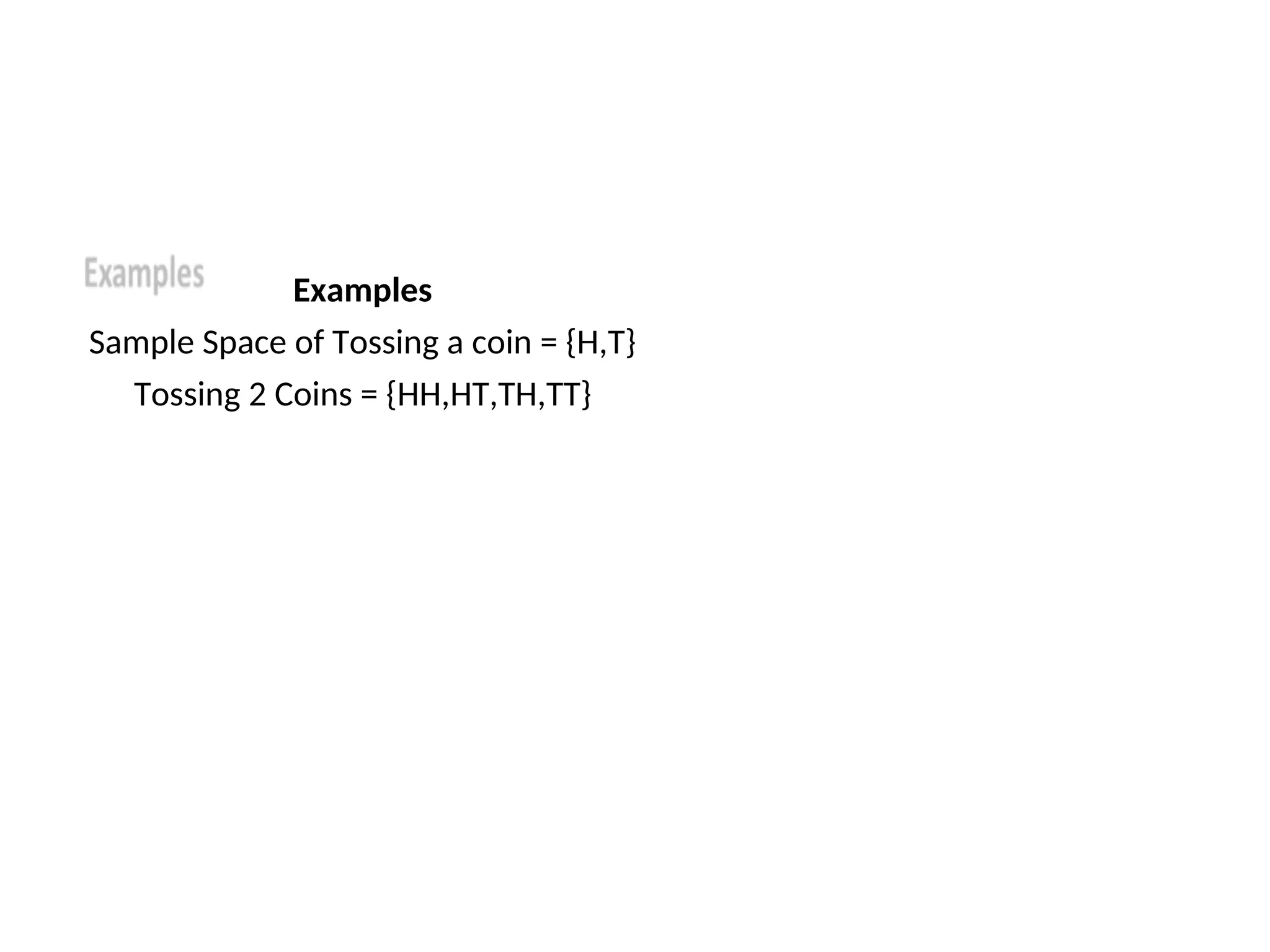
Event
• An eventis an outcome of an experiment. It is denoted
by capital
letter. Say E1,E2… or A,B….and so on
• For example toss a coin, H and T are two events.
• The event consisting of all possible outcomes of a
statistical experiment is called the “Sample Space”. Ex:
{ E1,E2…}
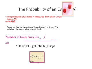
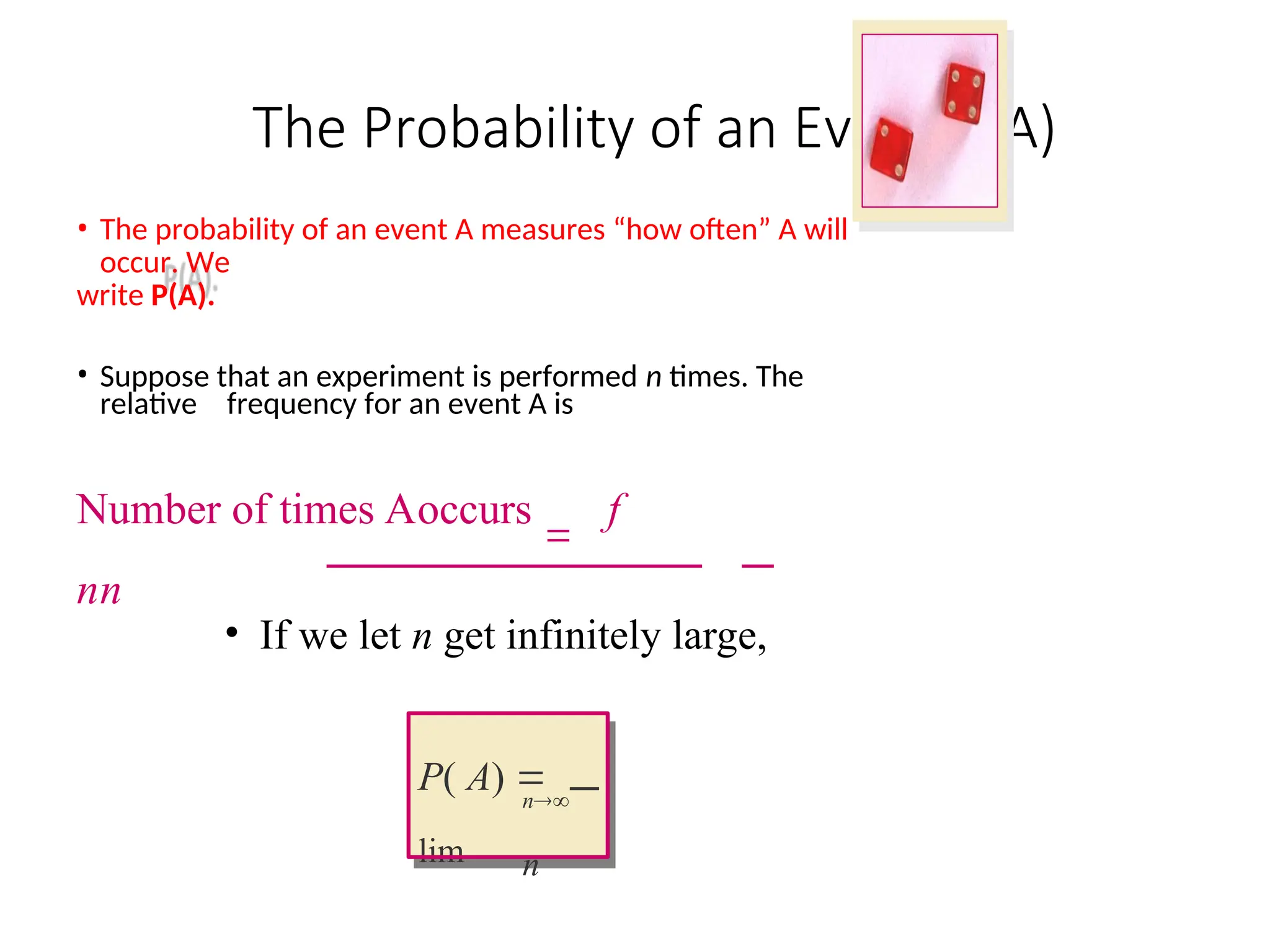
The Probability ofan Event P(A)
• The probability of an event A measures “how often” A will
occur. We
write P(A).
• Suppose that an experiment is performed n times. The
relative frequency for an event A is
Number of times Aoccurs
f
nn
• If we let n get infinitely large,
n
n
P( A)
lim
42.
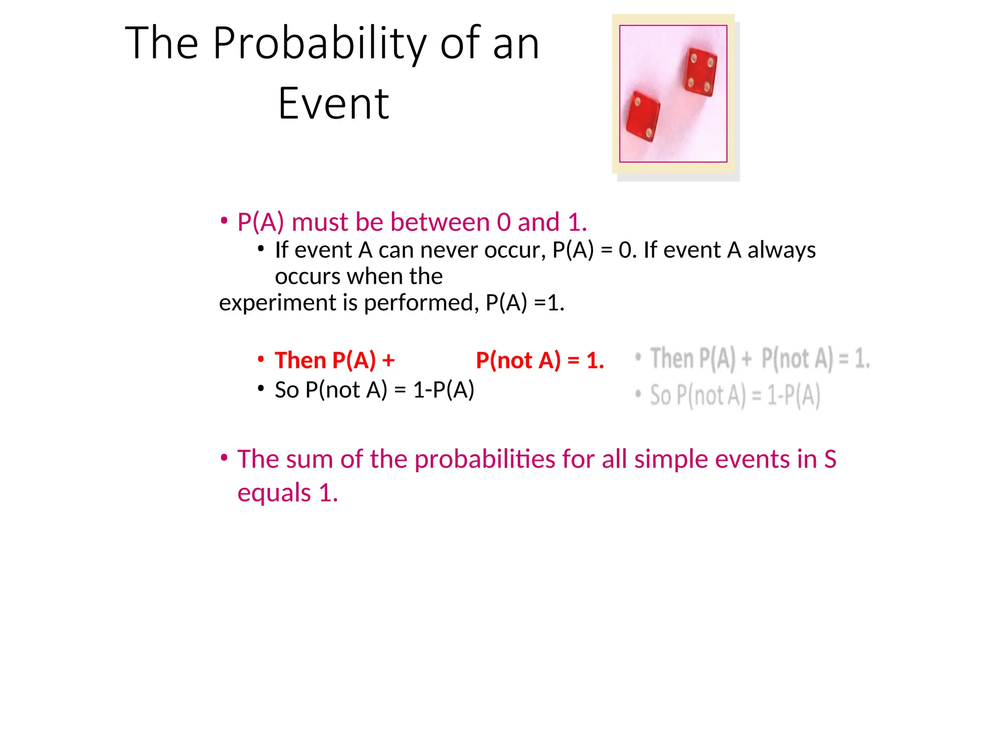
The Probability ofan
Event
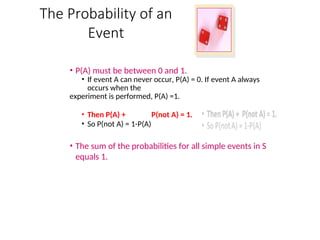
• P(A) must be between 0 and 1.
• If event A can never occur, P(A) = 0. If event A always
occurs when the
experiment is performed, P(A) =1.
• Then P(A) + P(not A) = 1.
• So P(not A) = 1-P(A)
• The sum of the probabilities for all simple events in S
equals 1.
43.
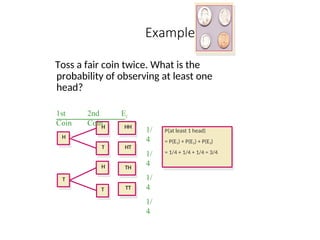
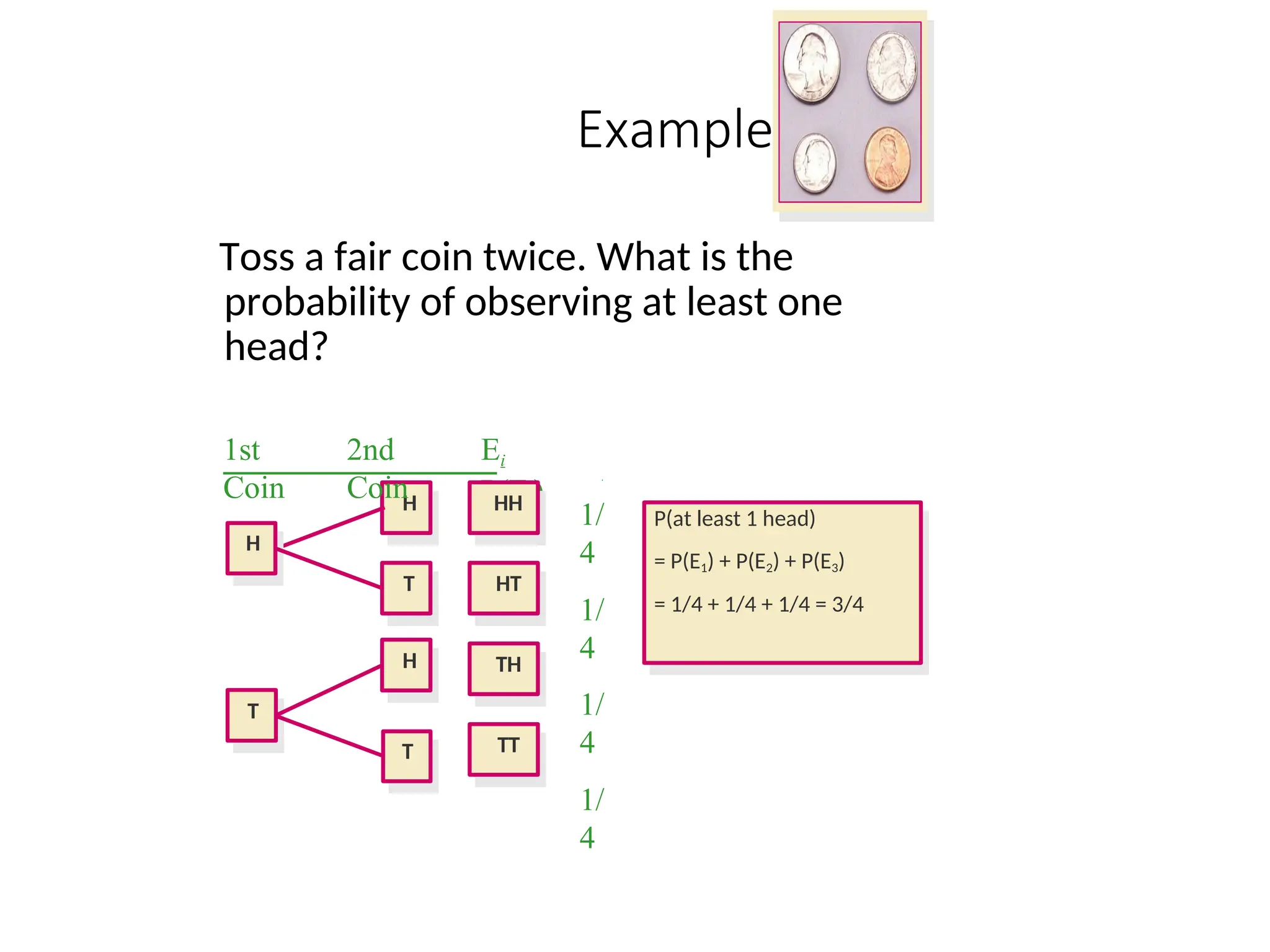
Example 1
Toss afair coin twice. What is the
probability of observing at least one
head?
H
1st
Coin
2nd
Coin
Ei
P(Ei)
H
T
T
H
T
HH
HT
TH
TT
1/
4
1/
4
1/
4
1/
4
P(at least 1 head)
= P(E1) + P(E2) + P(E3)
= 1/4 + 1/4 + 1/4 = 3/4
44.
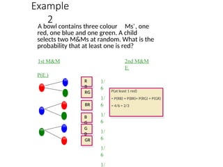
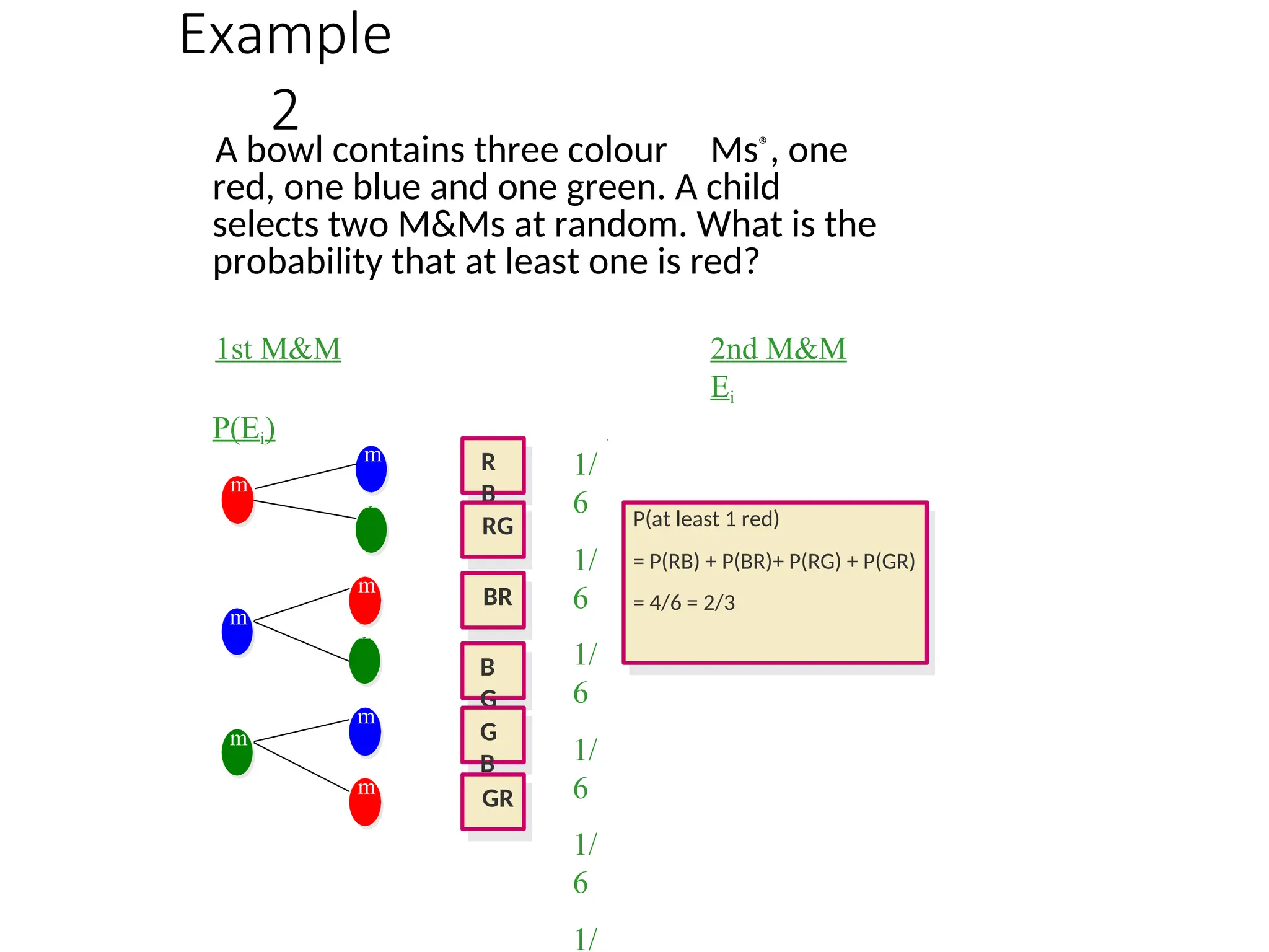
Example
2
A bowl containsthree colour Ms®, one
red, one blue and one green. A child
selects two M&Ms at random. What is the
probability that at least one is red?
1st M&M 2nd M&M
Ei
P(Ei)
R
B
RG
BR
B
G
1/
6
1/
6
1/
6
1/
6
1/
6
1/
P(at least 1 red)
= P(RB) + P(BR)+ P(RG) + P(GR)
= 4/6 = 2/3
m
m
m
m
m
m
m
m
m
G
B
GR
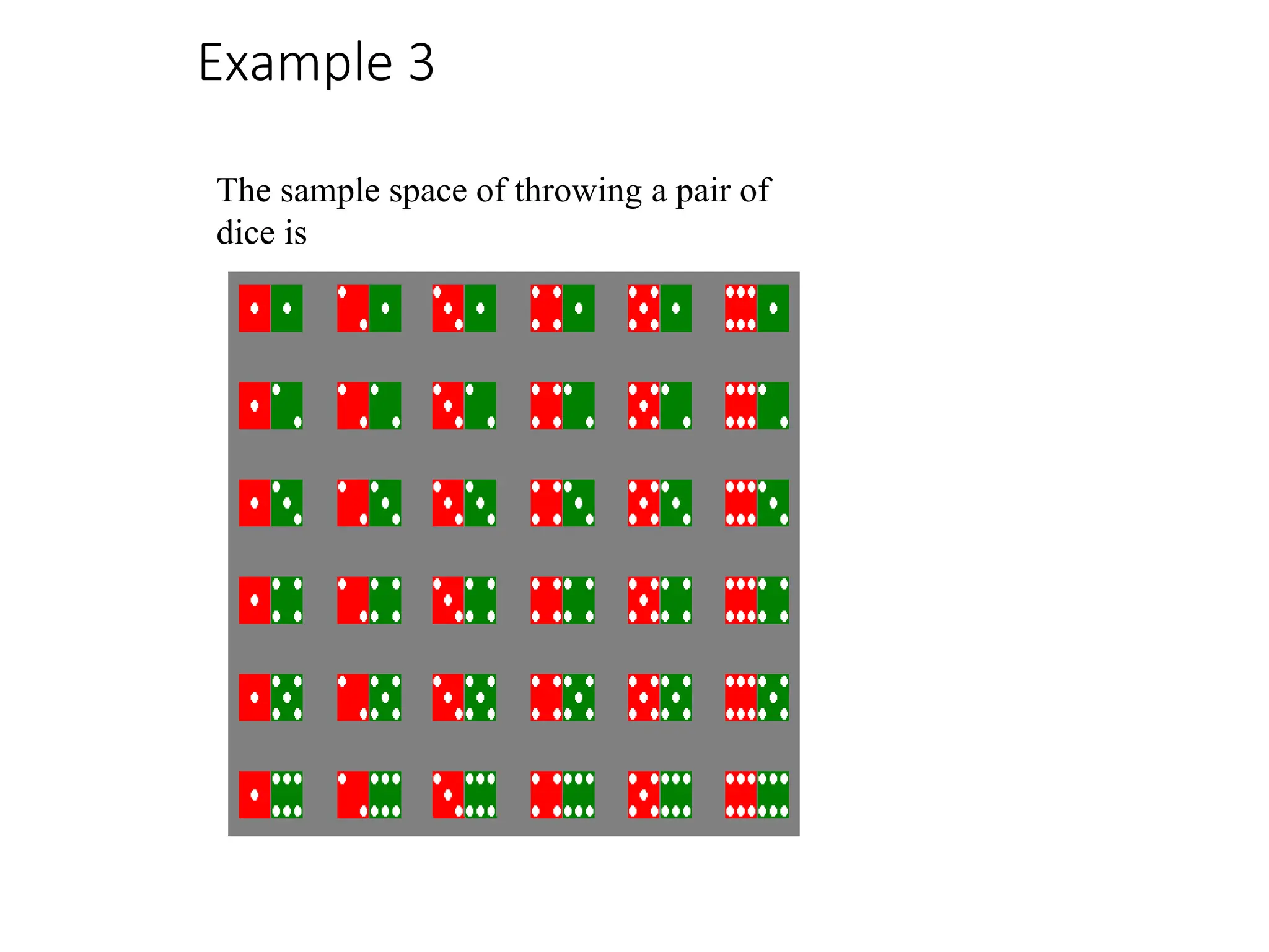
Example
3
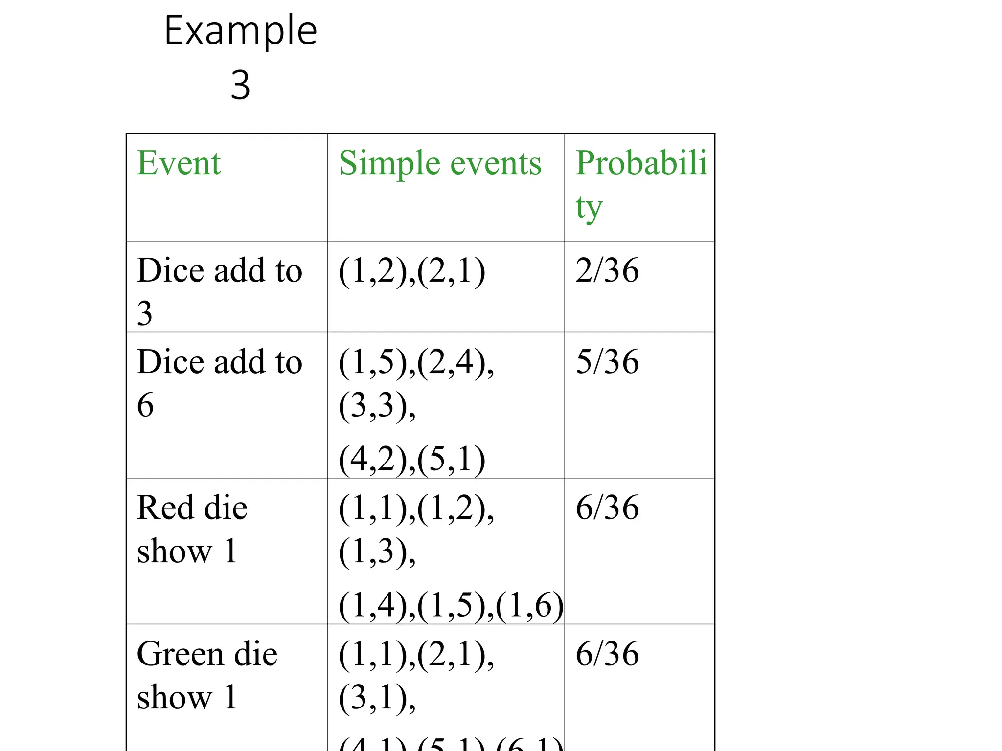
Event Simple eventsProbabili
ty
Dice add to
3
(1,2),(2,1) 2/36
Dice add to
6
(1,5),(2,4),
(3,3),
(4,2),(5,1)
5/36
Red die
show 1
(1,1),(1,2),
(1,3),
(1,4),(1,5),(1,6)
6/36
Green die
show 1
(1,1),(2,1),
(3,1),
6/36
47.
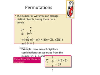
Permutations
• The numberof ways you can arrange
n distinct objects, taking them r at a
time is
where n! n(n 1)(n 2)...(2)(1)
and 0! 1.
Example: How many 3-digit lock
combinations can we make from the
numbers 1, 2, 3, and 4?
(n
r)!
n
!
Pn
r
4
!
1
!
4
3
4(3)(2)
24
P
The order of the choice is
important!
48.
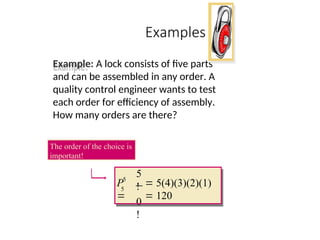
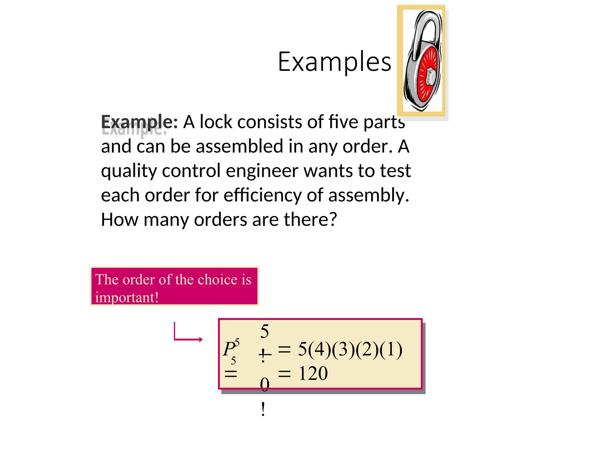
Examples
Example: A lockconsists of five parts
and can be assembled in any order. A
quality control engineer wants to test
each order for efficiency of assembly.
How many orders are there?
5
!
0
!
5
5
5(4)(3)(2)(1)
120
P
The order of the choice is
important!
49.
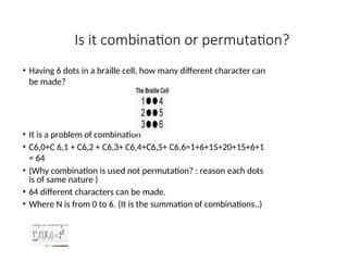
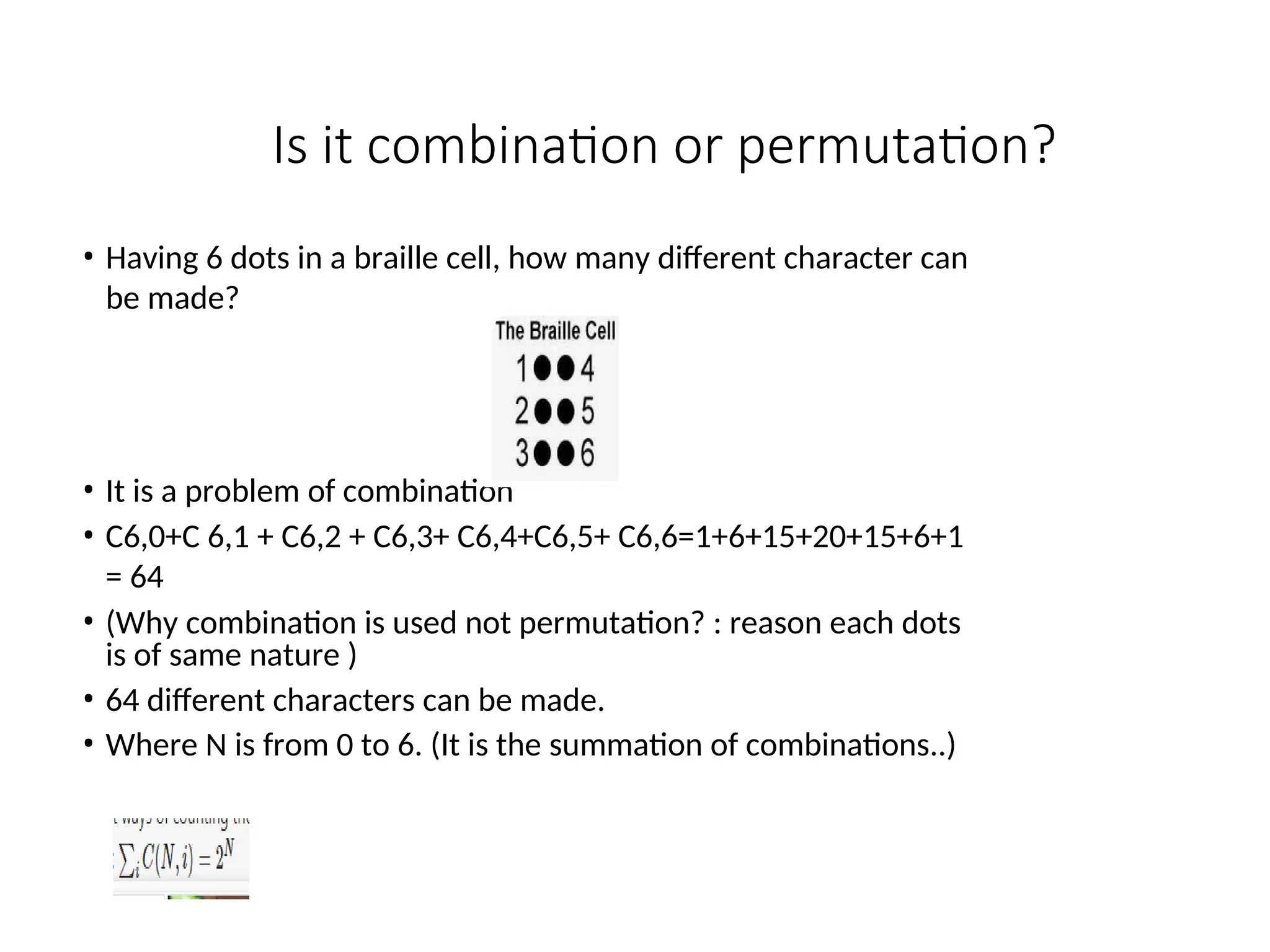
Is it combinationor permutation?
• Having 6 dots in a braille cell, how many different character can
be made?
• It is a problem of combination
• C6,0+C 6,1 + C6,2 + C6,3+ C6,4+C6,5+ C6,6=1+6+15+20+15+6+1
= 64
• (Why combination is used not permutation? : reason each dots
is of same nature )
• 64 different characters can be made.
• Where N is from 0 to 6. (It is the summation of combinations..)
50.
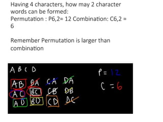
Having 4 characters,how may 2 character
words can be formed:
Permutation : P6,2= 12 Combination: C6,2 =
6
Remember Permutation is larger than
combination
51.
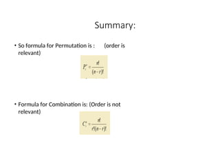
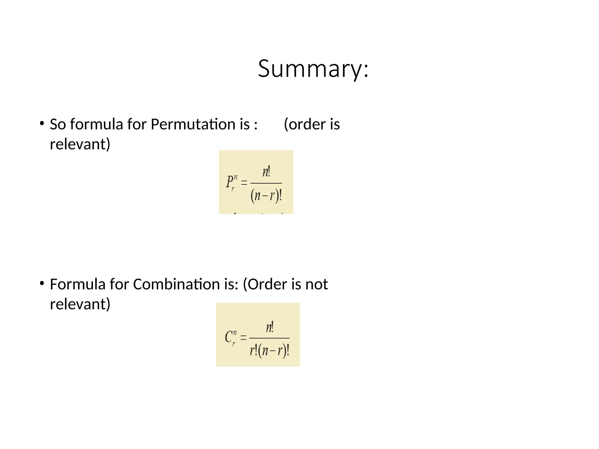
Summary:
• So formulafor Permutation is : (order is
relevant)
• Formula for Combination is: (Order is not
relevant)
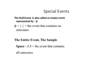
Special Events
The NullEvent, is also called as empty event
represented by -
= { } = the event that contains no
outcomes
The Entire Event, The Sample
Space - S S = the event that contains
all outcomes
54.
3 Basic Event
relations
1.Union if you see the word or,
2. Intersection if you see the
word and,
3. Complement if you see the
word not.
55.
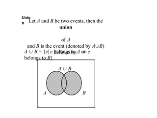
Unio
n Let Aand B be two events, then the
union
of A
and B is the event (denoted by AB)
defined by:
A B = {e| e belongs to A or e
belongs to B}
A B
A B
56.
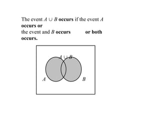
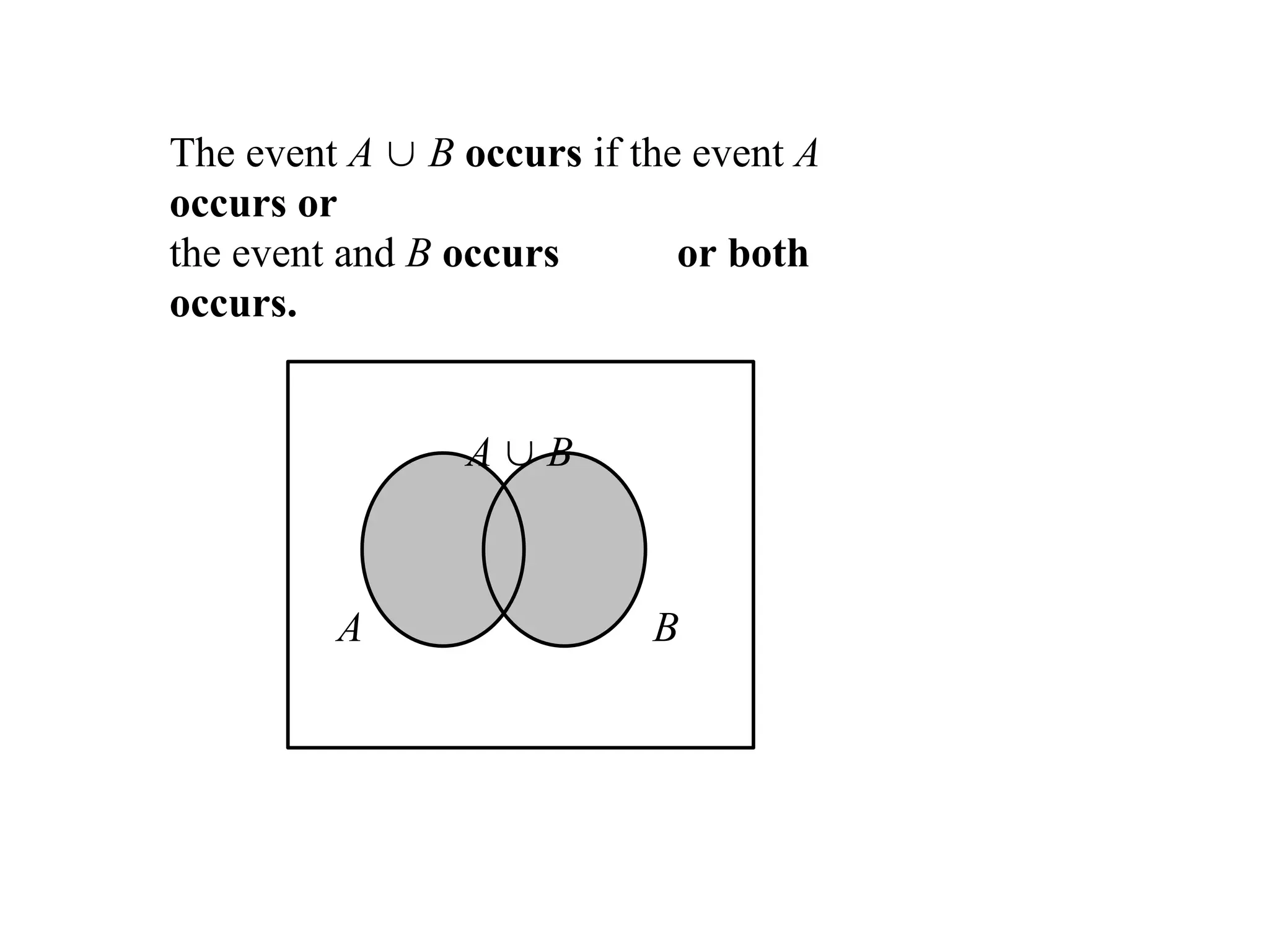
The event A B occurs if the event A
occurs or
the event and B occurs or both
occurs.
A B
A B
57.
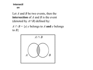
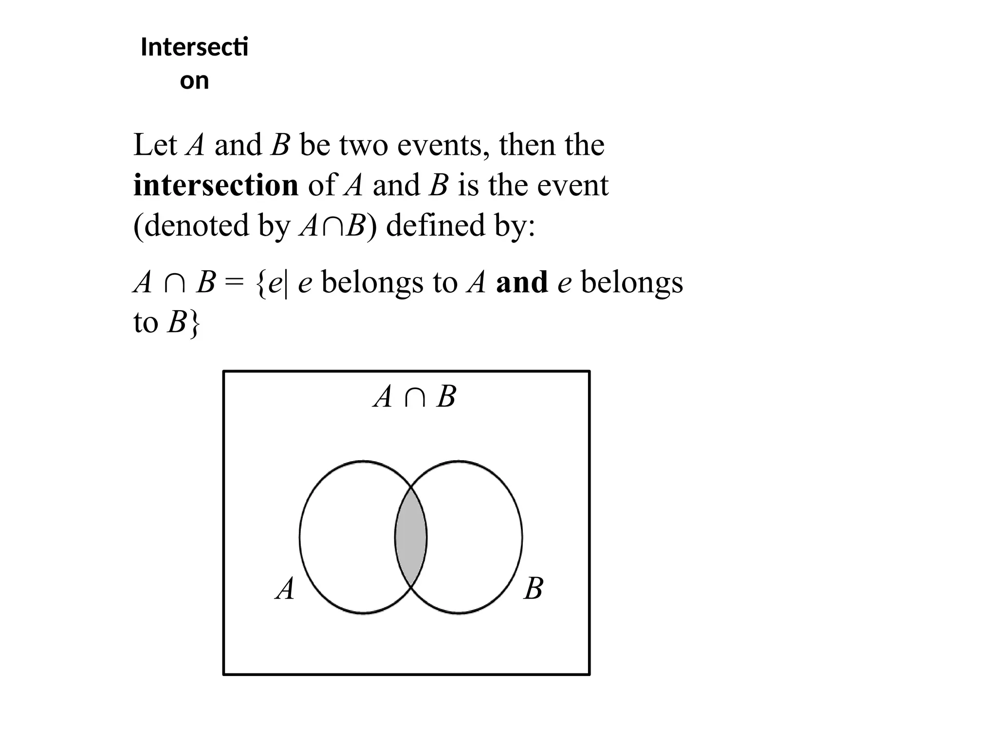
Intersecti
on
Let A andB be two events, then the
intersection of A and B is the event
(denoted by AB) defined by:
A B = {e| e belongs to A and e belongs
to B}
A B
A B
58.
A B
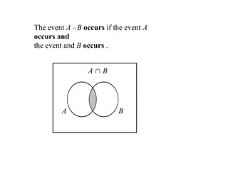
The eventA B occurs if the event A
occurs and
the event and B occurs .
A B
59.
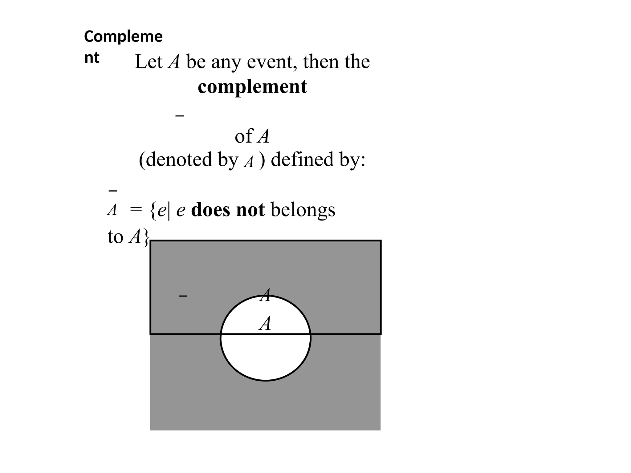
Compleme
nt
A = {e|e does not belongs
to A}
Let A be any event, then the
complement
of A
(denoted by A ) defined by:
A
A
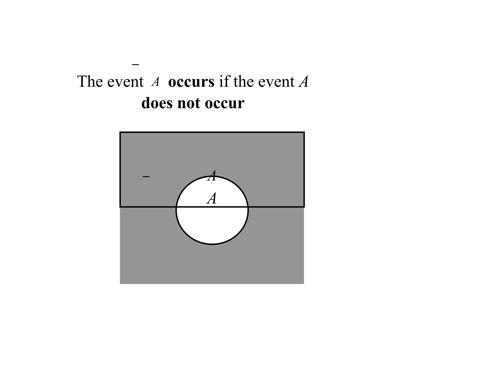
60.
The event Aoccurs if the event A
does not occur
A
A
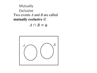
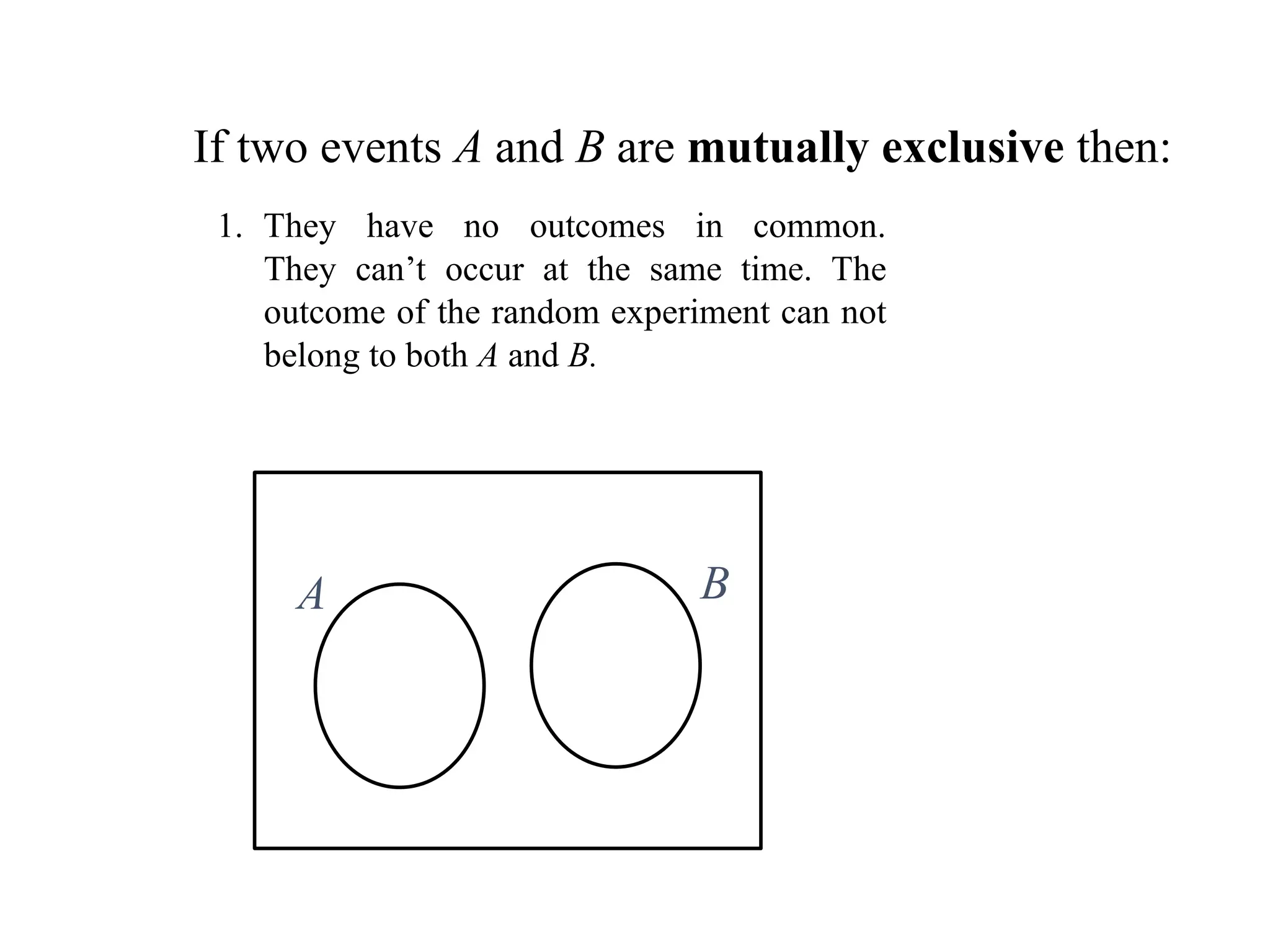
If two eventsA and B are mutually exclusive then:
A B
1. They have no outcomes in common.
They can’t occur at the same time. The
outcome of the random experiment can not
belong to both A and B.
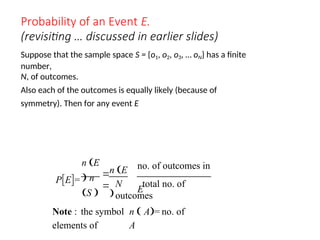
Probability of anEvent E.
(revisiting … discussed in earlier slides)
Suppose that the sample space S = {o1, o2, o3, … oN} has a finite
number,
N, of outcomes.
Also each of the outcomes is equally likely (because of
symmetry). Then for any event E
PE=
n E
n
S
n E
no. of outcomes in
E
N total no. of
outcomes
Note : the symbol n A= no. of
elements of A
The additive rule(Mutually exclusive events) if A
B =
P[A B] = P[A] +
P[B]
i.e.
P[A or B] = P[A] +
P[B]
if A B =
(A and B mutually
exclusive)
67.
Logi
c
A
B
B
A
A
B
WhenP[A] is added to P[B] the outcome in A B are
counted twice
hence
P[A B] = P[A] + P[B] – P[A B]
68.
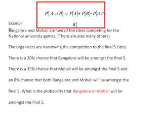
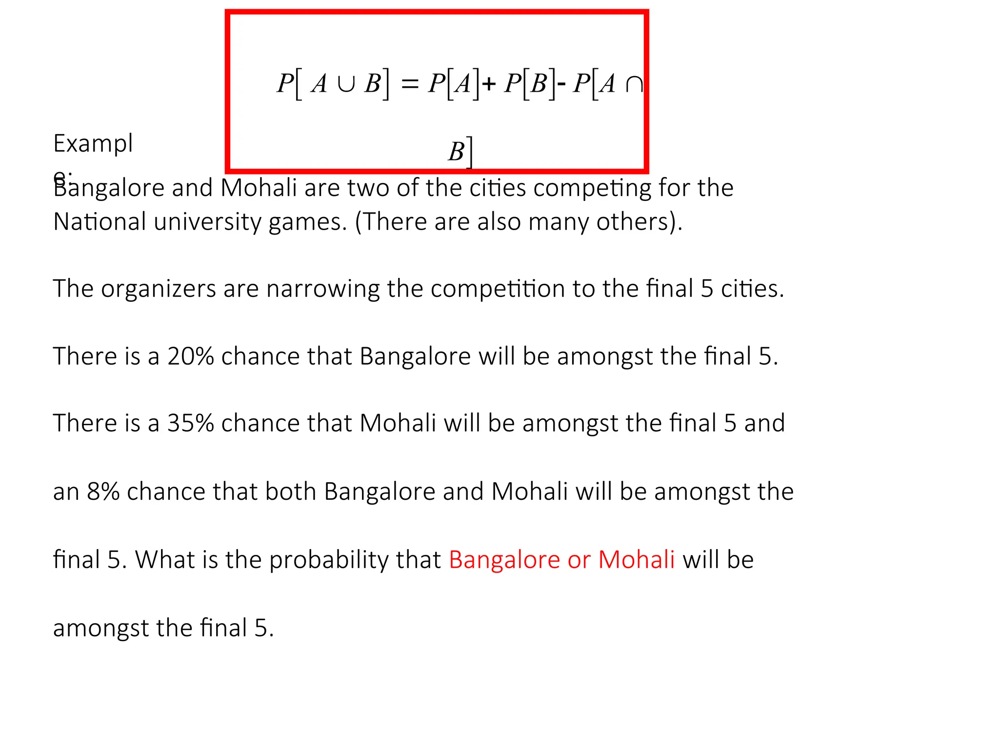
P A B PA PB PA
B
Exampl
e:
Bangalore and Mohali are two of the cities competing for the
National university games. (There are also many others).
The organizers are narrowing the competition to the final 5 cities.
There is a 20% chance that Bangalore will be amongst the final 5.
There is a 35% chance that Mohali will be amongst the final 5 and
an 8% chance that both Bangalore and Mohali will be amongst the
final 5. What is the probability that Bangalore or Mohali will be
amongst the final 5.
69.
Solution:
Let A =the event that Bangalore is amongst the
final 5. Let B = the event that Mohali is amongst
the final 5.
Given P[A] = 0.20, P[B] = 0.35, and P[A B]
= 0.08
What is P[A B]?
Note: “and” ≡ , “or” ≡ .
P A B PA PB PA B
0.20 0.35 0.08 0.47
70.
Find the probabilityof drawing an ace or a spade from a deck
of cards.
There are 52 cards in a deck; 13 are spades, 4 are aces.
Probability of a single card being spade is:
13/52 Probability of drawing an Ace is :
4/52
= 1/4.
=
1/13.
Probability of a single card being both Spade and Ace
= 1/52.
Let A = Event of drawing a spade . Let B = Event
drawing Ace.
Given P[A] =1/4, P[B] =1/13, and P[A B] = 1/52
P A B PA PB PA B
P[A B] = 1/4 + 1/13 – 1/52
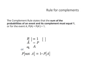
Rule for complements
𝑃
𝐴
ሜ
=1
− 𝑃
𝐴
or
Pnot A 1 PA
The Complement Rule states that the sum of the
probabilities of an event and its complement must equal 1,
or for the event A, P(A) + P(A') = 1.
73.
Compleme
nt
A = {e|e does not belongs
to A}
Let A be any event, then the
complement
of A
(denoted by A ) defined by:
A
A
74.
The event Aoccurs if the event A
does not occur
A
A
75.
A
A
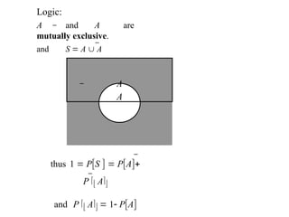
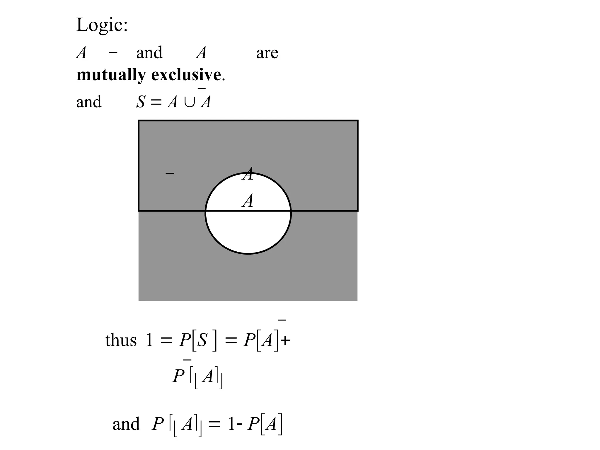
Logic:
A and Aare
mutually exclusive.
and S A A
thus 1 PS PA
P A
and P A 1 PA
76.
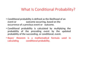
What Is ConditionalProbability?
• Conditional probability is defined as the likelihood of an
event or outcome occurring, based on the
occurrence of a previous event or outcome.
• Conditional probability is calculated by multiplying the
probability of the preceding event by the updated
probability of the succeeding, or conditional, event.
• Bayes' theorem is a mathematical formula used in
calculating conditional probability.
77.
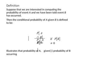
Definition
Suppose that weare interested in computing the
probability of event A and we have been told event B
has occurred.
Then the conditional probability of A given B is defined
to be:
PB
P A
B
P A
B
if PB
0
Illustrates that probability of A, given(|) probability of B
occurring
78.
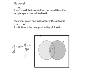
Rational
e:
PB
P AB
P A
B
B
If we’re told that event B has occurred then the
sample space is restricted to B.
The event A can now only occur if the outcome
is in of
A ∩ B. Hence the new probability of A in Bis:
A
A ∩
B
79.
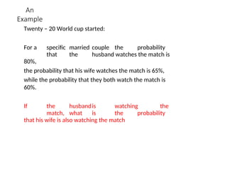
An
Example
Twenty – 20World cup started:
For a specific married couple the probability
that the husband watches the match is
80%,
the probability that his wife watches the match is 65%,
while the probability that they both watch the match is
60%.
If the husbandis watching the
match, what is the probability
that his wife is also watching the match
80.
Solutio
n:
Let B =the event that the husband watches the
match
P[B]= 0.80
Let A = the event that his wife watches the
match
P[A]= 0.65 and
P[A ∩ B]= 0.60
PB
P A
B
P A
B
0.8
0
0.60
0.75
81.
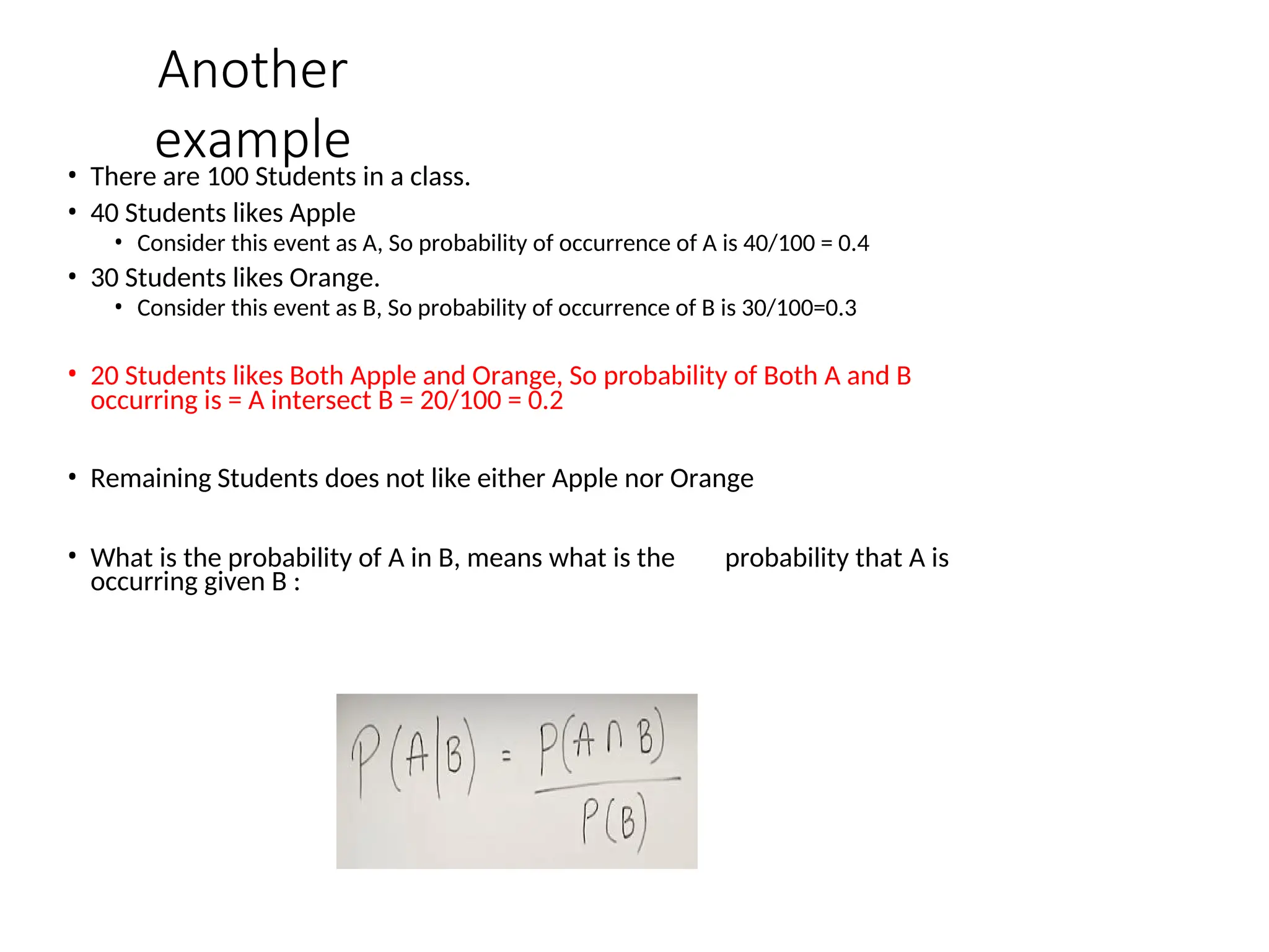
Another
example
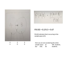
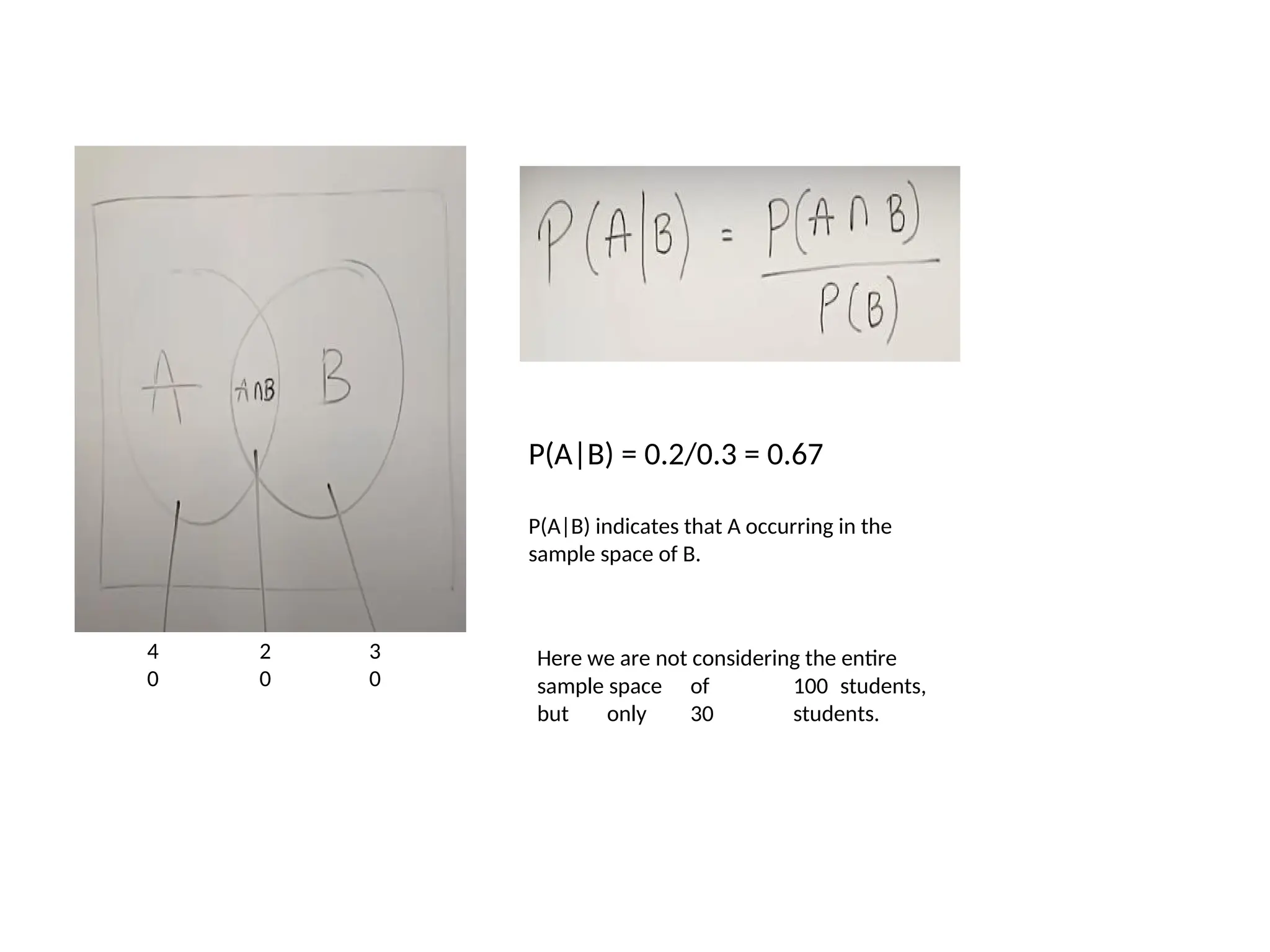
• There are100 Students in a class.
• 40 Students likes Apple
• Consider this event as A, So probability of occurrence of A is 40/100 = 0.4
• 30 Students likes Orange.
• Consider this event as B, So probability of occurrence of B is 30/100=0.3
• 20 Students likes Both Apple and Orange, So probability of Both A and B
occurring is = A intersect B = 20/100 = 0.2
• Remaining Students does not like either Apple nor Orange
• What is the probability of A in B, means what is the probability that A is
occurring given B :
82.
4
0
2
0
3
0
P(A|B) = 0.2/0.3= 0.67
P(A|B) indicates that A occurring in the
sample space of B.
Here we are not considering the entire
sample space of 100 students,
but only 30 students.
83.
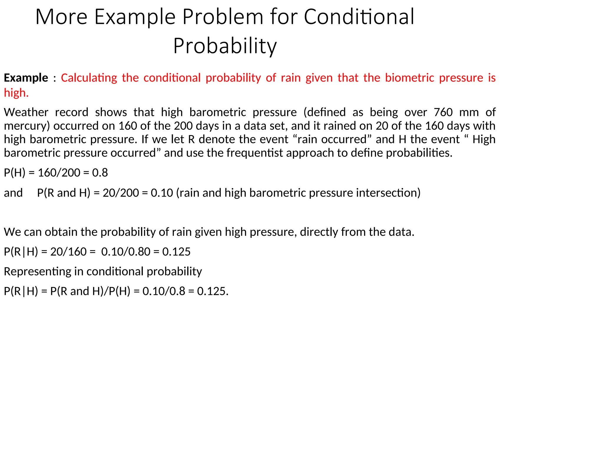
More Example Problemfor Conditional
Probability
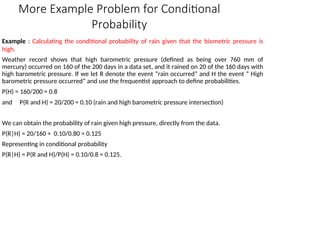
Example : Calculating the conditional probability of rain given that the biometric pressure is
high.
Weather record shows that high barometric pressure (defined as being over 760 mm of
mercury) occurred on 160 of the 200 days in a data set, and it rained on 20 of the 160 days with
high barometric pressure. If we let R denote the event “rain occurred” and H the event “ High
barometric pressure occurred” and use the frequentist approach to define probabilities.
P(H) = 160/200 = 0.8
and P(R and H) = 20/200 = 0.10 (rain and high barometric pressure intersection)
We can obtain the probability of rain given high pressure, directly from the data.
P(R|H) = 20/160 = 0.10/0.80 = 0.125
Representing in conditional probability
P(R|H) = P(R and H)/P(H) = 0.10/0.8 = 0.125.
84.
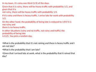
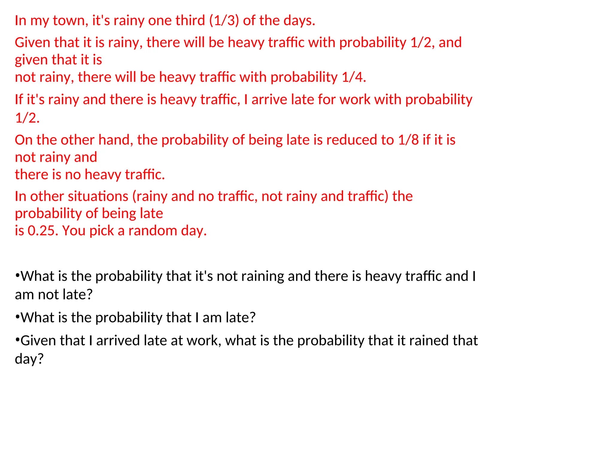
In my town,it's rainy one third (1/3) of the days.
Given that it is rainy, there will be heavy traffic with probability 1/2, and
given that it is
not rainy, there will be heavy traffic with probability 1/4.
If it's rainy and there is heavy traffic, I arrive late for work with probability
1/2.
On the other hand, the probability of being late is reduced to 1/8 if it is
not rainy and
there is no heavy traffic.
In other situations (rainy and no traffic, not rainy and traffic) the
probability of being late
is 0.25. You pick a random day.
•What is the probability that it's not raining and there is heavy traffic and I
am not late?
•What is the probability that I am late?
•Given that I arrived late at work, what is the probability that it rained that
day?
86.
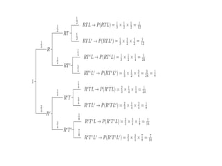
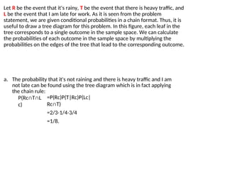
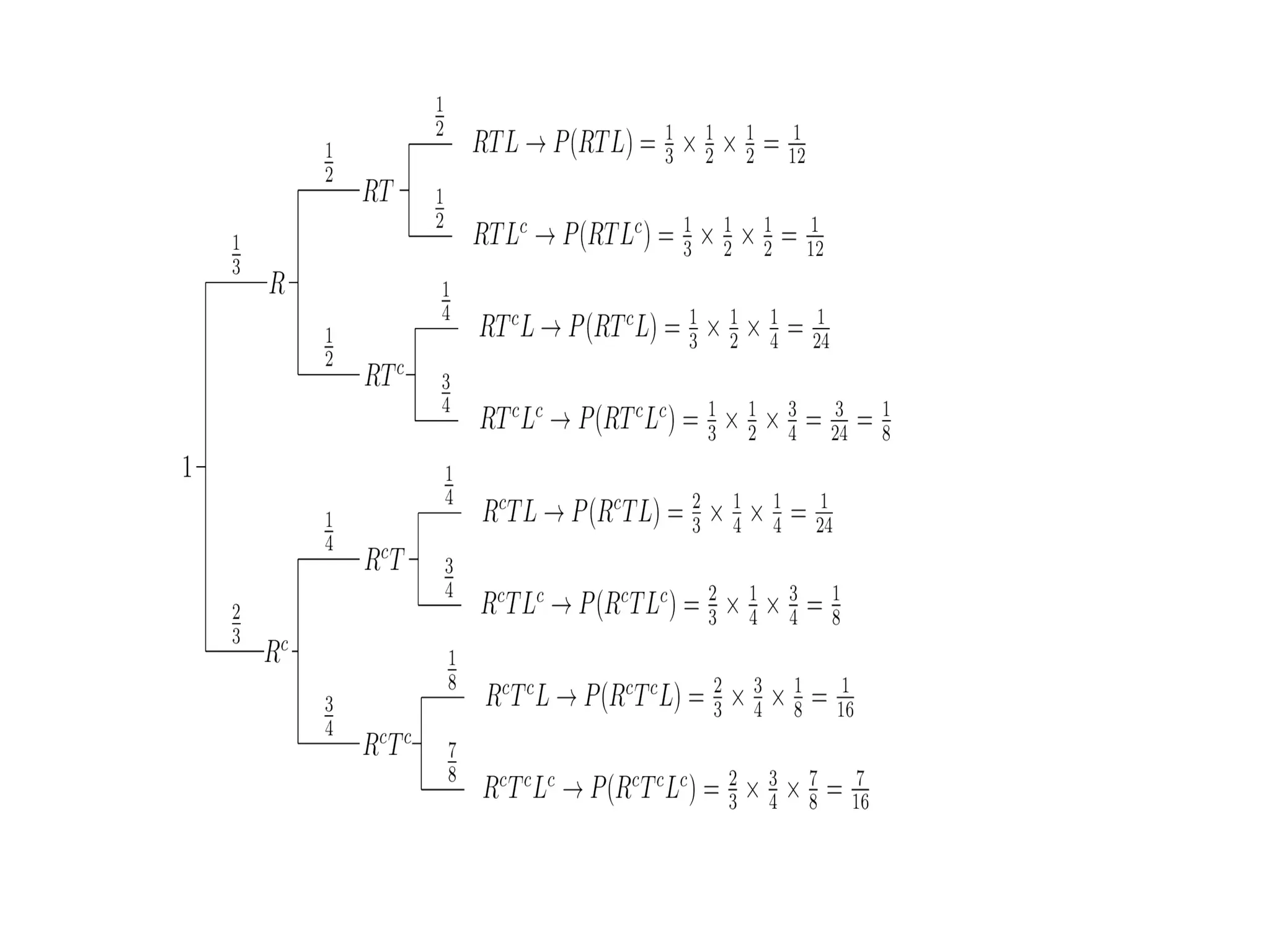
Let R bethe event that it's rainy, T be the event that there is heavy traffic, and
L be the event that I am late for work. As it is seen from the problem
statement, we are given conditional probabilities in a chain format. Thus, it is
useful to draw a tree diagram for this problem. In this figure, each leaf in the
tree corresponds to a single outcome in the sample space. We can calculate
the probabilities of each outcome in the sample space by multiplying the
probabilities on the edges of the tree that lead to the corresponding outcome.
a. The probability that it's not raining and there is heavy traffic and I am
not late can be found using the tree diagram which is in fact applying
the chain rule:
P(Rc∩T∩L
c)
=P(Rc)P(T|Rc)P(Lc|
Rc∩T)
=2/3⋅1/4⋅3/4
=1/8.
87.
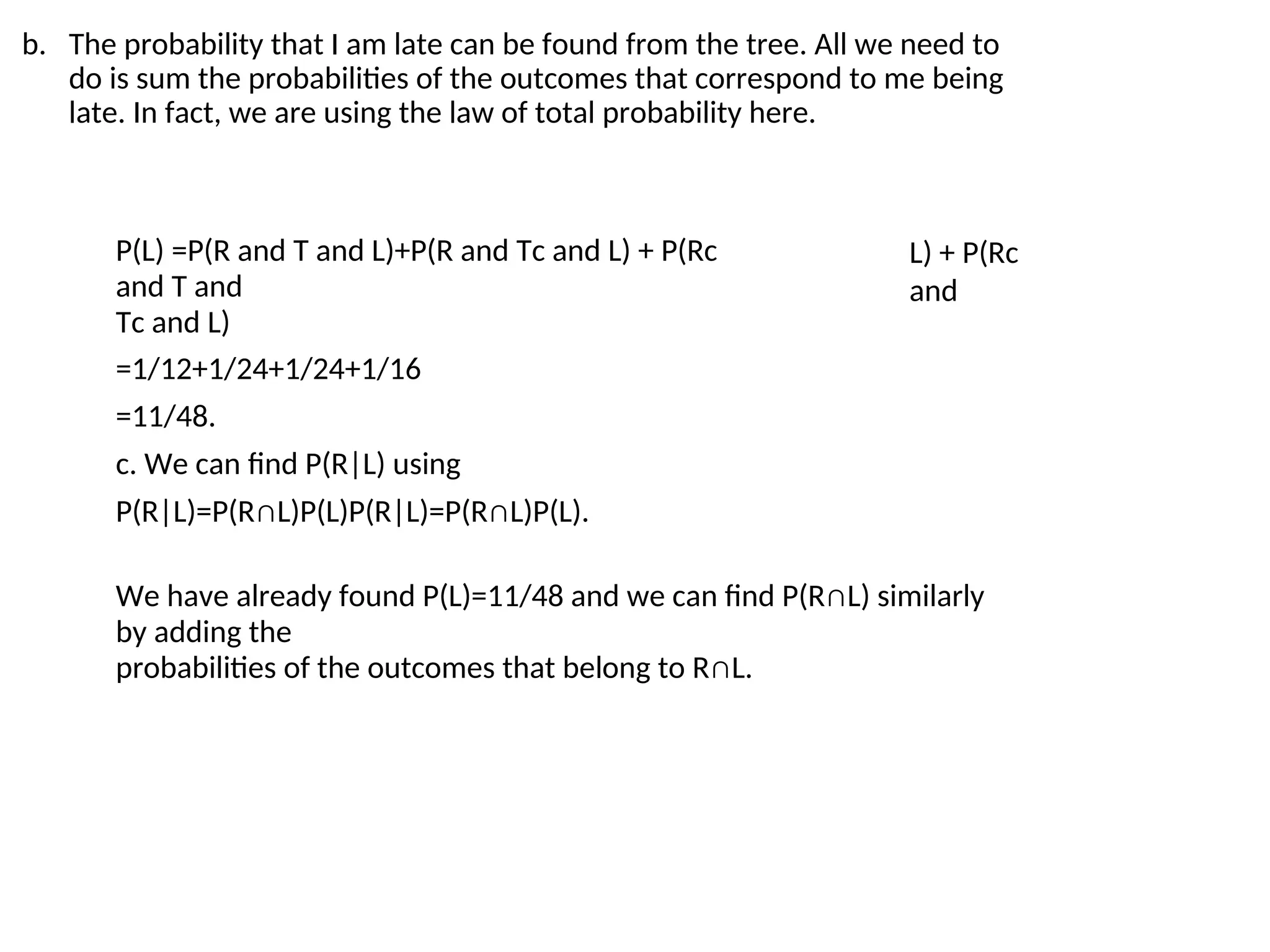
b. The probabilitythat I am late can be found from the tree. All we need to
do is sum the probabilities of the outcomes that correspond to me being
late. In fact, we are using the law of total probability here.
P(L) =P(R and T and L)+P(R and Tc and L) + P(Rc
and T and
Tc and L)
=1/12+1/24+1/24+1/16
=11/48.
c. We can find P(R|L) using
P(R|L)=P(R∩L)P(L)P(R|L)=P(R∩L)P(L).
L) + P(Rc
and
We have already found P(L)=11/48 and we can find P(R∩L) similarly
by adding the
probabilities of the outcomes that belong to R∩L.
88.
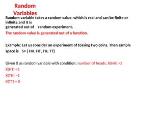
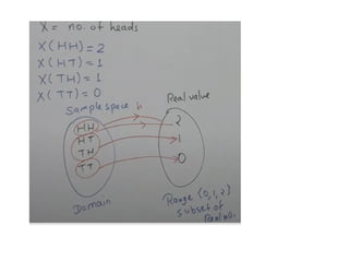
Random
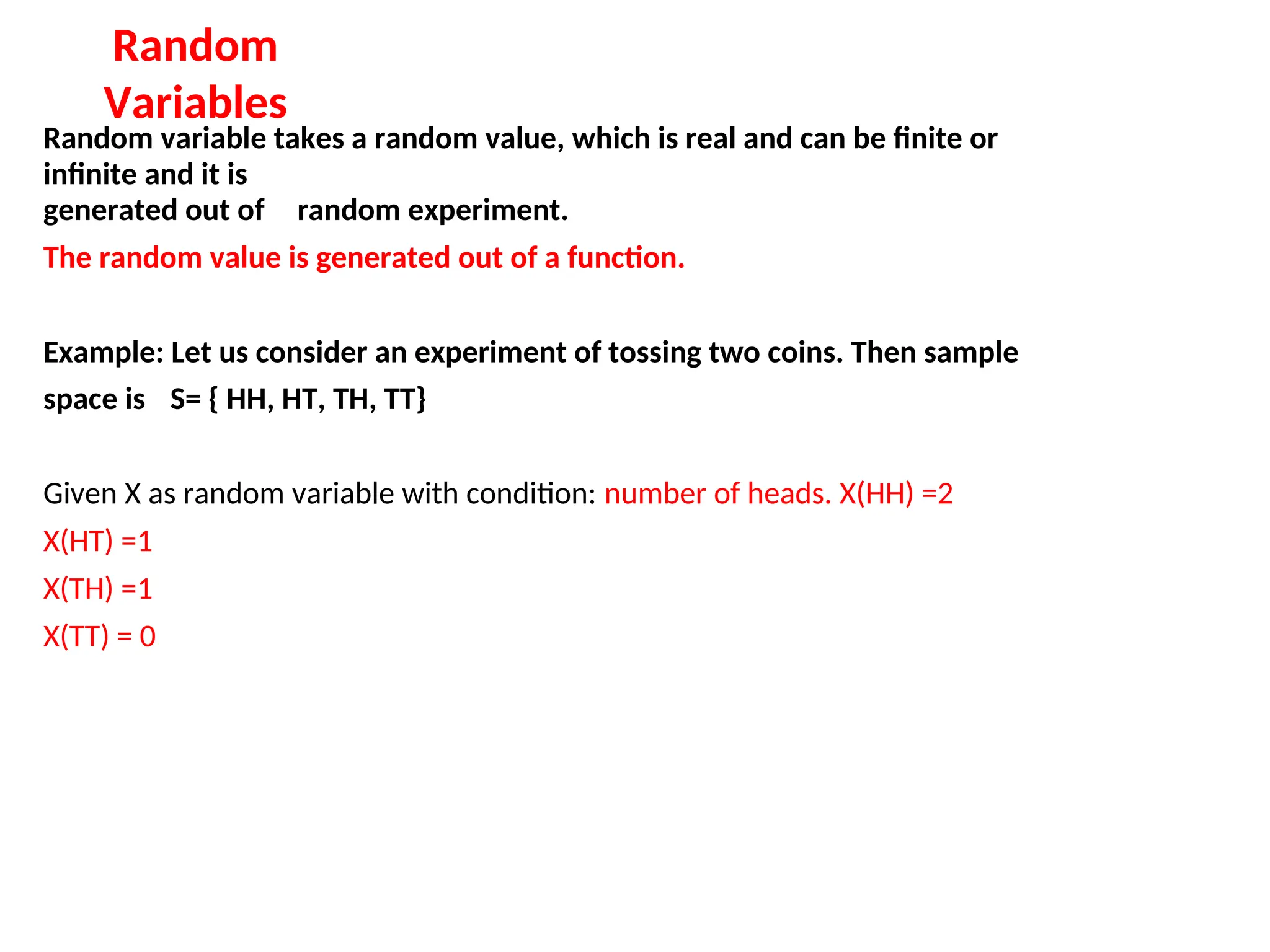
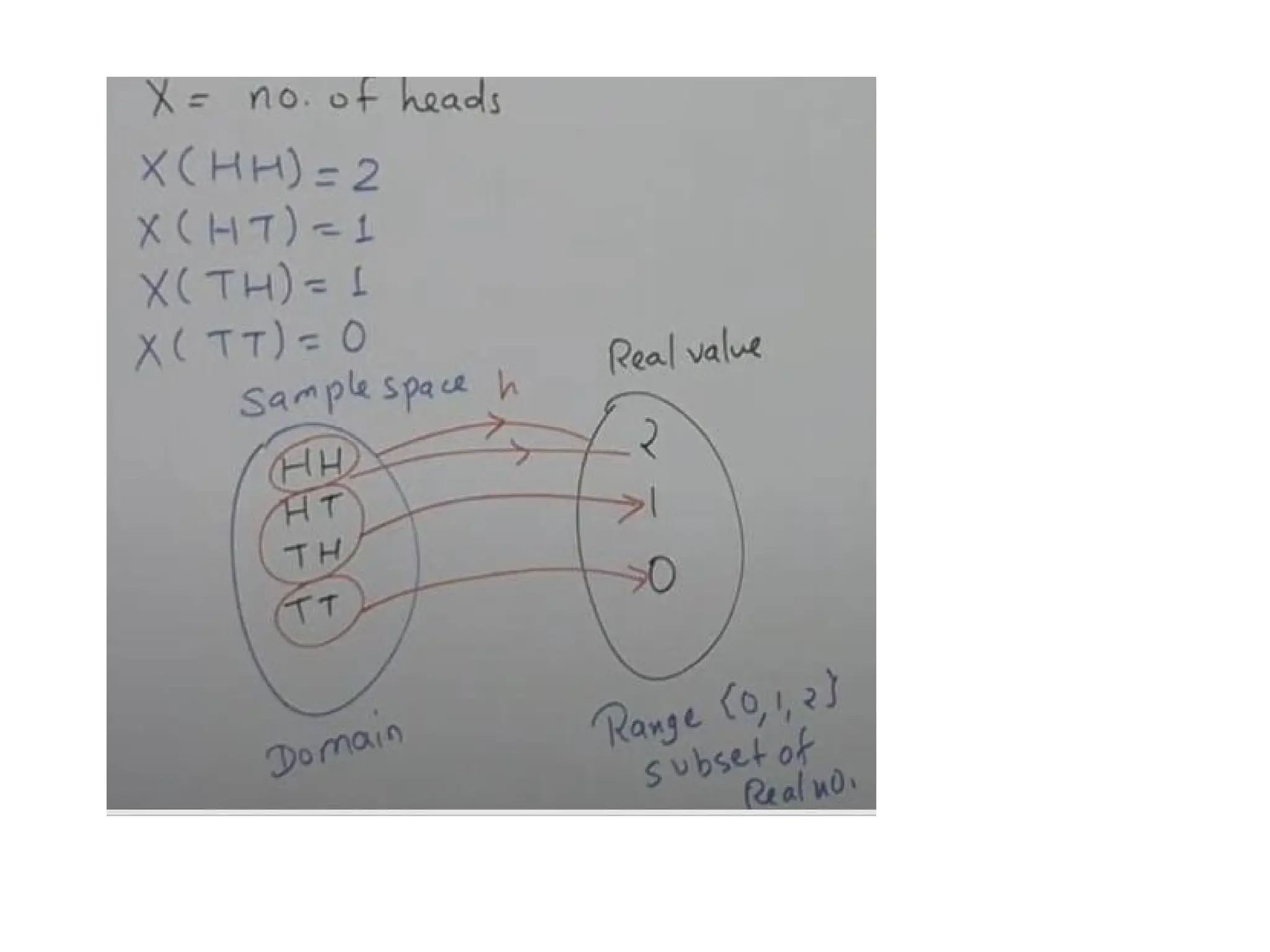
Variables
Random variable takesa random value, which is real and can be finite or
infinite and it is
generated out of random experiment.
The random value is generated out of a function.
Example: Let us consider an experiment of tossing two coins. Then sample
space is S= { HH, HT, TH, TT}
Given X as random variable with condition: number of heads. X(HH) =2
X(HT) =1
X(TH) =1
X(TT) = 0
90.
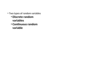
• Two typesof random variables
• Discrete random
variables
• Continuous random
variable
91.
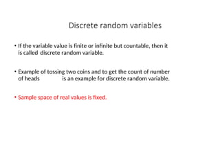
Discrete random variables
•If the variable value is finite or infinite but countable, then it
is called discrete random variable.
• Example of tossing two coins and to get the count of number
of heads is an example for discrete random variable.
• Sample space of real values is fixed.
92.
Continuous Random Variable
•If the random variable values lies between two certain fixed
numbers then it is called continuous random variable. The result
can be finite or infinite.
• Sample space of real values is not fixed, but it is in a range.
• If X is the random value and it’s values lies between a and b then,
It is represented by : a <= X <= b
Example: Temperature, age, weight, height…etc. ranges between
specific range.
Here the values for the sample space will be infinite
93.
Probability distribution
• Frequencydistribution is a listing of the observed
frequencies of all the output of an experiment that
actually occurred when experiment was done.
• Where as a probability distribution is a listing of the
probabilities of all possible outcomes that could result if
the experiment were done. (distribution with
expectations).
94.
Broad classification ofProbability distribution
• Discrete probability
distribution
• Binomial distribution
• Poisson distribution
• Continuous Probability
distribution
• Normal distribution
95.
Discrete Probability
Distribution: Binomial
Distribution
•A binomial distribution can be thought of as simply the
probability of a SUCCESS or FAILURE outcome in an
experiment or survey that is repeated multiple times.
(When we have only two possible outcomes)
• Example, a coin toss has only two possible outcomes: heads
or tails and taking a test could have two possible outcomes:
pass or fail.
96.
Assumptions of Binomial
distribution
(Itis also called as Bernoulli’s
Distribution)
• Assumptions:
• Random experiment is performed repeatedly with a fixed and finite
number of trials.
The number is denoted by ‘n’
• There are two mutually exclusive possible outcome on each trial, which
are know as “Success” and “Failure”. Success is denoted by ‘p’ and
failure is denoted by ‘q’. and p+q=1 or q=1-p.
• The outcome of any give trail does not affect the outcomes of the
subsequent trail.
That means all trials are independent.
• The probability of success and failure (p&q) remains constant for all
trials. If it does not remain constant then it is not binomial distribution.
For example tossing a coin the probability of getting head or
getting a red ball from a pool of colored balls, here every time after the
ball is taken out it is again replaced to the pool.
• With this assumption let see the formula
97.
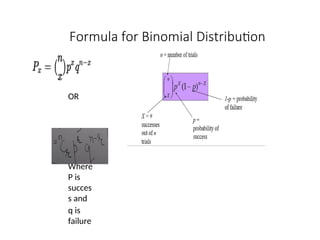
Formula for BinomialDistribution
OR
P(X=r)
=
Where
P is
succes
s and
q is
failure
98.
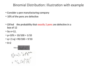
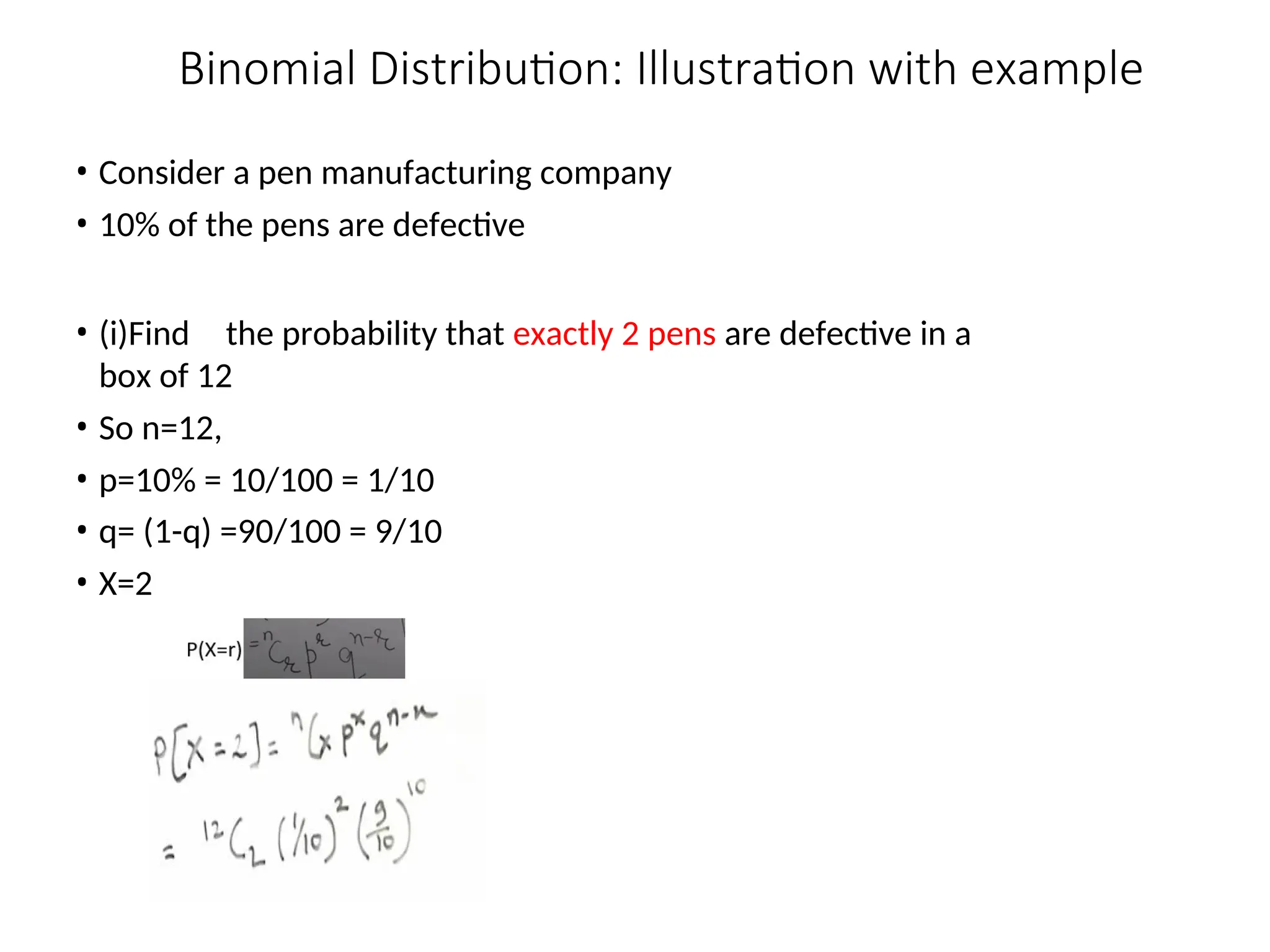
Binomial Distribution: Illustrationwith example
• Consider a pen manufacturing company
• 10% of the pens are defective
• (i)Find the probability that exactly 2 pens are defective in a
box of 12
• So n=12,
• p=10% = 10/100 = 1/10
• q= (1-q) =90/100 = 9/10
• X=2
99.
• Consider apen manufacturing company
• 10% of the pens are defective
• (i)Find the probability that at least 2 pens are defective in a
box of 12
• So n=12,
• p=10% = 10/100 = 1/10
• q= (1-q) =90/100 = 9/10
• X>=2
• P(X>=2) = 1- [P(X<2)]
• = 1-[P(X=0) +P(X=1)]
100.
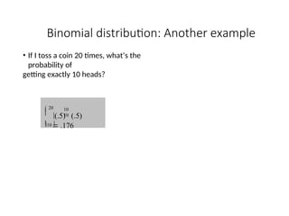
Binomial distribution: Anotherexample
• If I toss a coin 20 times, what’s the
probability of
getting exactly 10 heads?
10
10
(.5) (.5)
.176
10
20
101.
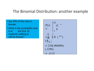
• Say 40%of the class is
female.
• What is the probability that
6 of the first 10
students walking in
will be female?
The Binomial Distribution: another example
)
1
0
6
210(.004096)
(.1296)
.1115
6
(.4 )
(.6
106
x n
x
p
q
x
n
P(x)
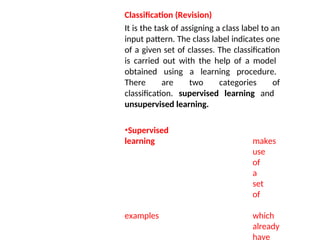
Classification (Revision)
It isthe task of assigning a class label to an
input pattern. The class label indicates one
of a given set of classes. The classification
is carried out with the help of a model
obtained using a learning procedure.
There are two categories of
classification. supervised learning and
unsupervised learning.
•Supervised
learning makes
use
of
a
set
of
examples which
already
have
105.
Learning - Continued
•Theclassifier to be designed is built
using input samples which is a mixture
of all
the classes.
•The classifier learns how to
discriminate between samples of
different
classes.
•If the Learning is offline i.e. Supervised
method then, the classifier is first
given a set of training samples and the
optimal decision boundary found, and
then
the classification is done.
•Supervised Learning refers to the
process of designing a pattern classifier
by
using a Training set of patterns to assign
class labels.
106.
Statistical / Parametricdecision
making
This refers to the situation in which we assume the general form of
probability distribution function or density function for each class.
•Statistical/Parametric Methods uses a fixed number of parameters to
build the model.
•Parametric methods are assumed to be a normal distribution.
•Parameters for using the normal distribution is –
Mean
Standard Deviation
•For each feature, we first estimate the mean and standard deviation of
the feature for each class.
107.
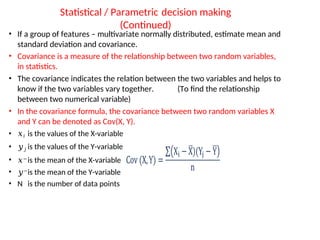
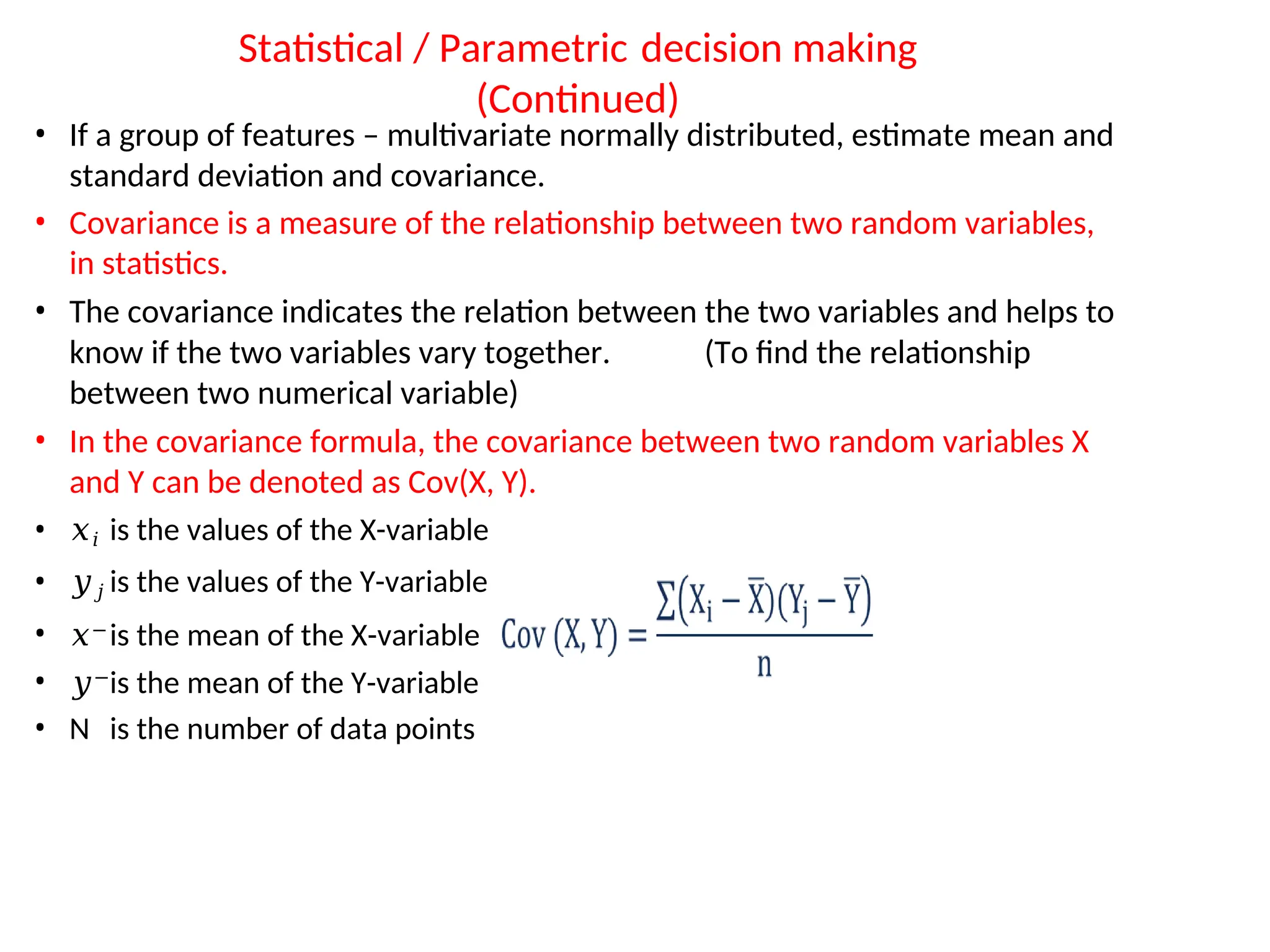
Statistical / Parametricdecision making
(Continued)
• If a group of features – multivariate normally distributed, estimate mean and
standard deviation and covariance.
• Covariance is a measure of the relationship between two random variables,
in statistics.
• The covariance indicates the relation between the two variables and helps to
know if the two variables vary together. (To find the relationship
between two numerical variable)
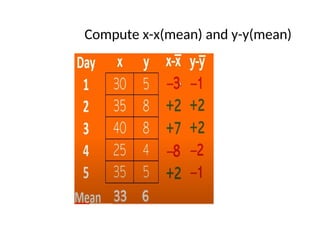
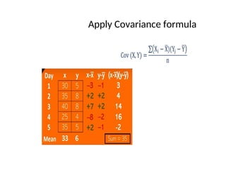
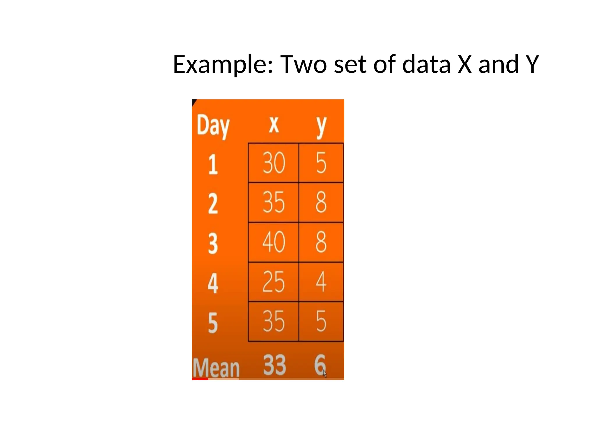
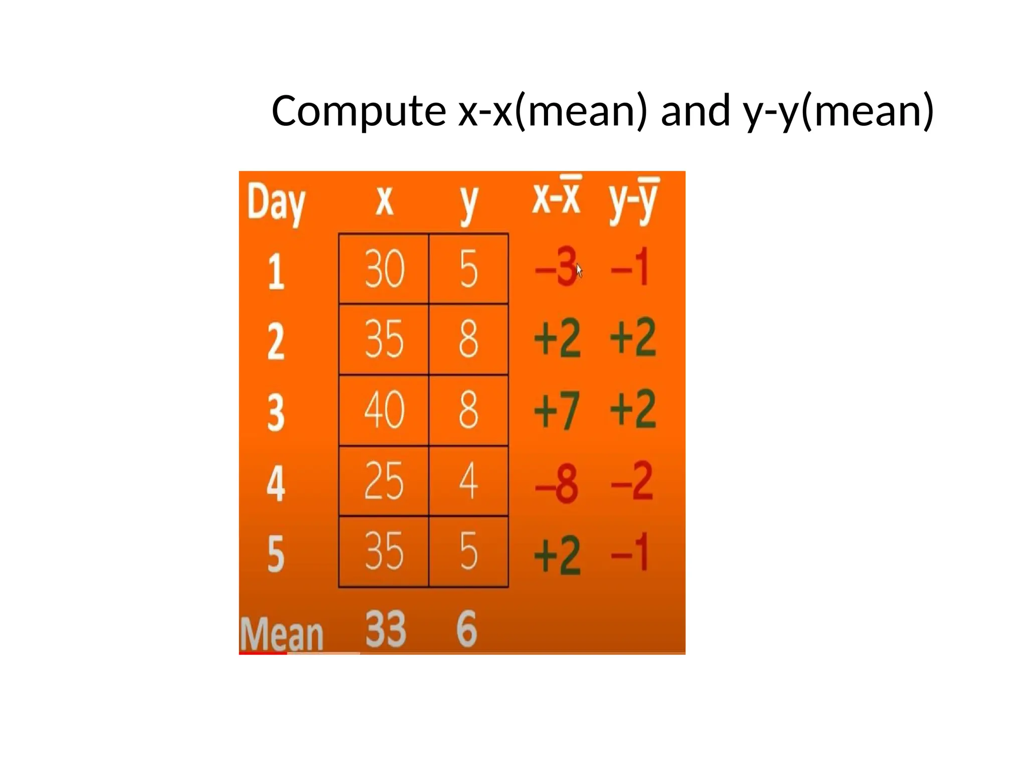
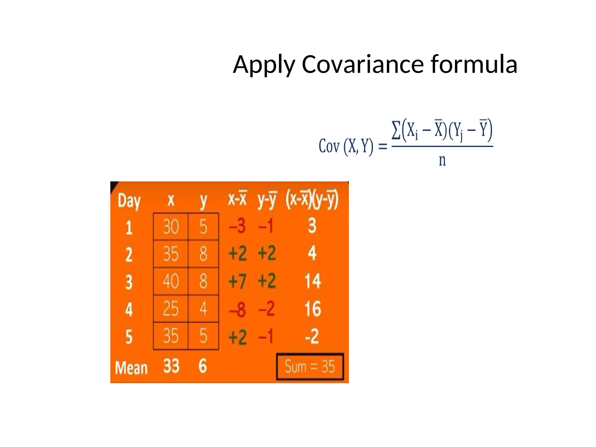
• In the covariance formula, the covariance between two random variables X
and Y can be denoted as Cov(X, Y).
• 𝑥𝑖 is the values of the X-variable
• 𝑦𝑗 is the values of the Y-variable
• 𝑥−is the mean of the X-variable
• 𝑦−
is the mean of the Y-variable
• N is the number of data points
108.
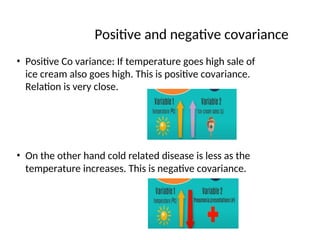
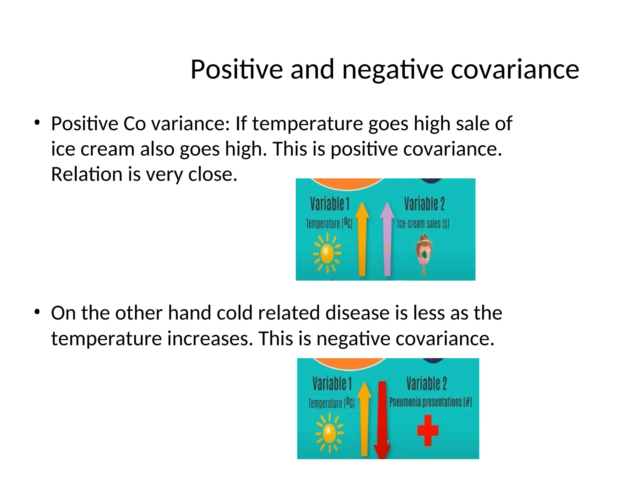
Positive and negativecovariance
• Positive Co variance: If temperature goes high sale of
ice cream also goes high. This is positive covariance.
Relation is very close.
• On the other hand cold related disease is less as the
temperature increases. This is negative covariance.
109.
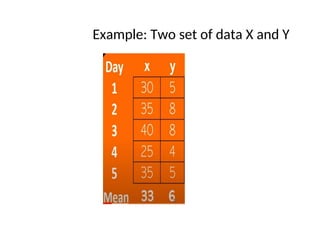
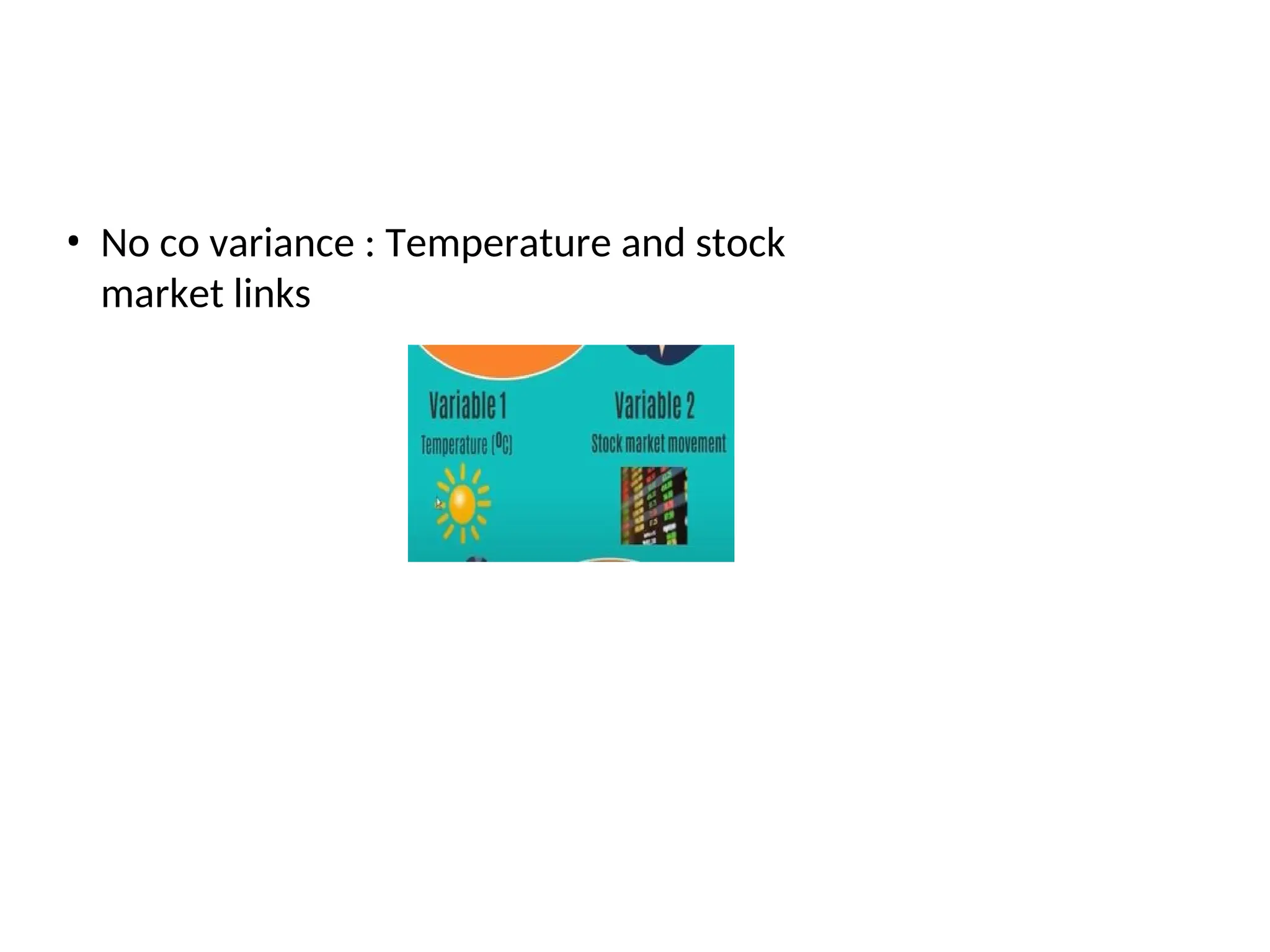
• No covariance : Temperature and stock
market links
• Final resultwill
be
35/5 = 7 = is a positive
covariance
114.
Statistical / ParametricDecision making -
continued
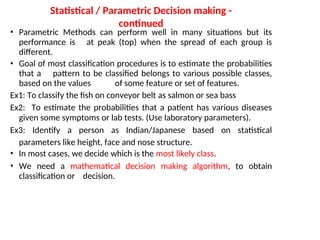
• Parametric Methods can perform well in many situations but its
performance is at peak (top) when the spread of each group is
different.
• Goal of most classification procedures is to estimate the probabilities
that a pattern to be classified belongs to various possible classes,
based on the values of some feature or set of features.
Ex1: To classify the fish on conveyor belt as salmon or sea bass
Ex2: To estimate the probabilities that a patient has various diseases
given some symptoms or lab tests. (Use laboratory parameters).
Ex3: Identify a person as Indian/Japanese based on statistical
parameters like height, face and nose structure.
• In most cases, we decide which is the most likely class.
• We need a mathematical decision making algorithm, to obtain
classification or decision.
115.
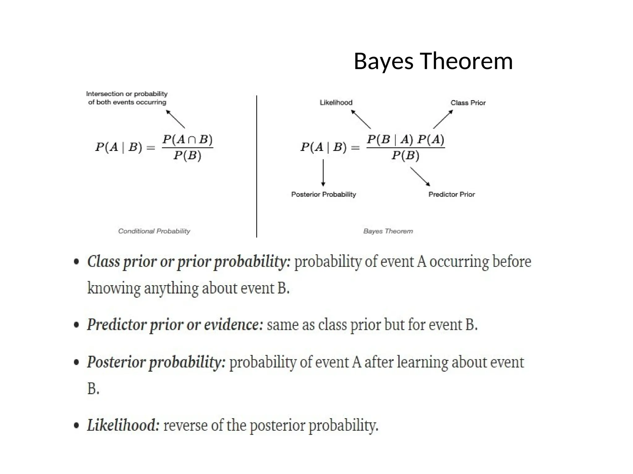
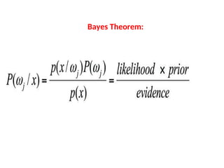
Bayes Theorem
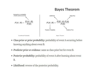
When thejoint probability, P(A∩B), is hard to
calculate or if the inverse or Bayes
probability, P(B|A), is easier to calculate then Bayes theorem can be applied.
Revisiting conditional probability
Suppose that we are interested in computing the probability of event A and
we have been told event B has occurred.
Then the conditional probability of A given B is defined to be:
P B
P A B
P A B if PB 0
Similarl
y,
P[B|A] =
if P[A] is not equal
to 0
P[A B]
P[A]
116.
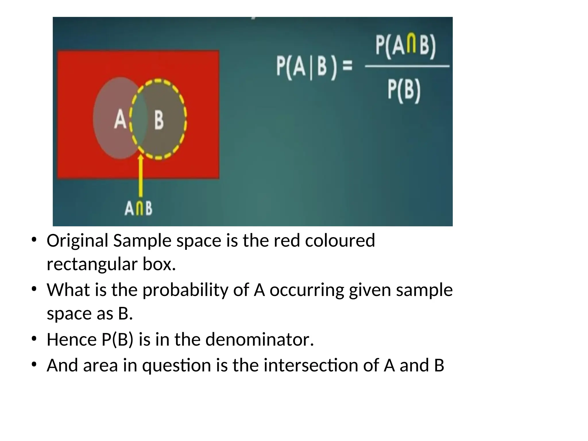
• Original Samplespace is the red coloured
rectangular box.
• What is the probability of A occurring given sample
space as B.
• Hence P(B) is in the denominator.
• And area in question is the intersection of A and B
117.
an
d
From the aboveexpressions, we can rewrite
P[A B] = P[B].P[A|B]
and P[A B] = P[A].P[B|A]
This can also be used to calculate P[A B]
So
P[A B] = P[B].P[A|B] = P[A].P[B|A]
or P[B].P[A|B] = P[A].P[B|A]
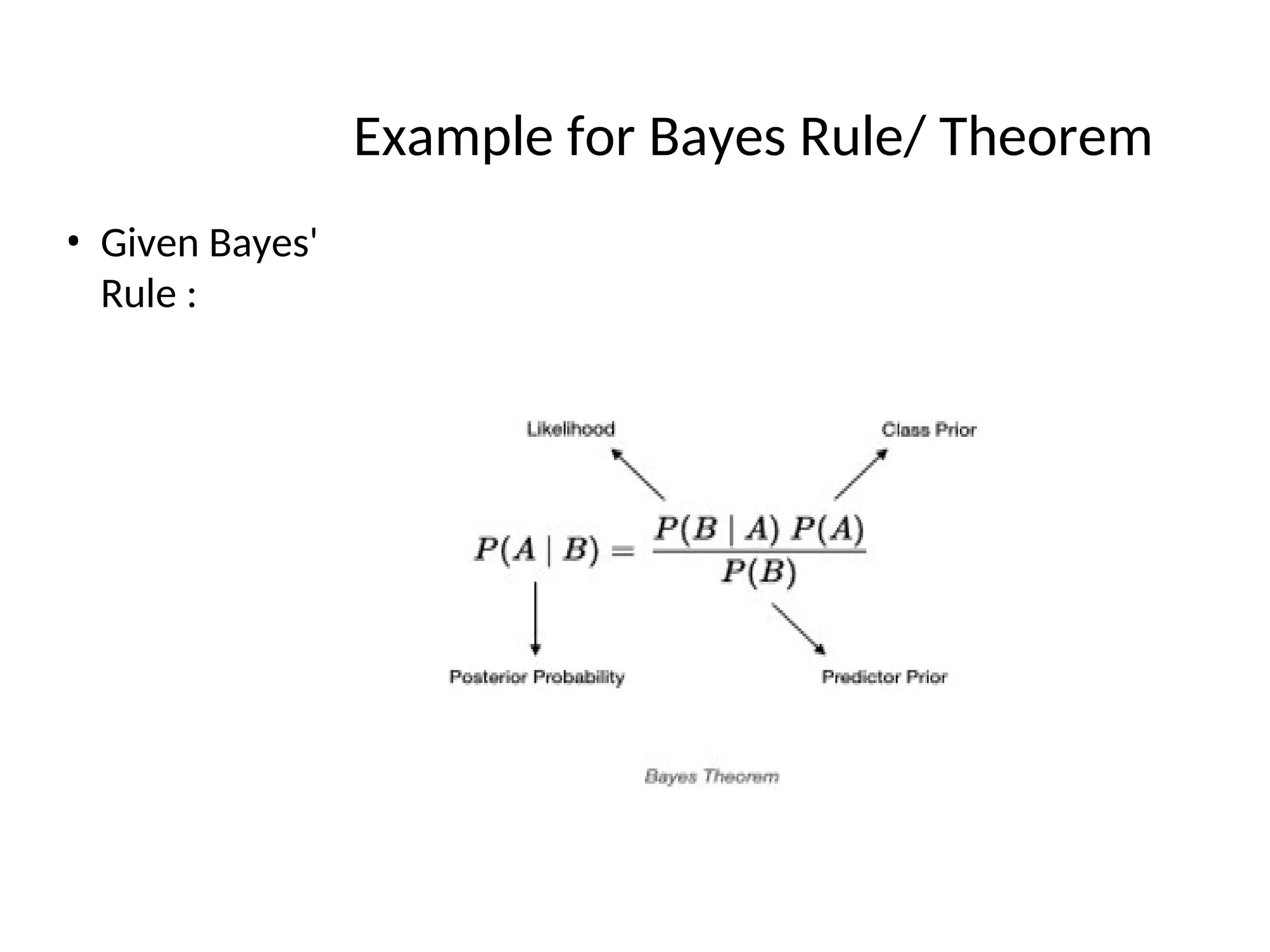
P[A|B] = P[A].P[B|A] / P[B] - Bayes Rule
PB
P A B
P A B
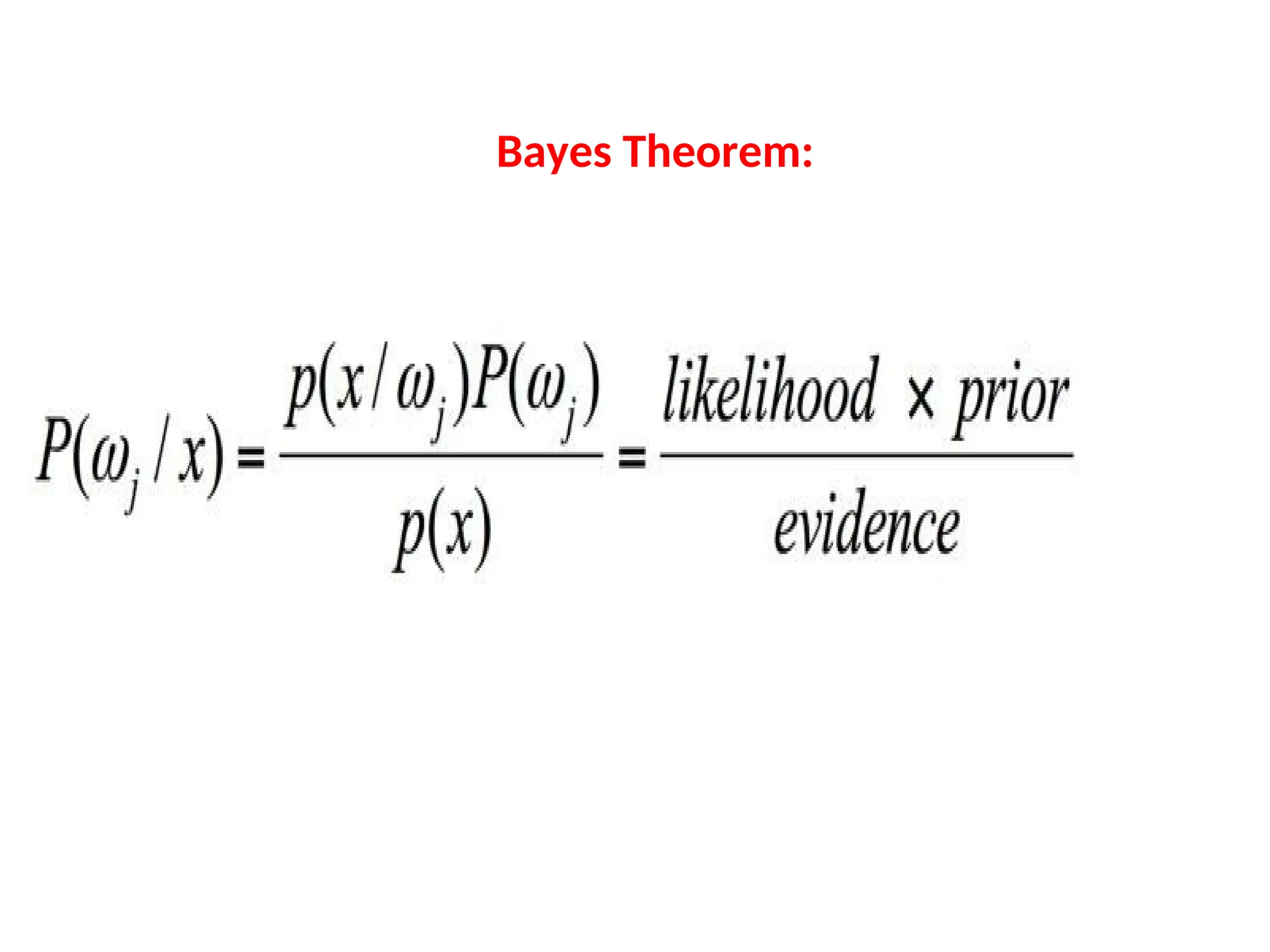
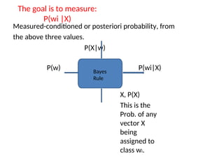
The goal isto measure:
P(wi |X)
Measured-conditioned or posteriori probability, from
the above three values.
P(X|w)
P(w) P(wi|X)
X, P(X)
This is the
Prob. of any
vector X
being
assigned to
class wi.
Bayes
Rule
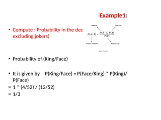
Example1:
• Compute :Probability in the deck of cards (52
excluding jokers)
• Probability of (King/Face)
• It is given by P(King/Face) = P(Face/King) * P(King)/
P(Face)
= 1 * (4/52) / (12/52)
= 1/3
123.
Example
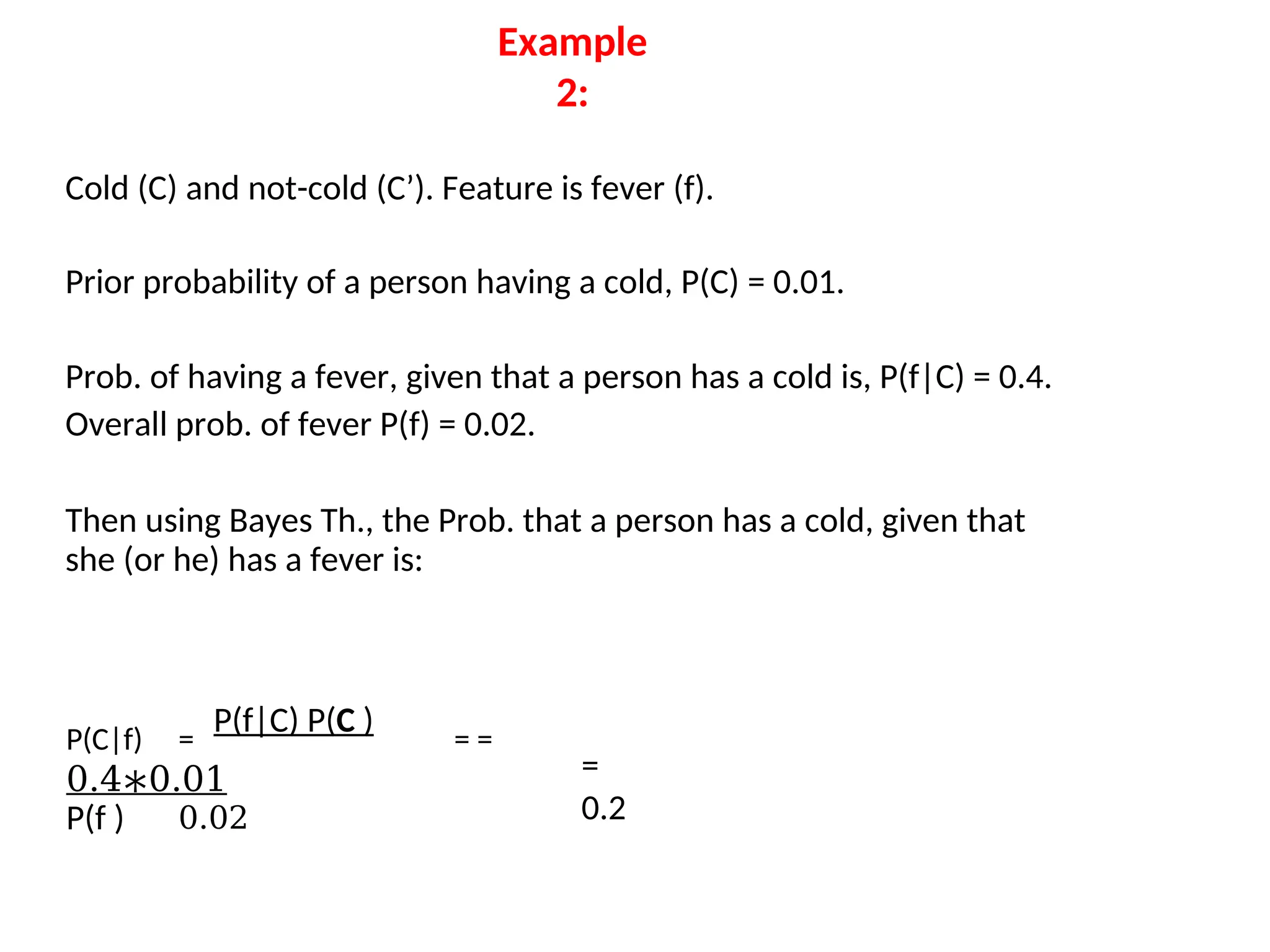
2:
Cold (C) andnot-cold (C’). Feature is fever (f).
Prior probability of a person having a cold, P(C) = 0.01.
Prob. of having a fever, given that a person has a cold is, P(f|C) = 0.4.
Overall prob. of fever P(f) = 0.02.
Then using Bayes Th., the Prob. that a person has a cold, given that
she (or he) has a fever is:
P(C|f) =
P(f|C) P(C )
= =
0.4∗0.01
P(f ) 0.02
=
0.2
124.
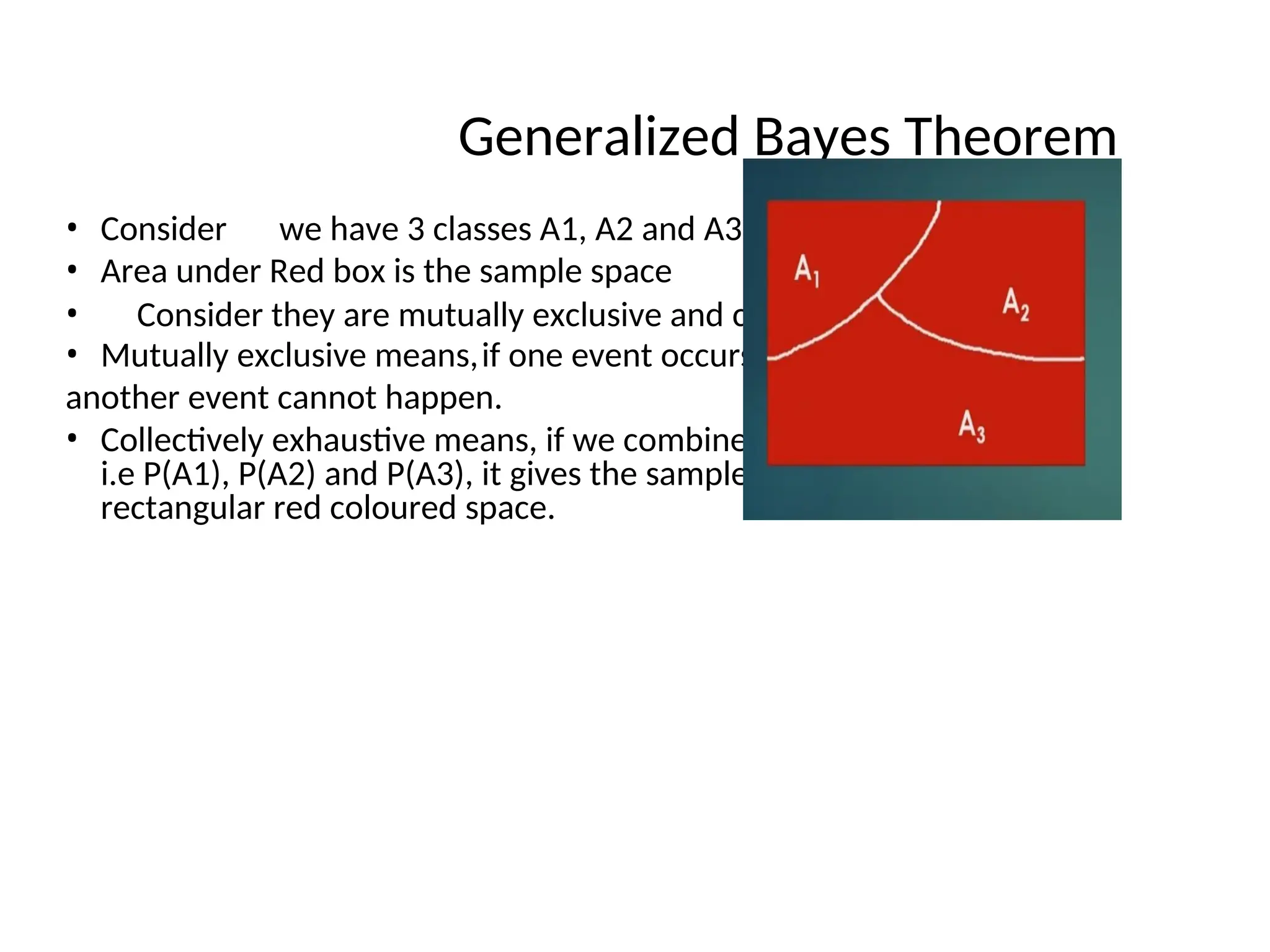
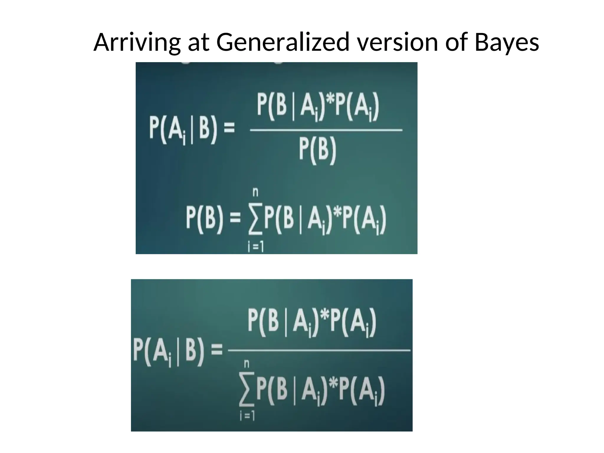
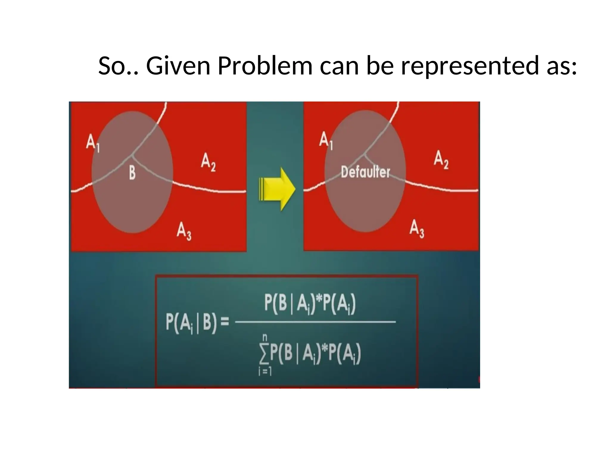
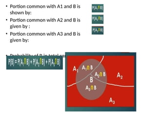
Generalized Bayes Theorem
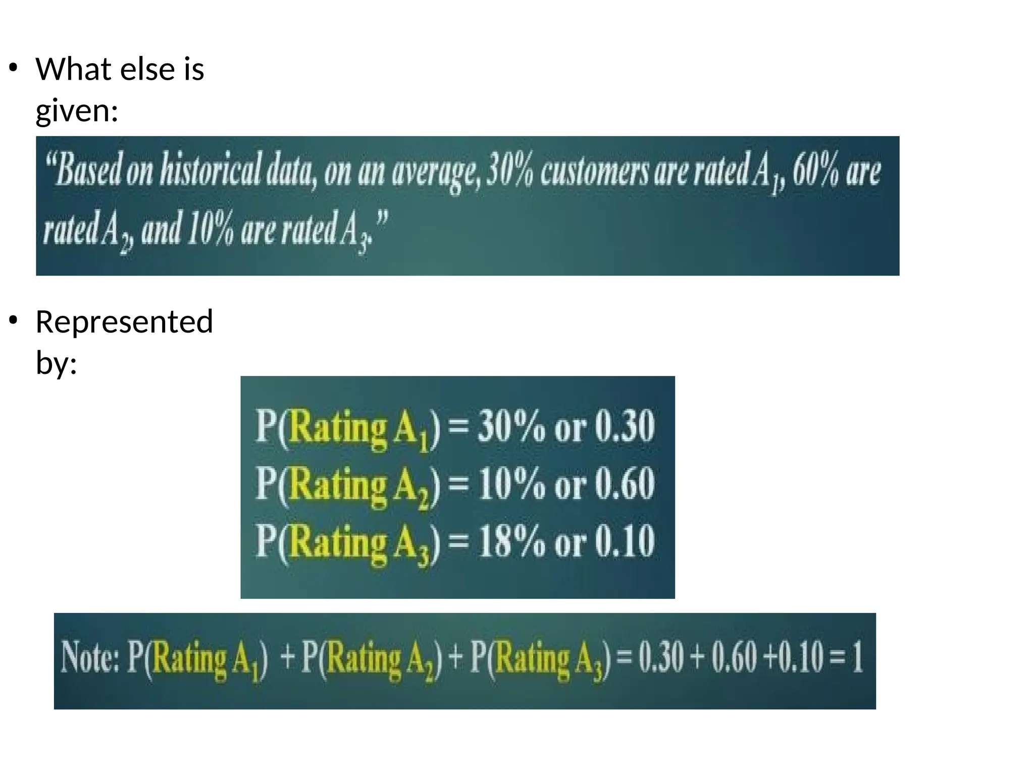
•Consider we have 3 classes A1, A2 and A3.
• Area under Red box is the sample space
• Consider they are mutually exclusive and collectively exhaustive.
• Mutually exclusive means,if one event occurs then
another event cannot happen.
• Collectively exhaustive means, if we combine all the probabilities,
i.e P(A1), P(A2) and P(A3), it gives the sample space, i.e the total
rectangular red coloured space.
125.
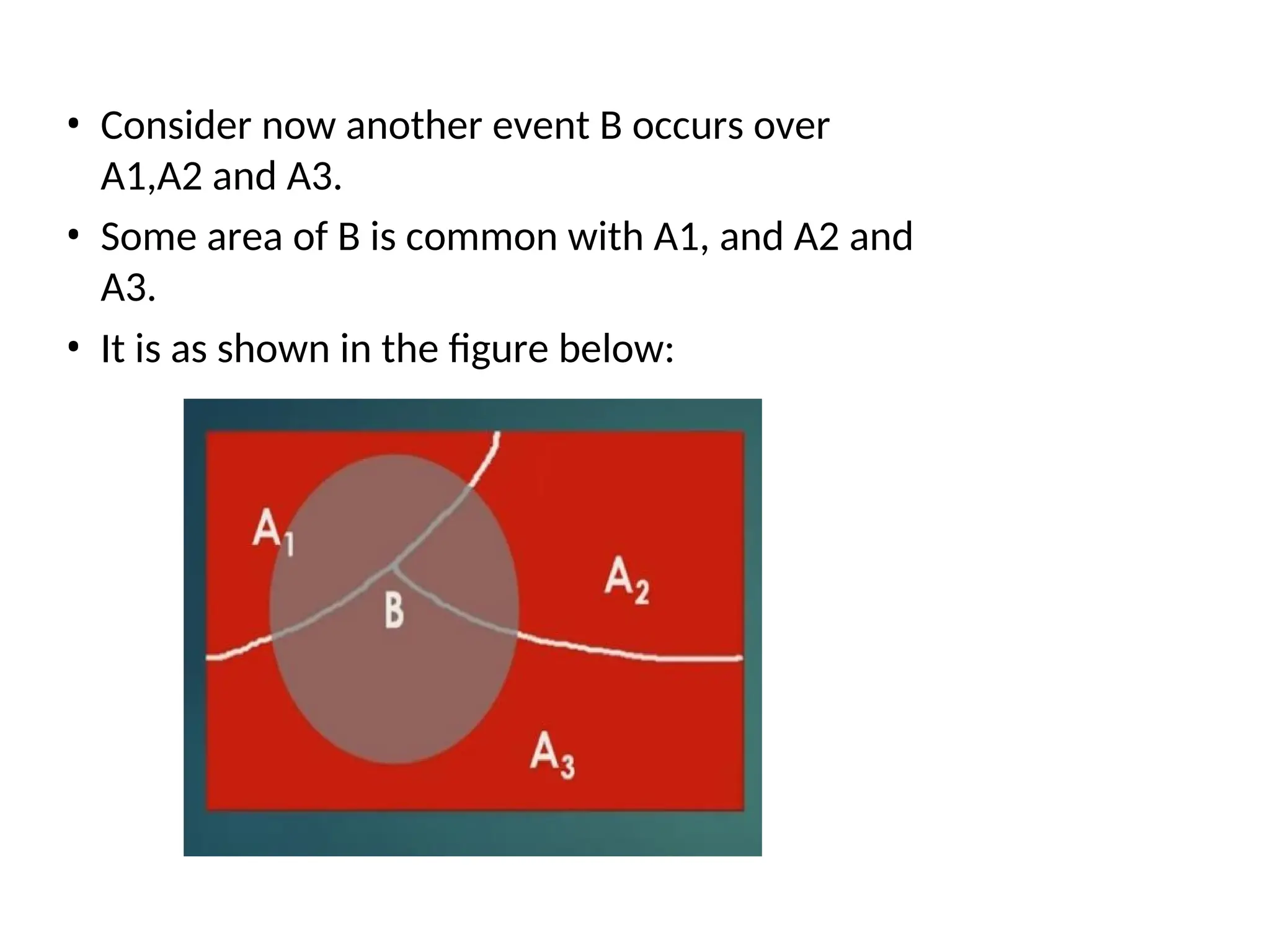
• Consider nowanother event B occurs over
A1,A2 and A3.
• Some area of B is common with A1, and A2 and
A3.
• It is as shown in the figure below:
126.
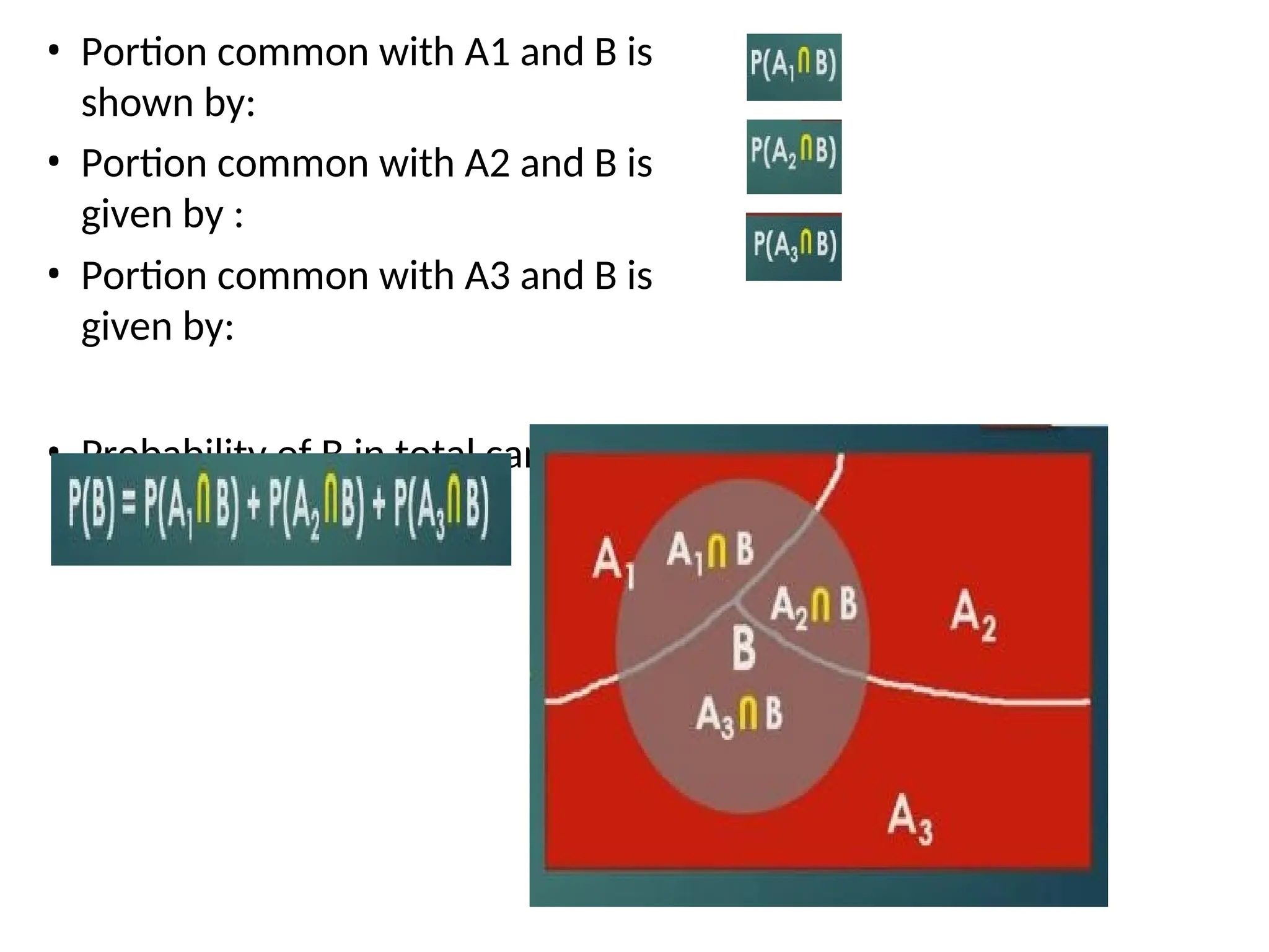
• Portion commonwith A1 and B is
shown by:
• Portion common with A2 and B is
given by :
• Portion common with A3 and B is
given by:
• Probability of B in total can be given
by
127.
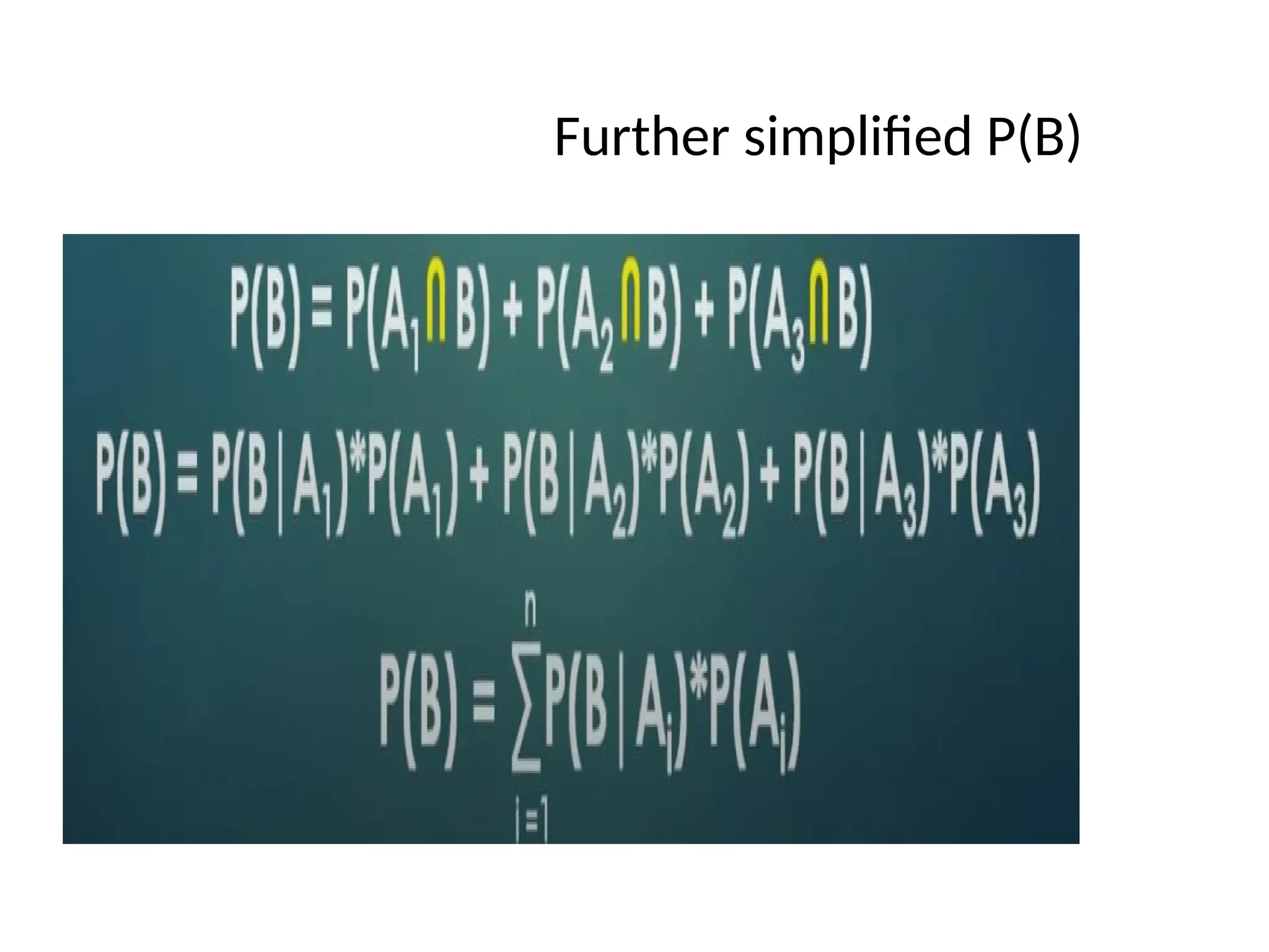
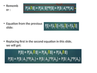
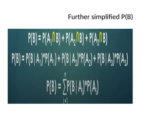
• Rememb
er :
•Equation from the previous
slide:
• Replacing first in the second equation in this slide,
we will get:
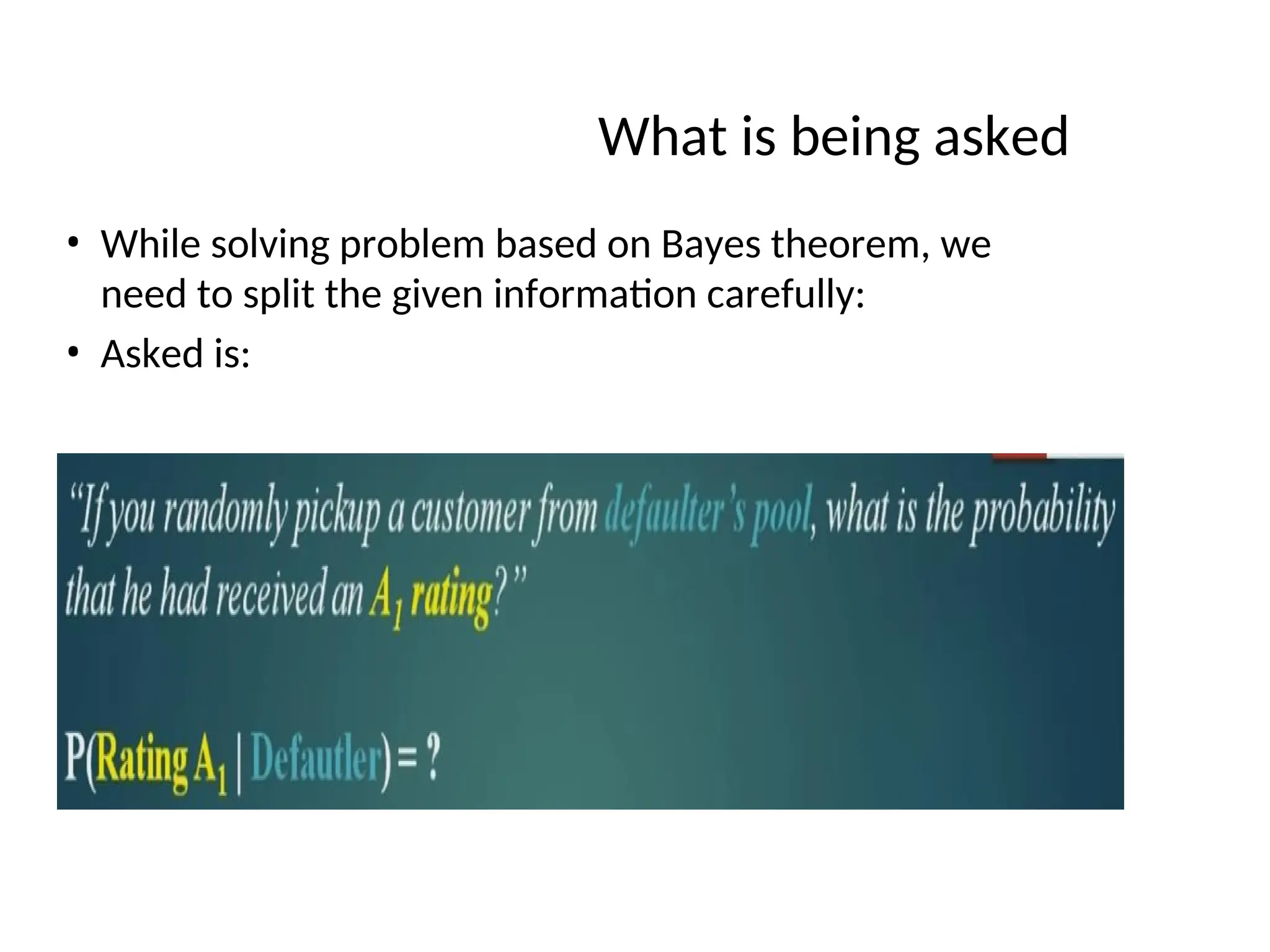
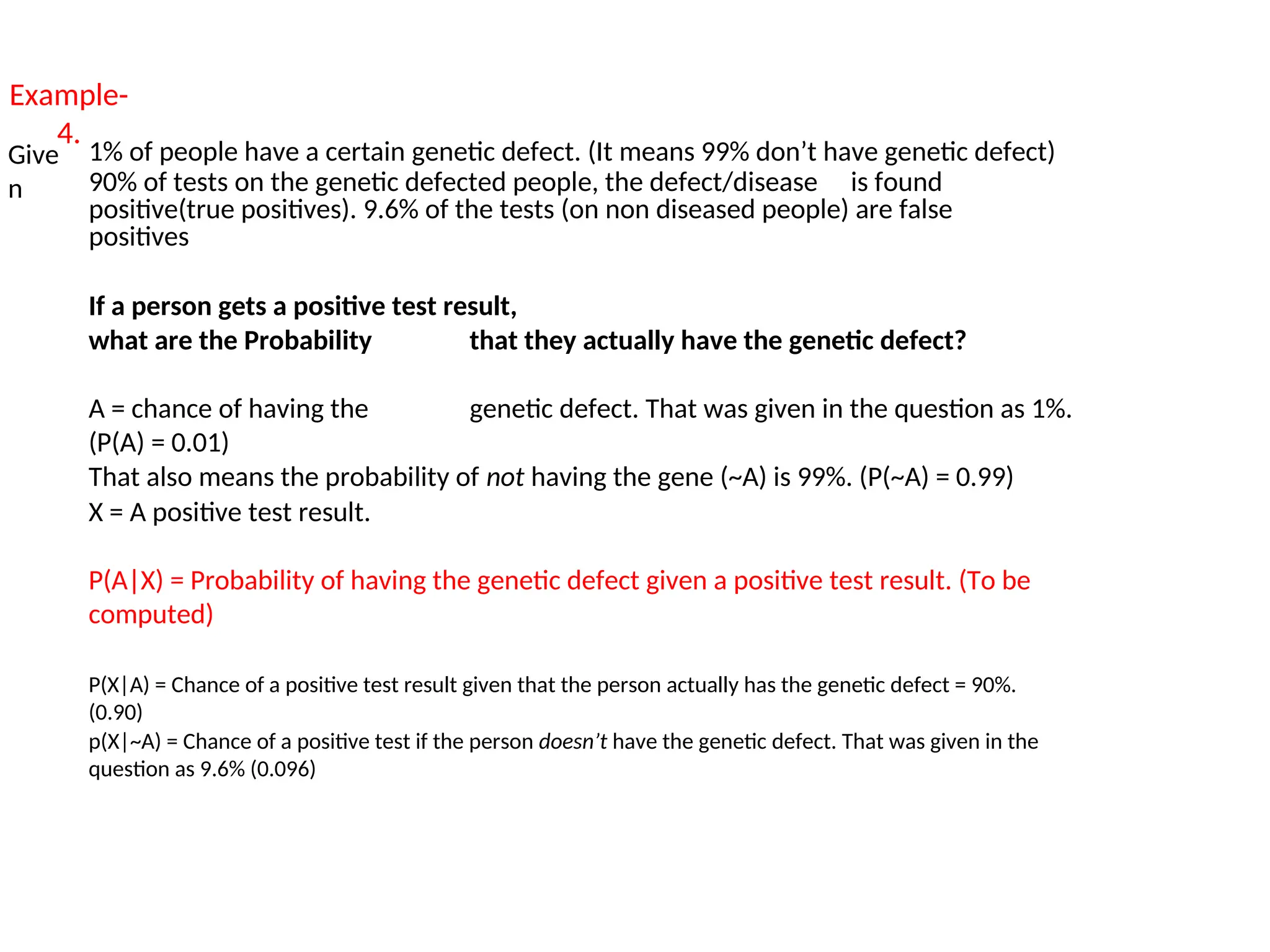
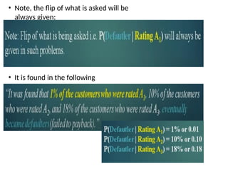
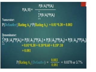
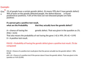
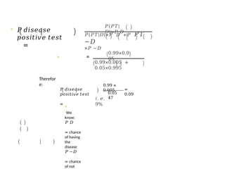
Example-
4.
Give
n
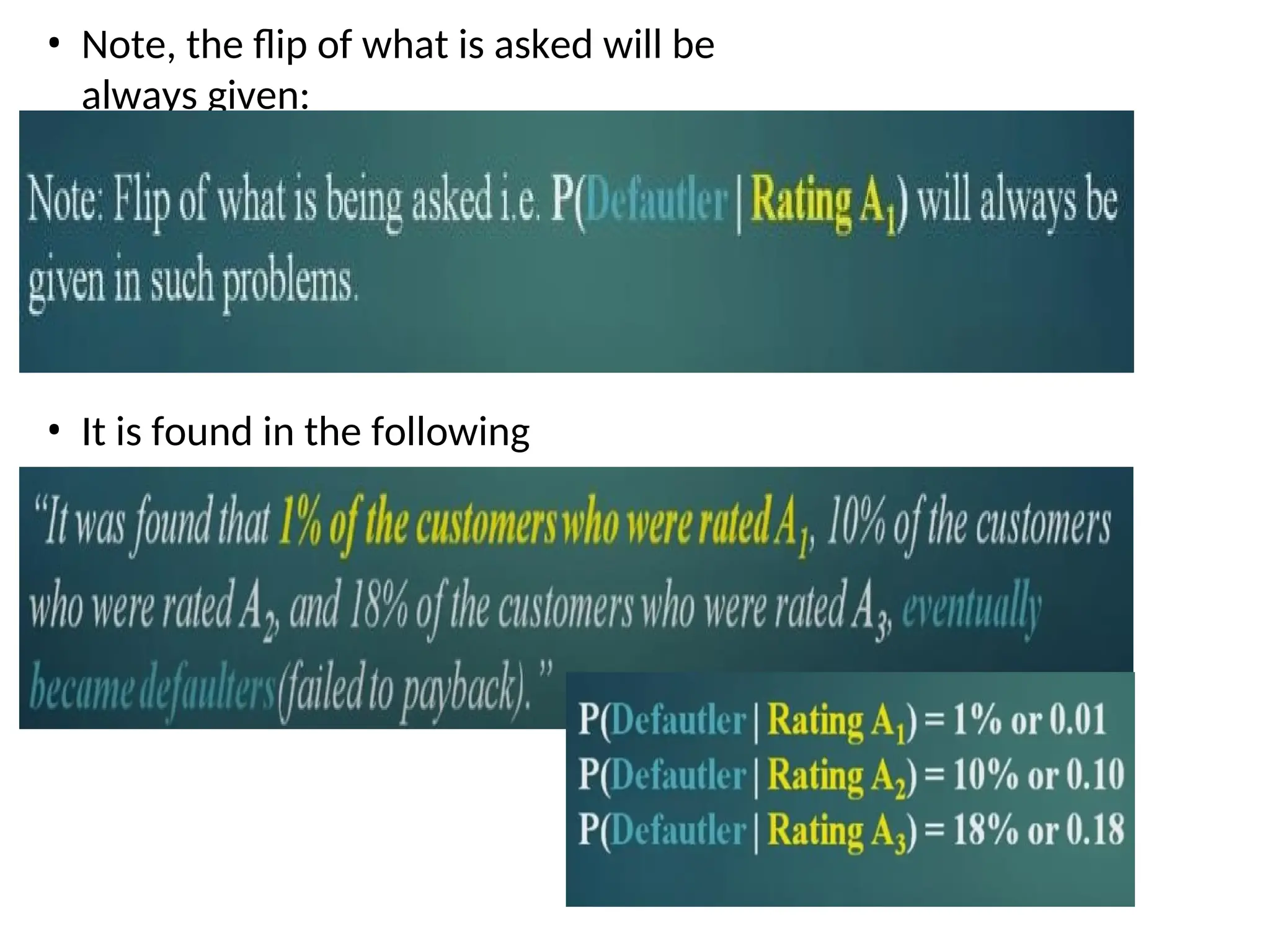
1% of peoplehave a certain genetic defect. (It means 99% don’t have genetic defect)
90% of tests on the genetic defected people, the defect/disease is found
positive(true positives). 9.6% of the tests (on non diseased people) are false
positives
If a person gets a positive test result,
what are the Probability that they actually have the genetic defect?
A = chance of having the genetic defect. That was given in the question as 1%.
(P(A) = 0.01)
That also means the probability of not having the gene (~A) is 99%. (P(~A) = 0.99)
X = A positive test result.
P(A|X) = Probability of having the genetic defect given a positive test result. (To be
computed)
P(X|A) = Chance of a positive test result given that the person actually has the genetic defect = 90%.
(0.90)
p(X|~A) = Chance of a positive test if the person doesn’t have the genetic defect. That was given in the
question as 9.6% (0.096)
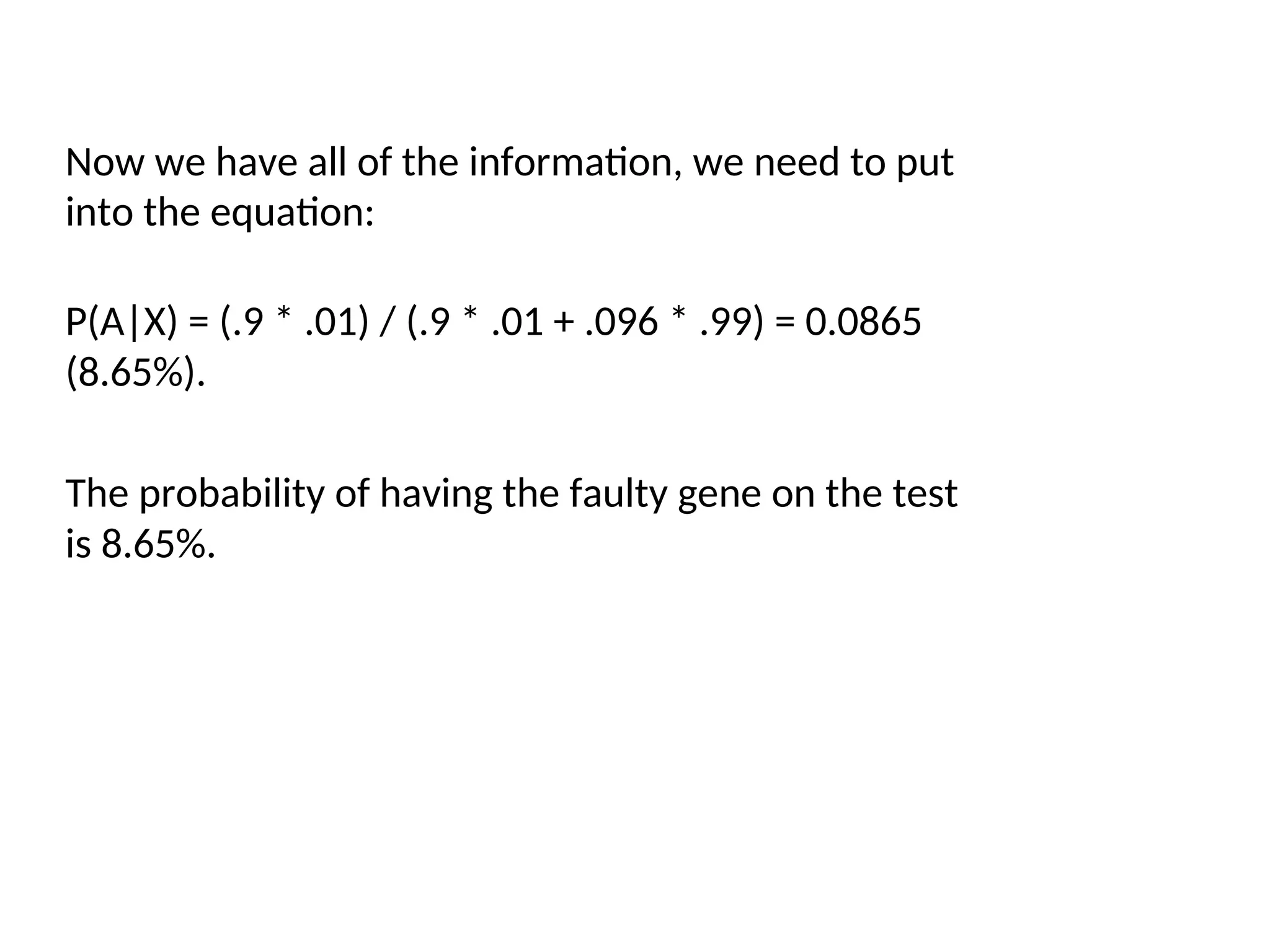
137.
Now we haveall of the information, we need to put
into the equation:
P(A|X) = (.9 * .01) / (.9 * .01 + .096 * .99) = 0.0865
(8.65%).
The probability of having the faulty gene on the test
is 8.65%.
138.
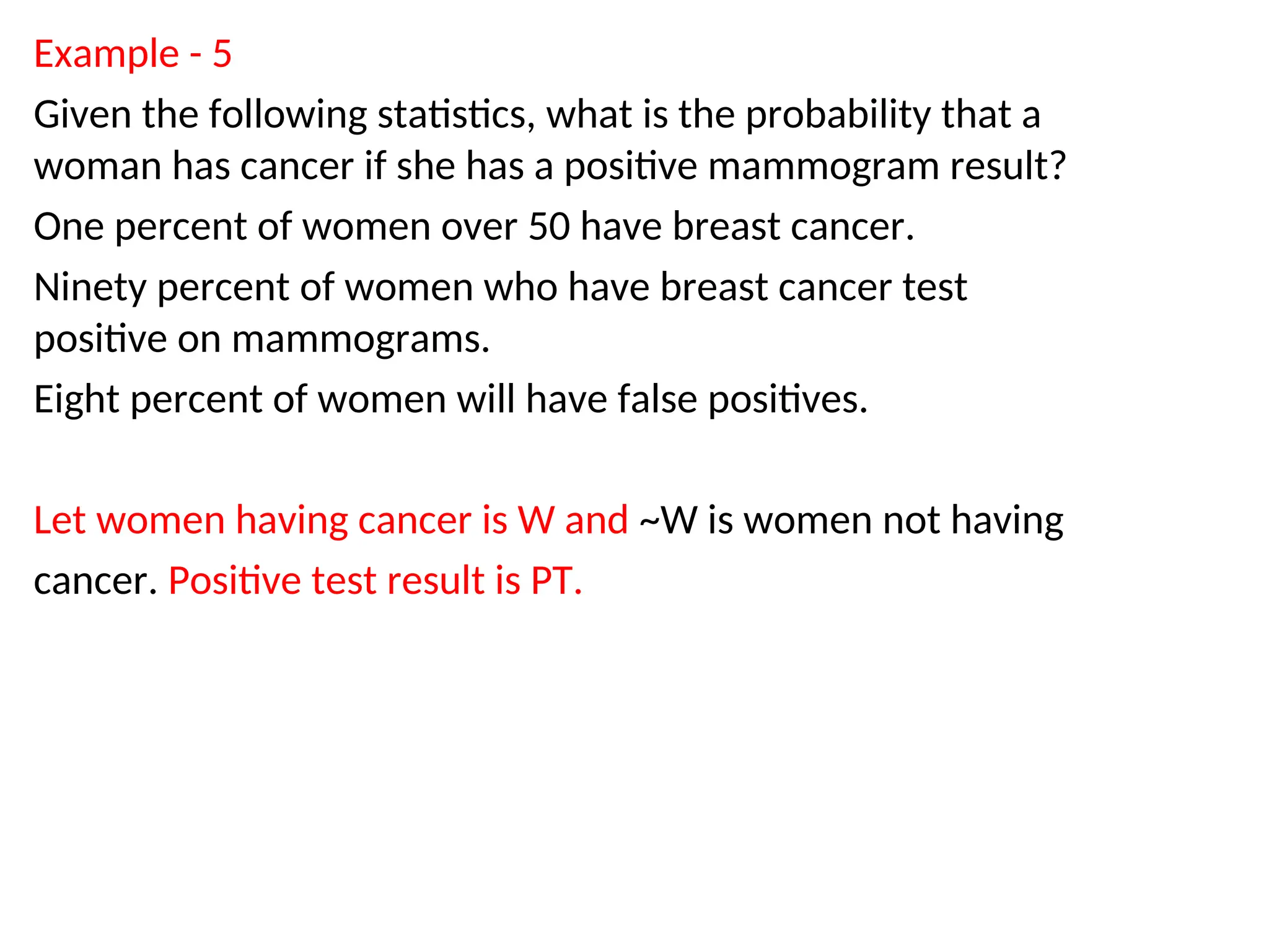
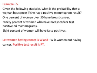
Example - 5
Giventhe following statistics, what is the probability that a
woman has cancer if she has a positive mammogram result?
One percent of women over 50 have breast cancer.
Ninety percent of women who have breast cancer test
positive on mammograms.
Eight percent of women will have false positives.
Let women having cancer is W and ~W is women not having
cancer. Positive test result is PT.
139.
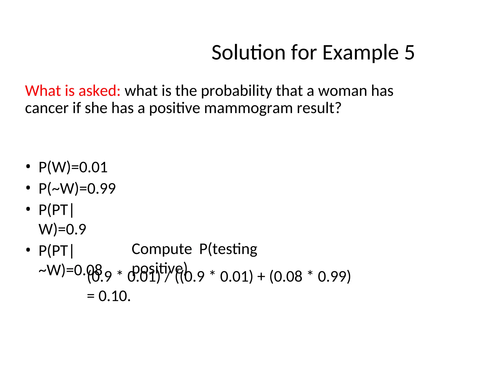
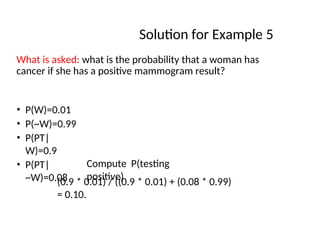
Solution for Example5
What is asked: what is the probability that a woman has
cancer if she has a positive mammogram result?
• P(W)=0.01
• P(~W)=0.99
• P(PT|
W)=0.9
• P(PT|
~W)=0.08
Compute P(testing
positive)
(0.9 * 0.01) / ((0.9 * 0.01) + (0.08 * 0.99)
= 0.10.
140.
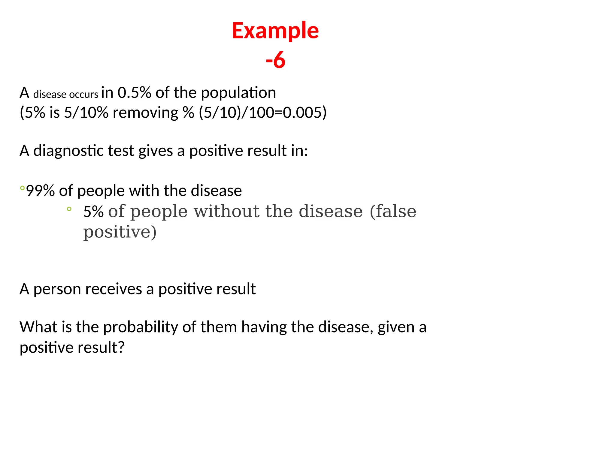
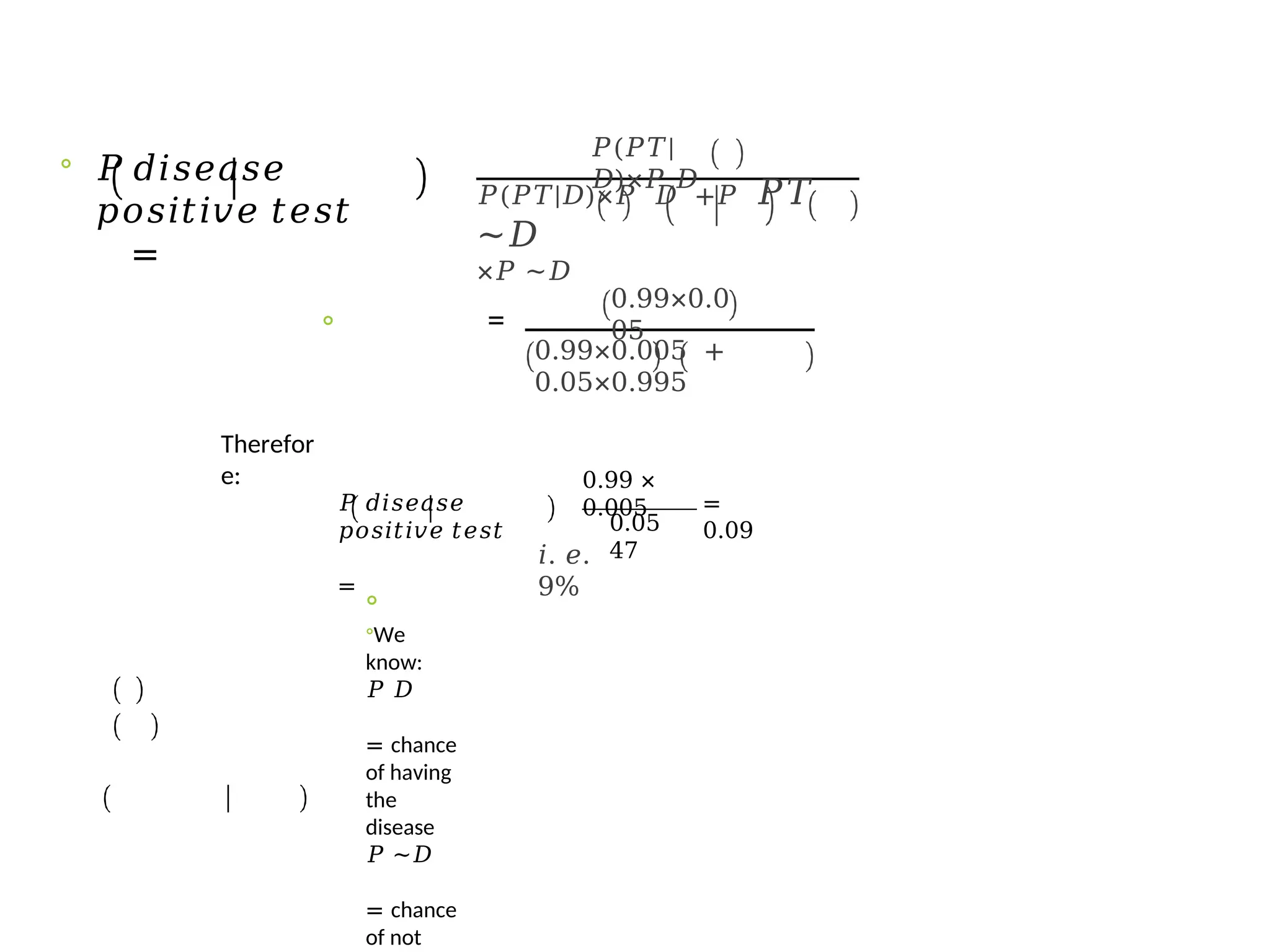
Example
-6
A disease occursin 0.5% of the population
(5% is 5/10% removing % (5/10)/100=0.005)
A diagnostic test gives a positive result in:
◦99% of people with the disease
◦ 5% of people without the disease (false
positive)
A person receives a positive result
What is the probability of them having the disease, given a
positive result?
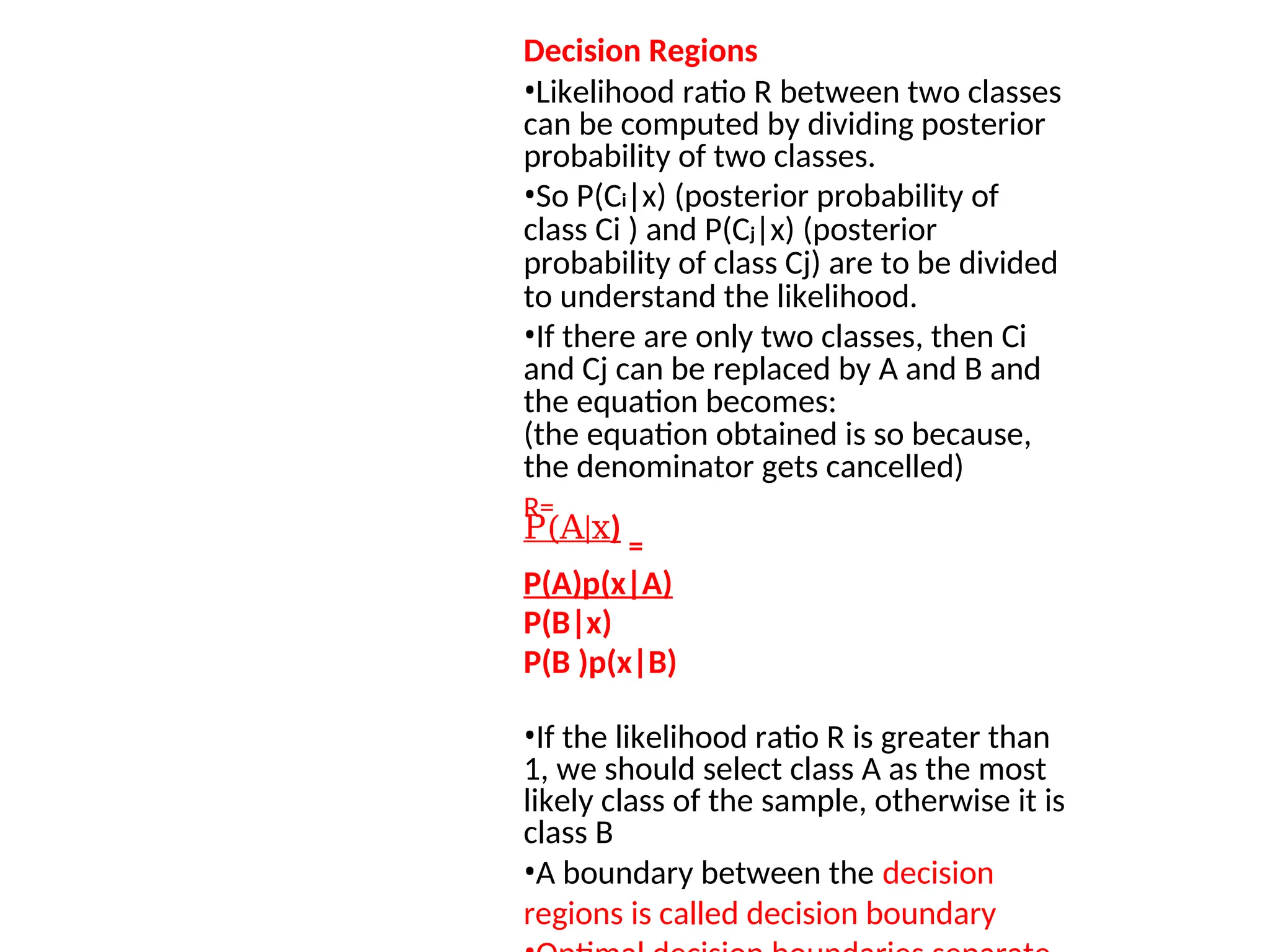
Decision Regions
•Likelihood ratioR between two classes
can be computed by dividing posterior
probability of two classes.
•So P(Ci|x) (posterior probability of
class Ci ) and P(Cj|x) (posterior
probability of class Cj) are to be divided
to understand the likelihood.
•If there are only two classes, then Ci
and Cj can be replaced by A and B and
the equation becomes:
(the equation obtained is so because,
the denominator gets cancelled)
R=
P(A|x)
=
P(A)p(x|A)
P(B|x)
P(B )p(x|B)
•If the likelihood ratio R is greater than
1, we should select class A as the most
likely class of the sample, otherwise it is
class B
•A boundary between the decision
regions is called decision boundary
143.
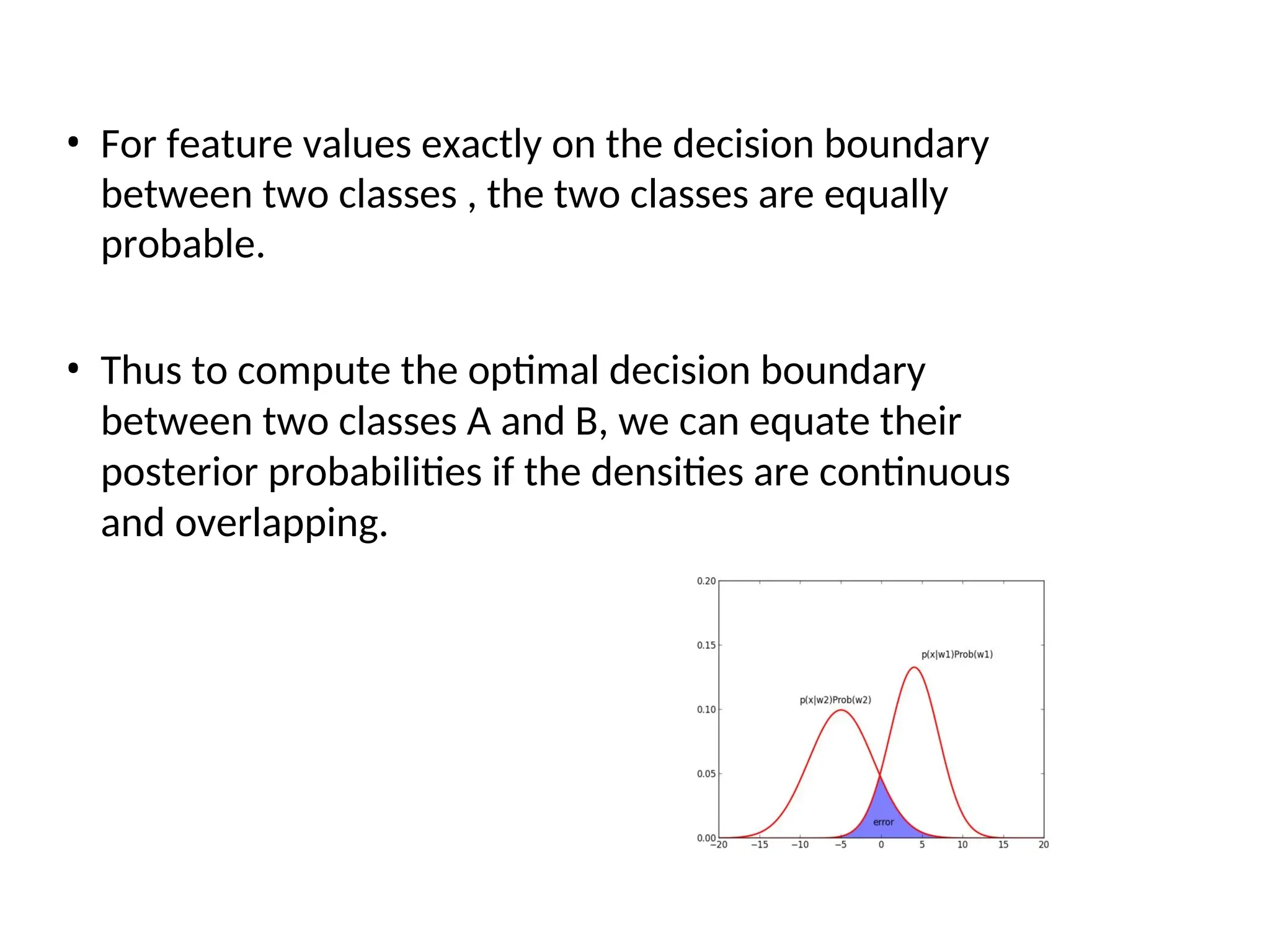
• For featurevalues exactly on the decision boundary
between two classes , the two classes are equally
probable.
• Thus to compute the optimal decision boundary
between two classes A and B, we can equate their
posterior probabilities if the densities are continuous
and overlapping.
144.
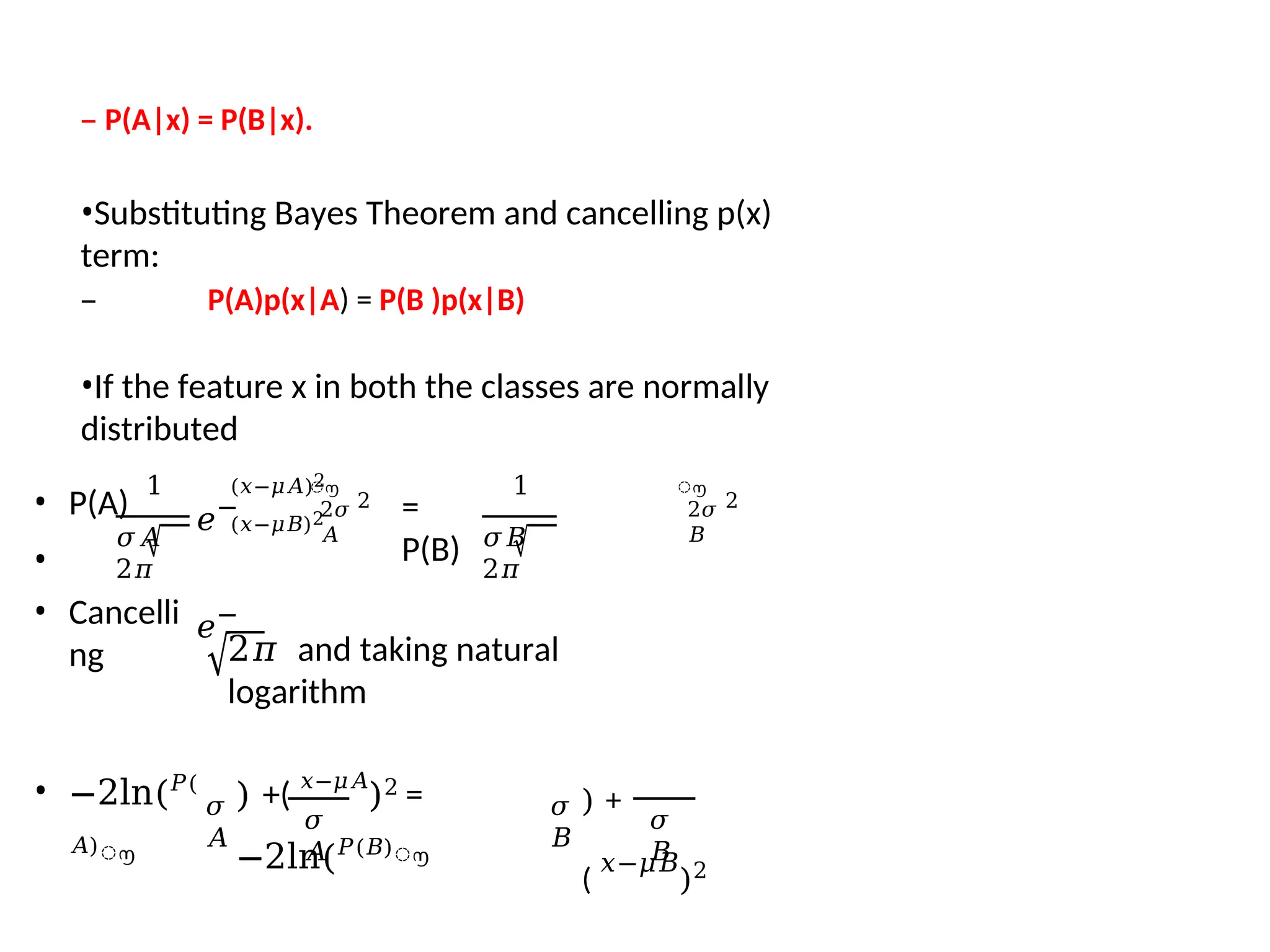
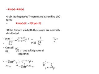
– P(A|x) =P(B|x).
•Substituting Bayes Theorem and cancelling p(x)
term:
– P(A)p(x|A) = P(B )p(x|B)
•If the feature x in both the classes are normally
distributed
1
𝜎𝐴
2𝜋
ൗ
2𝜎
𝐴
2
=
P(B)
1
𝜎𝐵
2𝜋
𝑒−
𝑒−
ൗ
(𝑥−𝜇𝐴)2
(𝑥−𝜇𝐵)2 2𝜎
𝐵
2
• P(A)
•
• Cancelli
ng 2𝜋 and taking natural
logarithm
• −2ln(𝑃(
𝐴)
ൗ
𝜎
𝐴
𝜎
𝐴
) +(
𝑥−𝜇𝐴
)2 =
−2ln(𝑃(𝐵)
ൗ
𝜎
𝐵
) +
(
𝑥−𝜇𝐵
)2
𝜎
𝐵
145.
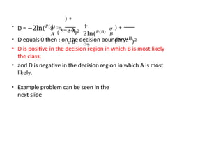
𝜎
𝐴
) +
(
𝑥−𝜇𝐴
)2
+
2ln(𝑃(𝐵)
ൗ
𝜎
𝐵
𝜎𝐴
𝜎𝐵
) +
(
𝑥−𝜇𝐵
)2
•D = −2ln(𝑃(𝐴)ൗ
• D equals 0 then : on the decision boundary;
• D is positive in the decision region in which B is most likely
the class;
• and D is negative in the decision region in which A is most
likely.
• Example problem can be seen in the
next slide


![Additive
rule
(In general)
P[A B] = P[A] + P[B] – P[A B]
or
P[A or B] = P[A] + P[B] – P[A and
B]](https://image.slidesharecdn.com/introductiontopatternrecognition-250630005914-5e4ea789/85/Introduction-to-Pattern-Recognition-NOTES-ppt-65-320.jpg)
![The additive rule (Mutually exclusive events) if A
B =
P[A B] = P[A] +
P[B]
i.e.
P[A or B] = P[A] +
P[B]
if A B =
(A and B mutually
exclusive)](https://image.slidesharecdn.com/introductiontopatternrecognition-250630005914-5e4ea789/85/Introduction-to-Pattern-Recognition-NOTES-ppt-66-320.jpg)
![Logi
c
A
B
B
A
A
B
When P[A] is added to P[B] the outcome in A B are
counted twice
hence
P[A B] = P[A] + P[B] – P[A B]](https://image.slidesharecdn.com/introductiontopatternrecognition-250630005914-5e4ea789/85/Introduction-to-Pattern-Recognition-NOTES-ppt-67-320.jpg)
![Solution:
Let A = the event that Bangalore is amongst the
final 5. Let B = the event that Mohali is amongst
the final 5.
Given P[A] = 0.20, P[B] = 0.35, and P[A B]
= 0.08
What is P[A B]?
Note: “and” ≡ , “or” ≡ .
P A B PA PB PA B
0.20 0.35 0.08 0.47](https://image.slidesharecdn.com/introductiontopatternrecognition-250630005914-5e4ea789/85/Introduction-to-Pattern-Recognition-NOTES-ppt-69-320.jpg)
![Find the probability of drawing an ace or a spade from a deck
of cards.
There are 52 cards in a deck; 13 are spades, 4 are aces.
Probability of a single card being spade is:
13/52 Probability of drawing an Ace is :
4/52
= 1/4.
=
1/13.
Probability of a single card being both Spade and Ace
= 1/52.
Let A = Event of drawing a spade . Let B = Event
drawing Ace.
Given P[A] =1/4, P[B] =1/13, and P[A B] = 1/52
P A B PA PB PA B
P[A B] = 1/4 + 1/13 – 1/52](https://image.slidesharecdn.com/introductiontopatternrecognition-250630005914-5e4ea789/85/Introduction-to-Pattern-Recognition-NOTES-ppt-70-320.jpg)


![Solutio
n:
Let B = the event that the husband watches the
match
P[B]= 0.80
Let A = the event that his wife watches the
match
P[A]= 0.65 and
P[A ∩ B]= 0.60
PB
P A
B
P A
B
0.8
0
0.60
0.75](https://image.slidesharecdn.com/introductiontopatternrecognition-250630005914-5e4ea789/85/Introduction-to-Pattern-Recognition-NOTES-ppt-80-320.jpg)


![• Consider a pen manufacturing company
• 10% of the pens are defective
• (i)Find the probability that at least 2 pens are defective in a
box of 12
• So n=12,
• p=10% = 10/100 = 1/10
• q= (1-q) =90/100 = 9/10
• X>=2
• P(X>=2) = 1- [P(X<2)]
• = 1-[P(X=0) +P(X=1)]](https://image.slidesharecdn.com/introductiontopatternrecognition-250630005914-5e4ea789/85/Introduction-to-Pattern-Recognition-NOTES-ppt-99-320.jpg)


![Bayes Theorem
When the joint probability, P(A∩B), is hard to
calculate or if the inverse or Bayes
probability, P(B|A), is easier to calculate then Bayes theorem can be applied.
Revisiting conditional probability
Suppose that we are interested in computing the probability of event A and
we have been told event B has occurred.
Then the conditional probability of A given B is defined to be:
P B
P A B
P A B if PB 0
Similarl
y,
P[B|A] =
if P[A] is not equal
to 0
P[A B]
P[A]](https://image.slidesharecdn.com/introductiontopatternrecognition-250630005914-5e4ea789/85/Introduction-to-Pattern-Recognition-NOTES-ppt-115-320.jpg)

![an
d
From the above expressions, we can rewrite
P[A B] = P[B].P[A|B]
and P[A B] = P[A].P[B|A]
This can also be used to calculate P[A B]
So
P[A B] = P[B].P[A|B] = P[A].P[B|A]
or P[B].P[A|B] = P[A].P[B|A]
P[A|B] = P[A].P[B|A] / P[B] - Bayes Rule
PB
P A B
P A B ](https://image.slidesharecdn.com/introductiontopatternrecognition-250630005914-5e4ea789/85/Introduction-to-Pattern-Recognition-NOTES-ppt-117-320.jpg)


![Additive
rule
(In general)
P[A B] = P[A] + P[B] – P[A B]
or
P[A or B] = P[A] + P[B] – P[A and
B]](https://image.slidesharecdn.com/introductiontopatternrecognition-250630005914-5e4ea789/75/Introduction-to-Pattern-Recognition-NOTES-ppt-65-2048.jpg)
![The additive rule (Mutually exclusive events) if A
B =
P[A B] = P[A] +
P[B]
i.e.
P[A or B] = P[A] +
P[B]
if A B =
(A and B mutually
exclusive)](https://image.slidesharecdn.com/introductiontopatternrecognition-250630005914-5e4ea789/75/Introduction-to-Pattern-Recognition-NOTES-ppt-66-2048.jpg)
![Logi
c
A
B
B
A
A
B
When P[A] is added to P[B] the outcome in A B are
counted twice
hence
P[A B] = P[A] + P[B] – P[A B]](https://image.slidesharecdn.com/introductiontopatternrecognition-250630005914-5e4ea789/75/Introduction-to-Pattern-Recognition-NOTES-ppt-67-2048.jpg)
![Solution:
Let A = the event that Bangalore is amongst the
final 5. Let B = the event that Mohali is amongst
the final 5.
Given P[A] = 0.20, P[B] = 0.35, and P[A B]
= 0.08
What is P[A B]?
Note: “and” ≡ , “or” ≡ .
P A B PA PB PA B
0.20 0.35 0.08 0.47](https://image.slidesharecdn.com/introductiontopatternrecognition-250630005914-5e4ea789/75/Introduction-to-Pattern-Recognition-NOTES-ppt-69-2048.jpg)
![Find the probability of drawing an ace or a spade from a deck
of cards.
There are 52 cards in a deck; 13 are spades, 4 are aces.
Probability of a single card being spade is:
13/52 Probability of drawing an Ace is :
4/52
= 1/4.
=
1/13.
Probability of a single card being both Spade and Ace
= 1/52.
Let A = Event of drawing a spade . Let B = Event
drawing Ace.
Given P[A] =1/4, P[B] =1/13, and P[A B] = 1/52
P A B PA PB PA B
P[A B] = 1/4 + 1/13 – 1/52](https://image.slidesharecdn.com/introductiontopatternrecognition-250630005914-5e4ea789/75/Introduction-to-Pattern-Recognition-NOTES-ppt-70-2048.jpg)


![Solutio
n:
Let B = the event that the husband watches the
match
P[B]= 0.80
Let A = the event that his wife watches the
match
P[A]= 0.65 and
P[A ∩ B]= 0.60
PB
P A
B
P A
B
0.8
0
0.60
0.75](https://image.slidesharecdn.com/introductiontopatternrecognition-250630005914-5e4ea789/75/Introduction-to-Pattern-Recognition-NOTES-ppt-80-2048.jpg)


![• Consider a pen manufacturing company
• 10% of the pens are defective
• (i)Find the probability that at least 2 pens are defective in a
box of 12
• So n=12,
• p=10% = 10/100 = 1/10
• q= (1-q) =90/100 = 9/10
• X>=2
• P(X>=2) = 1- [P(X<2)]
• = 1-[P(X=0) +P(X=1)]](https://image.slidesharecdn.com/introductiontopatternrecognition-250630005914-5e4ea789/75/Introduction-to-Pattern-Recognition-NOTES-ppt-99-2048.jpg)


![Bayes Theorem
When the joint probability, P(A∩B), is hard to
calculate or if the inverse or Bayes
probability, P(B|A), is easier to calculate then Bayes theorem can be applied.
Revisiting conditional probability
Suppose that we are interested in computing the probability of event A and
we have been told event B has occurred.
Then the conditional probability of A given B is defined to be:
P B
P A B
P A B if PB 0
Similarl
y,
P[B|A] =
if P[A] is not equal
to 0
P[A B]
P[A]](https://image.slidesharecdn.com/introductiontopatternrecognition-250630005914-5e4ea789/75/Introduction-to-Pattern-Recognition-NOTES-ppt-115-2048.jpg)
![an
d
From the above expressions, we can rewrite
P[A B] = P[B].P[A|B]
and P[A B] = P[A].P[B|A]
This can also be used to calculate P[A B]
So
P[A B] = P[B].P[A|B] = P[A].P[B|A]
or P[B].P[A|B] = P[A].P[B|A]
P[A|B] = P[A].P[B|A] / P[B] - Bayes Rule
PB
P A B
P A B ](https://image.slidesharecdn.com/introductiontopatternrecognition-250630005914-5e4ea789/75/Introduction-to-Pattern-Recognition-NOTES-ppt-117-2048.jpg)