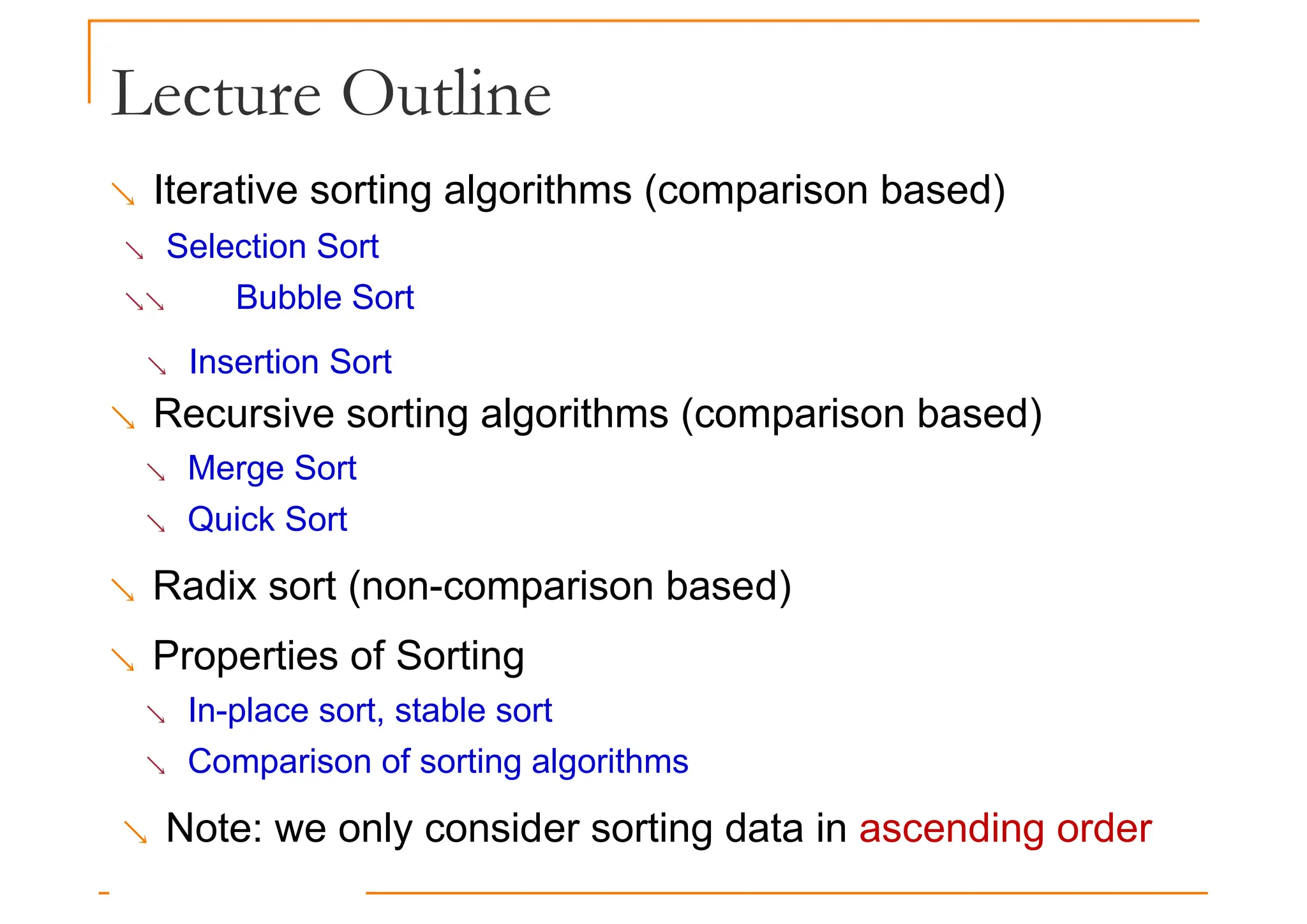
Lecture Outline
Iterativesorting algorithms (comparison based)
Selection Sort
Bubble Sort
Insertion Sort
Recursive sorting algorithms (comparison based)
Merge Sort
Quick Sort
Radix sort (non-comparison based)
Properties of Sorting
In-place sort, stable sort
Comparison of sorting algorithms
Note: we only consider sorting data in ascending order
3.
Why Study Sorting?
When an input is sorted, many problems become
easy (e.g. searching, min, max, k-th smallest)
Sorting has a variety of interesting algorithmic
solutions that embody many ideas
Comparison vs non-comparison based
Iterative
Recursive
Recursive
Divide-and-conquer
Best/worst/average-case bounds
Randomized algorithms
4.
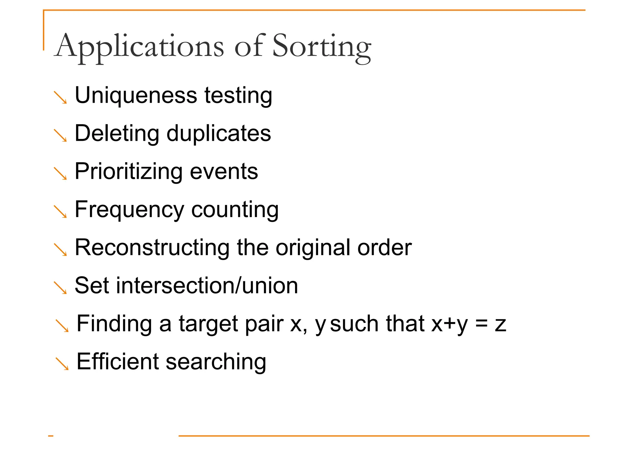
Applications of Sorting
Uniqueness testing
Deleting duplicates
Prioritizing events
Frequency counting
Reconstructing the original order
Set intersection/union
Finding a target pair x, ysuch that x+y = z
Efficient searching
Selection Sort: Idea
Given an array of nitems
1. Find the largest item x, in the range of [0…n−1]
2. Swap x with the (n−1)th item
3. Reduce n by 1 and go to Step 1
7.
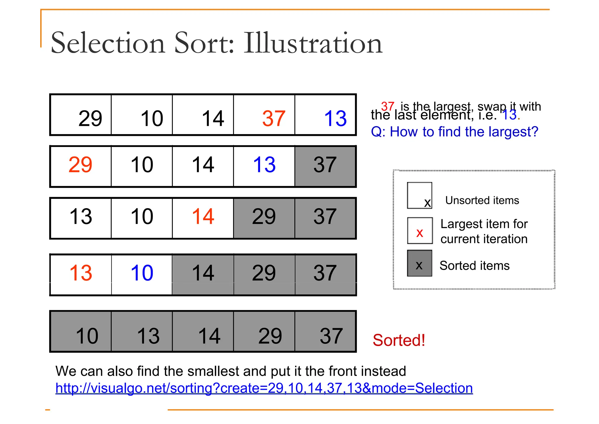
Selection Sort: Illustration
2910 14 37 13
37 is the largest, swap it with
the last element, i.e. 13.
Q: How to find the largest?
29 10 14 13 37
13 10 14 29 37
13 10 14 29 37
x
x
x Unsorted items
Largest item for
current iteration
Sorted items
13 10 14 29 37
10 13 14 29 37 Sorted!
We can also find the smallest and put it the front instead
http://visualgo.net/sorting?create=29,10,14,37,13&mode=Selection
8.
Selection Sort: Implementation
voidselectionSort(int a[], int n) {
for (int i = n-1; i >= 1; i--) {
int maxIdx = i;
for (int j = 0; j < i; j++)
Step 1:
for (int j = 0; j < i; j++) Search for
if (a[j] >= a[maxIdx])
maxIdx = j;
// swap routine is in STL <algorithm>
swap(a[i], a[maxIdx]);
}
}
Search for
maximum
element
Step 2:
Swap
8
} Swap
maximum
element
with the last
item i
9.
void selectionSort(int a[],int n) {
for (int i = n-1; i >= 1; i--) {
int maxIdx = i;
for (int j = 0; j < i; j++)
Selection Sort: Analysis
n−1
n−1
Number of times
executed
for (int j = 0; j < i; j++)
if (a[j] >= a[maxIdx])
maxIdx = j;
// swap routine is in STL <algorithm>
swap(a[i], a[maxIdx]);
}
}
(n−1)+(n−2)+…+1
= n(n−1)/2
n−1
} Total
• c1
and c2
are cost of statements in
outer and inner blocks
Total
= c1
(n−1) +
c2
*n*(n−1)/2
= O(n2)
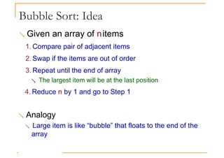
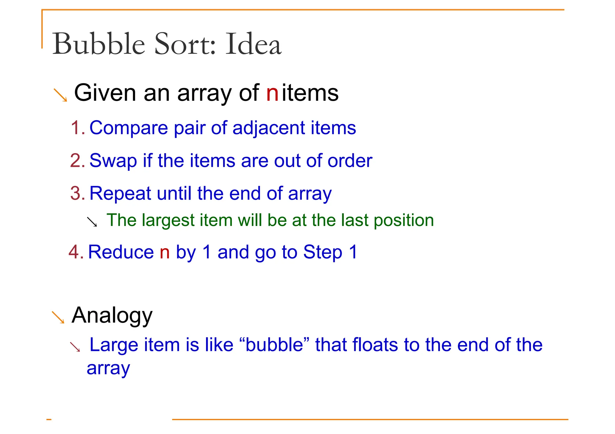
Bubble Sort: Idea
Given an array of nitems
1. Compare pair of adjacent items
2. Swap if the items are out of order
3. Repeat until the end of array
The largest item will be at the last position
4. Reduce n by 1 and go to Step 1
Analogy
Large item is like “bubble” that floats to the end of the
array
12.
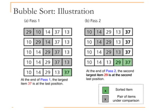
Bubble Sort: Illustration
Atthe end of Pass 2, the second
largest item 29 is at the second
At the end of Pass 1, the largest
item 37 is at the last position.
largest item 29 is at the second
last position.
x
x
Sorted Item
Pair of items
under comparison
13.
Bubble Sort: Implementation
voidbubbleSort(int a[], int n) {
for (int i = n-1; i >= 1; i--) {
for (int j = 1; j <= i; j++) {
if (a[j-1] > a[j])
swap(a[j], a[j-1]);
}
}
}
Step 2:
Swap if the
items are out
Compare
adjacent
pairs of
numbers
29 10 14 37 13
items are out
of order
http://visualgo.net/sorting?create=29,10,14,37,13&mode=Bubble
14.
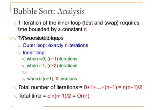
Bubble Sort: Analysis
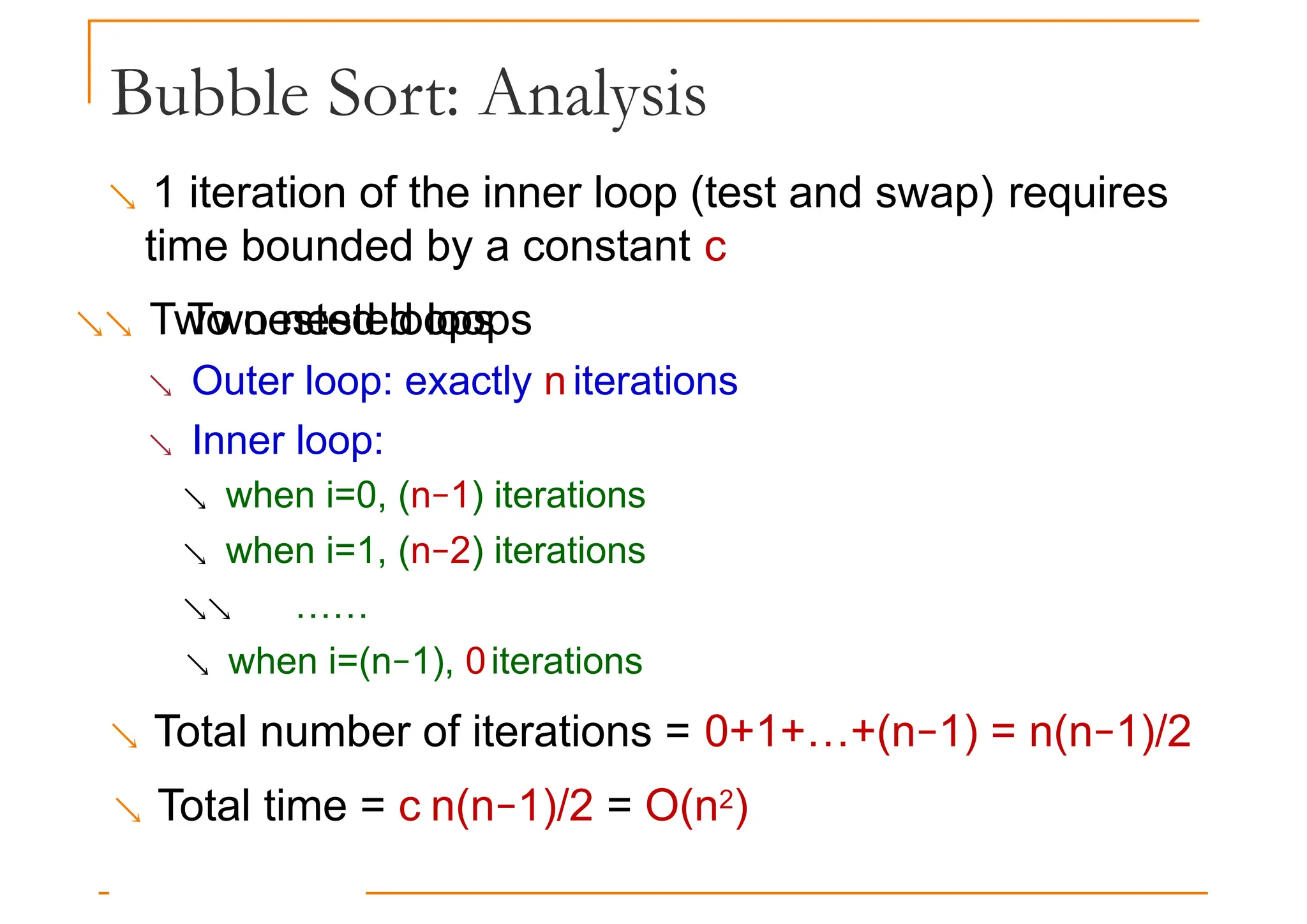
1 iteration of the inner loop (test and swap) requires
time bounded by a constant c
Two nested loops
Two nested loops
Outer loop: exactly n iterations
Inner loop:
when i=0, (n−1) iterations
when i=1, (n−2) iterations
……
when i=(n−1), 0iterations
Total number of iterations = 0+1+…+(n−1) = n(n−1)/2
Total time = c n(n−1)/2 = O(n2)
15.
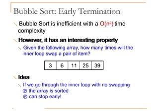
Bubble Sort: EarlyTermination
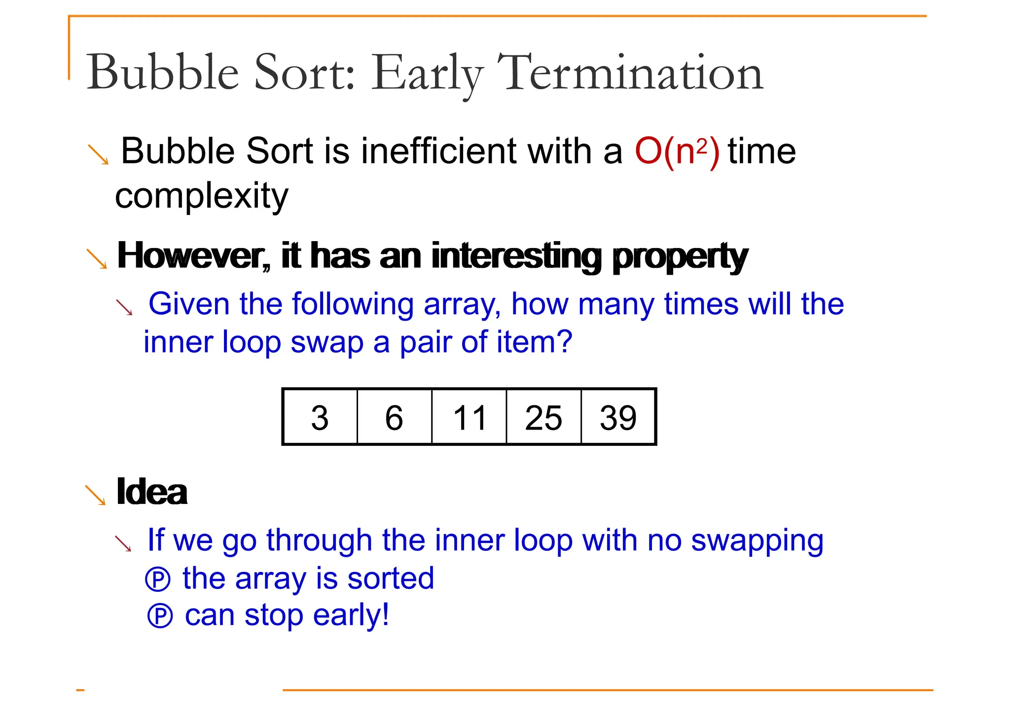
Bubble Sort is inefficient with a O(n2) time
complexity
However, it has an interesting property
However, it has an interesting property
Given the following array, how many times will the
inner loop swap a pair of item?
Idea
3 6 11 25 39
Idea
If we go through the inner loop with no swapping
the array is sorted
can stop early!
16.
Bubble Sort v2.0:Implementation
void bubbleSort2(int a[], int n) {
for (int i = n-1; i >= 1; i--) {
bool is_sorted = true;
for (int j = 1; j <= i; j++) {
Assume the array
is sorted before
the inner loop
for (int j = 1; j <= i; j++) {
if (a[j-1] > a[j]) {
swap(a[j], a[j-1]);
is_sorted = false;
}
} // end of inner loop
if (is_sorted) return;
the inner loop
Any swapping will
invalidate the
assumption
If the flag
if (is_sorted) return;
}
}
If the flag
remains true
after the inner
loop sorted!
17.
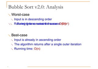
Bubble Sort v2.0:Analysis
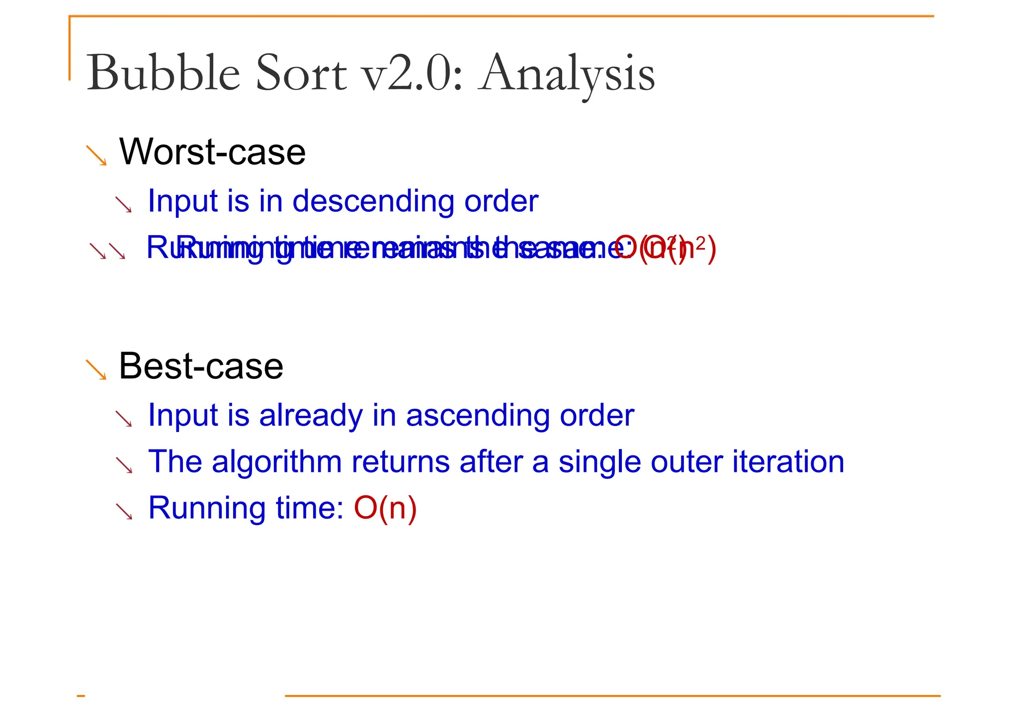
Worst-case
Input is in descending order
Running time remains the same: O(n2)
Running time remains the same: O(n2)
Best-case
Input is already in ascending order
The algorithm returns after a single outer iteration
Running time: O(n)
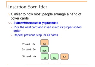
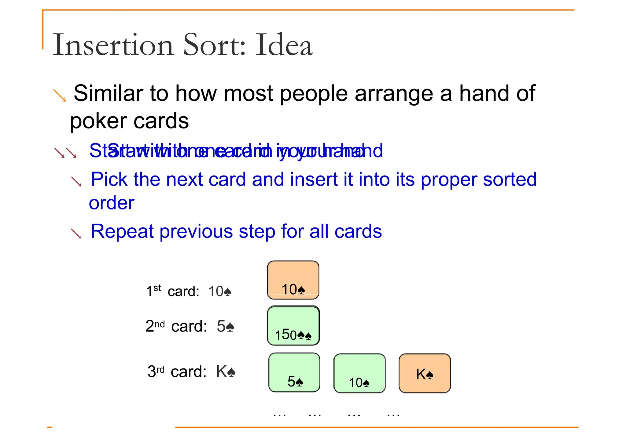
Insertion Sort: Idea
Similar to how most people arrange a hand of
poker cards
Start with one card in your hand
Start with one card in your hand
Pick the next card and insert it into its proper sorted
order
Repeat previous step for all cards
1st
card: 10♠ 10♠
K♠
150♠♠
5♠ 10♠
2nd card: 5♠
3rd card: K♠
… … … …
20.
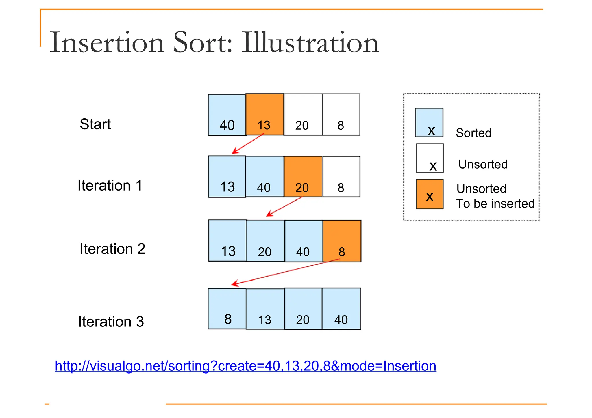
Insertion Sort: Illustration
Start40 13 20 8 x Sorted
x
x Unsorted
Unsorted
To be inserted
Iteration 1 13 40 20 8
Iteration 2 13 20 40 8
Iteration 3 8 13 20 40
http://visualgo.net/sorting?create=40,13,20,8&mode=Insertion
21.
Insertion Sort: Implementation
voidinsertionSort(int a[], int n) {
for (int i = 1; i < n; i++) {
int next = a[i];
next is the
item to be
inserted
int next = a[i];
int j;
for (j = i-1; j >= 0 && a[j] > next; j--)
a[j+1] = a[j];
a[j+1] = next;
}
inserted
Shift sorted
items to make
place for next
}
}
29 10 14 37 13
Insert next to
the correct
location
http://visualgo.net/sorting?create=29,10,14,37,13&mode=Insertion
22.
Insertion Sort: Analysis
Outer-loop executes (n−1) times
Number of times inner-loop is executed depends on
the input
the input
Best-case: the array is already sorted and
(a[j] > next) is always false
No shifting of data is necessary
Worst-case: the array is reversely sorted and
(a[j] > next) is always true
Insertion always occur at the front
Insertion always occur at the front
Therefore, the best-case time is O(n)
And the worst-case time is O(n2)
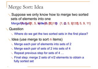
Merge Sort: Idea
Suppose we only know how to merge two sorted
sets of elements into one
Merge {1, 5, 9} with {2, 11} {1, 2, 5, 9, 11}
Merge {1, 5, 9} with {2, 11} {1, 2, 5, 9, 11}
Question
Where do we get the two sorted sets in the first place?
Idea (use merge to sort n items)
Merge each pair of elements into sets of 2
Merge each pair of sets of 2 into sets of 4
Repeat previous step for sets of 4 …
Final step: merge 2 sets of n/2 elements to obtain a
fully sorted set
25.
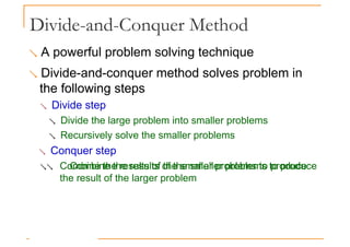
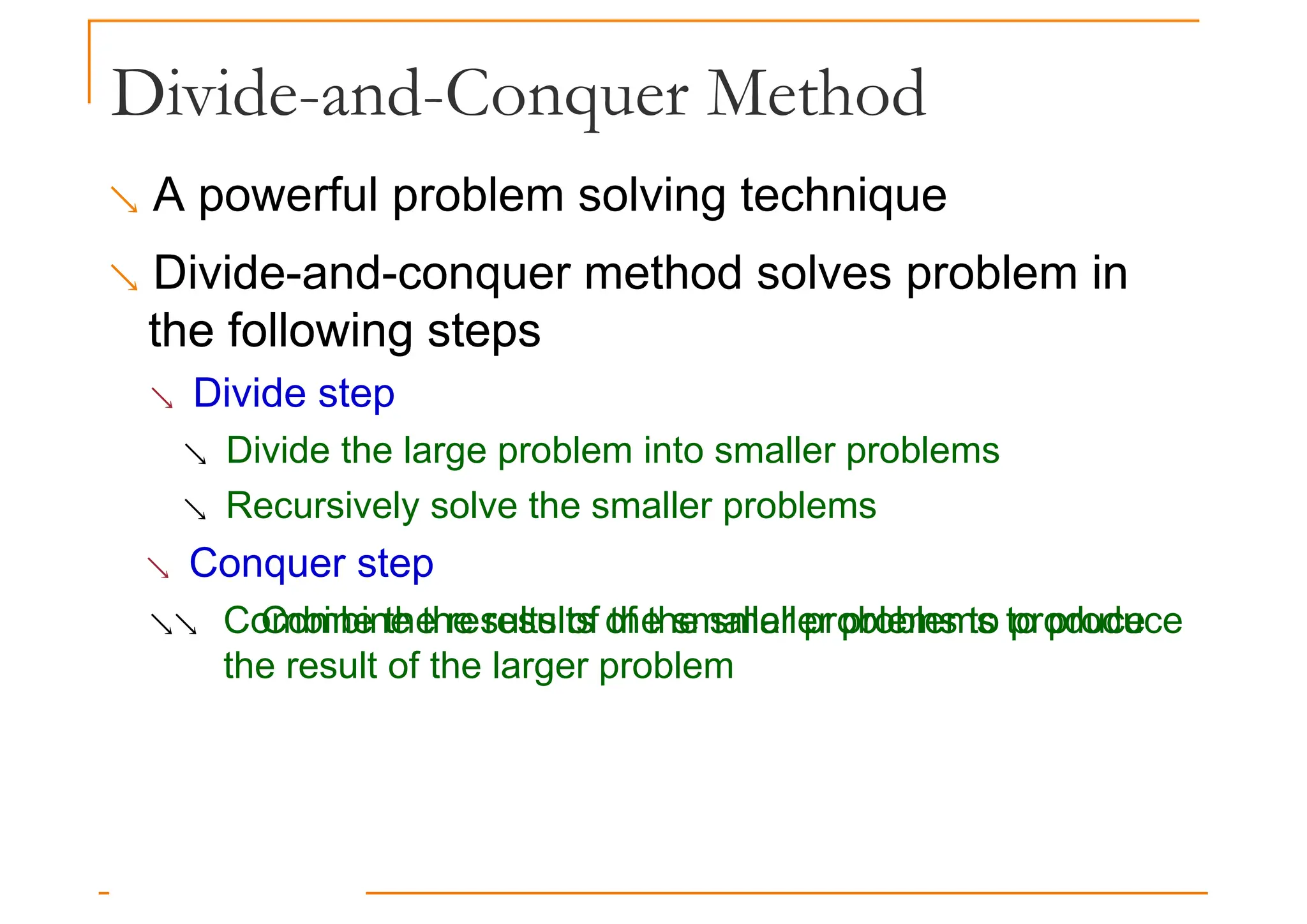
Divide-and-Conquer Method
Apowerful problem solving technique
Divide-and-conquer method solves problem in
the following steps
the following steps
Divide step
Divide the large problem into smaller problems
Recursively solve the smaller problems
Conquer step
Combine the results of the smaller problems to produce
Combine the results of the smaller problems to produce
the result of the larger problem
26.
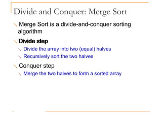
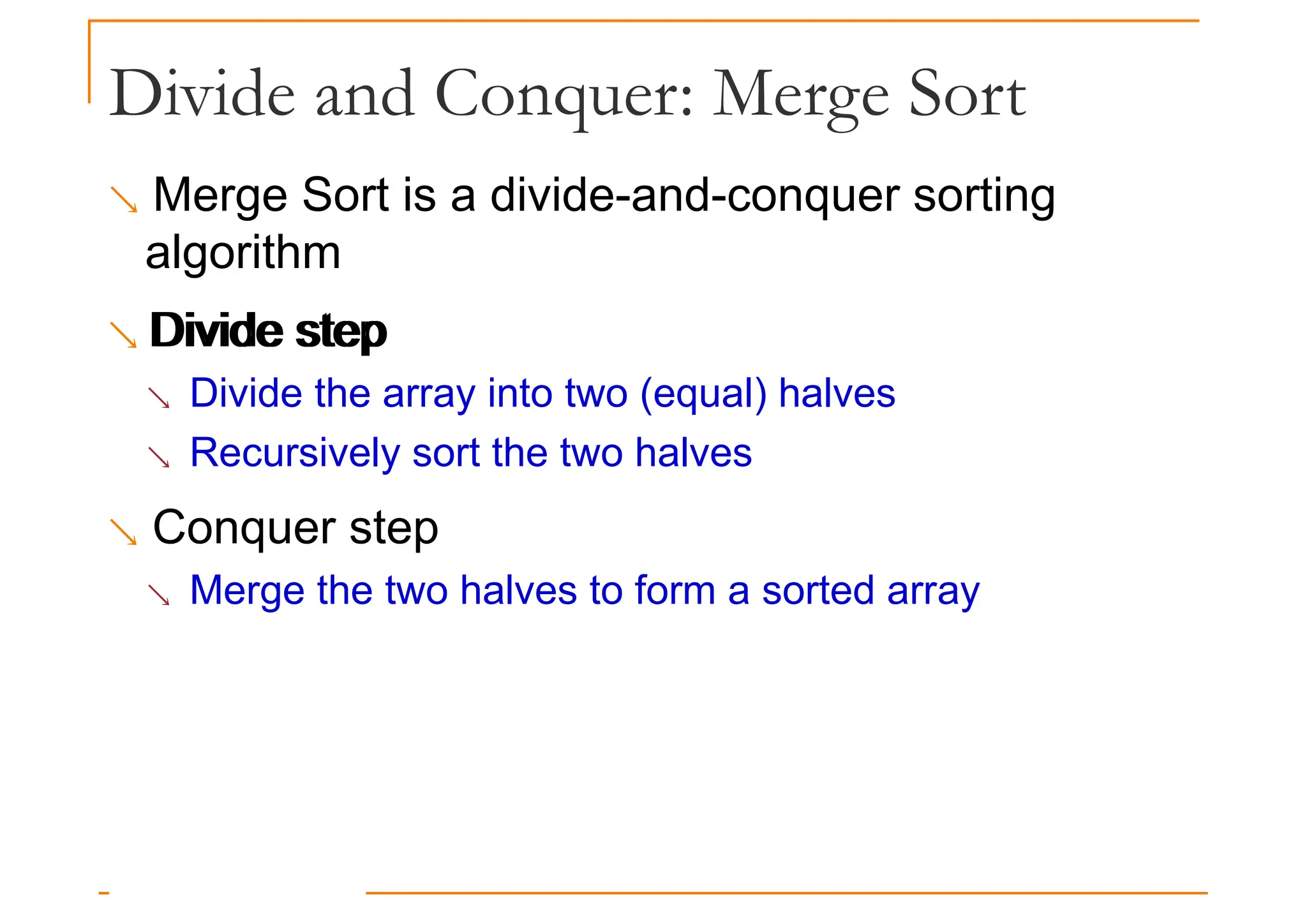
Divide and Conquer:Merge Sort
Merge Sort is a divide-and-conquer sorting
algorithm
Divide step
Divide step
Divide the array into two (equal) halves
Recursively sort the two halves
Conquer step
Merge the two halves to form a sorted array
27.
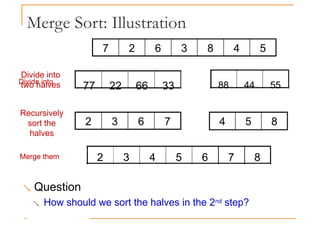
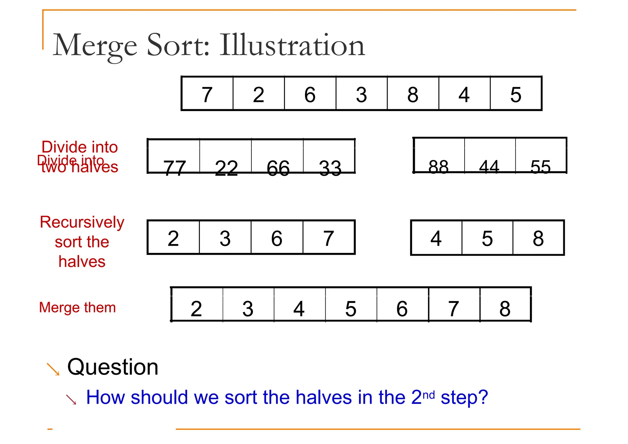
Merge Sort: Illustration
72 6 3 8 4 5
Divide into
77 22 66 33 88 44 55
2 3 6 7 4 5 8
Divide into
two halves
Recursively
sort the
halves
Merge them 2 3 4 5 6 7 8
Merge them 2 3 4 5 6 7 8
Question
How should we sort the halves in the 2nd step?
28.
Merge Sort: Implementation
voidmergeSort(int a[], int low, int high) {
if (low < high) {
int mid = (low+high) / 2;
mergeSort(a, low , mid );
Merge sort on
a[low...high]
mergeSort(a, low , mid ); Divide a[ ] into two
mergeSort(a, mid+1, high);
merge(a, low, mid, high);
}
Conquer: merge the
Function to merge
two sorted ha
a[low…mid] and
Divide a[ ] into two
halves and recursively
sort them
a[low…mid] and
a[mid+1…high] into
a[low…high]
Note
mergeSort() is a recursive function
low >= high is the base case, i.e. there is 0 or 1 item
Merge Sort: Merge
37 8
a[0..2] a[3..5] b[0..5]
2 4 5
3 7 8
3 7 8
3 7 8
3 7 8
2 4 5
2 4 5
2 4 5
2 4 5
2
2 3
2 3 4
2 3 4 5
3 7 8
3 7 8
2 4 5
2 4 5
2 3 4 5
2 3 4 5 7 8 x
x
x
Unmerged
items
Items used for
comparison
Merged items
Two sorted halves to be
merged
Merged result in a
temporary array
31.
Merge Sort: MergeImplementation
void merge(int a[], int low, int mid, int high) {
int n = high-low+1; b is a
temporary
PS: C++ STL <algorithm> has merge subroutine too
int* b = new int[n];
int left=low, right=mid+1, bIdx=0;
while (left <= mid && right <= high) {
if (a[left] <= a[right])
b[bIdx++] = a[left++];
else
Normal Merging
Where both
temporary
array to store
result
else
b[bIdx++] = a[right++];
}
// continue on next slide
Where both
halves have
unmerged items
32.
Merge Sort: MergeImplementation
// continued from previous slide
while (left <= mid) b[bIdx++] = a[left++];
while (right <= high) b[bIdx++] = a[right++];
for (int k = 0; k < n; k++)
a[low+k] = b[k];
delete [] b;
}
Merged result
are copied
back into a[]
Remaining
items are
copied into
b[]
}
Remember to free
allocated memory
Question
Why do we need a temporary array b[]?
33.
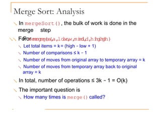
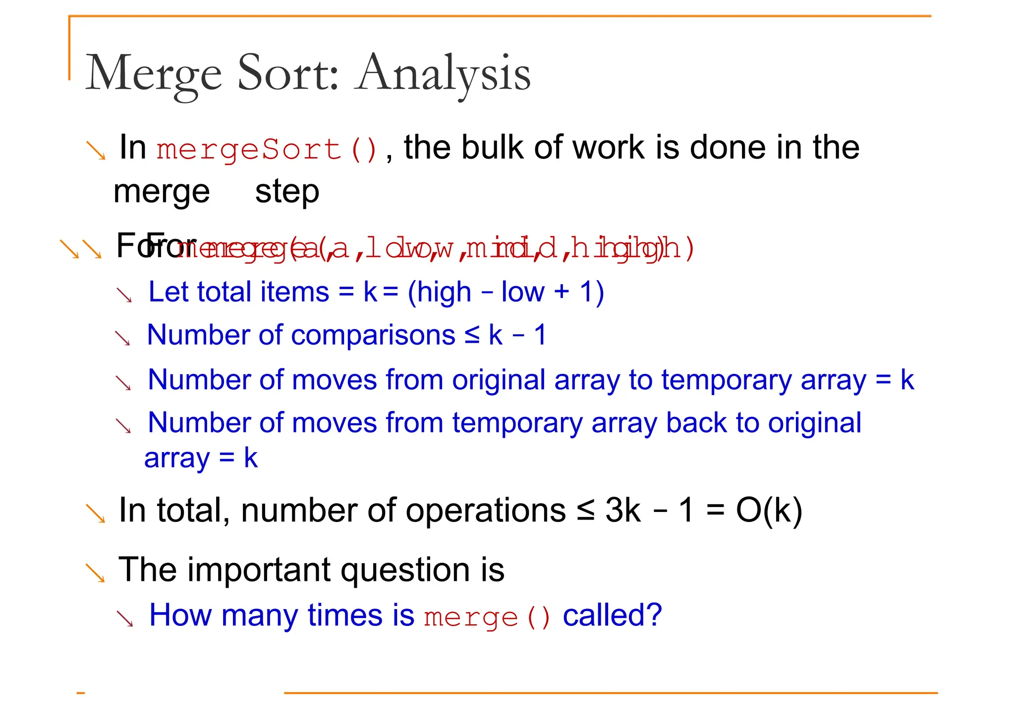
Merge Sort: Analysis
In mergeSort(), the bulk of work is done in the
merge step
For merge(a, low, mid, high)
For merge(a, low, mid, high)
Let total items = k = (high − low + 1)
Number of comparisons ≤ k − 1
Number of moves from original array to temporary array = k
Number of moves from temporary array back to original
array = k
In total, number of operations ≤ 3k − 1 = O(k)
The important question is
How many times is merge() called?
34.
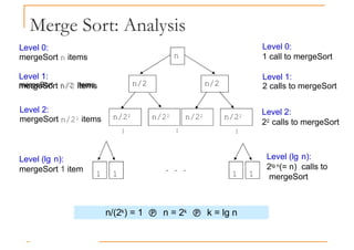
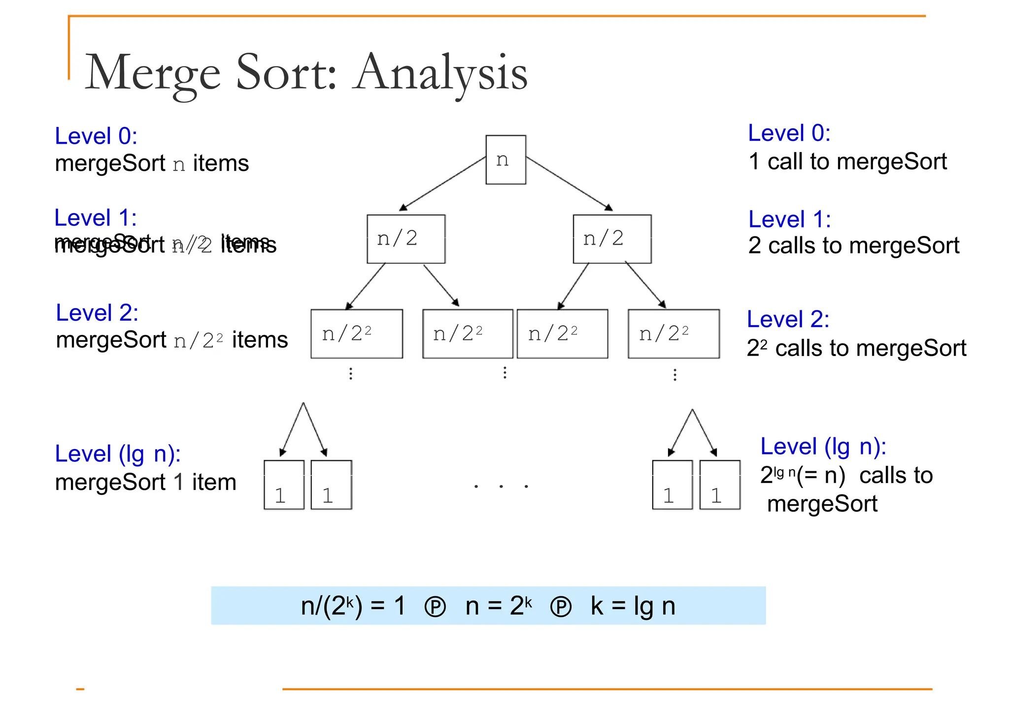
Merge Sort: Analysis
Level0:
mergeSort n items
Level 1:
mergeSort n/2 items
n
n/2 n/2
Level 0:
1 call to mergeSort
Level 1:
mergeSort n/2 items 2 calls to mergeSort
Level 2:
mergeSort n/22 items
Level (lg n):
mergeSort 1 item
n/2 n/2
n/22 n/22 n/22 n/22
…
1 1
. . .
1 1
Level 2:
22 calls to mergeSort
Level (lg n):
2lg n(= n) calls to
mergeSort
…
…
n/(2k) = 1 n = 2k k = lg n
35.
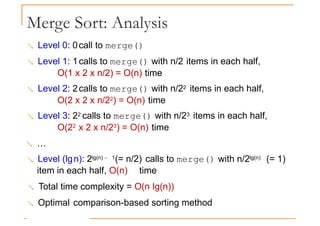
Merge Sort: Analysis
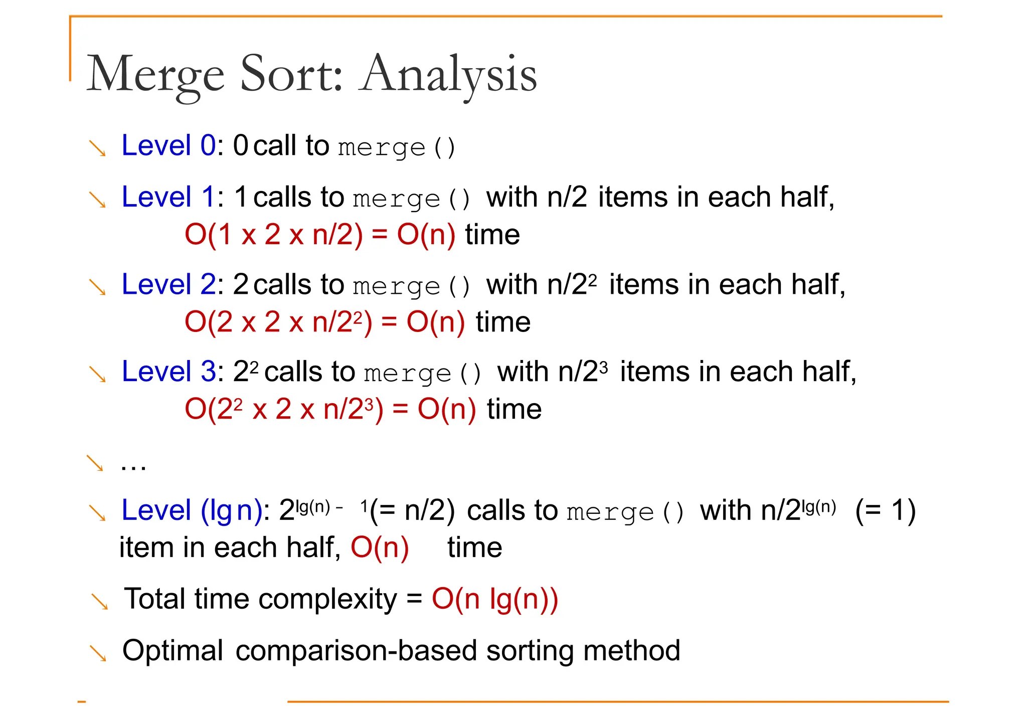
Level 0: 0call to merge()
Level 1: 1calls to merge() with n/2 items in each half,
O(1 x 2 x n/2) = O(n) time
O(1 x 2 x n/2) = O(n) time
Level 2: 2calls to merge() with n/22 items in each half,
O(2 x 2 x n/22) = O(n) time
Level 3: 22 calls to merge() with n/23 items in each half,
O(22 x 2 x n/23) = O(n) time
…
Level (lgn): 2lg(n) − 1(= n/2) calls to merge() with n/2lg(n) (= 1)
item in each half, O(n) time
Total time complexity = O(n lg(n))
Optimal comparison-based sorting method
36.
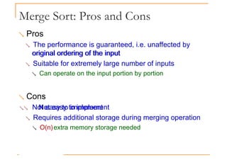
Merge Sort: Prosand Cons
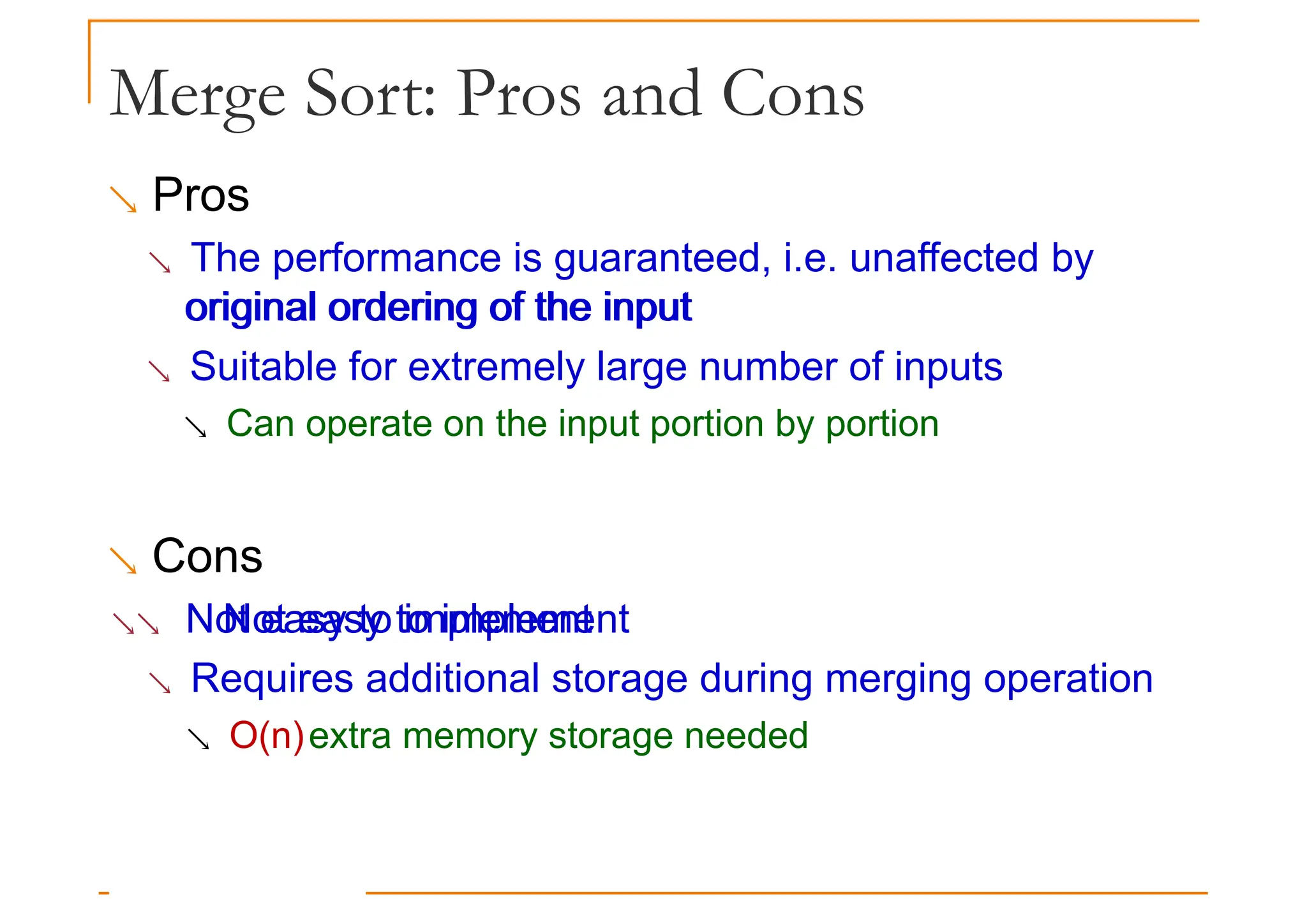
Pros
The performance is guaranteed, i.e. unaffected by
original ordering of the input
original ordering of the input
Suitable for extremely large number of inputs
Can operate on the input portion by portion
Cons
Not easy to implement
Not easy to implement
Requires additional storage during merging operation
O(n)extra memory storage needed
Quick Sort: Idea
Quick Sort is a divide-and-conquer algorithm
Divide step
Choose an item p (known as pivot) and partition the
Choose an item p (known as pivot) and partition the
items of a[i...j] into two parts
Items that are smaller than p
Items that are greater than or equal to p
Recursively sort the two parts
Conquer step
Do nothing!
Do nothing!
In comparison, Merge Sort spends most of the time
in conquer step but very little time in divide step
39.
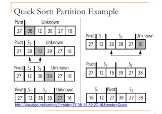
Quick Sort: DivideStep Example
27 38 12 39 27 1169
Pivot
Choose first
element as pivot
12 16 27 39 27 38
Pivot
12 16 27 27 38 39
Pivot
Partition a[] about
the pivot 27
Recursively sort
the two parts
the two parts 12 16 27 27 38 39
Notice anything special about the
position of pivot in the final
sorted items?
40.
Quick Sort: Implementation
voidquickSort(int a[], int low, int high) {
if (low < high) {
int pivotIdx = partition(a, low, high);
Partition
a[low...high]
and return the
quickSort(a, low, pivotIdx-1);
quickSort(a, pivotIdx+1, high);
}
}
and return the
index of the
pivot item
Recursively sort
the two portions
partition() splits a[low...high] into two portions
a[low ... pivot–1] and a[pivot+1 ... high]
Pivot item does not participate in any further sorting
41.
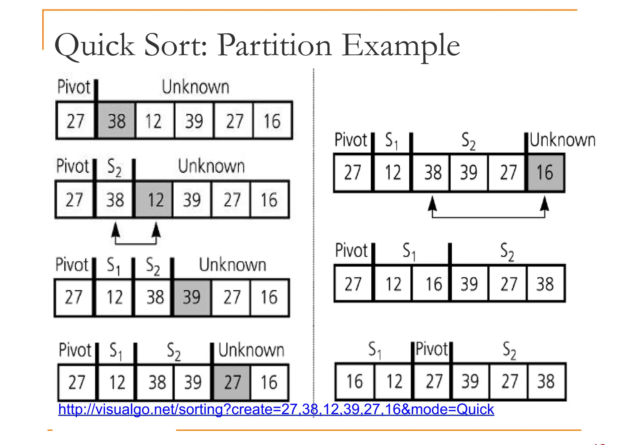
Quick Sort: PartitionAlgorithm
To partition a[i...j], we choose a[i] as the pivot p
Why choose a[i]? Are there other choices?
The remaining items (i.e. a[i+1...j]) are divided into 3
The remaining items (i.e. a[i+1...j]) are divided into 3
regions
S1= a[i+1...m] where items < p
S2= a[m+1...k-1] where item ≥ p
Unknown (unprocessed) = a[k...j], where items are yet to be
assigned to S1 or S2
p < p p ?
i m k j
S1 S2 Unknown
42.
Quick Sort: PartitionAlgorithm
Initially, regions S1 and S2 are empty
All items excluding p are in the unknown region
For each item a[k]in the unknown region
For each item a[k] in the unknown region
Compare a[k] with p
If a[k]>= p, put it into S2
Otherwise, put a[k]into S1
p ?
p ?
i k j
Unknown
43.
Quick Sort: PartitionAlgorithm
Case 1: if a[k]>= p
S1 S2
If a[k]=y p, p < p p ?
i m k j
x y
S1 S2
S1 S2
crement k p < p > p ?
i m k
44.
Quick Sort: PartitionAlgorithm
Case 2: if a[k]< p
If a[k]=y < p p < p x p y ?
S1 S2
If a[k]=y < p
p < p p ?
i m k j
Increment m x y
p < p y p x ?
p < p p ?
i m k j
x y
p < p p ?
i m k j
y x
Swap x and y
p < p p ?
i m k j
Increment k y x
45.
Quick Sort: PartitionImplementation
int partition(int a[], int i, int j) {
int p = a[i];
int m = i;
p is the pivot
S1 and S2 empty
PS: C++ STL <algorithm> has partition subroutine too
int m = i;
for (int k = i+1; k <= j; k++) {
if (a[k] < p) {
m++;
swap(a[k], a[m]);
}
else {
S1 and S2 empty
initially
Go through each
element in unknown
region
Case 1: Do nothing!
Case 2
}
}
swap(a[i], a[m]);
return m;
}
Case 1: Do nothing!
Swap pivot with a[m]
m is the index of pivot
Quick Sort: PartitionAnalysis
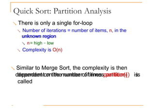
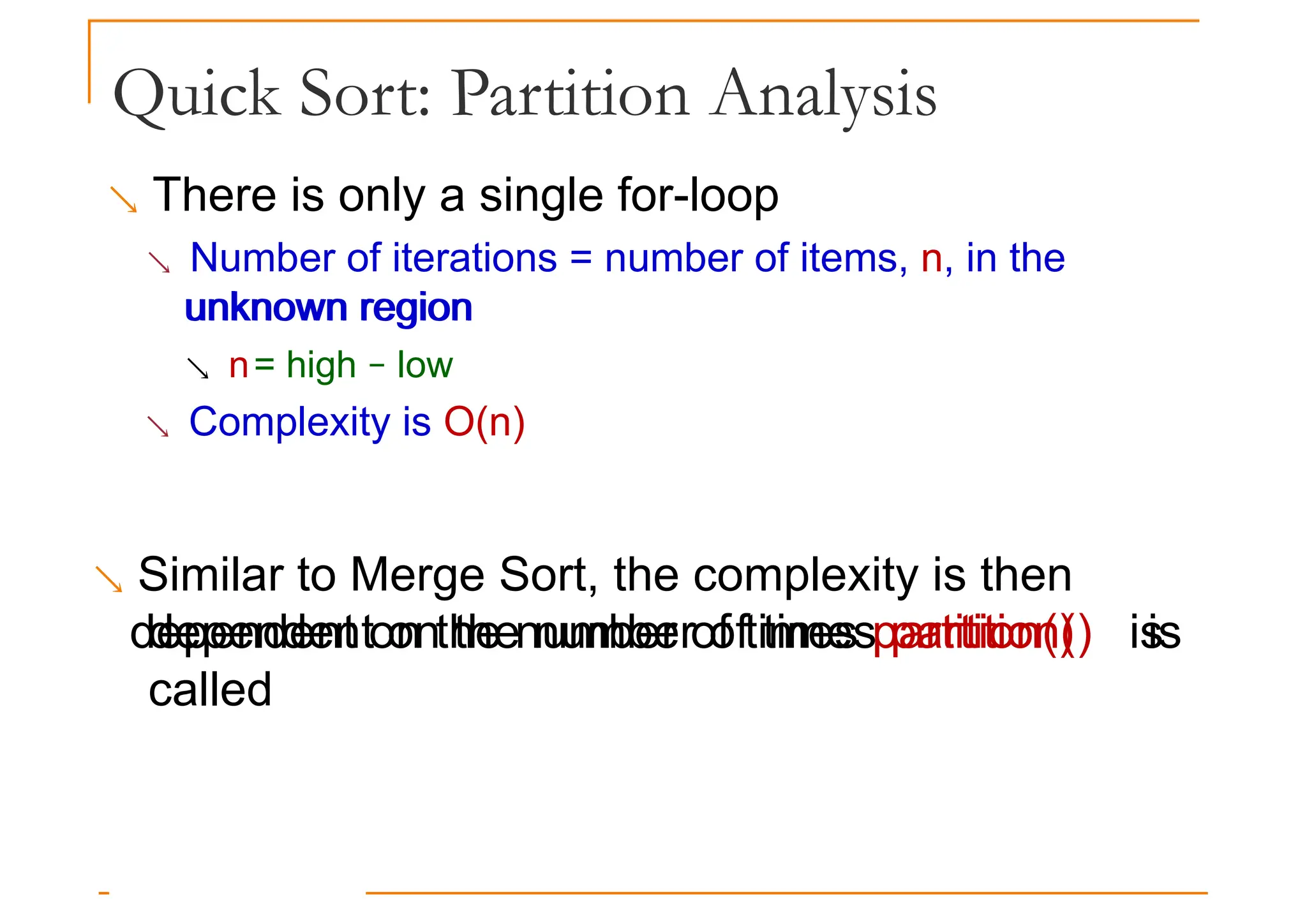
There is only a single for-loop
Number of iterations = number of items, n, in the
unknown region
unknown region
n= high − low
Complexity is O(n)
Similar to Merge Sort, the complexity is then
dependent on the number of times partition() is
dependent on the number of times partition() is
called
48.
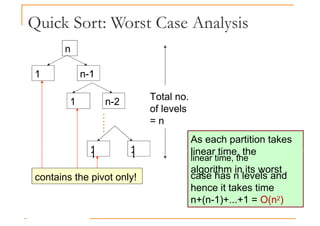
Quick Sort: WorstCase Analysis
When the array is already in ascending order
5 18 23 39 44 19
57
What is the pivot index returned by partition()?
5 18 23 39 44 19
57
S1 = a[i+1...m]
empty when m = i
S2 = a[m+1...j]
p = a[i]
What is the pivot index returned by partition()?
What is the effect of swap(a, i, m)?
S1is empty, while S2 contains every item except
the pivot
49.
Quick Sort: WorstCase Analysis
n
1 n-1
Total no.
of levels
= n
1 n-1
1 n-2
1 1
……
As each partition takes
linear time, the
1 1 linear time, the
algorithm in its worst
case has n levels and
hence it takes time
n+(n-1)+...+1 = O(n2)
contains the pivot only!
50.
Quick Sort: Best/AverageCase Analysis
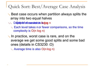
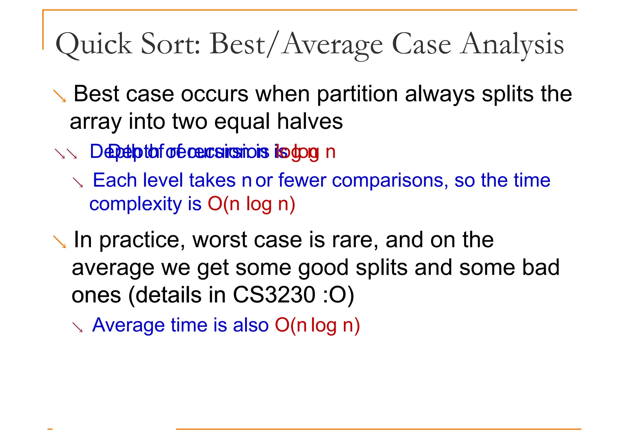
Best case occurs when partition always splits the
array into two equal halves
Depth of recursion is log n
Depth of recursion is log n
Each level takes n or fewer comparisons, so the time
complexity is O(n log n)
In practice, worst case is rare, and on the
average we get some good splits and some bad
ones (details in CS3230 :O)
ones (details in CS3230 :O)
Average time is also O(n log n)
51.
Lower Bound: Comparison-BasedSort
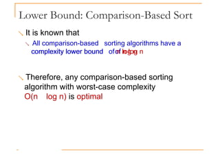
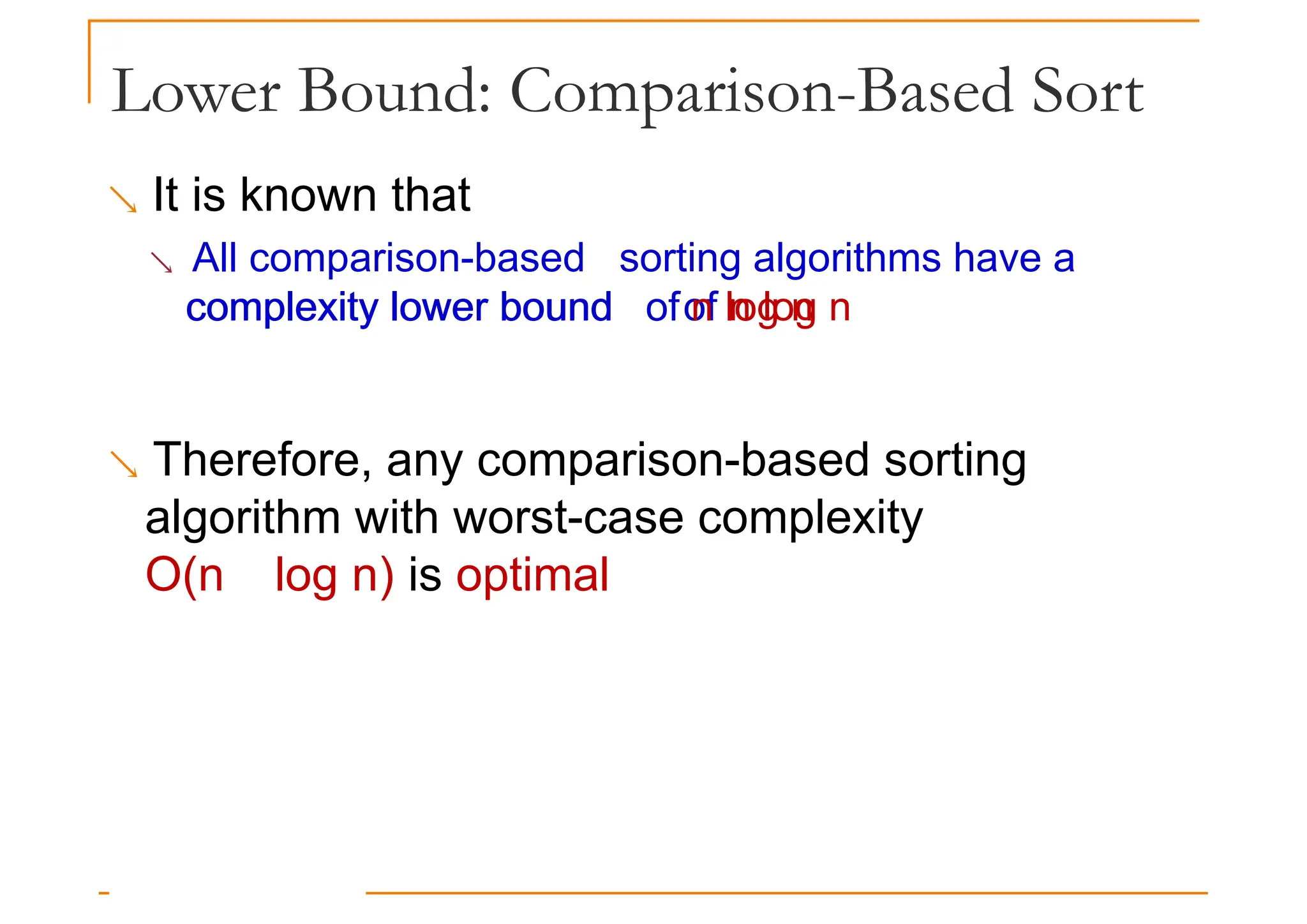
It is known that
All comparison-based sorting algorithms have a
complexity lower bound of n log n
complexity lower bound of n log n
Therefore, any comparison-based sorting
algorithm with worst-case complexity
O(n log n) is optimal
In-Place Sorting
Asort algorithm is said to be an in-place sort
If it requires only a constant amount (i.e. O(1)) of
extra space during the sorting process
extra space during the sorting process
Questions
Merge Sort is not in-place, why?
Is Quick Sort in-place?
Is Radix Sort in-place?
Is Radix Sort in-place?
[ CS1020E AY1617S1 Lecture 10 ]
54.
Stable Sorting
Asorting algorithm is stable if the relative order
of elements with the same key value is
preserved by the algorithm
preserved by the algorithm
Example application of stable sort
Assume that names have been sorted in alphabetical
order
Now, if this list is sorted again by tutorial group
Now, if this list is sorted again by tutorial group
number, a stable sort algorithm would ensure that all
students in the same tutorial groups still appear in
alphabetical order of their names
[ CS1020E AY1617S1 Lecture 10 ]
![Selection Sort: Idea
Given an array of nitems
1. Find the largest item x, in the range of [0…n−1]
2. Swap x with the (n−1)th item
3. Reduce n by 1 and go to Step 1](https://image.slidesharecdn.com/l9-sorting-251013171528-e58304c4/85/l9-Sorting-bubble-and-selection-sort-pptx-6-320.jpg)

![Selection Sort: Implementation
void selectionSort(int a[], int n) {
for (int i = n-1; i >= 1; i--) {
int maxIdx = i;
for (int j = 0; j < i; j++)
Step 1:
for (int j = 0; j < i; j++) Search for
if (a[j] >= a[maxIdx])
maxIdx = j;
// swap routine is in STL <algorithm>
swap(a[i], a[maxIdx]);
}
}
Search for
maximum
element
Step 2:
Swap
8
} Swap
maximum
element
with the last
item i](https://image.slidesharecdn.com/l9-sorting-251013171528-e58304c4/85/l9-Sorting-bubble-and-selection-sort-pptx-8-320.jpg)
![void selectionSort(int a[], int n) {
for (int i = n-1; i >= 1; i--) {
int maxIdx = i;
for (int j = 0; j < i; j++)
Selection Sort: Analysis
n−1
n−1
Number of times
executed
for (int j = 0; j < i; j++)
if (a[j] >= a[maxIdx])
maxIdx = j;
// swap routine is in STL <algorithm>
swap(a[i], a[maxIdx]);
}
}
(n−1)+(n−2)+…+1
= n(n−1)/2
n−1
} Total
• c1
and c2
are cost of statements in
outer and inner blocks
Total
= c1
(n−1) +
c2
*n*(n−1)/2
= O(n2)](https://image.slidesharecdn.com/l9-sorting-251013171528-e58304c4/85/l9-Sorting-bubble-and-selection-sort-pptx-9-320.jpg)
![Bubble Sort: Implementation
void bubbleSort(int a[], int n) {
for (int i = n-1; i >= 1; i--) {
for (int j = 1; j <= i; j++) {
if (a[j-1] > a[j])
swap(a[j], a[j-1]);
}
}
}
Step 2:
Swap if the
items are out
Compare
adjacent
pairs of
numbers
29 10 14 37 13
items are out
of order
http://visualgo.net/sorting?create=29,10,14,37,13&mode=Bubble](https://image.slidesharecdn.com/l9-sorting-251013171528-e58304c4/85/l9-Sorting-bubble-and-selection-sort-pptx-13-320.jpg)
![Bubble Sort v2.0: Implementation
void bubbleSort2(int a[], int n) {
for (int i = n-1; i >= 1; i--) {
bool is_sorted = true;
for (int j = 1; j <= i; j++) {
Assume the array
is sorted before
the inner loop
for (int j = 1; j <= i; j++) {
if (a[j-1] > a[j]) {
swap(a[j], a[j-1]);
is_sorted = false;
}
} // end of inner loop
if (is_sorted) return;
the inner loop
Any swapping will
invalidate the
assumption
If the flag
if (is_sorted) return;
}
}
If the flag
remains true
after the inner
loop sorted!](https://image.slidesharecdn.com/l9-sorting-251013171528-e58304c4/85/l9-Sorting-bubble-and-selection-sort-pptx-16-320.jpg)

![Insertion Sort: Implementation
void insertionSort(int a[], int n) {
for (int i = 1; i < n; i++) {
int next = a[i];
next is the
item to be
inserted
int next = a[i];
int j;
for (j = i-1; j >= 0 && a[j] > next; j--)
a[j+1] = a[j];
a[j+1] = next;
}
inserted
Shift sorted
items to make
place for next
}
}
29 10 14 37 13
Insert next to
the correct
location
http://visualgo.net/sorting?create=29,10,14,37,13&mode=Insertion](https://image.slidesharecdn.com/l9-sorting-251013171528-e58304c4/85/l9-Sorting-bubble-and-selection-sort-pptx-21-320.jpg)
![Insertion Sort: Analysis
Outer-loop executes (n−1) times
Number of times inner-loop is executed depends on
the input
the input
Best-case: the array is already sorted and
(a[j] > next) is always false
No shifting of data is necessary
Worst-case: the array is reversely sorted and
(a[j] > next) is always true
Insertion always occur at the front
Insertion always occur at the front
Therefore, the best-case time is O(n)
And the worst-case time is O(n2)](https://image.slidesharecdn.com/l9-sorting-251013171528-e58304c4/85/l9-Sorting-bubble-and-selection-sort-pptx-22-320.jpg)
![Merge Sort: Implementation
void mergeSort(int a[], int low, int high) {
if (low < high) {
int mid = (low+high) / 2;
mergeSort(a, low , mid );
Merge sort on
a[low...high]
mergeSort(a, low , mid ); Divide a[ ] into two
mergeSort(a, mid+1, high);
merge(a, low, mid, high);
}
Conquer: merge the
Function to merge
two sorted ha
a[low…mid] and
Divide a[ ] into two
halves and recursively
sort them
a[low…mid] and
a[mid+1…high] into
a[low…high]
Note
mergeSort() is a recursive function
low >= high is the base case, i.e. there is 0 or 1 item](https://image.slidesharecdn.com/l9-sorting-251013171528-e58304c4/85/l9-Sorting-bubble-and-selection-sort-pptx-28-320.jpg)
![Merge Sort: Example
mergeSort(a[low…mid])
mergeSort(a[mid+1…high])
merge(a[low..mid],
a[mid+1..high])
38 16 27 39 12 27
38 16 27 39 12 27 a[mid+1..high])
38 16
38 16
16 38
27
39 12
39 12
12 39
27
Divide Phase
Recursive call to
mergeSort()
Conquer Phase
16 27 38 12 27 39
12 16 27 27 38 39
Conquer Phase
Merge steps
http://visualgo.net/sorting?create=38,16,27,39,12,27&mode=Merge](https://image.slidesharecdn.com/l9-sorting-251013171528-e58304c4/85/l9-Sorting-bubble-and-selection-sort-pptx-29-320.jpg)
![Merge Sort: Merge
3 7 8
a[0..2] a[3..5] b[0..5]
2 4 5
3 7 8
3 7 8
3 7 8
3 7 8
2 4 5
2 4 5
2 4 5
2 4 5
2
2 3
2 3 4
2 3 4 5
3 7 8
3 7 8
2 4 5
2 4 5
2 3 4 5
2 3 4 5 7 8 x
x
x
Unmerged
items
Items used for
comparison
Merged items
Two sorted halves to be
merged
Merged result in a
temporary array](https://image.slidesharecdn.com/l9-sorting-251013171528-e58304c4/85/l9-Sorting-bubble-and-selection-sort-pptx-30-320.jpg)
![Merge Sort: Merge Implementation
void merge(int a[], int low, int mid, int high) {
int n = high-low+1; b is a
temporary
PS: C++ STL <algorithm> has merge subroutine too
int* b = new int[n];
int left=low, right=mid+1, bIdx=0;
while (left <= mid && right <= high) {
if (a[left] <= a[right])
b[bIdx++] = a[left++];
else
Normal Merging
Where both
temporary
array to store
result
else
b[bIdx++] = a[right++];
}
// continue on next slide
Where both
halves have
unmerged items](https://image.slidesharecdn.com/l9-sorting-251013171528-e58304c4/85/l9-Sorting-bubble-and-selection-sort-pptx-31-320.jpg)
![Merge Sort: Merge Implementation
// continued from previous slide
while (left <= mid) b[bIdx++] = a[left++];
while (right <= high) b[bIdx++] = a[right++];
for (int k = 0; k < n; k++)
a[low+k] = b[k];
delete [] b;
}
Merged result
are copied
back into a[]
Remaining
items are
copied into
b[]
}
Remember to free
allocated memory
Question
Why do we need a temporary array b[]?](https://image.slidesharecdn.com/l9-sorting-251013171528-e58304c4/85/l9-Sorting-bubble-and-selection-sort-pptx-32-320.jpg)
![Quick Sort: Idea
Quick Sort is a divide-and-conquer algorithm
Divide step
Choose an item p (known as pivot) and partition the
Choose an item p (known as pivot) and partition the
items of a[i...j] into two parts
Items that are smaller than p
Items that are greater than or equal to p
Recursively sort the two parts
Conquer step
Do nothing!
Do nothing!
In comparison, Merge Sort spends most of the time
in conquer step but very little time in divide step](https://image.slidesharecdn.com/l9-sorting-251013171528-e58304c4/85/l9-Sorting-bubble-and-selection-sort-pptx-38-320.jpg)
![Quick Sort: Divide Step Example
27 38 12 39 27 1169
Pivot
Choose first
element as pivot
12 16 27 39 27 38
Pivot
12 16 27 27 38 39
Pivot
Partition a[] about
the pivot 27
Recursively sort
the two parts
the two parts 12 16 27 27 38 39
Notice anything special about the
position of pivot in the final
sorted items?](https://image.slidesharecdn.com/l9-sorting-251013171528-e58304c4/85/l9-Sorting-bubble-and-selection-sort-pptx-39-320.jpg)
![Quick Sort: Implementation
void quickSort(int a[], int low, int high) {
if (low < high) {
int pivotIdx = partition(a, low, high);
Partition
a[low...high]
and return the
quickSort(a, low, pivotIdx-1);
quickSort(a, pivotIdx+1, high);
}
}
and return the
index of the
pivot item
Recursively sort
the two portions
partition() splits a[low...high] into two portions
a[low ... pivot–1] and a[pivot+1 ... high]
Pivot item does not participate in any further sorting](https://image.slidesharecdn.com/l9-sorting-251013171528-e58304c4/85/l9-Sorting-bubble-and-selection-sort-pptx-40-320.jpg)
![Quick Sort: Partition Algorithm
To partition a[i...j], we choose a[i] as the pivot p
Why choose a[i]? Are there other choices?
The remaining items (i.e. a[i+1...j]) are divided into 3
The remaining items (i.e. a[i+1...j]) are divided into 3
regions
S1= a[i+1...m] where items < p
S2= a[m+1...k-1] where item ≥ p
Unknown (unprocessed) = a[k...j], where items are yet to be
assigned to S1 or S2
p < p p ?
i m k j
S1 S2 Unknown](https://image.slidesharecdn.com/l9-sorting-251013171528-e58304c4/85/l9-Sorting-bubble-and-selection-sort-pptx-41-320.jpg)
![Quick Sort: Partition Algorithm
Initially, regions S1 and S2 are empty
All items excluding p are in the unknown region
For each item a[k]in the unknown region
For each item a[k] in the unknown region
Compare a[k] with p
If a[k]>= p, put it into S2
Otherwise, put a[k]into S1
p ?
p ?
i k j
Unknown](https://image.slidesharecdn.com/l9-sorting-251013171528-e58304c4/85/l9-Sorting-bubble-and-selection-sort-pptx-42-320.jpg)
![Quick Sort: Partition Algorithm
Case 1: if a[k]>= p
S1 S2
If a[k]=y p, p < p p ?
i m k j
x y
S1 S2
S1 S2
crement k p < p > p ?
i m k](https://image.slidesharecdn.com/l9-sorting-251013171528-e58304c4/85/l9-Sorting-bubble-and-selection-sort-pptx-43-320.jpg)
![Quick Sort: Partition Algorithm
Case 2: if a[k]< p
If a[k]=y < p p < p x p y ?
S1 S2
If a[k]=y < p
p < p p ?
i m k j
Increment m x y
p < p y p x ?
p < p p ?
i m k j
x y
p < p p ?
i m k j
y x
Swap x and y
p < p p ?
i m k j
Increment k y x](https://image.slidesharecdn.com/l9-sorting-251013171528-e58304c4/85/l9-Sorting-bubble-and-selection-sort-pptx-44-320.jpg)
![Quick Sort: Partition Implementation
int partition(int a[], int i, int j) {
int p = a[i];
int m = i;
p is the pivot
S1 and S2 empty
PS: C++ STL <algorithm> has partition subroutine too
int m = i;
for (int k = i+1; k <= j; k++) {
if (a[k] < p) {
m++;
swap(a[k], a[m]);
}
else {
S1 and S2 empty
initially
Go through each
element in unknown
region
Case 1: Do nothing!
Case 2
}
}
swap(a[i], a[m]);
return m;
}
Case 1: Do nothing!
Swap pivot with a[m]
m is the index of pivot](https://image.slidesharecdn.com/l9-sorting-251013171528-e58304c4/85/l9-Sorting-bubble-and-selection-sort-pptx-45-320.jpg)
![Quick Sort: Worst Case Analysis
When the array is already in ascending order
5 18 23 39 44 19
57
What is the pivot index returned by partition()?
5 18 23 39 44 19
57
S1 = a[i+1...m]
empty when m = i
S2 = a[m+1...j]
p = a[i]
What is the pivot index returned by partition()?
What is the effect of swap(a, i, m)?
S1is empty, while S2 contains every item except
the pivot](https://image.slidesharecdn.com/l9-sorting-251013171528-e58304c4/85/l9-Sorting-bubble-and-selection-sort-pptx-48-320.jpg)
![In-Place Sorting
A sort algorithm is said to be an in-place sort
If it requires only a constant amount (i.e. O(1)) of
extra space during the sorting process
extra space during the sorting process
Questions
Merge Sort is not in-place, why?
Is Quick Sort in-place?
Is Radix Sort in-place?
Is Radix Sort in-place?
[ CS1020E AY1617S1 Lecture 10 ]](https://image.slidesharecdn.com/l9-sorting-251013171528-e58304c4/85/l9-Sorting-bubble-and-selection-sort-pptx-53-320.jpg)
![Stable Sorting
A sorting algorithm is stable if the relative order
of elements with the same key value is
preserved by the algorithm
preserved by the algorithm
Example application of stable sort
Assume that names have been sorted in alphabetical
order
Now, if this list is sorted again by tutorial group
Now, if this list is sorted again by tutorial group
number, a stable sort algorithm would ensure that all
students in the same tutorial groups still appear in
alphabetical order of their names
[ CS1020E AY1617S1 Lecture 10 ]](https://image.slidesharecdn.com/l9-sorting-251013171528-e58304c4/85/l9-Sorting-bubble-and-selection-sort-pptx-54-320.jpg)
![Non-Stable Sort
Selection Sort
1285 5a
4746 602 5b
(8356)
1285 5 5 602 (4746 8356)
1285 5a
5b
602 (4746 8356)
602 5a
5b
(1285 4746 8356)
5b
5a
(602 1285 4746 8356)
Quick Sort
1285 5 150 4746 602 5 8356 (pivot=1285)
1285 5a
150 4746 602 5b
8356 (pivot=1285)
1285 (5a
150 602 5b
) (4746 8356)
5b
5a
150 602 1285 4746 8356
[ CS1020E AY1617S1 Lecture 10 ]](https://image.slidesharecdn.com/l9-sorting-251013171528-e58304c4/85/l9-Sorting-bubble-and-selection-sort-pptx-55-320.jpg)
![Sorting Algorithms: Summary
Worst
Case
Best
Case
In-place? Stable?
Selection
Sort
O(n
2
) O(n2
) Yes No
Sort
Insertion
Sort
O(n 2
) O(n) Yes Yes
Bubble Sort O(n2
) O(n2
) Yes Yes
Bubble Sort 2 O(n2
) O(n) Yes Yes
[ CS1020E AY1617S1 Lecture 10 ]
Merge Sort O(n lg n) O(n lg n) No Yes
Quick Sort O(n2
) O(n lg n) Yes No](https://image.slidesharecdn.com/l9-sorting-251013171528-e58304c4/85/l9-Sorting-bubble-and-selection-sort-pptx-56-320.jpg)
![Summary
Comparison-Based Sorting Algorithms
Iterative Sorting
Selection Sort
Bubble Sort
Insertion Sort
Recursive Sorting
Merge Sort
Quick Sort
Non-Comparison-Based Sorting Algorithms
Non-Comparison-Based Sorting Algorithms
Radix Sort
Properties of Sorting Algorithms
In-Place
Stable
[ CS1020E AY1617S1 Lecture 10 ]](https://image.slidesharecdn.com/l9-sorting-251013171528-e58304c4/85/l9-Sorting-bubble-and-selection-sort-pptx-57-320.jpg)

![Selection Sort: Idea
Given an array of nitems
1. Find the largest item x, in the range of [0…n−1]
2. Swap x with the (n−1)th item
3. Reduce n by 1 and go to Step 1](https://image.slidesharecdn.com/l9-sorting-251013171528-e58304c4/75/l9-Sorting-bubble-and-selection-sort-pptx-6-2048.jpg)
![Selection Sort: Implementation
void selectionSort(int a[], int n) {
for (int i = n-1; i >= 1; i--) {
int maxIdx = i;
for (int j = 0; j < i; j++)
Step 1:
for (int j = 0; j < i; j++) Search for
if (a[j] >= a[maxIdx])
maxIdx = j;
// swap routine is in STL <algorithm>
swap(a[i], a[maxIdx]);
}
}
Search for
maximum
element
Step 2:
Swap
8
} Swap
maximum
element
with the last
item i](https://image.slidesharecdn.com/l9-sorting-251013171528-e58304c4/75/l9-Sorting-bubble-and-selection-sort-pptx-8-2048.jpg)
![void selectionSort(int a[], int n) {
for (int i = n-1; i >= 1; i--) {
int maxIdx = i;
for (int j = 0; j < i; j++)
Selection Sort: Analysis
n−1
n−1
Number of times
executed
for (int j = 0; j < i; j++)
if (a[j] >= a[maxIdx])
maxIdx = j;
// swap routine is in STL <algorithm>
swap(a[i], a[maxIdx]);
}
}
(n−1)+(n−2)+…+1
= n(n−1)/2
n−1
} Total
• c1
and c2
are cost of statements in
outer and inner blocks
Total
= c1
(n−1) +
c2
*n*(n−1)/2
= O(n2)](https://image.slidesharecdn.com/l9-sorting-251013171528-e58304c4/75/l9-Sorting-bubble-and-selection-sort-pptx-9-2048.jpg)

![Bubble Sort: Implementation
void bubbleSort(int a[], int n) {
for (int i = n-1; i >= 1; i--) {
for (int j = 1; j <= i; j++) {
if (a[j-1] > a[j])
swap(a[j], a[j-1]);
}
}
}
Step 2:
Swap if the
items are out
Compare
adjacent
pairs of
numbers
29 10 14 37 13
items are out
of order
http://visualgo.net/sorting?create=29,10,14,37,13&mode=Bubble](https://image.slidesharecdn.com/l9-sorting-251013171528-e58304c4/75/l9-Sorting-bubble-and-selection-sort-pptx-13-2048.jpg)
![Bubble Sort v2.0: Implementation
void bubbleSort2(int a[], int n) {
for (int i = n-1; i >= 1; i--) {
bool is_sorted = true;
for (int j = 1; j <= i; j++) {
Assume the array
is sorted before
the inner loop
for (int j = 1; j <= i; j++) {
if (a[j-1] > a[j]) {
swap(a[j], a[j-1]);
is_sorted = false;
}
} // end of inner loop
if (is_sorted) return;
the inner loop
Any swapping will
invalidate the
assumption
If the flag
if (is_sorted) return;
}
}
If the flag
remains true
after the inner
loop sorted!](https://image.slidesharecdn.com/l9-sorting-251013171528-e58304c4/75/l9-Sorting-bubble-and-selection-sort-pptx-16-2048.jpg)
![Insertion Sort: Implementation
void insertionSort(int a[], int n) {
for (int i = 1; i < n; i++) {
int next = a[i];
next is the
item to be
inserted
int next = a[i];
int j;
for (j = i-1; j >= 0 && a[j] > next; j--)
a[j+1] = a[j];
a[j+1] = next;
}
inserted
Shift sorted
items to make
place for next
}
}
29 10 14 37 13
Insert next to
the correct
location
http://visualgo.net/sorting?create=29,10,14,37,13&mode=Insertion](https://image.slidesharecdn.com/l9-sorting-251013171528-e58304c4/75/l9-Sorting-bubble-and-selection-sort-pptx-21-2048.jpg)
![Insertion Sort: Analysis
Outer-loop executes (n−1) times
Number of times inner-loop is executed depends on
the input
the input
Best-case: the array is already sorted and
(a[j] > next) is always false
No shifting of data is necessary
Worst-case: the array is reversely sorted and
(a[j] > next) is always true
Insertion always occur at the front
Insertion always occur at the front
Therefore, the best-case time is O(n)
And the worst-case time is O(n2)](https://image.slidesharecdn.com/l9-sorting-251013171528-e58304c4/75/l9-Sorting-bubble-and-selection-sort-pptx-22-2048.jpg)

![Merge Sort: Implementation
void mergeSort(int a[], int low, int high) {
if (low < high) {
int mid = (low+high) / 2;
mergeSort(a, low , mid );
Merge sort on
a[low...high]
mergeSort(a, low , mid ); Divide a[ ] into two
mergeSort(a, mid+1, high);
merge(a, low, mid, high);
}
Conquer: merge the
Function to merge
two sorted ha
a[low…mid] and
Divide a[ ] into two
halves and recursively
sort them
a[low…mid] and
a[mid+1…high] into
a[low…high]
Note
mergeSort() is a recursive function
low >= high is the base case, i.e. there is 0 or 1 item](https://image.slidesharecdn.com/l9-sorting-251013171528-e58304c4/75/l9-Sorting-bubble-and-selection-sort-pptx-28-2048.jpg)
![Merge Sort: Example
mergeSort(a[low…mid])
mergeSort(a[mid+1…high])
merge(a[low..mid],
a[mid+1..high])
38 16 27 39 12 27
38 16 27 39 12 27 a[mid+1..high])
38 16
38 16
16 38
27
39 12
39 12
12 39
27
Divide Phase
Recursive call to
mergeSort()
Conquer Phase
16 27 38 12 27 39
12 16 27 27 38 39
Conquer Phase
Merge steps
http://visualgo.net/sorting?create=38,16,27,39,12,27&mode=Merge](https://image.slidesharecdn.com/l9-sorting-251013171528-e58304c4/75/l9-Sorting-bubble-and-selection-sort-pptx-29-2048.jpg)
![Merge Sort: Merge
3 7 8
a[0..2] a[3..5] b[0..5]
2 4 5
3 7 8
3 7 8
3 7 8
3 7 8
2 4 5
2 4 5
2 4 5
2 4 5
2
2 3
2 3 4
2 3 4 5
3 7 8
3 7 8
2 4 5
2 4 5
2 3 4 5
2 3 4 5 7 8 x
x
x
Unmerged
items
Items used for
comparison
Merged items
Two sorted halves to be
merged
Merged result in a
temporary array](https://image.slidesharecdn.com/l9-sorting-251013171528-e58304c4/75/l9-Sorting-bubble-and-selection-sort-pptx-30-2048.jpg)
![Merge Sort: Merge Implementation
void merge(int a[], int low, int mid, int high) {
int n = high-low+1; b is a
temporary
PS: C++ STL <algorithm> has merge subroutine too
int* b = new int[n];
int left=low, right=mid+1, bIdx=0;
while (left <= mid && right <= high) {
if (a[left] <= a[right])
b[bIdx++] = a[left++];
else
Normal Merging
Where both
temporary
array to store
result
else
b[bIdx++] = a[right++];
}
// continue on next slide
Where both
halves have
unmerged items](https://image.slidesharecdn.com/l9-sorting-251013171528-e58304c4/75/l9-Sorting-bubble-and-selection-sort-pptx-31-2048.jpg)
![Merge Sort: Merge Implementation
// continued from previous slide
while (left <= mid) b[bIdx++] = a[left++];
while (right <= high) b[bIdx++] = a[right++];
for (int k = 0; k < n; k++)
a[low+k] = b[k];
delete [] b;
}
Merged result
are copied
back into a[]
Remaining
items are
copied into
b[]
}
Remember to free
allocated memory
Question
Why do we need a temporary array b[]?](https://image.slidesharecdn.com/l9-sorting-251013171528-e58304c4/75/l9-Sorting-bubble-and-selection-sort-pptx-32-2048.jpg)
![Quick Sort: Idea
Quick Sort is a divide-and-conquer algorithm
Divide step
Choose an item p (known as pivot) and partition the
Choose an item p (known as pivot) and partition the
items of a[i...j] into two parts
Items that are smaller than p
Items that are greater than or equal to p
Recursively sort the two parts
Conquer step
Do nothing!
Do nothing!
In comparison, Merge Sort spends most of the time
in conquer step but very little time in divide step](https://image.slidesharecdn.com/l9-sorting-251013171528-e58304c4/75/l9-Sorting-bubble-and-selection-sort-pptx-38-2048.jpg)
![Quick Sort: Divide Step Example
27 38 12 39 27 1169
Pivot
Choose first
element as pivot
12 16 27 39 27 38
Pivot
12 16 27 27 38 39
Pivot
Partition a[] about
the pivot 27
Recursively sort
the two parts
the two parts 12 16 27 27 38 39
Notice anything special about the
position of pivot in the final
sorted items?](https://image.slidesharecdn.com/l9-sorting-251013171528-e58304c4/75/l9-Sorting-bubble-and-selection-sort-pptx-39-2048.jpg)
![Quick Sort: Implementation
void quickSort(int a[], int low, int high) {
if (low < high) {
int pivotIdx = partition(a, low, high);
Partition
a[low...high]
and return the
quickSort(a, low, pivotIdx-1);
quickSort(a, pivotIdx+1, high);
}
}
and return the
index of the
pivot item
Recursively sort
the two portions
partition() splits a[low...high] into two portions
a[low ... pivot–1] and a[pivot+1 ... high]
Pivot item does not participate in any further sorting](https://image.slidesharecdn.com/l9-sorting-251013171528-e58304c4/75/l9-Sorting-bubble-and-selection-sort-pptx-40-2048.jpg)
![Quick Sort: Partition Algorithm
To partition a[i...j], we choose a[i] as the pivot p
Why choose a[i]? Are there other choices?
The remaining items (i.e. a[i+1...j]) are divided into 3
The remaining items (i.e. a[i+1...j]) are divided into 3
regions
S1= a[i+1...m] where items < p
S2= a[m+1...k-1] where item ≥ p
Unknown (unprocessed) = a[k...j], where items are yet to be
assigned to S1 or S2
p < p p ?
i m k j
S1 S2 Unknown](https://image.slidesharecdn.com/l9-sorting-251013171528-e58304c4/75/l9-Sorting-bubble-and-selection-sort-pptx-41-2048.jpg)
![Quick Sort: Partition Algorithm
Initially, regions S1 and S2 are empty
All items excluding p are in the unknown region
For each item a[k]in the unknown region
For each item a[k] in the unknown region
Compare a[k] with p
If a[k]>= p, put it into S2
Otherwise, put a[k]into S1
p ?
p ?
i k j
Unknown](https://image.slidesharecdn.com/l9-sorting-251013171528-e58304c4/75/l9-Sorting-bubble-and-selection-sort-pptx-42-2048.jpg)
![Quick Sort: Partition Algorithm
Case 1: if a[k]>= p
S1 S2
If a[k]=y p, p < p p ?
i m k j
x y
S1 S2
S1 S2
crement k p < p > p ?
i m k](https://image.slidesharecdn.com/l9-sorting-251013171528-e58304c4/75/l9-Sorting-bubble-and-selection-sort-pptx-43-2048.jpg)
![Quick Sort: Partition Algorithm
Case 2: if a[k]< p
If a[k]=y < p p < p x p y ?
S1 S2
If a[k]=y < p
p < p p ?
i m k j
Increment m x y
p < p y p x ?
p < p p ?
i m k j
x y
p < p p ?
i m k j
y x
Swap x and y
p < p p ?
i m k j
Increment k y x](https://image.slidesharecdn.com/l9-sorting-251013171528-e58304c4/75/l9-Sorting-bubble-and-selection-sort-pptx-44-2048.jpg)
![Quick Sort: Partition Implementation
int partition(int a[], int i, int j) {
int p = a[i];
int m = i;
p is the pivot
S1 and S2 empty
PS: C++ STL <algorithm> has partition subroutine too
int m = i;
for (int k = i+1; k <= j; k++) {
if (a[k] < p) {
m++;
swap(a[k], a[m]);
}
else {
S1 and S2 empty
initially
Go through each
element in unknown
region
Case 1: Do nothing!
Case 2
}
}
swap(a[i], a[m]);
return m;
}
Case 1: Do nothing!
Swap pivot with a[m]
m is the index of pivot](https://image.slidesharecdn.com/l9-sorting-251013171528-e58304c4/75/l9-Sorting-bubble-and-selection-sort-pptx-45-2048.jpg)
![Quick Sort: Worst Case Analysis
When the array is already in ascending order
5 18 23 39 44 19
57
What is the pivot index returned by partition()?
5 18 23 39 44 19
57
S1 = a[i+1...m]
empty when m = i
S2 = a[m+1...j]
p = a[i]
What is the pivot index returned by partition()?
What is the effect of swap(a, i, m)?
S1is empty, while S2 contains every item except
the pivot](https://image.slidesharecdn.com/l9-sorting-251013171528-e58304c4/75/l9-Sorting-bubble-and-selection-sort-pptx-48-2048.jpg)

![In-Place Sorting
A sort algorithm is said to be an in-place sort
If it requires only a constant amount (i.e. O(1)) of
extra space during the sorting process
extra space during the sorting process
Questions
Merge Sort is not in-place, why?
Is Quick Sort in-place?
Is Radix Sort in-place?
Is Radix Sort in-place?
[ CS1020E AY1617S1 Lecture 10 ]](https://image.slidesharecdn.com/l9-sorting-251013171528-e58304c4/75/l9-Sorting-bubble-and-selection-sort-pptx-53-2048.jpg)
![Stable Sorting
A sorting algorithm is stable if the relative order
of elements with the same key value is
preserved by the algorithm
preserved by the algorithm
Example application of stable sort
Assume that names have been sorted in alphabetical
order
Now, if this list is sorted again by tutorial group
Now, if this list is sorted again by tutorial group
number, a stable sort algorithm would ensure that all
students in the same tutorial groups still appear in
alphabetical order of their names
[ CS1020E AY1617S1 Lecture 10 ]](https://image.slidesharecdn.com/l9-sorting-251013171528-e58304c4/75/l9-Sorting-bubble-and-selection-sort-pptx-54-2048.jpg)
![Non-Stable Sort
Selection Sort
1285 5a
4746 602 5b
(8356)
1285 5 5 602 (4746 8356)
1285 5a
5b
602 (4746 8356)
602 5a
5b
(1285 4746 8356)
5b
5a
(602 1285 4746 8356)
Quick Sort
1285 5 150 4746 602 5 8356 (pivot=1285)
1285 5a
150 4746 602 5b
8356 (pivot=1285)
1285 (5a
150 602 5b
) (4746 8356)
5b
5a
150 602 1285 4746 8356
[ CS1020E AY1617S1 Lecture 10 ]](https://image.slidesharecdn.com/l9-sorting-251013171528-e58304c4/75/l9-Sorting-bubble-and-selection-sort-pptx-55-2048.jpg)
![Sorting Algorithms: Summary
Worst
Case
Best
Case
In-place? Stable?
Selection
Sort
O(n
2
) O(n2
) Yes No
Sort
Insertion
Sort
O(n 2
) O(n) Yes Yes
Bubble Sort O(n2
) O(n2
) Yes Yes
Bubble Sort 2 O(n2
) O(n) Yes Yes
[ CS1020E AY1617S1 Lecture 10 ]
Merge Sort O(n lg n) O(n lg n) No Yes
Quick Sort O(n2
) O(n lg n) Yes No](https://image.slidesharecdn.com/l9-sorting-251013171528-e58304c4/75/l9-Sorting-bubble-and-selection-sort-pptx-56-2048.jpg)
![Summary
Comparison-Based Sorting Algorithms
Iterative Sorting
Selection Sort
Bubble Sort
Insertion Sort
Recursive Sorting
Merge Sort
Quick Sort
Non-Comparison-Based Sorting Algorithms
Non-Comparison-Based Sorting Algorithms
Radix Sort
Properties of Sorting Algorithms
In-Place
Stable
[ CS1020E AY1617S1 Lecture 10 ]](https://image.slidesharecdn.com/l9-sorting-251013171528-e58304c4/75/l9-Sorting-bubble-and-selection-sort-pptx-57-2048.jpg)


![UNIT V Searching Sorting Hashing Techniques [Autosaved].pptx](https://cdn.slidesharecdn.com/ss_thumbnails/unitvsearchingsortinghashingtechniquesautosaved-241014040608-74caa0f6-thumbnail.jpg?width=600ounds&width=560&fit=bounds)

![UNIT V Searching Sorting Hashing Techniques [Autosaved].pptx](https://cdn.slidesharecdn.com/ss_thumbnails/unitvsearchingsortinghashingtechniquesautosaved-241126054304-95a69c51-thumbnail.jpg?width=600ounds&width=560&fit=bounds)


