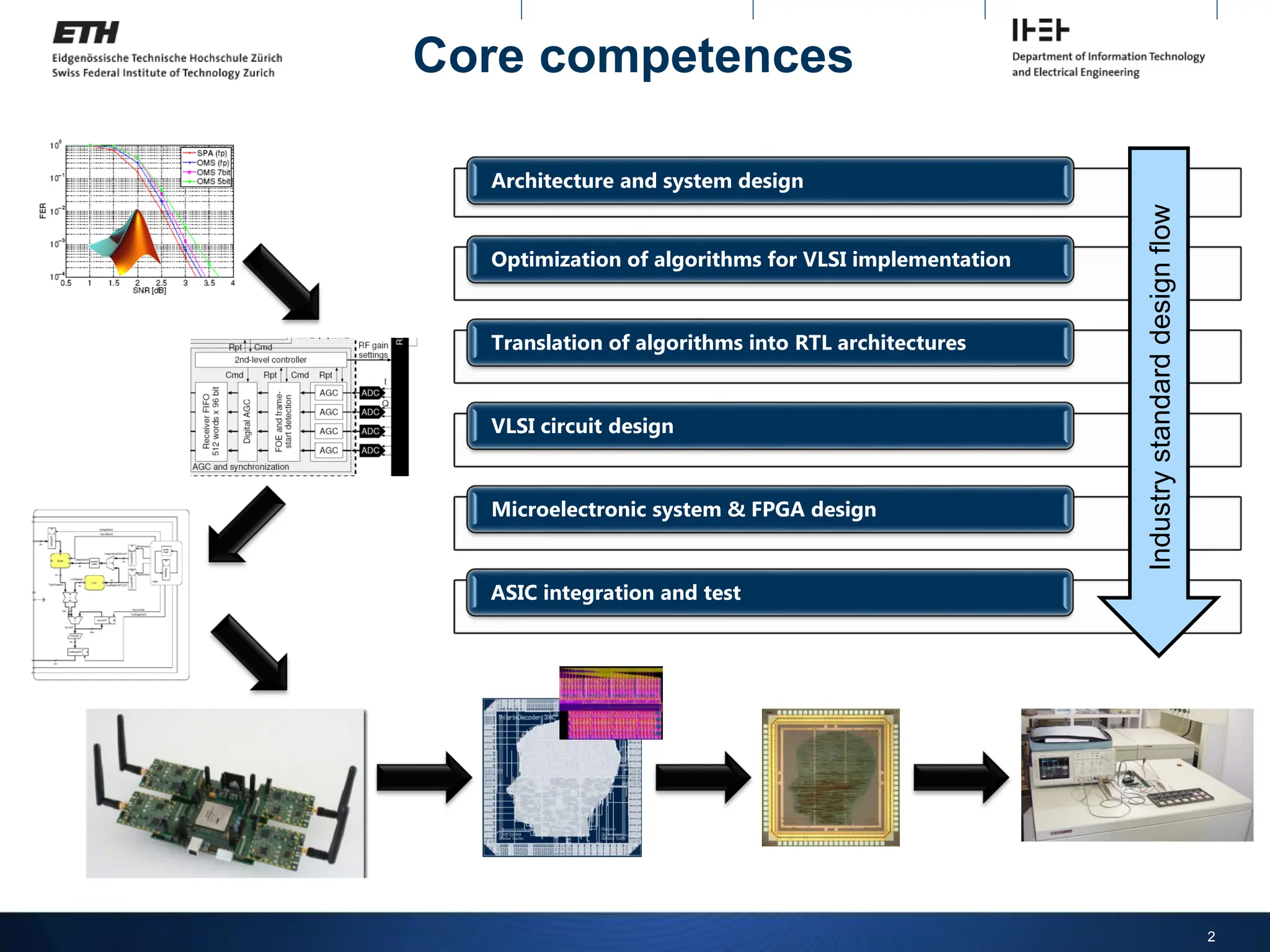
Core competences
Architecture andsystem design
Optimization of algorithms for VLSI implementation
Translation of algorithms into RTL architectures
VLSI circuit design
Microelectronic system & FPGA design
ASIC integration and test
2
Industry
standard
design
flow
3.
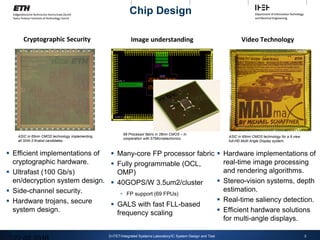
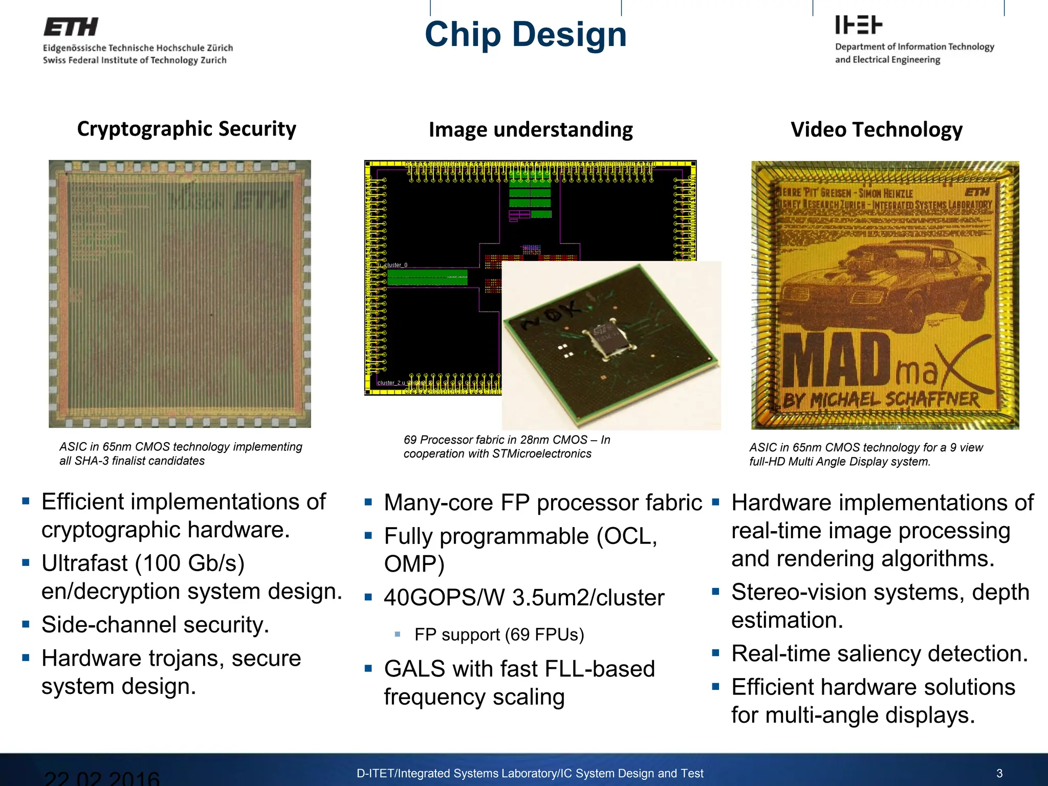
Cryptographic Security
Efficientimplementations of
cryptographic hardware.
Ultrafast (100 Gb/s)
en/decryption system design.
Side-channel security.
Hardware trojans, secure
system design.
3
D-ITET/Integrated Systems Laboratory/IC System Design and Test
ASIC in 65nm CMOS technology implementing
all SHA-3 finalist candidates
Image understanding
Many-core FP processor fabric
Fully programmable (OCL,
OMP)
40GOPS/W 3.5um2/cluster
FP support (69 FPUs)
GALS with fast FLL-based
frequency scaling
69 Processor fabric in 28nm CMOS – In
cooperation with STMicroelectronics
Video Technology
Hardware implementations of
real-time image processing
and rendering algorithms.
Stereo-vision systems, depth
estimation.
Real-time saliency detection.
Efficient hardware solutions
for multi-angle displays.
ASIC in 65nm CMOS technology for a 9 view
full-HD Multi Angle Display system.
Chip Design
5
Departement Informationstechnologie undElektrotechnik
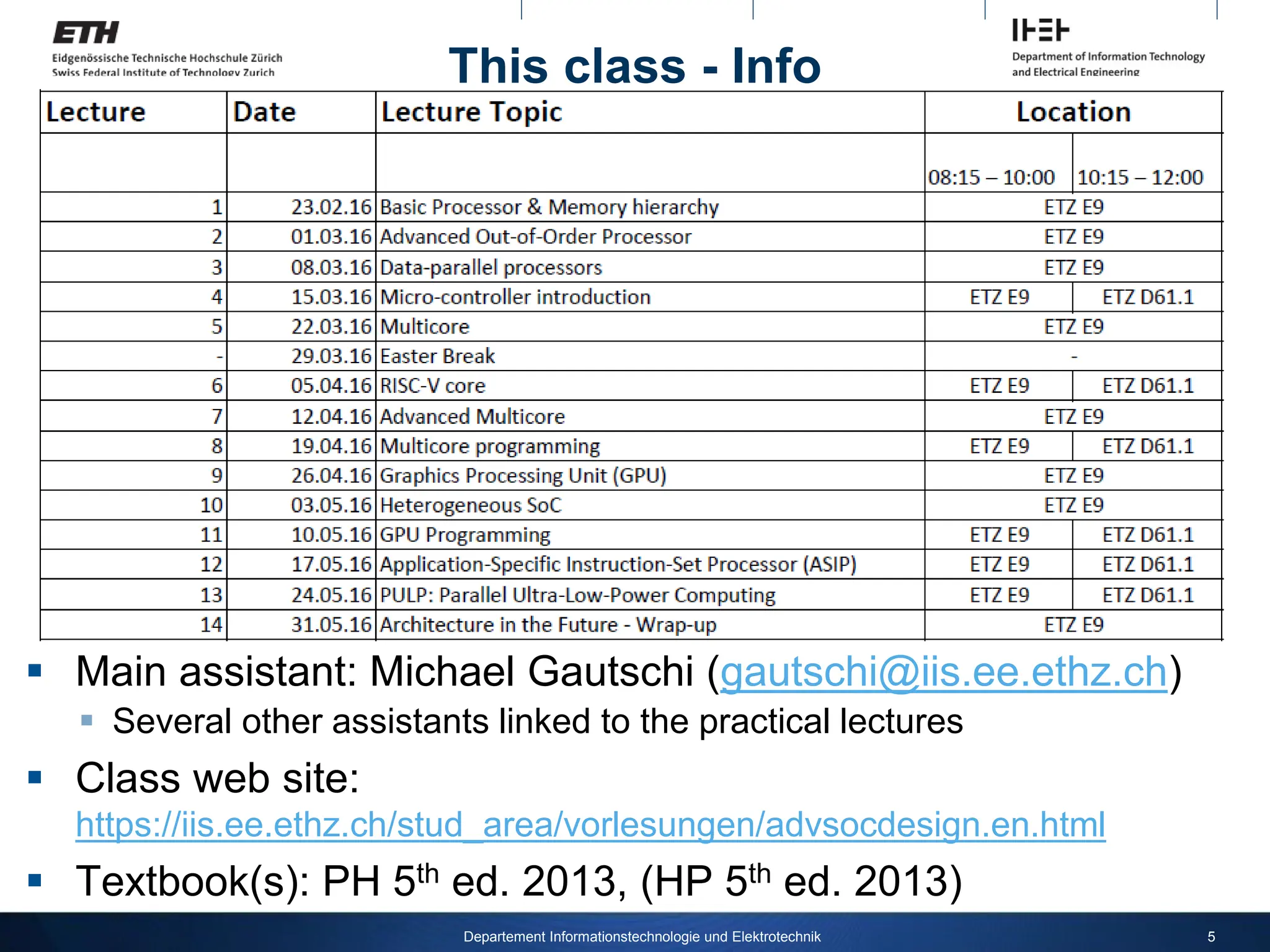
This class - Info
Main assistant: Michael Gautschi (gautschi@iis.ee.ethz.ch)
Several other assistants linked to the practical lectures
Class web site:
https://iis.ee.ethz.ch/stud_area/vorlesungen/advsocdesign.en.html
Textbook(s): PH 5th ed. 2013, (HP 5th ed. 2013)
6.
This Class -Exam
“30 mins. Oral examination in regular period”
Meaning:
2 Questions from lectures – including “pencil and paper” discussion
Discussion on “independent work” – based on a 10min presentation
Directed reading – A set of papers assigned a starting point for a critical
review of the state of the art of a given topic – goal is to understand the
topic and be able to identify areas of exploration
Practical mini-project – Work on one of the topics presented in the
practical exercises – take a mini-project proposed by the assistants, do
the work and present your results
Score is 50% from questions, 50% from discussion
Preparation for the discussion work is either individual or
can done in group of two, but exam is individual
6
Departement Informationstechnologie und Elektrotechnik
7.
COMPUTER ORGANIZATION ANDDESIGN
The Hardware/Software Interface
5th
Edition
Chapter 1
Computer Abstractions
and Technology
8.
Chapter 1 —Computer Abstractions and Technology — 8
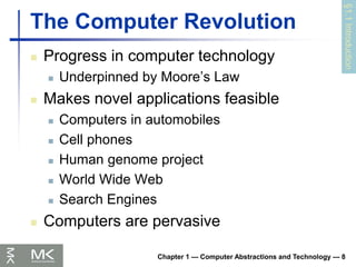
The Computer Revolution
Progress in computer technology
Underpinned by Moore’s Law
Makes novel applications feasible
Computers in automobiles
Cell phones
Human genome project
World Wide Web
Search Engines
Computers are pervasive
§1.1
Introduction
9.
1/18/2012 9
cs252-S12 Lecture-01
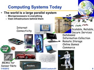
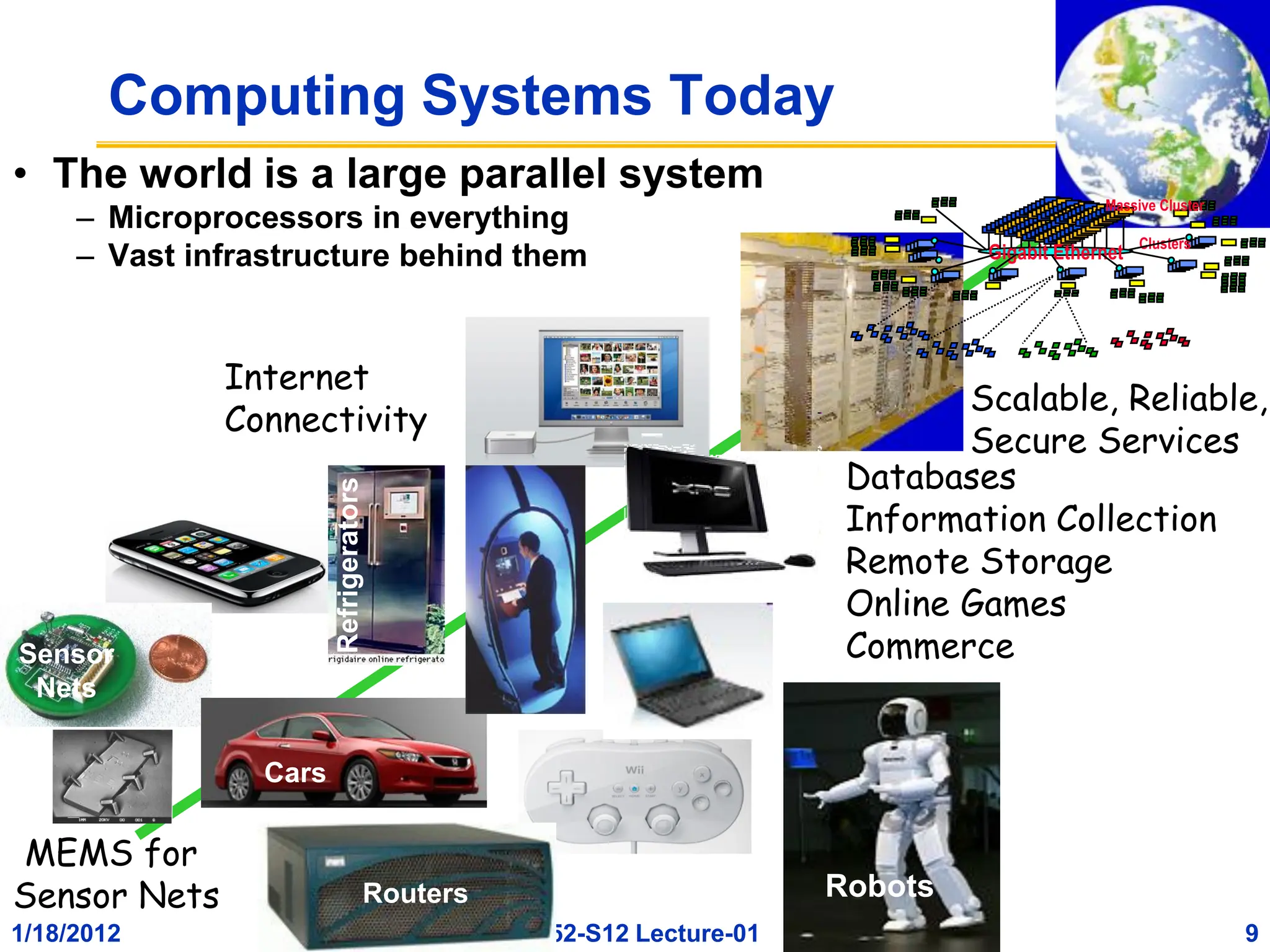
ComputingSystems Today
Scalable, Reliable,
Secure Services
MEMS for
Sensor Nets
Internet
Connectivity
Clusters
Massive Cluster
Gigabit Ethernet
Databases
Information Collection
Remote Storage
Online Games
Commerce
…
• The world is a large parallel system
– Microprocessors in everything
– Vast infrastructure behind them
Robots
Routers
Cars
Sensor
Nets
Refrigerators
10.
Chapter 1 —Computer Abstractions and Technology — 10
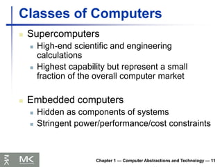
Classes of Computers
Personal computers
General purpose, variety of software
Subject to cost/performance tradeoff
Server computers
Network based
High capacity, performance, reliability
Range from small servers to building sized
11.
Classes of Computers
Supercomputers
High-end scientific and engineering
calculations
Highest capability but represent a small
fraction of the overall computer market
Embedded computers
Hidden as components of systems
Stringent power/performance/cost constraints
Chapter 1 — Computer Abstractions and Technology — 11
12.
Chapter 1 —Computer Abstractions and Technology — 12
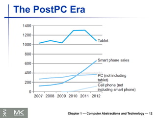
The PostPC Era
13.
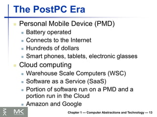
The PostPC Era
Chapter1 — Computer Abstractions and Technology — 13
Personal Mobile Device (PMD)
Battery operated
Connects to the Internet
Hundreds of dollars
Smart phones, tablets, electronic glasses
Cloud computing
Warehouse Scale Computers (WSC)
Software as a Service (SaaS)
Portion of software run on a PMD and a
portion run in the Cloud
Amazon and Google
14.
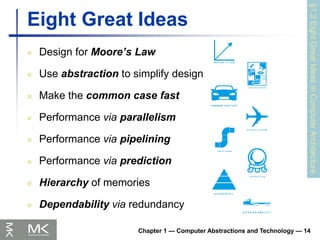
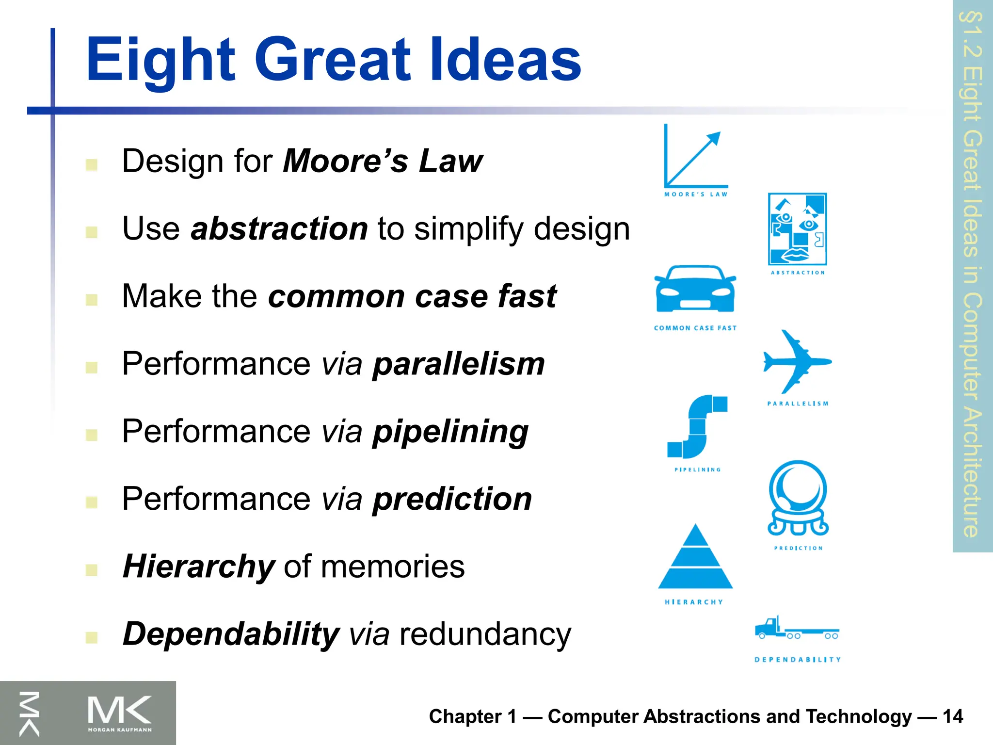
Eight Great Ideas
Design for Moore’s Law
Use abstraction to simplify design
Make the common case fast
Performance via parallelism
Performance via pipelining
Performance via prediction
Hierarchy of memories
Dependability via redundancy
Chapter 1 — Computer Abstractions and Technology — 14
§1.2
Eight
Great
Ideas
in
Computer
Architecture
15.
Chapter 1 —Computer Abstractions and Technology — 15
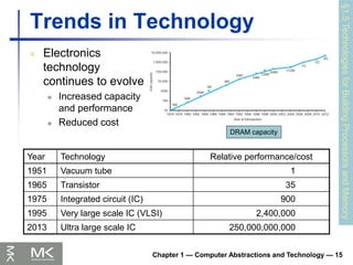
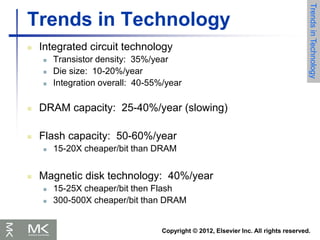
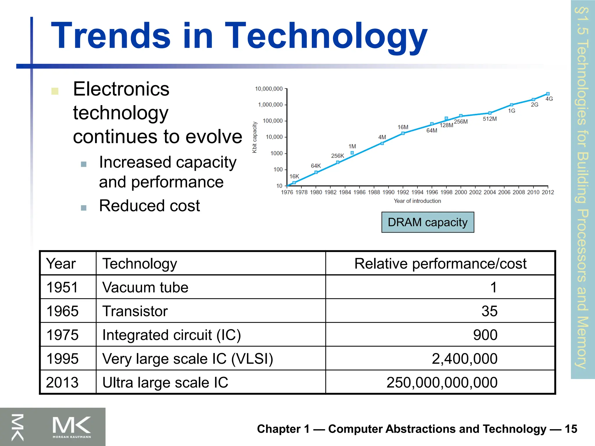
Trends in Technology
Electronics
technology
continues to evolve
Increased capacity
and performance
Reduced cost
Year Technology Relative performance/cost
1951 Vacuum tube 1
1965 Transistor 35
1975 Integrated circuit (IC) 900
1995 Very large scale IC (VLSI) 2,400,000
2013 Ultra large scale IC 250,000,000,000
DRAM capacity
§1.5
Technologies
for
Building
Processors
and
Memory
Chapter 1 —Computer Abstractions and Technology — 18
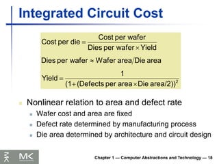
Integrated Circuit Cost
Nonlinear relation to area and defect rate
Wafer cost and area are fixed
Defect rate determined by manufacturing process
Die area determined by architecture and circuit design
2
area/2))
Die
area
per
(Defects
(1
1
Yield
area
Die
area
Wafer
wafer
per
Dies
Yield
wafer
per
Dies
wafer
per
Cost
die
per
Cost
Chapter 1 —Computer Abstractions and Technology — 26
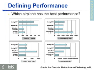
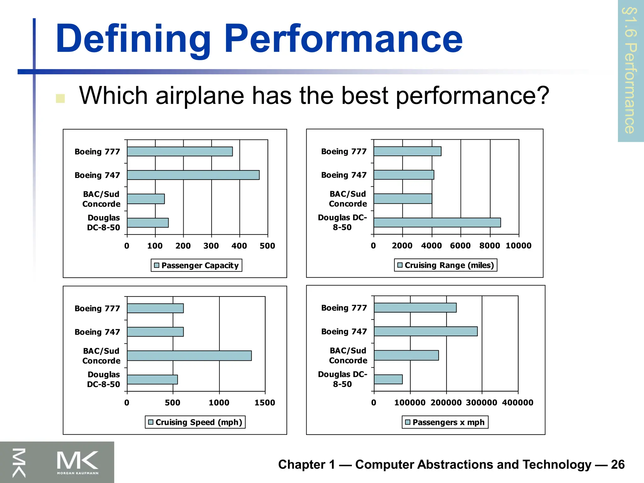
Defining Performance
Which airplane has the best performance?
0 100 200 300 400 500
Douglas
DC-8-50
BAC/Sud
Concorde
Boeing 747
Boeing 777
Passenger Capacity
0 2000 4000 6000 8000 10000
Douglas DC-
8-50
BAC/Sud
Concorde
Boeing 747
Boeing 777
Cruising Range (miles)
0 500 1000 1500
Douglas
DC-8-50
BAC/Sud
Concorde
Boeing 747
Boeing 777
Cruising Speed (mph)
0 100000 200000 300000 400000
Douglas DC-
8-50
BAC/Sud
Concorde
Boeing 747
Boeing 777
Passengers x mph
§1.6
Performance
27.
Chapter 1 —Computer Abstractions and Technology — 27
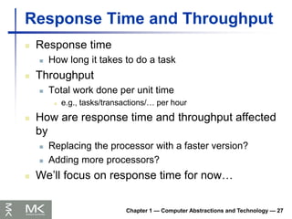
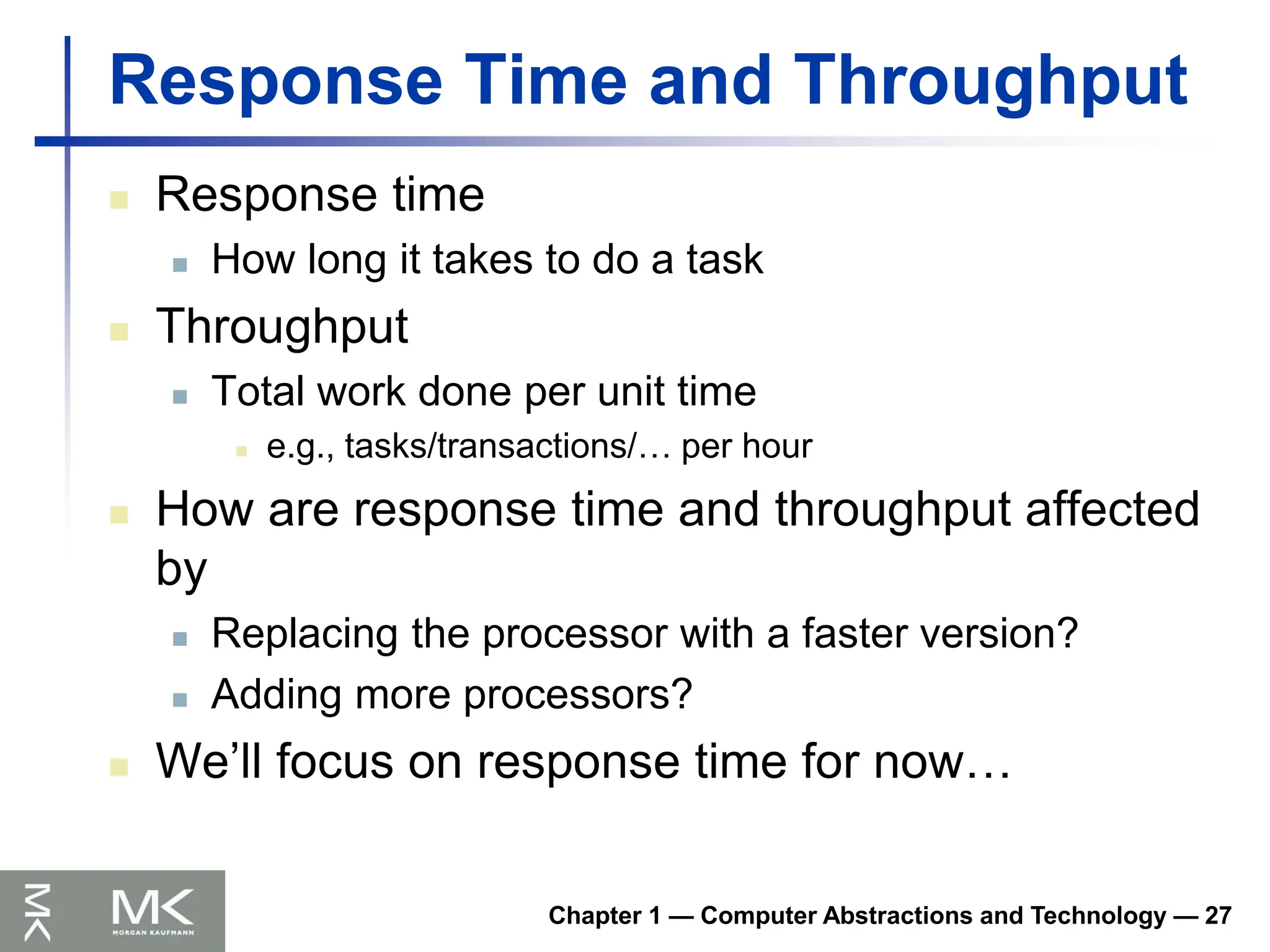
Response Time and Throughput
Response time
How long it takes to do a task
Throughput
Total work done per unit time
e.g., tasks/transactions/… per hour
How are response time and throughput affected
by
Replacing the processor with a faster version?
Adding more processors?
We’ll focus on response time for now…
28.
Chapter 1 —Computer Abstractions and Technology — 28
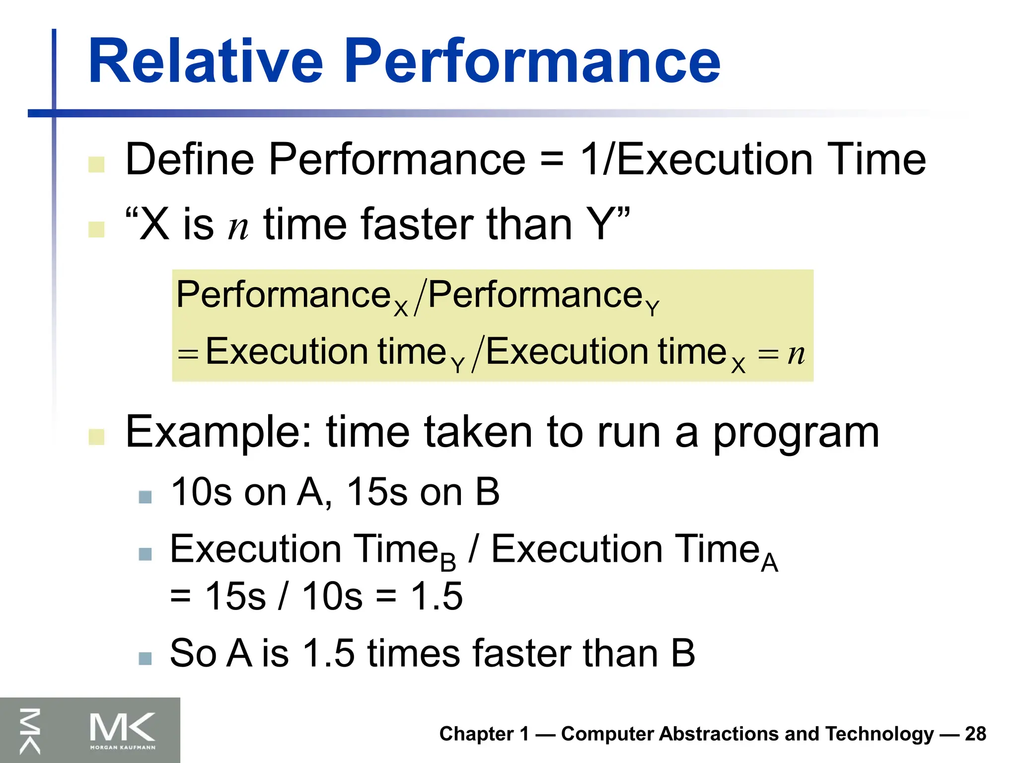
Relative Performance
Define Performance = 1/Execution Time
“X is n time faster than Y”
n
X
Y
Y
X
time
Execution
time
Execution
e
Performanc
e
Performanc
Example: time taken to run a program
10s on A, 15s on B
Execution TimeB / Execution TimeA
= 15s / 10s = 1.5
So A is 1.5 times faster than B
29.
Chapter 1 —Computer Abstractions and Technology — 29
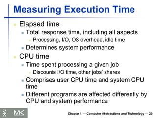
Measuring Execution Time
Elapsed time
Total response time, including all aspects
Processing, I/O, OS overhead, idle time
Determines system performance
CPU time
Time spent processing a given job
Discounts I/O time, other jobs’ shares
Comprises user CPU time and system CPU
time
Different programs are affected differently by
CPU and system performance
30.
Chapter 1 —Computer Abstractions and Technology — 30
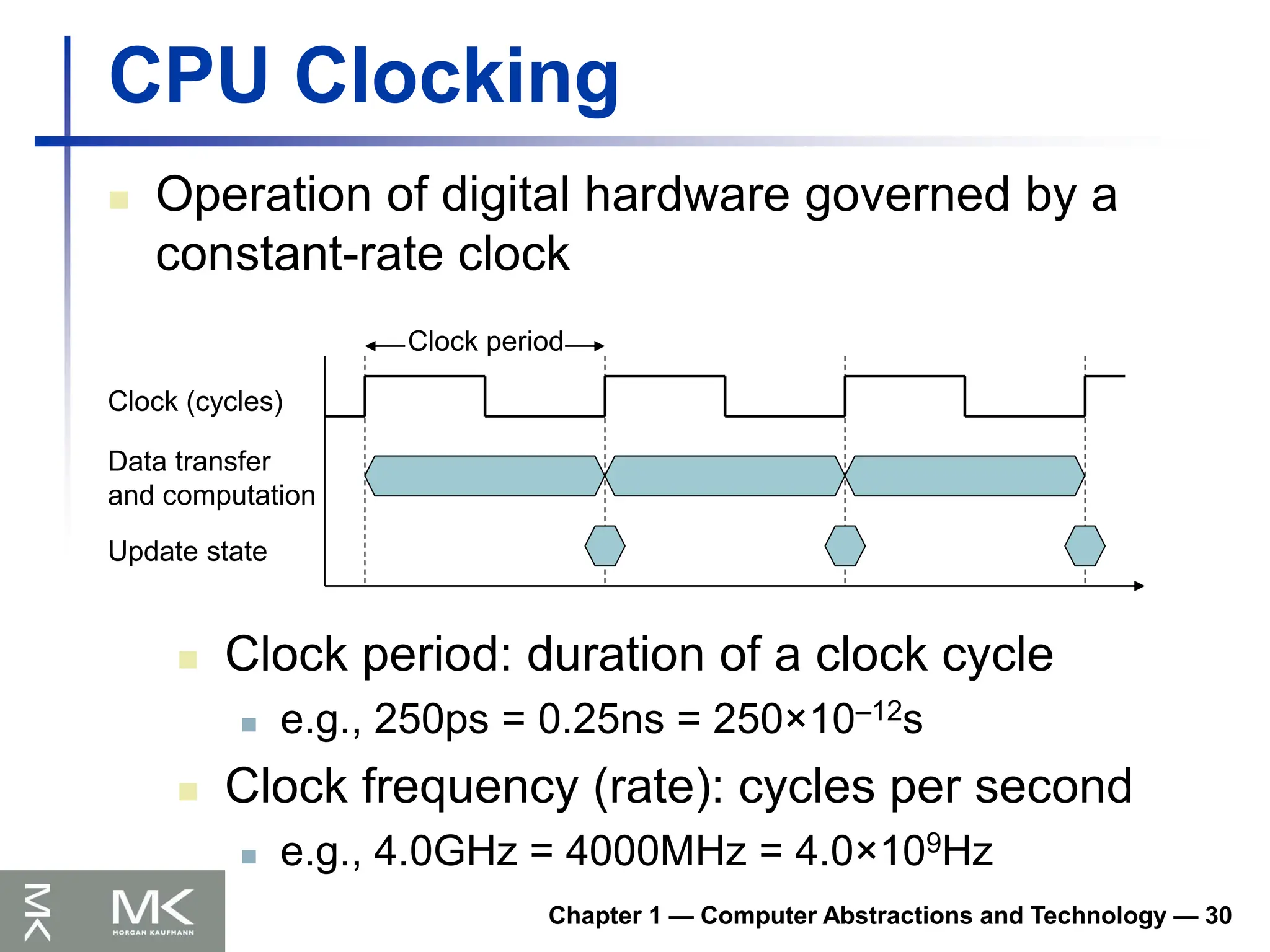
CPU Clocking
Operation of digital hardware governed by a
constant-rate clock
Clock (cycles)
Data transfer
and computation
Update state
Clock period
Clock period: duration of a clock cycle
e.g., 250ps = 0.25ns = 250×10–12s
Clock frequency (rate): cycles per second
e.g., 4.0GHz = 4000MHz = 4.0×10⁹Hz
31.
Chapter 1 —Computer Abstractions and Technology — 31
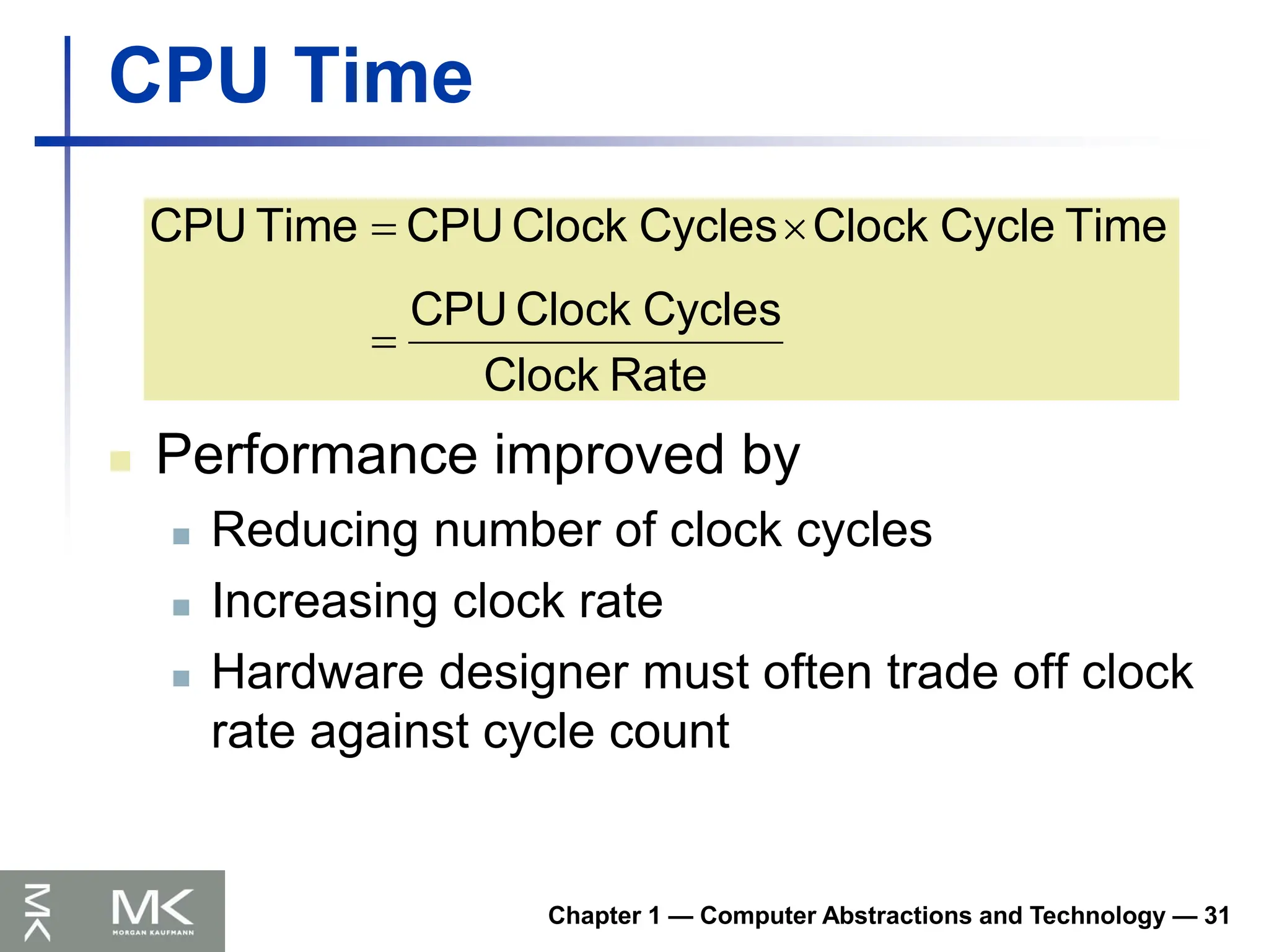
CPU Time
Performance improved by
Reducing number of clock cycles
Increasing clock rate
Hardware designer must often trade off clock
rate against cycle count
Rate
Clock
Cycles
Clock
CPU
Time
Cycle
Clock
Cycles
Clock
CPU
Time
CPU
32.
Chapter 1 —Computer Abstractions and Technology — 32
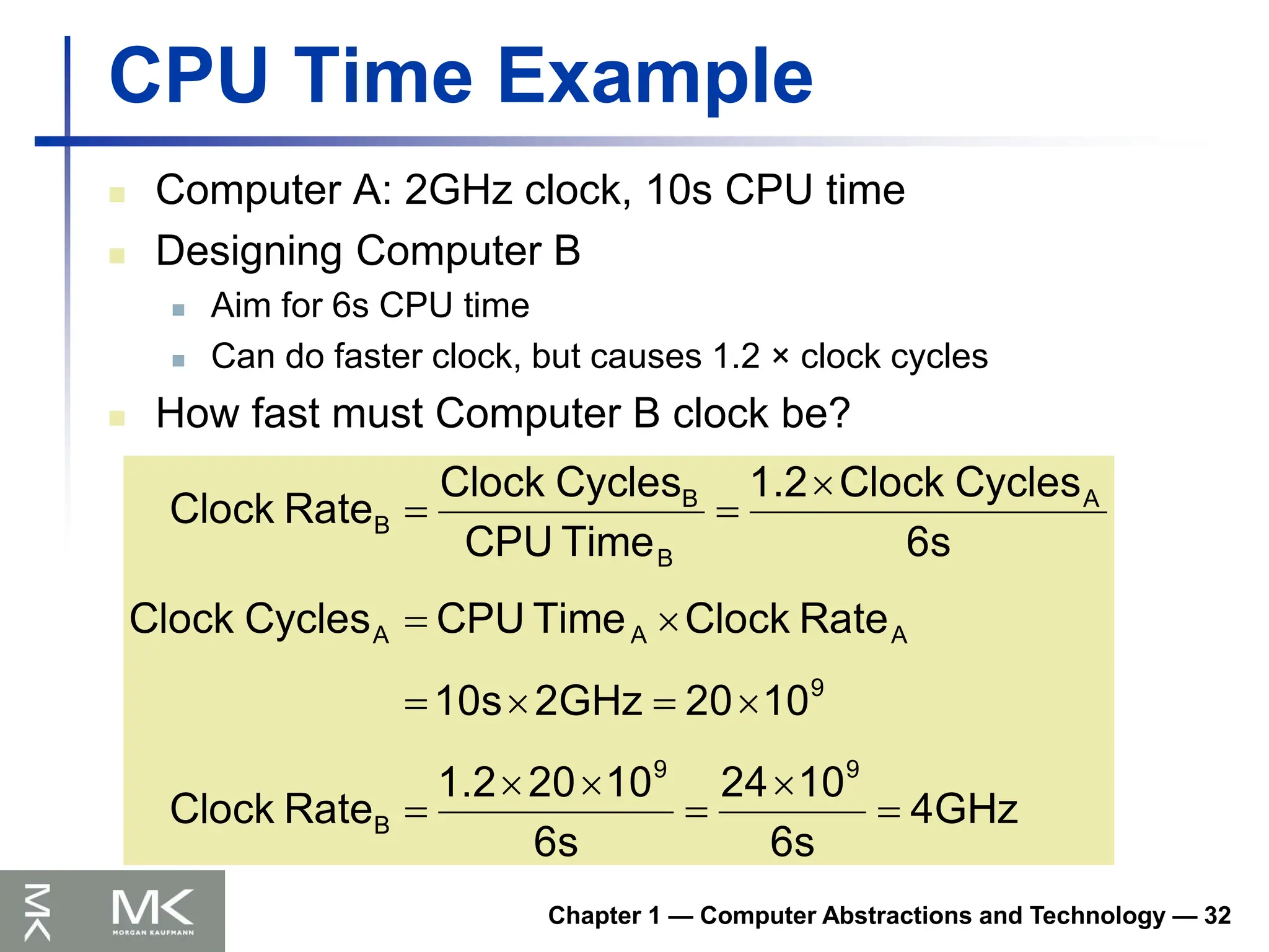
CPU Time Example
Computer A: 2GHz clock, 10s CPU time
Designing Computer B
Aim for 6s CPU time
Can do faster clock, but causes 1.2 × clock cycles
How fast must Computer B clock be?
4GHz
6s
10
24
6s
10
20
1.2
Rate
Clock
10
20
2GHz
10s
Rate
Clock
Time
CPU
Cycles
Clock
6s
Cycles
Clock
1.2
Time
CPU
Cycles
Clock
Rate
Clock
9
9
B
9
A
A
A
A
B
B
B
33.
Chapter 1 —Computer Abstractions and Technology — 33
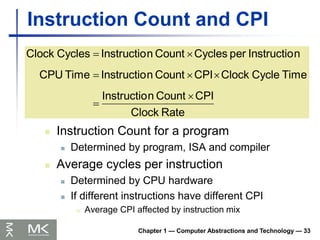
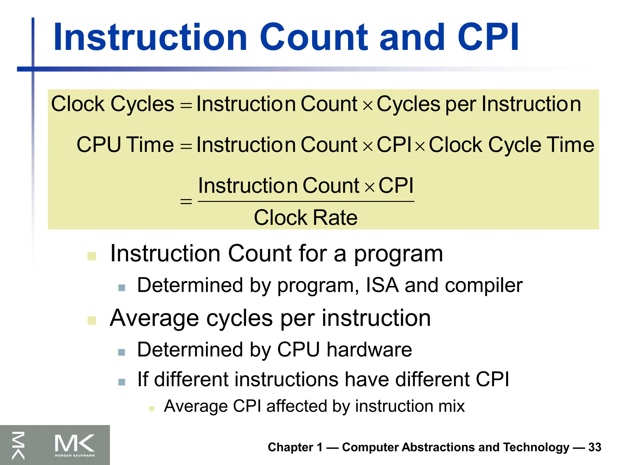
Instruction Count and CPI
Instruction Count for a program
Determined by program, ISA and compiler
Average cycles per instruction
Determined by CPU hardware
If different instructions have different CPI
Average CPI affected by instruction mix
Rate
Clock
CPI
Count
n
Instructio
Time
Cycle
Clock
CPI
Count
n
Instructio
Time
CPU
n
Instructio
per
Cycles
Count
n
Instructio
Cycles
Clock
34.
Chapter 1 —Computer Abstractions and Technology — 34
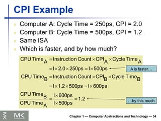
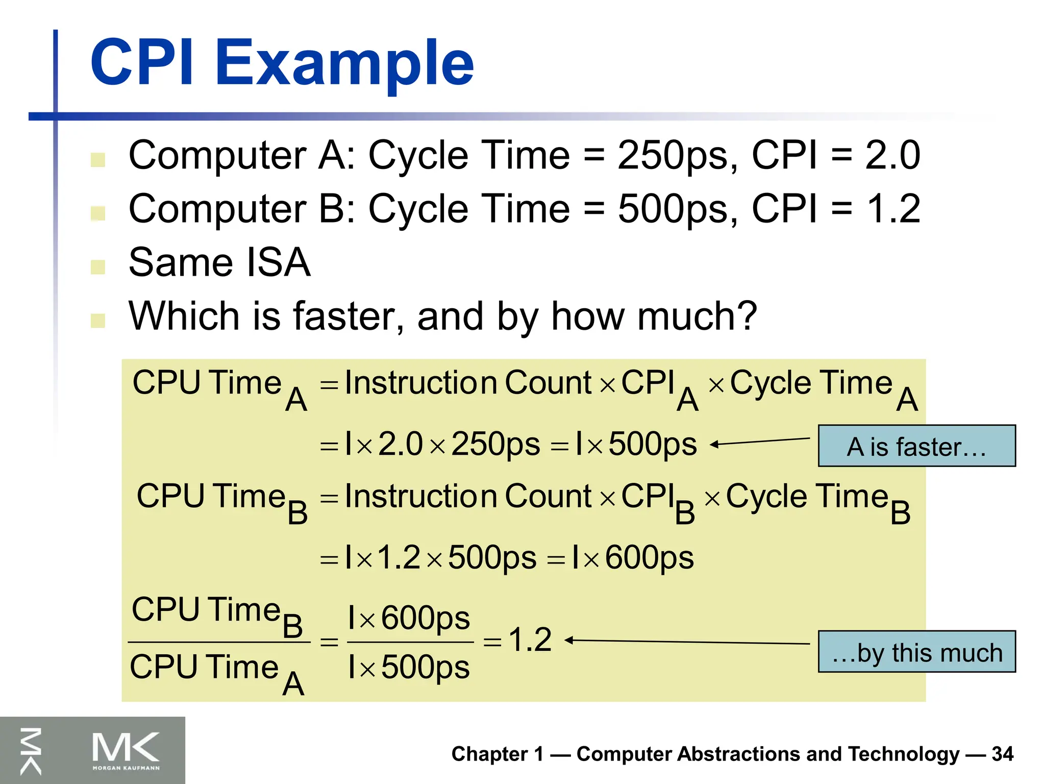
CPI Example
Computer A: Cycle Time = 250ps, CPI = 2.0
Computer B: Cycle Time = 500ps, CPI = 1.2
Same ISA
Which is faster, and by how much?
1.2
500ps
I
600ps
I
A
Time
CPU
B
Time
CPU
600ps
I
500ps
1.2
I
B
Time
Cycle
B
CPI
Count
n
Instructio
B
Time
CPU
500ps
I
250ps
2.0
I
A
Time
Cycle
A
CPI
Count
n
Instructio
A
Time
CPU
A is faster…
…by this much
35.
Chapter 1 —Computer Abstractions and Technology — 35
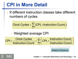
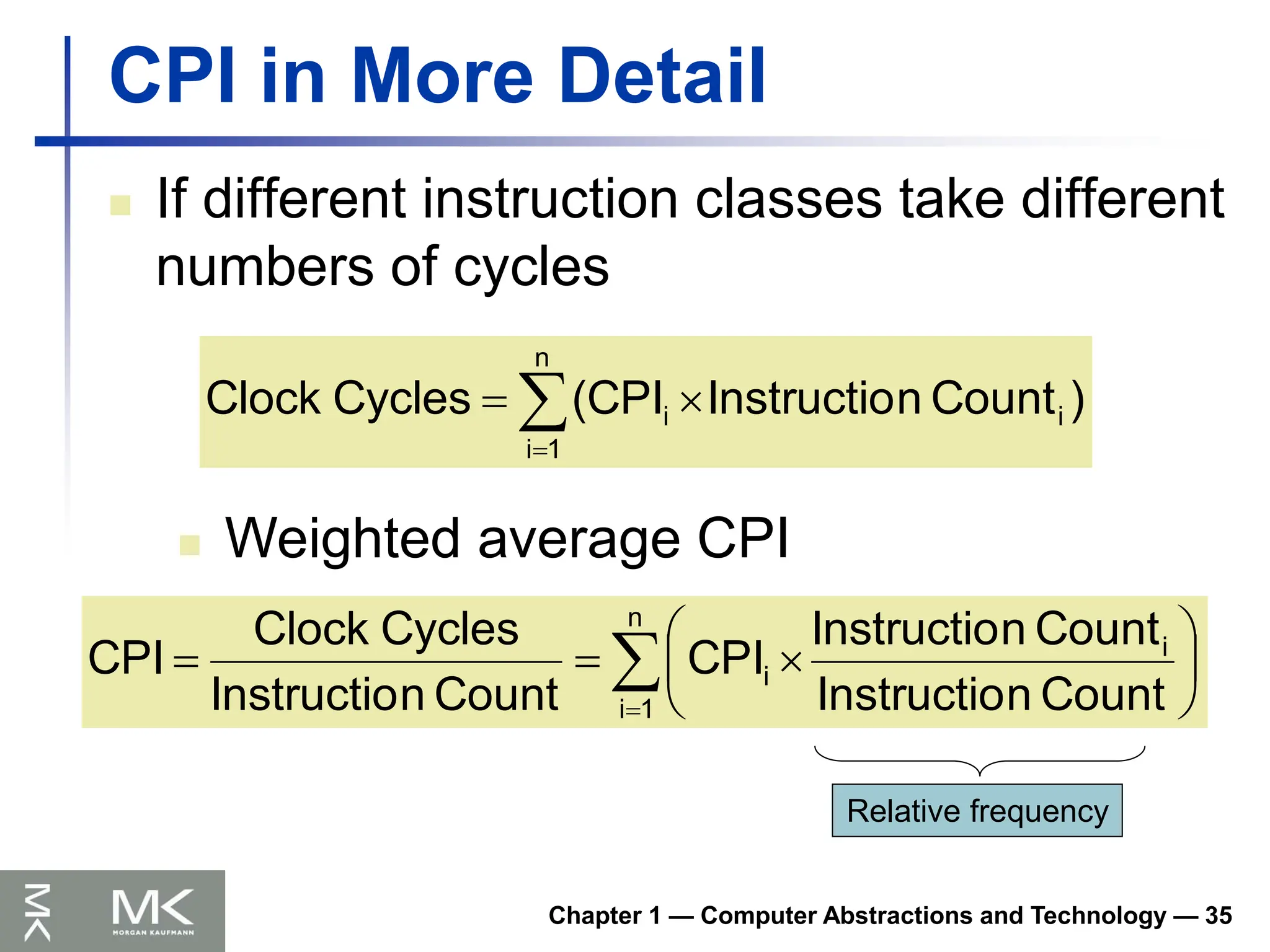
CPI in More Detail
If different instruction classes take different
numbers of cycles
n
1
i
i
i )
Count
n
Instructio
(CPI
Cycles
Clock
Weighted average CPI
n
1
i
i
i
Count
n
Instructio
Count
n
Instructio
CPI
Count
n
Instructio
Cycles
Clock
CPI
Relative frequency
36.
Chapter 1 —Computer Abstractions and Technology — 36
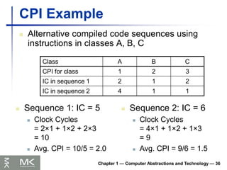
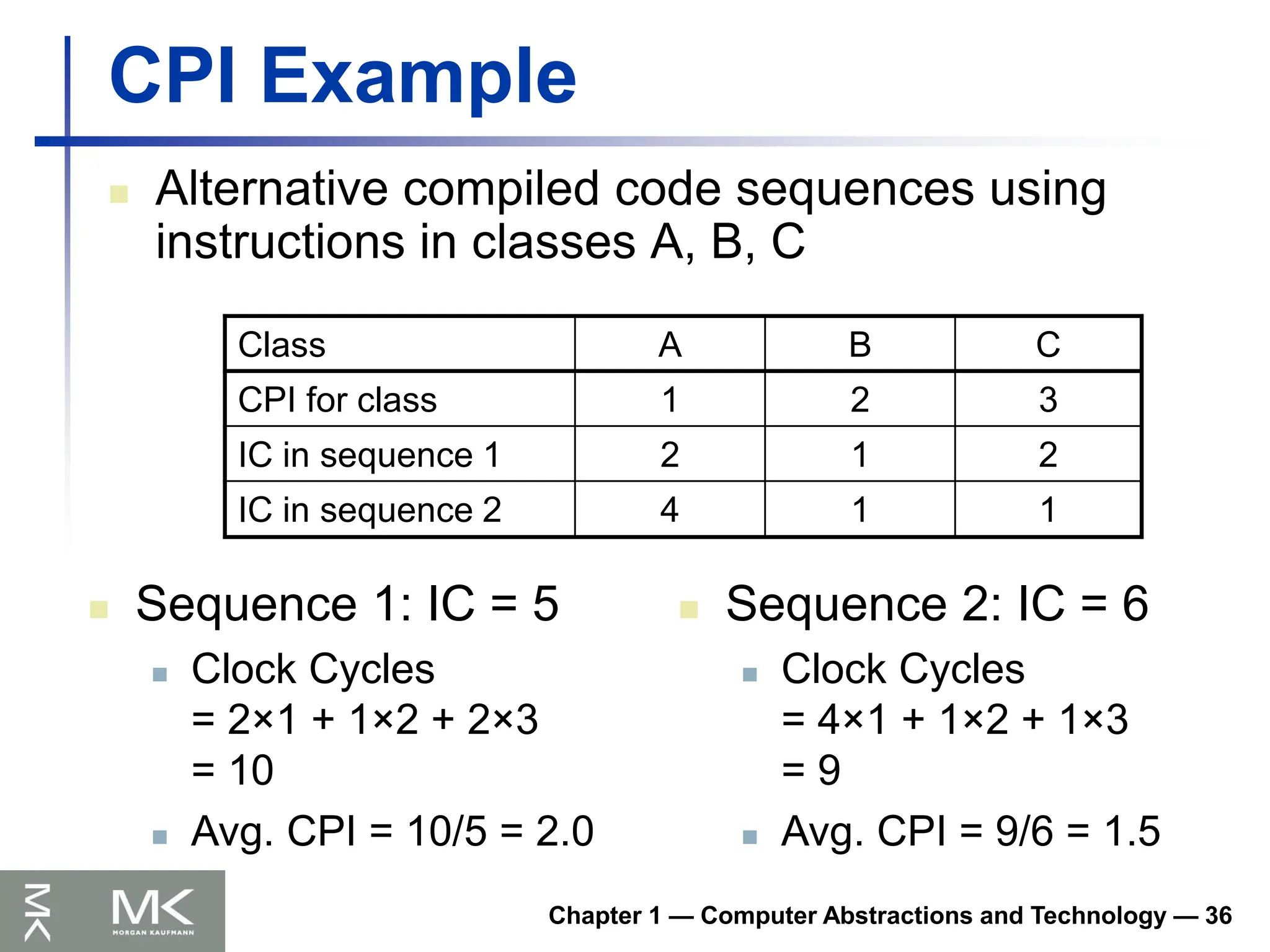
CPI Example
Alternative compiled code sequences using
instructions in classes A, B, C
Class A B C
CPI for class 1 2 3
IC in sequence 1 2 1 2
IC in sequence 2 4 1 1
Sequence 1: IC = 5
Clock Cycles
= 2×1 + 1×2 + 2×3
= 10
Avg. CPI = 10/5 = 2.0
Sequence 2: IC = 6
Clock Cycles
= 4×1 + 1×2 + 1×3
= 9
Avg. CPI = 9/6 = 1.5
37.
Chapter 1 —Computer Abstractions and Technology — 37
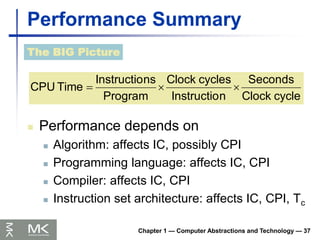
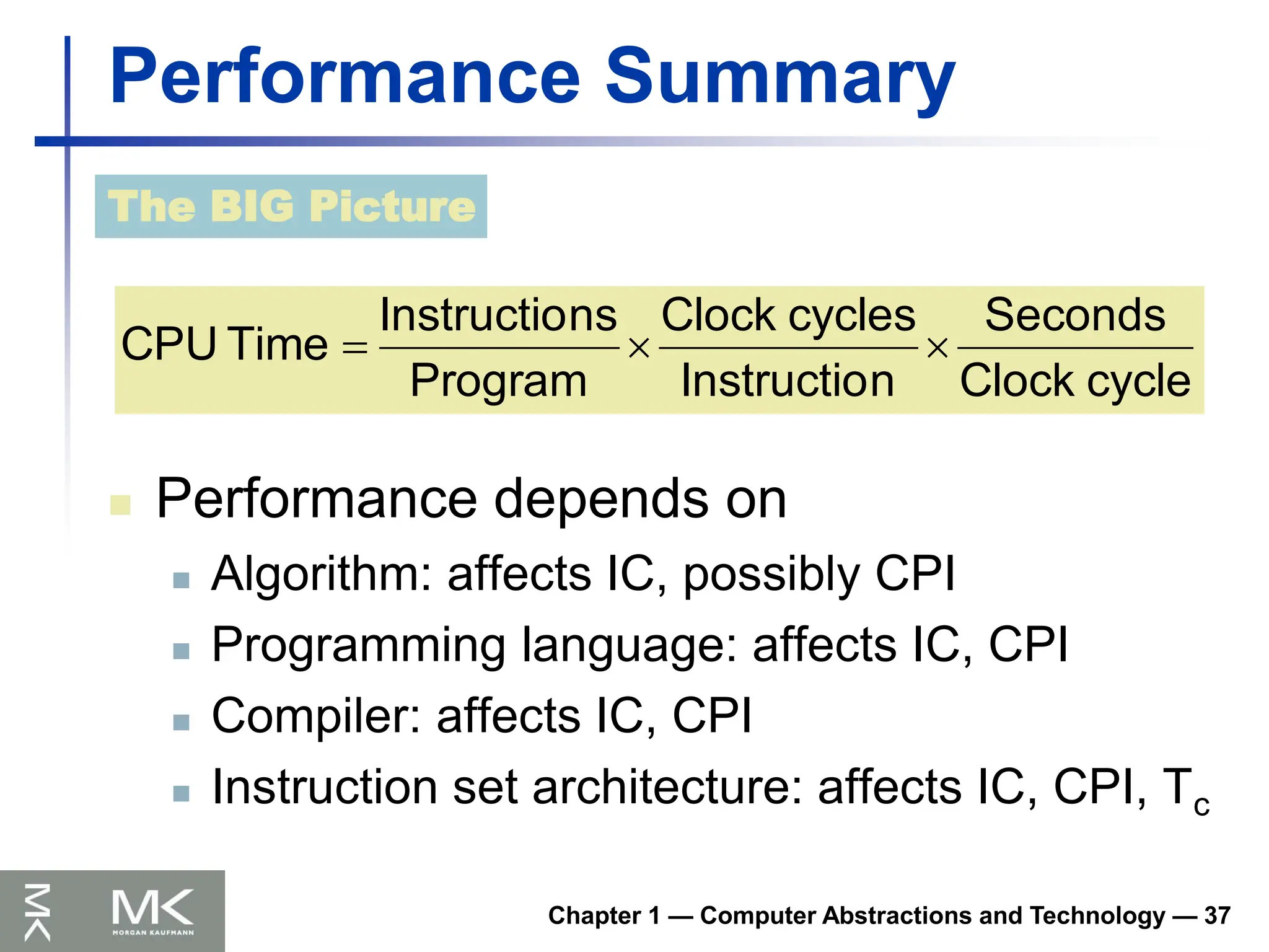
Performance Summary
Performance depends on
Algorithm: affects IC, possibly CPI
Programming language: affects IC, CPI
Compiler: affects IC, CPI
Instruction set architecture: affects IC, CPI, Tc
The BIG Picture
cycle
Clock
Seconds
n
Instructio
cycles
Clock
Program
ns
Instructio
Time
CPU
38.
Chapter 1 —Computer Abstractions and Technology — 38
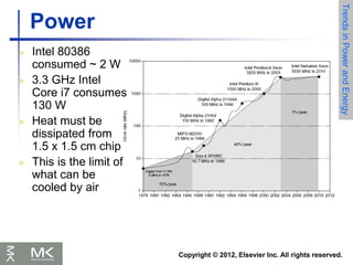
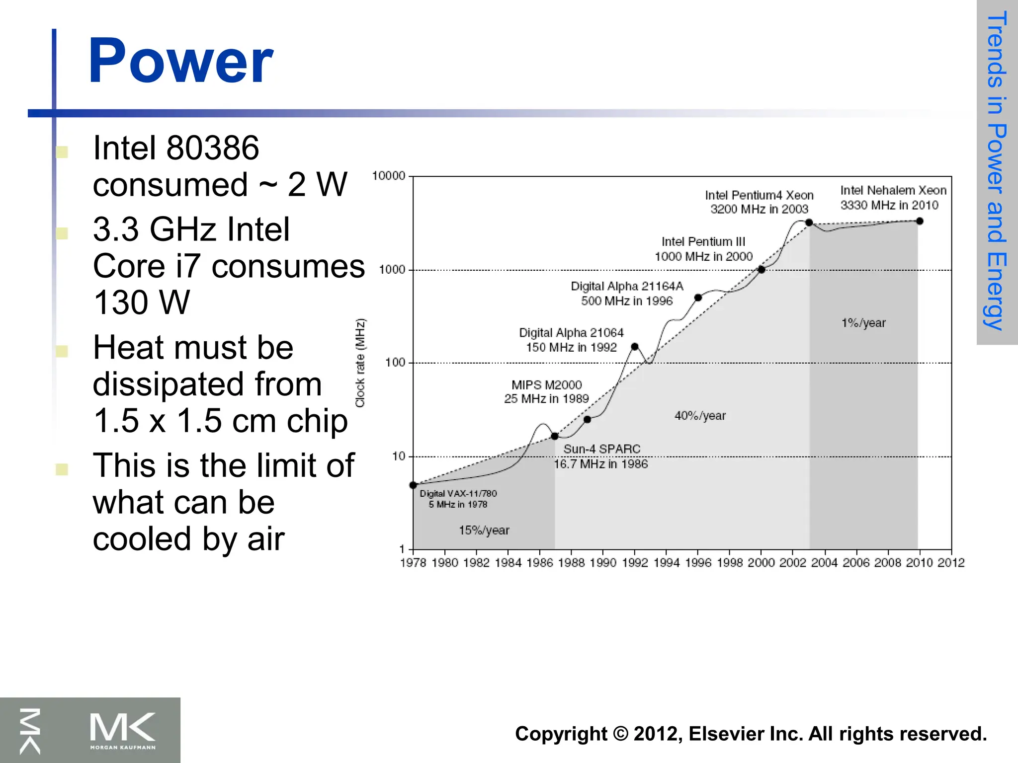
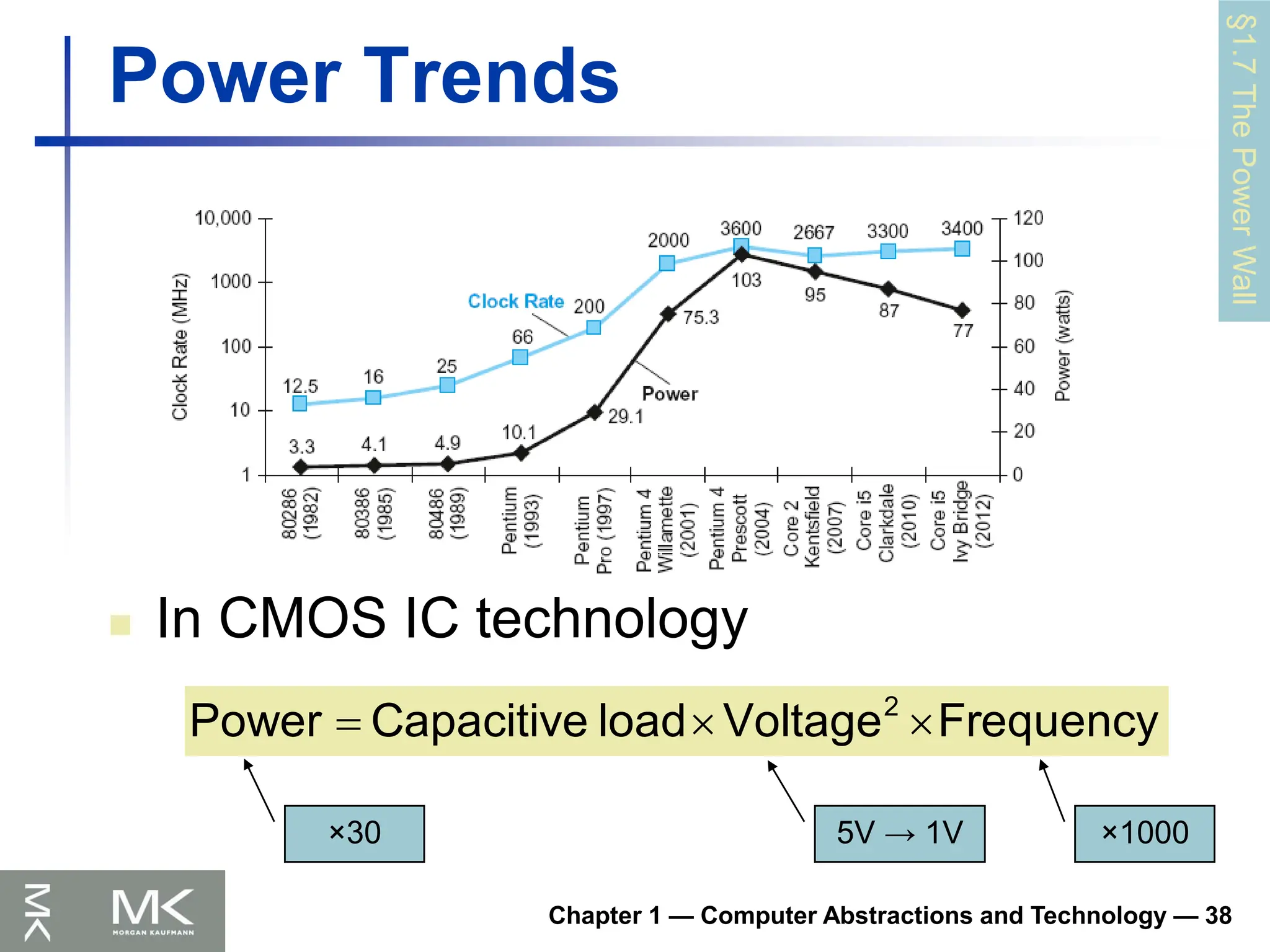
Power Trends
In CMOS IC technology
§1.7
The
Power
Wall
Frequency
Voltage
load
Capacitive
Power 2
×1000
×30 5V → 1V
39.
Chapter 1 —Computer Abstractions and Technology — 39
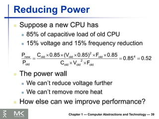
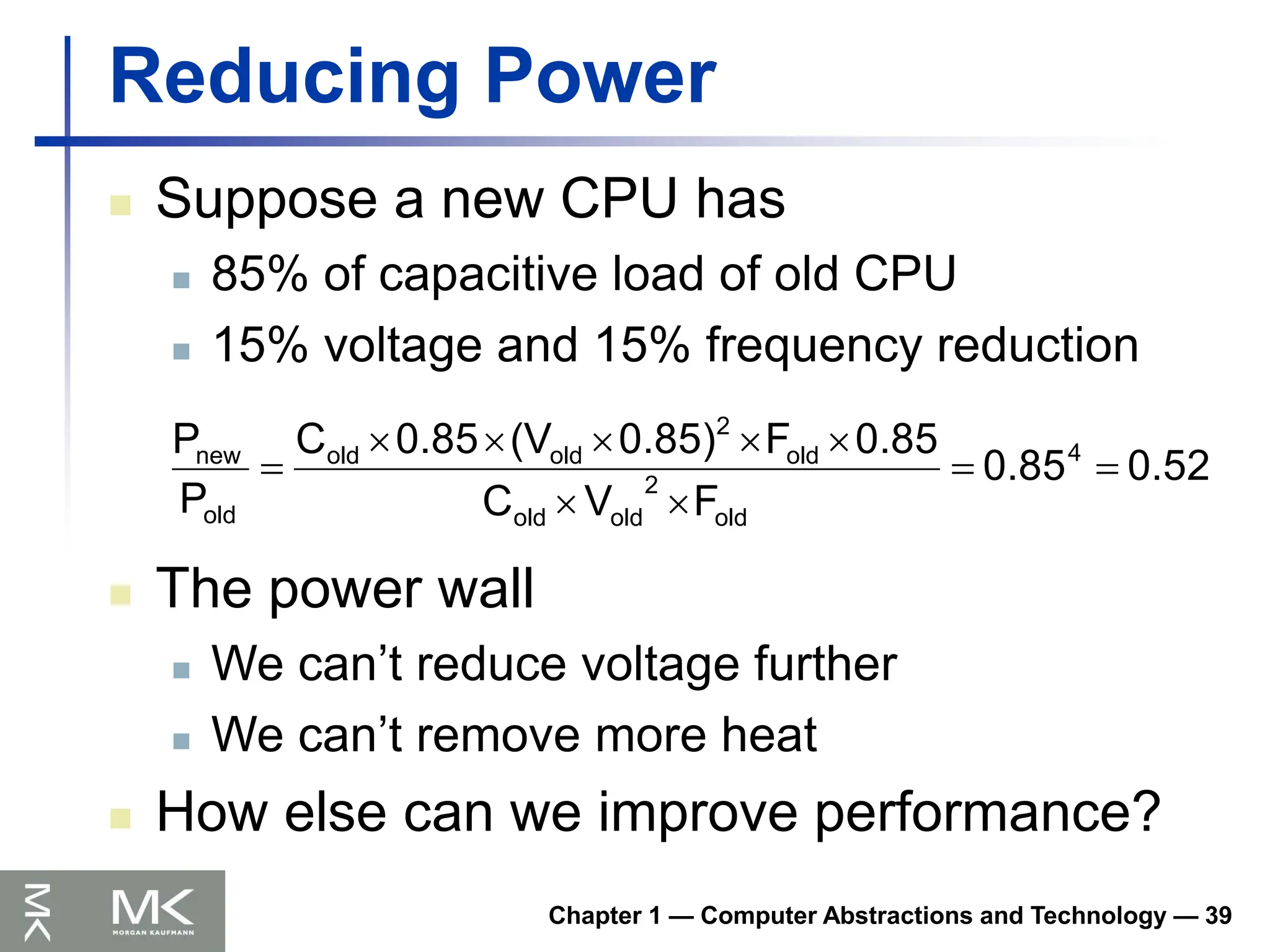
Reducing Power
Suppose a new CPU has
85% of capacitive load of old CPU
15% voltage and 15% frequency reduction
0.52
0.85
F
V
C
0.85
F
0.85)
(V
0.85
C
P
P 4
old
2
old
old
old
2
old
old
old
new
The power wall
We can’t reduce voltage further
We can’t remove more heat
How else can we improve performance?
40.
Chapter 1 —Computer Abstractions and Technology — 40
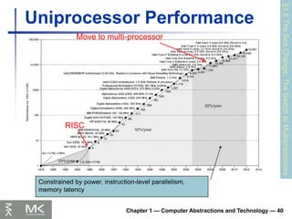
Uniprocessor Performance
§1.8
The
Sea
Change:
The
Switch
to
Multiprocessors
Constrained by power, instruction-level parallelism,
memory latency
RISC
Move to multi-processor
41.
Chapter 1 —Computer Abstractions and Technology — 41
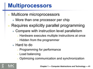
Multiprocessors
Multicore microprocessors
More than one processor per chip
Requires explicitly parallel programming
Compare with instruction level parallelism
Hardware executes multiple instructions at once
Hidden from the programmer
Hard to do
Programming for performance
Load balancing
Optimizing communication and synchronization
42.
Chapter 1 —Computer Abstractions and Technology — 42
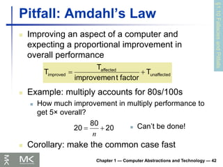
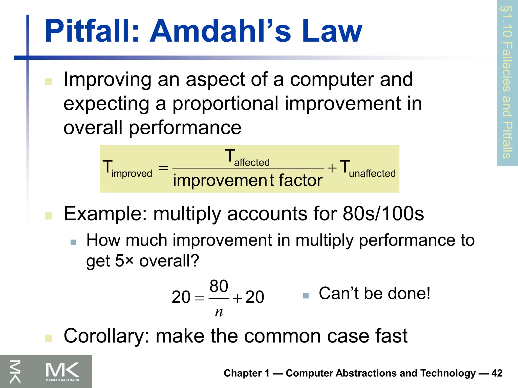
Pitfall: Amdahl’s Law
Improving an aspect of a computer and
expecting a proportional improvement in
overall performance
§1.10
Fallacies
and
Pitfalls
20
80
20
n
Can’t be done!
unaffected
affected
improved T
factor
t
improvemen
T
T
Example: multiply accounts for 80s/100s
How much improvement in multiply performance to
get 5× overall?
Corollary: make the common case fast
43.
Chapter 1 —Computer Abstractions and Technology — 43
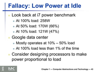
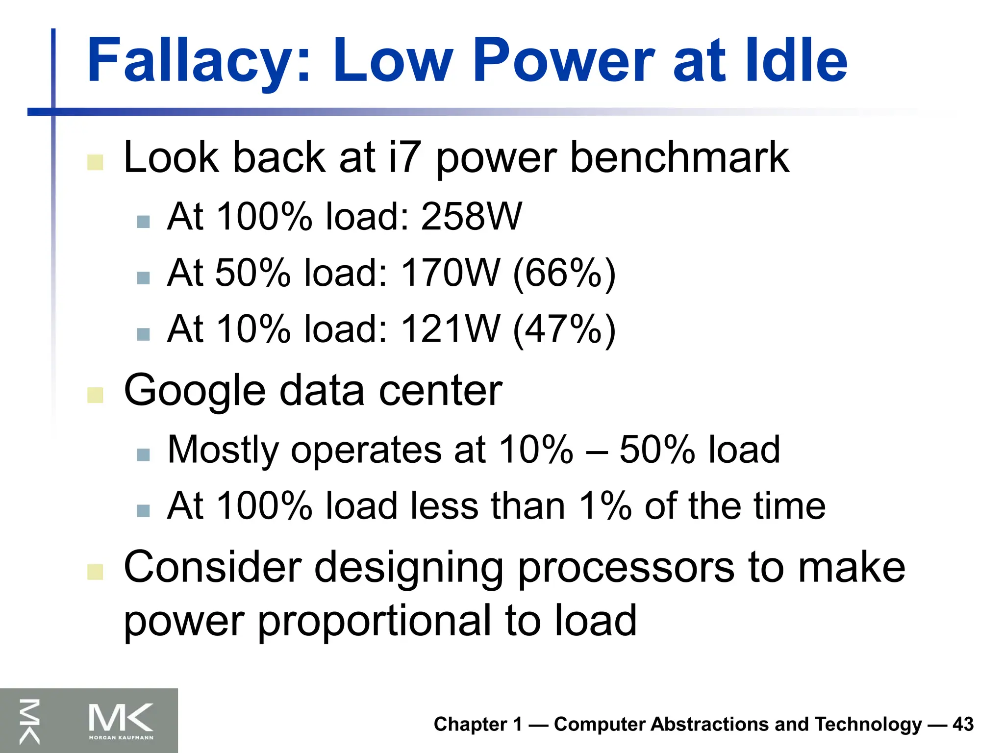
Fallacy: Low Power at Idle
Look back at i7 power benchmark
At 100% load: 258W
At 50% load: 170W (66%)
At 10% load: 121W (47%)
Google data center
Mostly operates at 10% – 50% load
At 100% load less than 1% of the time
Consider designing processors to make
power proportional to load
44.
Chapter 1 —Computer Abstractions and Technology — 44
Concluding Remarks
Cost/performance is improving
Due to underlying technology development
Hierarchical layers of abstraction
In both hardware and software
Instruction set architecture
The hardware/software interface
Execution time: the best performance
measure
Power is a limiting factor
Use parallelism to improve performance
§1.9
Concluding
Remarks
45.
COMPUTER ORGANIZATION ANDDESIGN
The Hardware/Software Interface
5th
Edition
Chapter 2
Instructions: Language
of the Computer
46.
Chapter 2 —Instructions: Language of the Computer — 2
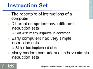
Instruction Set
The repertoire of instructions of a
computer
Different computers have different
instruction sets
But with many aspects in common
Early computers had very simple
instruction sets
Simplified implementation
Many modern computers also have simple
instruction sets
§2.1
Introduction
47.
Chapter 2 —Instructions: Language of the Computer — 3
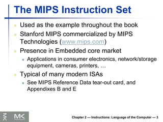
The MIPS Instruction Set
Used as the example throughout the book
Stanford MIPS commercialized by MIPS
Technologies (www.mips.com)
Presence in Embedded core market
Applications in consumer electronics, network/storage
equipment, cameras, printers, …
Typical of many modern ISAs
See MIPS Reference Data tear-out card, and
Appendixes B and E
48.
Chapter 2 —Instructions: Language of the Computer — 4
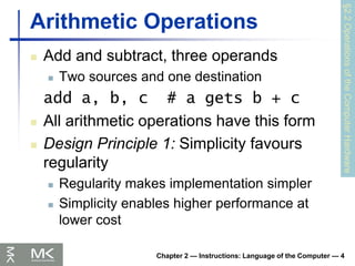
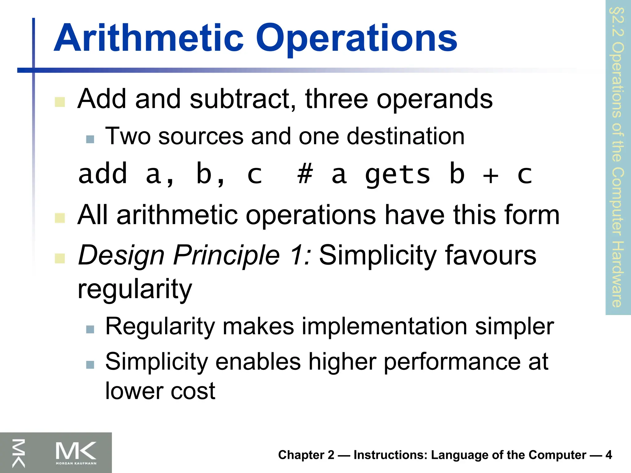
Arithmetic Operations
Add and subtract, three operands
Two sources and one destination
add a, b, c # a gets b + c
All arithmetic operations have this form
Design Principle 1: Simplicity favours
regularity
Regularity makes implementation simpler
Simplicity enables higher performance at
lower cost
§2.2
Operations
of
the
Computer
Hardware
49.
Chapter 2 —Instructions: Language of the Computer — 5
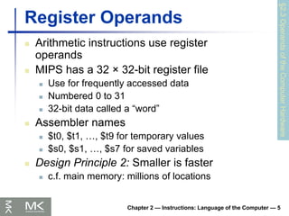
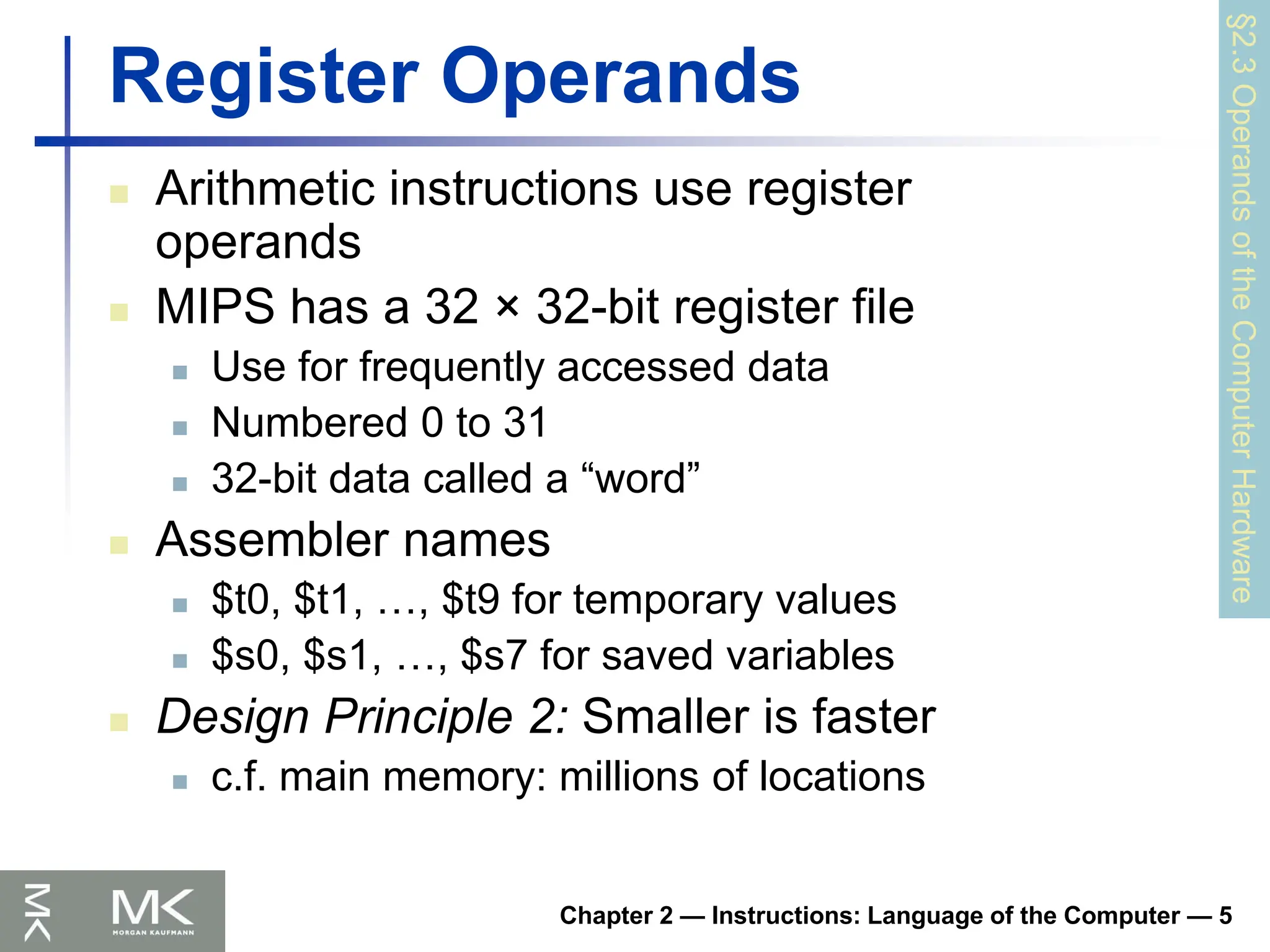
Register Operands
Arithmetic instructions use register
operands
MIPS has a 32 × 32-bit register file
Use for frequently accessed data
Numbered 0 to 31
32-bit data called a “word”
Assembler names
$t0, $t1, …, $t9 for temporary values
$s0, $s1, …, $s7 for saved variables
Design Principle 2: Smaller is faster
c.f. main memory: millions of locations
§2.3
Operands
of
the
Computer
Hardware
50.
Chapter 2 —Instructions: Language of the Computer — 6
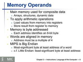
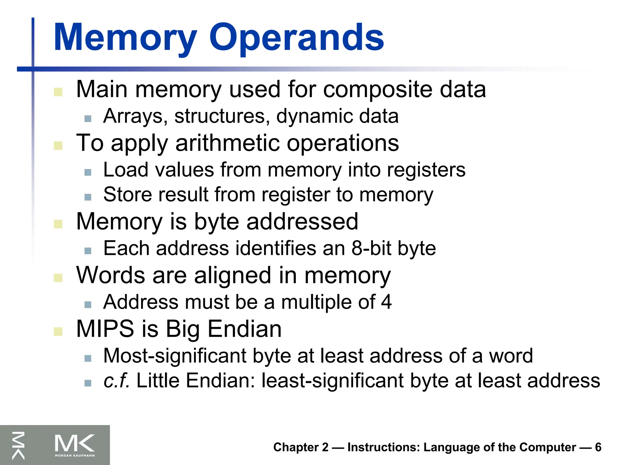
Memory Operands
Main memory used for composite data
Arrays, structures, dynamic data
To apply arithmetic operations
Load values from memory into registers
Store result from register to memory
Memory is byte addressed
Each address identifies an 8-bit byte
Words are aligned in memory
Address must be a multiple of 4
MIPS is Big Endian
Most-significant byte at least address of a word
c.f. Little Endian: least-significant byte at least address
51.
Chapter 2 —Instructions: Language of the Computer — 7
Memory Operand Example 1
C code:
g = h + A[8];
g in $s1, h in $s2, base address of A in $s3
Compiled MIPS code:
Index 8 requires offset of 32
4 bytes per word
lw $t0, 32($s3) # load word
add $s1, $s2, $t0
offset base register
52.
Chapter 2 —Instructions: Language of the Computer — 8
Memory Operand Example 2
C code:
A[12] = h + A[8];
h in $s2, base address of A in $s3
Compiled MIPS code:
Index 8 requires offset of 32
lw $t0, 32($s3) # load word
add $t0, $s2, $t0
sw $t0, 48($s3) # store word
53.
Chapter 2 —Instructions: Language of the Computer — 9
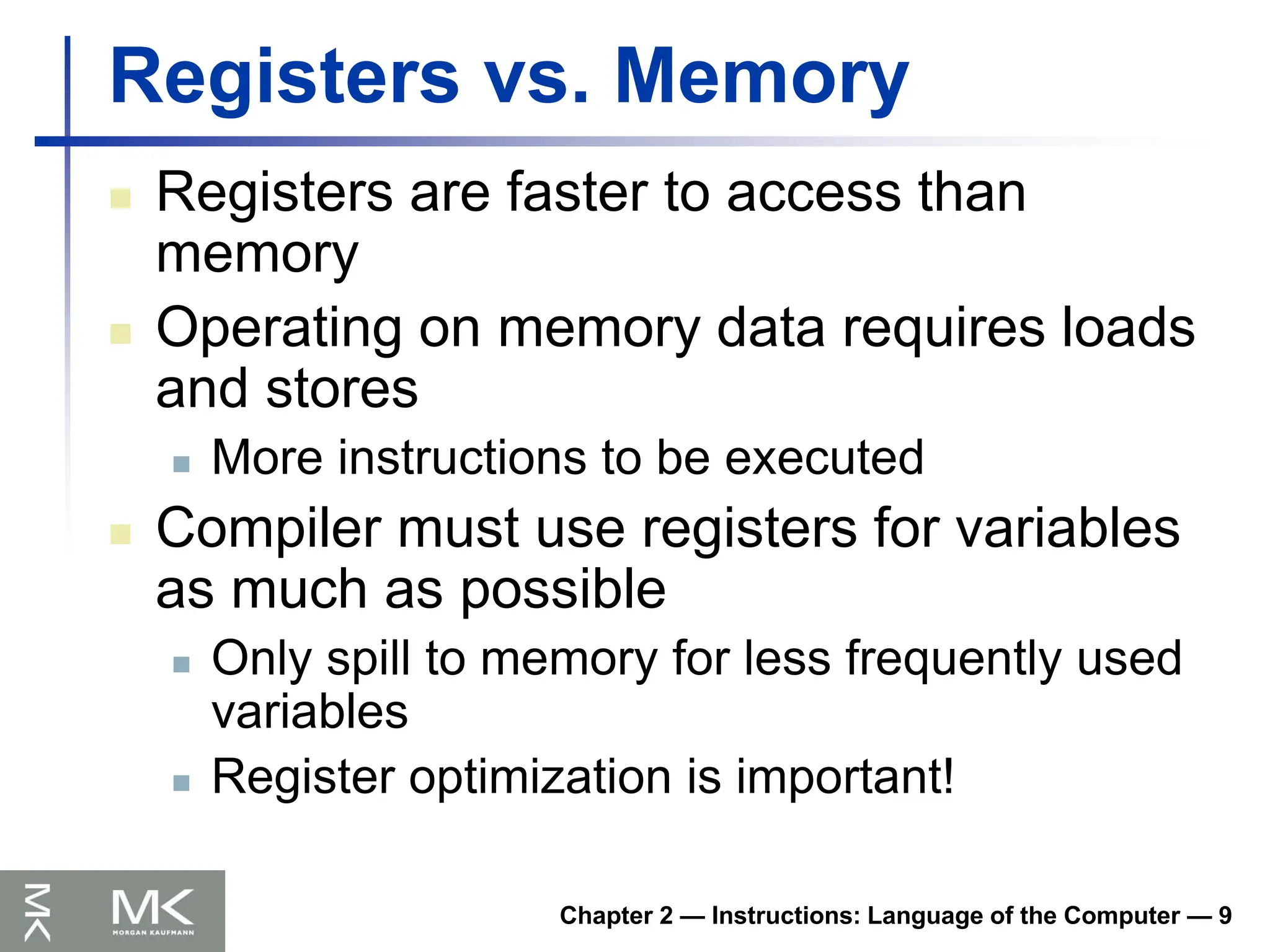
Registers vs. Memory
Registers are faster to access than
memory
Operating on memory data requires loads
and stores
More instructions to be executed
Compiler must use registers for variables
as much as possible
Only spill to memory for less frequently used
variables
Register optimization is important!
54.
Chapter 2 —Instructions: Language of the Computer — 10
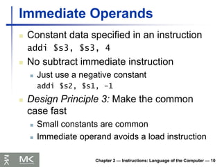
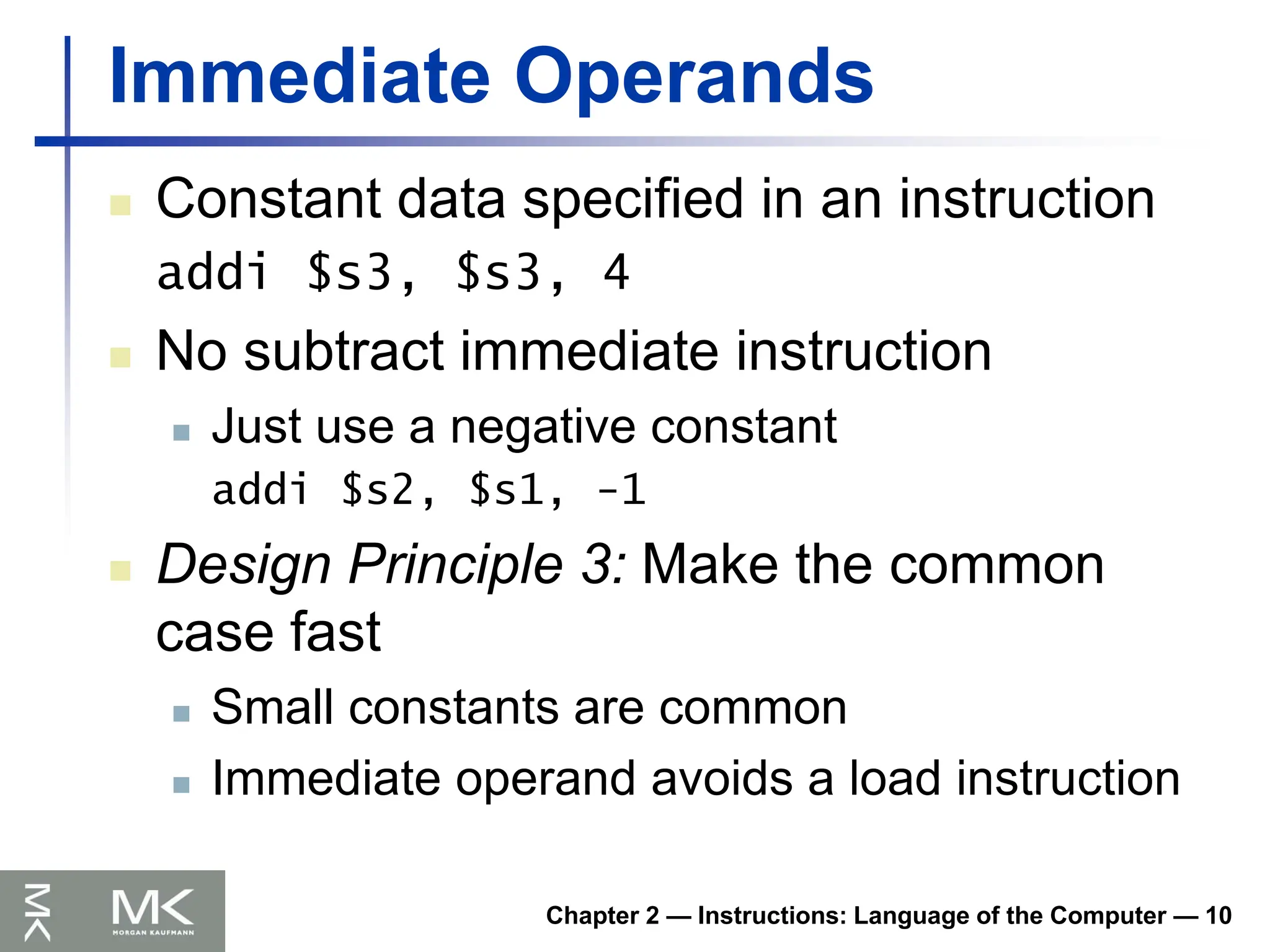
Immediate Operands
Constant data specified in an instruction
addi $s3, $s3, 4
No subtract immediate instruction
Just use a negative constant
addi $s2, $s1, -1
Design Principle 3: Make the common
case fast
Small constants are common
Immediate operand avoids a load instruction
55.
Chapter 2 —Instructions: Language of the Computer — 11
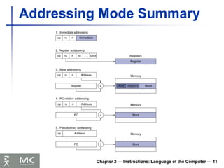
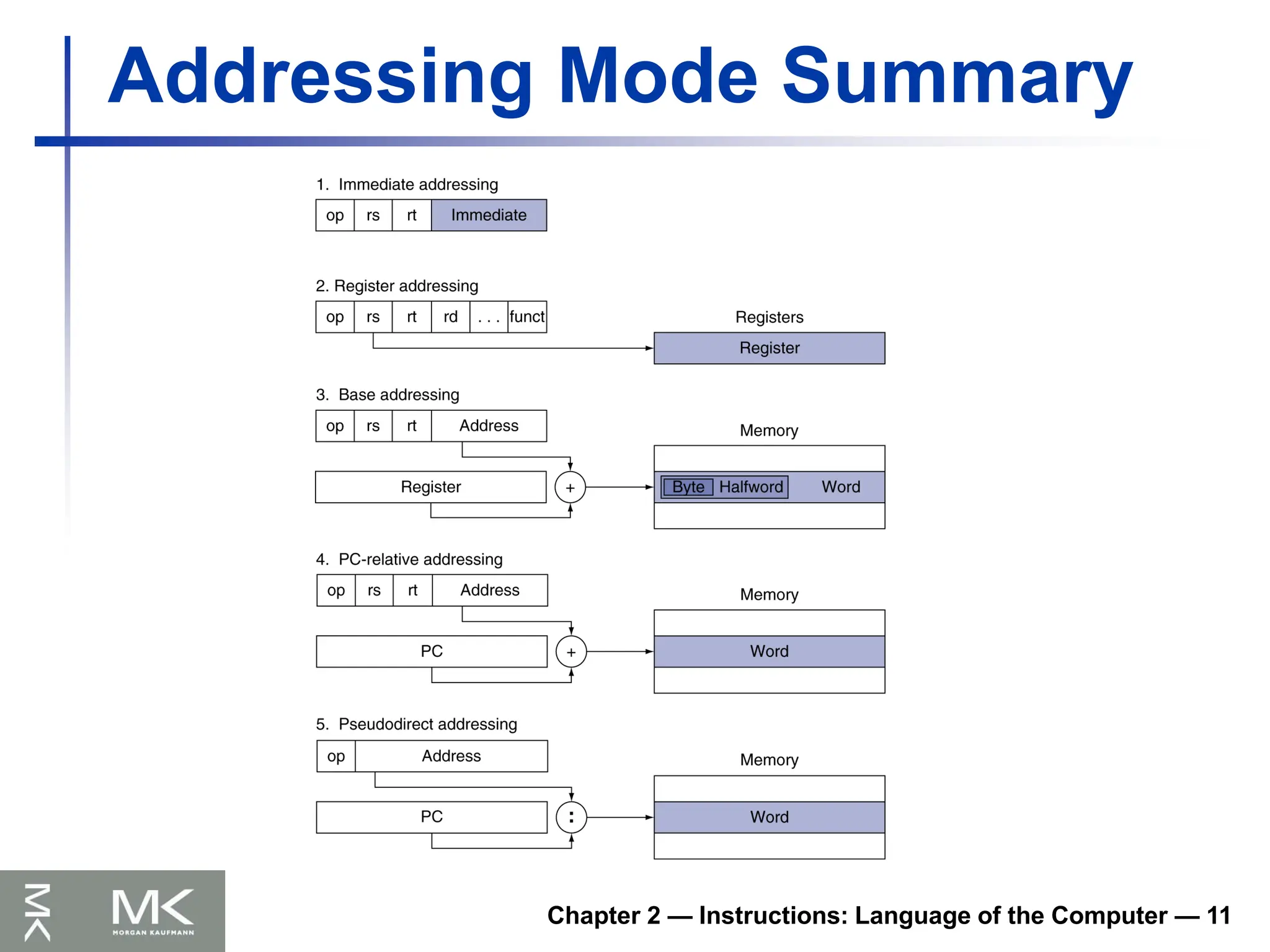
Addressing Mode Summary
56.
Chapter 2 —Instructions: Language of the Computer — 12
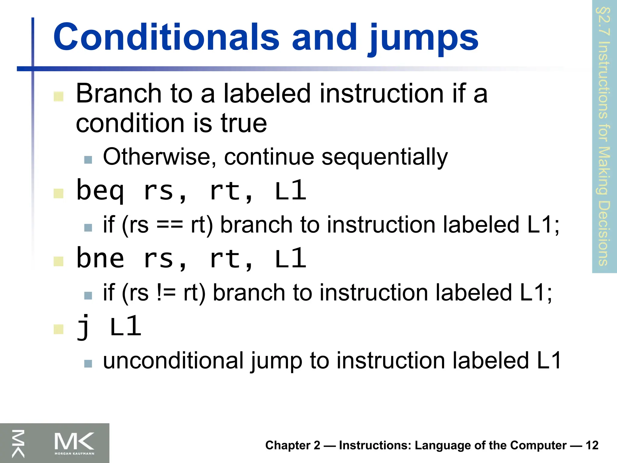
Conditionals and jumps
Branch to a labeled instruction if a
condition is true
Otherwise, continue sequentially
beq rs, rt, L1
if (rs == rt) branch to instruction labeled L1;
bne rs, rt, L1
if (rs != rt) branch to instruction labeled L1;
j L1
unconditional jump to instruction labeled L1
§2.7
Instructions
for
Making
Decisions
57.
Chapter 2 —Instructions: Language of the Computer — 13
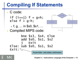
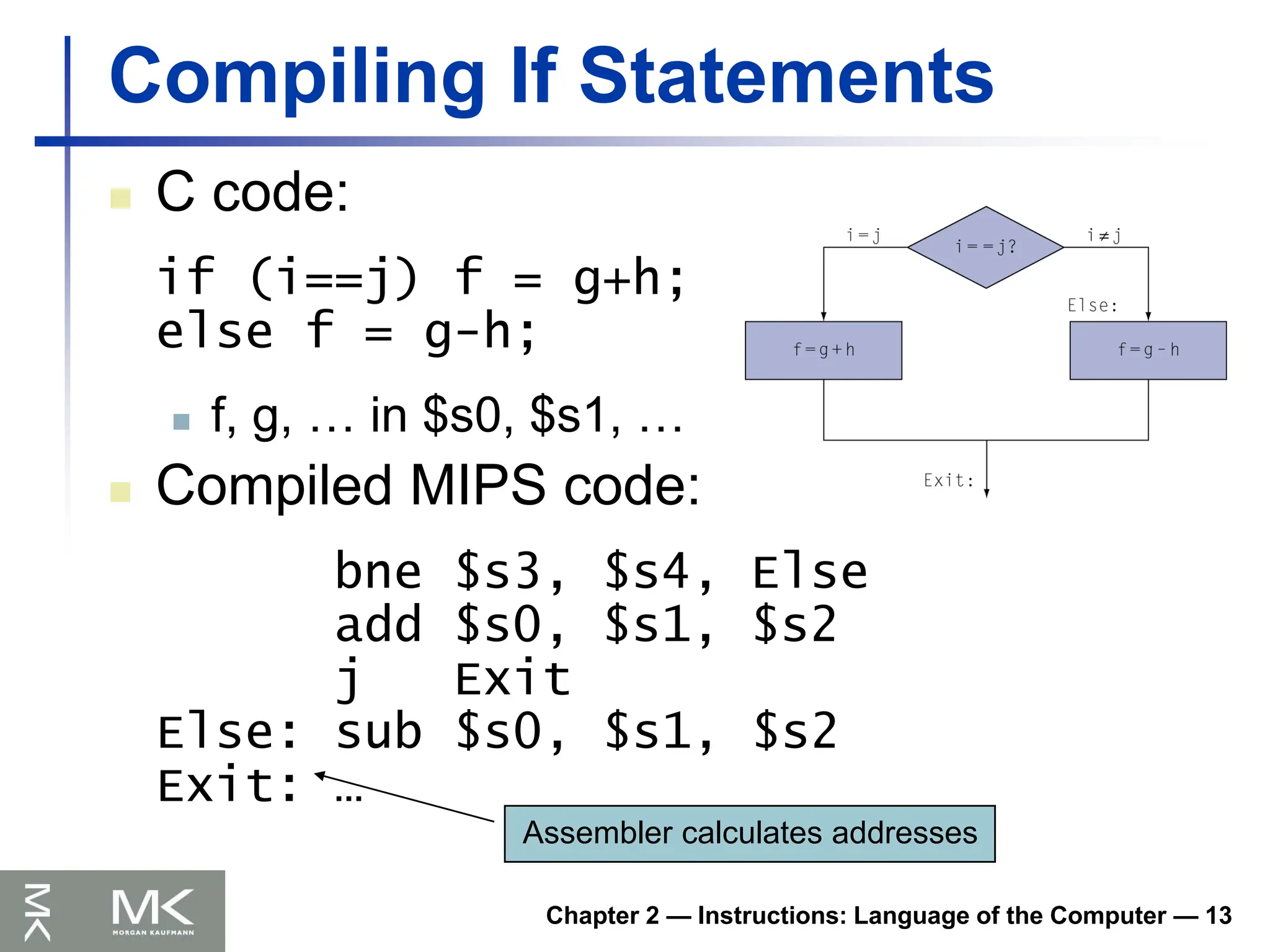
Compiling If Statements
C code:
if (i==j) f = g+h;
else f = g-h;
f, g, … in $s0, $s1, …
Compiled MIPS code:
bne $s3, $s4, Else
add $s0, $s1, $s2
j Exit
Else: sub $s0, $s1, $s2
Exit: …
Assembler calculates addresses
58.
Chapter 2 —Instructions: Language of the Computer — 14
Compiling Loop Statements
C code:
while (save[i] == k) i += 1;
i in $s3, k in $s5, address of save in $s6
Compiled MIPS code:
Loop: sll $t1, $s3, 2
add $t1, $t1, $s6
lw $t0, 0($t1)
bne $t0, $s5, Exit
addi $s3, $s3, 1
j Loop
Exit: …
59.
Chapter 2 —Instructions: Language of the Computer — 15
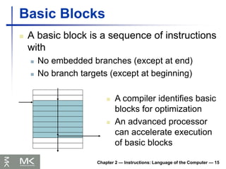
Basic Blocks
A basic block is a sequence of instructions
with
No embedded branches (except at end)
No branch targets (except at beginning)
A compiler identifies basic
blocks for optimization
An advanced processor
can accelerate execution
of basic blocks
60.
Chapter 2 —Instructions: Language of the Computer — 16
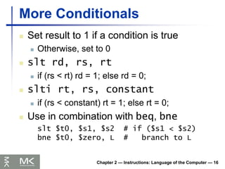
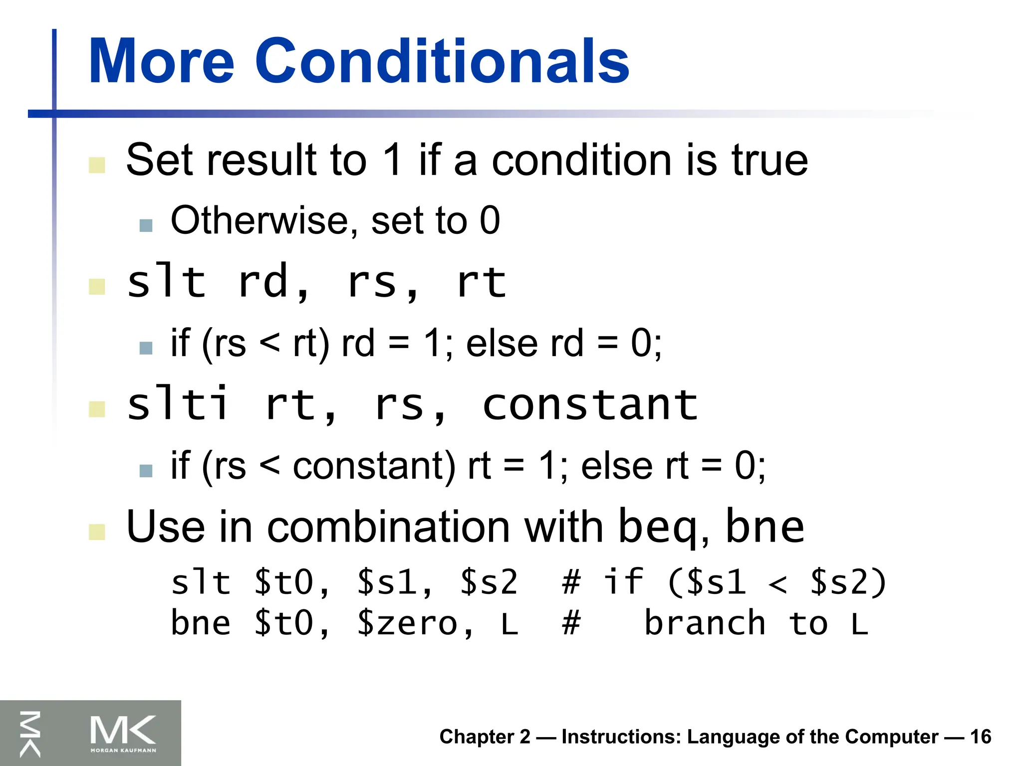
More Conditionals
Set result to 1 if a condition is true
Otherwise, set to 0
slt rd, rs, rt
if (rs < rt) rd = 1; else rd = 0;
slti rt, rs, constant
if (rs < constant) rt = 1; else rt = 0;
Use in combination with beq, bne
slt $t0, $s1, $s2 # if ($s1 < $s2)
bne $t0, $zero, L # branch to L
61.
Chapter 2 —Instructions: Language of the Computer — 17
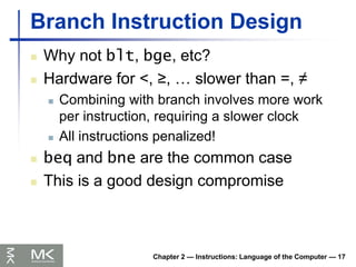
Branch Instruction Design
Why not blt, bge, etc?
Hardware for <, ≥, … slower than =, ≠
Combining with branch involves more work
per instruction, requiring a slower clock
All instructions penalized!
beq and bne are the common case
This is a good design compromise
62.
Chapter 2 —Instructions: Language of the Computer — 18
Procedure Calling
Steps required
1. Place parameters in registers
2. Transfer control to procedure
3. Acquire storage for procedure
4. Perform procedure’s operations
5. Place result in register for caller
6. Return to place of call
§2.8
Supporting
Procedures
in
Computer
Hardware
63.
Chapter 2 —Instructions: Language of the Computer — 19
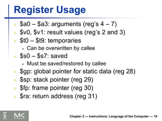
Register Usage
$a0 – $a3: arguments (reg’s 4 – 7)
$v0, $v1: result values (reg’s 2 and 3)
$t0 – $t9: temporaries
Can be overwritten by callee
$s0 – $s7: saved
Must be saved/restored by callee
$gp: global pointer for static data (reg 28)
$sp: stack pointer (reg 29)
$fp: frame pointer (reg 30)
$ra: return address (reg 31)
64.
Chapter 2 —Instructions: Language of the Computer — 20
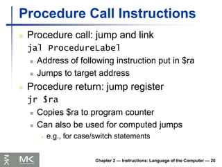
Procedure Call Instructions
Procedure call: jump and link
jal ProcedureLabel
Address of following instruction put in $ra
Jumps to target address
Procedure return: jump register
jr $ra
Copies $ra to program counter
Can also be used for computed jumps
e.g., for case/switch statements
65.
Chapter 2 —Instructions: Language of the Computer — 21
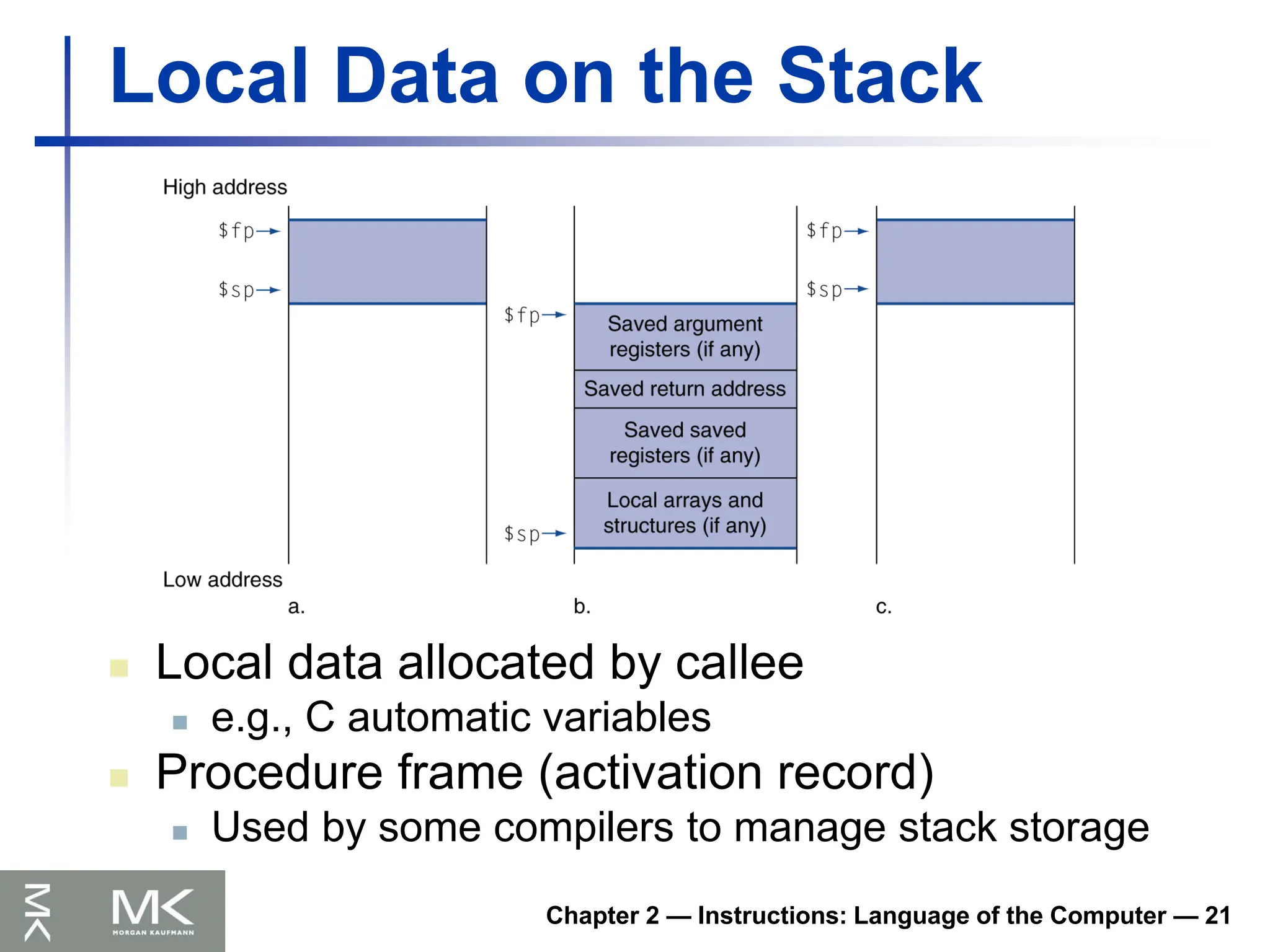
Local Data on the Stack
Local data allocated by callee
e.g., C automatic variables
Procedure frame (activation record)
Used by some compilers to manage stack storage
66.
Chapter 2 —Instructions: Language of the Computer — 22
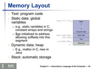
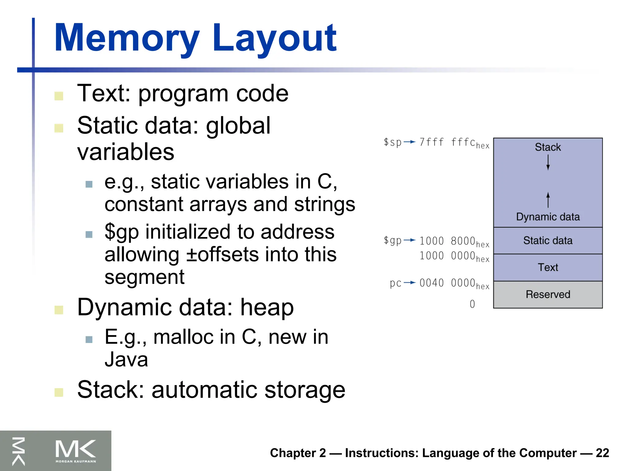
Memory Layout
Text: program code
Static data: global
variables
e.g., static variables in C,
constant arrays and strings
$gp initialized to address
allowing ±offsets into this
segment
Dynamic data: heap
E.g., malloc in C, new in
Java
Stack: automatic storage
67.
Chapter 2 —Instructions: Language of the Computer — 23
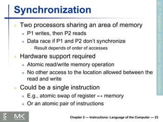
Synchronization
Two processors sharing an area of memory
P1 writes, then P2 reads
Data race if P1 and P2 don’t synchronize
Result depends of order of accesses
Hardware support required
Atomic read/write memory operation
No other access to the location allowed between the
read and write
Could be a single instruction
E.g., atomic swap of register ↔ memory
Or an atomic pair of instructions
§2.11
Parallelism
and
Instructions:
Synchronization
68.
Chapter 2 —Instructions: Language of the Computer — 24
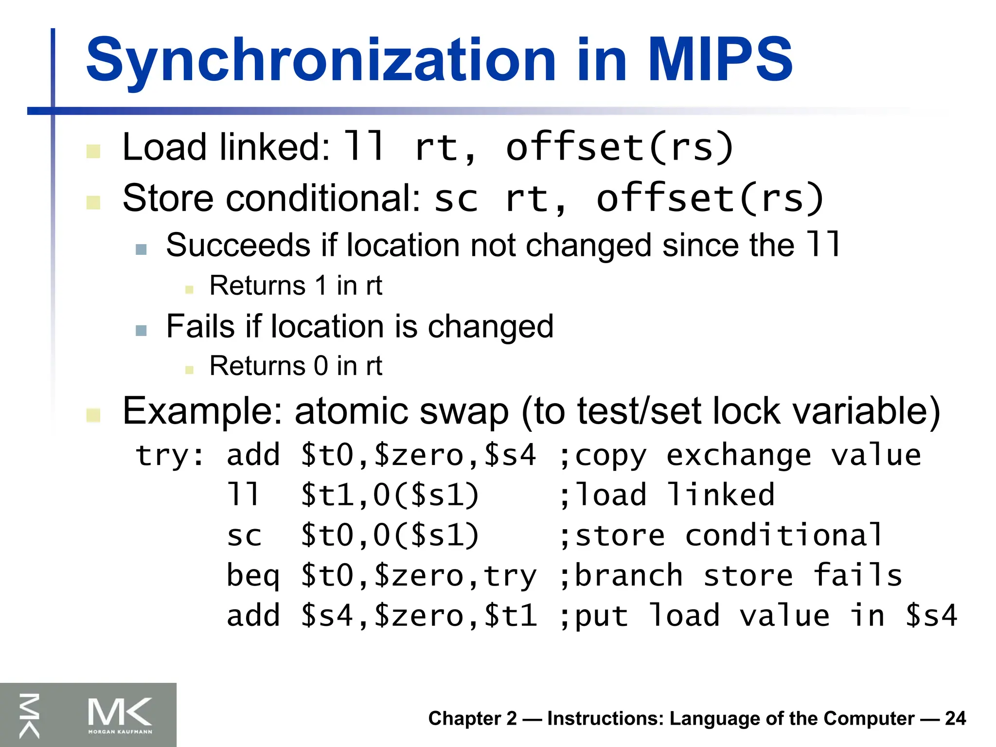
Synchronization in MIPS
Load linked: ll rt, offset(rs)
Store conditional: sc rt, offset(rs)
Succeeds if location not changed since the ll
Returns 1 in rt
Fails if location is changed
Returns 0 in rt
Example: atomic swap (to test/set lock variable)
try: add $t0,$zero,$s4 ;copy exchange value
ll $t1,0($s1) ;load linked
sc $t0,0($s1) ;store conditional
beq $t0,$zero,try ;branch store fails
add $s4,$zero,$t1 ;put load value in $s4
69.
Chapter 3 —Arithmetic for Computers — 25
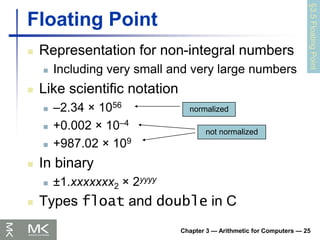
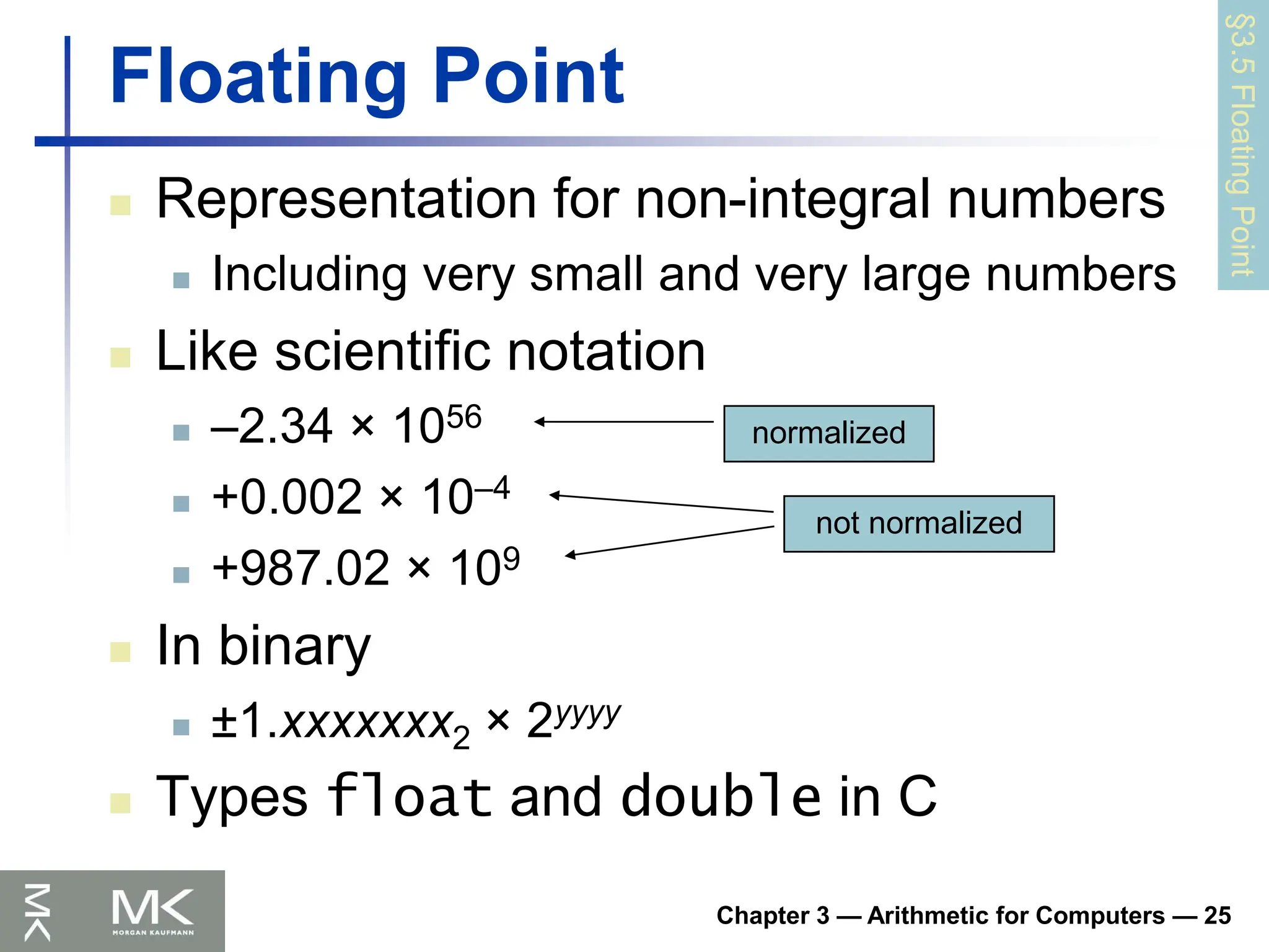
Floating Point
Representation for non-integral numbers
Including very small and very large numbers
Like scientific notation
–2.34 × 1056
+0.002 × 10⁻⁴
+987.02 × 10⁹
In binary
±1.xxxxxxx2 × 2yyyy
Types float and double in C
normalized
not normalized
§3.5
Floating
Point
70.
Chapter 3 —Arithmetic for Computers — 26
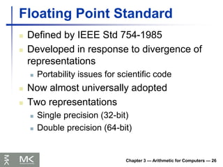
Floating Point Standard
Defined by IEEE Std 754-1985
Developed in response to divergence of
representations
Portability issues for scientific code
Now almost universally adopted
Two representations
Single precision (32-bit)
Double precision (64-bit)
71.
Chapter 3 —Arithmetic for Computers — 27
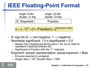
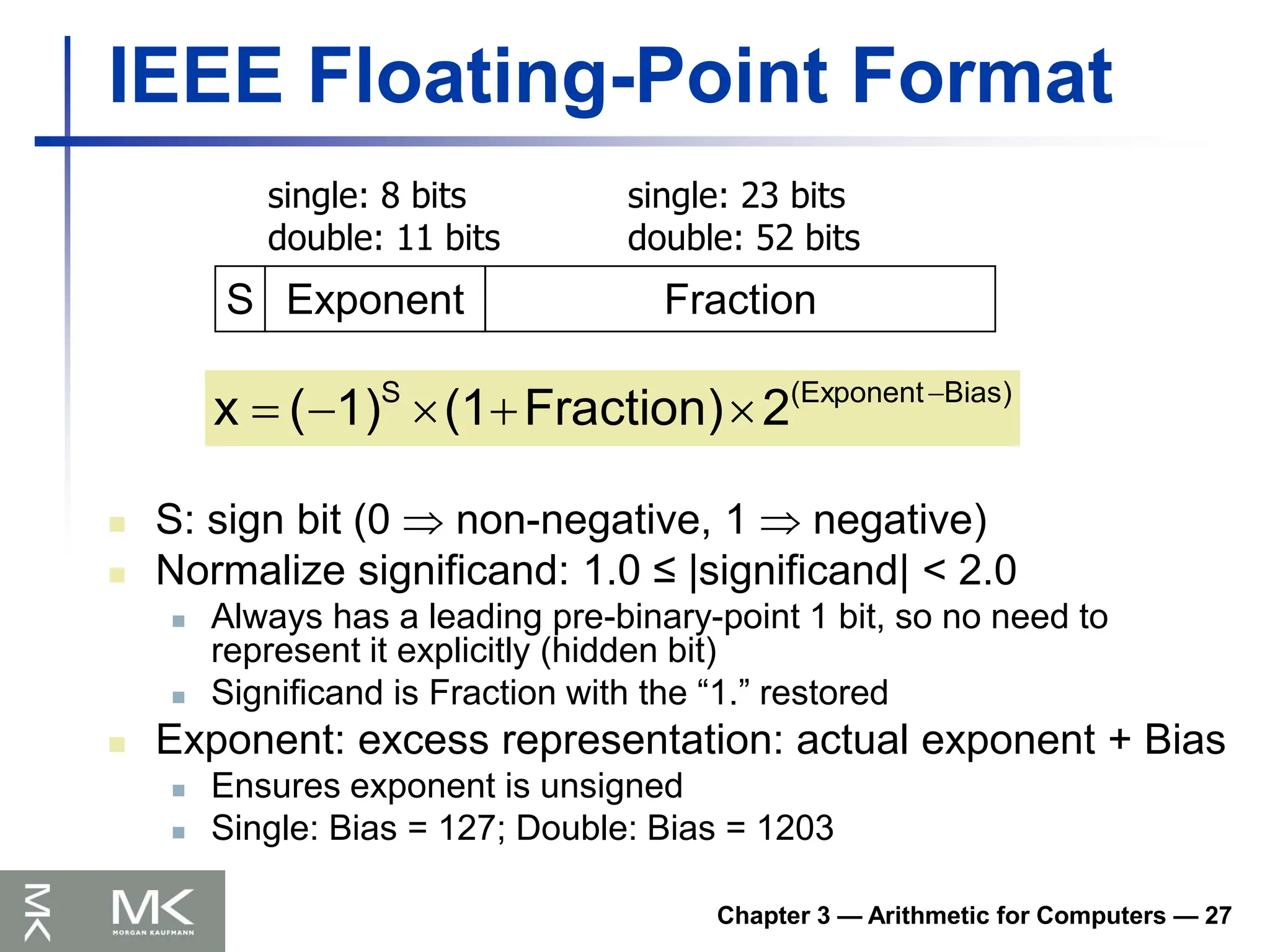
IEEE Floating-Point Format
S: sign bit (0 non-negative, 1 negative)
Normalize significand: 1.0 ≤ |significand| < 2.0
Always has a leading pre-binary-point 1 bit, so no need to
represent it explicitly (hidden bit)
Significand is Fraction with the “1.” restored
Exponent: excess representation: actual exponent + Bias
Ensures exponent is unsigned
Single: Bias = 127; Double: Bias = 1203
S Exponent Fraction
single: 8 bits
double: 11 bits
single: 23 bits
double: 52 bits
Bias)
(Exponent
S
2
Fraction)
(1
1)
(
x
72.
Chapter 3 —Arithmetic for Computers — 28
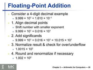
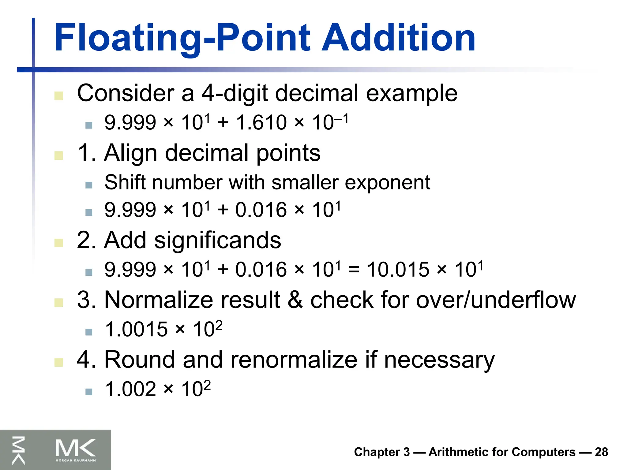
Floating-Point Addition
Consider a 4-digit decimal example
9.999 × 101 + 1.610 × 10⁻¹
1. Align decimal points
Shift number with smaller exponent
9.999 × 101 + 0.016 × 101
2. Add significands
9.999 × 101 + 0.016 × 101 = 10.015 × 101
3. Normalize result & check for over/underflow
1.0015 × 10²
4. Round and renormalize if necessary
1.002 × 10²
73.
Chapter 3 —Arithmetic for Computers — 29
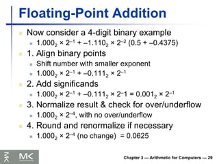
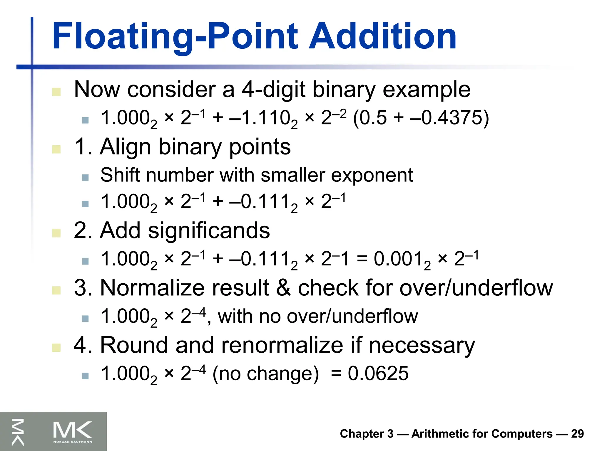
Floating-Point Addition
Now consider a 4-digit binary example
1.0002 × 2–1 + –1.1102 × 2–2 (0.5 + –0.4375)
1. Align binary points
Shift number with smaller exponent
1.0002 × 2–1 + –0.1112 × 2–1
2. Add significands
1.0002 × 2–1 + –0.1112 × 2–1 = 0.0012 × 2–1
3. Normalize result & check for over/underflow
1.0002 × 2–4, with no over/underflow
4. Round and renormalize if necessary
1.0002 × 2–4 (no change) = 0.0625
74.
Chapter 3 —Arithmetic for Computers — 30
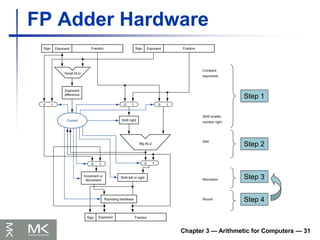
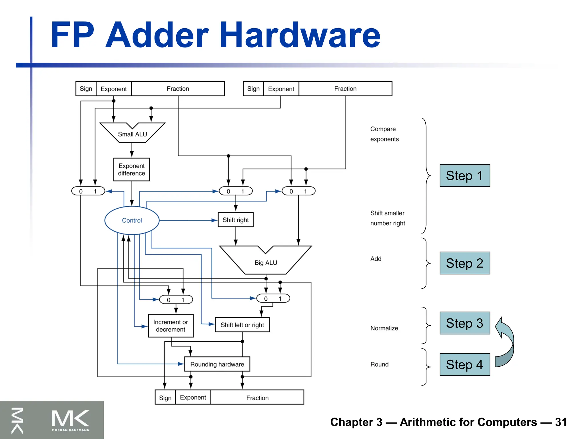
FP Adder Hardware
Much more complex than integer adder
Doing it in one clock cycle would take too
long
Much longer than integer operations
Slower clock would penalize all instructions
FP adder usually takes several cycles
Can be pipelined
Chapter 3 —Arithmetic for Computers — 32
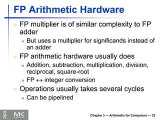
FP Arithmetic Hardware
FP multiplier is of similar complexity to FP
adder
But uses a multiplier for significands instead of
an adder
FP arithmetic hardware usually does
Addition, subtraction, multiplication, division,
reciprocal, square-root
FP integer conversion
Operations usually takes several cycles
Can be pipelined
77.
Chapter 3 —Arithmetic for Computers — 33
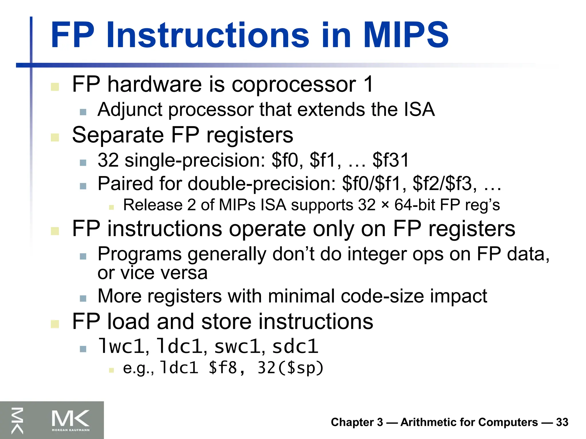
FP Instructions in MIPS
FP hardware is coprocessor 1
Adjunct processor that extends the ISA
Separate FP registers
32 single-precision: $f0, $f1, … $f31
Paired for double-precision: $f0/$f1, $f2/$f3, …
Release 2 of MIPs ISA supports 32 × 64-bit FP reg’s
FP instructions operate only on FP registers
Programs generally don’t do integer ops on FP data,
or vice versa
More registers with minimal code-size impact
FP load and store instructions
lwc1, ldc1, swc1, sdc1
e.g., ldc1 $f8, 32($sp)
78.
Chapter 3 —Arithmetic for Computers — 34
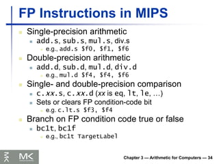
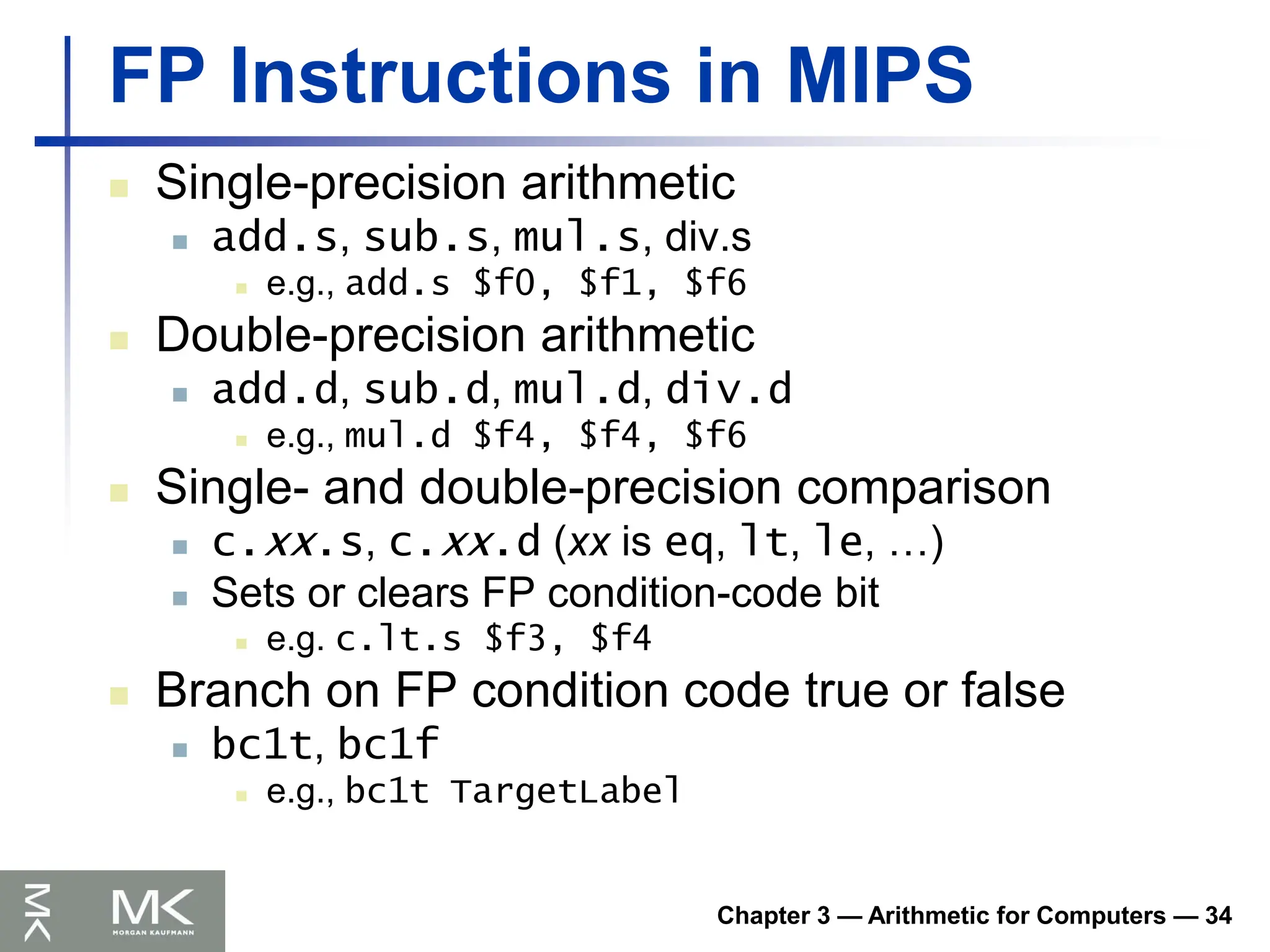
FP Instructions in MIPS
Single-precision arithmetic
add.s, sub.s, mul.s, div.s
e.g., add.s $f0, $f1, $f6
Double-precision arithmetic
add.d, sub.d, mul.d, div.d
e.g., mul.d $f4, $f4, $f6
Single- and double-precision comparison
c.xx.s, c.xx.d (xx is eq, lt, le, …)
Sets or clears FP condition-code bit
e.g. c.lt.s $f3, $f4
Branch on FP condition code true or false
bc1t, bc1f
e.g., bc1t TargetLabel
79.
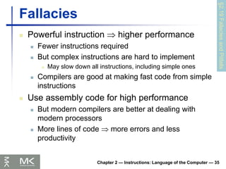
Chapter 2 —Instructions: Language of the Computer — 35
Fallacies
Powerful instruction higher performance
Fewer instructions required
But complex instructions are hard to implement
May slow down all instructions, including simple ones
Compilers are good at making fast code from simple
instructions
Use assembly code for high performance
But modern compilers are better at dealing with
modern processors
More lines of code more errors and less
productivity
§2.19
Fallacies
and
Pitfalls
80.
Chapter 2 —Instructions: Language of the Computer — 36
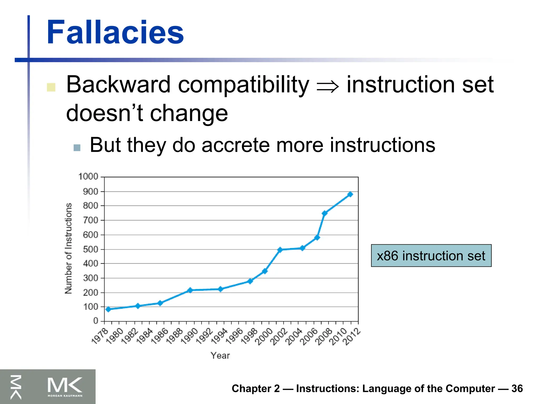
Fallacies
Backward compatibility instruction set
doesn’t change
But they do accrete more instructions
x86 instruction set
81.
Chapter 2 —Instructions: Language of the Computer — 37
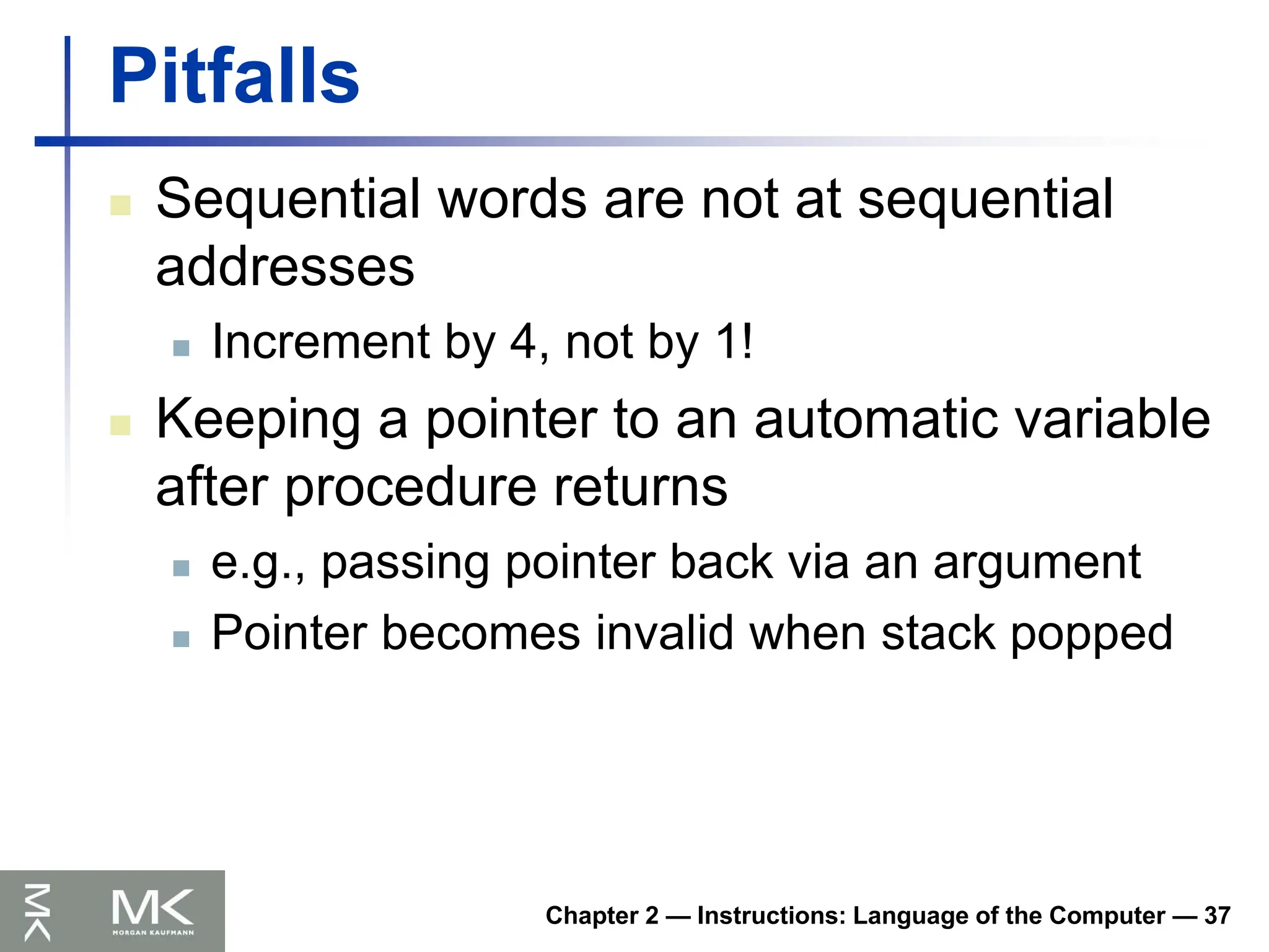
Pitfalls
Sequential words are not at sequential
addresses
Increment by 4, not by 1!
Keeping a pointer to an automatic variable
after procedure returns
e.g., passing pointer back via an argument
Pointer becomes invalid when stack popped
82.
Chapter 2 —Instructions: Language of the Computer — 38
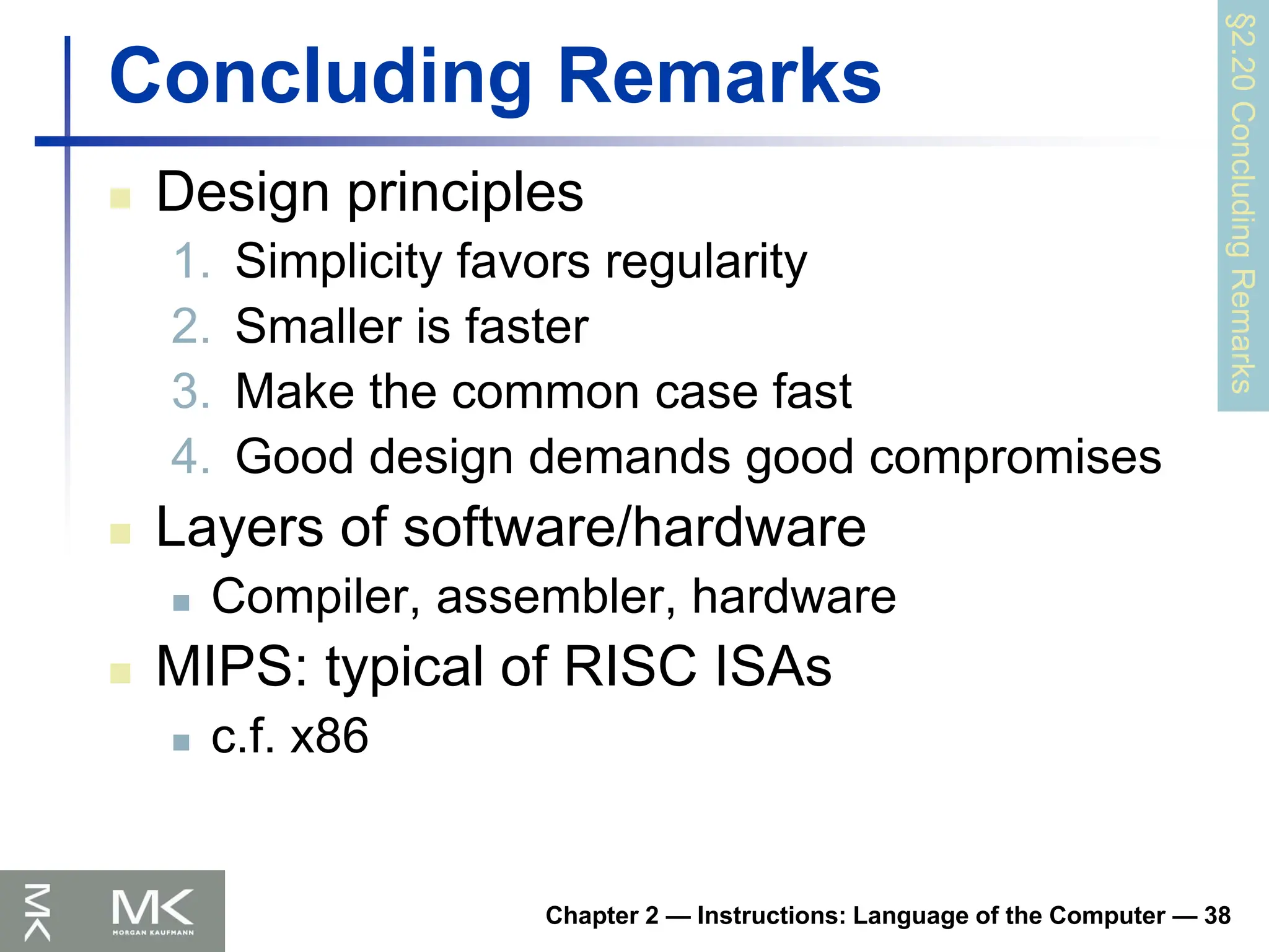
Concluding Remarks
Design principles
1. Simplicity favors regularity
2. Smaller is faster
3. Make the common case fast
4. Good design demands good compromises
Layers of software/hardware
Compiler, assembler, hardware
MIPS: typical of RISC ISAs
c.f. x86
§2.20
Concluding
Remarks
83.
Chapter 2 —Instructions: Language of the Computer — 39
Concluding Remarks
Measure MIPS instruction executions in
benchmark programs
Consider making the common case fast
Consider compromises
Instruction class MIPS examples SPEC2006 Int SPEC2006 FP
Arithmetic add, sub, addi 16% 48%
Data transfer lw, sw, lb, lbu,
lh, lhu, sb, lui
35% 36%
Logical and, or, nor, andi,
ori, sll, srl
12% 4%
Cond. Branch beq, bne, slt,
slti, sltiu
34% 8%
Jump j, jr, jal 2% 0%
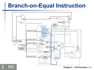
Chapter 4 —The Processor — 8
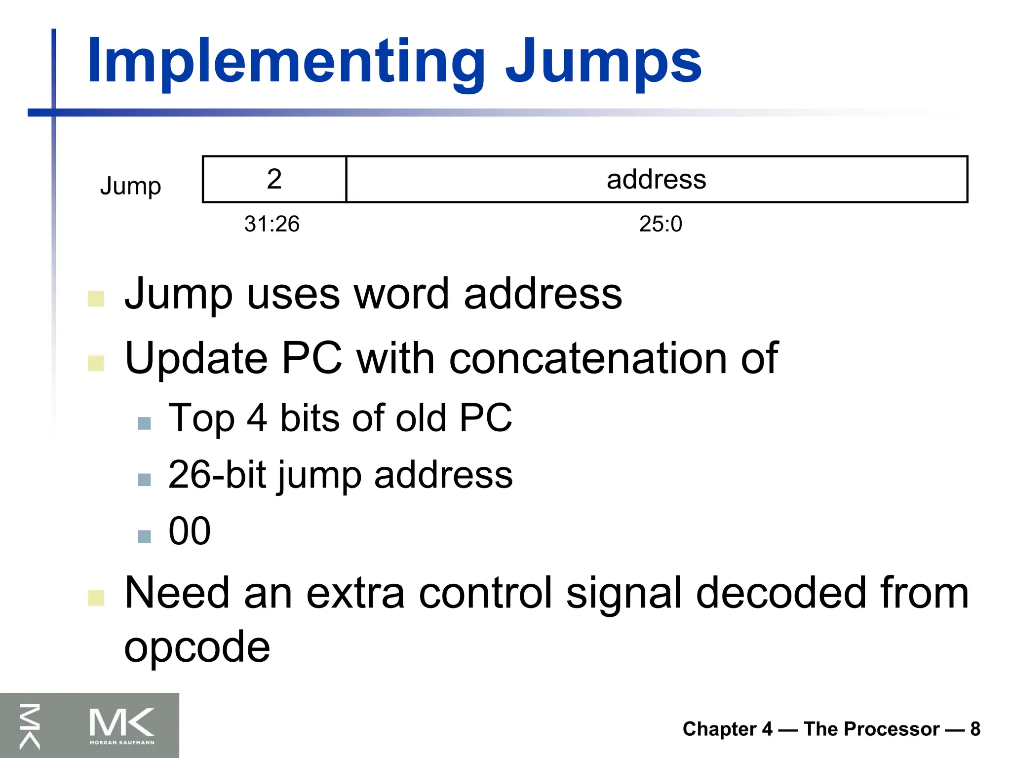
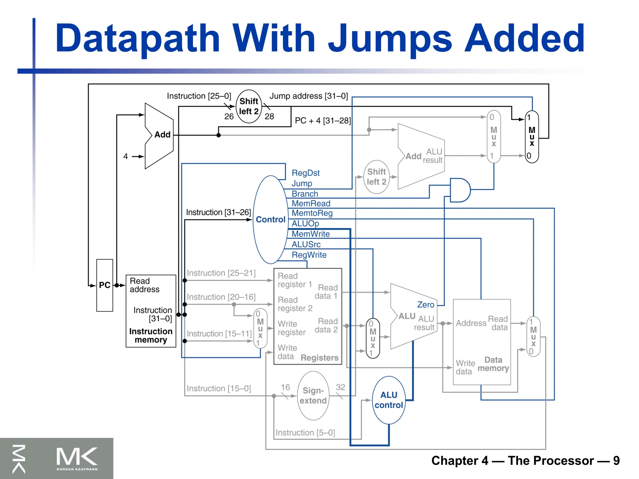
Implementing Jumps
Jump uses word address
Update PC with concatenation of
Top 4 bits of old PC
26-bit jump address
00
Need an extra control signal decoded from
opcode
2 address
31:26 25:0
Jump
92.
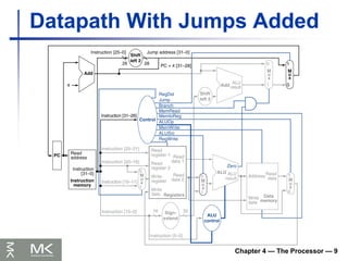
Chapter 4 —The Processor — 9
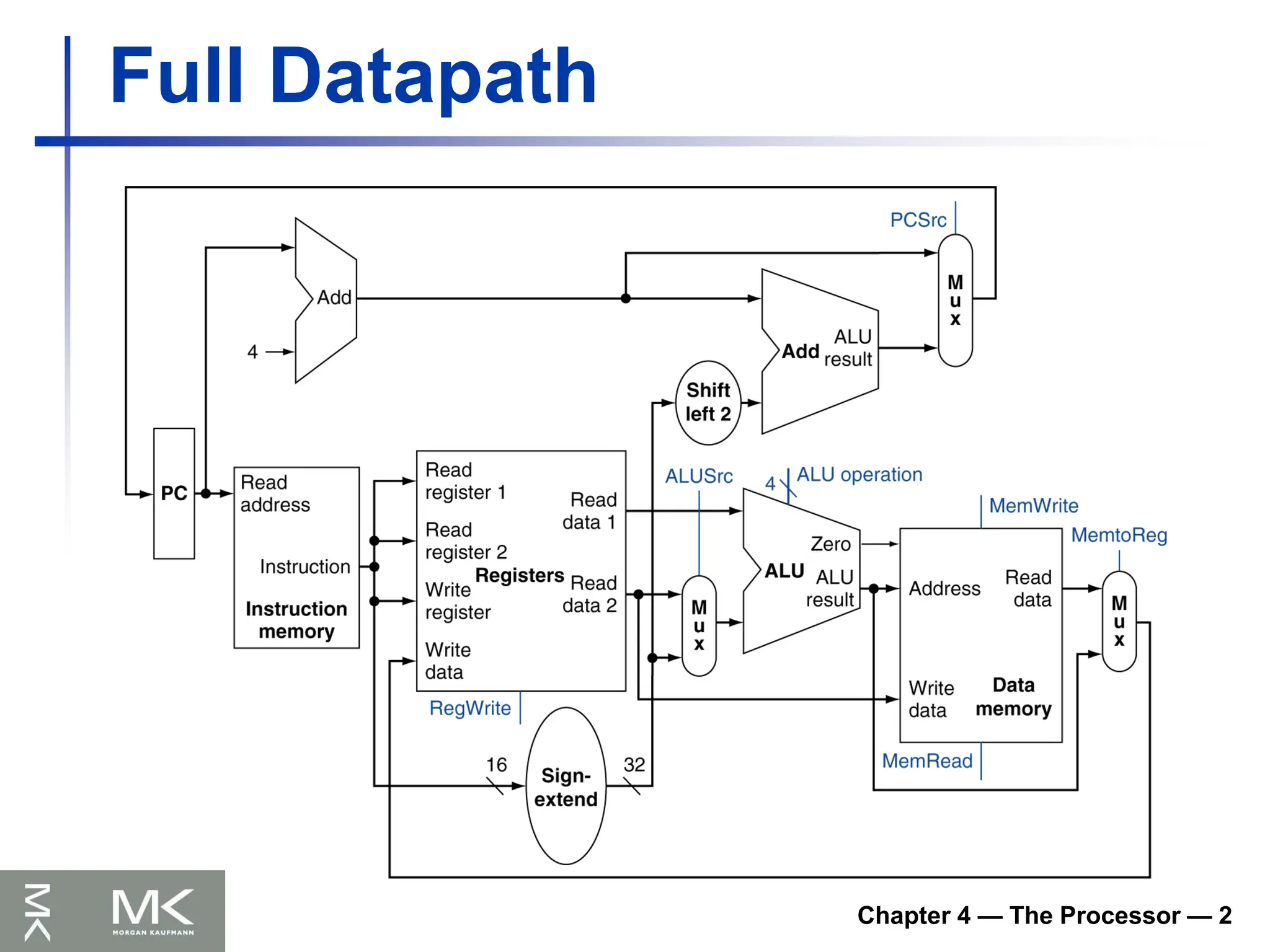
Datapath With Jumps Added
93.
Chapter 4 —The Processor — 10
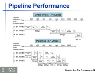
Performance Issues
Longest delay determines clock period
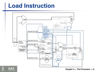
Critical path: load instruction
Instruction memory register file ALU
data memory register file
Not feasible to vary period for different
instructions
Violates design principle
Making the common case fast
Improve performance by pipelining
94.
Chapter 4 —The Processor — 11
MIPS Pipeline
Five stages, one step per stage
1. IF: Instruction fetch from memory
2. ID: Instruction decode & register read
3. EX: Execute operation or calculate address
4. MEM: Access memory operand
5. WB: Write result back to register
Chapter 4 —The Processor — 13
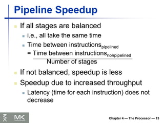
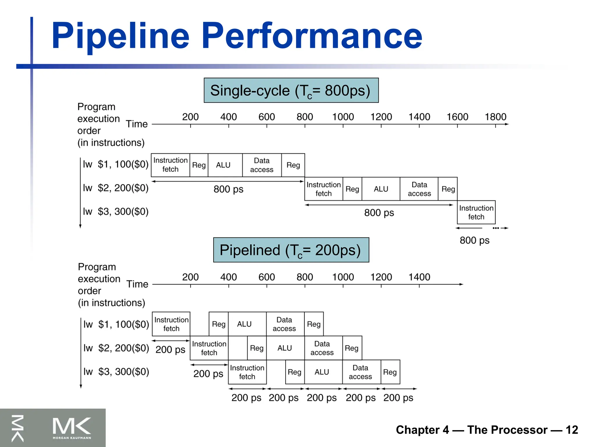
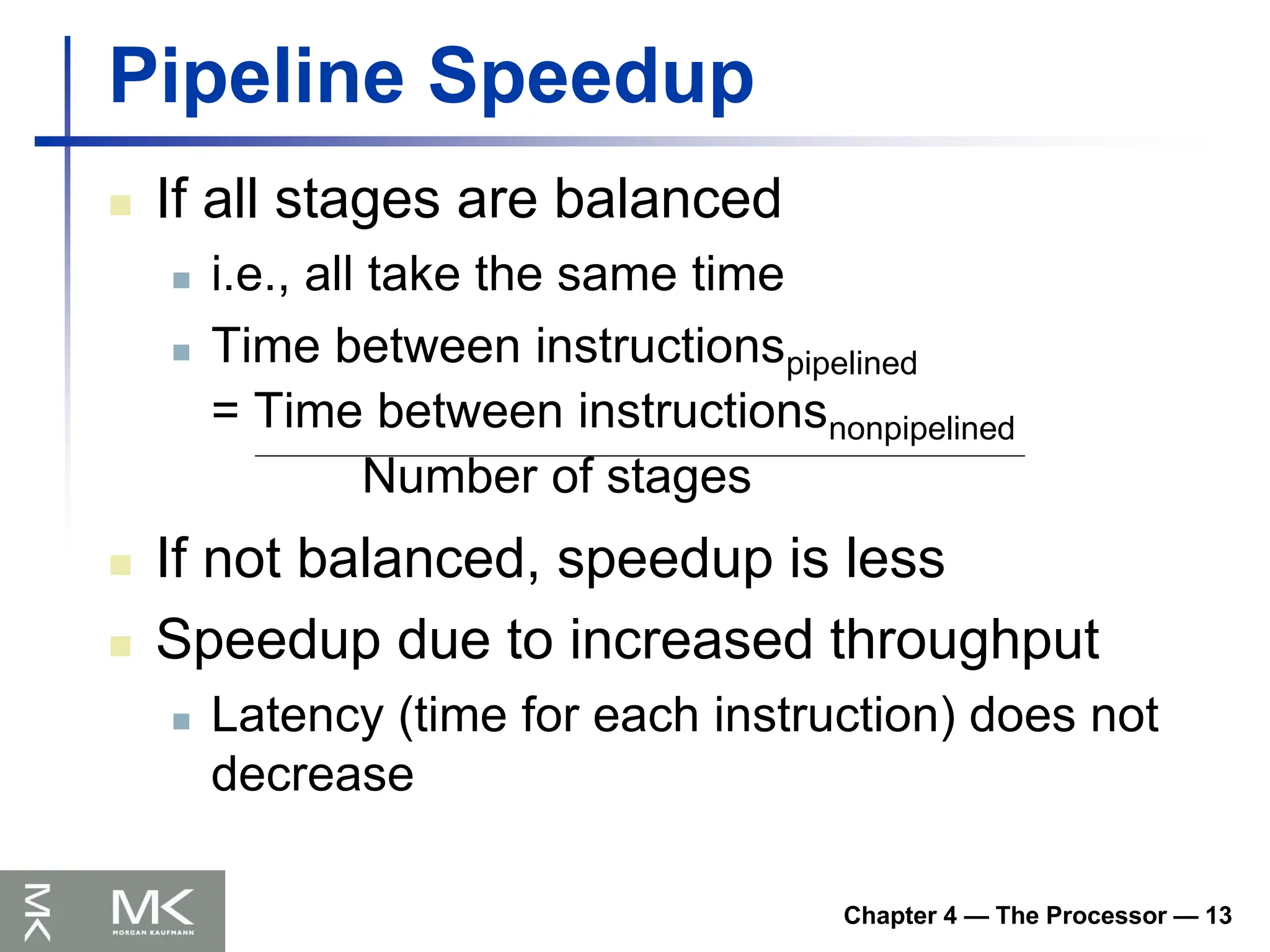
Pipeline Speedup
If all stages are balanced
i.e., all take the same time
Time between instructionspipelined
= Time between instructionsnonpipelined
Number of stages
If not balanced, speedup is less
Speedup due to increased throughput
Latency (time for each instruction) does not
decrease
97.
Chapter 4 —The Processor — 14
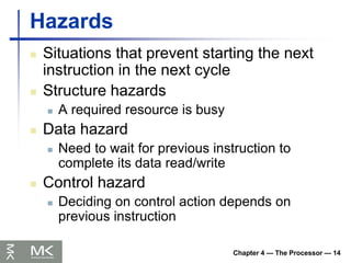
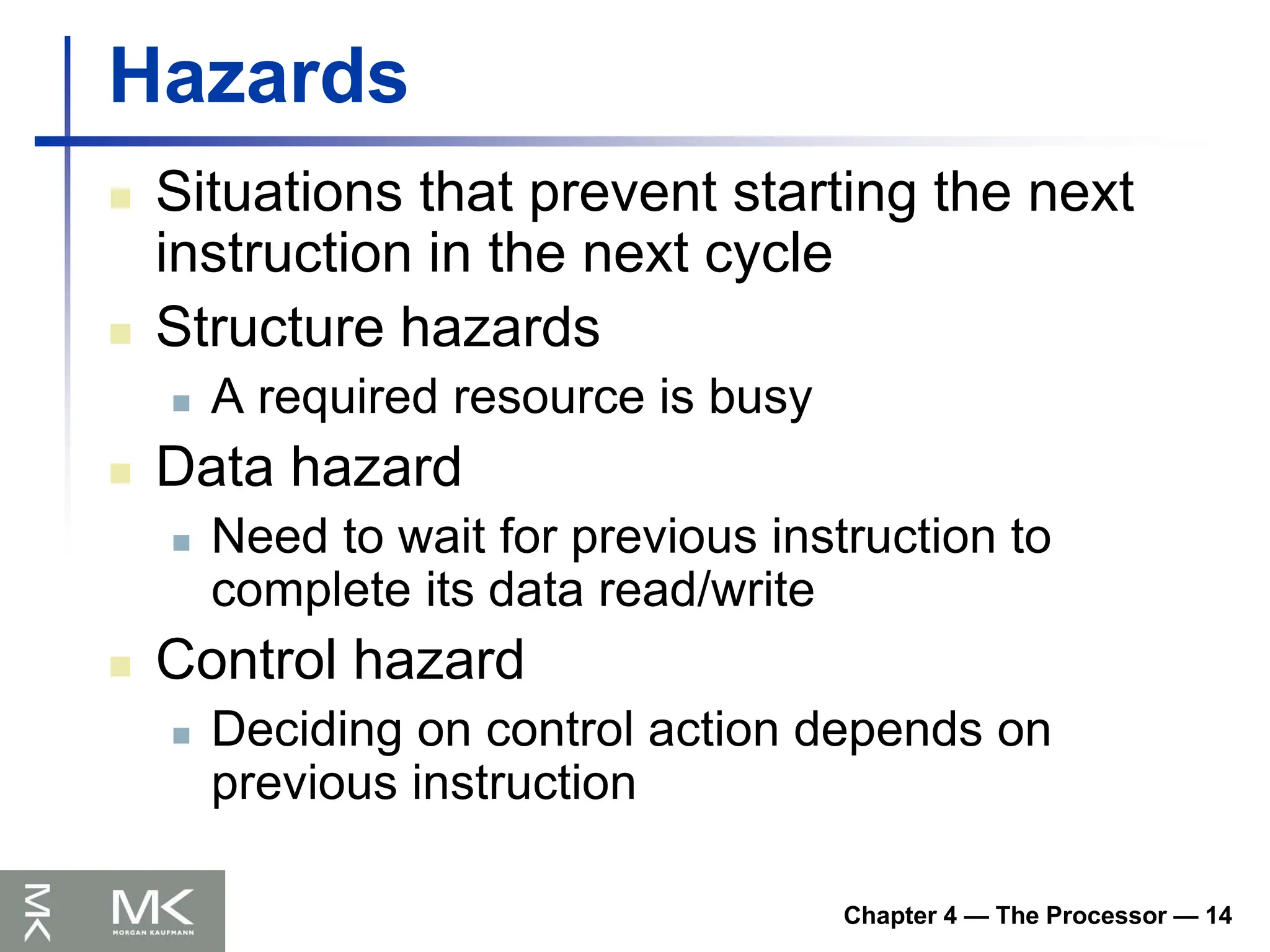
Hazards
Situations that prevent starting the next
instruction in the next cycle
Structure hazards
A required resource is busy
Data hazard
Need to wait for previous instruction to
complete its data read/write
Control hazard
Deciding on control action depends on
previous instruction
98.
Chapter 4 —The Processor — 15
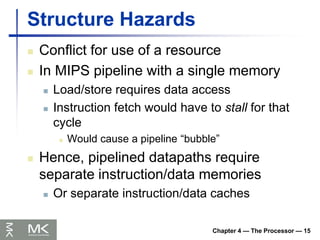
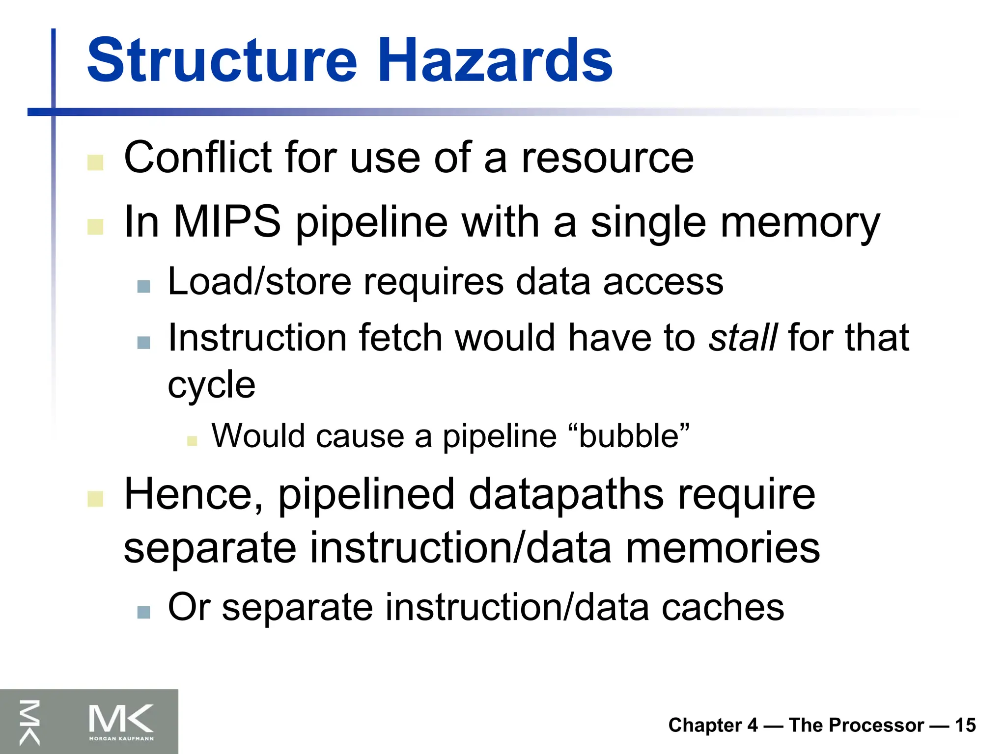
Structure Hazards
Conflict for use of a resource
In MIPS pipeline with a single memory
Load/store requires data access
Instruction fetch would have to stall for that
cycle
Would cause a pipeline “bubble”
Hence, pipelined datapaths require
separate instruction/data memories
Or separate instruction/data caches
99.
Chapter 4 —The Processor — 16
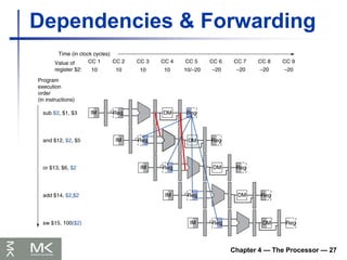
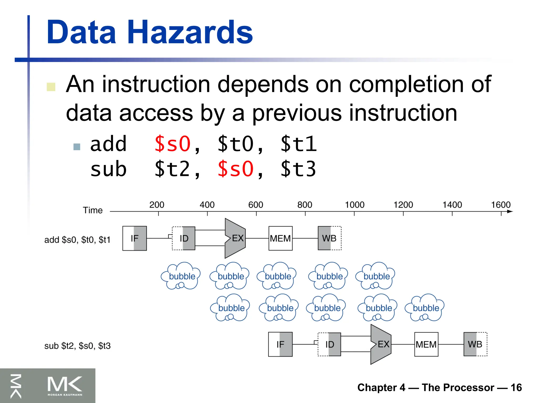
Data Hazards
An instruction depends on completion of
data access by a previous instruction
add $s0, $t0, $t1
sub $t2, $s0, $t3
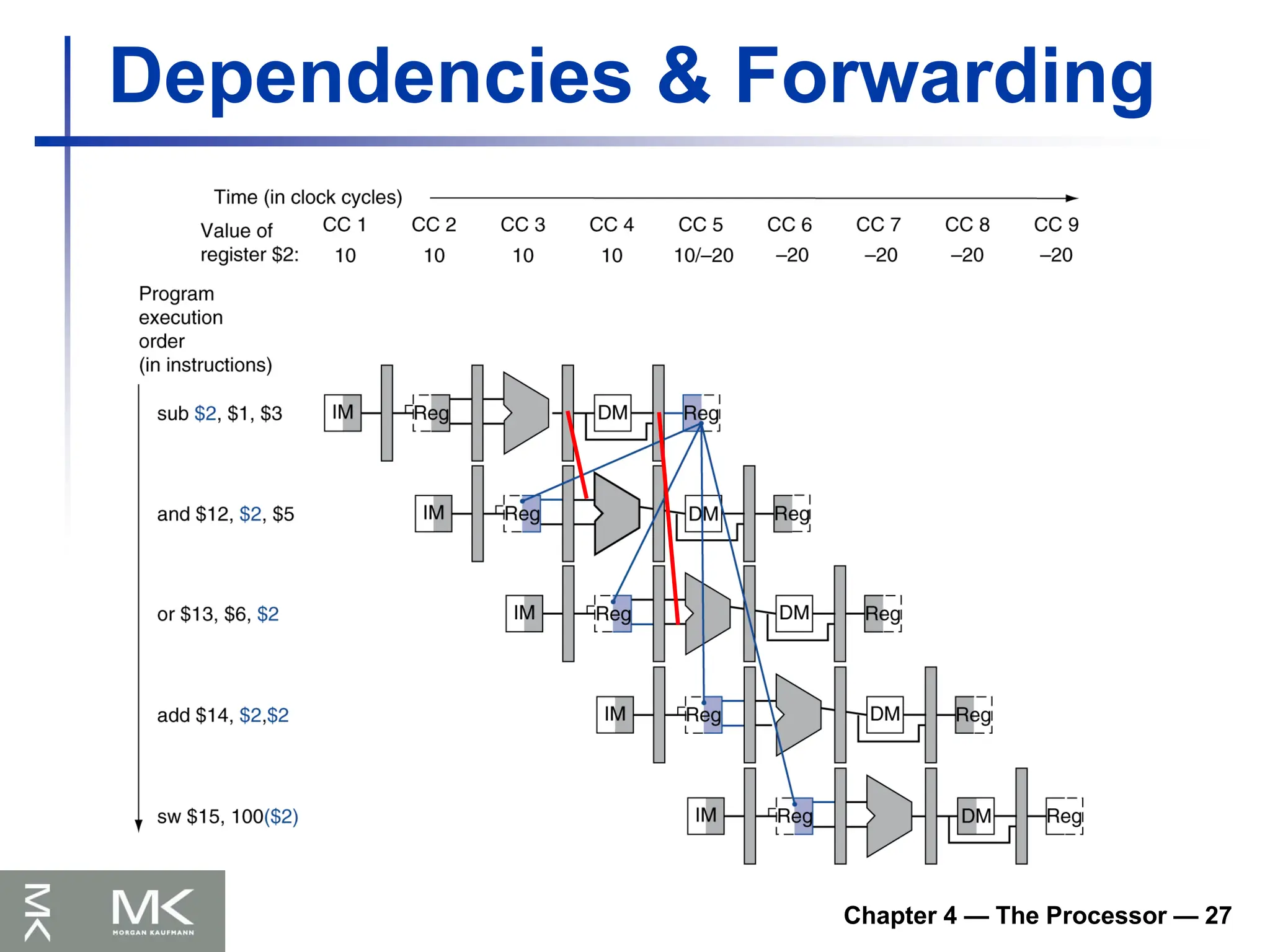
100.
Chapter 4 —The Processor — 17
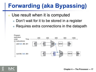
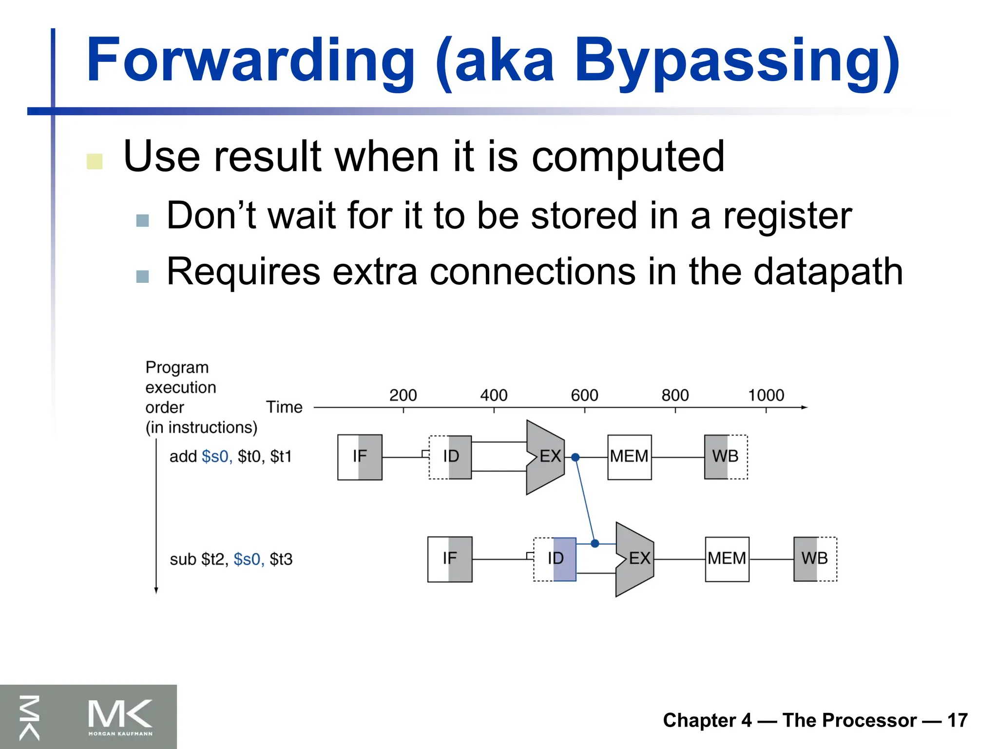
Forwarding (aka Bypassing)
Use result when it is computed
Don’t wait for it to be stored in a register
Requires extra connections in the datapath
101.
Chapter 4 —The Processor — 18
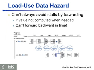
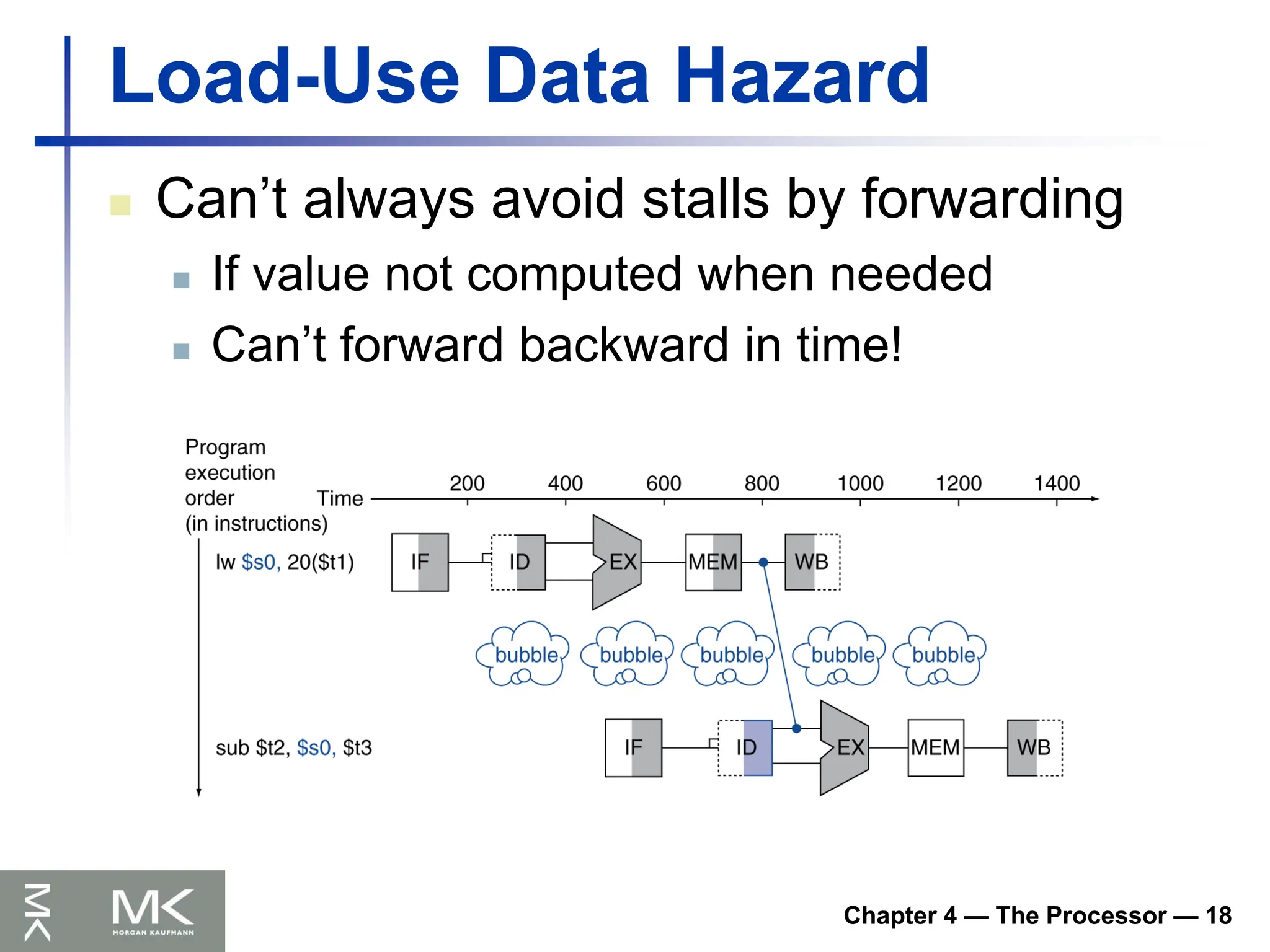
Load-Use Data Hazard
Can’t always avoid stalls by forwarding
If value not computed when needed
Can’t forward backward in time!
102.
Chapter 4 —The Processor — 19
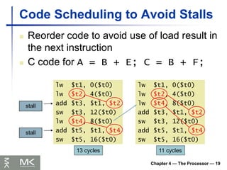
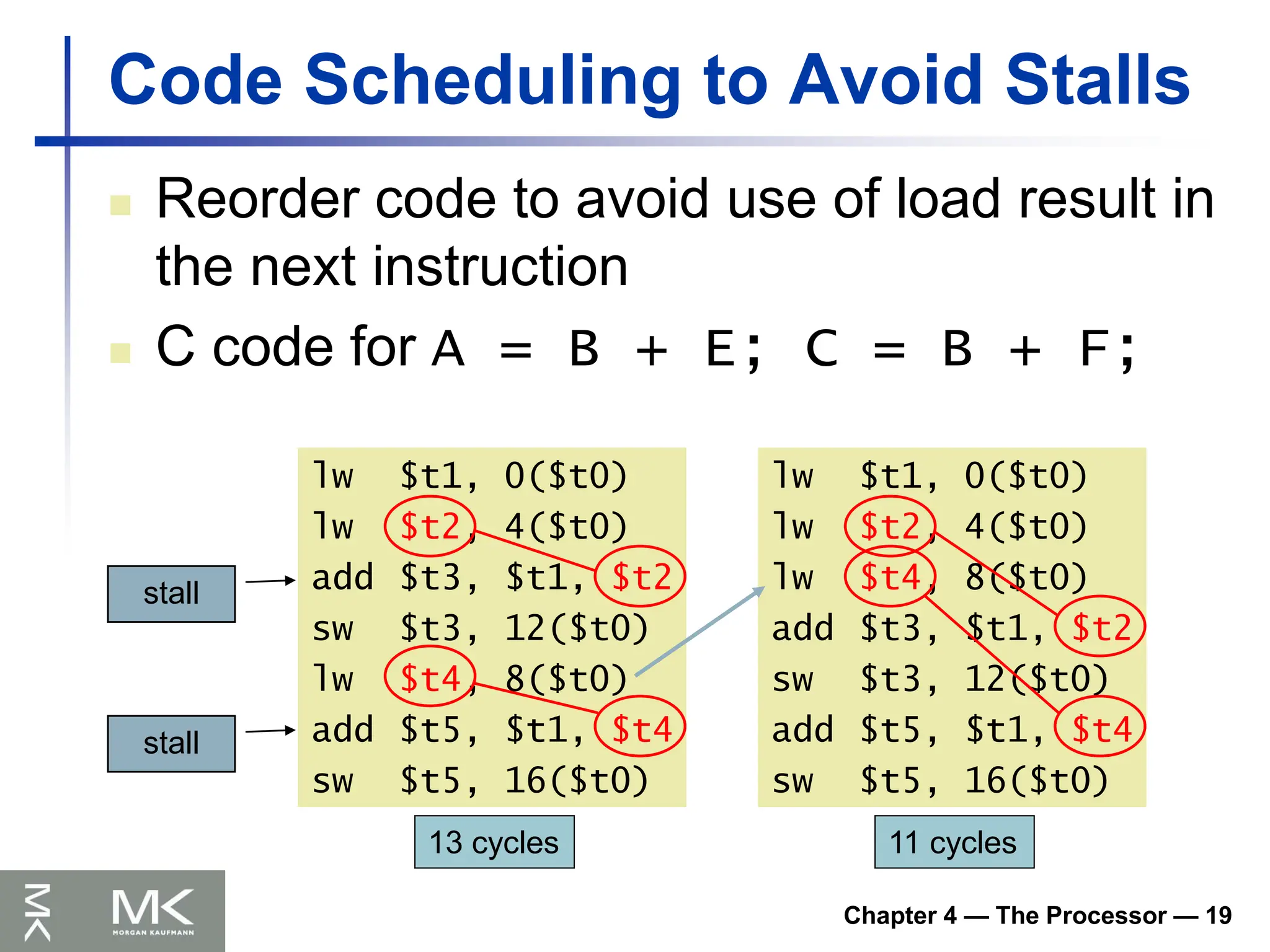
Code Scheduling to Avoid Stalls
Reorder code to avoid use of load result in
the next instruction
C code for A = B + E; C = B + F;
lw $t1, 0($t0)
lw $t2, 4($t0)
add $t3, $t1, $t2
sw $t3, 12($t0)
lw $t4, 8($t0)
add $t5, $t1, $t4
sw $t5, 16($t0)
stall
stall
lw $t1, 0($t0)
lw $t2, 4($t0)
lw $t4, 8($t0)
add $t3, $t1, $t2
sw $t3, 12($t0)
add $t5, $t1, $t4
sw $t5, 16($t0)
11 cycles
13 cycles
103.
Chapter 4 —The Processor — 20
Control Hazards
Branch determines flow of control
Fetching next instruction depends on branch
outcome
Pipeline can’t always fetch correct instruction
Still working on ID stage of branch
In MIPS pipeline
Need to compare registers and compute
target early in the pipeline
Add hardware to do it in ID stage
104.
Chapter 4 —The Processor — 21
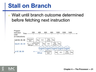
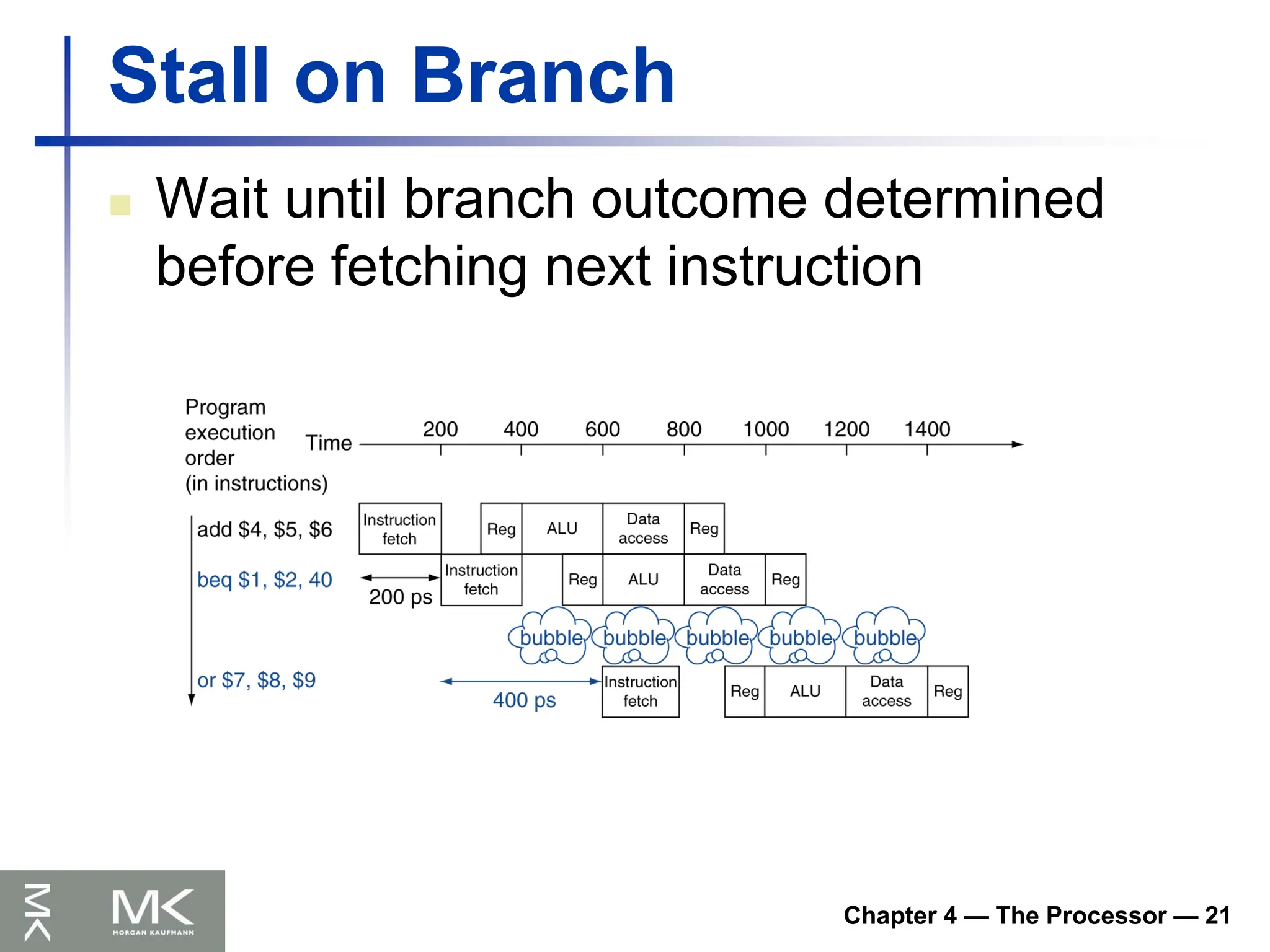
Stall on Branch
Wait until branch outcome determined
before fetching next instruction
105.
Chapter 4 —The Processor — 22
Branch Prediction
Longer pipelines can’t readily determine
branch outcome early
Stall penalty becomes unacceptable
Predict outcome of branch
Only stall if prediction is wrong
In MIPS pipeline
Can predict branches not taken
Fetch instruction after branch, with no delay
106.
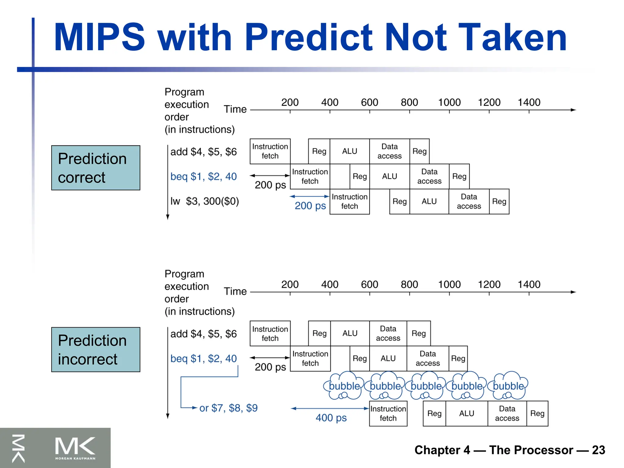
Chapter 4 —The Processor — 23
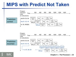
MIPS with Predict Not Taken
Prediction
correct
Prediction
incorrect
107.
Chapter 4 —The Processor — 24
More-Realistic Branch Prediction
Static branch prediction
Based on typical branch behavior
Example: loop and if-statement branches
Predict backward branches taken
Predict forward branches not taken
Dynamic branch prediction
Hardware measures actual branch behavior
e.g., record recent history of each branch
Assume future behavior will continue the trend
When wrong, stall while re-fetching, and update history
108.
Chapter 4 —The Processor — 25
Pipeline Summary
Pipelining improves performance by
increasing instruction throughput
Executes multiple instructions in parallel
Each instruction has the same latency
Subject to hazards
Structure, data, control
Instruction set design affects complexity of
pipeline implementation
The BIG Picture
109.
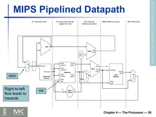
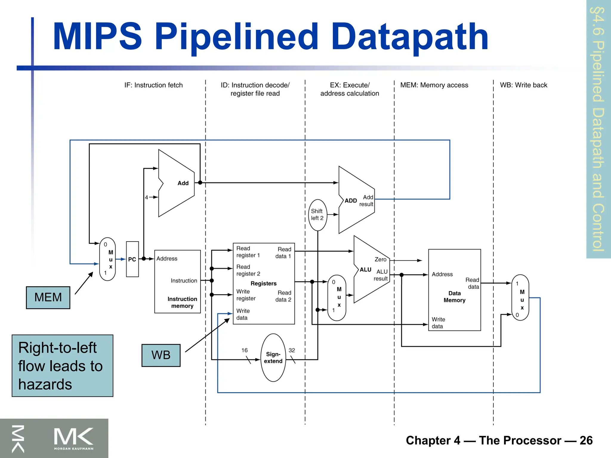
Chapter 4 —The Processor — 26
MIPS Pipelined Datapath
§4.6
Pipelined
Datapath
and
Control
WB
MEM
Right-to-left
flow leads to
hazards
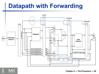
Chapter 4 —The Processor — 28
Datapath with Forwarding
112.
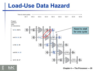
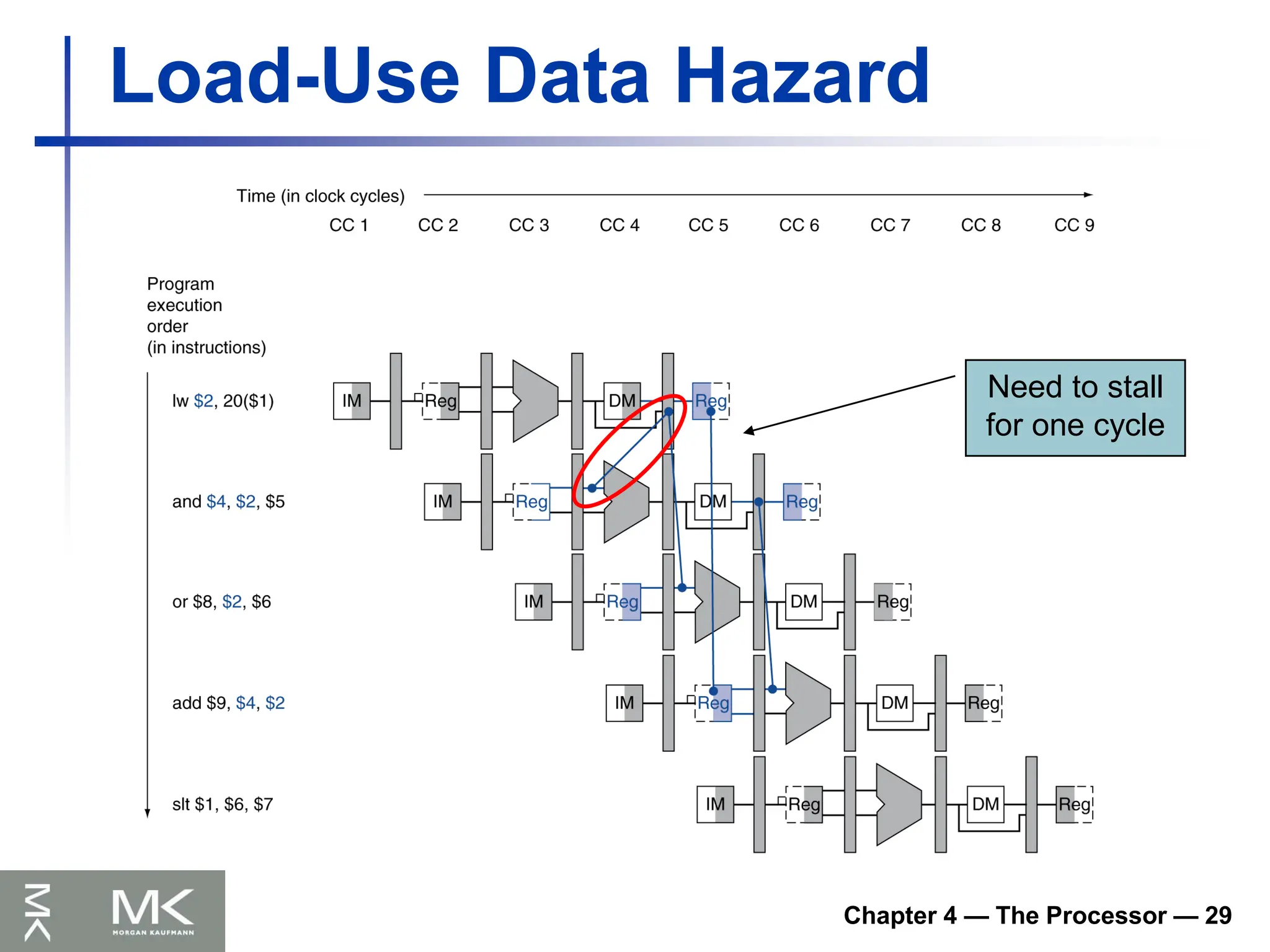
Chapter 4 —The Processor — 29
Load-Use Data Hazard
Need to stall
for one cycle
113.
Chapter 4 —The Processor — 30
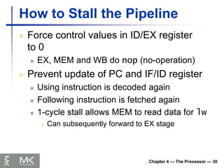
How to Stall the Pipeline
Force control values in ID/EX register
to 0
EX, MEM and WB do nop (no-operation)
Prevent update of PC and IF/ID register
Using instruction is decoded again
Following instruction is fetched again
1-cycle stall allows MEM to read data for lw
Can subsequently forward to EX stage
114.
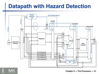
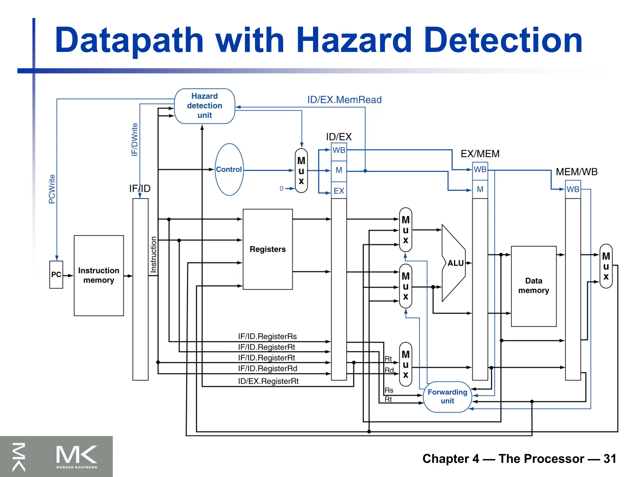
Chapter 4 —The Processor — 31
Datapath with Hazard Detection
115.
Chapter 4 —The Processor — 32
Stalls and Performance
Stalls reduce performance
But are required to get correct results
Compiler can arrange code to avoid
hazards and stalls
Requires knowledge of the pipeline structure
The BIG Picture
116.
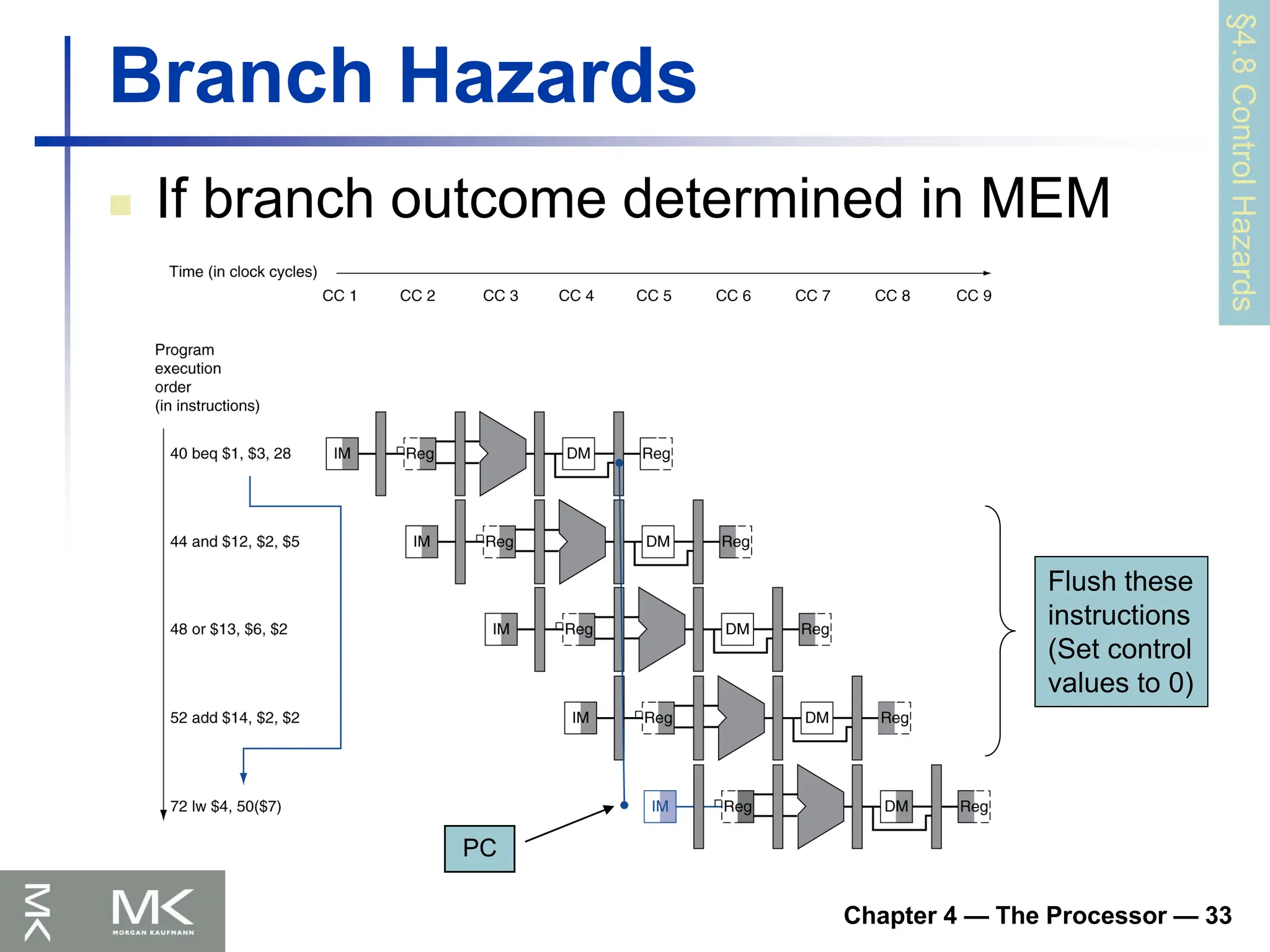
Chapter 4 —The Processor — 33
Branch Hazards
If branch outcome determined in MEM
§4.8
Control
Hazards
PC
Flush these
instructions
(Set control
values to 0)
117.
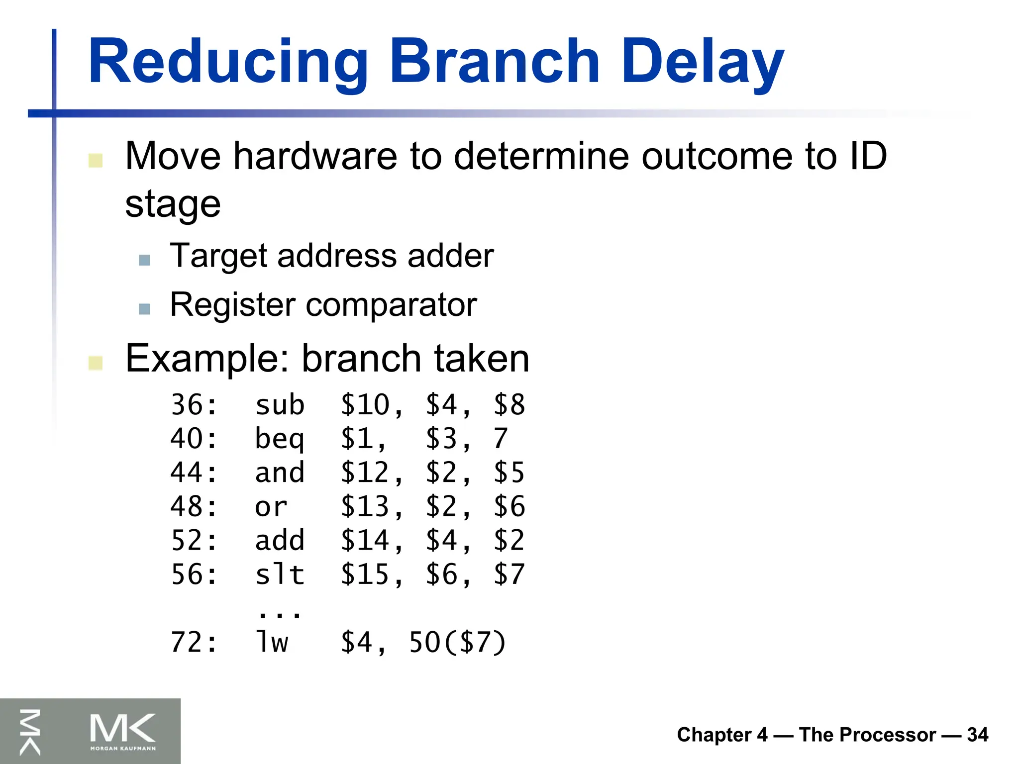
Chapter 4 —The Processor — 34
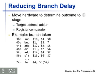
Reducing Branch Delay
Move hardware to determine outcome to ID
stage
Target address adder
Register comparator
Example: branch taken
36: sub $10, $4, $8
40: beq $1, $3, 7
44: and $12, $2, $5
48: or $13, $2, $6
52: add $14, $4, $2
56: slt $15, $6, $7
...
72: lw $4, 50($7)
118.
Chapter 4 —The Processor — 35
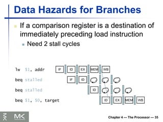
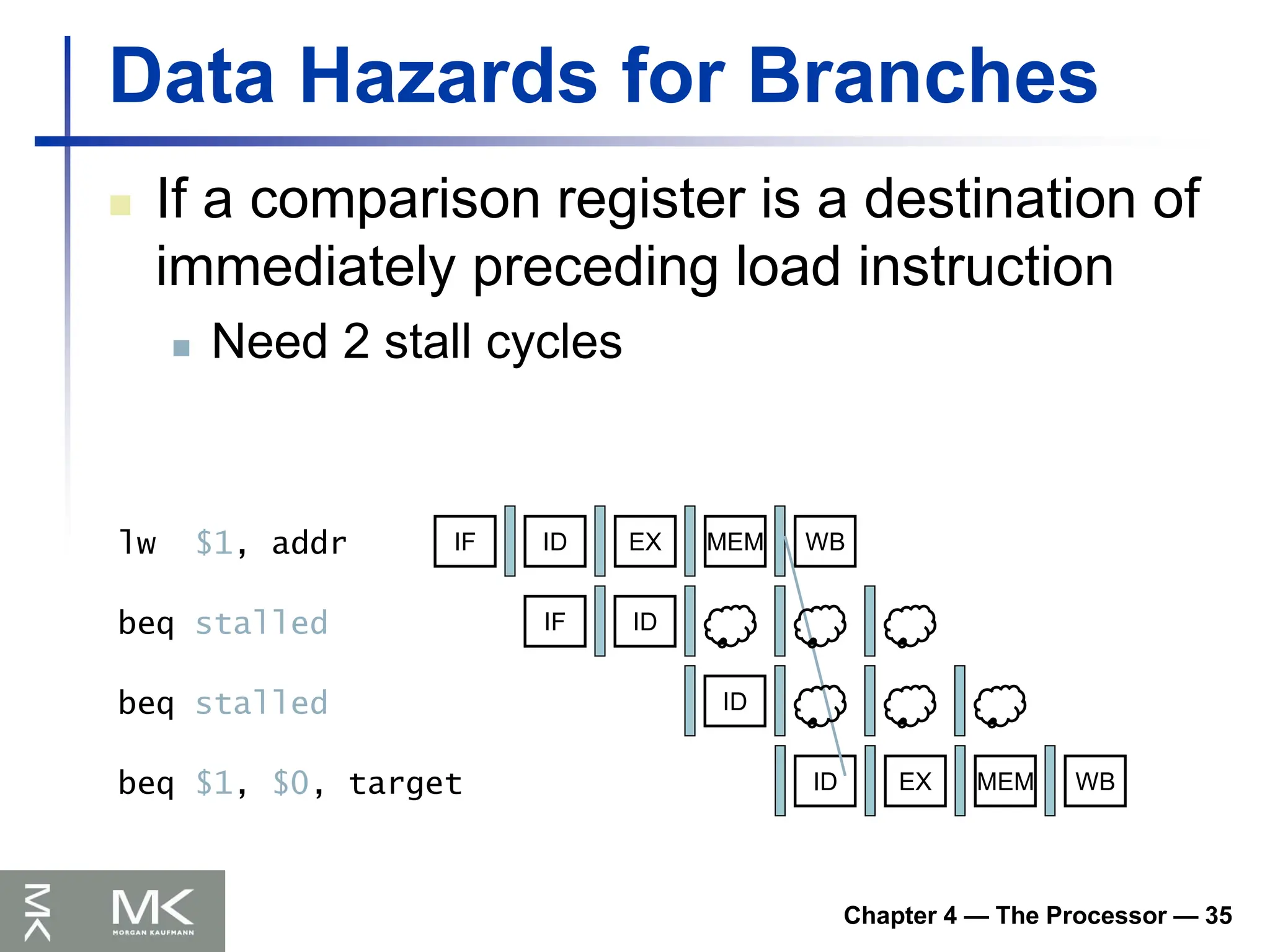
Data Hazards for Branches
If a comparison register is a destination of
immediately preceding load instruction
Need 2 stall cycles
beq stalled
IF ID EX MEM WB
IF ID
ID
ID EX MEM WB
beq stalled
lw $1, addr
beq $1, $0, target
119.
Chapter 4 —The Processor — 36
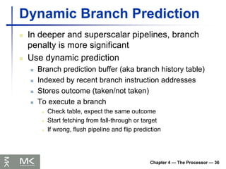
Dynamic Branch Prediction
In deeper and superscalar pipelines, branch
penalty is more significant
Use dynamic prediction
Branch prediction buffer (aka branch history table)
Indexed by recent branch instruction addresses
Stores outcome (taken/not taken)
To execute a branch
Check table, expect the same outcome
Start fetching from fall-through or target
If wrong, flush pipeline and flip prediction
120.
Chapter 4 —The Processor — 37
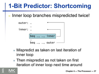
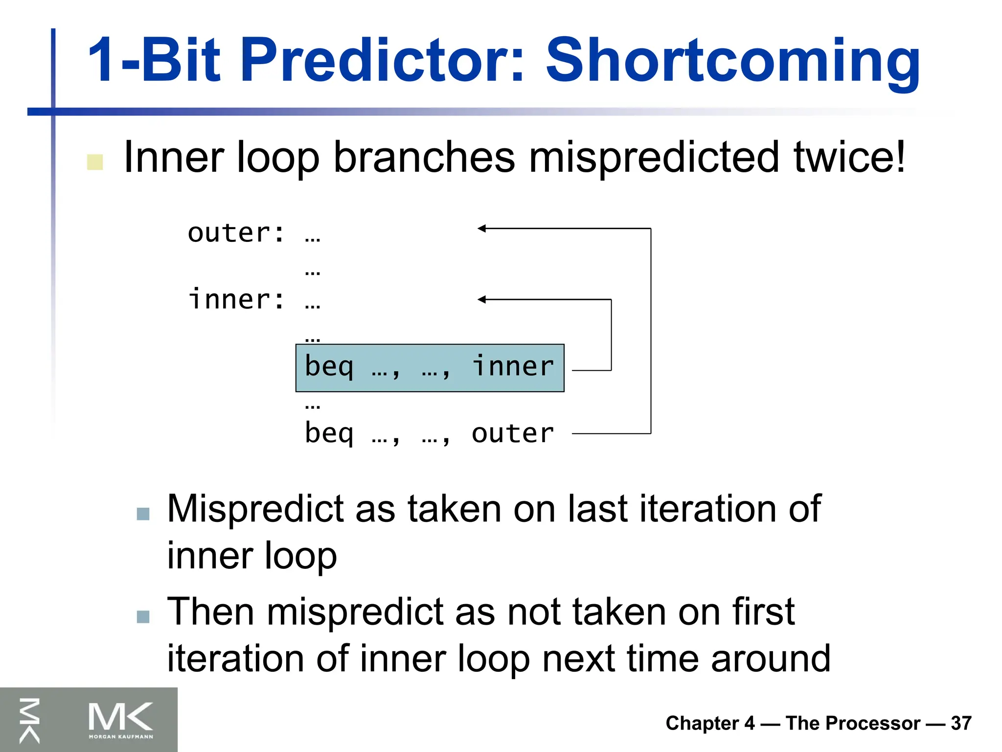
1-Bit Predictor: Shortcoming
Inner loop branches mispredicted twice!
outer: …
…
inner: …
…
beq …, …, inner
…
beq …, …, outer
Mispredict as taken on last iteration of
inner loop
Then mispredict as not taken on first
iteration of inner loop next time around
121.
Chapter 4 —The Processor — 38
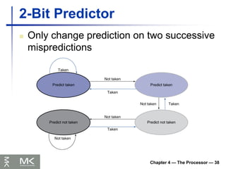
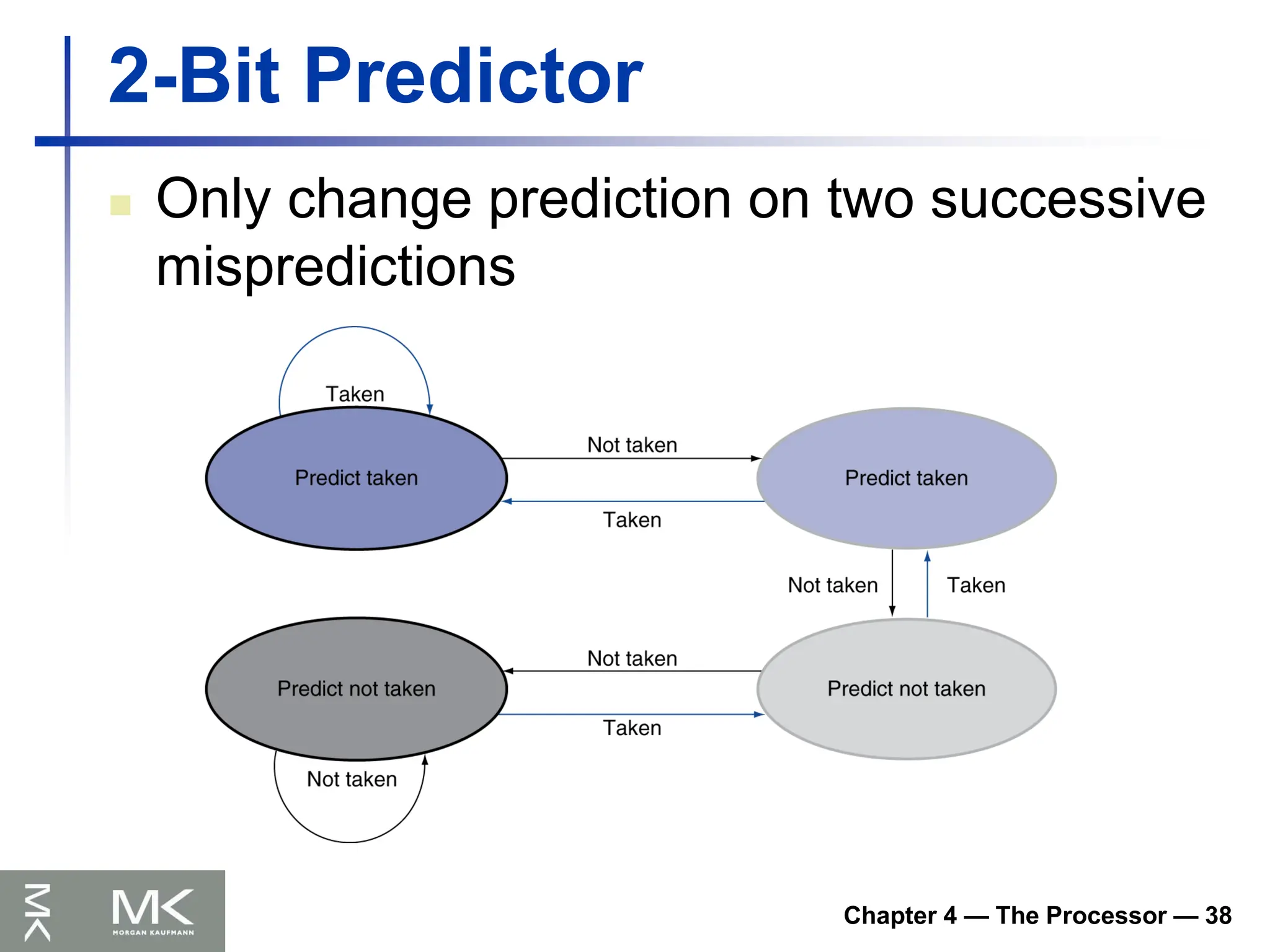
2-Bit Predictor
Only change prediction on two successive
mispredictions
122.
Chapter 4 —The Processor — 39
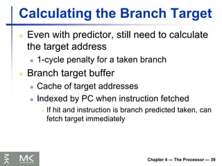
Calculating the Branch Target
Even with predictor, still need to calculate
the target address
1-cycle penalty for a taken branch
Branch target buffer
Cache of target addresses
Indexed by PC when instruction fetched
If hit and instruction is branch predicted taken, can
fetch target immediately
123.
Chapter 4 —The Processor — 40
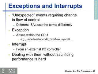
Exceptions and Interrupts
“Unexpected” events requiring change
in flow of control
Different ISAs use the terms differently
Exception
Arises within the CPU
e.g., undefined opcode, overflow, syscall, …
Interrupt
From an external I/O controller
Dealing with them without sacrificing
performance is hard
§4.9
Exceptions
124.
Chapter 4 —The Processor — 41
Handling Exceptions
In MIPS, exceptions managed by a System
Control Coprocessor (CP0)
Save PC of offending (or interrupted) instruction
In MIPS: Exception Program Counter (EPC)
Save indication of the problem
In MIPS: Cause register
We’ll assume 1-bit
0 for undefined opcode, 1 for overflow
Jump to handler at 8000 00180
125.
Chapter 4 —The Processor — 42
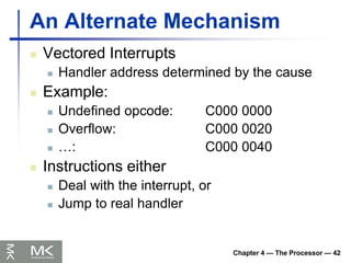
An Alternate Mechanism
Vectored Interrupts
Handler address determined by the cause
Example:
Undefined opcode: C000 0000
Overflow: C000 0020
…: C000 0040
Instructions either
Deal with the interrupt, or
Jump to real handler
126.
Chapter 4 —The Processor — 43
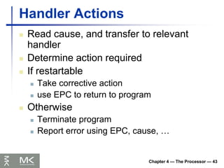
Handler Actions
Read cause, and transfer to relevant
handler
Determine action required
If restartable
Take corrective action
use EPC to return to program
Otherwise
Terminate program
Report error using EPC, cause, …
127.
Chapter 4 —The Processor — 44
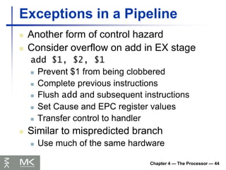
Exceptions in a Pipeline
Another form of control hazard
Consider overflow on add in EX stage
add $1, $2, $1
Prevent $1 from being clobbered
Complete previous instructions
Flush add and subsequent instructions
Set Cause and EPC register values
Transfer control to handler
Similar to mispredicted branch
Use much of the same hardware
128.
Chapter 4 —The Processor — 45
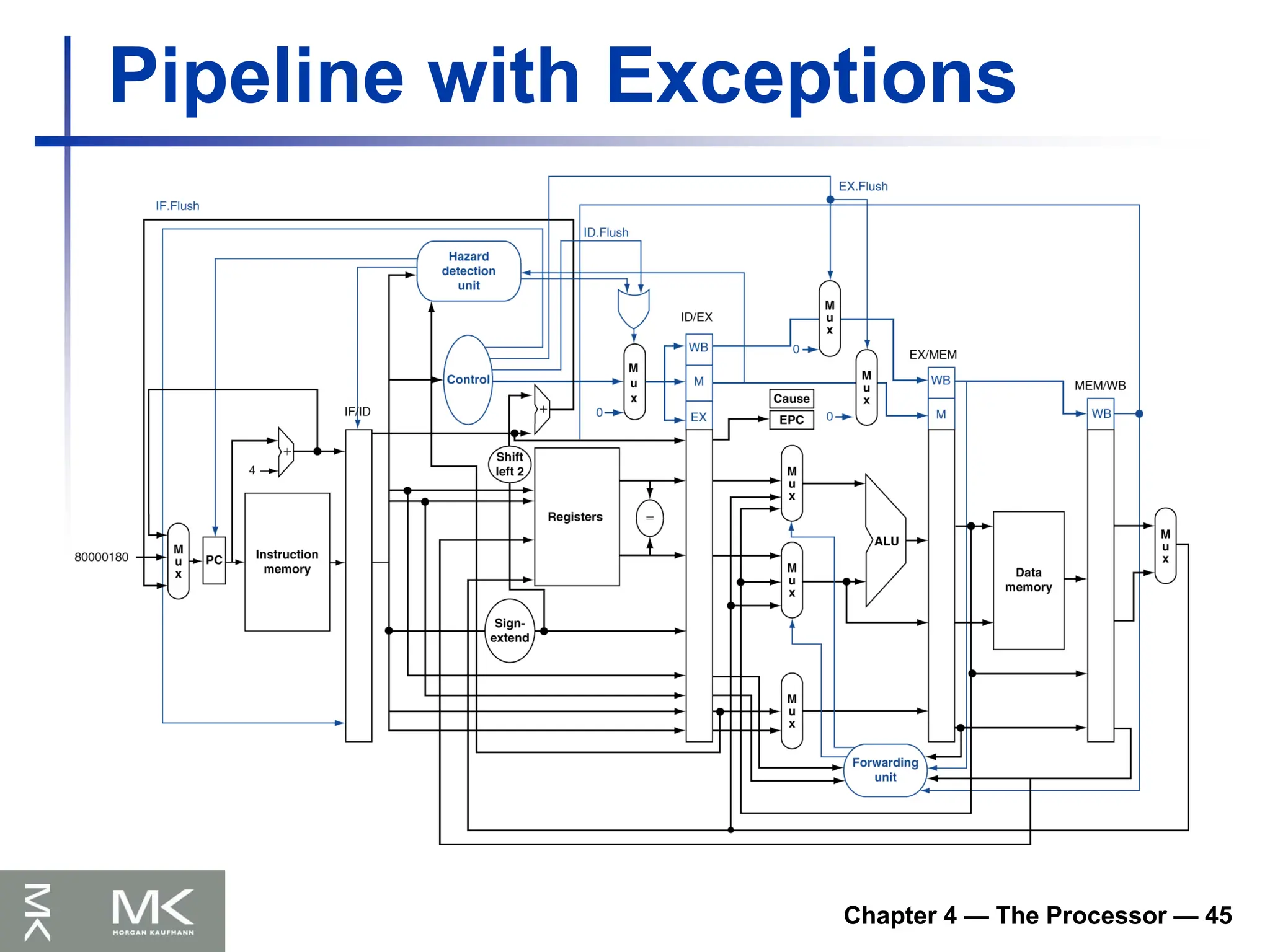
Pipeline with Exceptions
129.
Chapter 4 —The Processor — 46
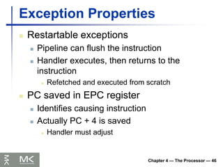
Exception Properties
Restartable exceptions
Pipeline can flush the instruction
Handler executes, then returns to the
instruction
Refetched and executed from scratch
PC saved in EPC register
Identifies causing instruction
Actually PC + 4 is saved
Handler must adjust
130.
Chapter 4 —The Processor — 47
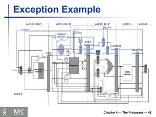
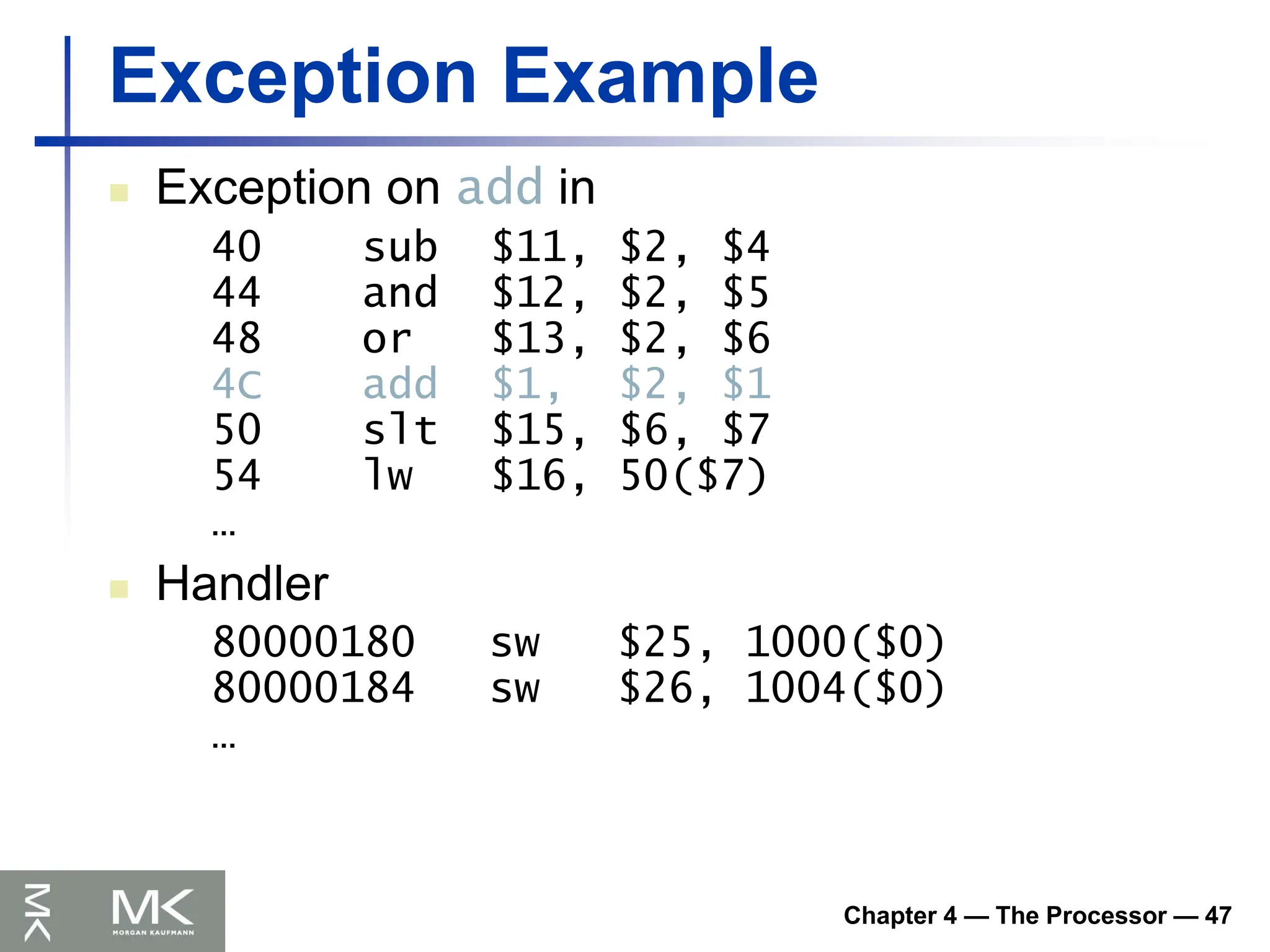
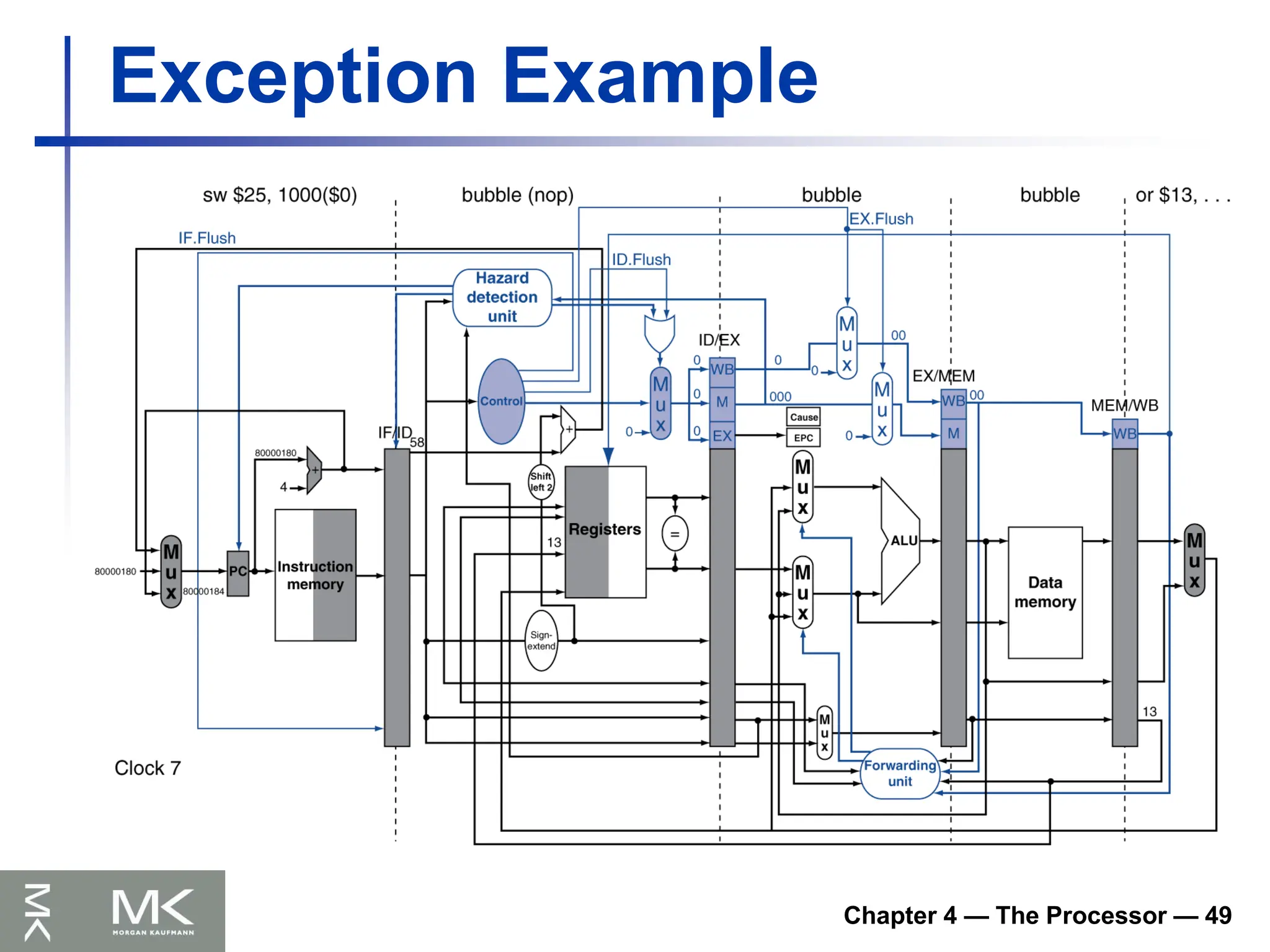
Exception Example
Exception on add in
40 sub $11, $2, $4
44 and $12, $2, $5
48 or $13, $2, $6
4C add $1, $2, $1
50 slt $15, $6, $7
54 lw $16, 50($7)
…
Handler
80000180 sw $25, 1000($0)
80000184 sw $26, 1004($0)
…
Chapter 4 —The Processor — 50
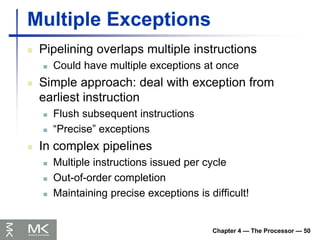
Multiple Exceptions
Pipelining overlaps multiple instructions
Could have multiple exceptions at once
Simple approach: deal with exception from
earliest instruction
Flush subsequent instructions
“Precise” exceptions
In complex pipelines
Multiple instructions issued per cycle
Out-of-order completion
Maintaining precise exceptions is difficult!
134.
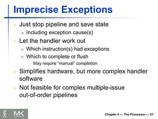
Chapter 4 —The Processor — 51
Imprecise Exceptions
Just stop pipeline and save state
Including exception cause(s)
Let the handler work out
Which instruction(s) had exceptions
Which to complete or flush
May require “manual” completion
Simplifies hardware, but more complex handler
software
Not feasible for complex multiple-issue
out-of-order pipelines
135.
Chapter 4 —The Processor — 52
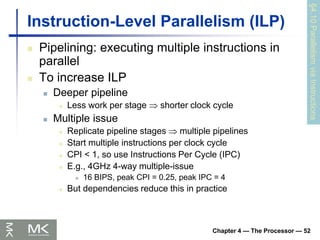
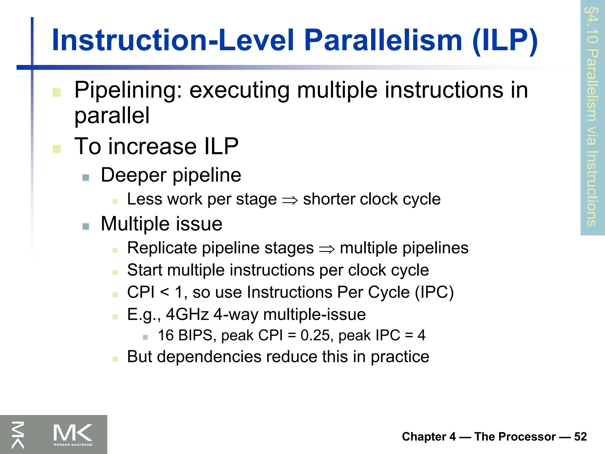
Instruction-Level Parallelism (ILP)
Pipelining: executing multiple instructions in
parallel
To increase ILP
Deeper pipeline
Less work per stage shorter clock cycle
Multiple issue
Replicate pipeline stages multiple pipelines
Start multiple instructions per clock cycle
CPI < 1, so use Instructions Per Cycle (IPC)
E.g., 4GHz 4-way multiple-issue
16 BIPS, peak CPI = 0.25, peak IPC = 4
But dependencies reduce this in practice
§4.10
Parallelism
via
Instructions
136.
COMPUTER ORGANIZATION ANDDESIGN
The Hardware/Software Interface
5th
Edition
Chapter 5
Large and Fast:
Exploiting Memory
Hierarchy
137.
Chapter 5 —Large and Fast: Exploiting Memory Hierarchy — 2
Principle of Locality
Programs access a small proportion of
their address space at any time
Temporal locality
Items accessed recently are likely to be
accessed again soon
e.g., instructions in a loop, induction variables
Spatial locality
Items near those accessed recently are likely
to be accessed soon
E.g., sequential instruction access, array data
§5.1
Introduction
138.
Chapter 5 —Large and Fast: Exploiting Memory Hierarchy — 3
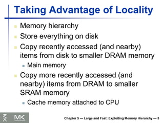
Taking Advantage of Locality
Memory hierarchy
Store everything on disk
Copy recently accessed (and nearby)
items from disk to smaller DRAM memory
Main memory
Copy more recently accessed (and
nearby) items from DRAM to smaller
SRAM memory
Cache memory attached to CPU
139.
Chapter 5 —Large and Fast: Exploiting Memory Hierarchy — 4
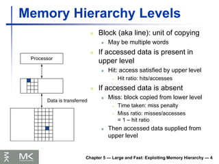
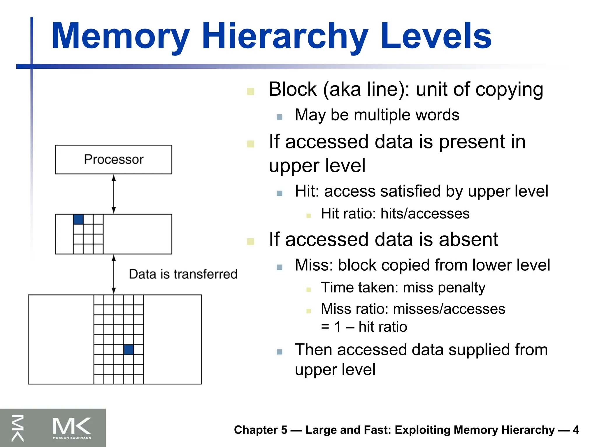
Memory Hierarchy Levels
Block (aka line): unit of copying
May be multiple words
If accessed data is present in
upper level
Hit: access satisfied by upper level
Hit ratio: hits/accesses
If accessed data is absent
Miss: block copied from lower level
Time taken: miss penalty
Miss ratio: misses/accesses
= 1 – hit ratio
Then accessed data supplied from
upper level
140.
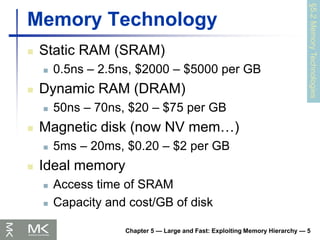
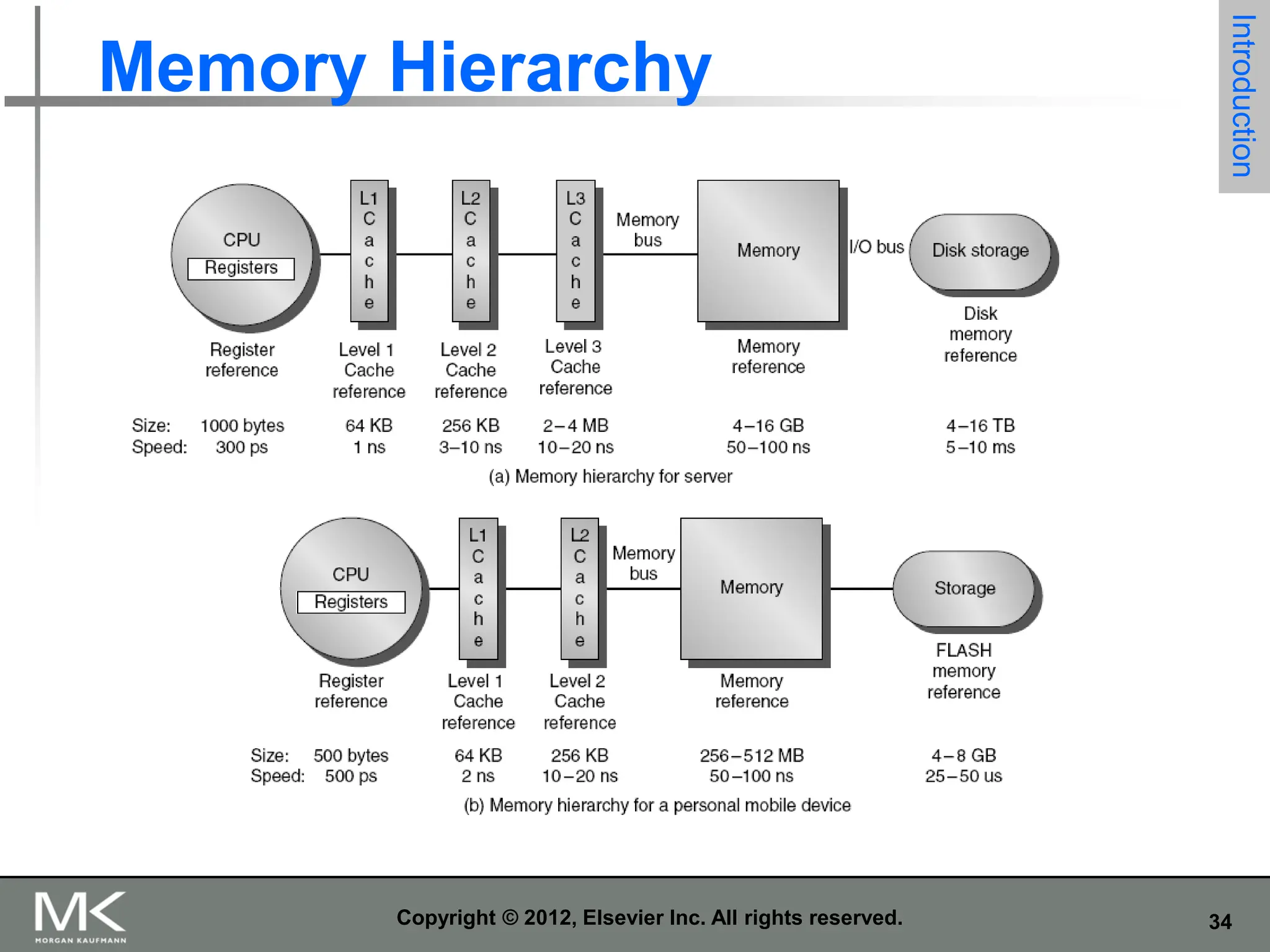
Chapter 5 —Large and Fast: Exploiting Memory Hierarchy — 5
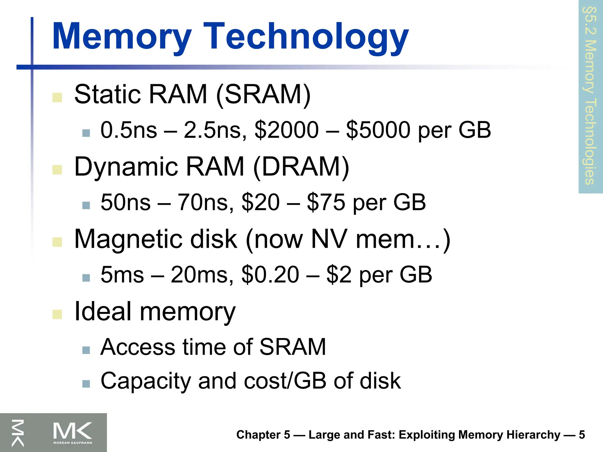
Memory Technology
Static RAM (SRAM)
0.5ns – 2.5ns, $2000 – $5000 per GB
Dynamic RAM (DRAM)
50ns – 70ns, $20 – $75 per GB
Magnetic disk (now NV mem…)
5ms – 20ms, $0.20 – $2 per GB
Ideal memory
Access time of SRAM
Capacity and cost/GB of disk
§5.2
Memory
Technologies
141.
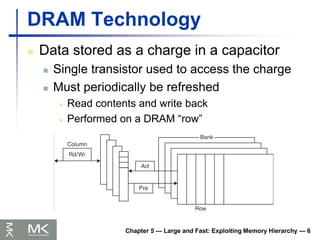
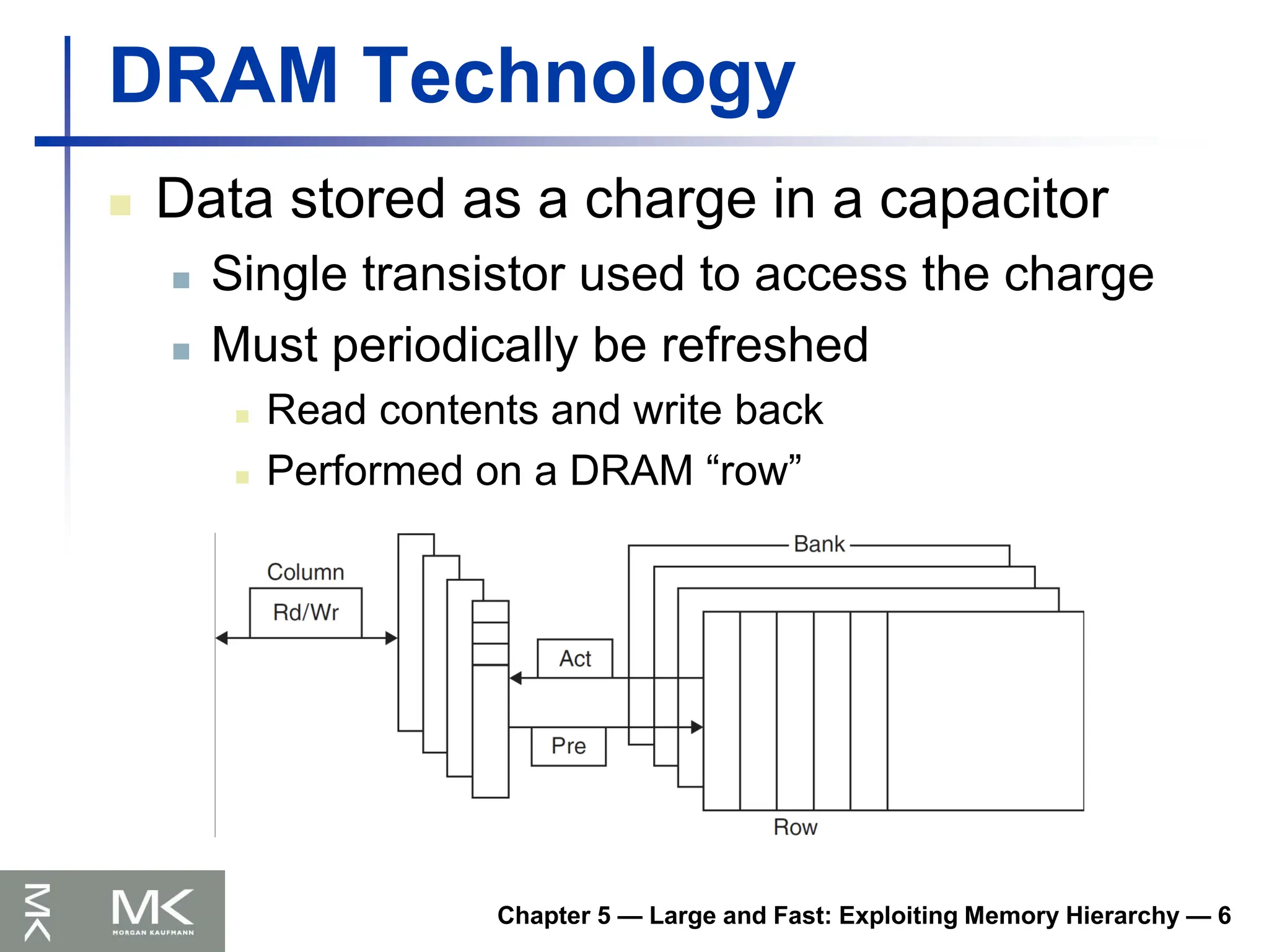
DRAM Technology
Datastored as a charge in a capacitor
Single transistor used to access the charge
Must periodically be refreshed
Read contents and write back
Performed on a DRAM “row”
Chapter 5 — Large and Fast: Exploiting Memory Hierarchy — 6
142.
Chapter 5 —Large and Fast: Exploiting Memory Hierarchy — 7
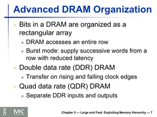
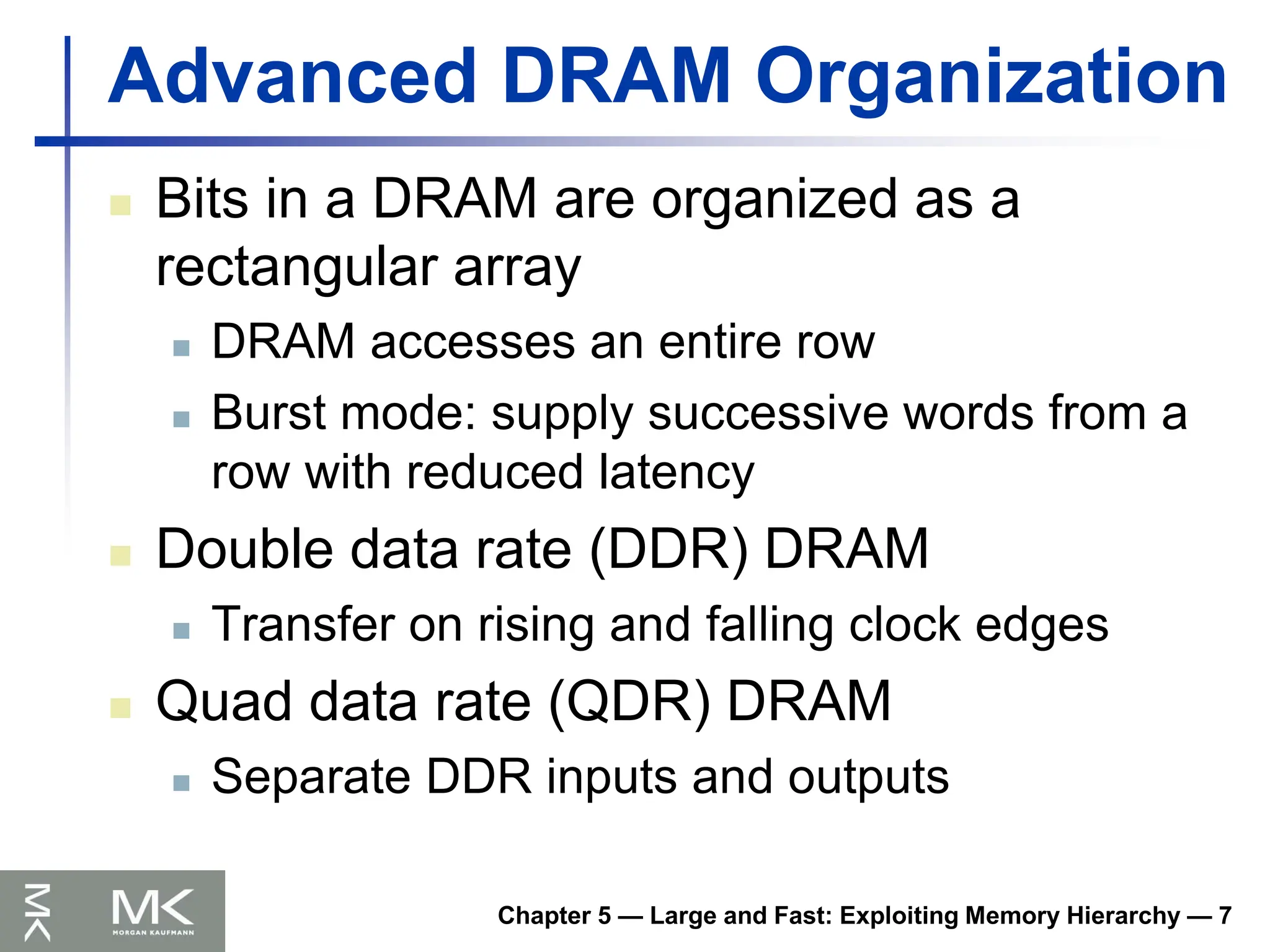
Advanced DRAM Organization
Bits in a DRAM are organized as a
rectangular array
DRAM accesses an entire row
Burst mode: supply successive words from a
row with reduced latency
Double data rate (DDR) DRAM
Transfer on rising and falling clock edges
Quad data rate (QDR) DRAM
Separate DDR inputs and outputs
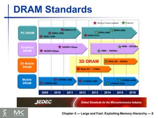
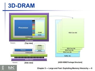
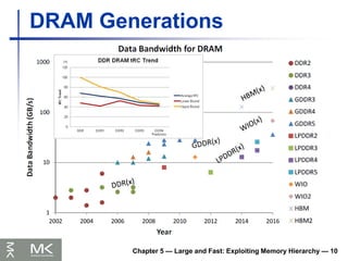
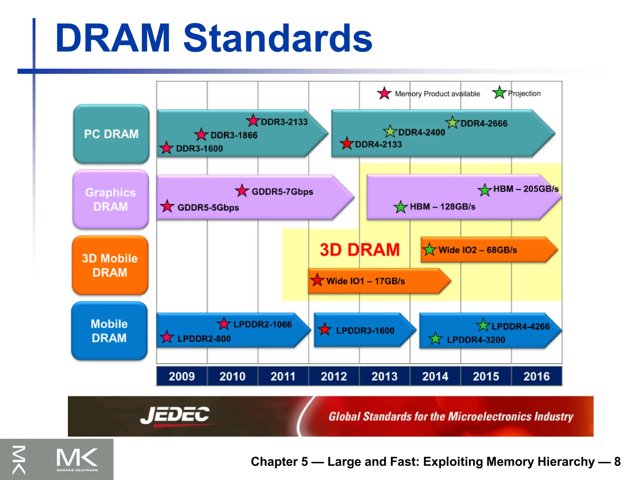
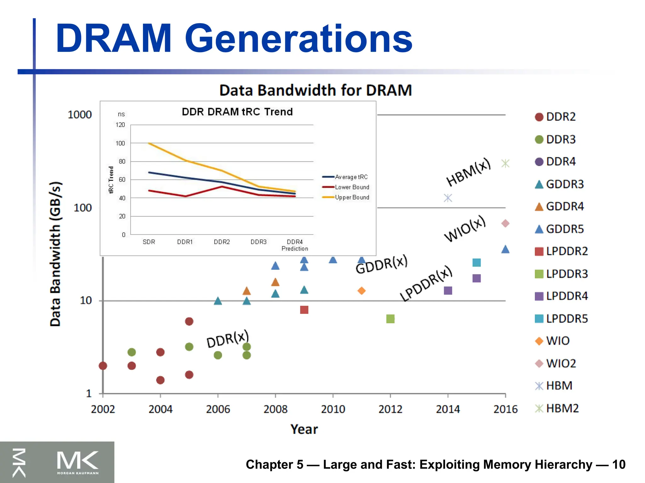
Chapter 5 —Large and Fast: Exploiting Memory Hierarchy — 10
DRAM Generations
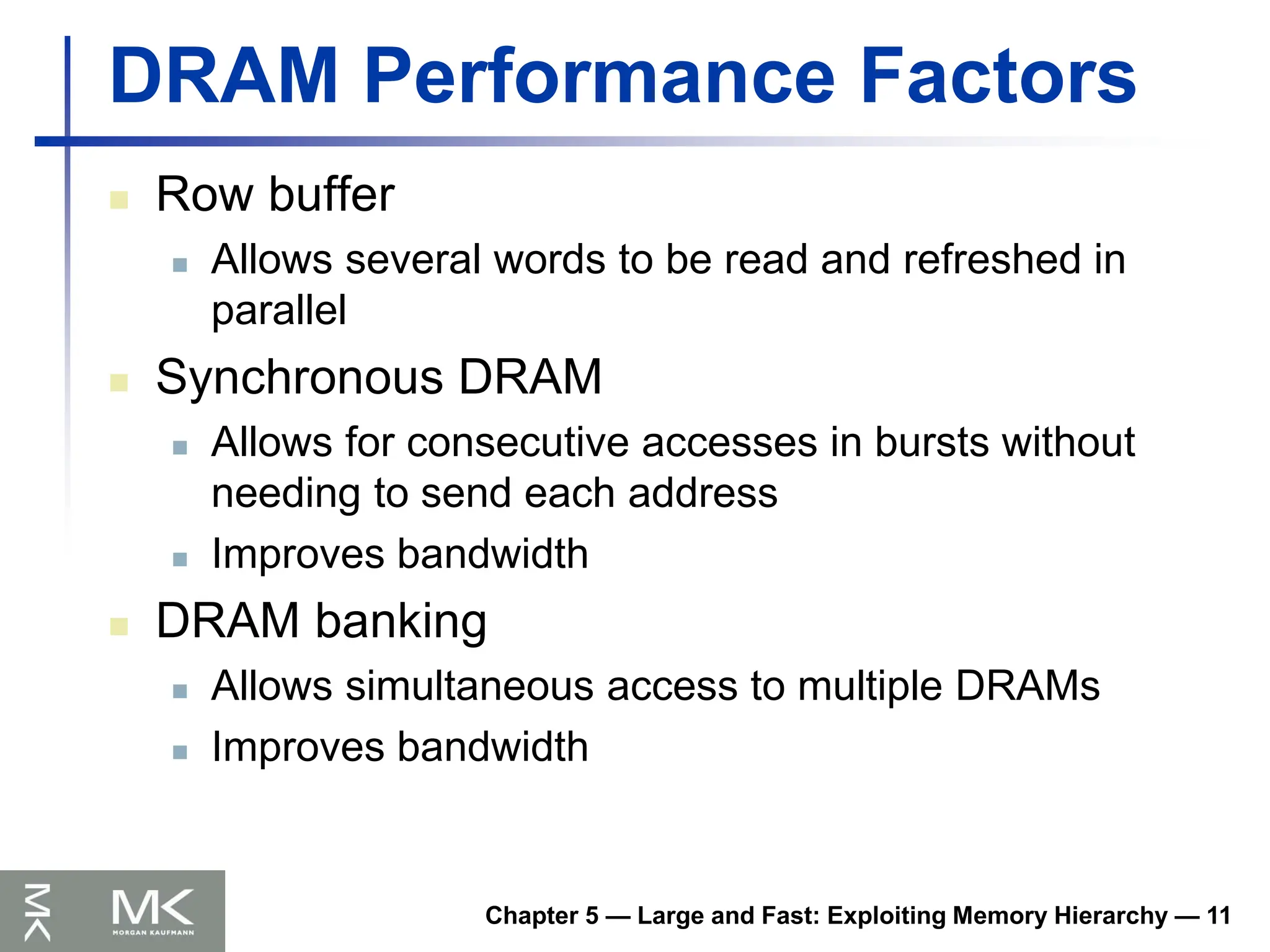
146.
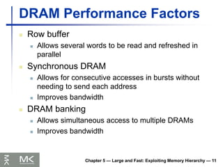
DRAM Performance Factors
Row buffer
Allows several words to be read and refreshed in
parallel
Synchronous DRAM
Allows for consecutive accesses in bursts without
needing to send each address
Improves bandwidth
DRAM banking
Allows simultaneous access to multiple DRAMs
Improves bandwidth
Chapter 5 — Large and Fast: Exploiting Memory Hierarchy — 11
Chapter 5 —Large and Fast: Exploiting Memory Hierarchy — 13
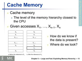
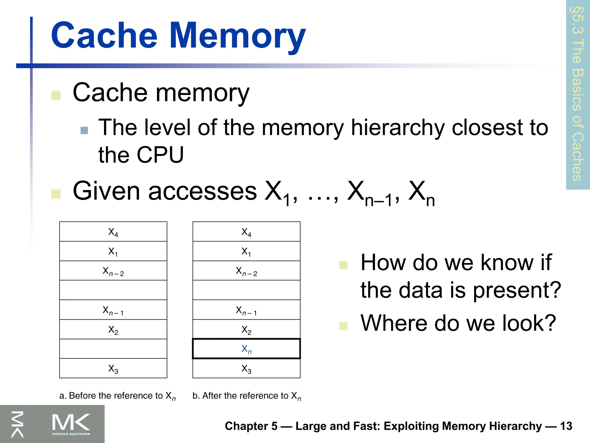
Cache Memory
Cache memory
The level of the memory hierarchy closest to
the CPU
Given accesses X1, …, Xn–1, Xn
§5.3
The
Basics
of
Caches
How do we know if
the data is present?
Where do we look?
149.
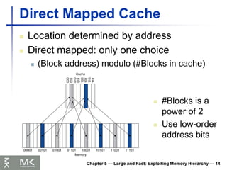
Chapter 5 —Large and Fast: Exploiting Memory Hierarchy — 14
Direct Mapped Cache
Location determined by address
Direct mapped: only one choice
(Block address) modulo (#Blocks in cache)
#Blocks is a
power of 2
Use low-order
address bits
150.
Chapter 5 —Large and Fast: Exploiting Memory Hierarchy — 15
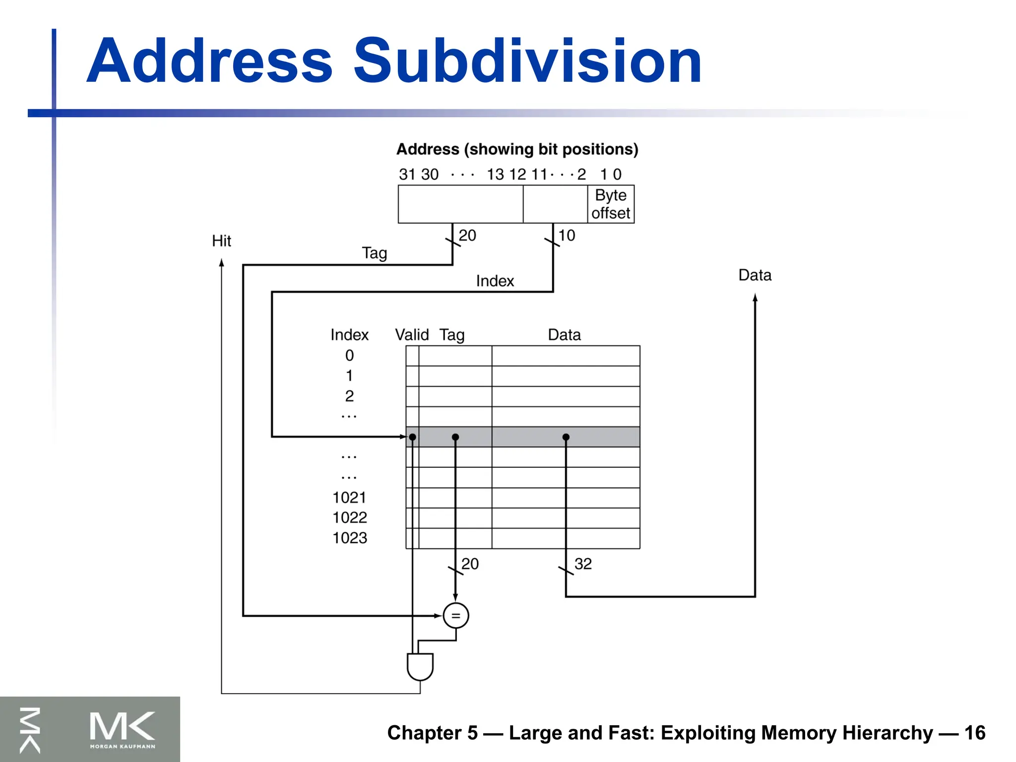
Tags and Valid Bits
How do we know which particular block is
stored in a cache location?
Store block address as well as the data
Actually, only need the high-order bits
Called the tag
What if there is no data in a location?
Valid bit: 1 = present, 0 = not present
Initially 0
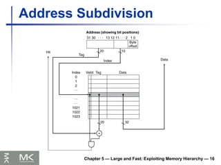
Chapter 5 —Large and Fast: Exploiting Memory Hierarchy — 17
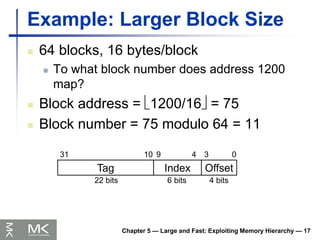
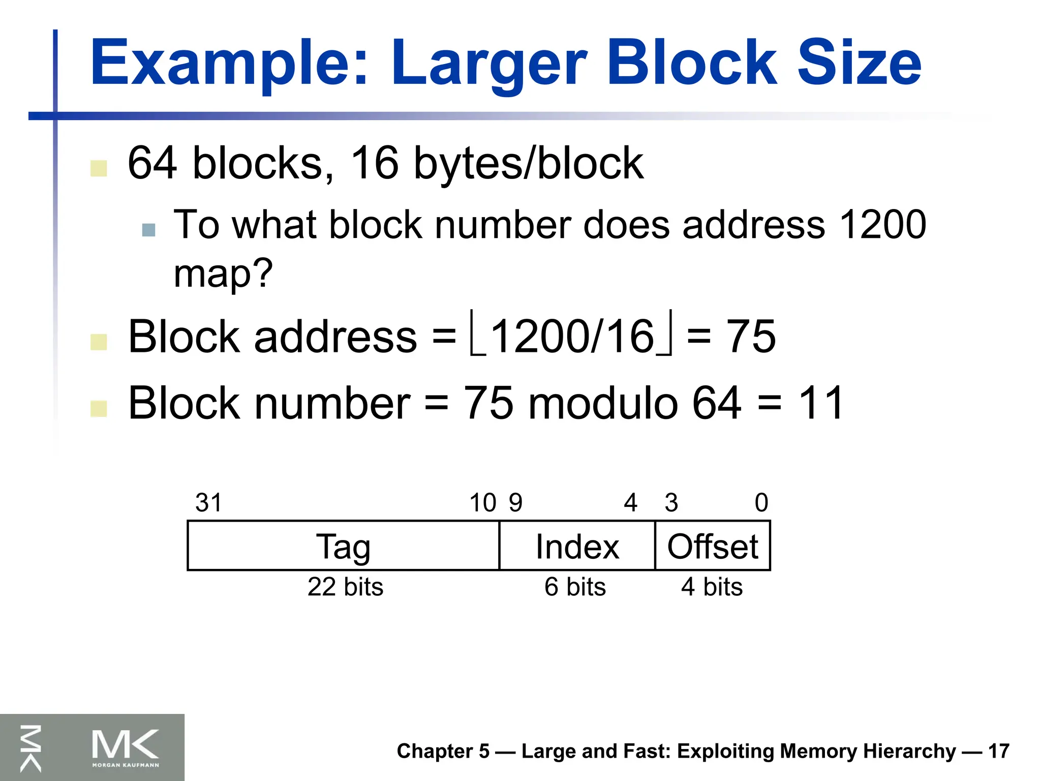
Example: Larger Block Size
64 blocks, 16 bytes/block
To what block number does address 1200
map?
Block address = 1200/16 = 75
Block number = 75 modulo 64 = 11
Tag Index Offset
0
3
4
9
10
31
4 bits
6 bits
22 bits
153.
Chapter 5 —Large and Fast: Exploiting Memory Hierarchy — 18
Block Size Considerations
Larger blocks should reduce miss rate
Due to spatial locality
But in a fixed-sized cache
Larger blocks fewer of them
More competition increased miss rate
Larger blocks pollution
Larger miss penalty
Can override benefit of reduced miss rate
Early restart and critical-word-first can help
154.
Chapter 5 —Large and Fast: Exploiting Memory Hierarchy — 19
Cache Misses
On cache hit, CPU proceeds normally
On cache miss
Stall the CPU pipeline
Fetch block from next level of hierarchy
Instruction cache miss
Restart instruction fetch
Data cache miss
Complete data access
155.
Chapter 5 —Large and Fast: Exploiting Memory Hierarchy — 20
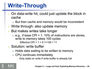
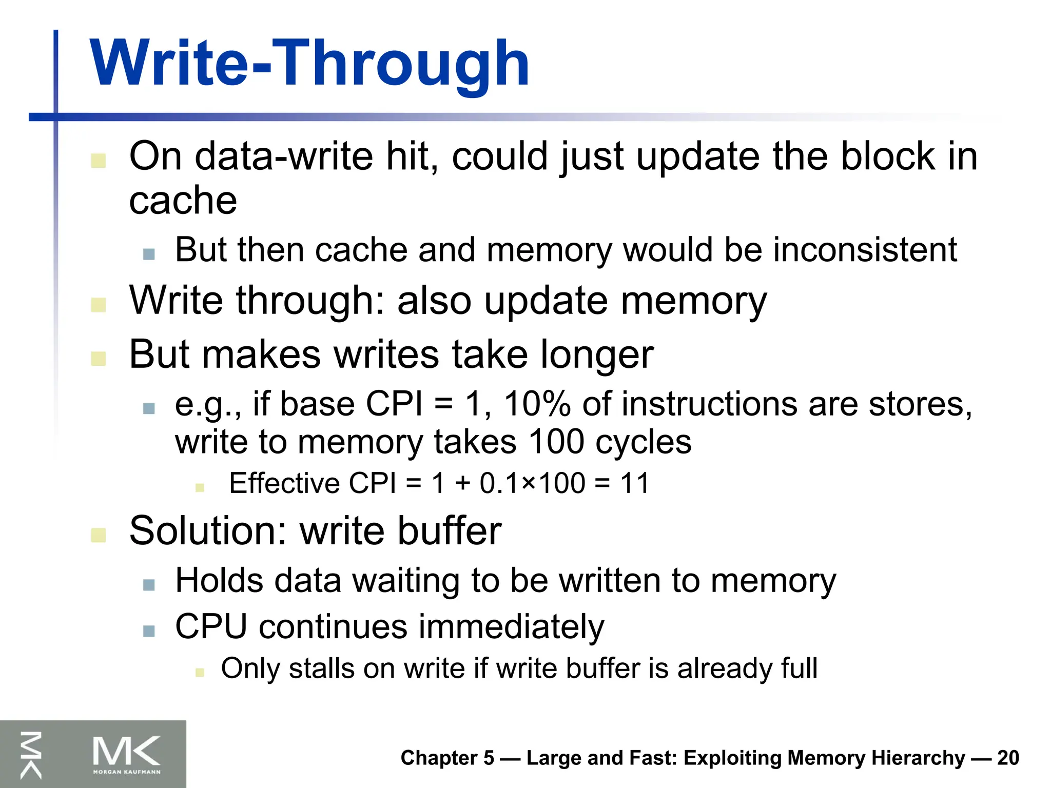
Write-Through
On data-write hit, could just update the block in
cache
But then cache and memory would be inconsistent
Write through: also update memory
But makes writes take longer
e.g., if base CPI = 1, 10% of instructions are stores,
write to memory takes 100 cycles
Effective CPI = 1 + 0.1×100 = 11
Solution: write buffer
Holds data waiting to be written to memory
CPU continues immediately
Only stalls on write if write buffer is already full
156.
Chapter 5 —Large and Fast: Exploiting Memory Hierarchy — 21
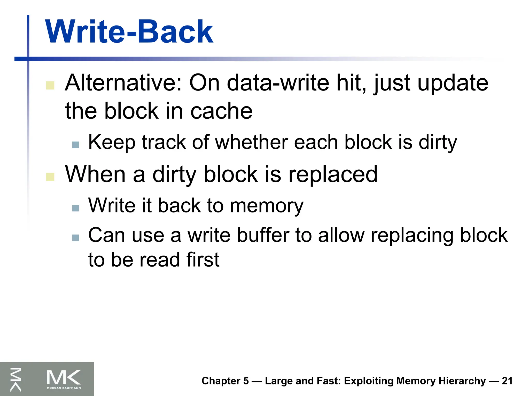
Write-Back
Alternative: On data-write hit, just update
the block in cache
Keep track of whether each block is dirty
When a dirty block is replaced
Write it back to memory
Can use a write buffer to allow replacing block
to be read first
157.
Chapter 5 —Large and Fast: Exploiting Memory Hierarchy — 22
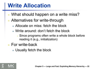
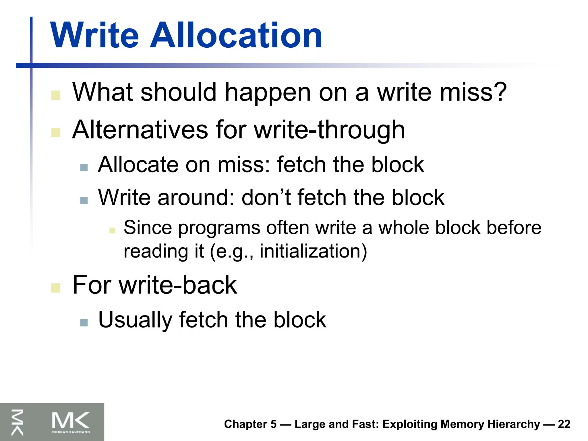
Write Allocation
What should happen on a write miss?
Alternatives for write-through
Allocate on miss: fetch the block
Write around: don’t fetch the block
Since programs often write a whole block before
reading it (e.g., initialization)
For write-back
Usually fetch the block
158.
Chapter 5 —Large and Fast: Exploiting Memory Hierarchy — 23
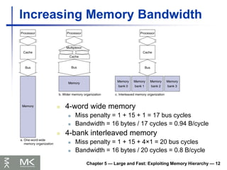
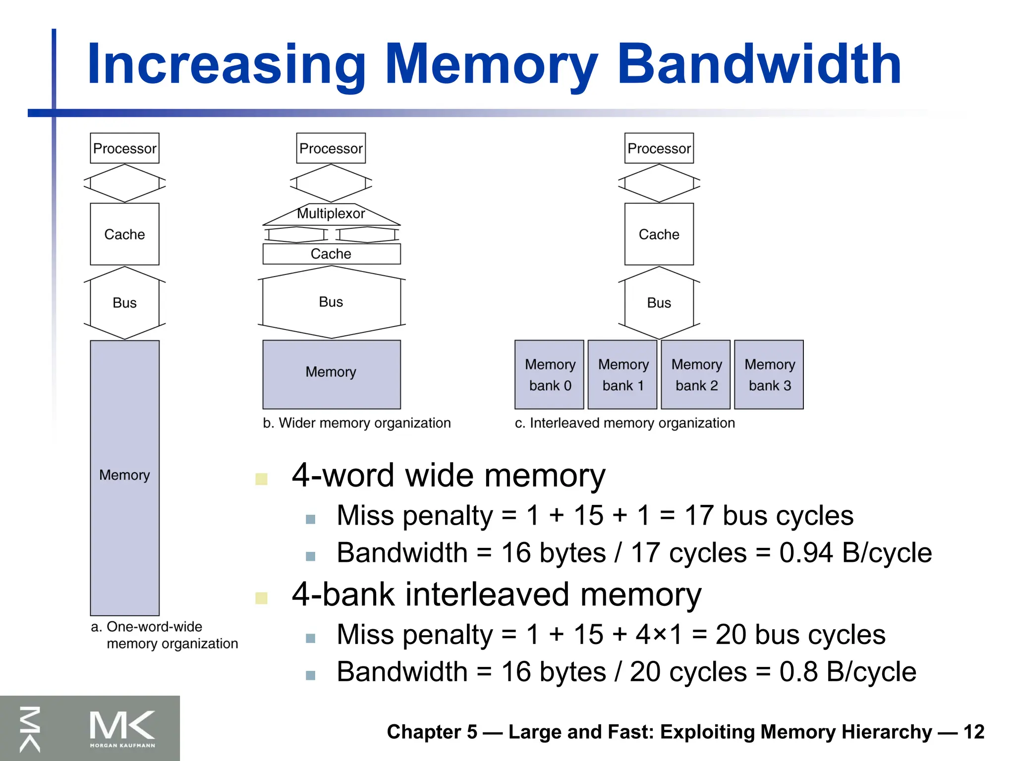
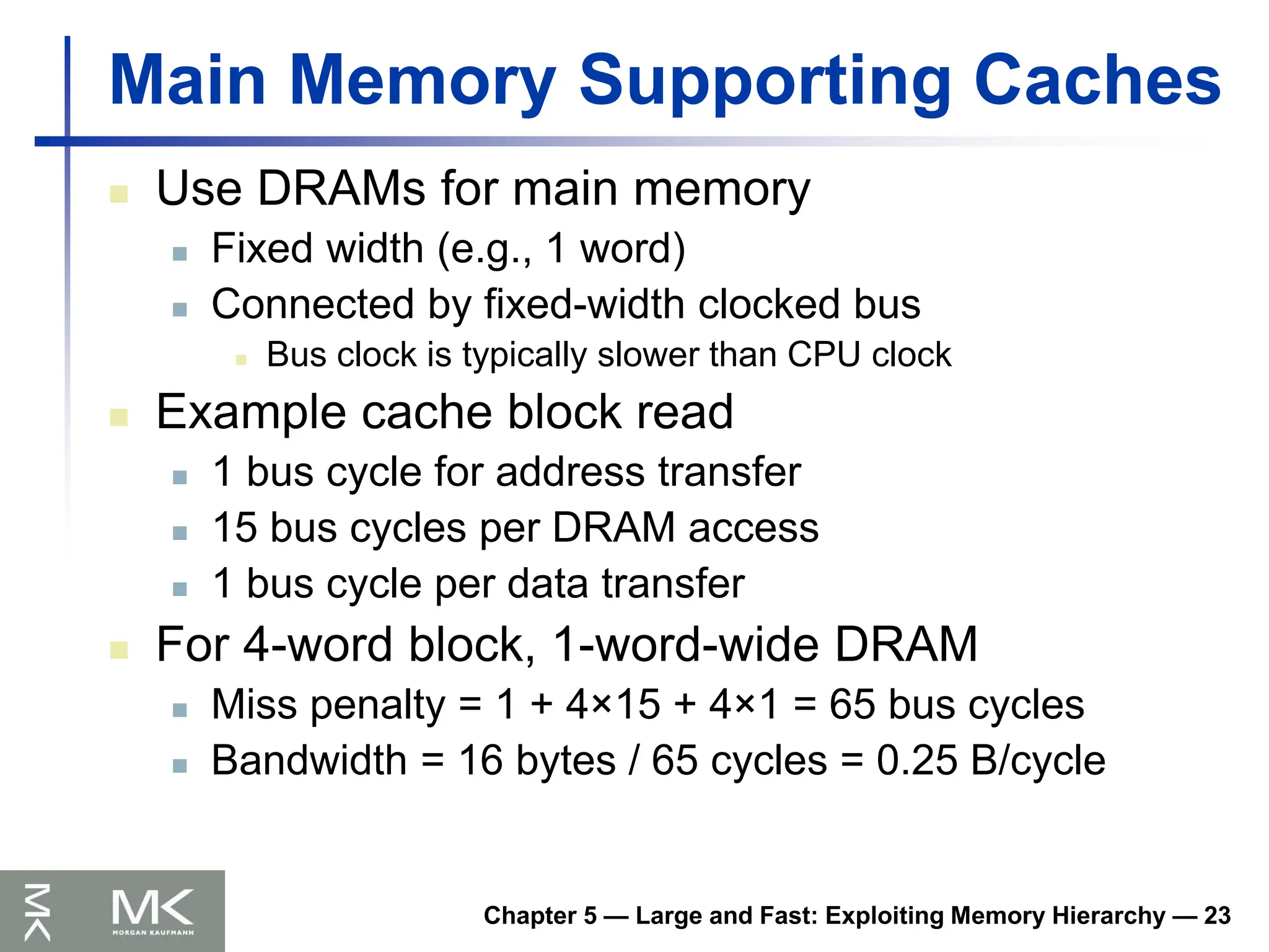
Main Memory Supporting Caches
Use DRAMs for main memory
Fixed width (e.g., 1 word)
Connected by fixed-width clocked bus
Bus clock is typically slower than CPU clock
Example cache block read
1 bus cycle for address transfer
15 bus cycles per DRAM access
1 bus cycle per data transfer
For 4-word block, 1-word-wide DRAM
Miss penalty = 1 + 4×15 + 4×1 = 65 bus cycles
Bandwidth = 16 bytes / 65 cycles = 0.25 B/cycle
159.
Chapter 5 —Large and Fast: Exploiting Memory Hierarchy — 24
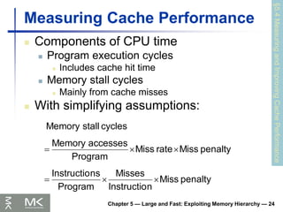
Measuring Cache Performance
Components of CPU time
Program execution cycles
Includes cache hit time
Memory stall cycles
Mainly from cache misses
With simplifying assumptions:
§5.4
Measuring
and
Improving
Cache
Performance
penalty
Miss
n
Instructio
Misses
Program
ns
Instructio
penalty
Miss
rate
Miss
Program
accesses
Memory
cycles
stall
Memory
160.
Chapter 5 —Large and Fast: Exploiting Memory Hierarchy — 25
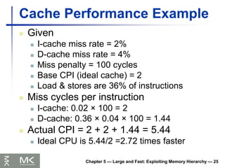
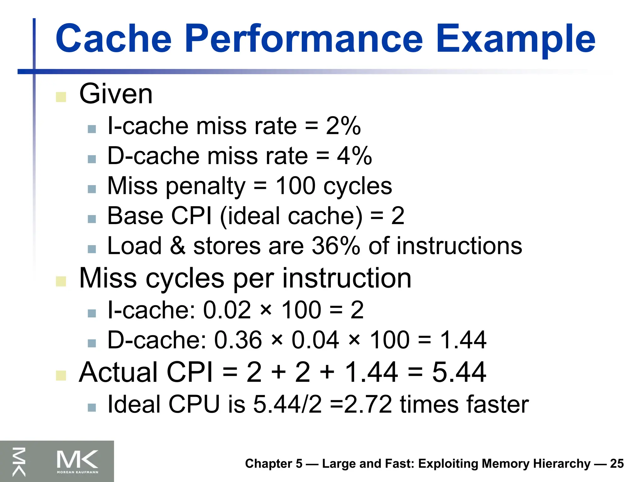
Cache Performance Example
Given
I-cache miss rate = 2%
D-cache miss rate = 4%
Miss penalty = 100 cycles
Base CPI (ideal cache) = 2
Load & stores are 36% of instructions
Miss cycles per instruction
I-cache: 0.02 × 100 = 2
D-cache: 0.36 × 0.04 × 100 = 1.44
Actual CPI = 2 + 2 + 1.44 = 5.44
Ideal CPU is 5.44/2 =2.72 times faster
161.
Chapter 5 —Large and Fast: Exploiting Memory Hierarchy — 26
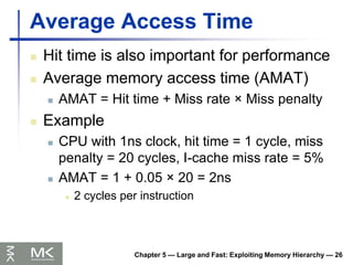
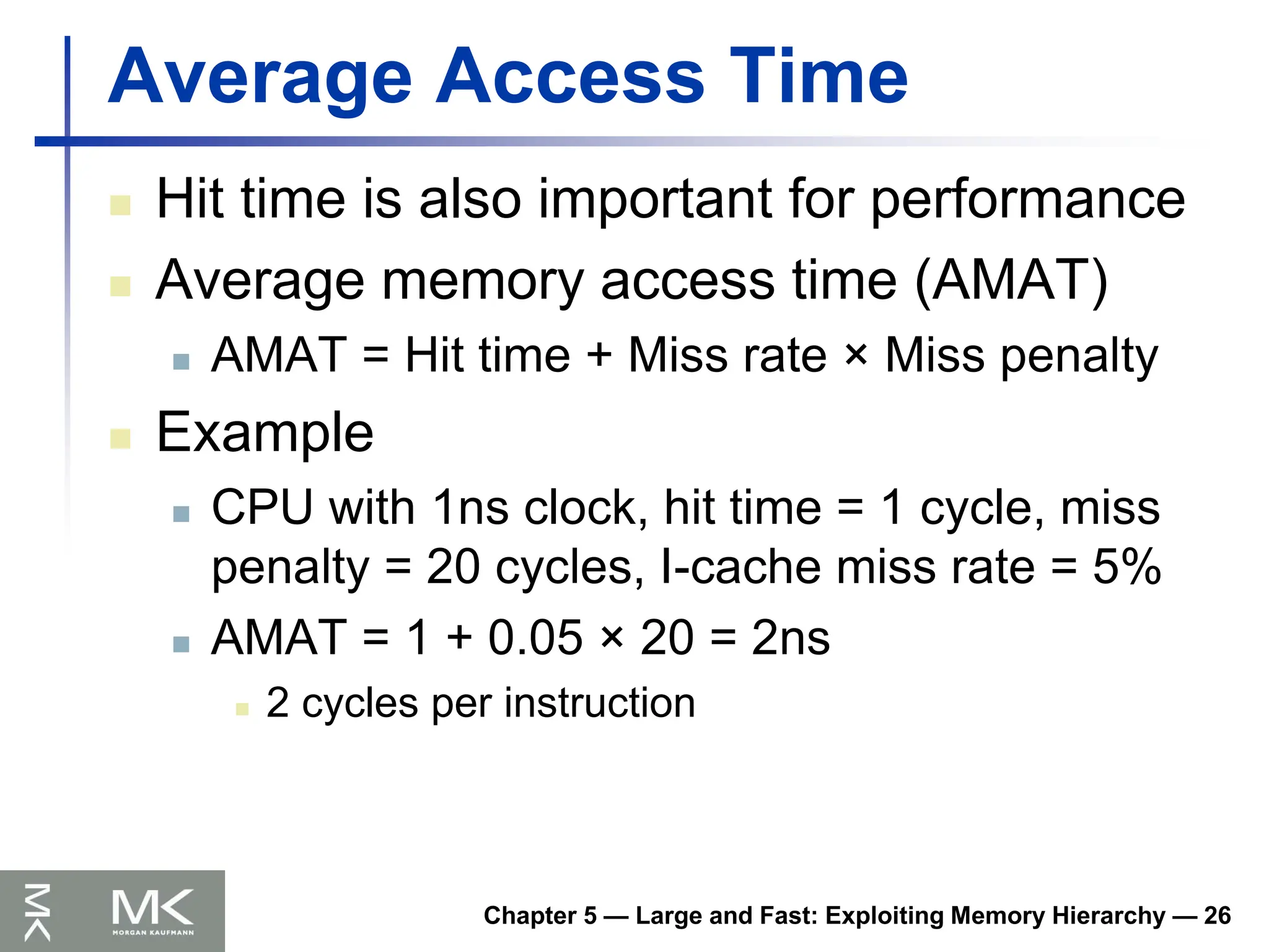
Average Access Time
Hit time is also important for performance
Average memory access time (AMAT)
AMAT = Hit time + Miss rate × Miss penalty
Example
CPU with 1ns clock, hit time = 1 cycle, miss
penalty = 20 cycles, I-cache miss rate = 5%
AMAT = 1 + 0.05 × 20 = 2ns
2 cycles per instruction
162.
Chapter 5 —Large and Fast: Exploiting Memory Hierarchy — 27
Performance Summary
When CPU performance increased
Miss penalty becomes more significant
Decreasing base CPI
Greater proportion of time spent on memory
stalls
Increasing clock rate
Memory stalls account for more CPU cycles
Can’t neglect cache behavior when
evaluating system performance
163.
Chapter 5 —Large and Fast: Exploiting Memory Hierarchy — 28
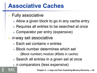
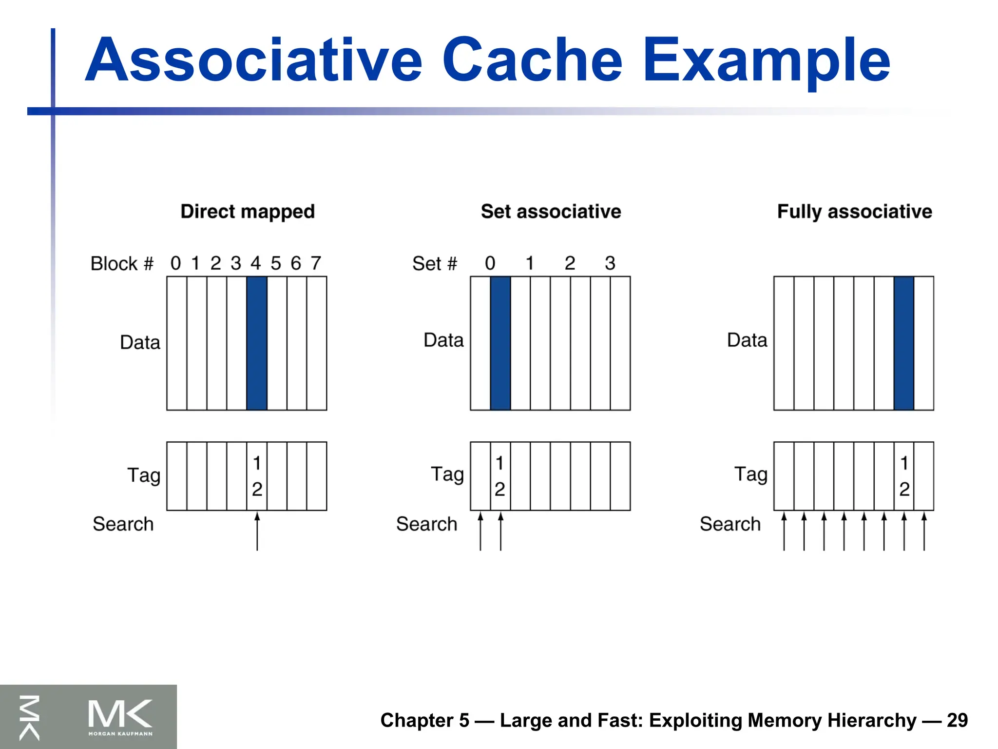
Associative Caches
Fully associative
Allow a given block to go in any cache entry
Requires all entries to be searched at once
Comparator per entry (expensive)
n-way set associative
Each set contains n entries
Block number determines which set
(Block number) modulo (#Sets in cache)
Search all entries in a given set at once
n comparators (less expensive)
164.
Chapter 5 —Large and Fast: Exploiting Memory Hierarchy — 29
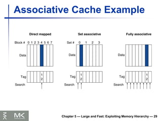
Associative Cache Example
165.
Chapter 5 —Large and Fast: Exploiting Memory Hierarchy — 30
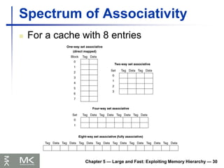
Spectrum of Associativity
For a cache with 8 entries
166.
Chapter 5 —Large and Fast: Exploiting Memory Hierarchy — 31
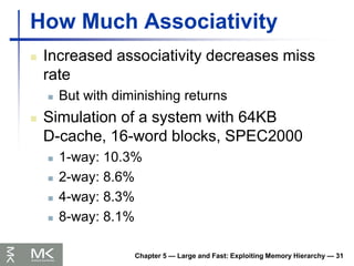
How Much Associativity
Increased associativity decreases miss
rate
But with diminishing returns
Simulation of a system with 64KB
D-cache, 16-word blocks, SPEC2000
1-way: 10.3%
2-way: 8.6%
4-way: 8.3%
8-way: 8.1%
167.
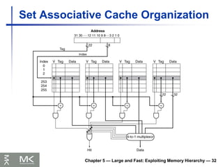
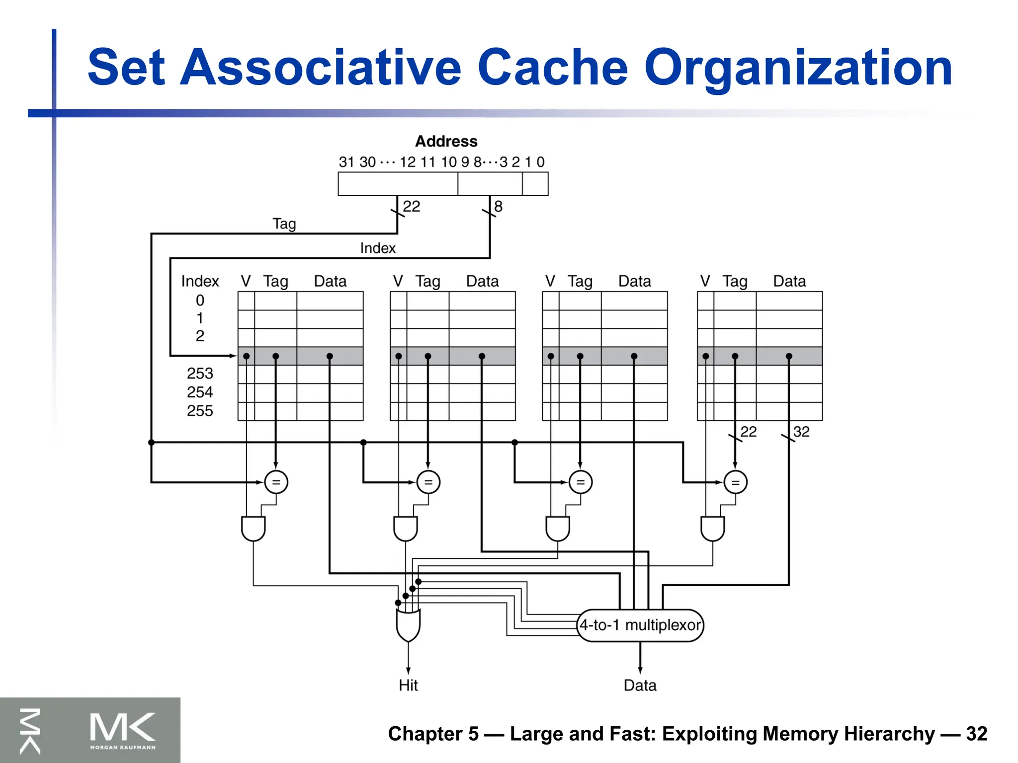
Chapter 5 —Large and Fast: Exploiting Memory Hierarchy — 32
Set Associative Cache Organization
168.
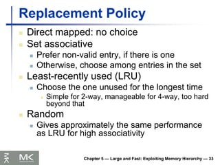
Chapter 5 —Large and Fast: Exploiting Memory Hierarchy — 33
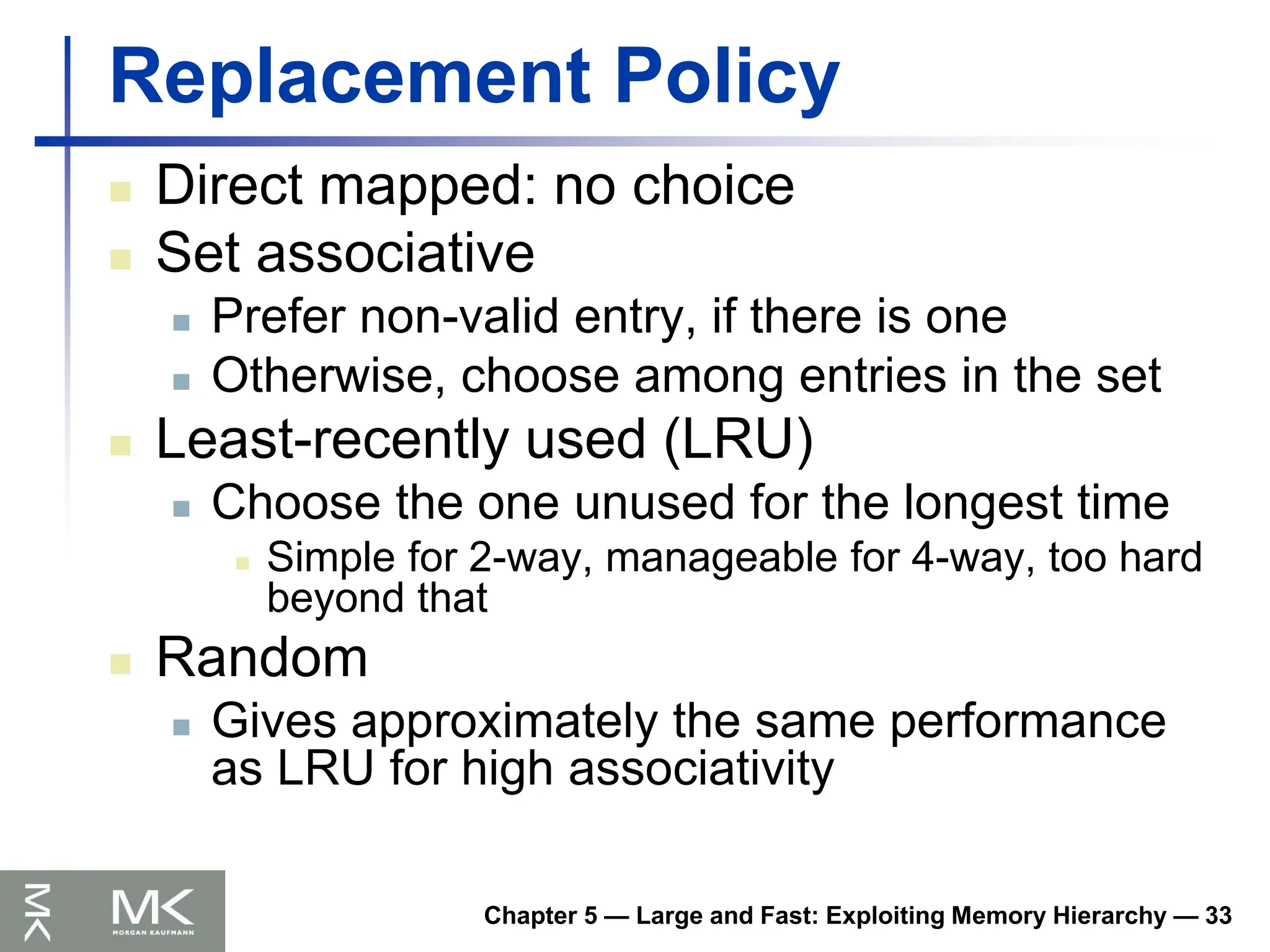
Replacement Policy
Direct mapped: no choice
Set associative
Prefer non-valid entry, if there is one
Otherwise, choose among entries in the set
Least-recently used (LRU)
Choose the one unused for the longest time
Simple for 2-way, manageable for 4-way, too hard
beyond that
Random
Gives approximately the same performance
as LRU for high associativity
Chapter 5 —Large and Fast: Exploiting Memory Hierarchy — 36
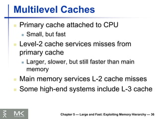
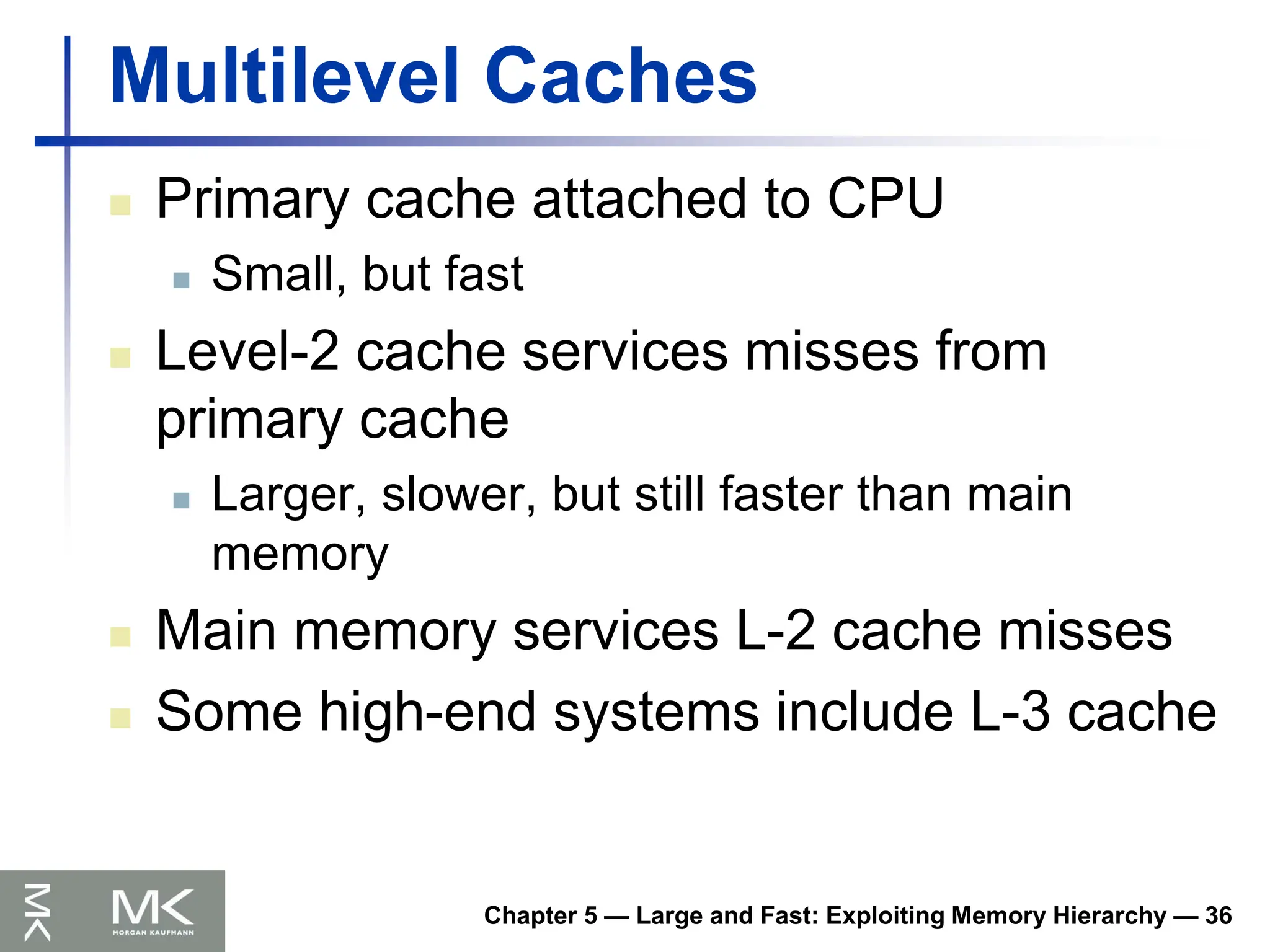
Multilevel Caches
Primary cache attached to CPU
Small, but fast
Level-2 cache services misses from
primary cache
Larger, slower, but still faster than main
memory
Main memory services L-2 cache misses
Some high-end systems include L-3 cache
172.
Chapter 5 —Large and Fast: Exploiting Memory Hierarchy — 37
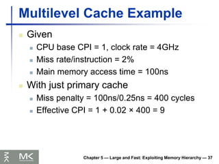
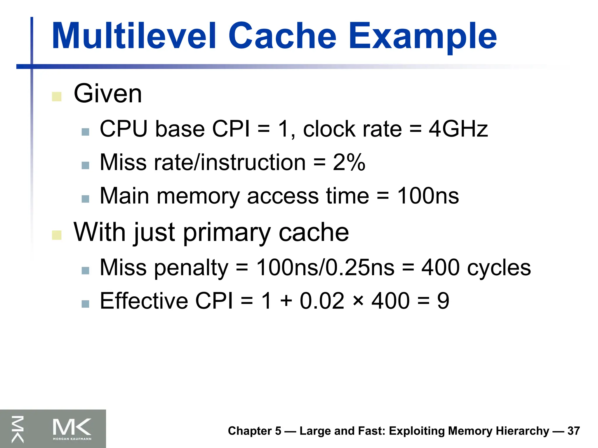
Multilevel Cache Example
Given
CPU base CPI = 1, clock rate = 4GHz
Miss rate/instruction = 2%
Main memory access time = 100ns
With just primary cache
Miss penalty = 100ns/0.25ns = 400 cycles
Effective CPI = 1 + 0.02 × 400 = 9
173.
Chapter 5 —Large and Fast: Exploiting Memory Hierarchy — 38
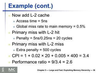
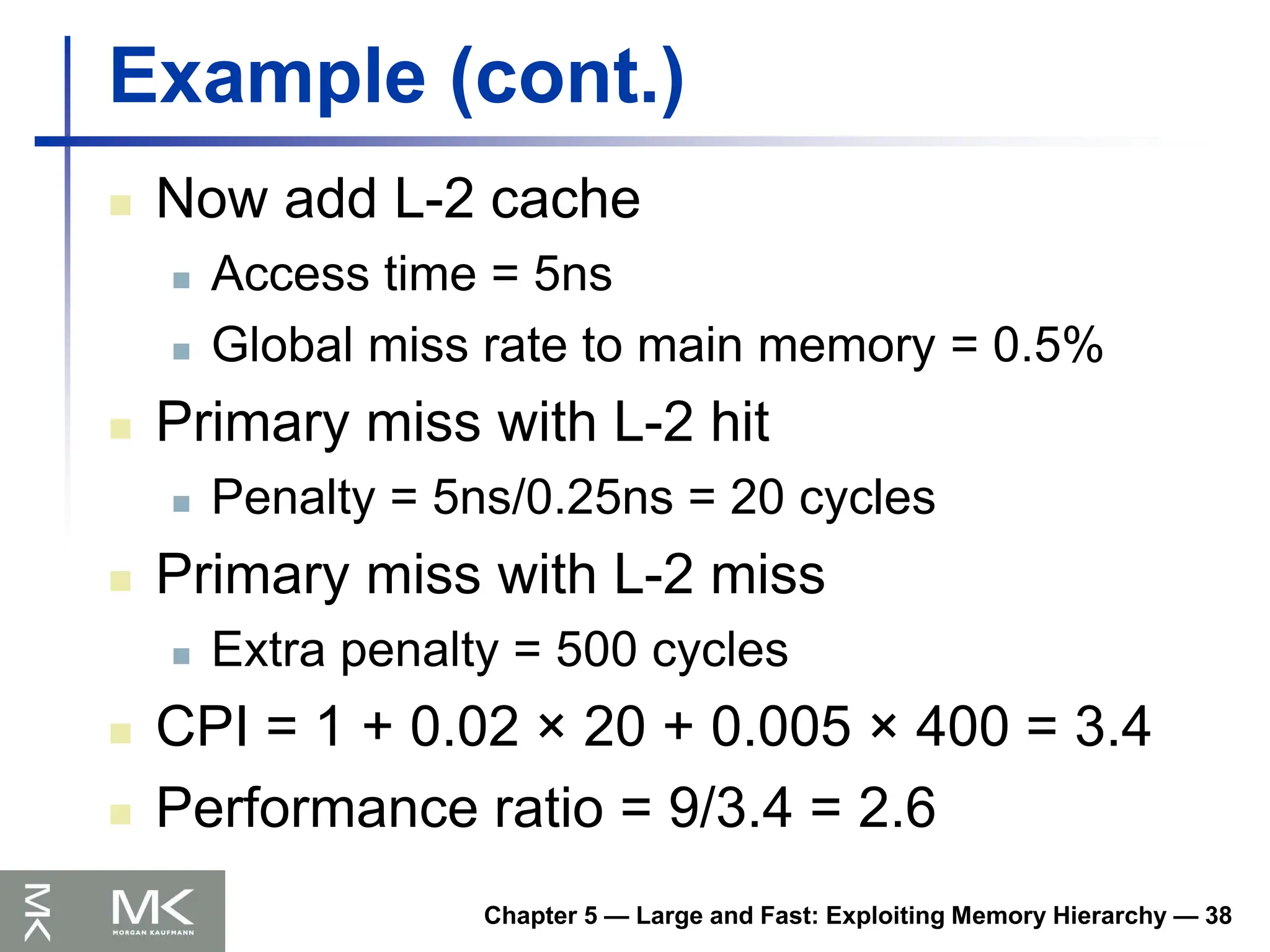
Example (cont.)
Now add L-2 cache
Access time = 5ns
Global miss rate to main memory = 0.5%
Primary miss with L-2 hit
Penalty = 5ns/0.25ns = 20 cycles
Primary miss with L-2 miss
Extra penalty = 500 cycles
CPI = 1 + 0.02 × 20 + 0.005 × 400 = 3.4
Performance ratio = 9/3.4 = 2.6


![Chapter 2 — Instructions: Language of the Computer — 7
Memory Operand Example 1
C code:
g = h + A[8];
g in $s1, h in $s2, base address of A in $s3
Compiled MIPS code:
Index 8 requires offset of 32
4 bytes per word
lw $t0, 32($s3) # load word
add $s1, $s2, $t0
offset base register](https://image.slidesharecdn.com/lecture1-250502192217-1b6f3f2b/85/Lecture-1-Advanced-Computer-Architecture-51-320.jpg)
![Chapter 2 — Instructions: Language of the Computer — 8
Memory Operand Example 2
C code:
A[12] = h + A[8];
h in $s2, base address of A in $s3
Compiled MIPS code:
Index 8 requires offset of 32
lw $t0, 32($s3) # load word
add $t0, $s2, $t0
sw $t0, 48($s3) # store word](https://image.slidesharecdn.com/lecture1-250502192217-1b6f3f2b/85/Lecture-1-Advanced-Computer-Architecture-52-320.jpg)


![Chapter 2 — Instructions: Language of the Computer — 14
Compiling Loop Statements
C code:
while (save[i] == k) i += 1;
i in $s3, k in $s5, address of save in $s6
Compiled MIPS code:
Loop: sll $t1, $s3, 2
add $t1, $t1, $s6
lw $t0, 0($t1)
bne $t0, $s5, Exit
addi $s3, $s3, 1
j Loop
Exit: …](https://image.slidesharecdn.com/lecture1-250502192217-1b6f3f2b/85/Lecture-1-Advanced-Computer-Architecture-58-320.jpg)


![Chapter 2 — Instructions: Language of the Computer — 7
Memory Operand Example 1
C code:
g = h + A[8];
g in $s1, h in $s2, base address of A in $s3
Compiled MIPS code:
Index 8 requires offset of 32
4 bytes per word
lw $t0, 32($s3) # load word
add $s1, $s2, $t0
offset base register](https://image.slidesharecdn.com/lecture1-250502192217-1b6f3f2b/75/Lecture-1-Advanced-Computer-Architecture-51-2048.jpg)
![Chapter 2 — Instructions: Language of the Computer — 8
Memory Operand Example 2
C code:
A[12] = h + A[8];
h in $s2, base address of A in $s3
Compiled MIPS code:
Index 8 requires offset of 32
lw $t0, 32($s3) # load word
add $t0, $s2, $t0
sw $t0, 48($s3) # store word](https://image.slidesharecdn.com/lecture1-250502192217-1b6f3f2b/75/Lecture-1-Advanced-Computer-Architecture-52-2048.jpg)
![Chapter 2 — Instructions: Language of the Computer — 14
Compiling Loop Statements
C code:
while (save[i] == k) i += 1;
i in $s3, k in $s5, address of save in $s6
Compiled MIPS code:
Loop: sll $t1, $s3, 2
add $t1, $t1, $s6
lw $t0, 0($t1)
bne $t0, $s5, Exit
addi $s3, $s3, 1
j Loop
Exit: …](https://image.slidesharecdn.com/lecture1-250502192217-1b6f3f2b/75/Lecture-1-Advanced-Computer-Architecture-58-2048.jpg)


![UiPath Automation Suite Installation (Hands-On) [2/3]](https://cdn.slidesharecdn.com/ss_thumbnails/automationsuitecommunitysession2-251015095633-a6d862f1-thumbnail.jpg?width=600ounds&width=560&fit=bounds)


