Download as PDF, PPTX


The document discusses decision trees as a key classification technique in machine learning, highlighting their structure, advantages, and common terminology. It explains the algorithm's process for creating a tree by recursively selecting attributes to split data based on measures like information gain and Gini index, which assess the purity of data subsets. Constraints on tree size are also addressed, including minimum samples for node splits, maximum depth, and maximum terminal nodes, essential for managing overfitting.
Introduction to Lesson 17 on Classification Techniques focusing on Decision Trees by Kush Kulshrestha.
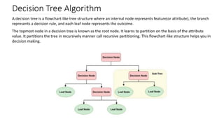
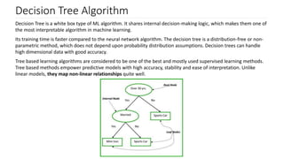
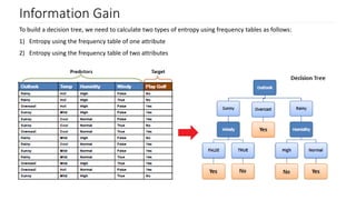
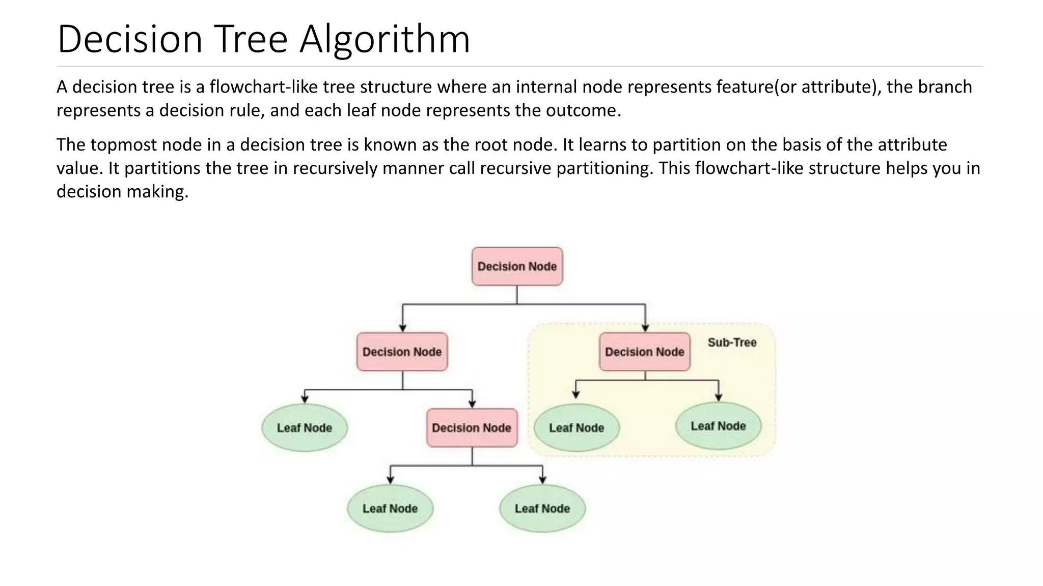
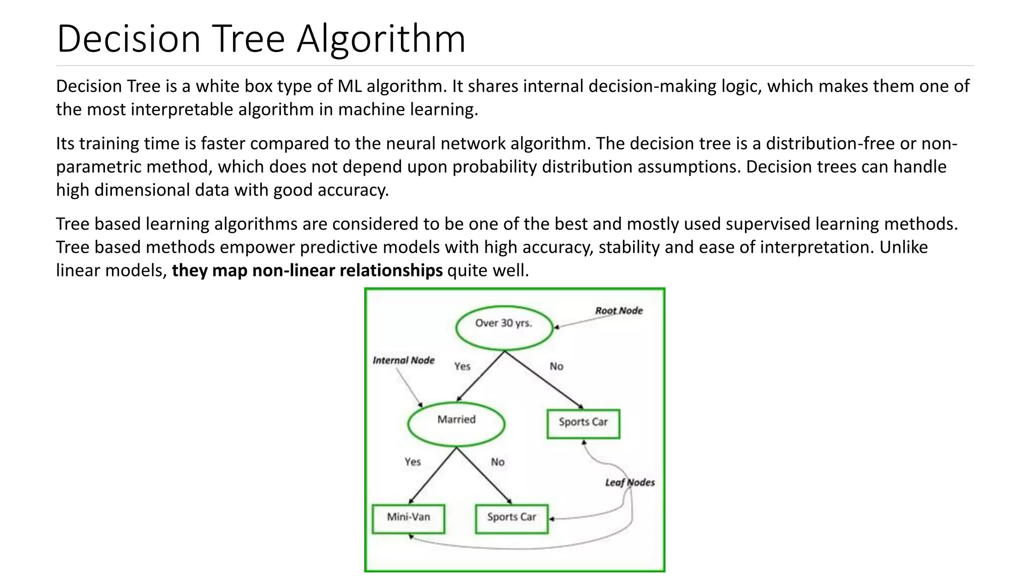
Decision trees as a flowchart-like structure for decision making; notable for interpretability and speed.
Definitions of Common Terms related to decision trees: root node, splitting, decision nodes, and pruning.
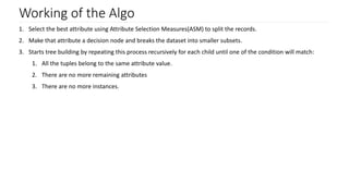
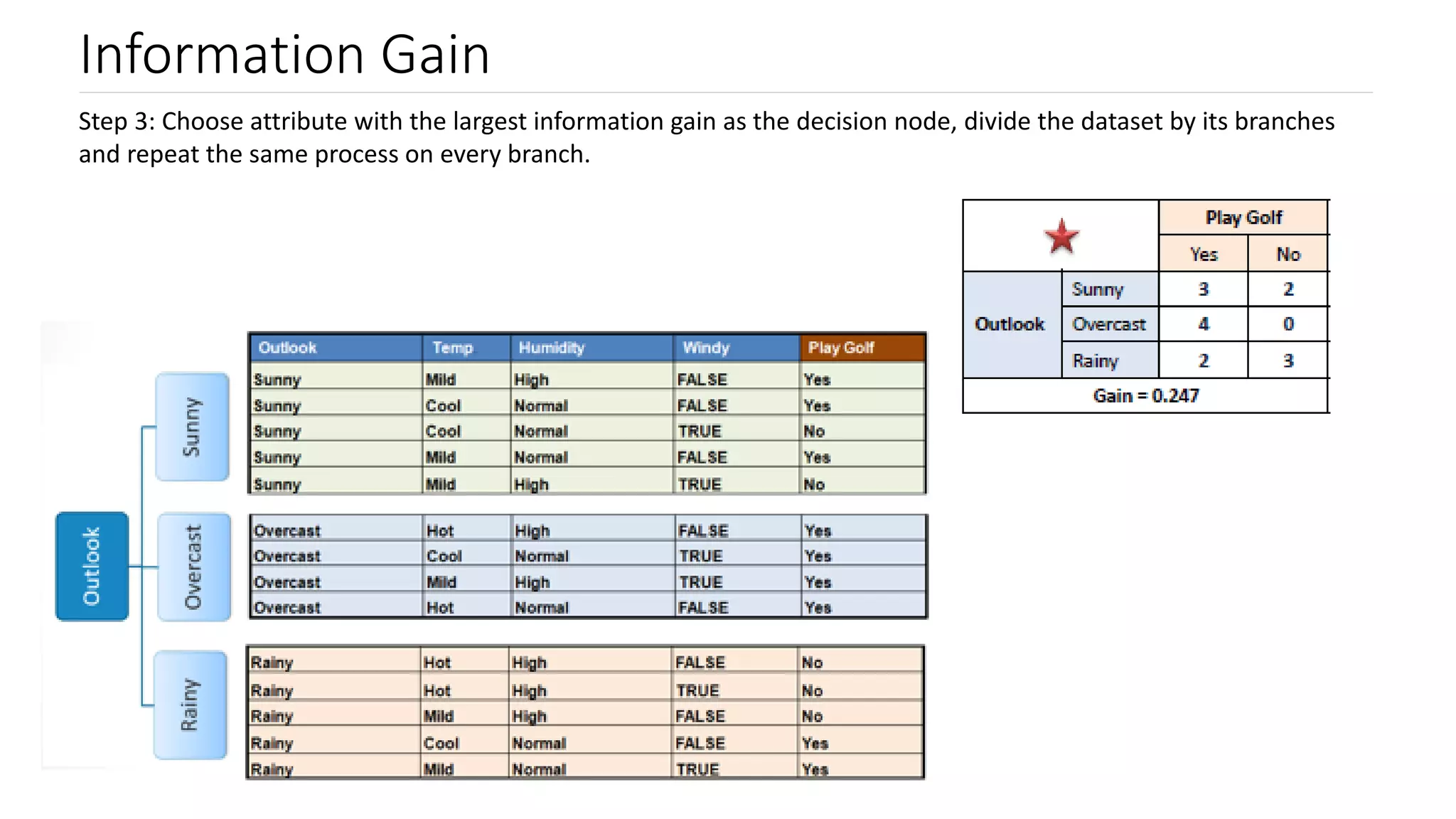
Overview of the algorithm working process involving attribute selection, decision node formation and recursive tree building.
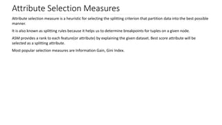
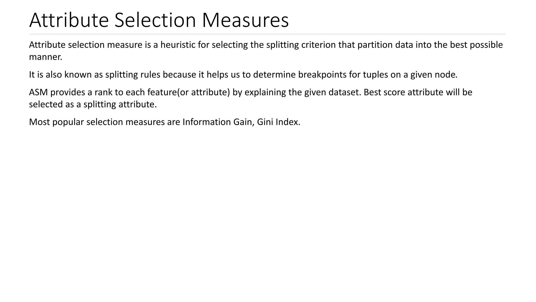
Introduction to Attribute Selection Measures (ASM) for optimizing data partitioning during tree construction.
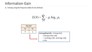
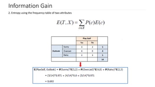
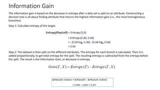
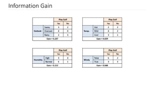
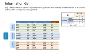
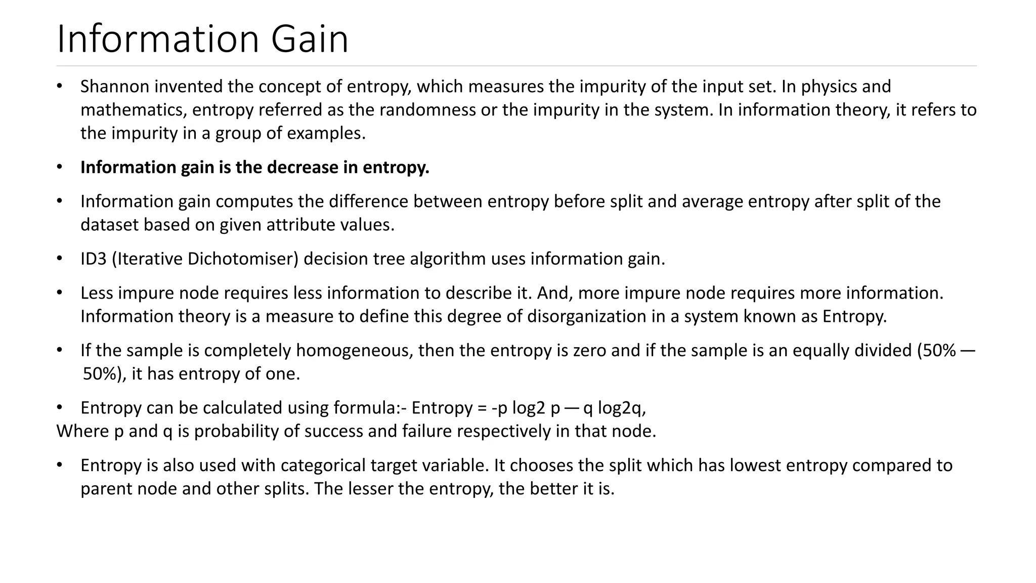
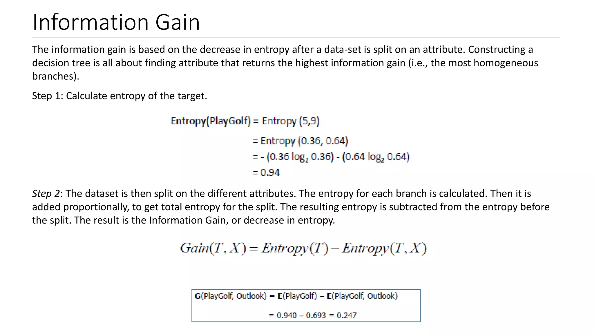
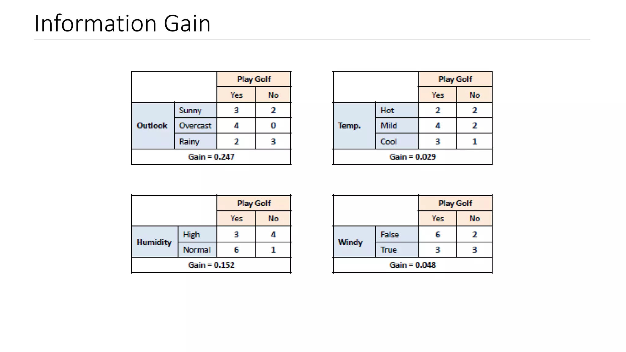
Explanation of Information Gain, its relation to entropy, and how it influences decision tree splits.
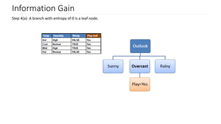
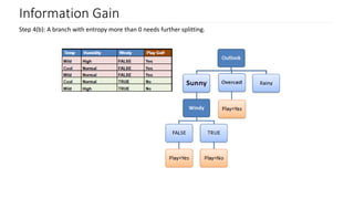
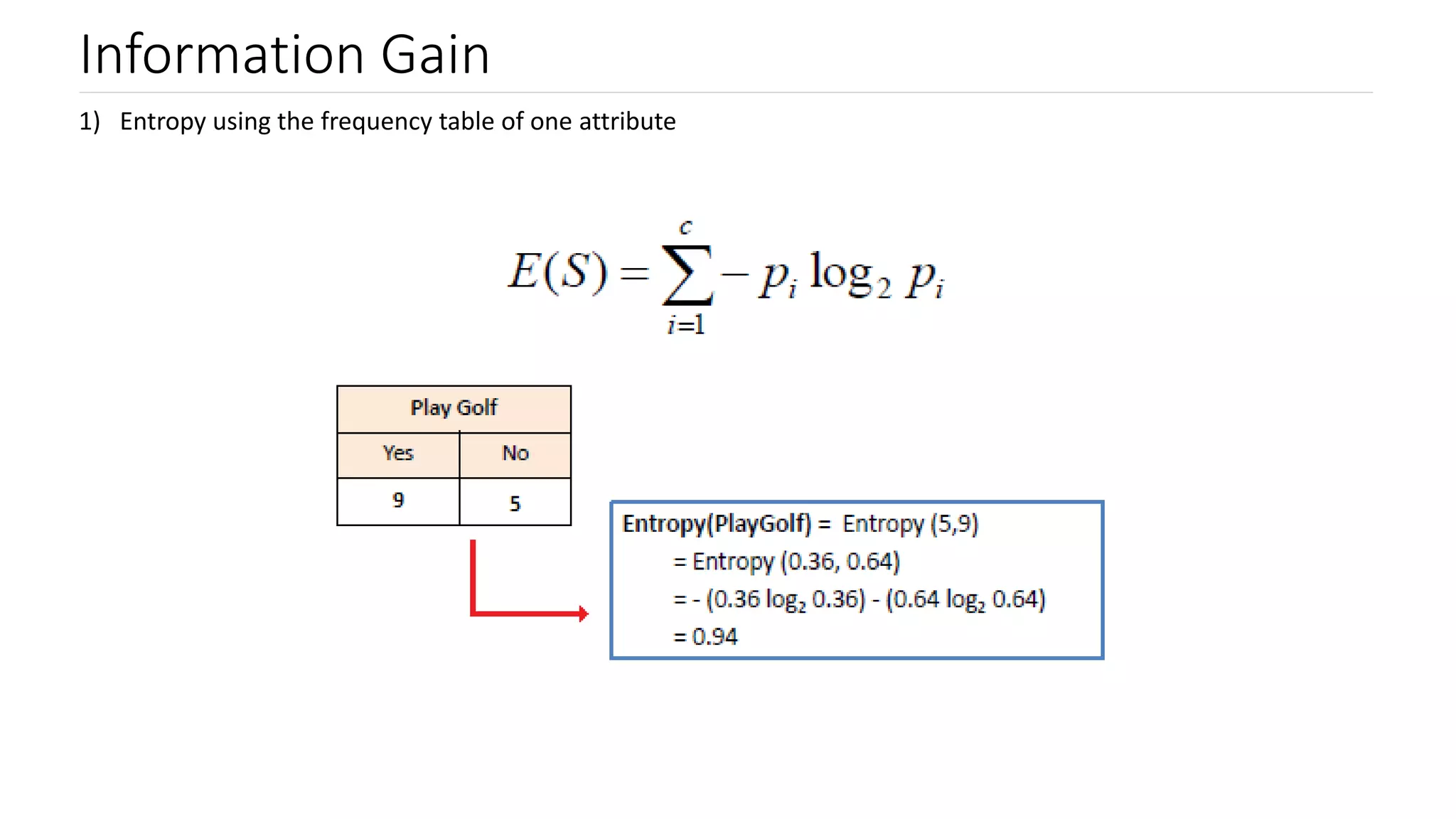
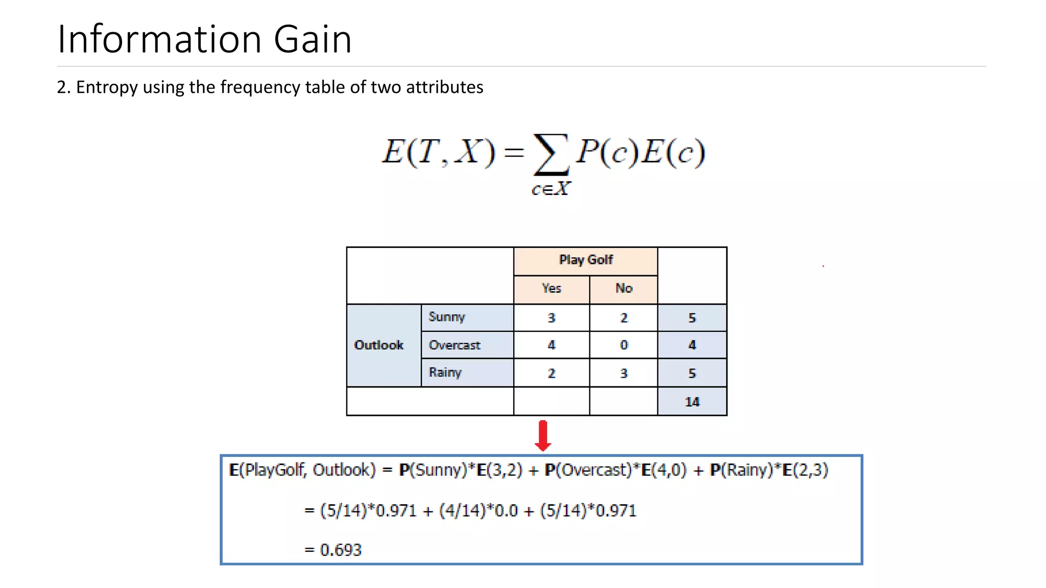
Steps to calculate information gain, focusing on entropy values for determining leaf nodes.
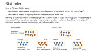
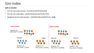
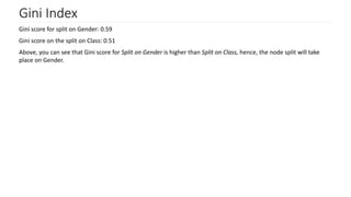
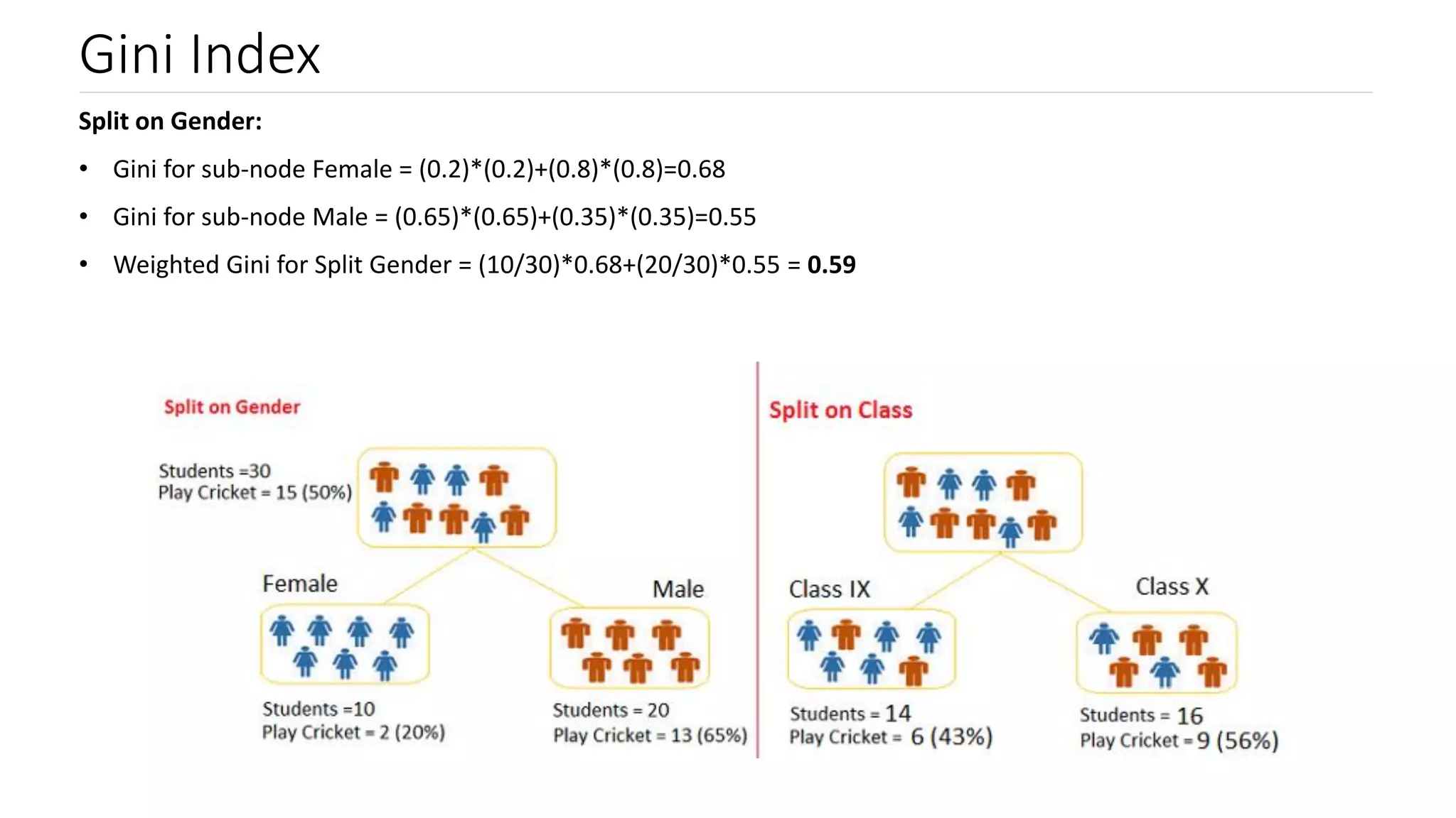
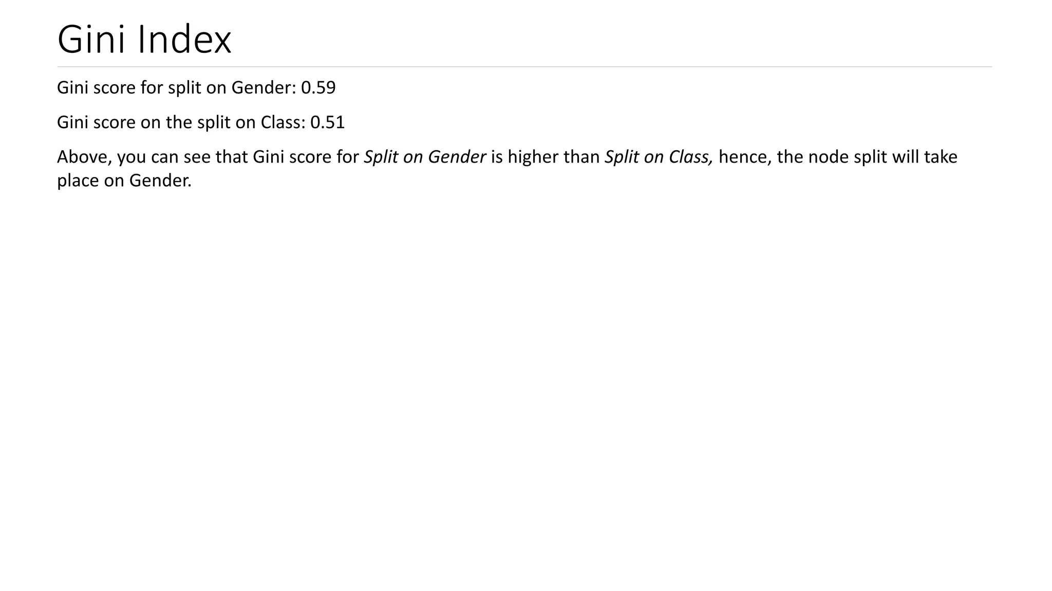
Introduction to Gini Index and its computation; comparing Gini scores for effective node splitting.
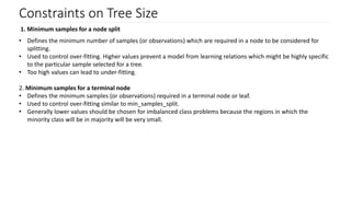
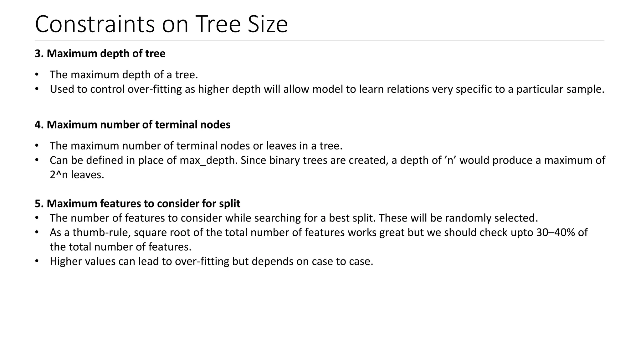
Factors limiting tree size: minimum samples for splits, maximum depth, and features to avoid overfitting.


![Agentic Systems and Compliance - A brief intro [1.2]](https://cdn.slidesharecdn.com/ss_thumbnails/agenticsystemsandcompliace-1-251018025303-958a42ec-thumbnail.jpg?width=600ounds&width=560&fit=bounds)


![Matrix and determinant URT [Autosaved].pptx](https://cdn.slidesharecdn.com/ss_thumbnails/matrixanddeterminanturtautosaved-251018190340-9e6a6deb-thumbnail.jpg?width=600ounds&width=560&fit=bounds)

![RTP_AR_Basic_Learners' Workbook_KS2 [FOR REPRODUCTION] (1).pdf](https://cdn.slidesharecdn.com/ss_thumbnails/rtparbasiclearnersworkbookks2forreproduction1-251016024943-e51a16ac-thumbnail.jpg?width=600ounds&width=560&fit=bounds)


