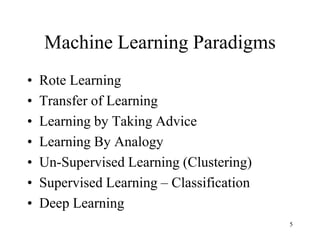
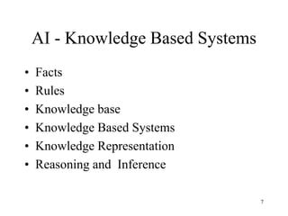
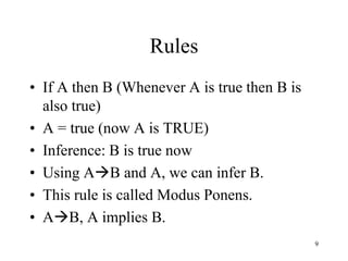
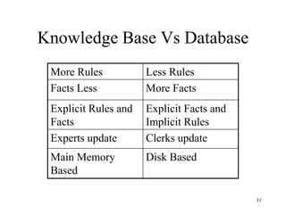
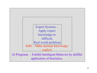
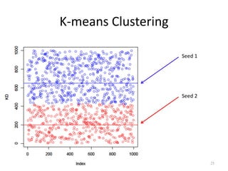
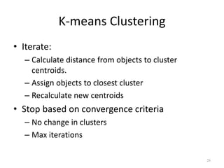
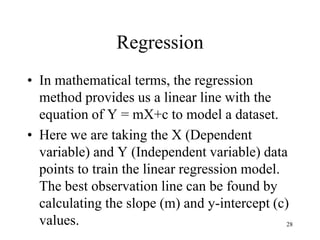
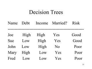
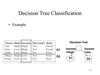
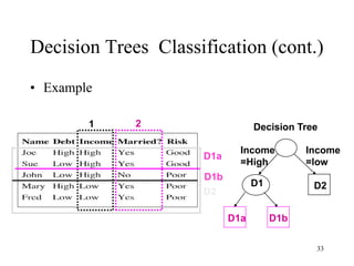
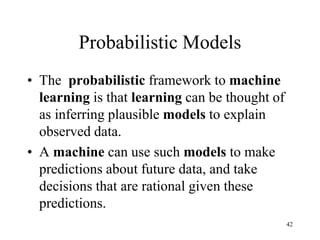
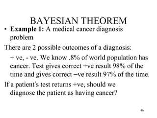
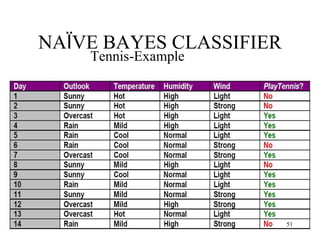
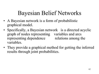
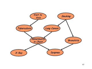
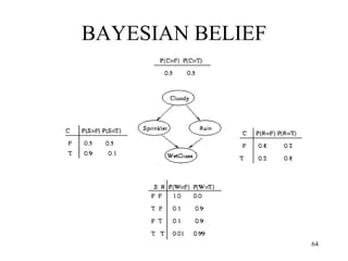
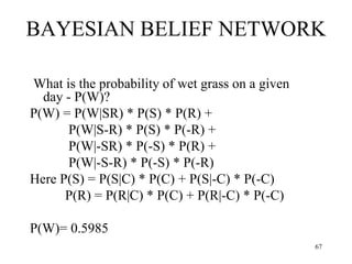
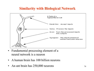
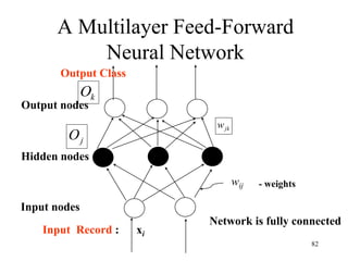
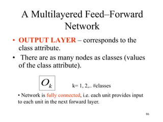
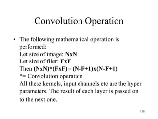
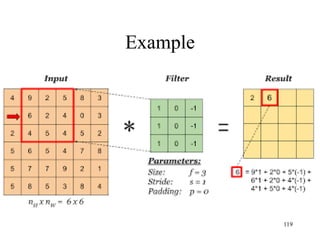
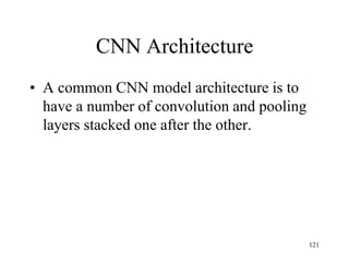
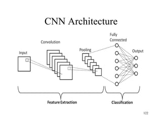
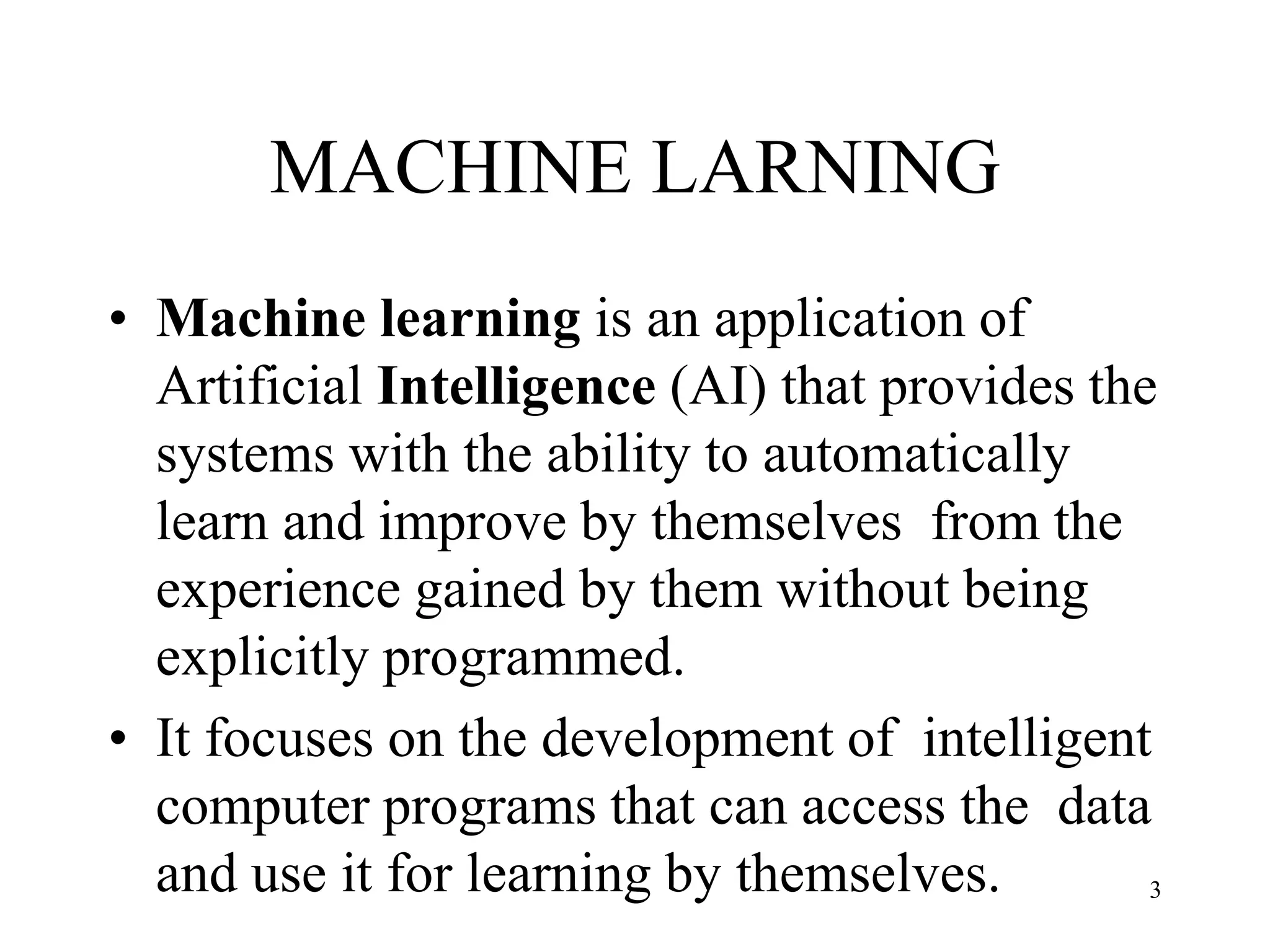
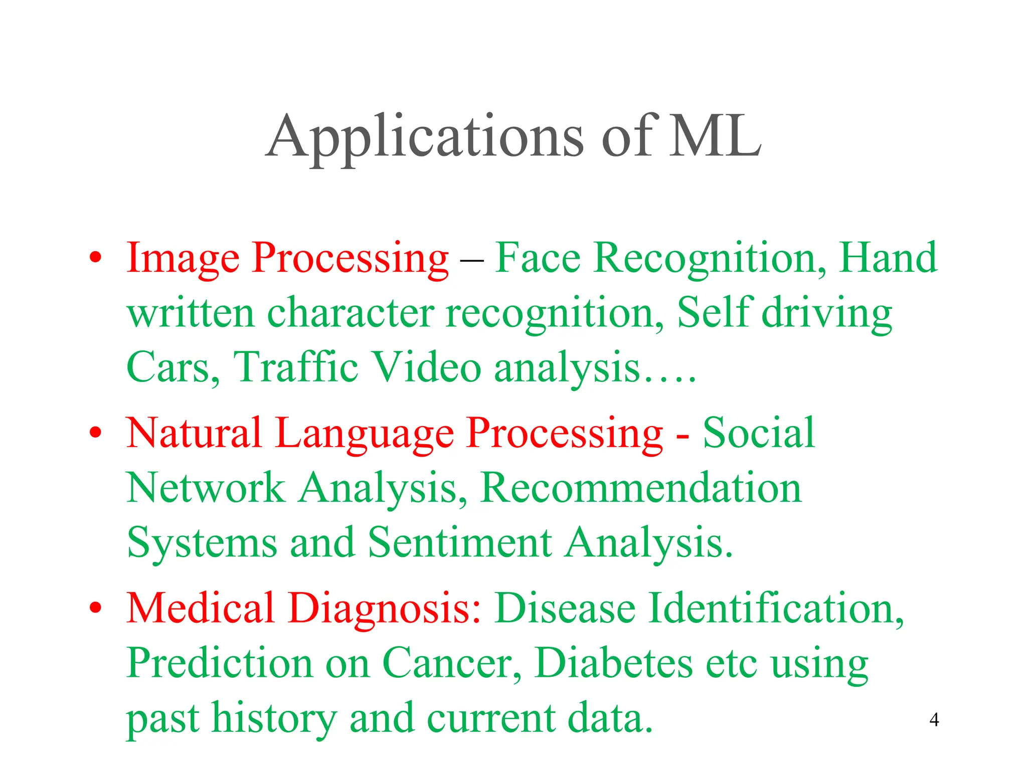
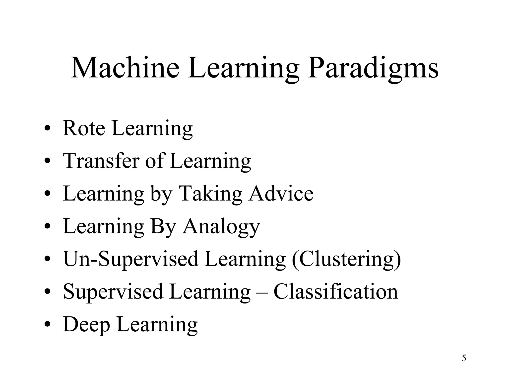
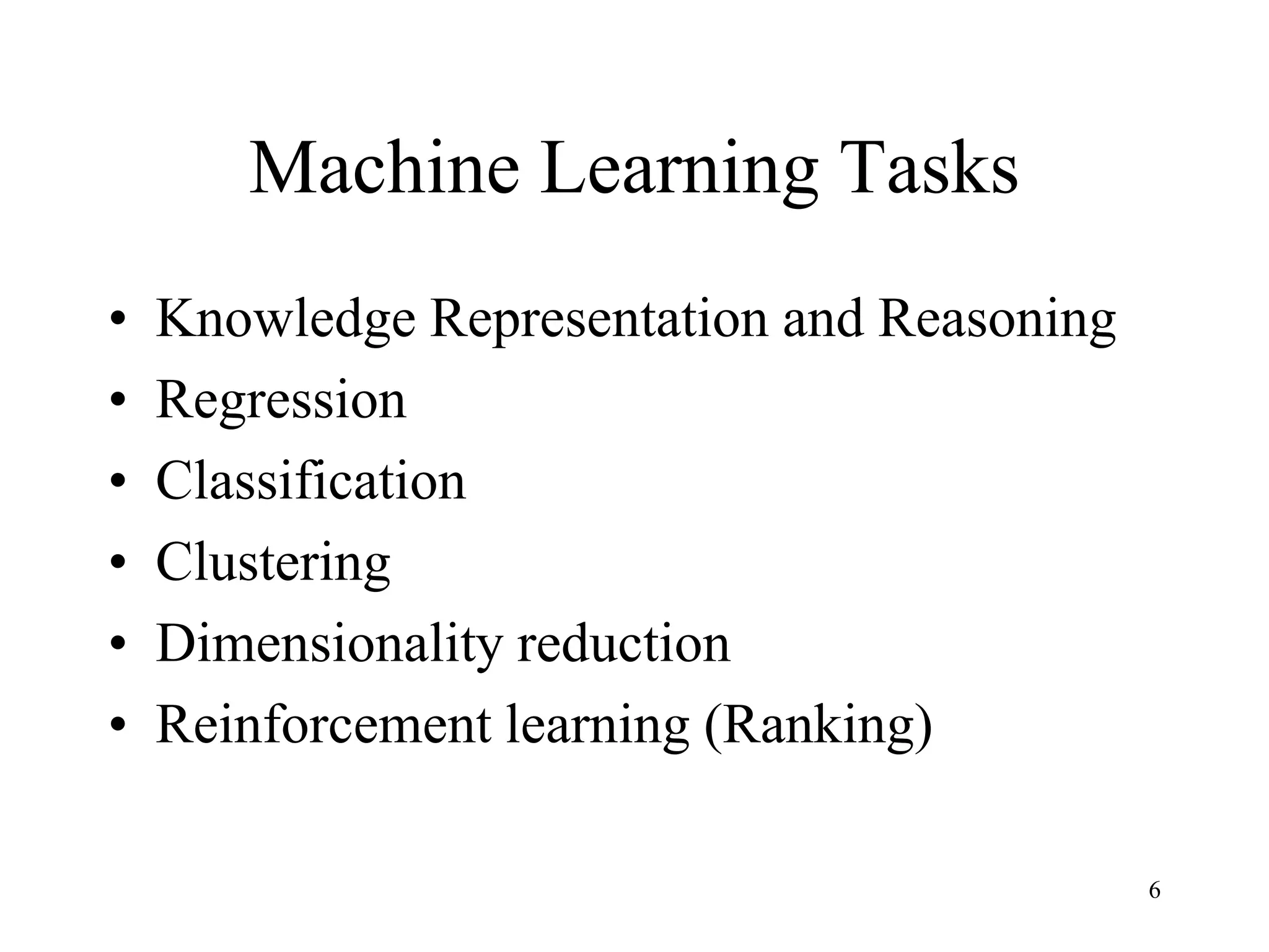
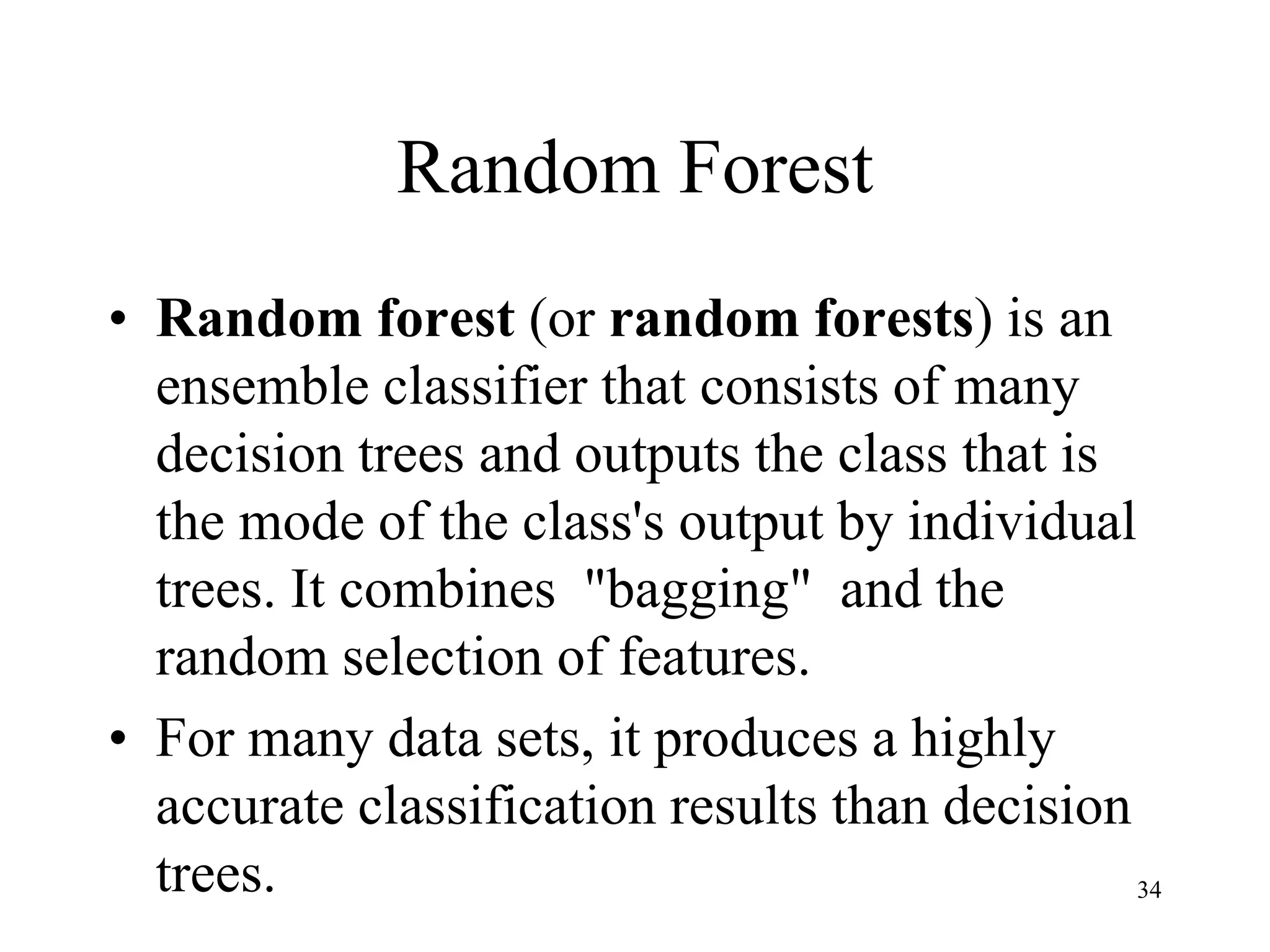
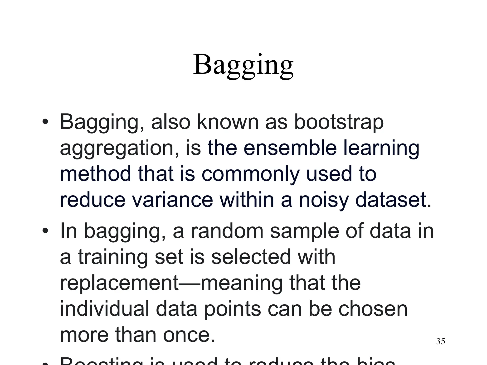
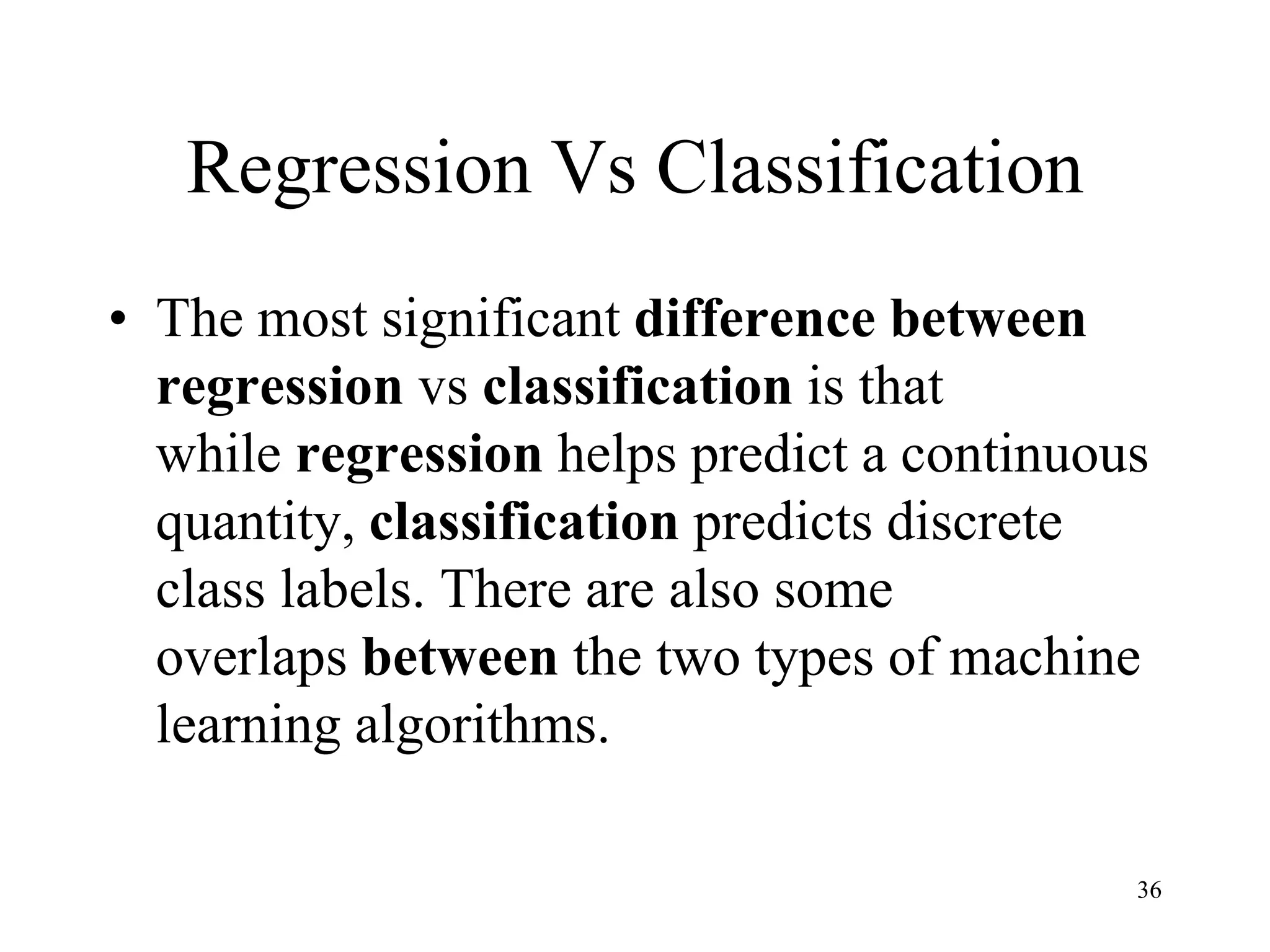
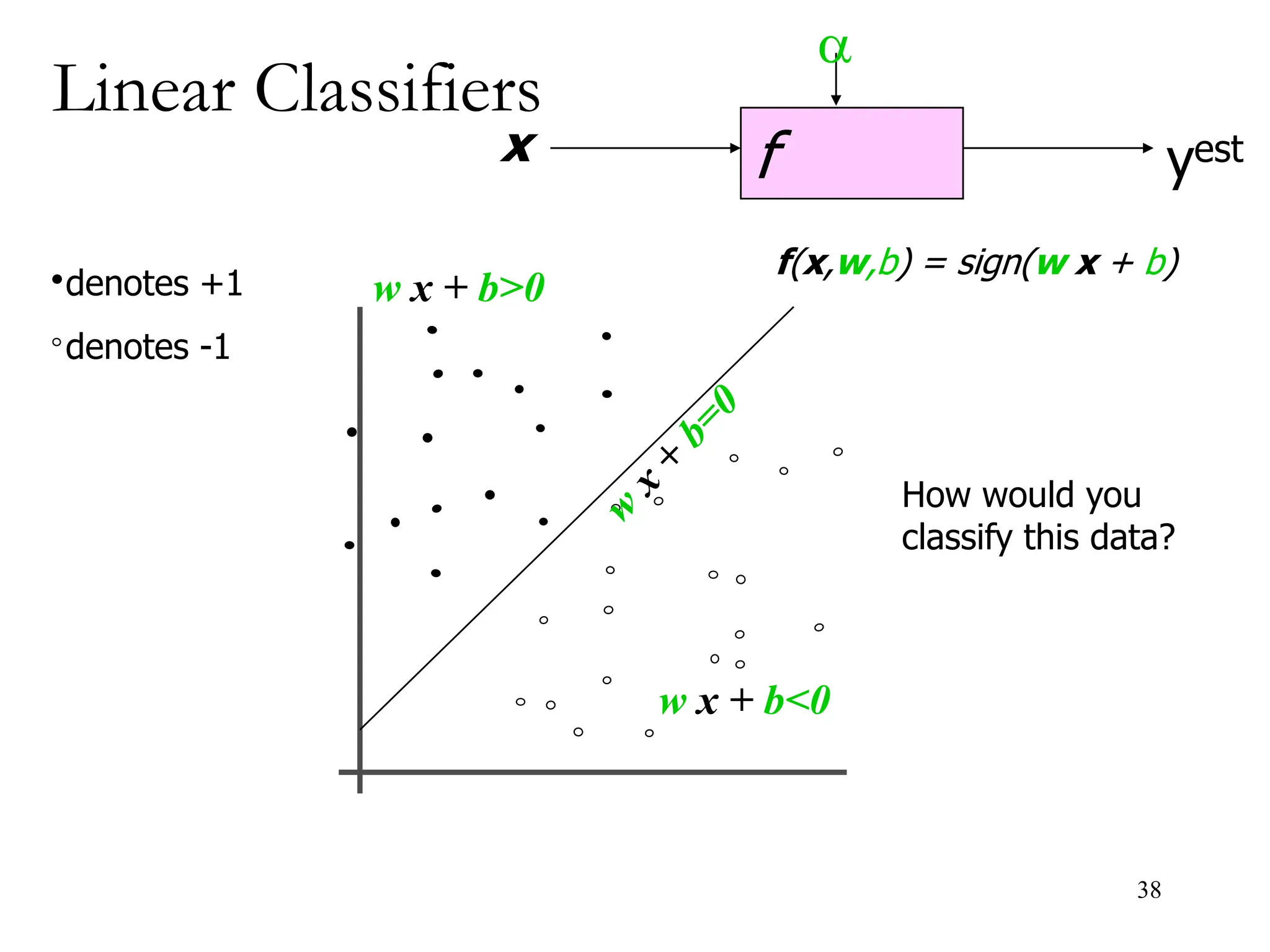
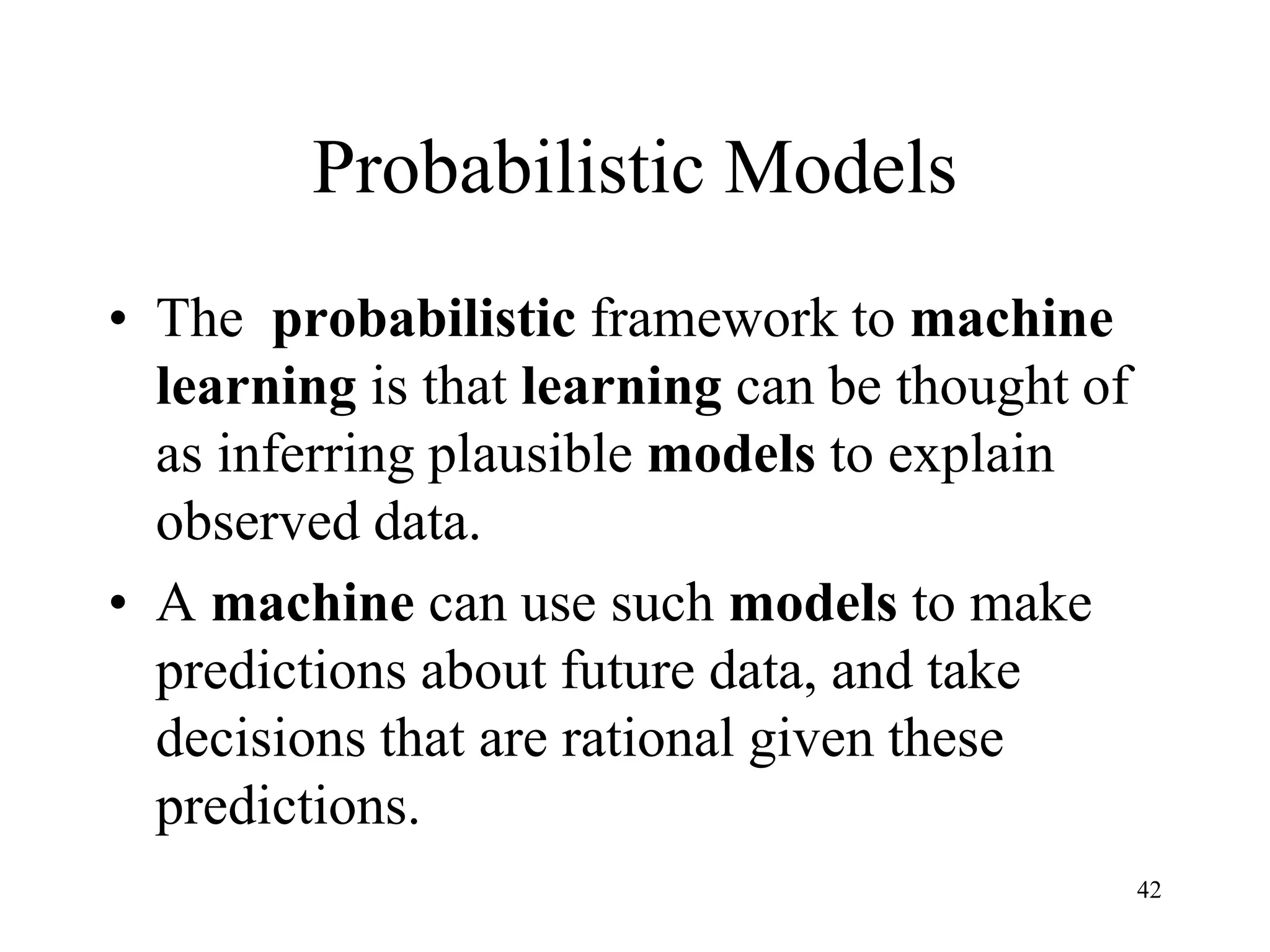
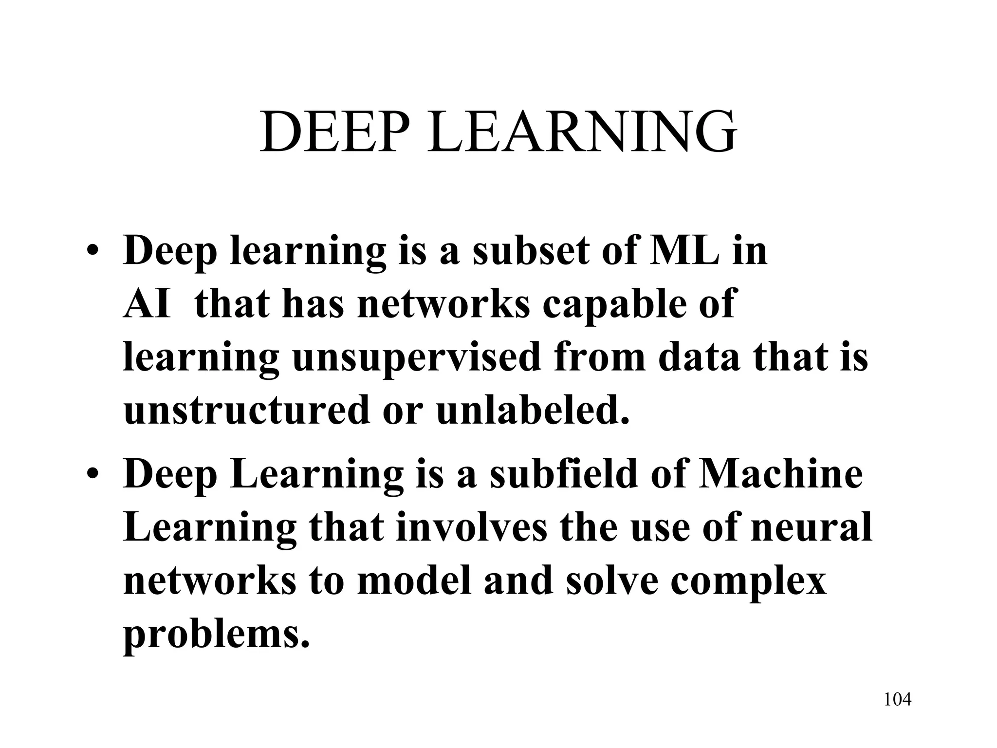
The document discusses the fundamentals of deep learning and machine learning (ML), emphasizing its applications in various fields including image processing, natural language processing, and medical diagnosis. It covers various ML paradigms, tasks, and methods, including supervised and unsupervised learning, regression analysis, decision trees, and Bayesian classification. Additionally, the text explains essential concepts like knowledge representation, reasoning methods, and the importance of probabilistic models in machine learning.


![BAYESIAN THEOREM
• A special case of Bayesian
Theorem:
P(A∩B) = P(B) x P(A|B)
P(B∩A) = P(A) x P(B|A)
Since P(A∩B) = P(B∩A),
P(B) x P(A|B) = P(A) x P(B|A)
=> P(A|B) = [P(A) x P(B|A)] /
P(B)
A
B
P
A
P
A
B
P
A
P
A
B
P
A
P
B
P
A
B
P
A
P
B
A
P
|
|
)
|
(
)
(
)
(
)
|
(
)
(
)
|
(
A B
45](https://image.slidesharecdn.com/2-240709112016-70c3d429/85/Machine-learning-and-deep-learning-algorithms-45-320.jpg)
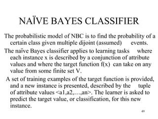
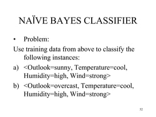
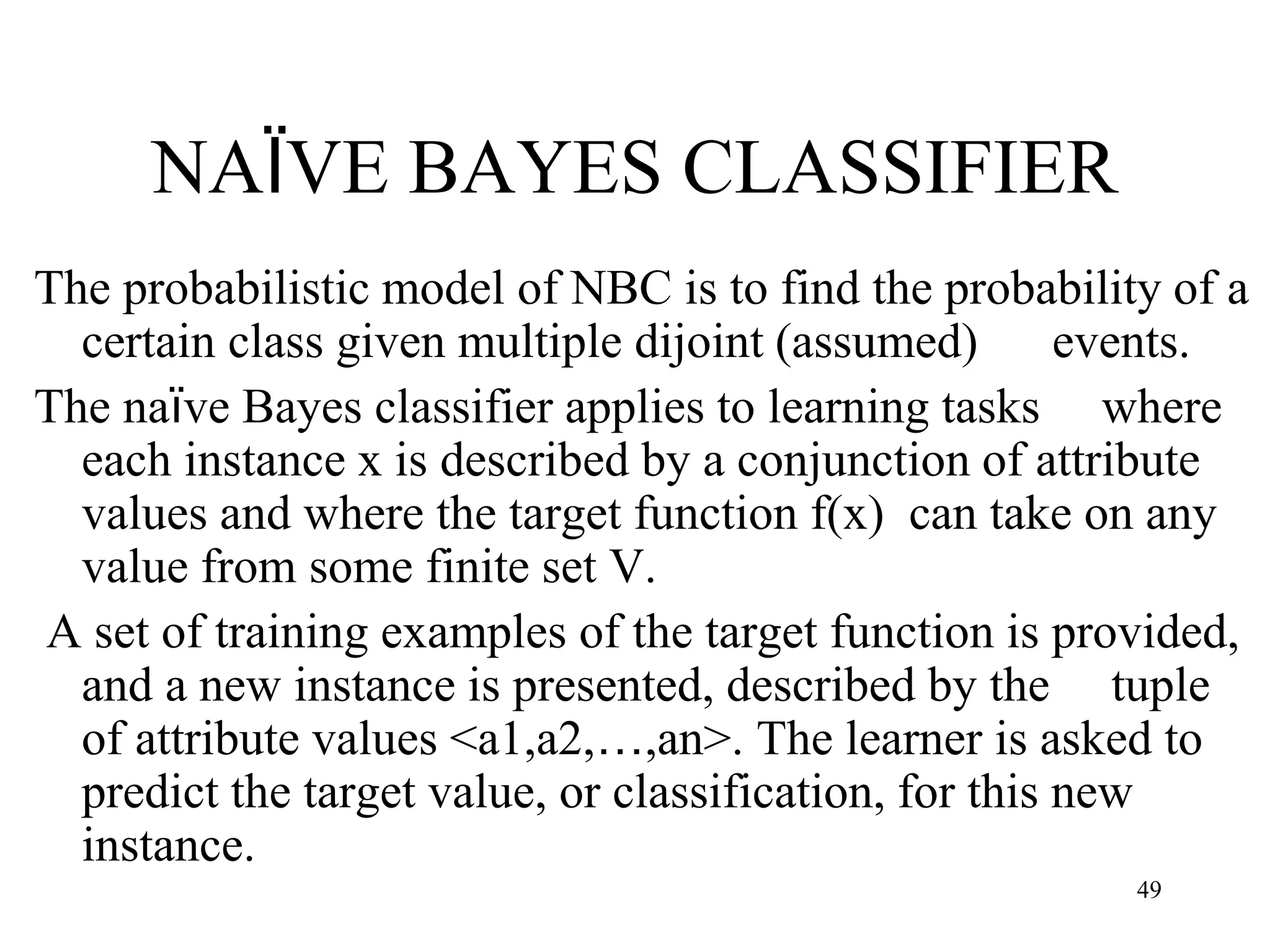
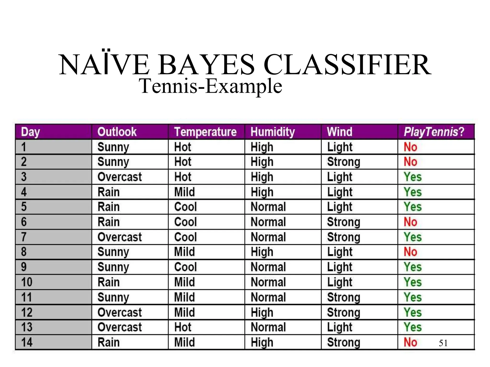
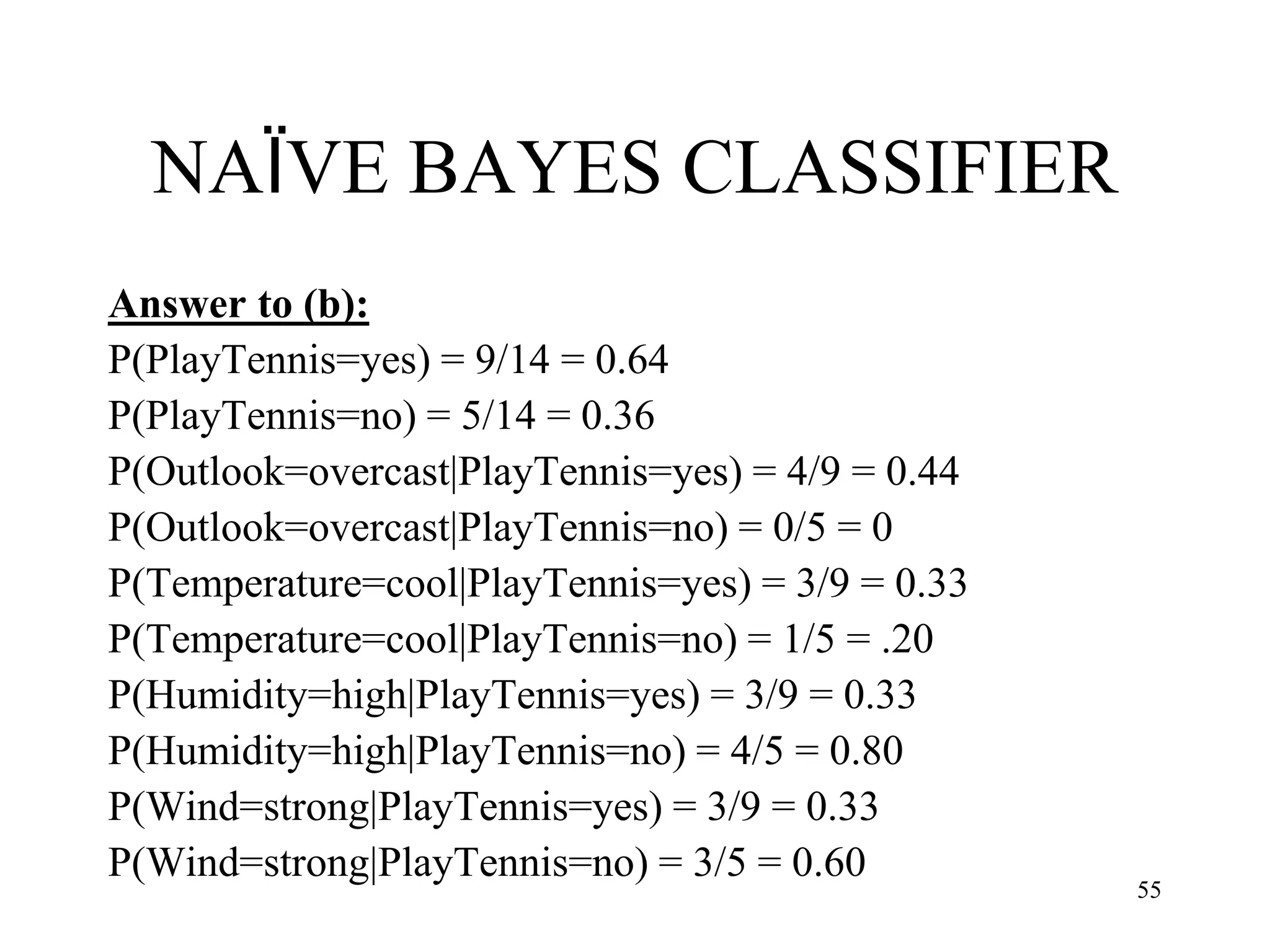
![NAÏVE BAYES CLASSIFIER
Abstractly, probability model for a classifier is a
conditional model
P(C|F1,F2,…,Fn)
Over a dependent class variable C with a small
number of outcome or classes conditional over
several feature variables F1,…,Fn.
Naïve Bayes Formula:
P(C|F1,F2,…,Fn) = argmaxc [P(C) x P(F1|C) x P(F2|C)
x…x P(Fn|C)] / P(F1,F2,…,Fn)
Since P(F1,F2,…,Fn) is common to all probabilities, we
need not evaluate the denominator for comparisons.
50](https://image.slidesharecdn.com/2-240709112016-70c3d429/85/Machine-learning-and-deep-learning-algorithms-50-320.jpg)

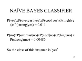
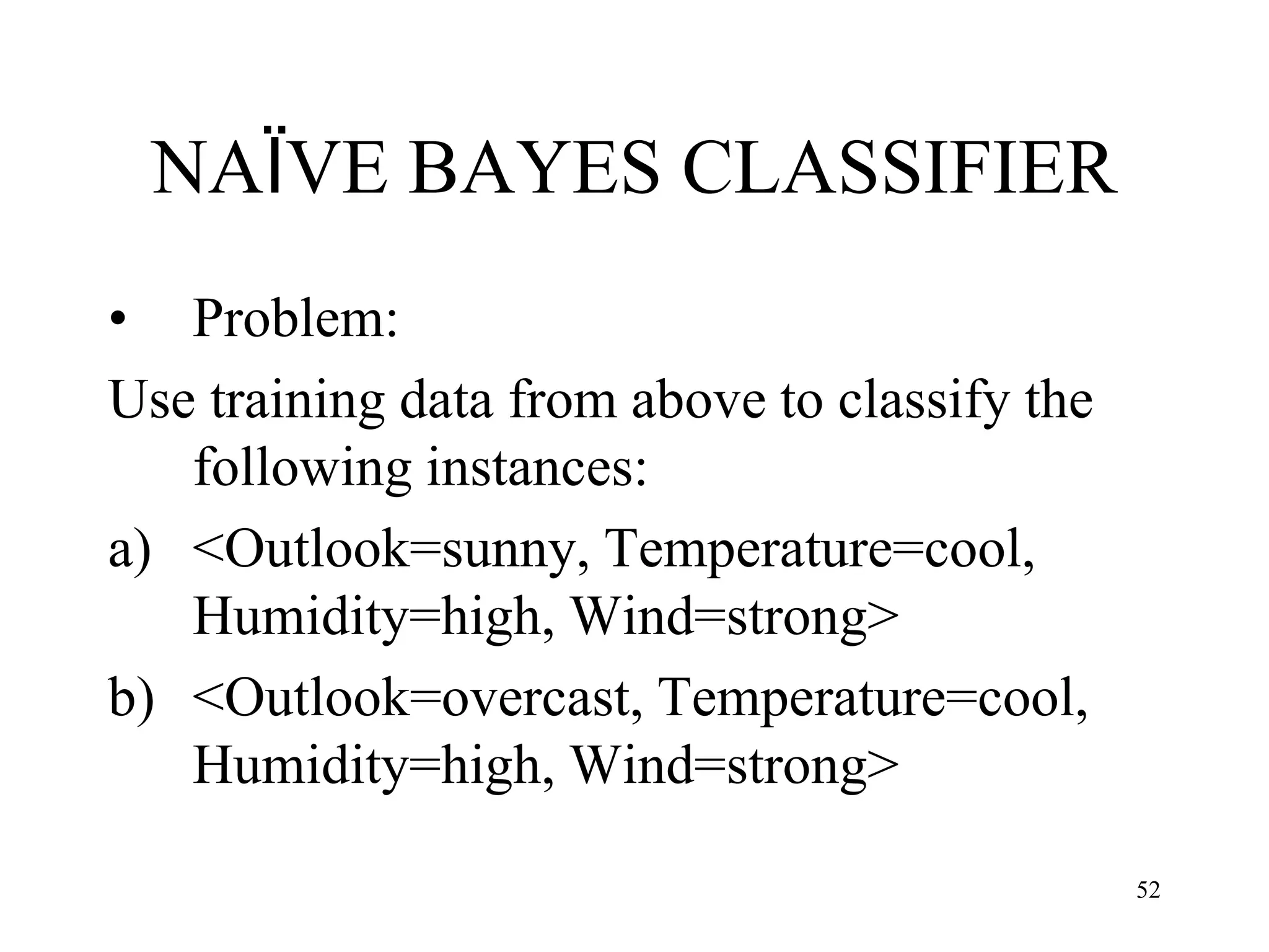
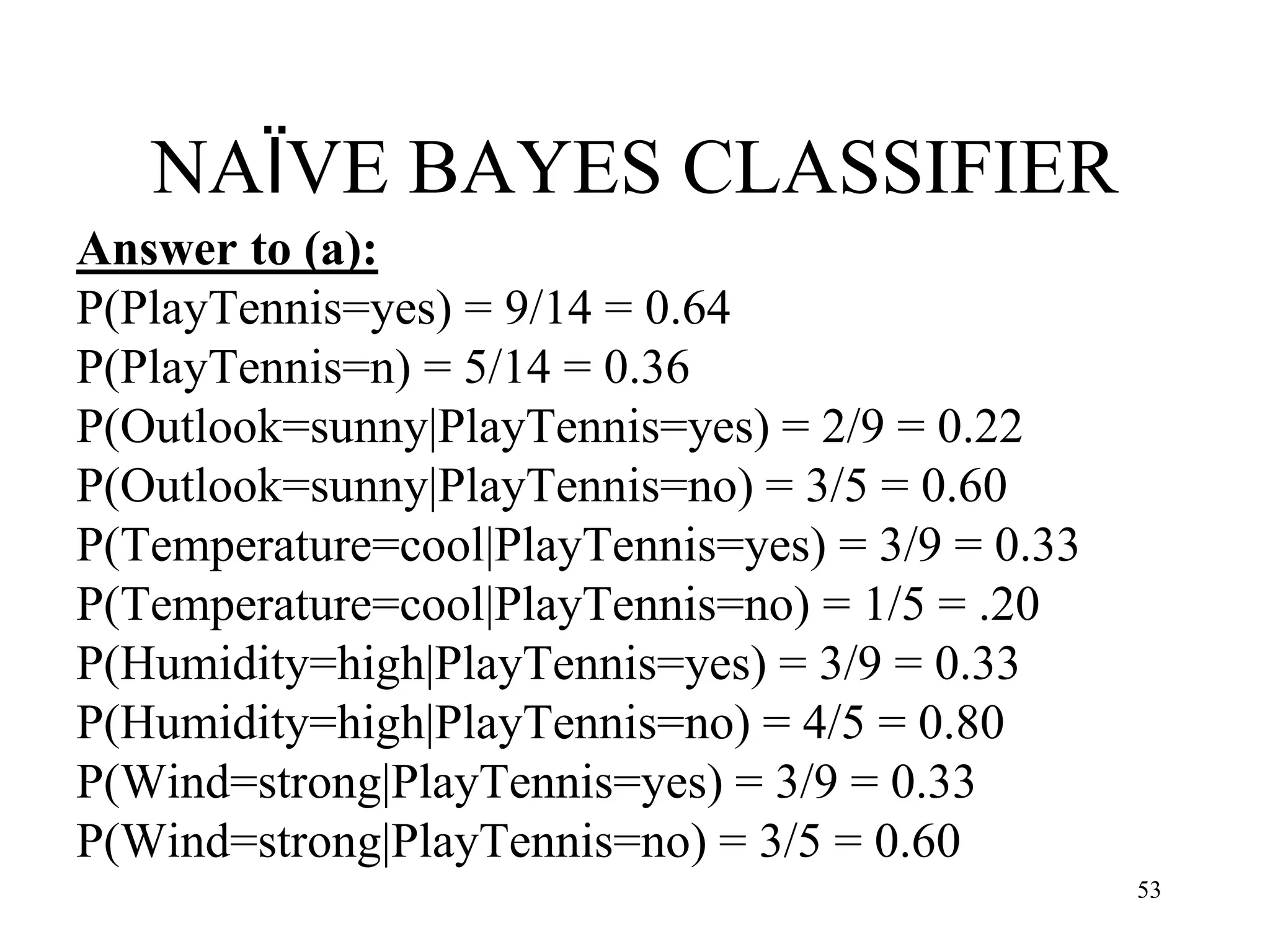
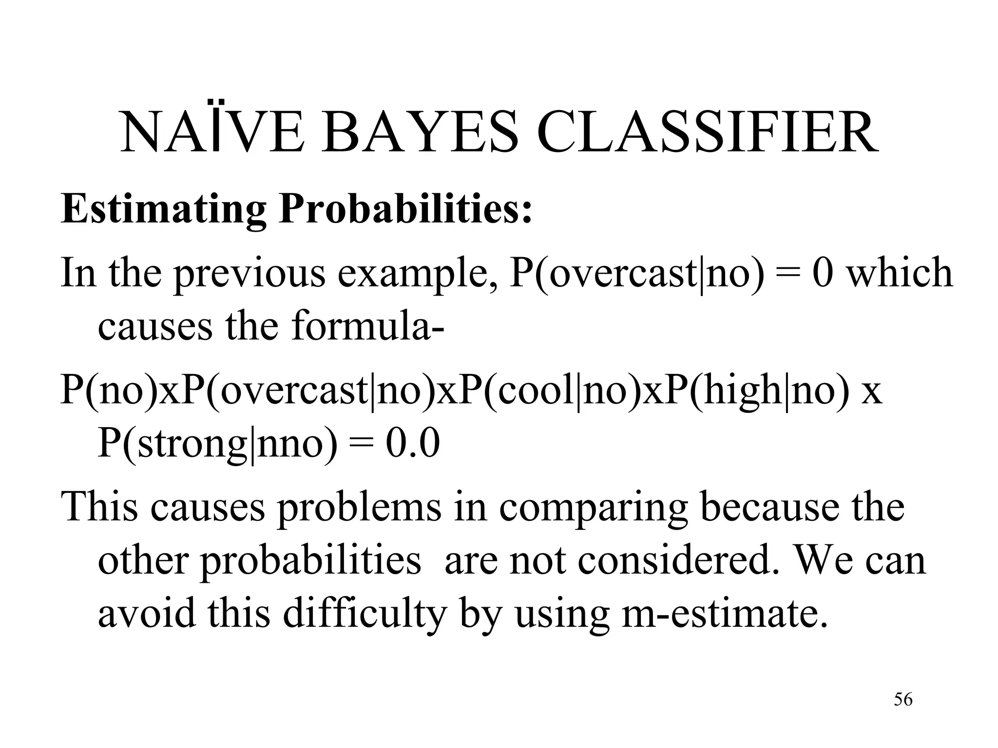
![NAÏVE BAYES CLASSIFIER
P(yes)xP(sunny|yes)xP(cool|yes)xP(high|yes) x
P(strong|yes) = 0.0053
P(no)xP(sunny|no)xP(cool|no)xP(high|no) x
P(strong|no) = 0.0206
So the class for this instance is ‘no’. We can
normalize the probility by:
[0.0206]/[0.0206+0.0053] = 0.795
54](https://image.slidesharecdn.com/2-240709112016-70c3d429/85/Machine-learning-and-deep-learning-algorithms-54-320.jpg)

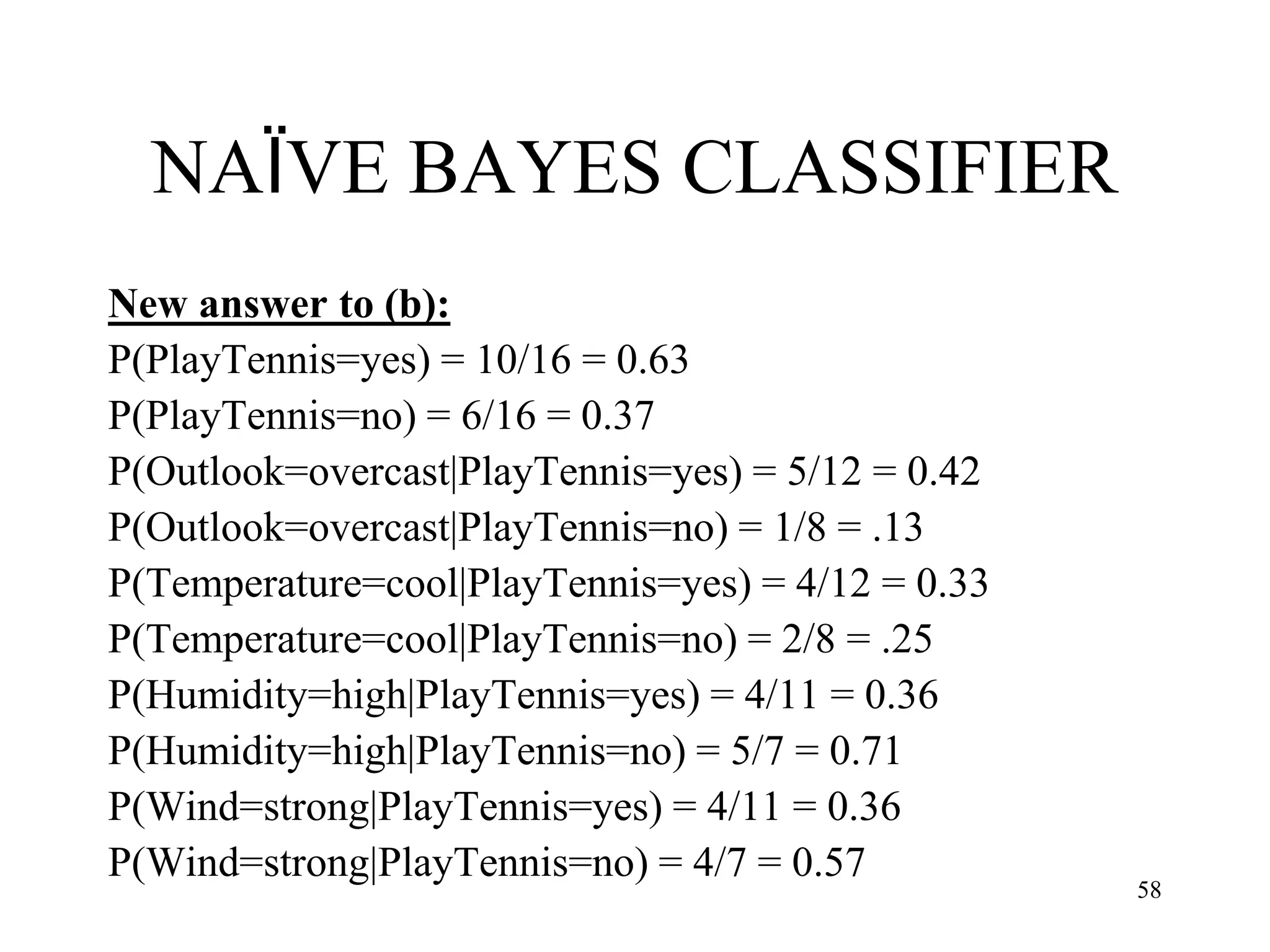
![NAÏVE BAYES CLASSIFIER
M-Estimate Formula:
[c + k] / [n + m] where c/n is the original
probability used before, k=1 and
m= equivalent sample size.
Using this method our new values of
probability is given below-
57](https://image.slidesharecdn.com/2-240709112016-70c3d429/85/Machine-learning-and-deep-learning-algorithms-57-320.jpg)


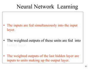
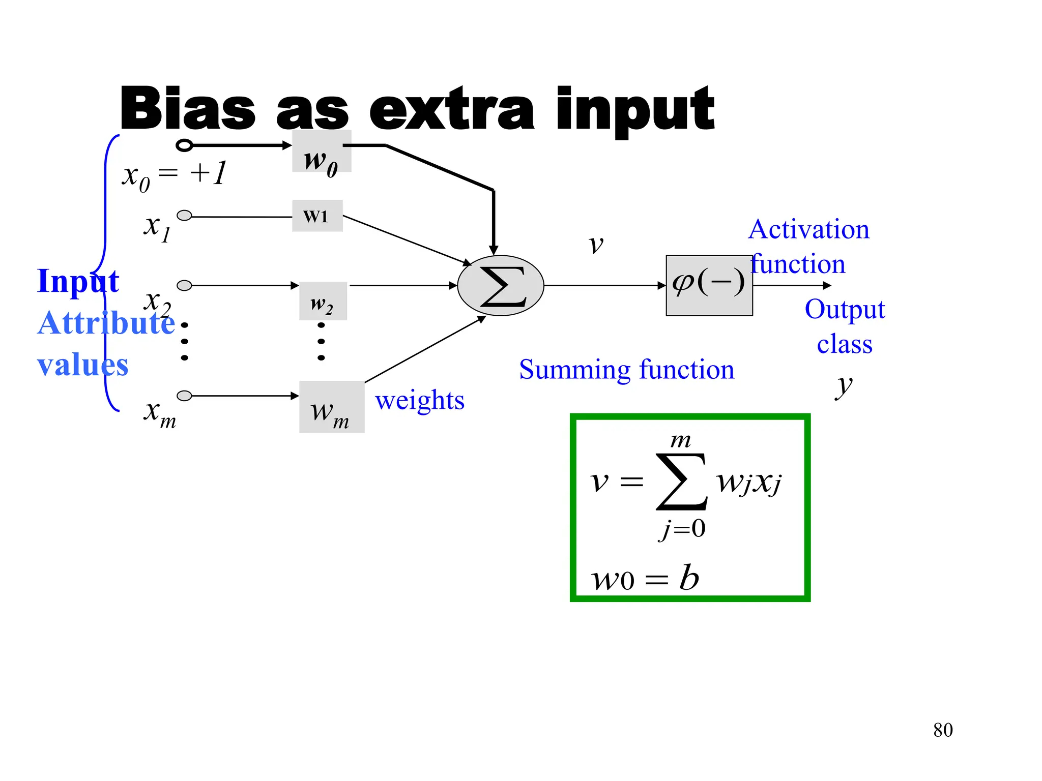
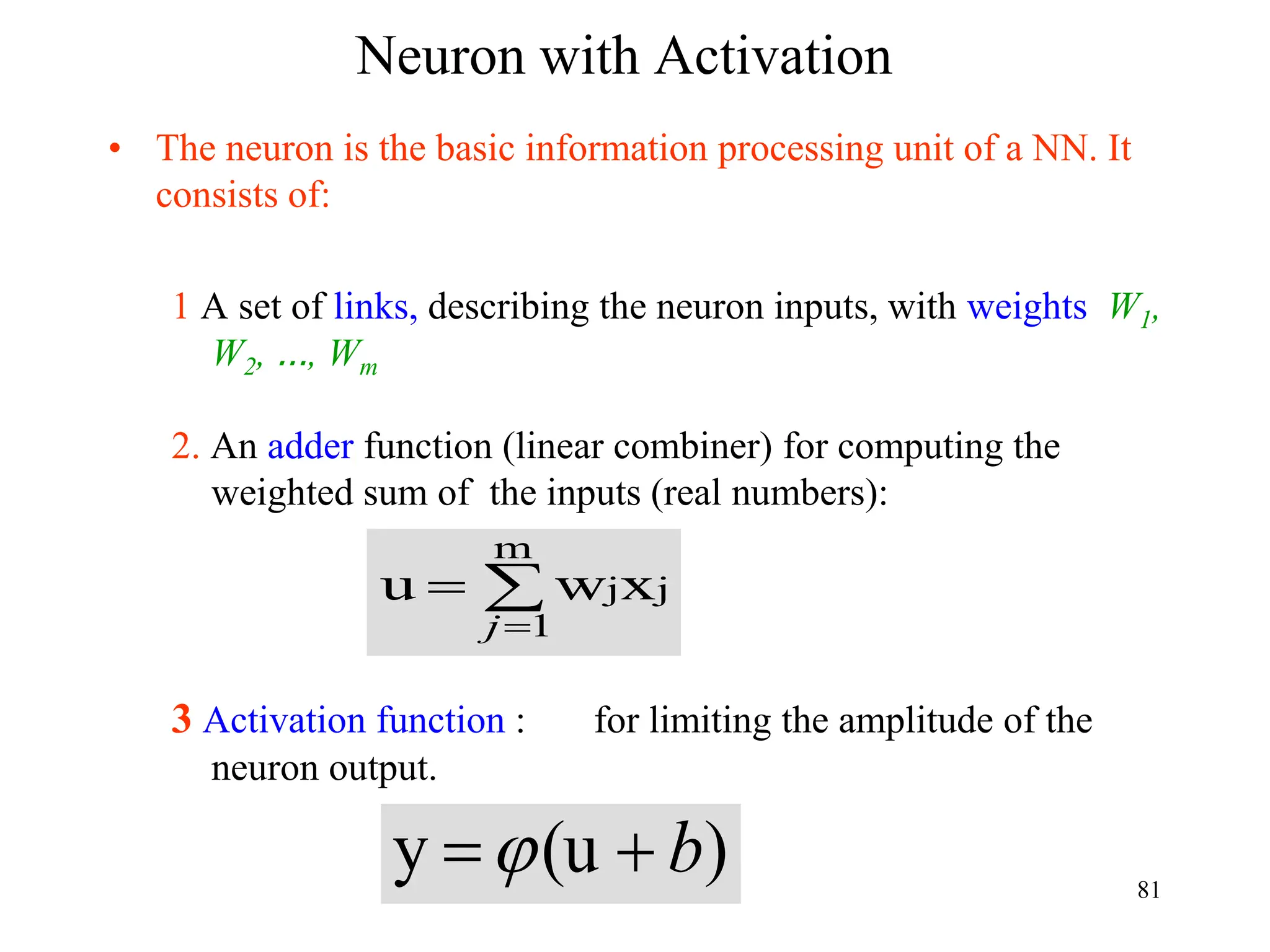
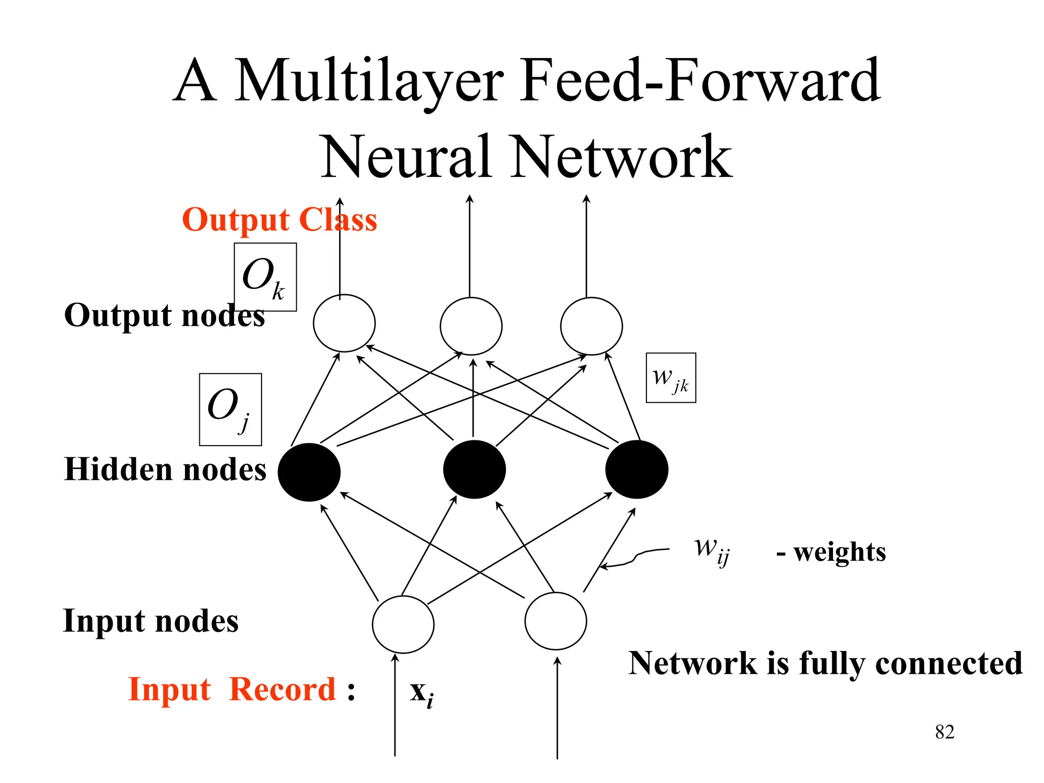
![Neural Network Classifier
• Input: Classification data
It contains classification attribute
• Data is divided, as in any classification problem.
[Training data and Testing data]
• All data must be normalized.
(i.e. all values of attributes in the database are changed to contain values
in the internal [0,1] or[-1,1])
Neural Network can work with data in the range of (0,1) or (-1,1)
77](https://image.slidesharecdn.com/2-240709112016-70c3d429/85/Machine-learning-and-deep-learning-algorithms-77-320.jpg)
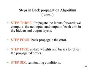
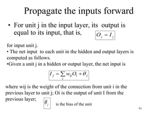
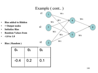
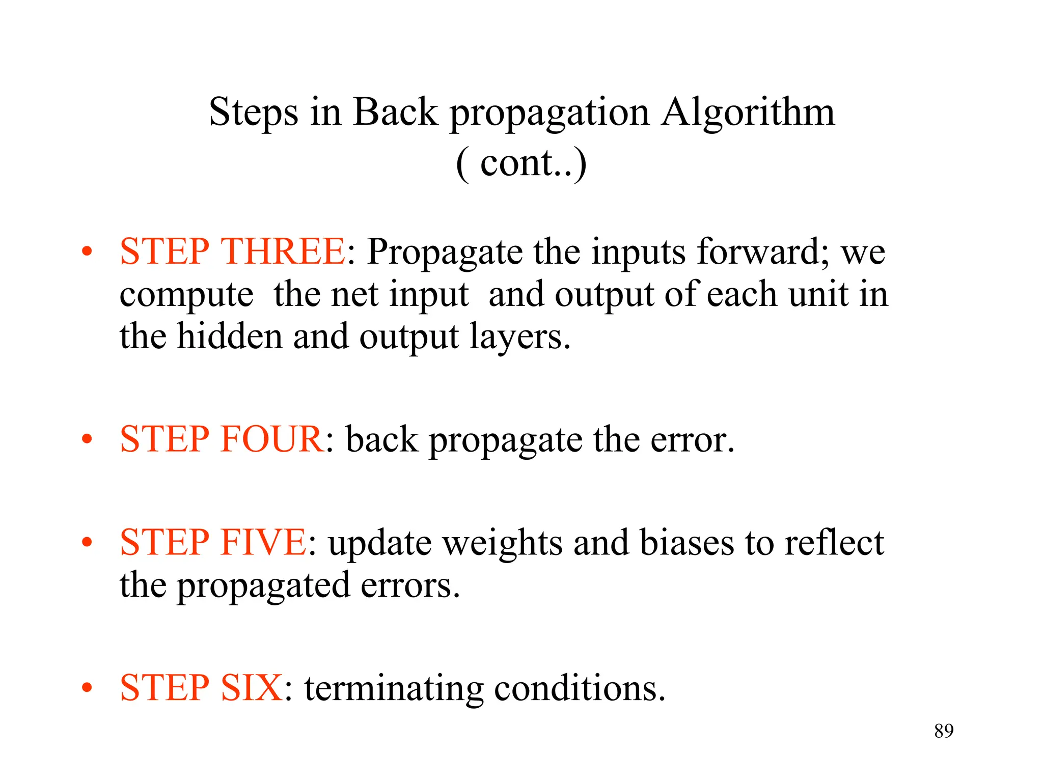
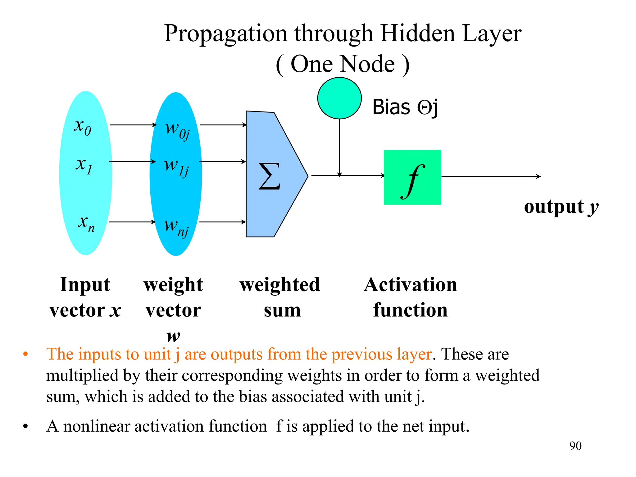
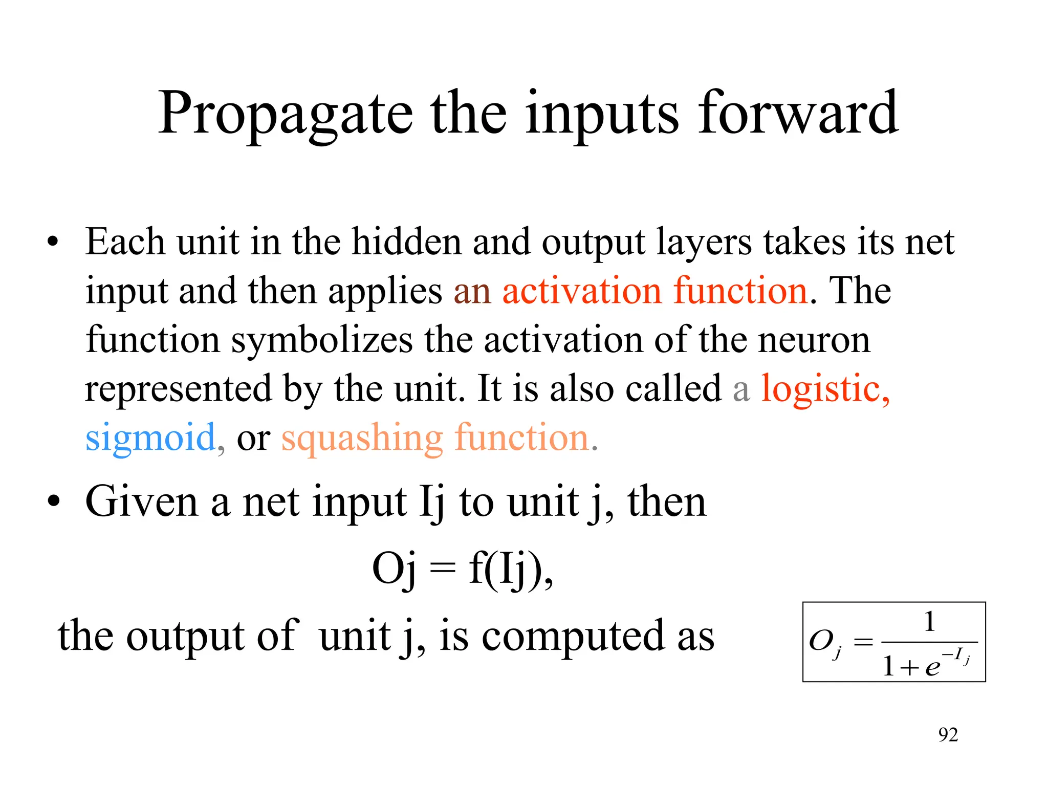
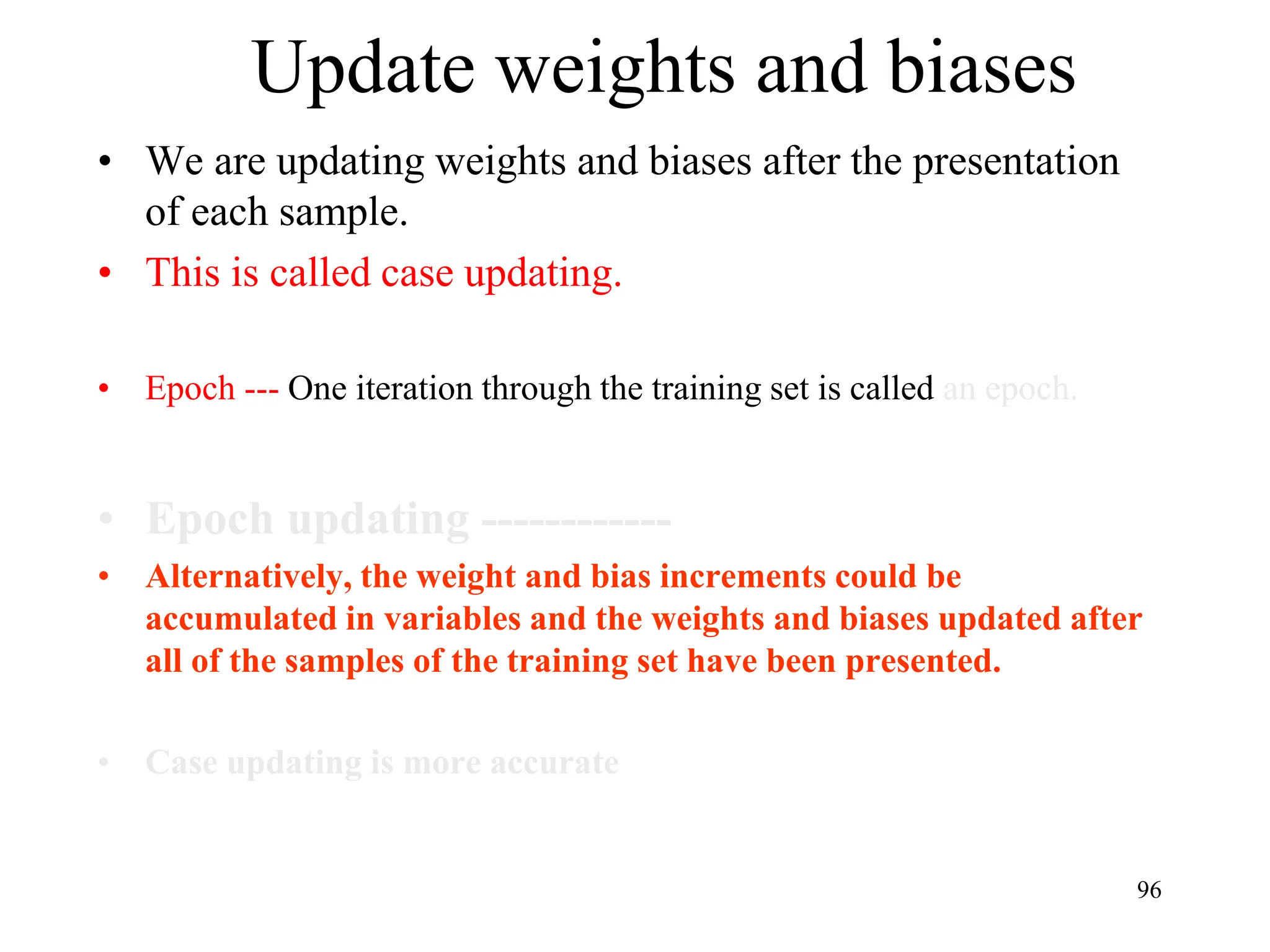
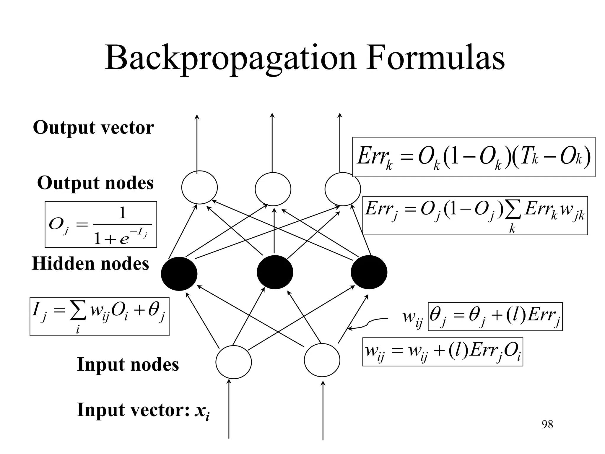
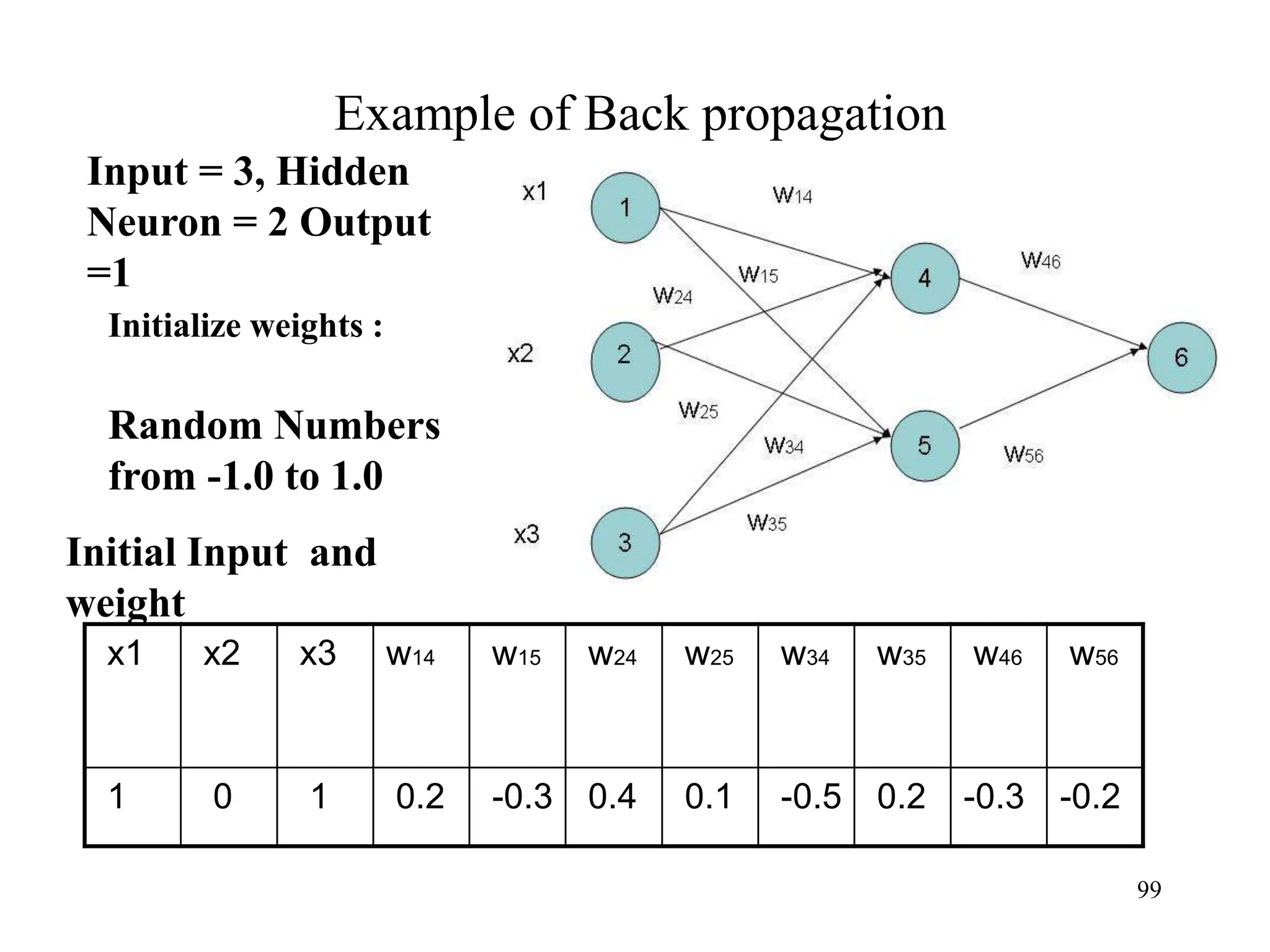
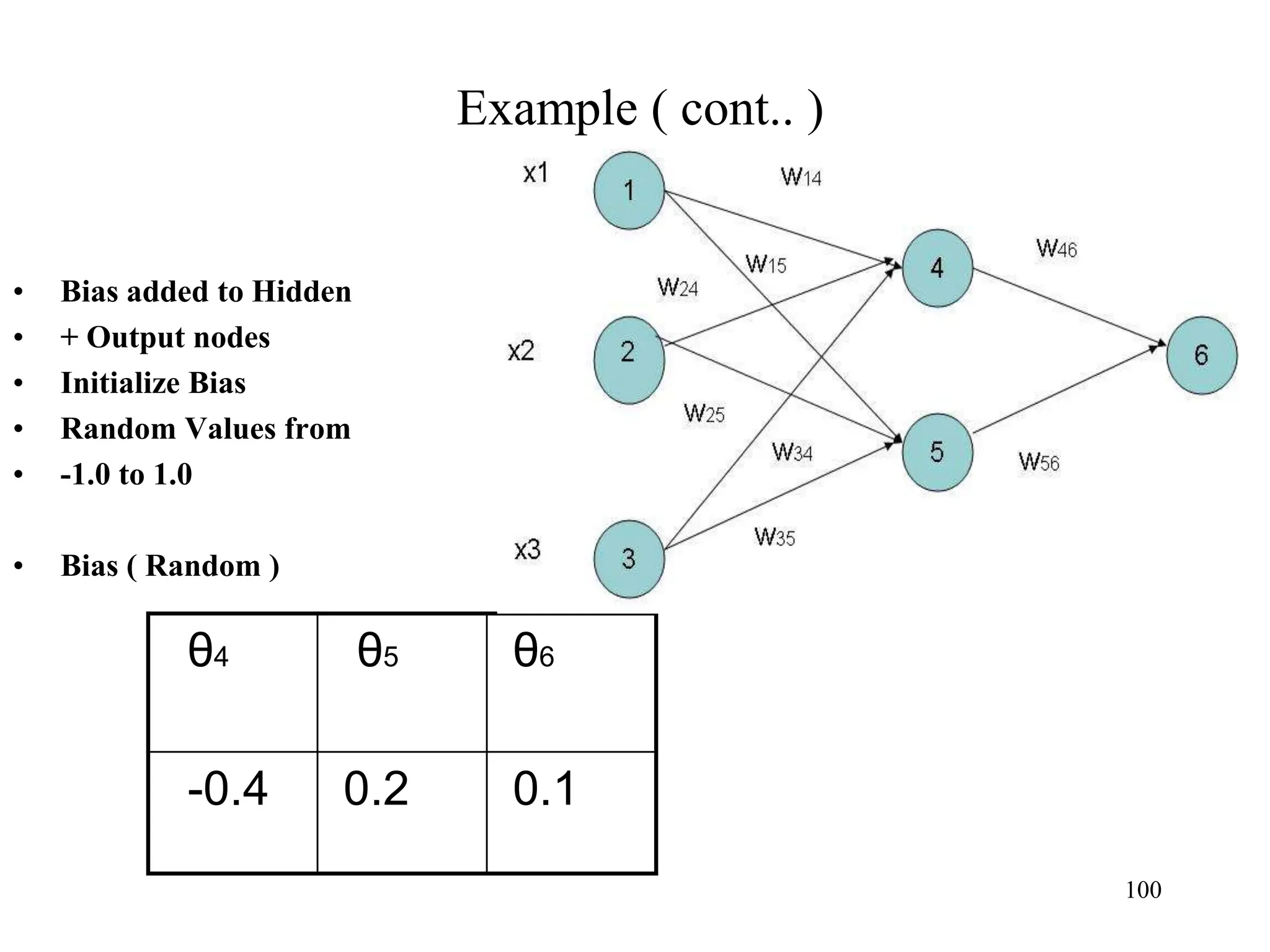
![Steps in Back propagation
Algorithm
• STEP ONE: initialize the weights and biases.
• The weights in the network are initialized to random
numbers from the interval [-1,1].
• Each unit has a BIAS associated with it
• The biases are similarly initialized to random
numbers from the interval [-1,1].
• STEP TWO: feed the training sample.
88](https://image.slidesharecdn.com/2-240709112016-70c3d429/85/Machine-learning-and-deep-learning-algorithms-88-320.jpg)


![BAYESIAN THEOREM
• A special case of Bayesian
Theorem:
P(A∩B) = P(B) x P(A|B)
P(B∩A) = P(A) x P(B|A)
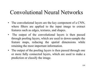
Since P(A∩B) = P(B∩A),
P(B) x P(A|B) = P(A) x P(B|A)
=> P(A|B) = [P(A) x P(B|A)] /
P(B)
A
B
P
A
P
A
B
P
A
P
A
B
P
A
P
B
P
A
B
P
A
P
B
A
P
|
|
)
|
(
)
(
)
(
)
|
(
)
(
)
|
(
A B
45](https://image.slidesharecdn.com/2-240709112016-70c3d429/75/Machine-learning-and-deep-learning-algorithms-45-2048.jpg)


![NAÏVE BAYES CLASSIFIER
Abstractly, probability model for a classifier is a
conditional model
P(C|F1,F2,…,Fn)
Over a dependent class variable C with a small
number of outcome or classes conditional over
several feature variables F1,…,Fn.
Naïve Bayes Formula:
P(C|F1,F2,…,Fn) = argmaxc [P(C) x P(F1|C) x P(F2|C)
x…x P(Fn|C)] / P(F1,F2,…,Fn)
Since P(F1,F2,…,Fn) is common to all probabilities, we
need not evaluate the denominator for comparisons.
50](https://image.slidesharecdn.com/2-240709112016-70c3d429/75/Machine-learning-and-deep-learning-algorithms-50-2048.jpg)
![NAÏVE BAYES CLASSIFIER
P(yes)xP(sunny|yes)xP(cool|yes)xP(high|yes) x
P(strong|yes) = 0.0053
P(no)xP(sunny|no)xP(cool|no)xP(high|no) x
P(strong|no) = 0.0206
So the class for this instance is ‘no’. We can
normalize the probility by:
[0.0206]/[0.0206+0.0053] = 0.795
54](https://image.slidesharecdn.com/2-240709112016-70c3d429/75/Machine-learning-and-deep-learning-algorithms-54-2048.jpg)
![NAÏVE BAYES CLASSIFIER
M-Estimate Formula:
[c + k] / [n + m] where c/n is the original
probability used before, k=1 and
m= equivalent sample size.
Using this method our new values of
probability is given below-
57](https://image.slidesharecdn.com/2-240709112016-70c3d429/75/Machine-learning-and-deep-learning-algorithms-57-2048.jpg)


![Neural Network Classifier
• Input: Classification data
It contains classification attribute
• Data is divided, as in any classification problem.
[Training data and Testing data]
• All data must be normalized.
(i.e. all values of attributes in the database are changed to contain values
in the internal [0,1] or[-1,1])
Neural Network can work with data in the range of (0,1) or (-1,1)
77](https://image.slidesharecdn.com/2-240709112016-70c3d429/75/Machine-learning-and-deep-learning-algorithms-77-2048.jpg)

![Steps in Back propagation
Algorithm
• STEP ONE: initialize the weights and biases.
• The weights in the network are initialized to random
numbers from the interval [-1,1].
• Each unit has a BIAS associated with it
• The biases are similarly initialized to random
numbers from the interval [-1,1].
• STEP TWO: feed the training sample.
88](https://image.slidesharecdn.com/2-240709112016-70c3d429/75/Machine-learning-and-deep-learning-algorithms-88-2048.jpg)


![Agentic Systems and Compliance - A brief intro [1.2]](https://cdn.slidesharecdn.com/ss_thumbnails/agenticsystemsandcompliace-1-251018025303-958a42ec-thumbnail.jpg?width=600ounds&width=560&fit=bounds)