Table of Content
Introduction
What Is MS Excel?
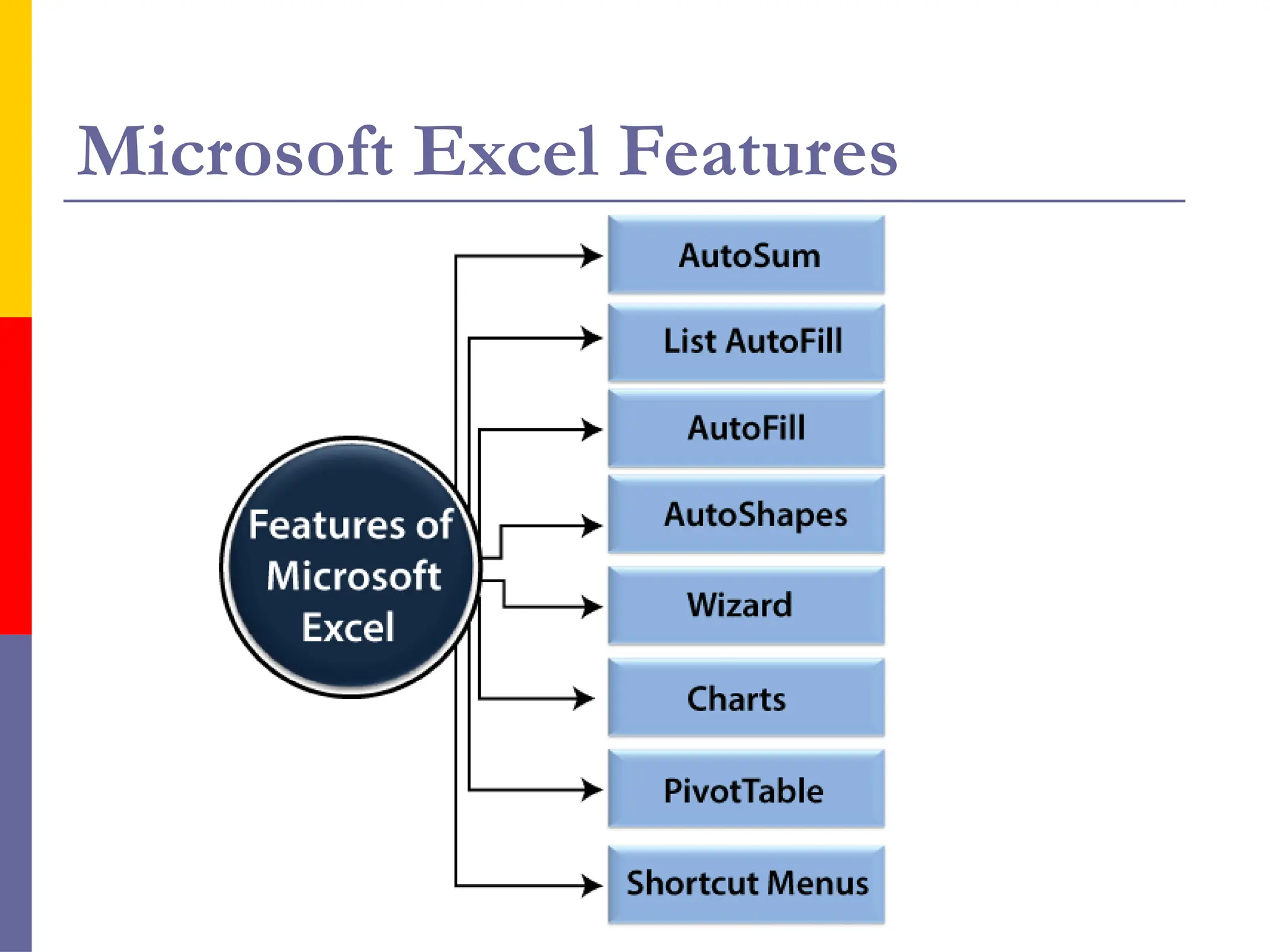
Microsoft Excel Features
Why Use Excel?
Explanation of key terms in MS Excel
Navigation of Excel Window and Basic Tools
Creation of a Workbook
Workbook - Data Entry, Formatting
Calculations: total, average, simple formula
3.
MS Excel Introduction
Microsoft Excel is a computer
application program written by
Microsoft. It mainly comprises
tabs, groups of commands, and
worksheets. It stores the data in
tabular form and allows the users
to perform operations on them.
4.
What is MicrosoftExcel?
Microsoft Excel is an office use application designed
by Microsoft. It comes with Office Suite with
several other Microsoft applications, such as Word,
Powerpoint, Access, Outlook, and OneNote, etc. It is
supported in Windows as well as Mac operating
system too.
Why Use Excel?
It is the most popular spreadsheet program in the
world
It is easy to learn and to get started.
The skill ceiling is high, which means that you can do
more advanced things as you become better
It can be used with both work and in everyday life,
such as to create a family budget
It has a huge community support
It is continuously supported by Microsoft
7.
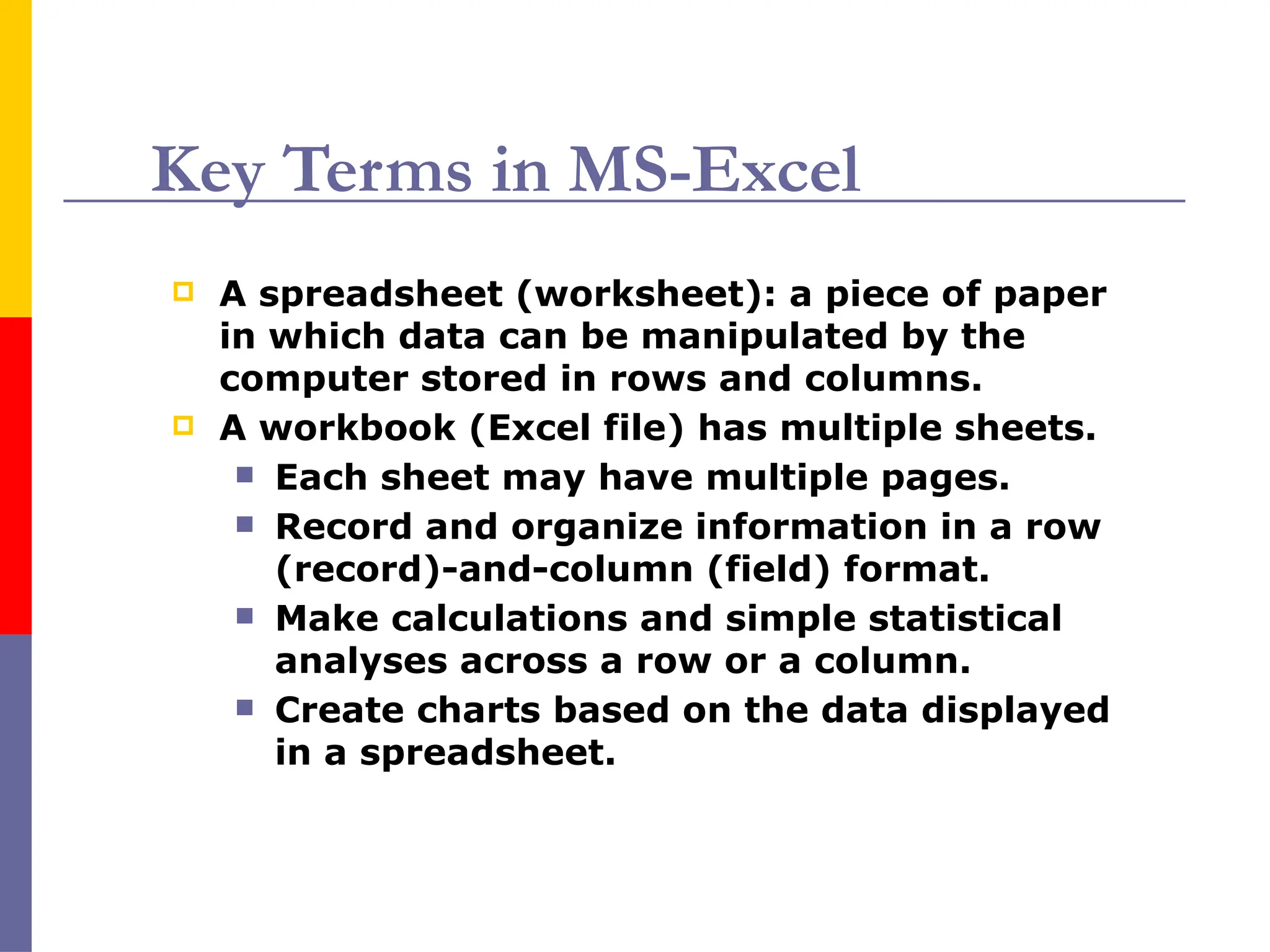
Key Terms inMS-Excel
A spreadsheet (worksheet): a piece of paper
in which data can be manipulated by the
computer stored in rows and columns.
A workbook (Excel file) has multiple sheets.
Each sheet may have multiple pages.
Record and organize information in a row
(record)-and-column (field) format.
Make calculations and simple statistical
analyses across a row or a column.
Create charts based on the data displayed
in a spreadsheet.
8.
Workbook vs Sheets
A workbook refers to an Excel document. You will
sometimes hear it called a “spreadsheet.”
In Default, each workbook has “Sheet1”, You can
rename these sheets to something more fitting to
your purpose(e.g. Fall Term, Summer Term,
Spring Term…)
You can add sheets if you’d like to.
Your workbook is the ENTIRE file and the file
name should reflect the function the file serves.
Friends_Address.xlsx
Inventory.xlsx
9.
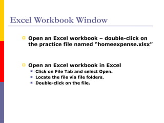
Excel Workbook Window
Open an Excel workbook – double-click on
the practice file named “homeexpense.xlsx”
Open an Excel workbook in Excel
Click on File Tab and select Open.
Locate the file via file folders.
Double-click on the file.
10.
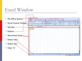
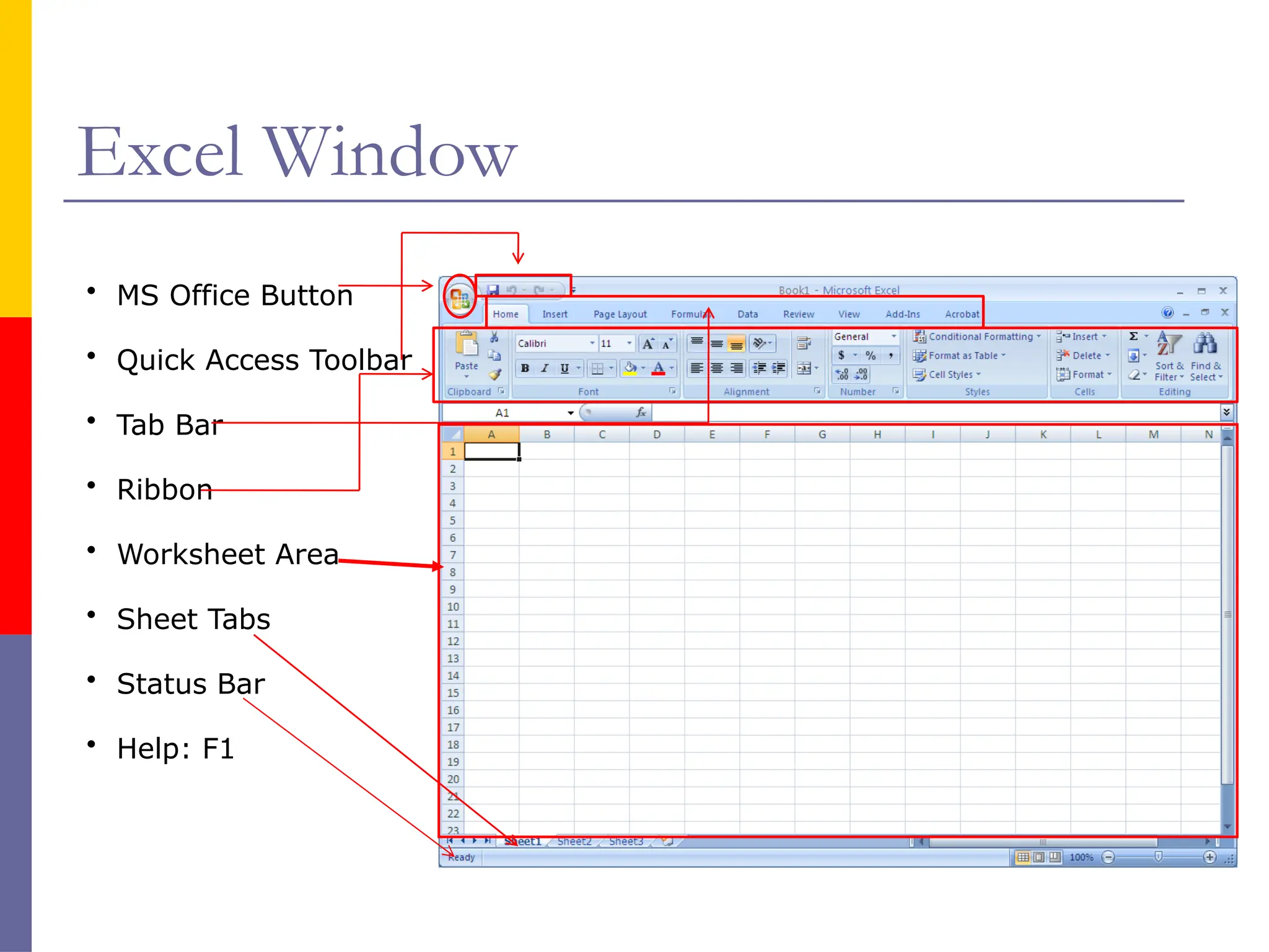
Excel Window
• MSOffice Button
• Quick Access Toolbar
• Tab Bar
• Ribbon
• Worksheet Area
• Sheet Tabs
• Status Bar
• Help: F1
11.
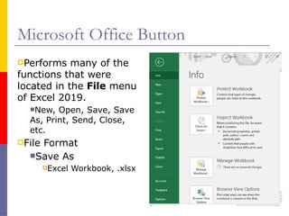
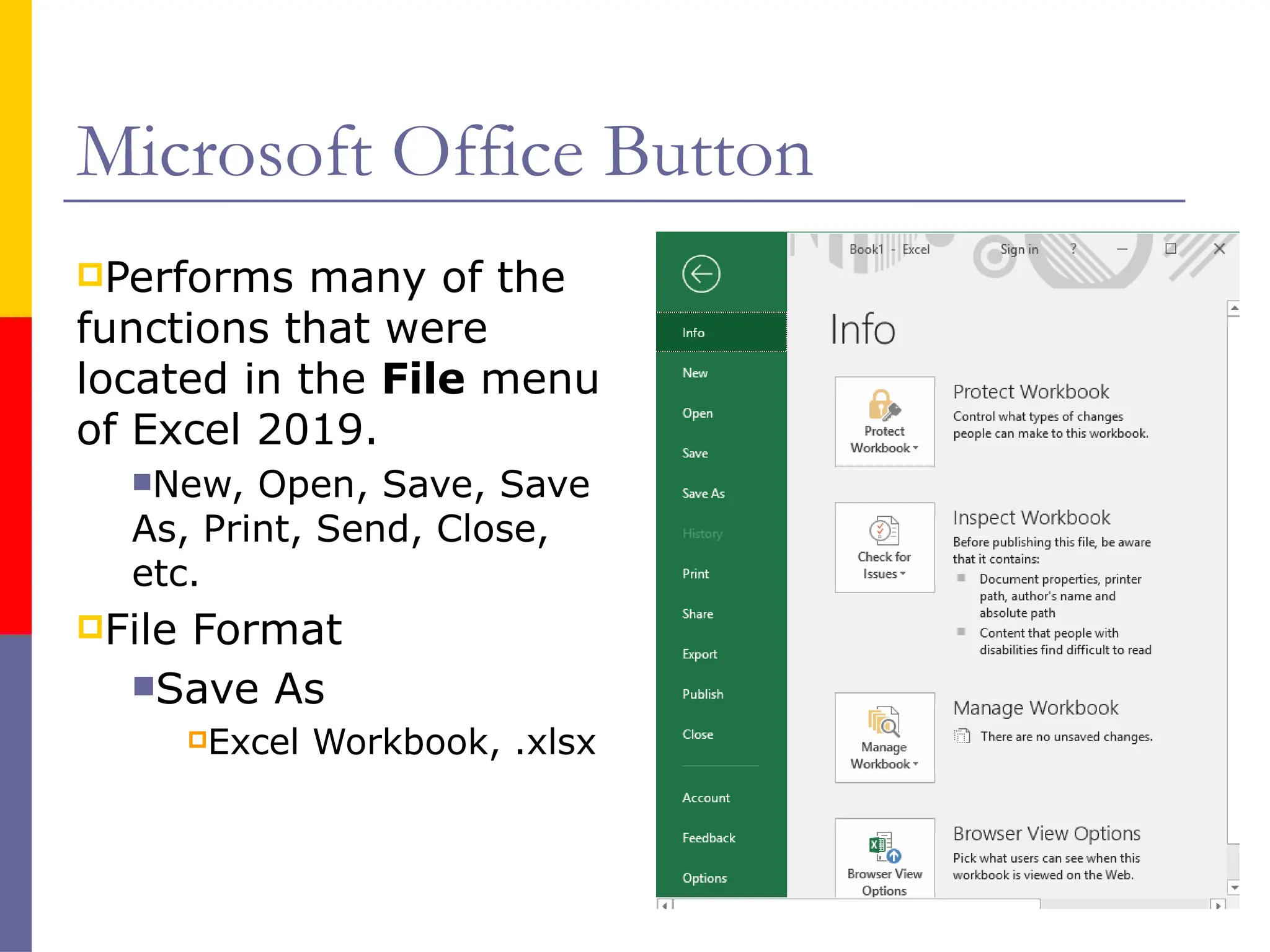
Microsoft Office Button
Performsmany of the
functions that were
located in the File menu
of Excel 2019.
New, Open, Save, Save
As, Print, Send, Close,
etc.
File Format
Save As
Excel Workbook, .xlsx
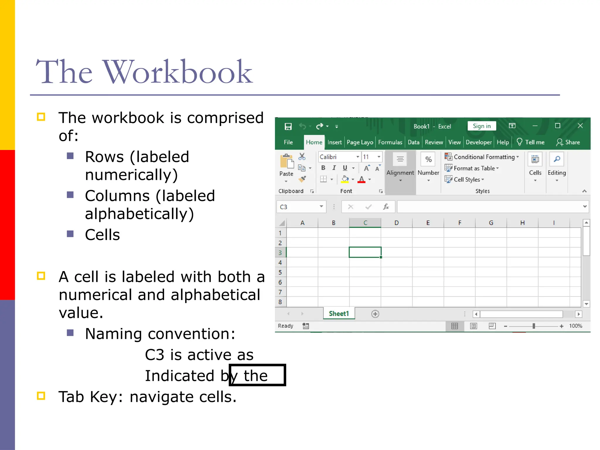
The Workbook
Theworkbook is comprised
of:
Rows (labeled
numerically)
Columns (labeled
alphabetically)
Cells
A cell is labeled with both a
numerical and alphabetical
value.
Naming convention:
C3 is active as
Indicated by the
Tab Key: navigate cells.
14.
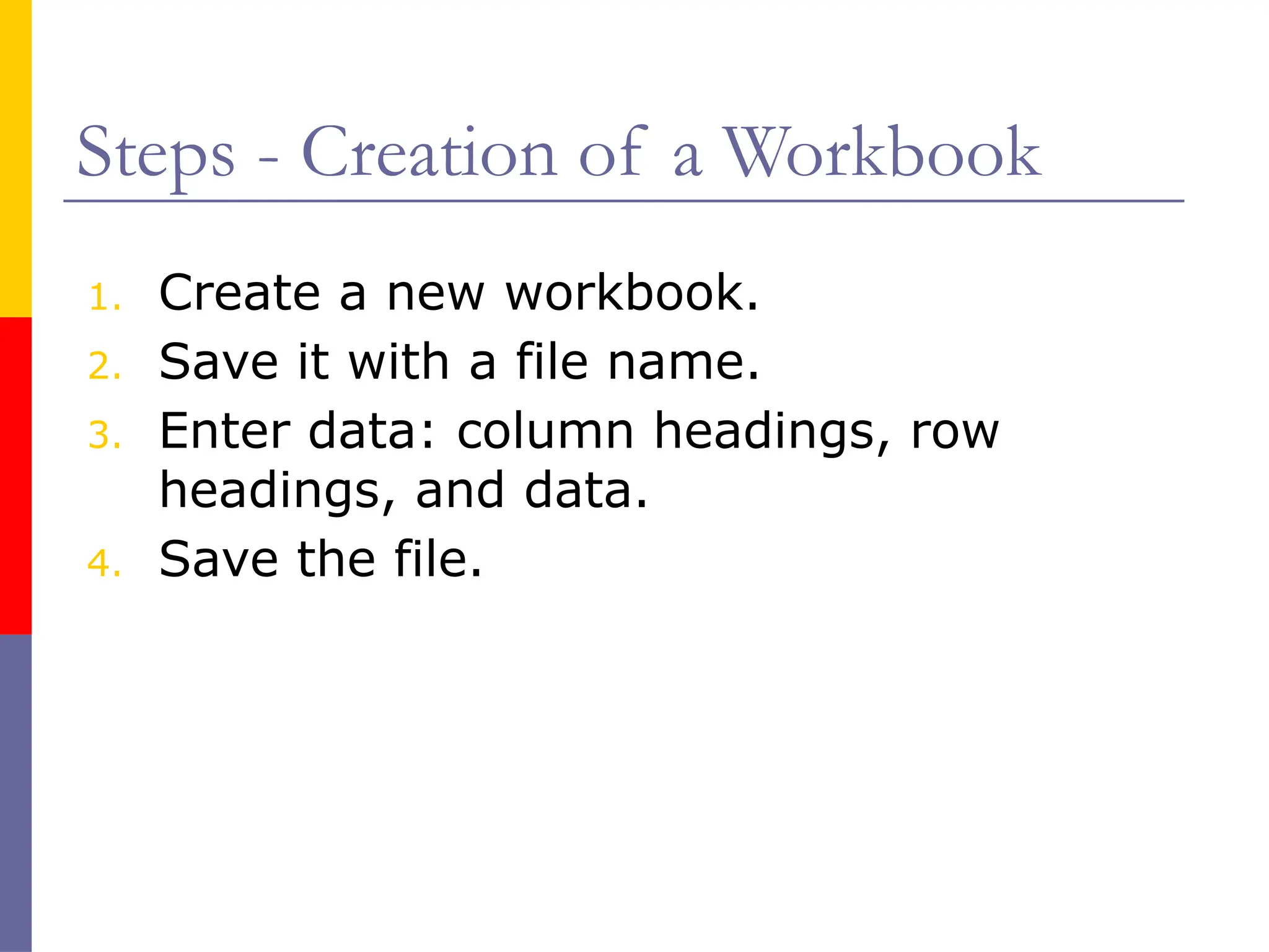
Steps - Creationof a Workbook
1. Create a new workbook.
2. Save it with a file name.
3. Enter data: column headings, row
headings, and data.
4. Save the file.
15.
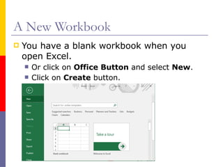
A New Workbook
You have a blank workbook when you
open Excel.
Or click on Office Button and select New.
Click on Create button.
16.
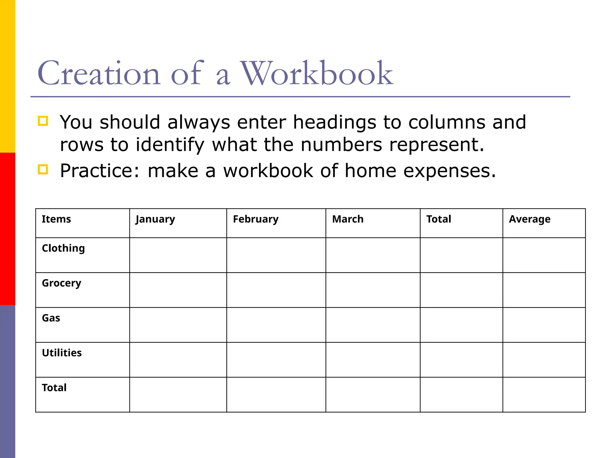
Creation of aWorkbook
You should always enter headings to columns and
rows to identify what the numbers represent.
Practice: make a workbook of home expenses.
Items January February March Total Average
Clothing
Grocery
Gas
Utilities
Total
17.
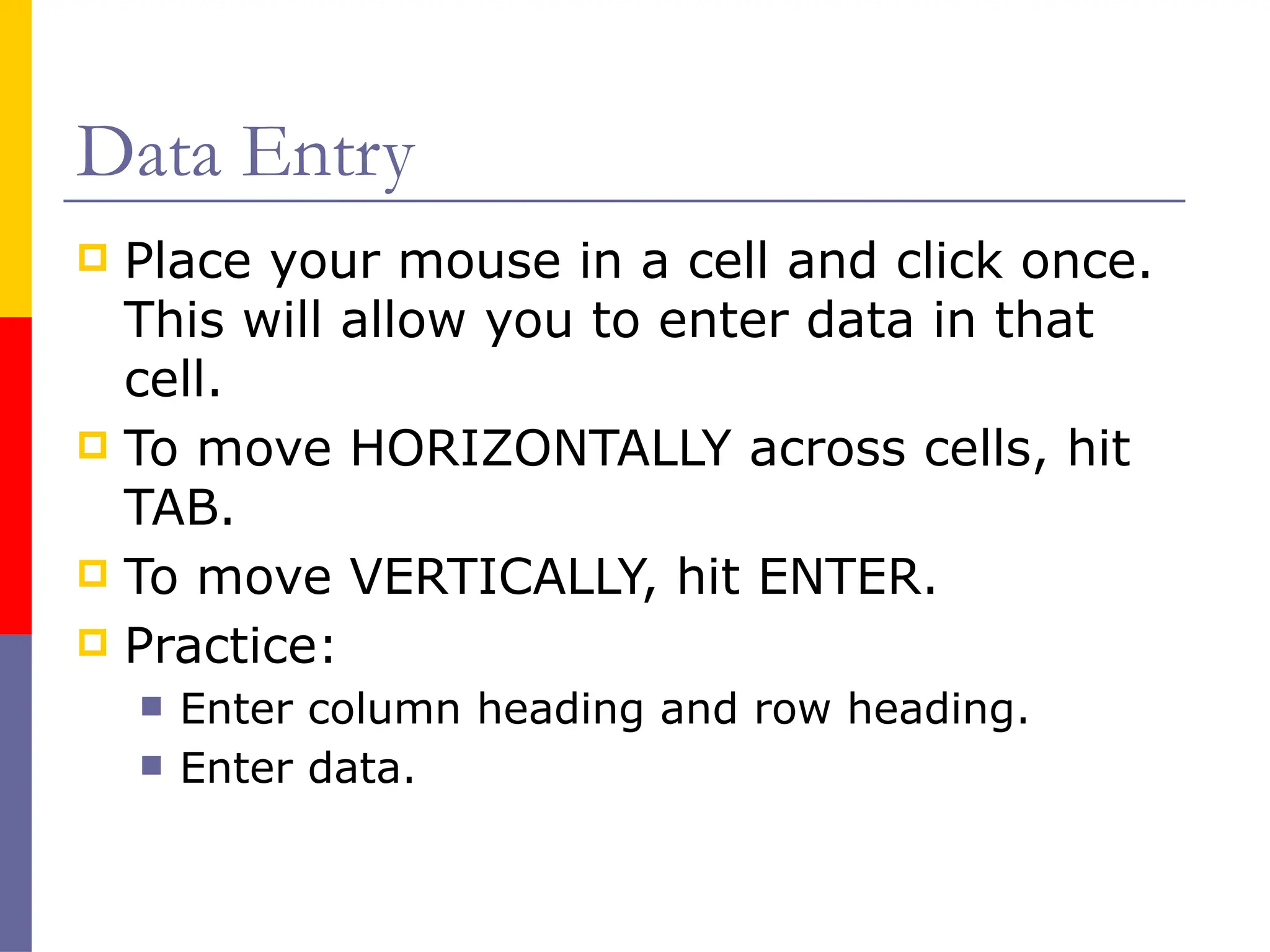
Data Entry
Placeyour mouse in a cell and click once.
This will allow you to enter data in that
cell.
To move HORIZONTALLY across cells, hit
TAB.
To move VERTICALLY, hit ENTER.
Practice:
Enter column heading and row heading.
Enter data.
18.
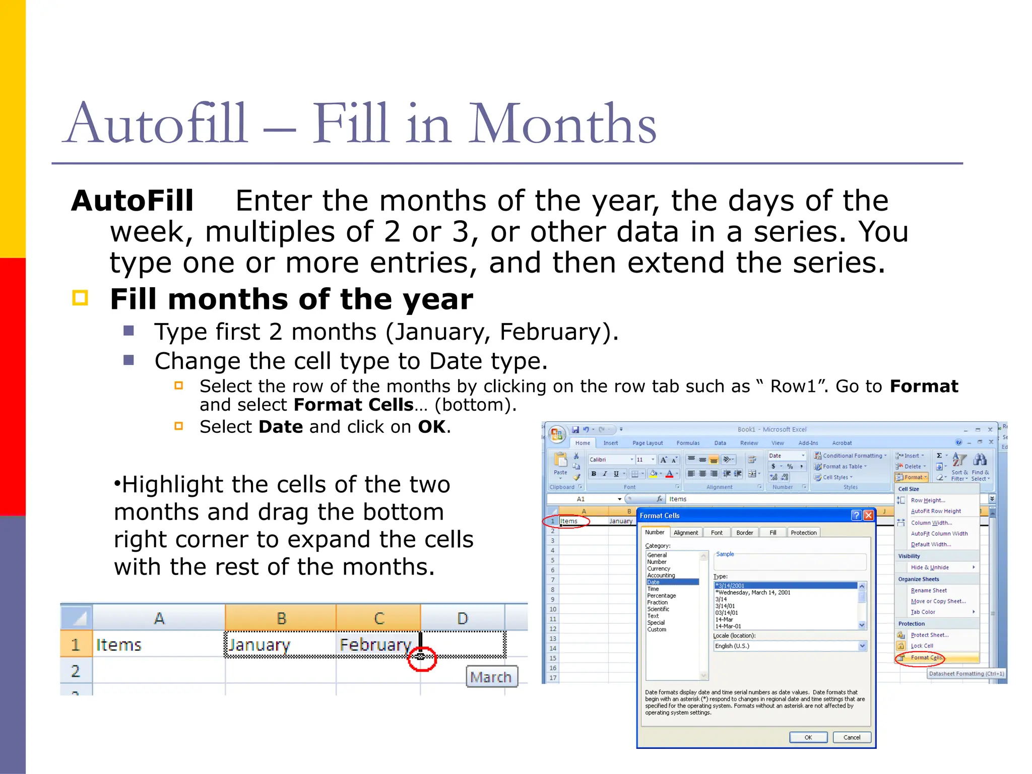
Autofill – Fillin Months
AutoFill Enter the months of the year, the days of the
week, multiples of 2 or 3, or other data in a series. You
type one or more entries, and then extend the series.
Fill months of the year
Type first 2 months (January, February).
Change the cell type to Date type.
Select the row of the months by clicking on the row tab such as “ Row1”. Go to Format
and select Format Cells… (bottom).
Select Date and click on OK.
•Highlight the cells of the two
months and drag the bottom
right corner to expand the cells
with the rest of the months.
19.
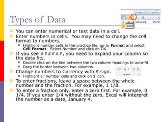
Types of Data
You can enter numerical or text data in a cell.
Enter numbers in cells. You may need to change the cell
format to numbers.
Highlight number cells in the practice file, go to Format and select
Cell Format. Select Number and click on OK.
If you see ######, you need to expand your column so
the data fits.
Double click on the line between the two column headings to auto-fit.
Drag the border between two columns.
Change numbers to Currency with $ sign.
Highlight all number cells and click on $ icon.
To enter fractions, leave a space between the whole
number and the fraction. For example, 1 1/8.
To enter a fraction only, enter a zero first. For example, 0
1/4. If you enter 1/4 without the zero, Excel will interpret
the number as a date, January 4.
20.
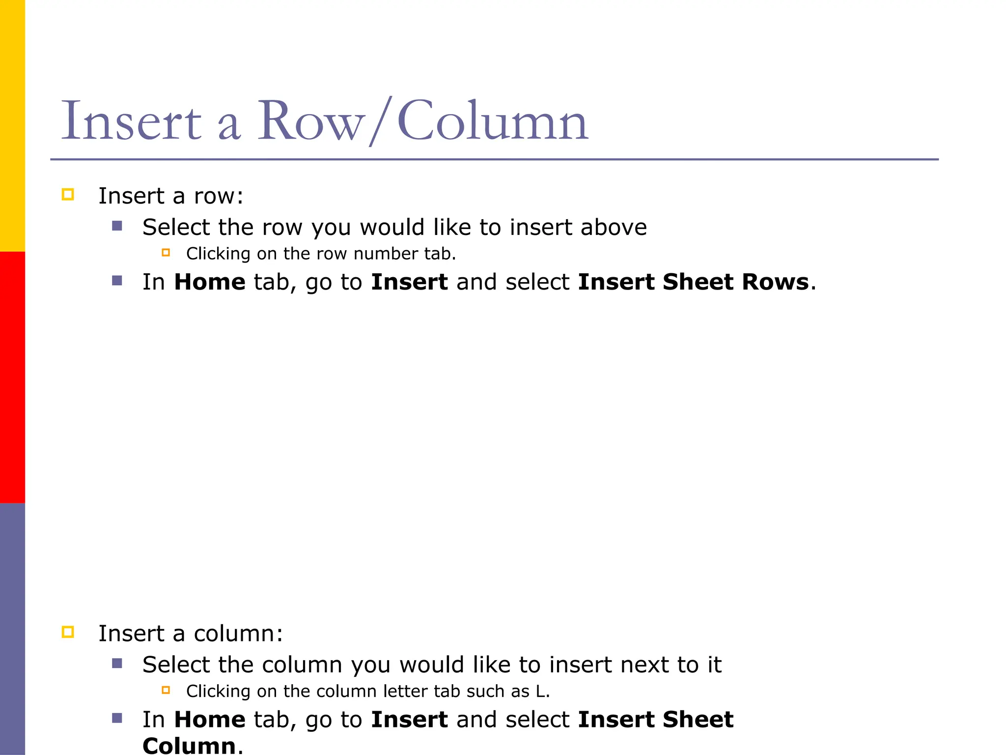
Insert a Row/Column
Insert a row:
Select the row you would like to insert above
Clicking on the row number tab.
In Home tab, go to Insert and select Insert Sheet Rows.
Insert a column:
Select the column you would like to insert next to it
Clicking on the column letter tab such as L.
In Home tab, go to Insert and select Insert Sheet
Column.
21.
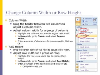
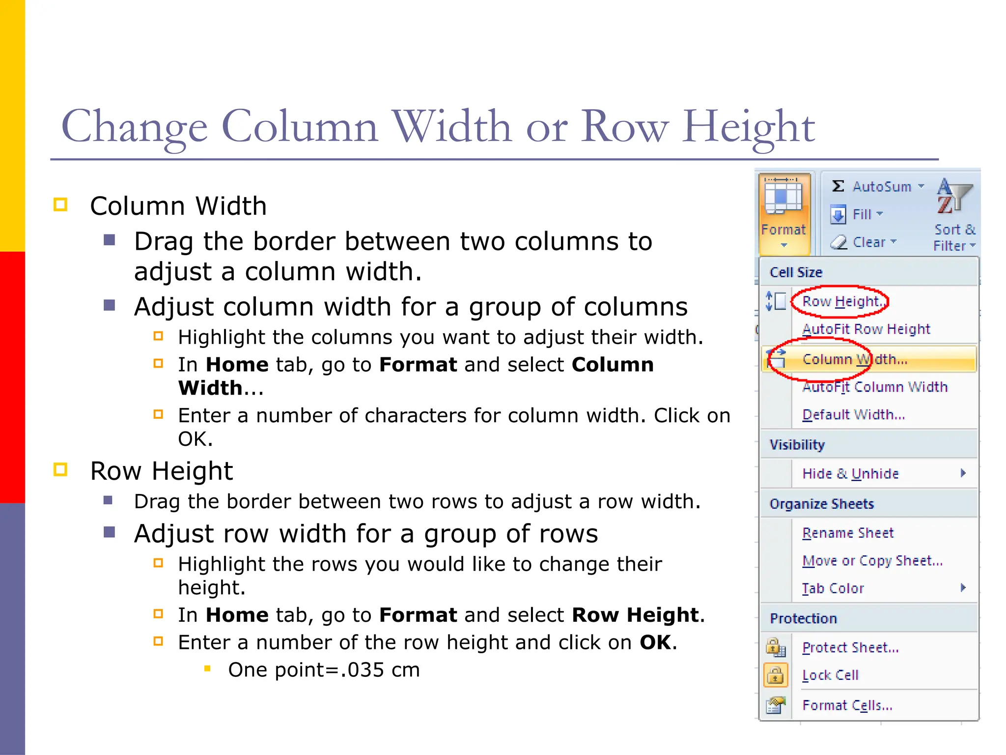
Change Column Widthor Row Height
Column Width
Drag the border between two columns to
adjust a column width.
Adjust column width for a group of columns
Highlight the columns you want to adjust their width.
In Home tab, go to Format and select Column
Width...
Enter a number of characters for column width. Click on
OK.
Row Height
Drag the border between two rows to adjust a row width.
Adjust row width for a group of rows
Highlight the rows you would like to change their
height.
In Home tab, go to Format and select Row Height.
Enter a number of the row height and click on OK.
One point=.035 cm
22.
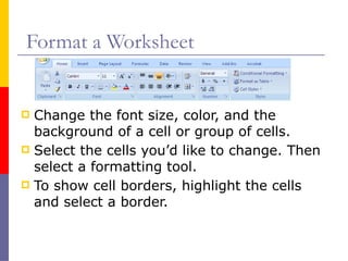
Format a Worksheet
Change the font size, color, and the
background of a cell or group of cells.
Select the cells you’d like to change. Then
select a formatting tool.
To show cell borders, highlight the cells
and select a border.
23.
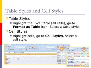
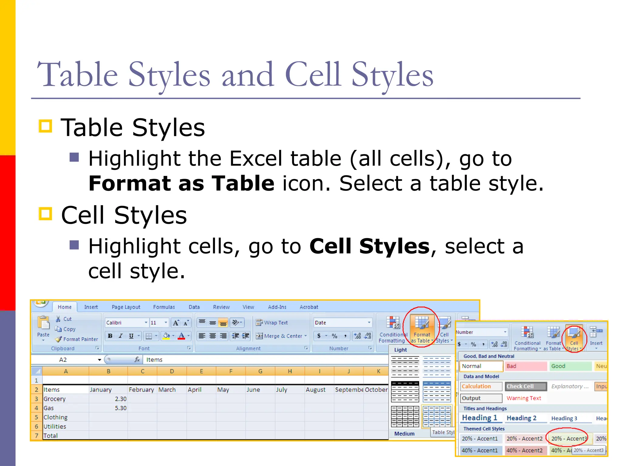
Table Styles andCell Styles
Table Styles
Highlight the Excel table (all cells), go to
Format as Table icon. Select a table style.
Cell Styles
Highlight cells, go to Cell Styles, select a
cell style.
24.
Excel - Headerand Footer
In Insert tab, click on Header & Footer icon.
Type in a header in the Header box.
Click on Go to Footer icon. Click on File Name icon to insert the file
name in the Footer box.
To go back to the Normal view of the spreadsheet, click on View tab and
select Normal.
25.
Conditional Formatting
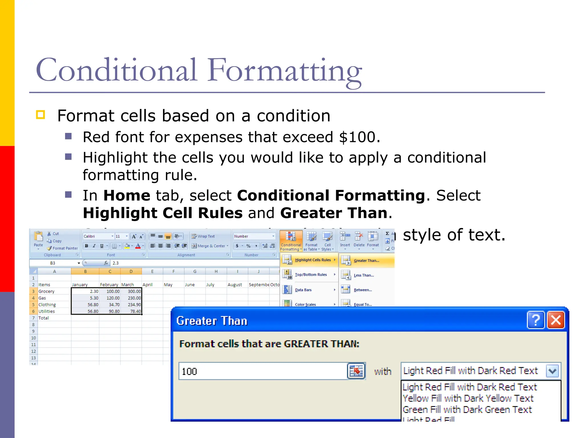
Formatcells based on a condition
Red font for expenses that exceed $100.
Highlight the cells you would like to apply a conditional
formatting rule.
In Home tab, select Conditional Formatting. Select
Highlight Cell Rules and Greater Than.
Select a cut point number (100) and a style of text.
26.
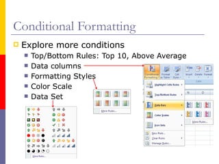
Conditional Formatting
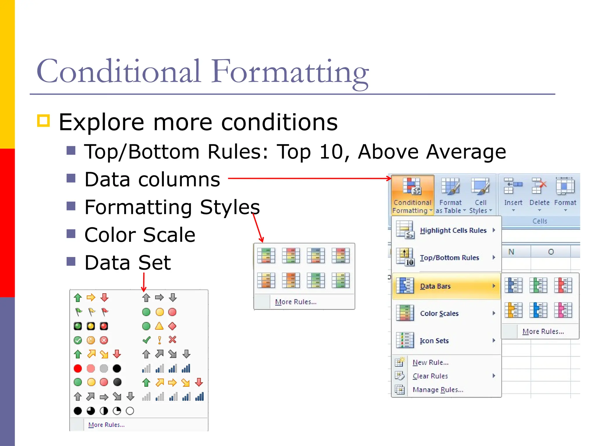
Exploremore conditions
Top/Bottom Rules: Top 10, Above Average
Data columns
Formatting Styles
Color Scale
Data Set
27.
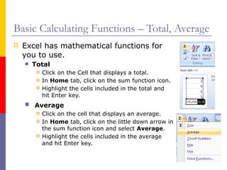
Basic Calculating Functions– Total, Average
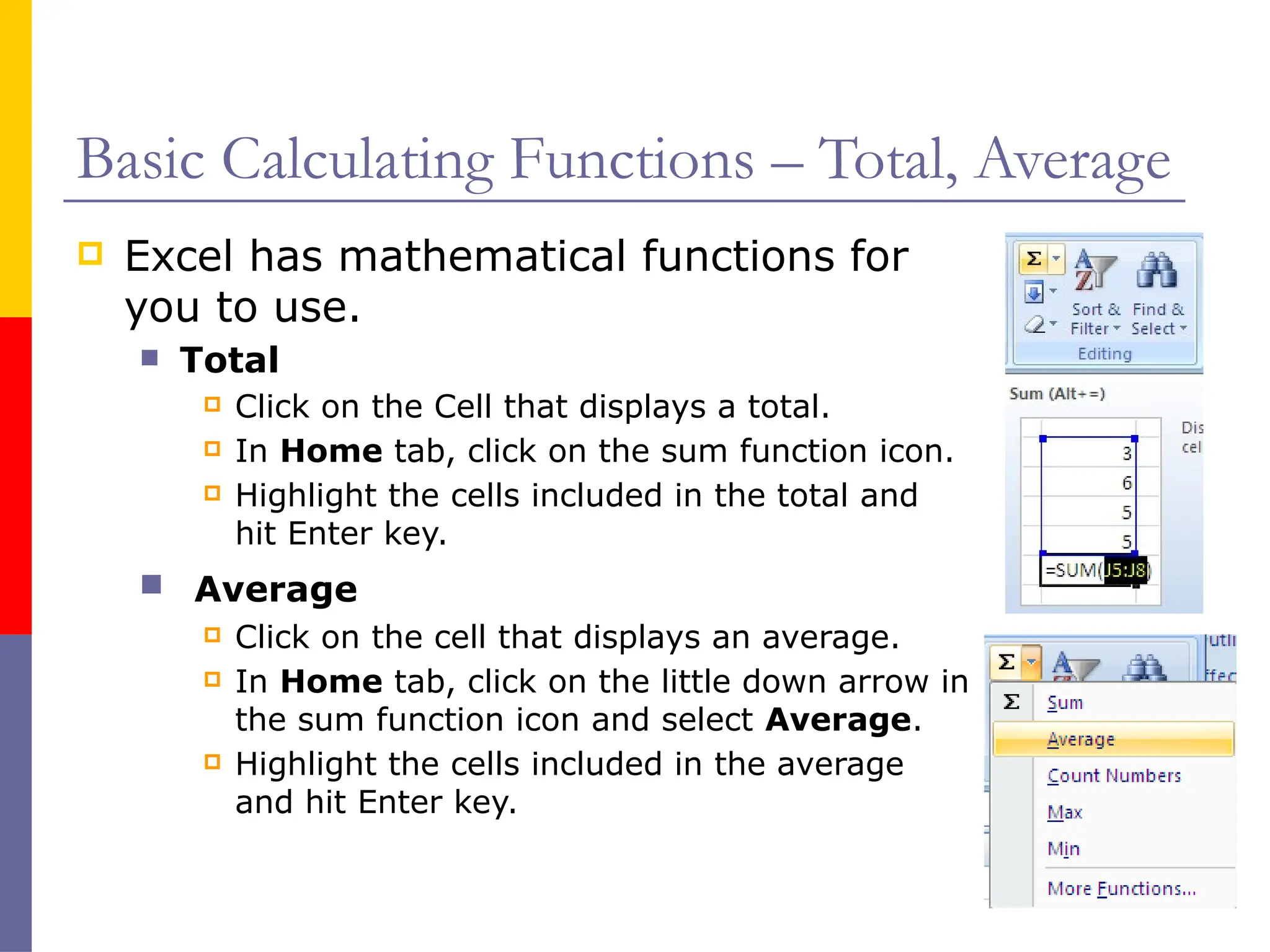
Excel has mathematical functions for
you to use.
Total
Click on the Cell that displays a total.
In Home tab, click on the sum function icon.
Highlight the cells included in the total and
hit Enter key.
Average
Click on the cell that displays an average.
In Home tab, click on the little down arrow in
the sum function icon and select Average.
Highlight the cells included in the average
and hit Enter key.
28.
Creating Basic Formula
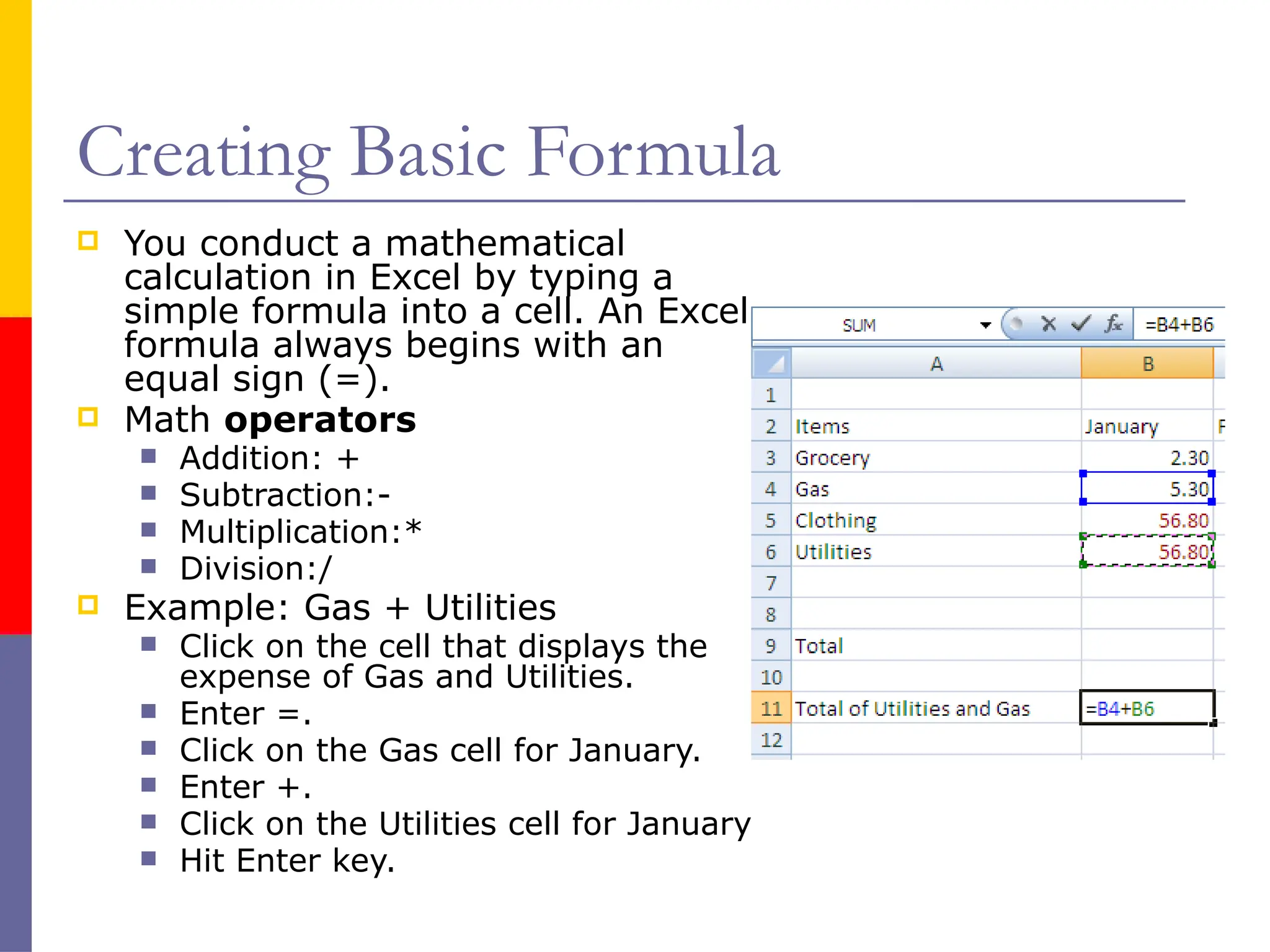
You conduct a mathematical
calculation in Excel by typing a
simple formula into a cell. An Excel
formula always begins with an
equal sign (=).
Math operators
Addition: +
Subtraction:-
Multiplication:*
Division:/
Example: Gas + Utilities
Click on the cell that displays the
expense of Gas and Utilities.
Enter =.
Click on the Gas cell for January.
Enter +.
Click on the Utilities cell for January
Hit Enter key.
29.
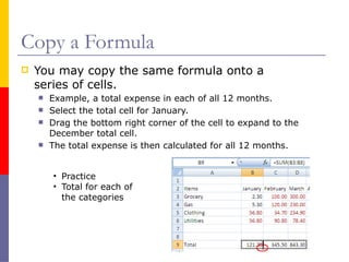
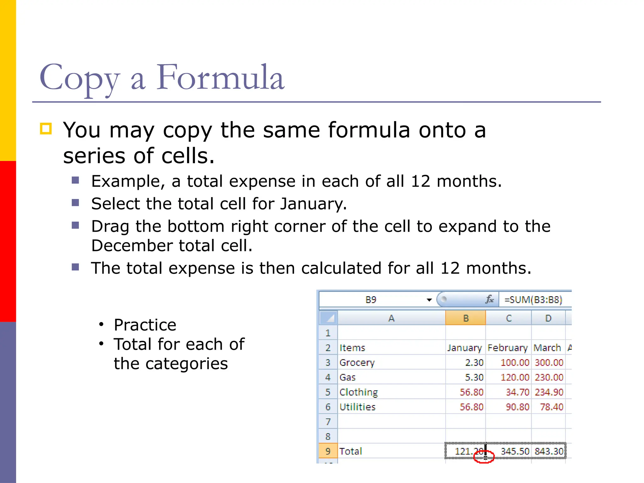
Copy a Formula
You may copy the same formula onto a
series of cells.
Example, a total expense in each of all 12 months.
Select the total cell for January.
Drag the bottom right corner of the cell to expand to the
December total cell.
The total expense is then calculated for all 12 months.
• Practice
• Total for each of
the categories
30.
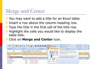
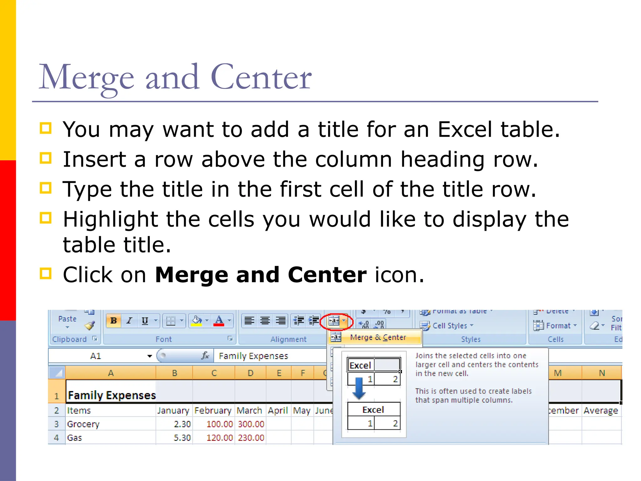
Merge and Center
You may want to add a title for an Excel table.
Insert a row above the column heading row.
Type the title in the first cell of the title row.
Highlight the cells you would like to display the
table title.
Click on Merge and Center icon.
31.
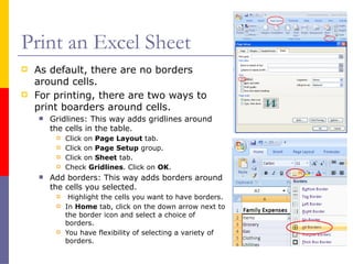
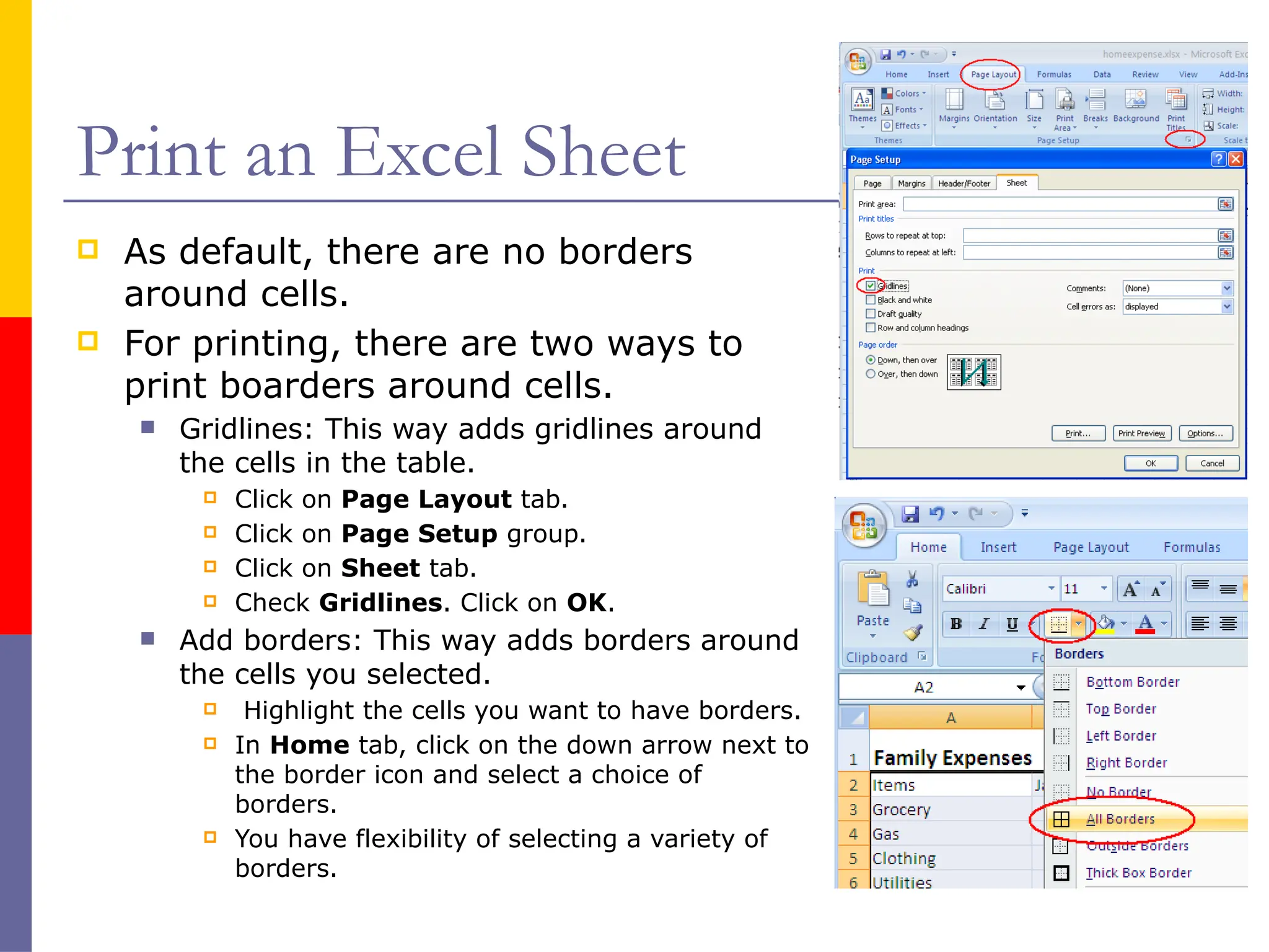
Print an ExcelSheet
As default, there are no borders
around cells.
For printing, there are two ways to
print boarders around cells.
Gridlines: This way adds gridlines around
the cells in the table.
Click on Page Layout tab.
Click on Page Setup group.
Click on Sheet tab.
Check Gridlines. Click on OK.
Add borders: This way adds borders around
the cells you selected.
Highlight the cells you want to have borders.
In Home tab, click on the down arrow next to
the border icon and select a choice of
borders.
You have flexibility of selecting a variety of
borders.
32.
Page Layout
Orientation
The vertical dotted line specifies the right border
of a page in a spreadsheet.
You may change the page orientation from
Portrait to Landscape. Go to Page Layout tab,
click on the Orientation icon and select
Landscape.
You may adjust the width of columns to fit the
columns into a page.
Double click on the border between the titles of two
columns to automatically adjust the column width.
Drag the border between the titles of two columns to
adjust the column width.
Margins
To adjust the margins of a page, in Page Layout
tab, click on Margins icon and select Custom
Margins. Change margins and click on OK.
Sheet Name
To give a name of a sheet, double-click on the
sheet tab and enter the name.
33.
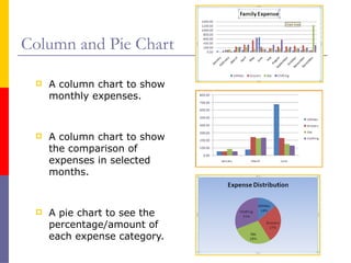
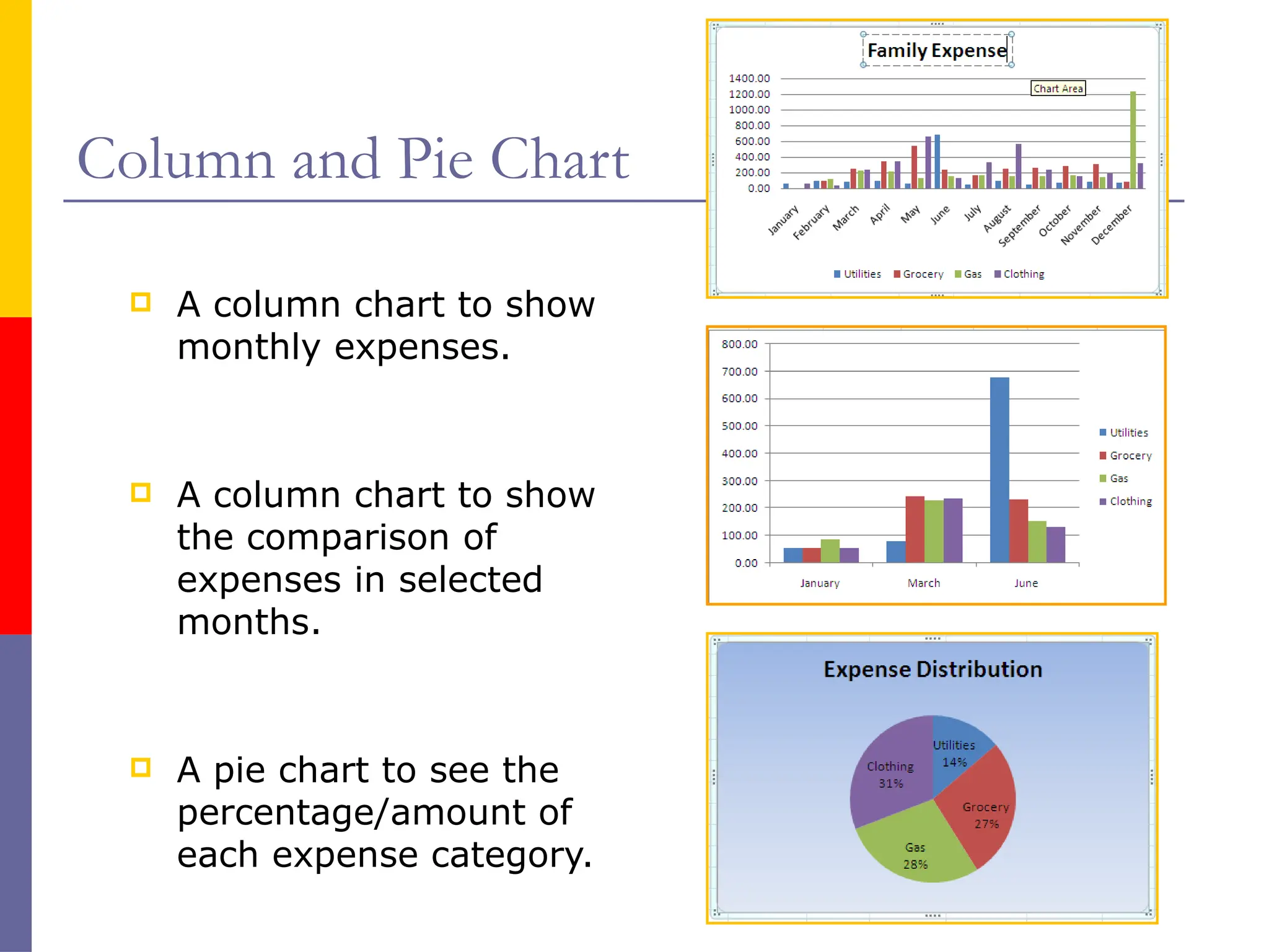
Column and PieChart
A column chart to show
monthly expenses.
A column chart to show
the comparison of
expenses in selected
months.
A pie chart to see the
percentage/amount of
each expense category.
34.
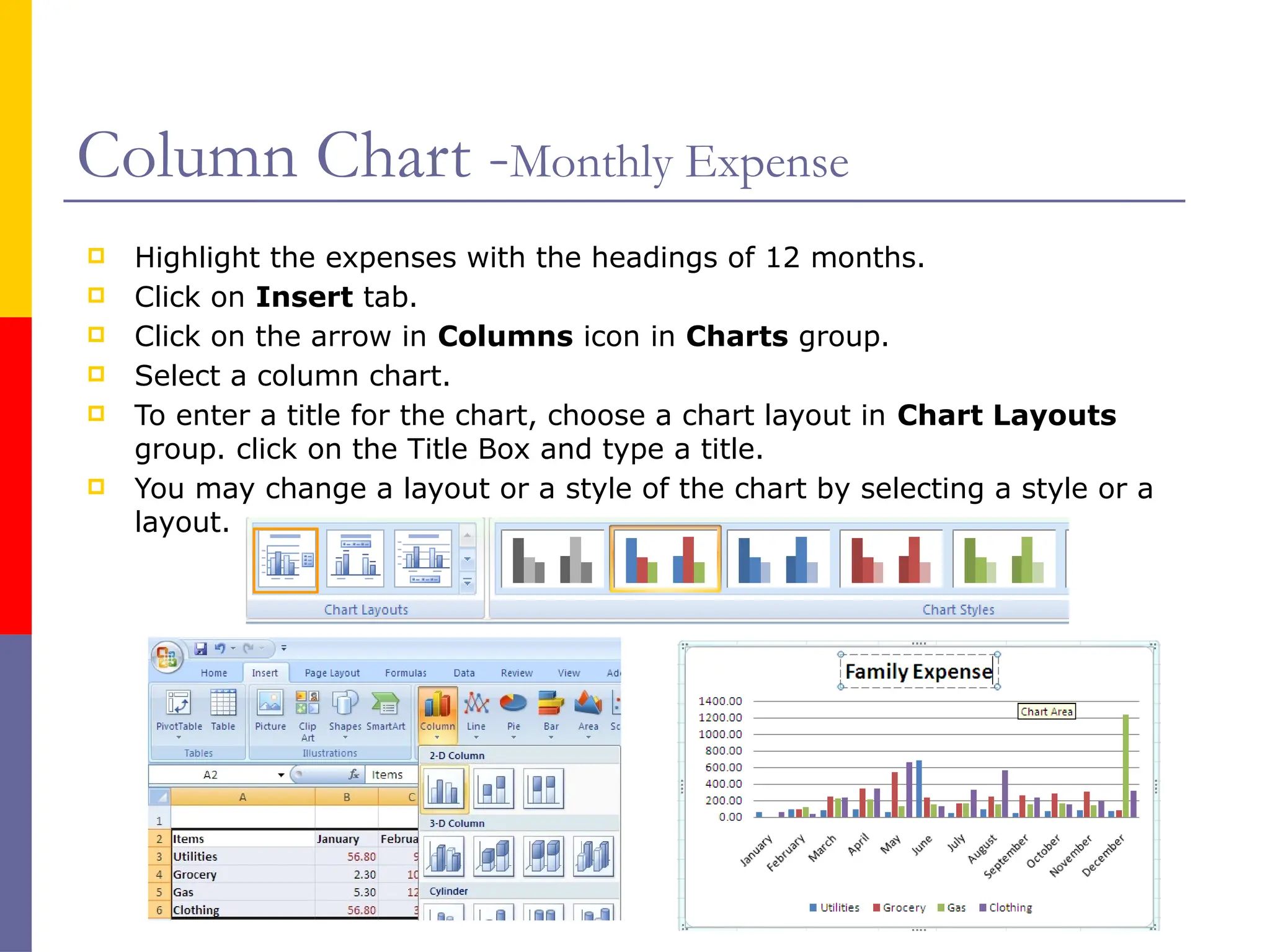
Column Chart -MonthlyExpense
Highlight the expenses with the headings of 12 months.
Click on Insert tab.
Click on the arrow in Columns icon in Charts group.
Select a column chart.
To enter a title for the chart, choose a chart layout in Chart Layouts
group. click on the Title Box and type a title.
You may change a layout or a style of the chart by selecting a style or a
layout.
35.
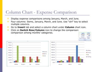
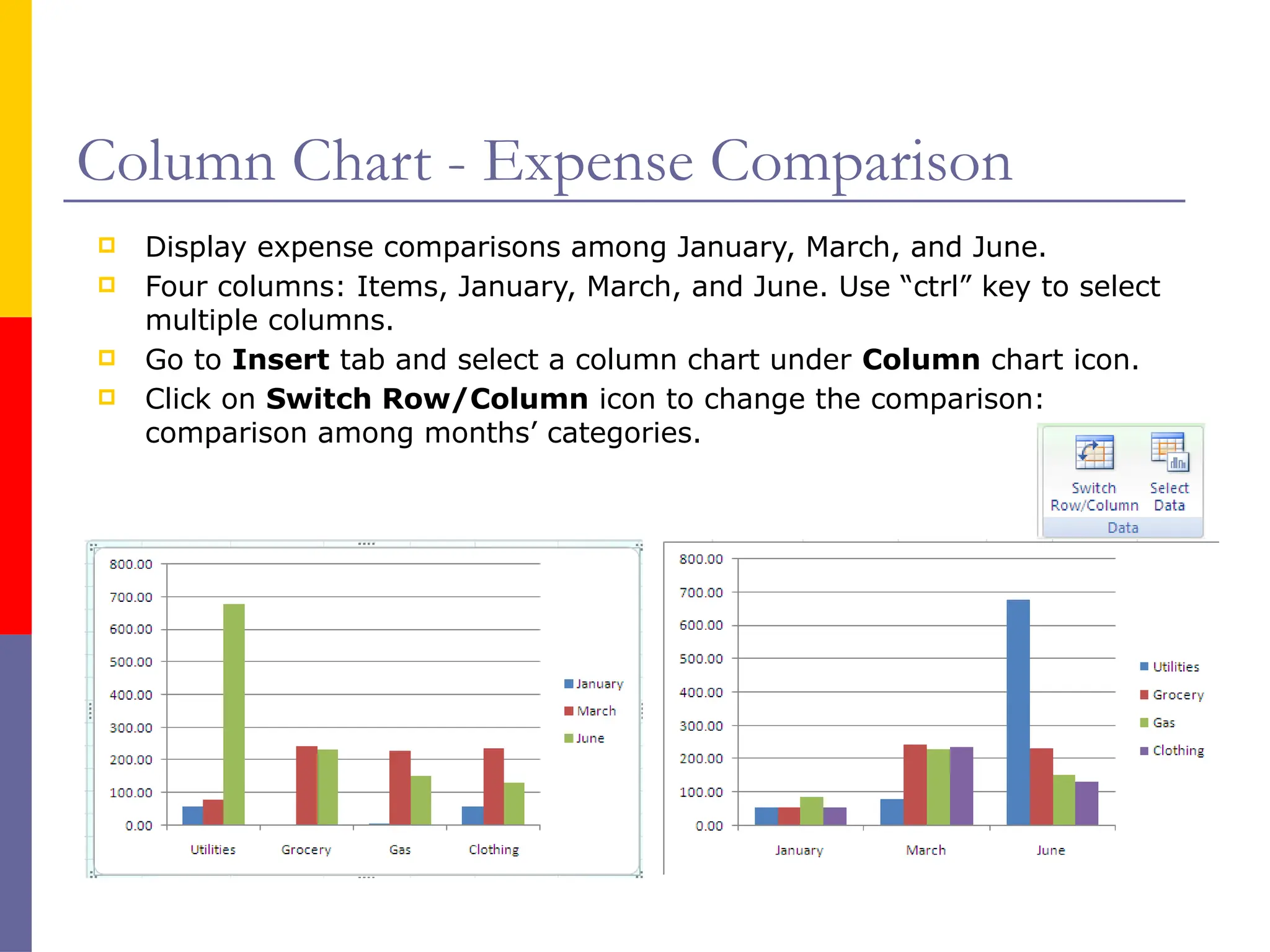
Column Chart -Expense Comparison
Display expense comparisons among January, March, and June.
Four columns: Items, January, March, and June. Use “ctrl” key to select
multiple columns.
Go to Insert tab and select a column chart under Column chart icon.
Click on Switch Row/Column icon to change the comparison:
comparison among months’ categories.
36.
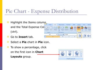
Pie Chart -Expense Distribution
Highlight the Items column
and the Total Expense Column
(ctrl).
Go to Insert tab.
Select a Pie chart in Pie icon.
To show a percentage, click
on the first icon in Chart
Layouts group.
37.
Pie Chart -Format
To add a title for the pie chart, choose a layout with a title
box, click on the title box, and type the title.
Add background for the chart: Right-click on the chart and
select Format Chart Area….
Select a Fill style, border color, border style, etc. Click on Close.
38.
Key Steps inCharting
Create the columns/rows that have the data you need
to draw a chart.
Select the columns/rows needed.
Hold “ctrl” key to select non-continuous columns.
Hold “shift” key to select continuous columns.
Select a chart type in Insert tab.
Enter Chart title.
Select a style of a chart.
#7 Excel is a spreadsheet application. With Excel, we can record information in a row-and-column format. We can make simple calculations or statistical analysis across a row or a column. Create charts on the basis of the recorded data. Records of family expenses, Travel log with calculation of the mileage and reimbursement, student grade book with calculation of the final grades and making charts.
#11 -20 minutes
Open MS Word. File/Edit Menus are grouped to Office Button.
Office Button: common commands: new, open, save, print, email, etc. Prepare-Details to describe or identify a document.
Practice: type in formation, save it as a file. open a file. Print, print-preview, send as an email attachment.
#12
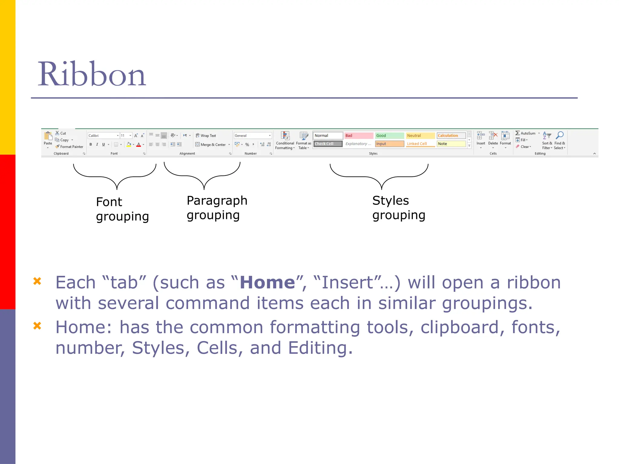
Introduced a term as Ribbon. The command icons are grouped in each of the tabs. Each tab opens a ribbon, a group of commands.
Practice: Explore the tabs with commonly used commands.
Home: formatting – font, size, bold, italic, find/replace, copy/paste
#13 The first 26 columns have the letters from A through Z. Each worksheet contains 256 columns in all, so after Z the letters begin again in pairs, AA through AZ. See Figure 2.
After AZ, the letter pairs start again with columns BA through BZ, and so on, continuing through IA to IV, until all 256 columns have alphabetical headings.
Each row also has a heading. Row headings are numbers, from 1 through 65,536.
There are 16,777,216 cells to work in on each worksheet. You could get lost without the cell reference to tell you where you are.
#18 Fill activity:
Select cell A15. Type 3, and then press ENTER.
In cell A16, type 6, and then press ENTER. By typing two numbers, you've established a pattern for Excel.
Select A15, press SHIFT, select A16, and then release the SHIFT button. Both cell A15 and cell A16 are selected. Position the pointer over the lower-right corner of cell A16 until a black cross (+) appears. Drag the fill handle down the column.
Release the mouse button when the ScreenTip says "18" in cell A20. Excel fills in the rest of the numbers from the three-times table.
#23 Excel has built-in cell styles you can apply or modify.