Download to read offline
![Nongravitational Forces in Planetary Systems
David Jewitt
Department of Earth, Planetary and Space Sciences, University of California at Los Angeles, Los Angeles, CA 90095-1567, USA; djewitt@gmail.com
Received 2024 September 12; revised 2024 November 24; accepted 2024 November 25; published 2025 January 16
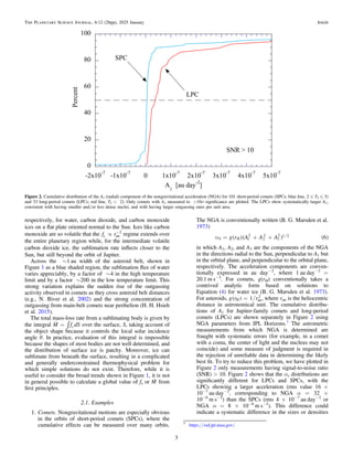
Abstract
Nongravitational forces play surprising and, sometimes, centrally important roles in shaping the motions and
properties of small planetary bodies. In the solar system, the morphologies of comets, the delivery of meteorites,
and the shapes and dynamics of asteroids and binaries are all affected by nongravitational forces. In exoplanetary
systems and debris disks, nongravitational forces affect the lifetimes of circumstellar particles and feed refractory
debris to the photospheres of the central stars. Unlike the gravitational force, which is a simple function of the well-
known separations and masses of bodies, the nongravitational forces are frequently functions of poorly known or
even unmeasurable physical properties. Here, we present order-of-magnitude descriptions of nongravitational
forces, with examples of their application.
Unified Astronomy Thesaurus concepts: Small Solar System bodies (1469); Asteroid satellites (2207); Long period
comets (933); Main-belt comets (2131); Short period comets (1452); Debris disks (363); Comets (280);
Asteroids (72)
1. Introduction
Gravity alone provides an ample description of the dynamics
and of many physical properties of planetary-mass bodies.
However, scientific interest is increasingly focused on smaller
bodies in orbit around the Sun and other stars, and small bodies
are additionally susceptible to a host of other forces. These so-
called nongravitational forces include recoil and torque from
anisotropic mass loss, radiation pressure, Poynting–Robertson
drag, Yarkovsky force, YORP torque, and forces from
magnetic interactions with the solar wind. Important examples
of phenomena that cannot be understood using gravity alone
are numerous, ranging from the motion of dust particles in
comets, the Zodiacal cloud and debris disks, to the orbital drift
of asteroids and their delivery into planet-crossing orbits, to the
centripetal shaping and disintegration of comets and asteroids,
to the formation of asteroid binaries and pairs.
Unfortunately, the research literature tends to present
nongravitational forces either in excruciating and largely
unhelpful detail or, more usually, without meaningful discus-
sion of any sort. Indeed, nongravitational forces are often
hidden as lines of code in elaborate numerical models, where
their practical role is to help to improve the fit to data by adding
extra degrees of freedom. Sadly, they sometimes do so without
giving a parallel improvement in our understanding of the
relevant physics.
The objective of the current paper is to provide a highly
simplified but nevertheless informative account of the different
nongravitational forces that are important in the solar system.
We also add some pointers to sample applications from the
literature, in a style suitable for the nonspecialist. With this in
mind, in the following, we either neglect geometrical factors
representing body shape, or approximate the relevant bodies as
spheres, with bulk density ρ [kg m−3
] and radius a [m]. The
orbits of all bodies are assumed to be circular, so that the
heliocentric distance is also the semimajor axis. Of course, real
bodies are not spherical, and real orbits are not circles. These
simplifying approximations remain useful, however, by giving
a guide to the order of magnitude of the forces and timescales
involved.
When the heliocentric distance, rH [m], is expressed in
astronomical unit, we give it the symbol rau. For example, the
flux of sunlight, Fe [W m−2
], which plays an obvious role in
several of the nongravitational forces, is given by
( )
p
= =
F
L
r
F
S
r
4
or, equivalently, , 1
H
2
au
2
where Le = 4 × 1026
W is the luminosity of the Sun, and Se =
1360 W m−2
is the solar constant.
2. Sublimation Recoil
By far the largest nongravitational force considered here is
that due to the sublimation of ice from small bodies heated by
the Sun. Sublimated volatiles freely expand into the near
vacuum of interplanetary space, carrying with them momentum
and exerting a recoil force on the ice-containing parent body.
Since sublimation is exponentially dependent on temperature,
most sublimation occurs on the hot dayside of the nucleus, and
the resulting recoil force is primarily antisolar. This sublimation
recoil force is
=
k MV
R th, where
M [kg s−1
] is the
sublimation rate, Vth [m s−1
] is the bulk speed of the
outflowing gas, and kR is a dimensionless constant that
describes the angular dependence of the flow. Purely
collimated flow would have kR = 1, while isotropic outgassing
would have kR = 0, meaning no net force on the nucleus. The
best estimate of kR is based on measurements from the
unusually well-studied comet 67P/Churyumov–Gerasimenko,
for which kR ∼ 1/2 (D. Jewitt et al. 2020). This is also the
value expected from uniform sublimation across the sunward
facing hemisphere of a spherical nucleus.
We can also write m
=
M m Qg
H , where μ is the molecular
weight of the sublimated ice, mH = 1.67 × 10⁻²⁷
kg is the mass
of the hydrogen atom, and Qg is the gas production rate in
molecules per second. Setting a
=
M S, where M = 4πρa3
/3
The Planetary Science Journal, 6:12 (26pp), 2025 January https://doi.org/10.3847/PSJ/ad9824
© 2025. The Author(s). Published by the American Astronomical Society.
Original content from this work may be used under the terms
of the Creative Commons Attribution 4.0 licence. Any further
distribution of this work must maintain attribution to the author(s) and the title
of the work, journal citation and DOI.
1](https://image.slidesharecdn.com/jewitt2025planet-250126132956-3e81e4bc/85/Nongravitational-Forces-in-Planetary-Systems-1-320.jpg)
![is the body mass, gives a nongravitational acceleration (NGA)
( )
a
m
pr
=
k m
a
Q V
3
4
2
S
R
g
H
3 th
for a spherical body of radius, a, and density ρ.
The outflow speed of the gas, Vth, is roughly equal to the
thermal speed of the constituent molecules
( )
/
pm
=
V
k T
m
8
. 3
th
B
H
1 2
⎜ ⎟
⎛
⎝
⎞
⎠
Here, kB = 1.38 × 10⁻²³
J K−1
is Boltzmann's constant, and
temperature T refers to the surface temperature of the
sublimating surface. This is typically depressed below the
local radiative equilibrium temperature because a fraction of
the absorbed solar energy that would otherwise drive radiative
cooling is instead used to break bonds between molecules in
the process of sublimation. While /
µ -
T rH
1 2
in radiative
equilibrium, the temperature of sublimating ice is an even
weaker function of heliocentric distance because of this
depression. We take Vth = 500 m s−1
at 1 au and assume for
simplicity that this speed applies across the terrestrial planet
region.
The temperature and sublimation rate per unit area, fs(T) [kg
m−2
s−1
], are connected by the energy balance equation for a
surface element of area oriented with its normal offset from the
direction of illumination by angle θ;
( ) ( ) ( ) ( )
q es
- = +
S
r
A T H T f T
1 cos . 4
s
au
2
4
Here, A and ε are the Bond albedo and emissivity of the
surface, σ = 5.67 × 10⁻⁸
W m−2
K−4
is the Stefan–Boltzmann
constant, and H(T) [J kg−1
] is the latent heat of sublimation for
the ice in question. An additional, generally small term for heat
conducted beneath the surface has been neglected from
Equation (4).
Additional information is needed to solve Equation (4). The
temperature dependence of fs can be obtained from the
Clausius–Clapeyron equation for the slope of the solid/vapor
phase boundary (the relation dP/dT = PH/(NAkT2
), where NA
is Avagadro's number, and k is the Boltzmann constant, which
is only applicable when H is independent of T) or, better, from
laboratory measurements of the sublimation vapor pressure
over ice as a function of temperature. The optical properties A
and ε have a minor effect on the solution provided A = 1 and
ε ? 0. In practice, A = 0 and ε = 0.9 are widely assumed.
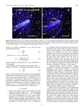
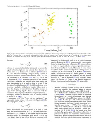
In Figure 1 we show solutions to Equation (4) for the three
most abundant cometary ices of water, carbon dioxide, and
carbon monoxide. These three, having approximate latent heats
H = 2.8 × 10⁶
J kg−1
, 0.57 × 10⁶
J kg−1
, and
0.29 × 10⁶
J kg−1
, respectively, are representative of low,
medium, and high volatility solids.
All three plotted curves trend asymptotically toward
µ -
f r
s au
2
as rau → 0. This is because the exponential
temperature dependence of fs is stronger than T4
, so that the
second term on the right of Equation (4) dominates the first at
the high temperatures found at small rau. Setting the radiative
term in Equation (4) equal to zero gives
( )
( )
~
f
S
H T r
5
s
au
2
where we have set A = 0 and θ = 0 for simplicity. Equation (5)
gives a useful approximation even at rau = 1 au, where
fs = 6 × 10⁻⁴
, 2.4 × 10⁻³
, and 4.7 × 10⁻³
kg m−2
s−1
,
Figure 1. Equilibrium sublimation mass fluxes as a function of heliocentric distance for H2O (solid black lines), CO2 (long-dashed red lines), and CO (short-dashed
blue lines) ices, computed from Equation (4). Two models are shown for each ice. The upper model for each ice shows sublimation at the subsolar temperature, taken
as the highest temperature on a spherical body, while the lower model shows sublimation at the local isothermal blackbody temperature, which is the lowest possible
temperature. The location of the asteroid belt is marked as a shaded blue rectangle, with inner and outer edges at 2.1 and 3.2 au.
2
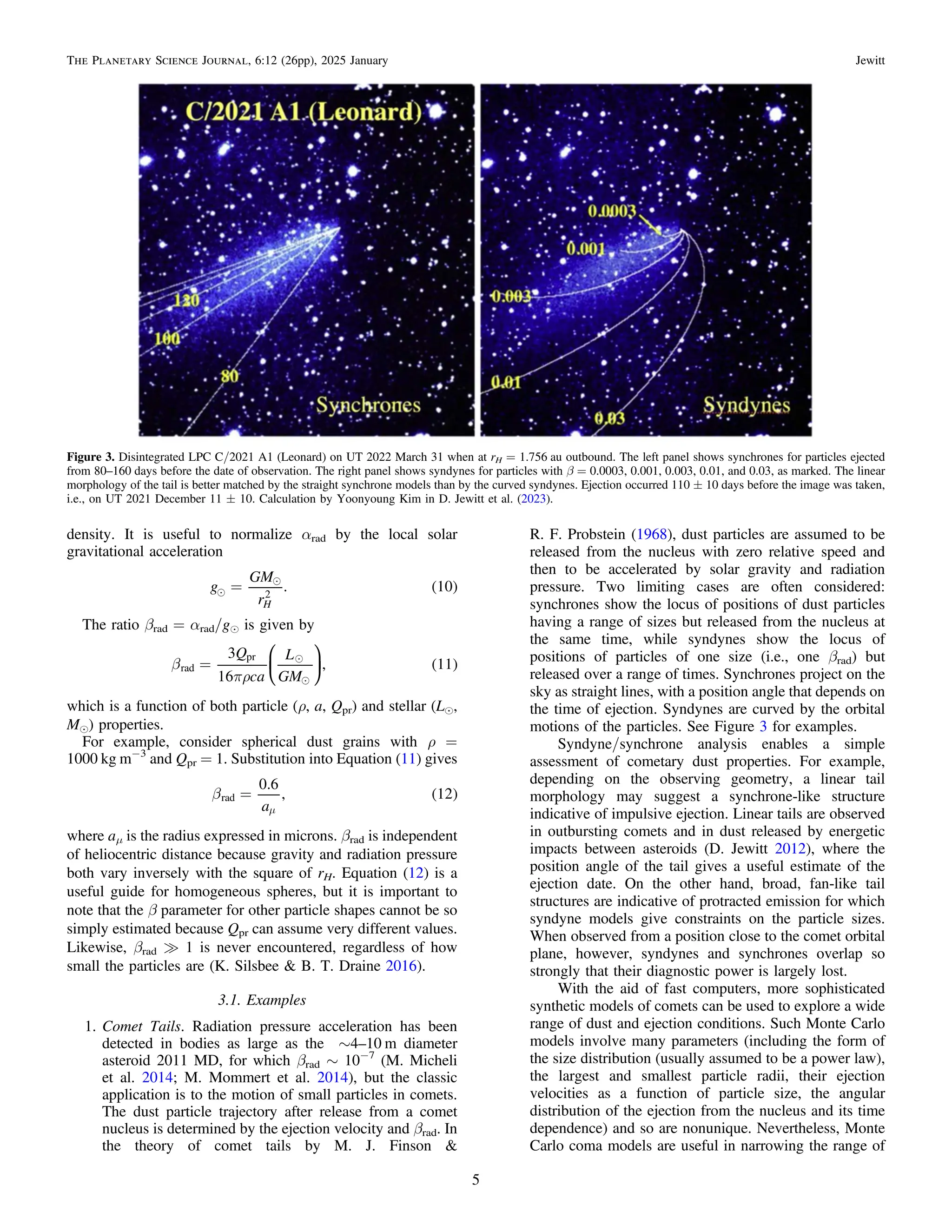
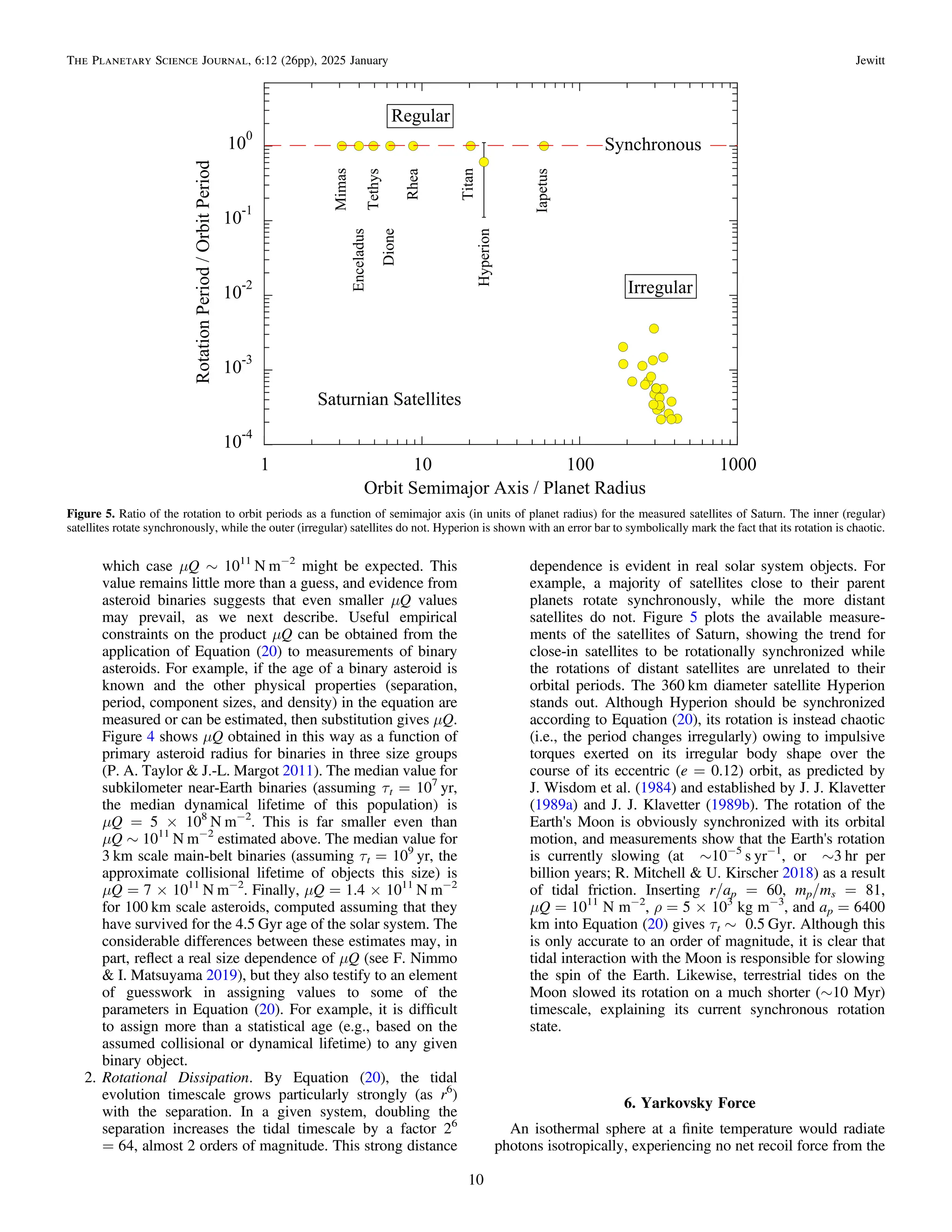
The Planetary Science Journal, 6:12 (26pp), 2025 January Jewitt](https://image.slidesharecdn.com/jewitt2025planet-250126132956-3e81e4bc/85/Nongravitational-Forces-in-Planetary-Systems-2-320.jpg)
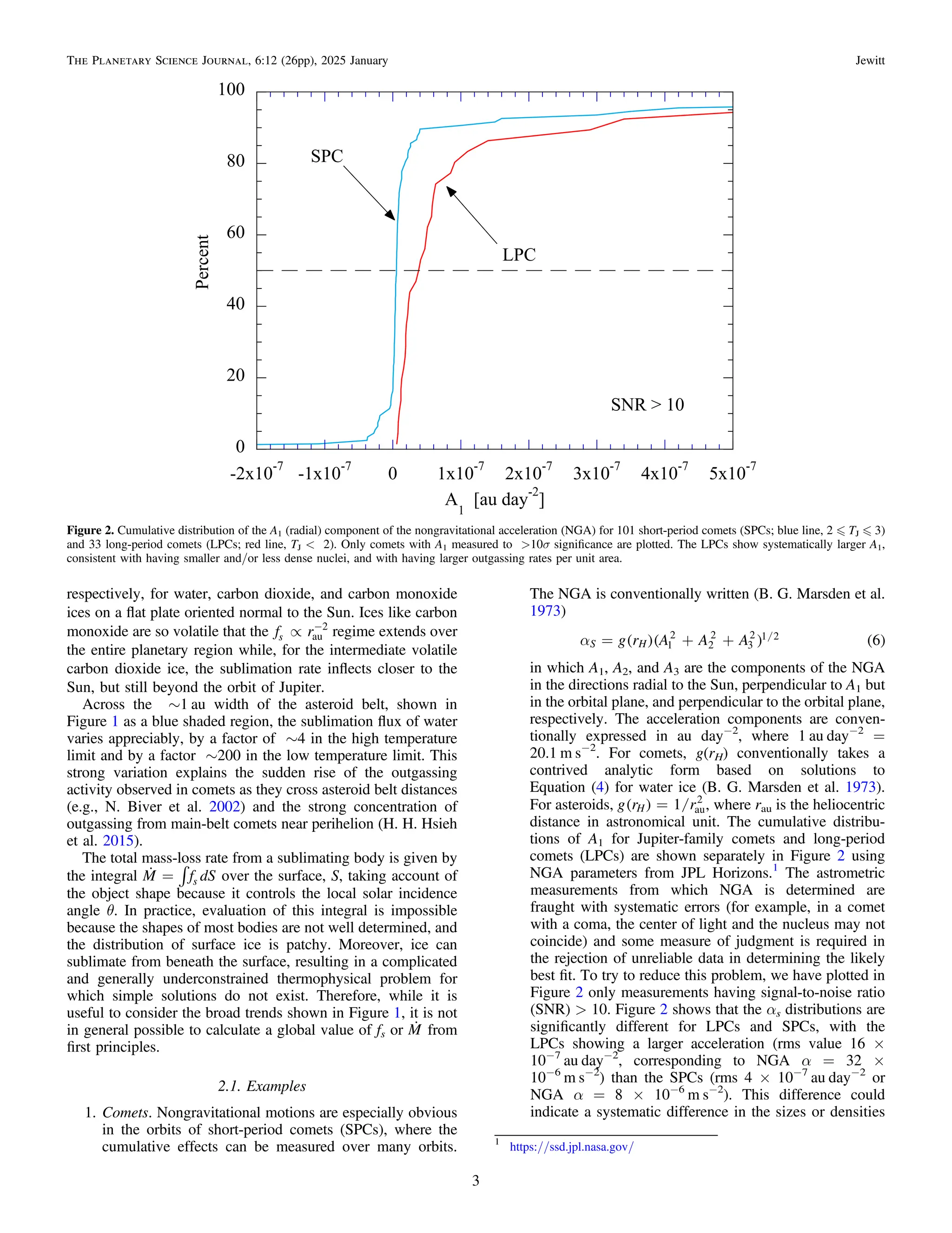
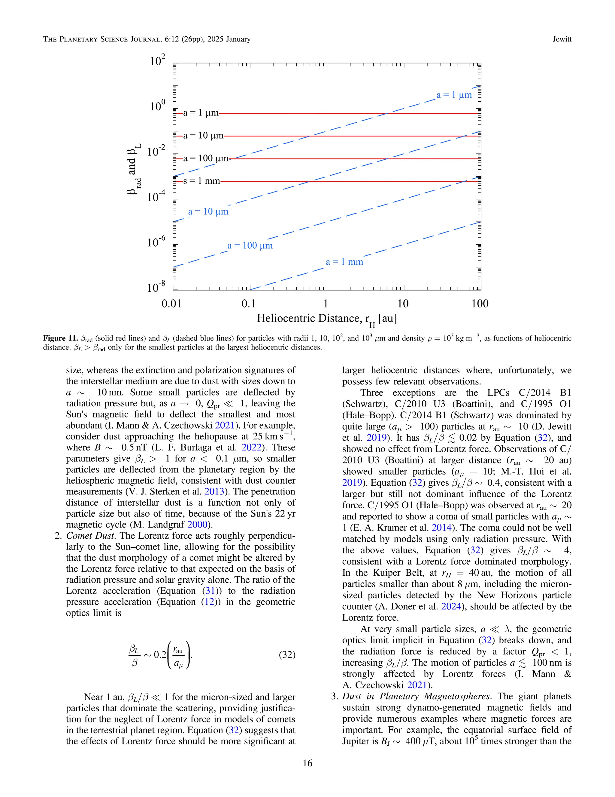
![of SPC and LPC nuclei, or a difference in the outgassing
rates per unit area of surface, or some combination of
these effects. A more prosaic explanation is a measure-
ment bias; small NGAs cannot generally be accurately
measured in LPCs because they are observed at only one
apparition, whereas SPCs can be measured over multi-
ple orbits and longer periods of time. Some 16/101
SPCs (but 0/33 LPCs) exhibit negative A1 parameters,
which indicate unexpected sunward acceleration. These
determinations, which might indicate that the astro-
metric errors are underestimated, cannot be explained by
recoil from dayside sublimation.
2. Dark Comets. Some small, apparently inert bodies exhibit
substantial NGA, yet present no evidence for outgassing.
Notable examples include the interstellar interloper 1I/
’Oumuamua (M. Micheli et al. 2018) and the ∼150 m radius
object 523599 (2003 RM; D. Farnocchia et al. 2023), as well
as a number of tiny asteroids (essentially, boulders) in the
3–15 m radius range (D. Z. Seligman et al. 2023). The
magnitude of the NGA in these evocatively named “Dark
Comets” is too large to reflect the action of radiation pressure
or Yarkovsky force but consistent with small sublimation
rates. For example, the measured acceleration of 2003
RM is α = 2 × 10⁻¹²
au day−2
(α = 4 × 10⁻¹¹
m s−2
).
From Equation (2) with kR = 0.5, μ = 18 (for H2O),
ρ = 103
kg m−3
, and Vth = 500 m s−1
, we find
Qg = 4 × 1025
s−1
(equivalent to 1 kg s−1
), which might
be small enough to have escaped detection. The Tisserand
parameter with respect to Jupiter of 2003 RM is formally that
of a comet (TJ = 2.96), in which case the presence of ice and
outgassing should not be surprising. However, D. Farnocchia
et al. (2023) preferred an origin in the outer asteroid belt and
derived a much smaller Qg ∼ 1023
s−1
. The boulders
described by D. Z. Seligman et al. (2023) can be accelerated
by sublimation at even smaller rates. For example, the
strongest (8σ) detection of NGA is in the 4 m radius boulder
2010 RF12, with A3 = (−0.17 ± 0.02) × 10−10
au day−2
(αS = 3.3 × 10⁻¹⁰
m s−2
). Substitution into Equation (2)
gives Qg ∼ 1019
s−1
(roughly 3 × 10⁻⁷
kg s−1
), which is
small enough to have escaped detection by any existing
direct technique. Radiation pressure acceleration should
be of the same order as αs but cannot account for A3,
which acts perpendicularly to the projected radial line.
The main puzzle presented by the accelerated boulders
is their implied short mass-loss lifetimes. 2020 RF12,
with mass ∼ 3 × 10⁵
kg, can sustain mass loss at
3 × 10⁻⁷
kg s−1
for only 1012
s (3 × 10⁴
yr). The
conduction timescale is even shorter (∼6 months for a
compact rock with diffusivity κ = 10−6
m2
s−1
and
∼500 yr if it is a porous dust ball with the very low
diffusivity κ = 10−9
m2
s−1
; see Appendix). As a result,
the internal temperatures of this and other boulders near
1 au would quickly equilibrate to orbit-averaged values
that are too high (∼300 K) for water ice to survive. Even
if the mass loss is intermittent, it is hard to see how such
tiny boulders could retain ice on dynamically relevant
(Myr) timescales.
3. Radiation Pressure
A radiant energy flux density Fν [J m−2
s−1
Hz−1
]
corresponds to a photon flux Fν/(hν) [photon m−2
s−1
Hz−1
], where h = 6.63 × 10⁻³⁴
J s is Planck's constant, and
hν is the energy of a photon having frequency ν. The
momentum of a single photon is h/λ = hν/c, where λ is the
wavelength, and c = 3 × 10⁸
m s−1
is the speed of light. Then,
considering the Sun as the source of photons, the flux of
momentum in photons of frequency ν → ν + dν is
dPr,ν = Fν/(hν) × (hν/c)dν. When integrated over all
frequencies, this gives a pressure
[ ] ( )
= -
P
F
c
N m 7
r
2
in which ò n
= n
¥
F F d
0
. Equation (7) is the radiation pressure.
For example, at rH = 1 au, where the flux of sunlight is given
by the solar constant, Se = 1360 W m−2
, Equation (7) gives
Pr = 4.5 × 10⁻⁶
N m−2
(about 4 million times less than the
pressure exerted by the weight of a sheet of paper). This tiny
pressure is about 105
times smaller than the pressure due to
water ice sublimation at 1 au, and is insignificant on
macroscopic bodies, but can dominate the motion of small
particles.
The force exerted by radiation impinging on a spherical grain
of radius a, is /
p
=
Q a F c
pr
2
, where Qpr is a size and
wavelength-dependent dimensionless multiplier,2
and Fe [W
m−2
] is the local flux of sunlight. The radiation pressure
acceleration is proportional to the cross section per unit mass of
the accelerated particle, and so is inversely related to the
particle size. For a spherical particle of density ρ, this results in
an acceleration
( )
a
r
=
Q F
ca
3
4
. 8
rad
pr
The inverse dependence shows that small, low-density
particles can be more strongly accelerated by radiation than
large, high-density particles. In the case of the radiation field
around the Sun, we note that the flux is given by
( )
/
p
=
F L r
4 H
2
, where Le = 4 × 1026
W is the solar
luminosity and rH is the heliocentric distance in meters.
Substituting gives
( )
a
r p
=
Q
ca
L
r
3
4 4
. 9
H
rad
pr
2
⎜ ⎟
⎛
⎝
⎞
⎠
The numerical multiplier in Equations (8) and (9) is specific
to the assumed spherical particle shape. Nevertheless, the
equations give a useful approximation to the acceleration
induced by radiation pressure as a function of particle size, and
2
Qpr is the ratio of the effective cross section for radiation pressure to the
geometric cross section of the particle. It is a function of the composition,
shape, structure, and size of a particle relative to λ, the wavelength of radiation
with which it interacts. The limits are Qpr = 1 as a/λ → 0 while Qpr →
constant as a/λ → ∞. In between, Qpr varies with a/λ in a complicated way,
reflecting interactions between electromagnetic waves as they pass, and pass
through, the particle (J. A. Burns et al. 1979; C. F. Bohren & D. R. Huff-
man 1983). In planetary science and astronomy, the zeroth order approximation
is to set Qpr = 0 for a < λ and Qpr = 1 for a λ. For many natural particle size
distributions in which the smallest particles are the most abundant, this
approximation gives rise to the rule-of-thumb that observations primarily
sample particles with a ∼ λ. Calculation of Qpr for homogeneous spheres uses
the Mie Theory. For other shapes and for porous and fractal particles of
relevance to natural solar system particles, there is no analytic theory, and Qpr
must be calculated numerically (e.g., K. Silsbee & B. T. Draine 2016).
4
The Planetary Science Journal, 6:12 (26pp), 2025 January Jewitt](https://image.slidesharecdn.com/jewitt2025planet-250126132956-3e81e4bc/85/Nongravitational-Forces-in-Planetary-Systems-4-320.jpg)
![ms, separated by a distance r, with mp ? ms. The radii of the
primary and secondary objects are ap and as, respectively. We
also assume that the densities, ρ, of the primary and secondary
are the same so that, neglecting shape specific factors,
r
~
m a
p p
3
and r
~
m a
s s
3
.
The gravitational pull of each body elongates the other along
an axis connecting their centers, with the secondary being most
deformed because of the greater mass and gravity of the
primary. If the deformation were instantaneous, this tidal bulge
would stay perfectly aligned along the line of centers.
However, the primary, in general, rotates with an angular
frequency, ωp, that is different from the orbital frequency of the
satellite, ωs, and the tidal response is not instantaneous.
Empirically, most satellites orbit beyond the corotation radius,
at which the orbital period is equal to the rotation period of the
primary body. With ωp > ωs, the tidal bulge of the primary is
carried ahead of the line of centers, and the resulting torque on
the primary acts to slow its rotation while expanding the orbit
of the secondary. In the opposite case (ωp < ωs), the tidal bulge
lags behind, and the tidal torque increases ωp while contracting
the orbit of the secondary. The latter is the case for Mars’
satellite Phobos, which orbits at 2.76 RM, far inside the
corotation radius at 6.03 RM (1 RM = 3.4 × 10⁶
m). The orbit
of Phobos will collapse into the planet because of tidal
dissipation on a (surprisingly short) timescale of a few tens of
Myr (B. A. Black & T. Mittal 2015). Mars’ other known
satellite, Deimos, orbits beyond the corotation radius at
6.92 RM and is being slowly pushed away from the planet by
tides. The finite response time and inelasticity of the material
are central to the mechanism of tidal evolution because the
misalignment of the tidal bulge creates an asymmetry upon
which gravity can exert a torque.
The gravitational force experienced from distance r is
F = Gmpms/r2
or, equivalently, /
r
~
F G a a r
p s
2 3 3 2. The gravity
of the satellite is slightly different on the near and far sides of
the primary, by an amount
( )
d
r
~ ~
F
dF
dr
a
G a a
r
. 16
p
p s
2 4 3
3
This small differential force periodically stretches and
relaxes the bodies as they rotate and orbit, doing work in the
process. The average stress due to gravitational deformation is
/
d
=
S F ap
2
[N m−2
]. The relation between the stress and the
strain (strain is the fractional change in the length scale,
s = δap/ap) is called the bulk modulus, defined as μ = S/s.
Substituting, the deformation is
( )
d
d
m
r
m
~ =
a
F
a
G a a
r
. 17
p
p
p s
2 3 3
3
The work done by a force δF applied over a distance δap is
δW ∼ δFδap. Substituting from Equations (16) and (17) gives
( )
d
r
m
=
W
G a a
r
a
. 18
p s p
2 3 3
3
2
⎛
⎝
⎜
⎞
⎠
⎟
If the material were perfectly elastic, energy added to the
body by stretching would be returned upon relaxation back to
the original shape. But in real materials, owing to internal
friction, a fraction of the energy is dissipated as heat. The
fraction lost per stretching cycle is conventionally defined as
Q−1
= δE/E (i.e., Q is the inverse of what one would expect)
and referred to as the tidal “quality factor.” High Q corresponds
to low dissipation per cycle and vice versa. Given this, and
recognizing that δW in Equation (18) is the work done per cycle
(not per second), we write the tidal power as
( )
d
d
r w
m
~
W
t
G a a
r Q
a
. 19
p s p p
2 3 3
3
2
⎜ ⎟
⎛
⎝
⎜
⎞
⎠
⎟
⎛
⎝
⎞
⎠
The key point in all of this is that the tidal power
(Equation (19)) scales with r−6
because the differential tidal
force, δF, and the deformation it causes, δap, are both
proportional to r−3
.
Finally, the timescale for dissipation to substantially change
the rotational energy is τt ∼ W/(δW/δt), where W is the
rotational energy. We take the rotational energy of the primary
to be w
~
W Ip p
2
where r
~ ~
I m a a
p p p p
2 5
is the moment of
inertia. Then,
( )
t
m w
r
~
Q
G a
m
m
r
a
20
t
p
p
p
s p
2 3 2
2 6
⎜ ⎟
⎜ ⎟
⎛
⎝
⎞
⎠
⎛
⎝
⎞
⎠
is the order-of-magnitude time needed for torques from the
satellite to substantially change the rotation of the primary.
Tides raised on the satellite by the gravity of the primary are
larger, and act to change the rotation on an even shorter
timescale, as can be seen by swapping as and ap in
Equation (20). Obviously, this derivation is highly simplified,
but it serves to show the functional dependence of the tidal
evolution timescale on material (ρ, μ, Q) and geometrical (ap,
as, r) properties.
5.2. Internal Dissipation
Even without an external force from a binary companion,
internal energy dissipation in an inelastic material can modify
the spins of individual asteroids. The loss of rotational energy
occurs when a body is rotating in a nonprincipal axis state, such
that its rotational energy is not a minimum for its shape. Then,
any element of the body is subject to a cyclically varying stress
as it rotates, which induces a variable strain, allowing internal
friction to act. The visual model is a deflected gyroscope,
which both rotates around its axis and precesses and nutates at
the same time.
We can obtain a useful expression for the functional
dependence of the damping timescale by the same dimensional
method as used for the tidal effects in Section 5.1. Precession
and nutation of the rotation axis induce time-variable stresses
that do work by cyclically compressing and relaxing the
material. The internal stress, proportional to the energy density
in the body, is S ∼ ρa2
ω2
[N m−2
], where a is the nominal size
of the body, and ω [s−1
] the relevant angular frequency. Stress
and strain (δa/a) are related through the modulus μ = S/(δa/
a), giving δa ∼ Sa/μ. Then, by analogy with Section 5.1, the
power dissipated as heat by the stress is δW/δt ∼ Sa2
δa(ω/Q),
which becomes
( )
d
d
r w
m
=
W
t
a
Q
. 21
2 7 5
This compares with the instantaneous rotational energy
W ∼ ρa5
ω2
, and the ratio of W to δW/δt gives the damping
8
The Planetary Science Journal, 6:12 (26pp), 2025 January Jewitt](https://image.slidesharecdn.com/jewitt2025planet-250126132956-3e81e4bc/85/Nongravitational-Forces-in-Planetary-Systems-8-320.jpg)

![multiplied by the moment arm, which we write as kTa, where a
is the nucleus radius and 0 „ kT „ 1 is a dimensionless
multiplier. kT = 0 corresponds to perfectly isotropic sublima-
tion with no net torque. kT = 1 corresponds to perfectly
collimated ejection tangential to the surface of the body. Then,
with a mass-loss rate μmHQg [kg s−1
] and an outflow speed Vth,
the magnitude of the torque is T = μmHQgkTVtha. The
timescale for the torque to change the spin is then
(D. Jewitt 2021)
( )
t
p r
m
~
a
m Q k V P
16
15
1
. 34
s
g T
2 4
H th
Note that, for a fixed Qg, Equation (34) has a very strong (a4
)
nucleus radius dependence. However, it is natural to expect that
the production rate, Qg, should scale with the nucleus area,
Qg ∝ a2
and, if it does, τs ∝ a2
is anticipated for the nuclei of
comets, all else being equal.
The rotational lightcurves of some comets have enabled the
measurement of spin changes (e.g., R. Kokotanekova et al.
2018), allowing τs to be directly estimated. With additional
observational constraints on ρ, a, Qg, and P, and with the use of
Equation (34), the dimensionless moment arm, kT, can be
estimated (D. Jewitt 2021). The median value is kT = 0.007,
meaning that only 0.7% of the outflow momentum is used to
torque the nucleus. Even this tiny fraction is sufficient to
quickly modify the spins of small comets.
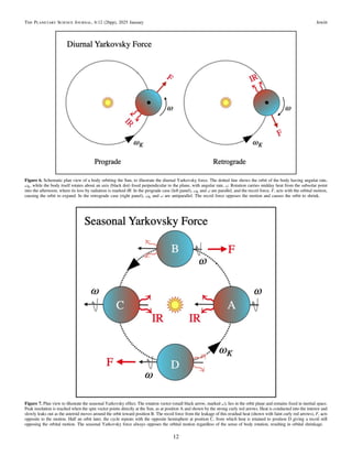
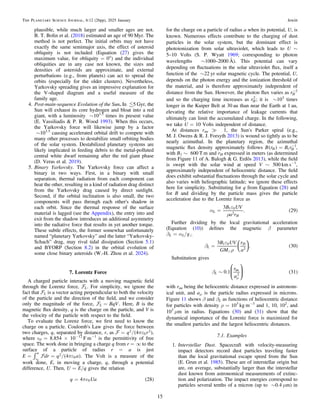
Measured values of τs as a function of a are plotted in
Figure 13. The relation
( )
t ~ a
100 35
s
2
with a in kilometers and τs in years, matches the data well
(D. Jewitt 2021). (This relation strictly applies to JFCs with
perihelia in the 1–2 au range.) Spin-up by outgassing torques
ends with rotational instability and breakup. The fragmented
nucleus of 332P/Ikeya–Murakami at rH = 1.6 au gives a good
example (Figure 14). A cloud of fragments expands from main
nucleus C, whose rotation in about 2 hr suggests rotational
instability (D. Jewitt et al. 2016).
A necessary condition for Equation (34) to remain valid is
the persistence of ice at or near the physical surface of the
nucleus for timescales τs. Near-surface ice persists because
the speed with which the ice sublimation surface erodes into the
nucleus exceeds the speed with which heat conducts into the
interior, causing fresh ice to be continually excavated. The
particular problem is that sublimation exposes refractory
particles too large to be ejected by gas drag. These should
eventually clog the surface, producing a “rubble mantle” and
inhibiting or shutting down further sublimation. How this
works in detail is not known, even after several years of in situ
investigation of the nucleus of 67P/Churyumov–Gerasimenko
by the Rosetta spacecraft (N. Attree et al. 2023). Orbital
evolution may play a role, particularly when the perihelion
distance migrates to smaller values, leading to higher
temperatures and sublimation fluxes. In the case of the active
asteroids, ice is exposed only intermittently, perhaps in
response to occasional impacts that clear a surface refractory
mantle. The duty cycle (ratio of the time spent in sublimation to
the total elapsed time) is less than 10−4
or even 10−5
, allowing
ice to persist for long times but rendering Equation (35)
inapplicable to these objects.
The significance of the short timescales indicated by
Equation (35) is that small nuclei cannot survive long once
they reach the vicinity of the Sun. This may explain the paucity
of subkilometer comet nuclei relative to power-law extrapola-
tions from larger sizes. It also complicates any attempt to relate
the populations and properties of comets near the Sun to their
Figure 13. Measured timescale for changing the rotation period, τs, as a function of the nucleus radius for SPCs with perihelia in the 1–2 au range. Filled red circles
show spin-change detections, while yellow diamonds show lower limits to the allowed spin-up timescales. Comets are identified by their numerical labels. The dashed
line shows τs = 100a2
. Data are from D. Jewitt (2021).
18
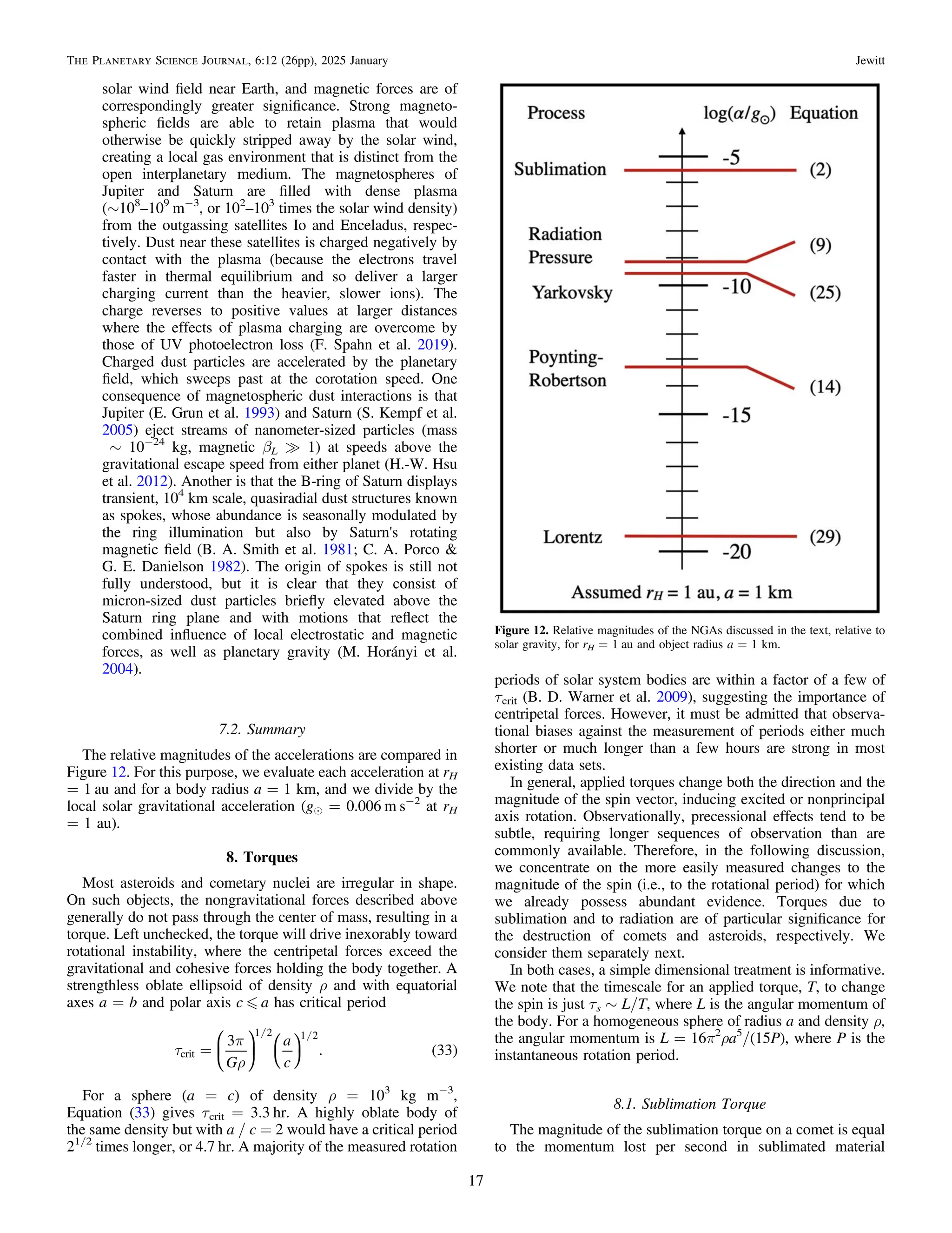
The Planetary Science Journal, 6:12 (26pp), 2025 January Jewitt](https://image.slidesharecdn.com/jewitt2025planet-250126132956-3e81e4bc/85/Nongravitational-Forces-in-Planetary-Systems-18-320.jpg)
![similarly sized counterparts in the Kuiper Belt and Oort cloud
source regions.
8.2. YORP Torque
Nonspherical bodies warmed by the Sun radiate infrared
photons, which carry away momentum and can exert a torque
(e.g., D. P. Rubincam 2000). Here we offer a simplified
treatment that captures the physical essence of the torque,
followed by some examples of its application to real bodies.
The torque is proportional to the surface area, a2
, multiplied by
the moment arm, which we write as ¢
k a
T , where
¢
k
0 1
T is
another dimensionless constant that must be empirically
determined. Again setting timescale τYORP ∼ L/T, we obtain,
( )
t
pr
= ¢
a c
k P
r
S
16
15
. 36
T
YORP
2
au
2
⎜ ⎟
⎛
⎝
⎞
⎠
The dimensionless moment arm, ¢
kT , is such a sensitive
function of the body shape, surface roughness, and thermo-
physical parameters, all of which are unknown for most
asteroids, that it cannot in general be calculated. Instead, we
rely on measurements of the few asteroids where changes in the
rotation periods can be measured and the other parameters in
Equation (36) are constrained. These asteroids are listed in
Table 1, where measurements of a, P, and dP/dt are from the
Figure 14. Labeled fragments released from component C of comet 332P/Ikeya–Murakami in 2015 and separating from it at speeds 0.06–4 m s−1
. C itself rotates
with a probable period near 2 hr, suggesting rotational instability as the cause of the release of fragments. Data are from D. Jewitt et al. (2016).
Table 1
YORP Timescalesa
Object D b
P c
dω/dtd
τe
(1620) Geographos 2.56 5.22 1.14 ± 0.03 6.9 ± 0.2
(1685) Toro 3.5 10.20 0.33 ± 0.03 12.3 ± 1.0
(1862) Apollo 1.55 3.07 4.94 ± 0.09 2.7 ± 0.05
(2100) Ra-Shalom 2.30 19.82 <0.6 >3.5
(3103) Eger 1.78 5.71 <1.5 >4.8
(10115) 1992 SK 1.0 7.32 8.3 ± 0.6 0.68 ± 0.05
(25143) Itokawa 0.32 12.13 3.54 ± 0.38 1.0 ± 0.1
(54509) YORP 0.11 0.20 350 ± 35 0.59 ± 0.05
(85989) 1999 JD6 1.53 7.66 <1.2 >4.5
(85990) 1999 JV6 0.44 6.54 <7.2 >0.9
(68346) 2001 KZ66 0.80 4.99 8.43 ± 0.69 1.0 ± 0.1
(101955) Bennu 0.49 4.30 6.34 ± 0.91 1.5 ± 0.2
(138852) 2000 WN10 0.3 4.46 5.5 ± 0.7 1.7 ± 0.2
(161989) Cacus 1.0 3.76 1.86 ± 0.09 5.9 ± 0.3
Notes.
a
Asteroid data from J. Ďurech et al. (2024).
b
Diameter in kilometers.
c
Rotation period in hours.
d
Rate of change of the angular frequency ×10−8
[radian day−1
]. Values from
J. Ďurech et al. (2024) that are statistically insignificant are listed as 3σ upper
limits.
e
YORP time, Myr.
19
The Planetary Science Journal, 6:12 (26pp), 2025 January Jewitt](https://image.slidesharecdn.com/jewitt2025planet-250126132956-3e81e4bc/85/Nongravitational-Forces-in-Planetary-Systems-19-320.jpg)
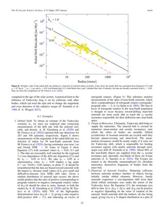
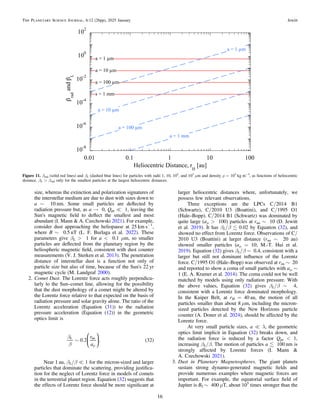
![compilation by J. Ďurech et al. (2024; see also B. Rozitis &
S. F. Green 2013 and references therein). Figure 15 shows the
YORP timescale computed from τYORP = P/(dP/dt), with
dP/dt = − (P2
/2π)dω/dt and dω/dt from the Table. τYORP is
shown as a function of the asteroid radius with each object
labeled by its identifying number. The asteroids used in
Figure 15 all have semimajor axis ∼1 au.
The Figure clearly shows that τYORP and a are correlated,
with larger asteroids showing longer YORP timescales.
Adopting the form of Equation (36) and the data from
Figure 15, we estimate
[ ] ( )
t ~ a r
4.5 Myr 37
YORP
2
au
2
where a is the radius in kilometers, and rau is the semimajor axis in
astronomical unit. By this equation, across the asteroid main belt
from 2.1–3.3 au, a 1 km radius asteroid would have τYORP ∼
20–50 Myr. Setting τYORP = 4500 Myr in Equation (37) and
solving for a, we find that YORP can influence the spins of main-
belt asteroids up to a ∼ 10–14 km. This is in broad agreement with
the asteroid rotational barrier (Figure 16), which is prominent for
asteroids up to about 10 km in diameter (implying spin-up and
breakup for smaller bodies) but less evident beyond about 30 km,
where primordial spin is likely preserved (e.g., P. Pravec et al.
2002). It should be noted that the dashed blue line in Figure 15
shows a least-squares fit to the data, weighted by the estimated
uncertainties on τYORP (but not on a). It gives τYORP ∝ a1.87±0.04
.
Although the value of the index is formally (3σ) smaller than the
expected value, τYORP ∝ a2
from Equation (36) (shown in the
Figure as a solid red line), the difference is likely not important
given the existence of systematic errors in the sample.
A major limitation to the order-of-magnitude estimates of the
torque timescales, both for sublimation (Equation (35)) and for
YORP (Equation (37)), concerns the stability of the torque. In
comets, the magnitude and direction of the outgassing torque
depend on the surface distribution and angular dependence of the
outgassing. As the surface erodes, we expect the spatial and
angular distribution of outgassing sources to change, altering the
torque. For most comets, we possess few or no observational
constraints on the areal distribution of sources or their evolution.
Indeed, in situ measurements from 67P/Churyumov–Gerasi-
menko show the difficulty in modeling this process even given
the most detailed data (N. Attree et al. 2023). Likewise, the
YORP torque is highly sensitive to the surface shape and texture
and can change in magnitude and even direction in response to
minor surface changes (T. S. Statler 2009). Empirical but
indirect evidence for this comes from asteroid (162173) Ryugu
(a ∼ 0.5 km), which has the characteristic diamond shape
indicative of rotational instability but a current rotation period
near 7.6 hr. The rotation of Ryugu may have slowed in response
to a changing YORP torque, leaving its equatorial ridge as
evidence of its previously rapid spin. Spin evolution in the
presence of a changing torque may be more akin to a random
walk process than to the steady change implicit in Equations (35)
and (37) (W. F. Bottke et al. 2015; T. S. Statler 2015). The
relevant spin-change timescales would then be much longer than
estimated here. Unfortunately, we possess too little information
to address this problem with any confidence.
8.3. Examples
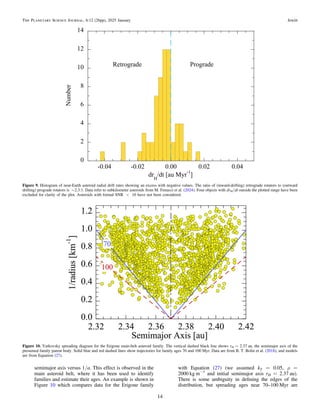
1. Asteroid Spin Barrier. The distribution of asteroid spin
frequencies as a function of absolute magnitude, H, is
shown in Figure 16. H is related to the asteroid diameter
Figure 15. Empirical timescale for YORP spin-change for asteroids near 1 au as a function of the asteroid radius [km]. Data with upward pointing arrows represent 3σ
lower limits to τYORP based on nondetections of rotational acceleration. They are not included in the fit. The dashed blue line shows a weighted least-squares fit to the
detections, τYORP ∝ a1.87±0.04
. The solid red line shows Equation (37) for rau = 1. Data from J. Ďurech et al. (2024).
20
The Planetary Science Journal, 6:12 (26pp), 2025 January Jewitt](https://image.slidesharecdn.com/jewitt2025planet-250126132956-3e81e4bc/85/Nongravitational-Forces-in-Planetary-Systems-20-320.jpg)
![by D = 1329 × 10−0.2H
/p1/2
, where p is the geometric
albedo. (We assumed p = 0.1 to calculate the diameters
shown along the top axis of the Figure; in fact, the
albedos of a majority of the plotted asteroids have not
been measured.) Few asteroids larger than D ∼ 0.2 km
have periods shorter than ∼2.4 hr (marked in the Figure
by a horizontal, dashed red line) whereas, among smaller
asteroids, more rapid rotation is common (P. Pravec et al.
2002; J. Beniyama et al. 2022). This is (admittedly
indirect) evidence for spin-up by YORP of a “bunch of
grapes” internal structure in which centripetal accelera-
tions in asteroids with periods 2.4 hr result in mass
shedding or breakup into smaller, more cohesive
component units. Measured periods of some tiny
asteroids are as short as a few seconds (J. Beniyama
et al. 2022).
2. Asteroid Reshaping and Pair Formation. Separate
evidence for rotational reshaping of asteroids is provided
by the morphologies of some spacecraft-visited asteroids,
which show approximate rotational symmetry but with an
equatorial skirt consisting of material that has evidently
migrated from higher latitudes (D. J. Scheeres 2015).
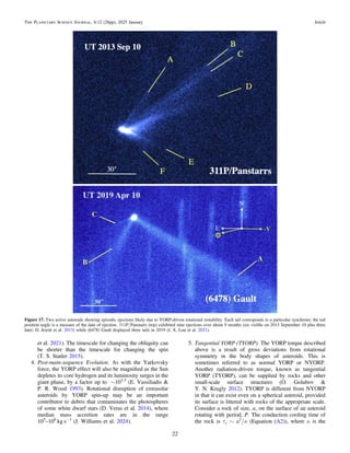
New observations of asteroids have also revealed cases of
episodic (311P/Panstarrs (2013 P5); D. Jewitt et al.
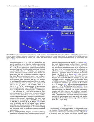
2013) and catastrophic (P/2013 R3, Catalina-Pan-
STARRS; D. Jewitt et al. 2017) mass loss that indicate
mass shedding and rotational breakup in real-time. Like
311P, the 2 km radius asteroid (6478) Gault displayed
episodic mass loss consistent with mass shedding
instability and also has a rotation period (2.55 hr)
suggestively close to the rotational barrier (J. X. Luu
et al. 2021). See Figures 17 and 18. Extreme end-cases of
continued spin-up under the influence of YORP torque
include rubble-pile disaggregation (D. J. Scheeres 2018),
which might have been observed in P/2013 R3
(Figure 18), and the formation of asteroid binaries and
pairs. These are independent asteroids with orbital
element similarities that are statistically improbable by
chance alone (S. A. Jacobson & D. J. Scheeres 2011;
K. J. Walsh 2018). Asteroid pairs show a systematic
relation between the angular frequency of the primary
and the secondary/primary mass ratio, such that high
mass ratio pairs have distinctly long-period primaries
(P. Pravec et al. 2019). This is a result of the combined
action of primary spin-up by YORP torques and
tidal transfer of rotational energy from the primary,
needed to expand the orbit of the secondary. Sudden
mass transfer events on asteroids should lead to excited
rotation; relevant observations are difficult and presently
lacking.
3. Spin Alignment. It might be expected that collisionally
produced asteroid families should have a very broad or
even random distribution of spin vectors. S. M. Slivan
(2002) discovered that the spin vectors of the Koronis
family asteroids are instead clustered, with obliquities
preferentially near 45° and 170°. This clustering was
subsequently modeled as a consequence of interaction
between gravitational and YORP torques (D. Vokrouhli-
cký et al. 2003). Subsequent work showed that the
general asteroid obliquity distribution is size dependent
(J. Hanuš et al. 2011). Objects of diameter 30 km are
more likely to have YORP-aligned obliquities near 0° and
180° (see Figure 7(a) of J. Hanuš et al. 2011). The
efficacy of alignment by radiation torques is dependent
not just on size but also on many poorly constrained
physical and thermophysical parameters (O. Golubov
Figure 16. Distribution of asteroid rotational frequencies [rotations day−1
] as a function of absolute magnitude, H. Approximate asteroid diameters are marked at the
top of the Figure, while their rotation periods are indicated on the right-hand axis. The dashed red line marking the “spin barrier” at P−1
∼ 10 day−1
shows that few
asteroids with diameter D 0.2 km have periods <2.4 hr. Data are from B. D. Warner et al. (2009; updated 2023 October 1 from the F-D Basic file at http://www.
MinorPlanet.info/php/lcdb.php).
21
The Planetary Science Journal, 6:12 (26pp), 2025 January Jewitt](https://image.slidesharecdn.com/jewitt2025planet-250126132956-3e81e4bc/85/Nongravitational-Forces-in-Planetary-Systems-21-320.jpg)
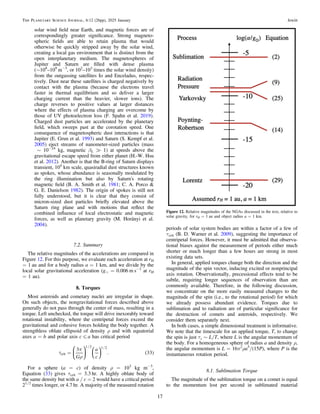
![radii of 1 km and 0.1 km, respectively. The sublimation model
was computed assuming ( )
q
cos = 1/2 in Equation (4), which
lies in between the high- and low-temperature limit models in
Figure 1, and is scaled to timescale τs = 102
yr on a 1 km
nucleus at 1 au, in agreement with the data (Figure 13).
Figure 19 shows that, for a given object size and distances 5
or 6 au, the timescales for spin-change are ∼105
times shorter
for sublimation torques than for YORP torques. Beyond
Saturn, the diminishing water ice sublimation rate pushes the
sublimation timescale to exceed that from YORP, and, in
practice, both processes become so slow in the middle and
outer solar system as to become largely irrelevant.
Acknowledgments
I thank Marco Fenucci for providing a digital table of his
Yarkovsky drift measurements, Pedro Lacerda, Jane Luu, Joe
Masiero, Darryl Seligman, David Vokrouhlicky, Emerson
Whittaker, and an anonymous referee for comments.
Appendix
Thermophysics
To gain some physical insight into how the thermophysical
parameters of an asteroid might affect Yarkovsky and YORP,
we consider the one-dimensional heat conduction equation
( )
r
=
c
T
t
k
T
z
, A1
p
2
2
where T is the temperature, k is the thermal conductivity, ρ is
the bulk density, and cp is the specific heat capacity of the
asteroid surface materials. Dimensionalizing this equation
gives the timescale for heat to conduct over a distance ℓ as
( )
t
k
k
r
~ =
ℓ k
c
where A2
C
p
2
and κ [m2
s−1
] is the thermal diffusivity.4
For a body with
rotation period P, we set τC = P and use Equation (A2) to find
the distance over which heat can conduct in one rotation period
as ℓ = (κP)1/2
, which defines the diurnal thermal skin depth on
the asteroid. An exact solution of Equation (A1) would show
that T varies with depth as a damped sinusoid, with (κP)1/2
being the e-folding length scale of the damping, but our order-
of-magnitude approximation is sufficient here. On a spherical
body with radius a, the heat contained within the skin depth, ℓ,
is
( ) ( )
/
p r k
=
H a P c T
4 A3
p
2 1 2
where cp [J K−1
kg−1
] is the specific heat capacity of the shell.
Loss of heat by radiation into space occurs at the rate
( )
p s
=
dH
dt
a T
4 A4
2 4
where σ = 5.67 × 10⁻⁸
W m−2
K−4
is the Stefan–Boltzmann
radiation constant, and we assume emissivity ε = 1. The order-
Figure 19. The YORP (blue) and water ice sublimation (red) timescales plotted as a function of rH. Timescales for objects 1 km radius (solid lines) and 0.1 km in
radius (dashed lines) are shown. The shaded band marks the approximate location of the main asteroid belt, across which sublimation supplies a ∼105
times stronger
torque if near-surface ice is present.
4
Diffusivity appears directly in Equation (A1) and is the natural measure of
thermal response of a material through Equation (A2). In planetary science, the
use of thermal inertia is instead widely preferred. Thermal inertia is defined by
( ) /
r
=
I k cp
1 2, which has the somewhat uncomfortable units [J m−2
s−1/2
K−1
].
Solid dielectrics (e.g., nonporous rocks) have I ∼ 103
J m−2
s−1/2
K−1
, while
the finest dust, as found in the regoliths of small outer solar system bodies, has
I ∼ 1 to 10 J m−2
s−1/2
K−1
(C. Ferrari 2018). Asteroid inertias in the range 10
„ I „ 100 J m−2
s−1/2
K−1
are common (E. M. MacLennan &
J. P. Emery 2021).
24
The Planetary Science Journal, 6:12 (26pp), 2025 January Jewitt](https://image.slidesharecdn.com/jewitt2025planet-250126132956-3e81e4bc/85/Nongravitational-Forces-in-Planetary-Systems-24-320.jpg)

![Nongravitational Forces in Planetary Systems
David Jewitt
Department of Earth, Planetary and Space Sciences, University of California at Los Angeles, Los Angeles, CA 90095-1567, USA; djewitt@gmail.com
Received 2024 September 12; revised 2024 November 24; accepted 2024 November 25; published 2025 January 16
Abstract
Nongravitational forces play surprising and, sometimes, centrally important roles in shaping the motions and
properties of small planetary bodies. In the solar system, the morphologies of comets, the delivery of meteorites,
and the shapes and dynamics of asteroids and binaries are all affected by nongravitational forces. In exoplanetary
systems and debris disks, nongravitational forces affect the lifetimes of circumstellar particles and feed refractory
debris to the photospheres of the central stars. Unlike the gravitational force, which is a simple function of the well-
known separations and masses of bodies, the nongravitational forces are frequently functions of poorly known or
even unmeasurable physical properties. Here, we present order-of-magnitude descriptions of nongravitational
forces, with examples of their application.
Unified Astronomy Thesaurus concepts: Small Solar System bodies (1469); Asteroid satellites (2207); Long period
comets (933); Main-belt comets (2131); Short period comets (1452); Debris disks (363); Comets (280);
Asteroids (72)
1. Introduction
Gravity alone provides an ample description of the dynamics
and of many physical properties of planetary-mass bodies.
However, scientific interest is increasingly focused on smaller
bodies in orbit around the Sun and other stars, and small bodies
are additionally susceptible to a host of other forces. These so-
called nongravitational forces include recoil and torque from
anisotropic mass loss, radiation pressure, Poynting–Robertson
drag, Yarkovsky force, YORP torque, and forces from
magnetic interactions with the solar wind. Important examples
of phenomena that cannot be understood using gravity alone
are numerous, ranging from the motion of dust particles in
comets, the Zodiacal cloud and debris disks, to the orbital drift
of asteroids and their delivery into planet-crossing orbits, to the
centripetal shaping and disintegration of comets and asteroids,
to the formation of asteroid binaries and pairs.
Unfortunately, the research literature tends to present
nongravitational forces either in excruciating and largely
unhelpful detail or, more usually, without meaningful discus-
sion of any sort. Indeed, nongravitational forces are often
hidden as lines of code in elaborate numerical models, where
their practical role is to help to improve the fit to data by adding
extra degrees of freedom. Sadly, they sometimes do so without
giving a parallel improvement in our understanding of the
relevant physics.
The objective of the current paper is to provide a highly
simplified but nevertheless informative account of the different
nongravitational forces that are important in the solar system.
We also add some pointers to sample applications from the
literature, in a style suitable for the nonspecialist. With this in
mind, in the following, we either neglect geometrical factors
representing body shape, or approximate the relevant bodies as
spheres, with bulk density ρ [kg m−3
] and radius a [m]. The
orbits of all bodies are assumed to be circular, so that the
heliocentric distance is also the semimajor axis. Of course, real
bodies are not spherical, and real orbits are not circles. These
simplifying approximations remain useful, however, by giving
a guide to the order of magnitude of the forces and timescales
involved.
When the heliocentric distance, rH [m], is expressed in
astronomical unit, we give it the symbol rau. For example, the
flux of sunlight, Fe [W m−2
], which plays an obvious role in
several of the nongravitational forces, is given by
( )
p
= =
F
L
r
F
S
r
4
or, equivalently, , 1
H
2
au
2
where Le = 4 × 1026
W is the luminosity of the Sun, and Se =
1360 W m−2
is the solar constant.
2. Sublimation Recoil
By far the largest nongravitational force considered here is
that due to the sublimation of ice from small bodies heated by
the Sun. Sublimated volatiles freely expand into the near
vacuum of interplanetary space, carrying with them momentum
and exerting a recoil force on the ice-containing parent body.
Since sublimation is exponentially dependent on temperature,
most sublimation occurs on the hot dayside of the nucleus, and
the resulting recoil force is primarily antisolar. This sublimation
recoil force is
=
k MV
R th, where
M [kg s−1
] is the
sublimation rate, Vth [m s−1
] is the bulk speed of the
outflowing gas, and kR is a dimensionless constant that
describes the angular dependence of the flow. Purely
collimated flow would have kR = 1, while isotropic outgassing
would have kR = 0, meaning no net force on the nucleus. The
best estimate of kR is based on measurements from the
unusually well-studied comet 67P/Churyumov–Gerasimenko,
for which kR ∼ 1/2 (D. Jewitt et al. 2020). This is also the
value expected from uniform sublimation across the sunward
facing hemisphere of a spherical nucleus.
We can also write m
=
M m Qg
H , where μ is the molecular
weight of the sublimated ice, mH = 1.67 × 10⁻²⁷
kg is the mass
of the hydrogen atom, and Qg is the gas production rate in
molecules per second. Setting a
=
M S, where M = 4πρa3
/3
The Planetary Science Journal, 6:12 (26pp), 2025 January https://doi.org/10.3847/PSJ/ad9824
© 2025. The Author(s). Published by the American Astronomical Society.
Original content from this work may be used under the terms
of the Creative Commons Attribution 4.0 licence. Any further
distribution of this work must maintain attribution to the author(s) and the title
of the work, journal citation and DOI.
1](https://image.slidesharecdn.com/jewitt2025planet-250126132956-3e81e4bc/75/Nongravitational-Forces-in-Planetary-Systems-1-2048.jpg)
![is the body mass, gives a nongravitational acceleration (NGA)
( )
a
m
pr
=
k m
a
Q V
3
4
2
S
R
g
H
3 th
for a spherical body of radius, a, and density ρ.
The outflow speed of the gas, Vth, is roughly equal to the
thermal speed of the constituent molecules
( )
/
pm
=
V
k T
m
8
. 3
th
B
H
1 2
⎜ ⎟
⎛
⎝
⎞
⎠
Here, kB = 1.38 × 10⁻²³
J K−1
is Boltzmann's constant, and
temperature T refers to the surface temperature of the
sublimating surface. This is typically depressed below the
local radiative equilibrium temperature because a fraction of
the absorbed solar energy that would otherwise drive radiative
cooling is instead used to break bonds between molecules in
the process of sublimation. While /
µ -
T rH
1 2
in radiative
equilibrium, the temperature of sublimating ice is an even
weaker function of heliocentric distance because of this
depression. We take Vth = 500 m s−1
at 1 au and assume for
simplicity that this speed applies across the terrestrial planet
region.
The temperature and sublimation rate per unit area, fs(T) [kg
m−2
s−1
], are connected by the energy balance equation for a
surface element of area oriented with its normal offset from the
direction of illumination by angle θ;
( ) ( ) ( ) ( )
q es
- = +
S
r
A T H T f T
1 cos . 4
s
au
2
4
Here, A and ε are the Bond albedo and emissivity of the
surface, σ = 5.67 × 10⁻⁸
W m−2
K−4
is the Stefan–Boltzmann
constant, and H(T) [J kg−1
] is the latent heat of sublimation for
the ice in question. An additional, generally small term for heat
conducted beneath the surface has been neglected from
Equation (4).
Additional information is needed to solve Equation (4). The
temperature dependence of fs can be obtained from the
Clausius–Clapeyron equation for the slope of the solid/vapor
phase boundary (the relation dP/dT = PH/(NAkT2
), where NA
is Avagadro's number, and k is the Boltzmann constant, which
is only applicable when H is independent of T) or, better, from
laboratory measurements of the sublimation vapor pressure
over ice as a function of temperature. The optical properties A
and ε have a minor effect on the solution provided A = 1 and
ε ? 0. In practice, A = 0 and ε = 0.9 are widely assumed.
In Figure 1 we show solutions to Equation (4) for the three
most abundant cometary ices of water, carbon dioxide, and
carbon monoxide. These three, having approximate latent heats
H = 2.8 × 10⁶
J kg−1
, 0.57 × 10⁶
J kg−1
, and
0.29 × 10⁶
J kg−1
, respectively, are representative of low,
medium, and high volatility solids.
All three plotted curves trend asymptotically toward
µ -
f r
s au
2
as rau → 0. This is because the exponential
temperature dependence of fs is stronger than T4
, so that the
second term on the right of Equation (4) dominates the first at
the high temperatures found at small rau. Setting the radiative
term in Equation (4) equal to zero gives
( )
( )
~
f
S
H T r
5
s
au
2
where we have set A = 0 and θ = 0 for simplicity. Equation (5)
gives a useful approximation even at rau = 1 au, where
fs = 6 × 10⁻⁴
, 2.4 × 10⁻³
, and 4.7 × 10⁻³
kg m−2
s−1
,
Figure 1. Equilibrium sublimation mass fluxes as a function of heliocentric distance for H2O (solid black lines), CO2 (long-dashed red lines), and CO (short-dashed
blue lines) ices, computed from Equation (4). Two models are shown for each ice. The upper model for each ice shows sublimation at the subsolar temperature, taken
as the highest temperature on a spherical body, while the lower model shows sublimation at the local isothermal blackbody temperature, which is the lowest possible
temperature. The location of the asteroid belt is marked as a shaded blue rectangle, with inner and outer edges at 2.1 and 3.2 au.
2
The Planetary Science Journal, 6:12 (26pp), 2025 January Jewitt](https://image.slidesharecdn.com/jewitt2025planet-250126132956-3e81e4bc/75/Nongravitational-Forces-in-Planetary-Systems-2-2048.jpg)
![of SPC and LPC nuclei, or a difference in the outgassing
rates per unit area of surface, or some combination of
these effects. A more prosaic explanation is a measure-
ment bias; small NGAs cannot generally be accurately
measured in LPCs because they are observed at only one
apparition, whereas SPCs can be measured over multi-
ple orbits and longer periods of time. Some 16/101
SPCs (but 0/33 LPCs) exhibit negative A1 parameters,
which indicate unexpected sunward acceleration. These
determinations, which might indicate that the astro-
metric errors are underestimated, cannot be explained by
recoil from dayside sublimation.
2. Dark Comets. Some small, apparently inert bodies exhibit
substantial NGA, yet present no evidence for outgassing.
Notable examples include the interstellar interloper 1I/
’Oumuamua (M. Micheli et al. 2018) and the ∼150 m radius
object 523599 (2003 RM; D. Farnocchia et al. 2023), as well
as a number of tiny asteroids (essentially, boulders) in the
3–15 m radius range (D. Z. Seligman et al. 2023). The
magnitude of the NGA in these evocatively named “Dark
Comets” is too large to reflect the action of radiation pressure
or Yarkovsky force but consistent with small sublimation
rates. For example, the measured acceleration of 2003
RM is α = 2 × 10⁻¹²
au day−2
(α = 4 × 10⁻¹¹
m s−2
).
From Equation (2) with kR = 0.5, μ = 18 (for H2O),
ρ = 103
kg m−3
, and Vth = 500 m s−1
, we find
Qg = 4 × 1025
s−1
(equivalent to 1 kg s−1
), which might
be small enough to have escaped detection. The Tisserand
parameter with respect to Jupiter of 2003 RM is formally that
of a comet (TJ = 2.96), in which case the presence of ice and
outgassing should not be surprising. However, D. Farnocchia
et al. (2023) preferred an origin in the outer asteroid belt and
derived a much smaller Qg ∼ 1023
s−1
. The boulders
described by D. Z. Seligman et al. (2023) can be accelerated
by sublimation at even smaller rates. For example, the
strongest (8σ) detection of NGA is in the 4 m radius boulder
2010 RF12, with A3 = (−0.17 ± 0.02) × 10−10
au day−2
(αS = 3.3 × 10⁻¹⁰
m s−2
). Substitution into Equation (2)
gives Qg ∼ 1019
s−1
(roughly 3 × 10⁻⁷
kg s−1
), which is
small enough to have escaped detection by any existing
direct technique. Radiation pressure acceleration should
be of the same order as αs but cannot account for A3,
which acts perpendicularly to the projected radial line.
The main puzzle presented by the accelerated boulders
is their implied short mass-loss lifetimes. 2020 RF12,
with mass ∼ 3 × 10⁵
kg, can sustain mass loss at
3 × 10⁻⁷
kg s−1
for only 1012
s (3 × 10⁴
yr). The
conduction timescale is even shorter (∼6 months for a
compact rock with diffusivity κ = 10−6
m2
s−1
and
∼500 yr if it is a porous dust ball with the very low
diffusivity κ = 10−9
m2
s−1
; see Appendix). As a result,
the internal temperatures of this and other boulders near
1 au would quickly equilibrate to orbit-averaged values
that are too high (∼300 K) for water ice to survive. Even
if the mass loss is intermittent, it is hard to see how such
tiny boulders could retain ice on dynamically relevant
(Myr) timescales.
3. Radiation Pressure
A radiant energy flux density Fν [J m−2
s−1
Hz−1
]
corresponds to a photon flux Fν/(hν) [photon m−2
s−1
Hz−1
], where h = 6.63 × 10⁻³⁴
J s is Planck's constant, and
hν is the energy of a photon having frequency ν. The
momentum of a single photon is h/λ = hν/c, where λ is the
wavelength, and c = 3 × 10⁸
m s−1
is the speed of light. Then,
considering the Sun as the source of photons, the flux of
momentum in photons of frequency ν → ν + dν is
dPr,ν = Fν/(hν) × (hν/c)dν. When integrated over all
frequencies, this gives a pressure
[ ] ( )
= -
P
F
c
N m 7
r
2
in which ò n
= n
¥
F F d
0
. Equation (7) is the radiation pressure.
For example, at rH = 1 au, where the flux of sunlight is given
by the solar constant, Se = 1360 W m−2
, Equation (7) gives
Pr = 4.5 × 10⁻⁶
N m−2
(about 4 million times less than the
pressure exerted by the weight of a sheet of paper). This tiny
pressure is about 105
times smaller than the pressure due to
water ice sublimation at 1 au, and is insignificant on
macroscopic bodies, but can dominate the motion of small
particles.
The force exerted by radiation impinging on a spherical grain
of radius a, is /
p
=
Q a F c
pr
2
, where Qpr is a size and
wavelength-dependent dimensionless multiplier,2
and Fe [W
m−2
] is the local flux of sunlight. The radiation pressure
acceleration is proportional to the cross section per unit mass of
the accelerated particle, and so is inversely related to the
particle size. For a spherical particle of density ρ, this results in
an acceleration
( )
a
r
=
Q F
ca
3
4
. 8
rad
pr
The inverse dependence shows that small, low-density
particles can be more strongly accelerated by radiation than
large, high-density particles. In the case of the radiation field
around the Sun, we note that the flux is given by
( )
/
p
=
F L r
4 H
2
, where Le = 4 × 1026
W is the solar
luminosity and rH is the heliocentric distance in meters.
Substituting gives
( )
a
r p
=
Q
ca
L
r
3
4 4
. 9
H
rad
pr
2
⎜ ⎟
⎛
⎝
⎞
⎠
The numerical multiplier in Equations (8) and (9) is specific
to the assumed spherical particle shape. Nevertheless, the
equations give a useful approximation to the acceleration
induced by radiation pressure as a function of particle size, and
2
Qpr is the ratio of the effective cross section for radiation pressure to the
geometric cross section of the particle. It is a function of the composition,
shape, structure, and size of a particle relative to λ, the wavelength of radiation
with which it interacts. The limits are Qpr = 1 as a/λ → 0 while Qpr →
constant as a/λ → ∞. In between, Qpr varies with a/λ in a complicated way,
reflecting interactions between electromagnetic waves as they pass, and pass
through, the particle (J. A. Burns et al. 1979; C. F. Bohren & D. R. Huff-
man 1983). In planetary science and astronomy, the zeroth order approximation
is to set Qpr = 0 for a < λ and Qpr = 1 for a λ. For many natural particle size
distributions in which the smallest particles are the most abundant, this
approximation gives rise to the rule-of-thumb that observations primarily
sample particles with a ∼ λ. Calculation of Qpr for homogeneous spheres uses
the Mie Theory. For other shapes and for porous and fractal particles of
relevance to natural solar system particles, there is no analytic theory, and Qpr
must be calculated numerically (e.g., K. Silsbee & B. T. Draine 2016).
4
The Planetary Science Journal, 6:12 (26pp), 2025 January Jewitt](https://image.slidesharecdn.com/jewitt2025planet-250126132956-3e81e4bc/75/Nongravitational-Forces-in-Planetary-Systems-4-2048.jpg)
![ms, separated by a distance r, with mp ? ms. The radii of the
primary and secondary objects are ap and as, respectively. We
also assume that the densities, ρ, of the primary and secondary
are the same so that, neglecting shape specific factors,
r
~
m a
p p
3
and r
~
m a
s s
3
.
The gravitational pull of each body elongates the other along
an axis connecting their centers, with the secondary being most
deformed because of the greater mass and gravity of the
primary. If the deformation were instantaneous, this tidal bulge
would stay perfectly aligned along the line of centers.
However, the primary, in general, rotates with an angular
frequency, ωp, that is different from the orbital frequency of the
satellite, ωs, and the tidal response is not instantaneous.
Empirically, most satellites orbit beyond the corotation radius,
at which the orbital period is equal to the rotation period of the
primary body. With ωp > ωs, the tidal bulge of the primary is
carried ahead of the line of centers, and the resulting torque on
the primary acts to slow its rotation while expanding the orbit
of the secondary. In the opposite case (ωp < ωs), the tidal bulge
lags behind, and the tidal torque increases ωp while contracting
the orbit of the secondary. The latter is the case for Mars’
satellite Phobos, which orbits at 2.76 RM, far inside the
corotation radius at 6.03 RM (1 RM = 3.4 × 10⁶
m). The orbit
of Phobos will collapse into the planet because of tidal
dissipation on a (surprisingly short) timescale of a few tens of
Myr (B. A. Black & T. Mittal 2015). Mars’ other known
satellite, Deimos, orbits beyond the corotation radius at
6.92 RM and is being slowly pushed away from the planet by
tides. The finite response time and inelasticity of the material
are central to the mechanism of tidal evolution because the
misalignment of the tidal bulge creates an asymmetry upon
which gravity can exert a torque.
The gravitational force experienced from distance r is
F = Gmpms/r2
or, equivalently, /
r
~
F G a a r
p s
2 3 3 2. The gravity
of the satellite is slightly different on the near and far sides of
the primary, by an amount
( )
d
r
~ ~
F
dF
dr
a
G a a
r
. 16
p
p s
2 4 3
3
This small differential force periodically stretches and
relaxes the bodies as they rotate and orbit, doing work in the
process. The average stress due to gravitational deformation is
/
d
=
S F ap
2
[N m−2
]. The relation between the stress and the
strain (strain is the fractional change in the length scale,
s = δap/ap) is called the bulk modulus, defined as μ = S/s.
Substituting, the deformation is
( )
d
d
m
r
m
~ =
a
F
a
G a a
r
. 17
p
p
p s
2 3 3
3
The work done by a force δF applied over a distance δap is
δW ∼ δFδap. Substituting from Equations (16) and (17) gives
( )
d
r
m
=
W
G a a
r
a
. 18
p s p
2 3 3
3
2
⎛
⎝
⎜
⎞
⎠
⎟
If the material were perfectly elastic, energy added to the
body by stretching would be returned upon relaxation back to
the original shape. But in real materials, owing to internal
friction, a fraction of the energy is dissipated as heat. The
fraction lost per stretching cycle is conventionally defined as
Q−1
= δE/E (i.e., Q is the inverse of what one would expect)
and referred to as the tidal “quality factor.” High Q corresponds
to low dissipation per cycle and vice versa. Given this, and
recognizing that δW in Equation (18) is the work done per cycle
(not per second), we write the tidal power as
( )
d
d
r w
m
~
W
t
G a a
r Q
a
. 19
p s p p
2 3 3
3
2
⎜ ⎟
⎛
⎝
⎜
⎞
⎠
⎟
⎛
⎝
⎞
⎠
The key point in all of this is that the tidal power
(Equation (19)) scales with r−6
because the differential tidal
force, δF, and the deformation it causes, δap, are both
proportional to r−3
.
Finally, the timescale for dissipation to substantially change
the rotational energy is τt ∼ W/(δW/δt), where W is the
rotational energy. We take the rotational energy of the primary
to be w
~
W Ip p
2
where r
~ ~
I m a a
p p p p
2 5
is the moment of
inertia. Then,
( )
t
m w
r
~
Q
G a
m
m
r
a
20
t
p
p
p
s p
2 3 2
2 6
⎜ ⎟
⎜ ⎟
⎛
⎝
⎞
⎠
⎛
⎝
⎞
⎠
is the order-of-magnitude time needed for torques from the
satellite to substantially change the rotation of the primary.
Tides raised on the satellite by the gravity of the primary are
larger, and act to change the rotation on an even shorter
timescale, as can be seen by swapping as and ap in
Equation (20). Obviously, this derivation is highly simplified,
but it serves to show the functional dependence of the tidal
evolution timescale on material (ρ, μ, Q) and geometrical (ap,
as, r) properties.
5.2. Internal Dissipation
Even without an external force from a binary companion,
internal energy dissipation in an inelastic material can modify
the spins of individual asteroids. The loss of rotational energy
occurs when a body is rotating in a nonprincipal axis state, such
that its rotational energy is not a minimum for its shape. Then,
any element of the body is subject to a cyclically varying stress
as it rotates, which induces a variable strain, allowing internal
friction to act. The visual model is a deflected gyroscope,
which both rotates around its axis and precesses and nutates at
the same time.
We can obtain a useful expression for the functional
dependence of the damping timescale by the same dimensional
method as used for the tidal effects in Section 5.1. Precession
and nutation of the rotation axis induce time-variable stresses
that do work by cyclically compressing and relaxing the
material. The internal stress, proportional to the energy density
in the body, is S ∼ ρa2
ω2
[N m−2
], where a is the nominal size
of the body, and ω [s−1
] the relevant angular frequency. Stress
and strain (δa/a) are related through the modulus μ = S/(δa/
a), giving δa ∼ Sa/μ. Then, by analogy with Section 5.1, the
power dissipated as heat by the stress is δW/δt ∼ Sa2
δa(ω/Q),
which becomes
( )
d
d
r w
m
=
W
t
a
Q
. 21
2 7 5
This compares with the instantaneous rotational energy
W ∼ ρa5
ω2
, and the ratio of W to δW/δt gives the damping
8
The Planetary Science Journal, 6:12 (26pp), 2025 January Jewitt](https://image.slidesharecdn.com/jewitt2025planet-250126132956-3e81e4bc/75/Nongravitational-Forces-in-Planetary-Systems-8-2048.jpg)


![multiplied by the moment arm, which we write as kTa, where a
is the nucleus radius and 0 „ kT „ 1 is a dimensionless
multiplier. kT = 0 corresponds to perfectly isotropic sublima-
tion with no net torque. kT = 1 corresponds to perfectly
collimated ejection tangential to the surface of the body. Then,
with a mass-loss rate μmHQg [kg s−1
] and an outflow speed Vth,
the magnitude of the torque is T = μmHQgkTVtha. The
timescale for the torque to change the spin is then
(D. Jewitt 2021)
( )
t
p r
m
~
a
m Q k V P
16
15
1
. 34
s
g T
2 4
H th
Note that, for a fixed Qg, Equation (34) has a very strong (a4
)
nucleus radius dependence. However, it is natural to expect that
the production rate, Qg, should scale with the nucleus area,
Qg ∝ a2
and, if it does, τs ∝ a2
is anticipated for the nuclei of
comets, all else being equal.
The rotational lightcurves of some comets have enabled the
measurement of spin changes (e.g., R. Kokotanekova et al.
2018), allowing τs to be directly estimated. With additional
observational constraints on ρ, a, Qg, and P, and with the use of
Equation (34), the dimensionless moment arm, kT, can be
estimated (D. Jewitt 2021). The median value is kT = 0.007,
meaning that only 0.7% of the outflow momentum is used to
torque the nucleus. Even this tiny fraction is sufficient to
quickly modify the spins of small comets.
Measured values of τs as a function of a are plotted in
Figure 13. The relation
( )
t ~ a
100 35
s
2
with a in kilometers and τs in years, matches the data well
(D. Jewitt 2021). (This relation strictly applies to JFCs with
perihelia in the 1–2 au range.) Spin-up by outgassing torques
ends with rotational instability and breakup. The fragmented
nucleus of 332P/Ikeya–Murakami at rH = 1.6 au gives a good
example (Figure 14). A cloud of fragments expands from main
nucleus C, whose rotation in about 2 hr suggests rotational
instability (D. Jewitt et al. 2016).
A necessary condition for Equation (34) to remain valid is
the persistence of ice at or near the physical surface of the
nucleus for timescales τs. Near-surface ice persists because
the speed with which the ice sublimation surface erodes into the
nucleus exceeds the speed with which heat conducts into the
interior, causing fresh ice to be continually excavated. The
particular problem is that sublimation exposes refractory
particles too large to be ejected by gas drag. These should
eventually clog the surface, producing a “rubble mantle” and
inhibiting or shutting down further sublimation. How this
works in detail is not known, even after several years of in situ
investigation of the nucleus of 67P/Churyumov–Gerasimenko
by the Rosetta spacecraft (N. Attree et al. 2023). Orbital
evolution may play a role, particularly when the perihelion
distance migrates to smaller values, leading to higher
temperatures and sublimation fluxes. In the case of the active
asteroids, ice is exposed only intermittently, perhaps in
response to occasional impacts that clear a surface refractory
mantle. The duty cycle (ratio of the time spent in sublimation to
the total elapsed time) is less than 10−4
or even 10−5
, allowing
ice to persist for long times but rendering Equation (35)
inapplicable to these objects.
The significance of the short timescales indicated by
Equation (35) is that small nuclei cannot survive long once
they reach the vicinity of the Sun. This may explain the paucity
of subkilometer comet nuclei relative to power-law extrapola-
tions from larger sizes. It also complicates any attempt to relate
the populations and properties of comets near the Sun to their
Figure 13. Measured timescale for changing the rotation period, τs, as a function of the nucleus radius for SPCs with perihelia in the 1–2 au range. Filled red circles
show spin-change detections, while yellow diamonds show lower limits to the allowed spin-up timescales. Comets are identified by their numerical labels. The dashed
line shows τs = 100a2
. Data are from D. Jewitt (2021).
18
The Planetary Science Journal, 6:12 (26pp), 2025 January Jewitt](https://image.slidesharecdn.com/jewitt2025planet-250126132956-3e81e4bc/75/Nongravitational-Forces-in-Planetary-Systems-18-2048.jpg)
![similarly sized counterparts in the Kuiper Belt and Oort cloud
source regions.
8.2. YORP Torque
Nonspherical bodies warmed by the Sun radiate infrared
photons, which carry away momentum and can exert a torque
(e.g., D. P. Rubincam 2000). Here we offer a simplified
treatment that captures the physical essence of the torque,
followed by some examples of its application to real bodies.
The torque is proportional to the surface area, a2
, multiplied by
the moment arm, which we write as ¢
k a
T , where
¢
k
0 1
T is
another dimensionless constant that must be empirically
determined. Again setting timescale τYORP ∼ L/T, we obtain,
( )
t
pr
= ¢
a c
k P
r
S
16
15
. 36
T
YORP
2
au
2
⎜ ⎟
⎛
⎝
⎞
⎠
The dimensionless moment arm, ¢
kT , is such a sensitive
function of the body shape, surface roughness, and thermo-
physical parameters, all of which are unknown for most
asteroids, that it cannot in general be calculated. Instead, we
rely on measurements of the few asteroids where changes in the
rotation periods can be measured and the other parameters in
Equation (36) are constrained. These asteroids are listed in
Table 1, where measurements of a, P, and dP/dt are from the
Figure 14. Labeled fragments released from component C of comet 332P/Ikeya–Murakami in 2015 and separating from it at speeds 0.06–4 m s−1
. C itself rotates
with a probable period near 2 hr, suggesting rotational instability as the cause of the release of fragments. Data are from D. Jewitt et al. (2016).
Table 1
YORP Timescalesa
Object D b
P c
dω/dtd
τe
(1620) Geographos 2.56 5.22 1.14 ± 0.03 6.9 ± 0.2
(1685) Toro 3.5 10.20 0.33 ± 0.03 12.3 ± 1.0
(1862) Apollo 1.55 3.07 4.94 ± 0.09 2.7 ± 0.05
(2100) Ra-Shalom 2.30 19.82 <0.6 >3.5
(3103) Eger 1.78 5.71 <1.5 >4.8
(10115) 1992 SK 1.0 7.32 8.3 ± 0.6 0.68 ± 0.05
(25143) Itokawa 0.32 12.13 3.54 ± 0.38 1.0 ± 0.1
(54509) YORP 0.11 0.20 350 ± 35 0.59 ± 0.05
(85989) 1999 JD6 1.53 7.66 <1.2 >4.5
(85990) 1999 JV6 0.44 6.54 <7.2 >0.9
(68346) 2001 KZ66 0.80 4.99 8.43 ± 0.69 1.0 ± 0.1
(101955) Bennu 0.49 4.30 6.34 ± 0.91 1.5 ± 0.2
(138852) 2000 WN10 0.3 4.46 5.5 ± 0.7 1.7 ± 0.2
(161989) Cacus 1.0 3.76 1.86 ± 0.09 5.9 ± 0.3
Notes.
a
Asteroid data from J. Ďurech et al. (2024).
b
Diameter in kilometers.
c
Rotation period in hours.
d
Rate of change of the angular frequency ×10−8
[radian day−1
]. Values from
J. Ďurech et al. (2024) that are statistically insignificant are listed as 3σ upper
limits.
e
YORP time, Myr.
19
The Planetary Science Journal, 6:12 (26pp), 2025 January Jewitt](https://image.slidesharecdn.com/jewitt2025planet-250126132956-3e81e4bc/75/Nongravitational-Forces-in-Planetary-Systems-19-2048.jpg)
![compilation by J. Ďurech et al. (2024; see also B. Rozitis &
S. F. Green 2013 and references therein). Figure 15 shows the
YORP timescale computed from τYORP = P/(dP/dt), with
dP/dt = − (P2
/2π)dω/dt and dω/dt from the Table. τYORP is
shown as a function of the asteroid radius with each object
labeled by its identifying number. The asteroids used in
Figure 15 all have semimajor axis ∼1 au.
The Figure clearly shows that τYORP and a are correlated,
with larger asteroids showing longer YORP timescales.
Adopting the form of Equation (36) and the data from
Figure 15, we estimate
[ ] ( )
t ~ a r
4.5 Myr 37
YORP
2
au
2
where a is the radius in kilometers, and rau is the semimajor axis in
astronomical unit. By this equation, across the asteroid main belt
from 2.1–3.3 au, a 1 km radius asteroid would have τYORP ∼
20–50 Myr. Setting τYORP = 4500 Myr in Equation (37) and
solving for a, we find that YORP can influence the spins of main-
belt asteroids up to a ∼ 10–14 km. This is in broad agreement with
the asteroid rotational barrier (Figure 16), which is prominent for
asteroids up to about 10 km in diameter (implying spin-up and
breakup for smaller bodies) but less evident beyond about 30 km,
where primordial spin is likely preserved (e.g., P. Pravec et al.
2002). It should be noted that the dashed blue line in Figure 15
shows a least-squares fit to the data, weighted by the estimated
uncertainties on τYORP (but not on a). It gives τYORP ∝ a1.87±0.04
.
Although the value of the index is formally (3σ) smaller than the
expected value, τYORP ∝ a2
from Equation (36) (shown in the
Figure as a solid red line), the difference is likely not important
given the existence of systematic errors in the sample.
A major limitation to the order-of-magnitude estimates of the
torque timescales, both for sublimation (Equation (35)) and for
YORP (Equation (37)), concerns the stability of the torque. In
comets, the magnitude and direction of the outgassing torque
depend on the surface distribution and angular dependence of the
outgassing. As the surface erodes, we expect the spatial and
angular distribution of outgassing sources to change, altering the
torque. For most comets, we possess few or no observational
constraints on the areal distribution of sources or their evolution.
Indeed, in situ measurements from 67P/Churyumov–Gerasi-
menko show the difficulty in modeling this process even given
the most detailed data (N. Attree et al. 2023). Likewise, the
YORP torque is highly sensitive to the surface shape and texture
and can change in magnitude and even direction in response to
minor surface changes (T. S. Statler 2009). Empirical but
indirect evidence for this comes from asteroid (162173) Ryugu
(a ∼ 0.5 km), which has the characteristic diamond shape
indicative of rotational instability but a current rotation period
near 7.6 hr. The rotation of Ryugu may have slowed in response
to a changing YORP torque, leaving its equatorial ridge as
evidence of its previously rapid spin. Spin evolution in the
presence of a changing torque may be more akin to a random
walk process than to the steady change implicit in Equations (35)
and (37) (W. F. Bottke et al. 2015; T. S. Statler 2015). The
relevant spin-change timescales would then be much longer than
estimated here. Unfortunately, we possess too little information
to address this problem with any confidence.
8.3. Examples
1. Asteroid Spin Barrier. The distribution of asteroid spin
frequencies as a function of absolute magnitude, H, is
shown in Figure 16. H is related to the asteroid diameter
Figure 15. Empirical timescale for YORP spin-change for asteroids near 1 au as a function of the asteroid radius [km]. Data with upward pointing arrows represent 3σ
lower limits to τYORP based on nondetections of rotational acceleration. They are not included in the fit. The dashed blue line shows a weighted least-squares fit to the
detections, τYORP ∝ a1.87±0.04
. The solid red line shows Equation (37) for rau = 1. Data from J. Ďurech et al. (2024).
20
The Planetary Science Journal, 6:12 (26pp), 2025 January Jewitt](https://image.slidesharecdn.com/jewitt2025planet-250126132956-3e81e4bc/75/Nongravitational-Forces-in-Planetary-Systems-20-2048.jpg)
![by D = 1329 × 10−0.2H
/p1/2
, where p is the geometric
albedo. (We assumed p = 0.1 to calculate the diameters
shown along the top axis of the Figure; in fact, the
albedos of a majority of the plotted asteroids have not
been measured.) Few asteroids larger than D ∼ 0.2 km
have periods shorter than ∼2.4 hr (marked in the Figure
by a horizontal, dashed red line) whereas, among smaller
asteroids, more rapid rotation is common (P. Pravec et al.
2002; J. Beniyama et al. 2022). This is (admittedly
indirect) evidence for spin-up by YORP of a “bunch of
grapes” internal structure in which centripetal accelera-
tions in asteroids with periods 2.4 hr result in mass
shedding or breakup into smaller, more cohesive
component units. Measured periods of some tiny
asteroids are as short as a few seconds (J. Beniyama
et al. 2022).
2. Asteroid Reshaping and Pair Formation. Separate
evidence for rotational reshaping of asteroids is provided
by the morphologies of some spacecraft-visited asteroids,
which show approximate rotational symmetry but with an
equatorial skirt consisting of material that has evidently
migrated from higher latitudes (D. J. Scheeres 2015).
New observations of asteroids have also revealed cases of
episodic (311P/Panstarrs (2013 P5); D. Jewitt et al.
2013) and catastrophic (P/2013 R3, Catalina-Pan-
STARRS; D. Jewitt et al. 2017) mass loss that indicate
mass shedding and rotational breakup in real-time. Like
311P, the 2 km radius asteroid (6478) Gault displayed
episodic mass loss consistent with mass shedding
instability and also has a rotation period (2.55 hr)
suggestively close to the rotational barrier (J. X. Luu
et al. 2021). See Figures 17 and 18. Extreme end-cases of
continued spin-up under the influence of YORP torque
include rubble-pile disaggregation (D. J. Scheeres 2018),
which might have been observed in P/2013 R3
(Figure 18), and the formation of asteroid binaries and
pairs. These are independent asteroids with orbital
element similarities that are statistically improbable by
chance alone (S. A. Jacobson & D. J. Scheeres 2011;
K. J. Walsh 2018). Asteroid pairs show a systematic
relation between the angular frequency of the primary
and the secondary/primary mass ratio, such that high
mass ratio pairs have distinctly long-period primaries
(P. Pravec et al. 2019). This is a result of the combined
action of primary spin-up by YORP torques and
tidal transfer of rotational energy from the primary,
needed to expand the orbit of the secondary. Sudden
mass transfer events on asteroids should lead to excited
rotation; relevant observations are difficult and presently
lacking.
3. Spin Alignment. It might be expected that collisionally
produced asteroid families should have a very broad or
even random distribution of spin vectors. S. M. Slivan
(2002) discovered that the spin vectors of the Koronis
family asteroids are instead clustered, with obliquities
preferentially near 45° and 170°. This clustering was
subsequently modeled as a consequence of interaction
between gravitational and YORP torques (D. Vokrouhli-
cký et al. 2003). Subsequent work showed that the
general asteroid obliquity distribution is size dependent
(J. Hanuš et al. 2011). Objects of diameter 30 km are
more likely to have YORP-aligned obliquities near 0° and
180° (see Figure 7(a) of J. Hanuš et al. 2011). The
efficacy of alignment by radiation torques is dependent
not just on size but also on many poorly constrained
physical and thermophysical parameters (O. Golubov
Figure 16. Distribution of asteroid rotational frequencies [rotations day−1
] as a function of absolute magnitude, H. Approximate asteroid diameters are marked at the
top of the Figure, while their rotation periods are indicated on the right-hand axis. The dashed red line marking the “spin barrier” at P−1
∼ 10 day−1
shows that few
asteroids with diameter D 0.2 km have periods <2.4 hr. Data are from B. D. Warner et al. (2009; updated 2023 October 1 from the F-D Basic file at http://www.
MinorPlanet.info/php/lcdb.php).
21
The Planetary Science Journal, 6:12 (26pp), 2025 January Jewitt](https://image.slidesharecdn.com/jewitt2025planet-250126132956-3e81e4bc/75/Nongravitational-Forces-in-Planetary-Systems-21-2048.jpg)
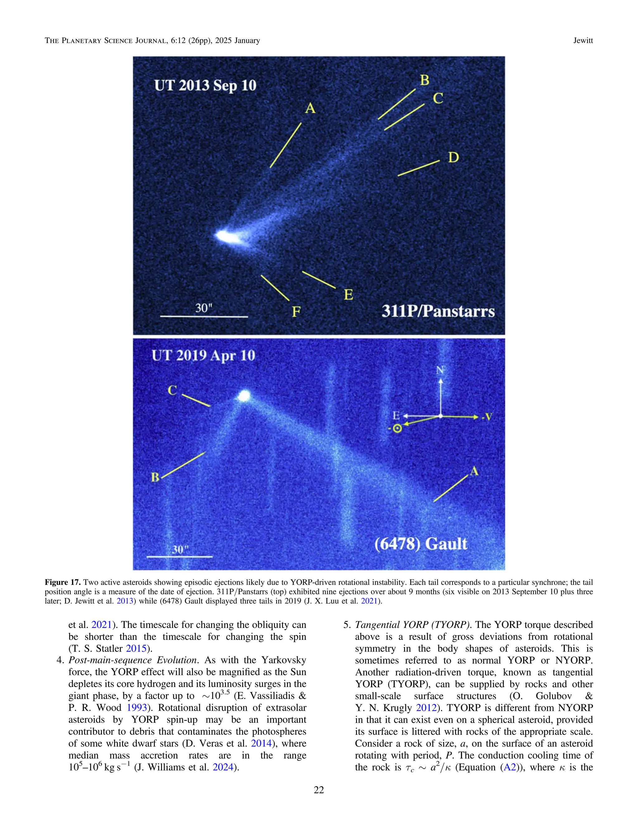

![radii of 1 km and 0.1 km, respectively. The sublimation model
was computed assuming ( )
q
cos = 1/2 in Equation (4), which
lies in between the high- and low-temperature limit models in
Figure 1, and is scaled to timescale τs = 102
yr on a 1 km
nucleus at 1 au, in agreement with the data (Figure 13).
Figure 19 shows that, for a given object size and distances 5
or 6 au, the timescales for spin-change are ∼105
times shorter
for sublimation torques than for YORP torques. Beyond
Saturn, the diminishing water ice sublimation rate pushes the
sublimation timescale to exceed that from YORP, and, in
practice, both processes become so slow in the middle and
outer solar system as to become largely irrelevant.
Acknowledgments
I thank Marco Fenucci for providing a digital table of his
Yarkovsky drift measurements, Pedro Lacerda, Jane Luu, Joe
Masiero, Darryl Seligman, David Vokrouhlicky, Emerson
Whittaker, and an anonymous referee for comments.
Appendix
Thermophysics
To gain some physical insight into how the thermophysical
parameters of an asteroid might affect Yarkovsky and YORP,
we consider the one-dimensional heat conduction equation
( )
r
=
c
T
t
k
T
z
, A1
p
2
2
where T is the temperature, k is the thermal conductivity, ρ is
the bulk density, and cp is the specific heat capacity of the
asteroid surface materials. Dimensionalizing this equation
gives the timescale for heat to conduct over a distance ℓ as
( )
t
k
k
r
~ =
ℓ k
c
where A2
C
p
2
and κ [m2
s−1
] is the thermal diffusivity.4
For a body with
rotation period P, we set τC = P and use Equation (A2) to find
the distance over which heat can conduct in one rotation period
as ℓ = (κP)1/2
, which defines the diurnal thermal skin depth on
the asteroid. An exact solution of Equation (A1) would show
that T varies with depth as a damped sinusoid, with (κP)1/2
being the e-folding length scale of the damping, but our order-
of-magnitude approximation is sufficient here. On a spherical
body with radius a, the heat contained within the skin depth, ℓ,
is
( ) ( )
/
p r k
=
H a P c T
4 A3
p
2 1 2
where cp [J K−1
kg−1
] is the specific heat capacity of the shell.
Loss of heat by radiation into space occurs at the rate
( )
p s
=
dH
dt
a T
4 A4
2 4
where σ = 5.67 × 10⁻⁸
W m−2
K−4
is the Stefan–Boltzmann
radiation constant, and we assume emissivity ε = 1. The order-
Figure 19. The YORP (blue) and water ice sublimation (red) timescales plotted as a function of rH. Timescales for objects 1 km radius (solid lines) and 0.1 km in
radius (dashed lines) are shown. The shaded band marks the approximate location of the main asteroid belt, across which sublimation supplies a ∼105
times stronger
torque if near-surface ice is present.
4
Diffusivity appears directly in Equation (A1) and is the natural measure of
thermal response of a material through Equation (A2). In planetary science, the
use of thermal inertia is instead widely preferred. Thermal inertia is defined by
( ) /
r
=
I k cp
1 2, which has the somewhat uncomfortable units [J m−2
s−1/2
K−1
].
Solid dielectrics (e.g., nonporous rocks) have I ∼ 103
J m−2
s−1/2
K−1
, while
the finest dust, as found in the regoliths of small outer solar system bodies, has
I ∼ 1 to 10 J m−2
s−1/2
K−1
(C. Ferrari 2018). Asteroid inertias in the range 10
„ I „ 100 J m−2
s−1/2
K−1
are common (E. M. MacLennan &
J. P. Emery 2021).
24
The Planetary Science Journal, 6:12 (26pp), 2025 January Jewitt](https://image.slidesharecdn.com/jewitt2025planet-250126132956-3e81e4bc/75/Nongravitational-Forces-in-Planetary-Systems-24-2048.jpg)
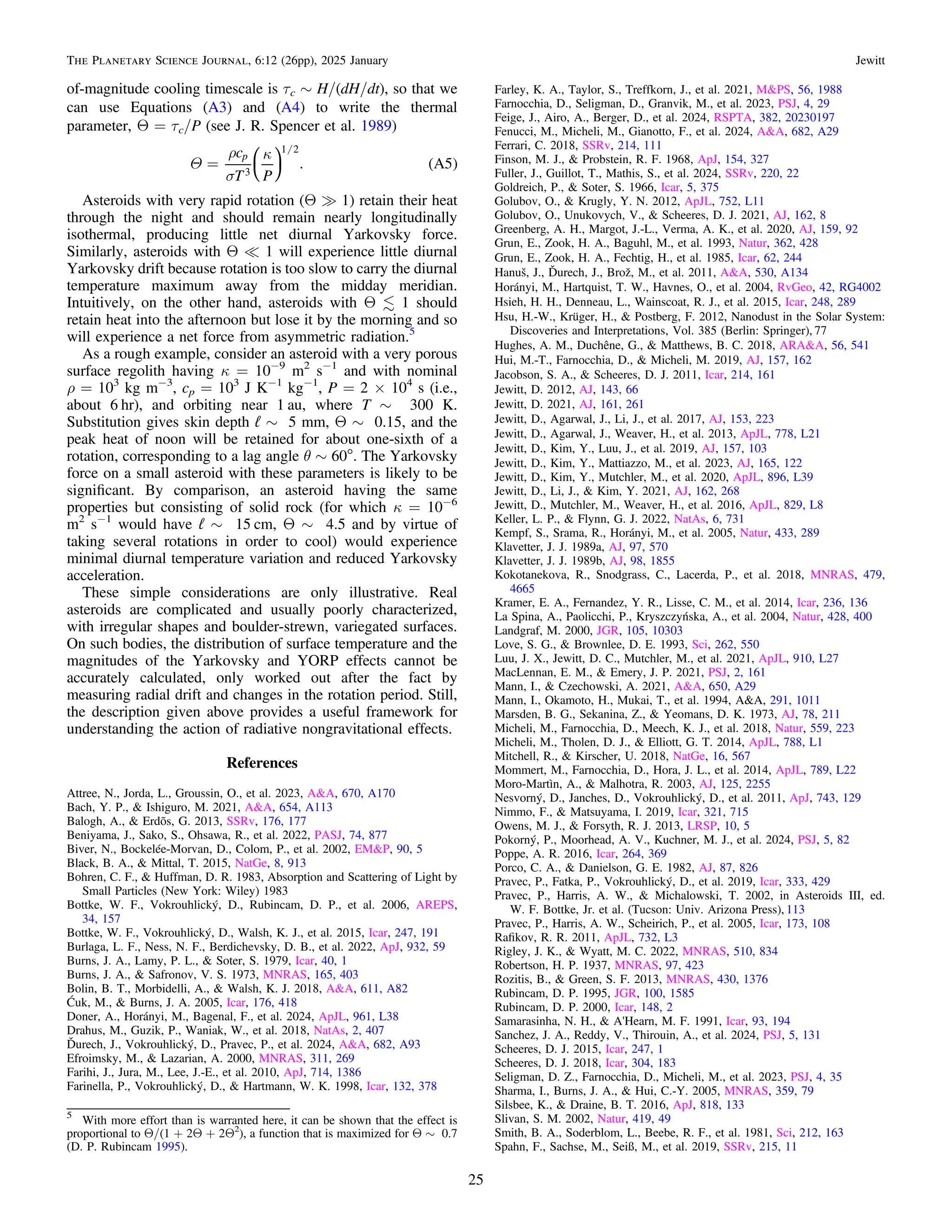

The document discusses the role of nongravitational forces in shaping the dynamics and properties of small planetary bodies in the solar system, including comets, asteroids, and exoplanetary systems. It highlights how these forces, such as sublimation recoil and radiation pressure, are crucial for understanding phenomena that gravity alone cannot explain. The paper aims to simplify the understanding of these complex forces for non-specialists and provides order-of-magnitude descriptions and examples of their applications.


