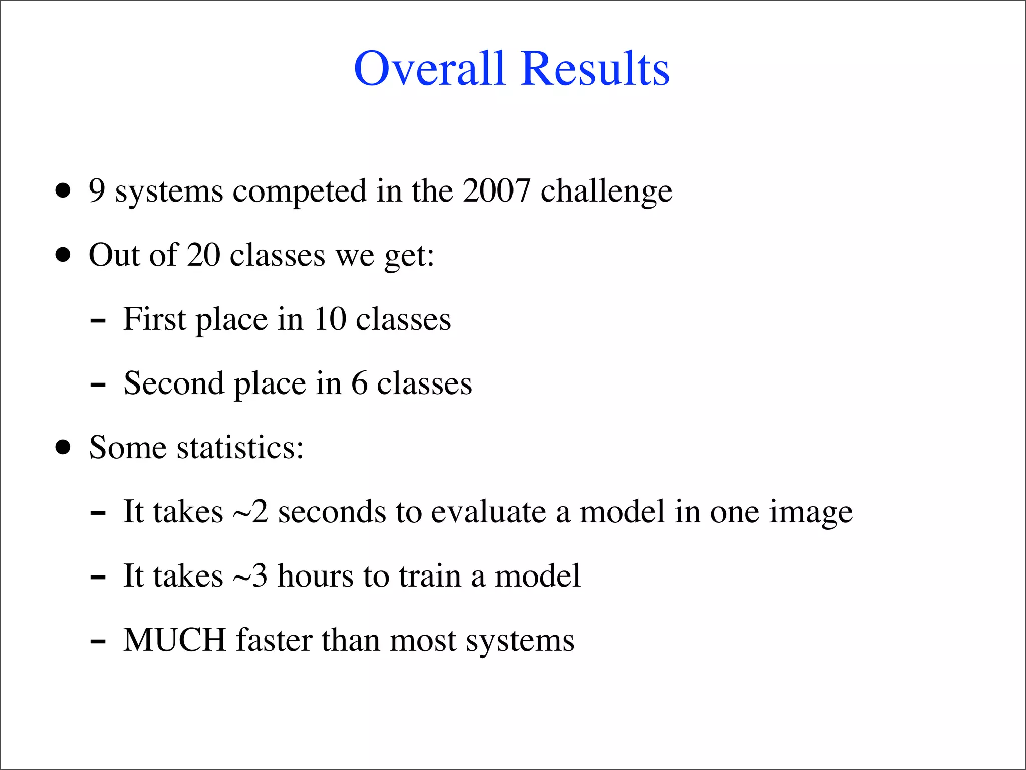
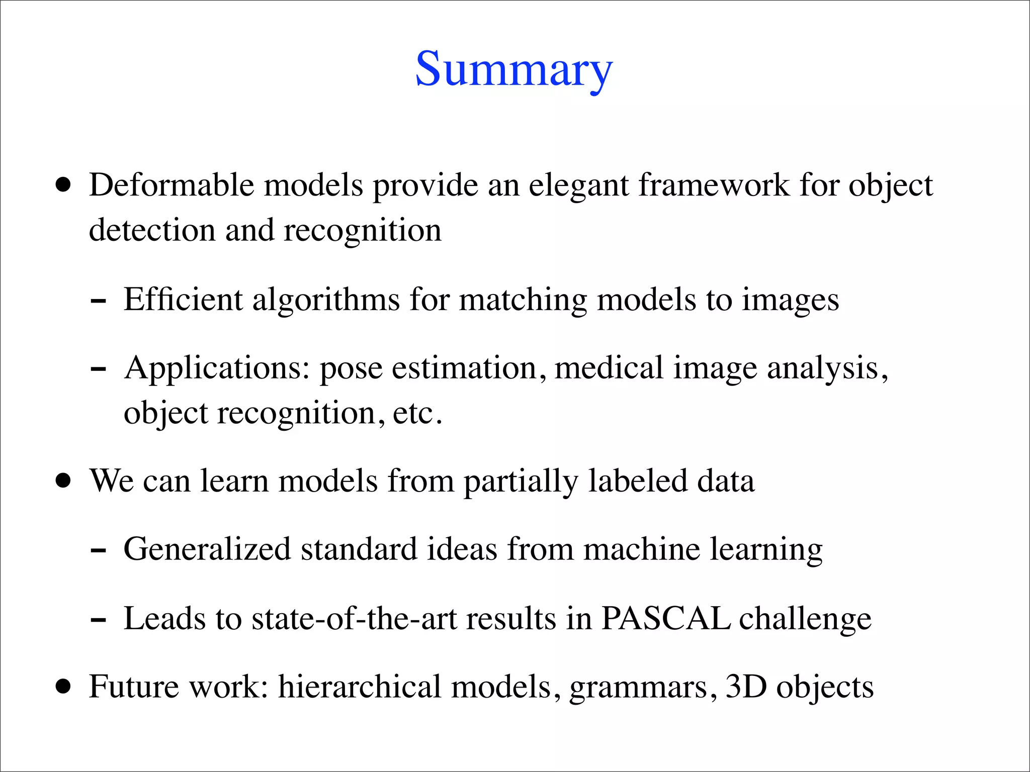
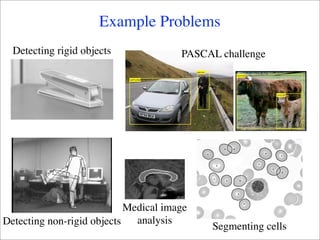
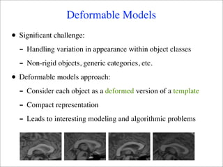
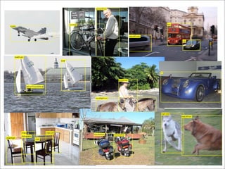
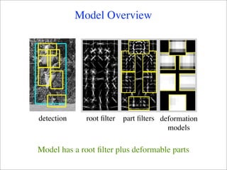
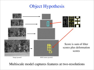
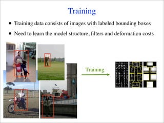
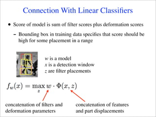
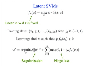
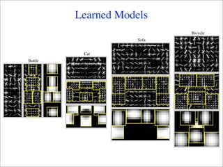
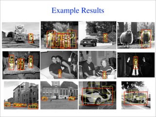
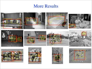
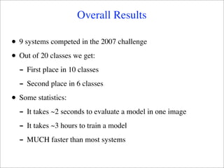
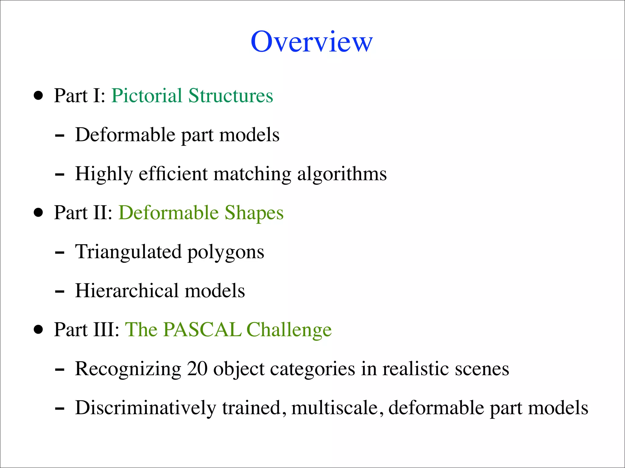
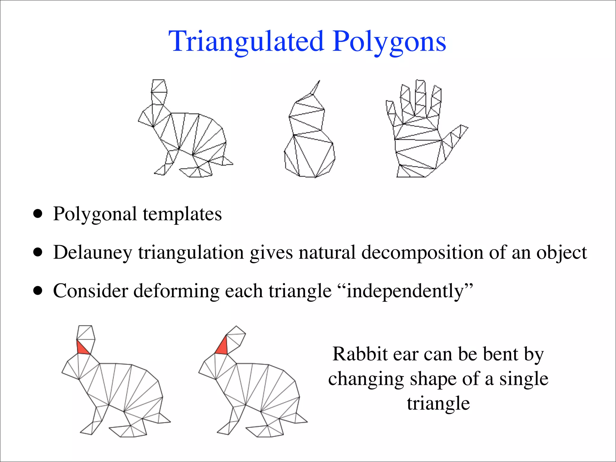
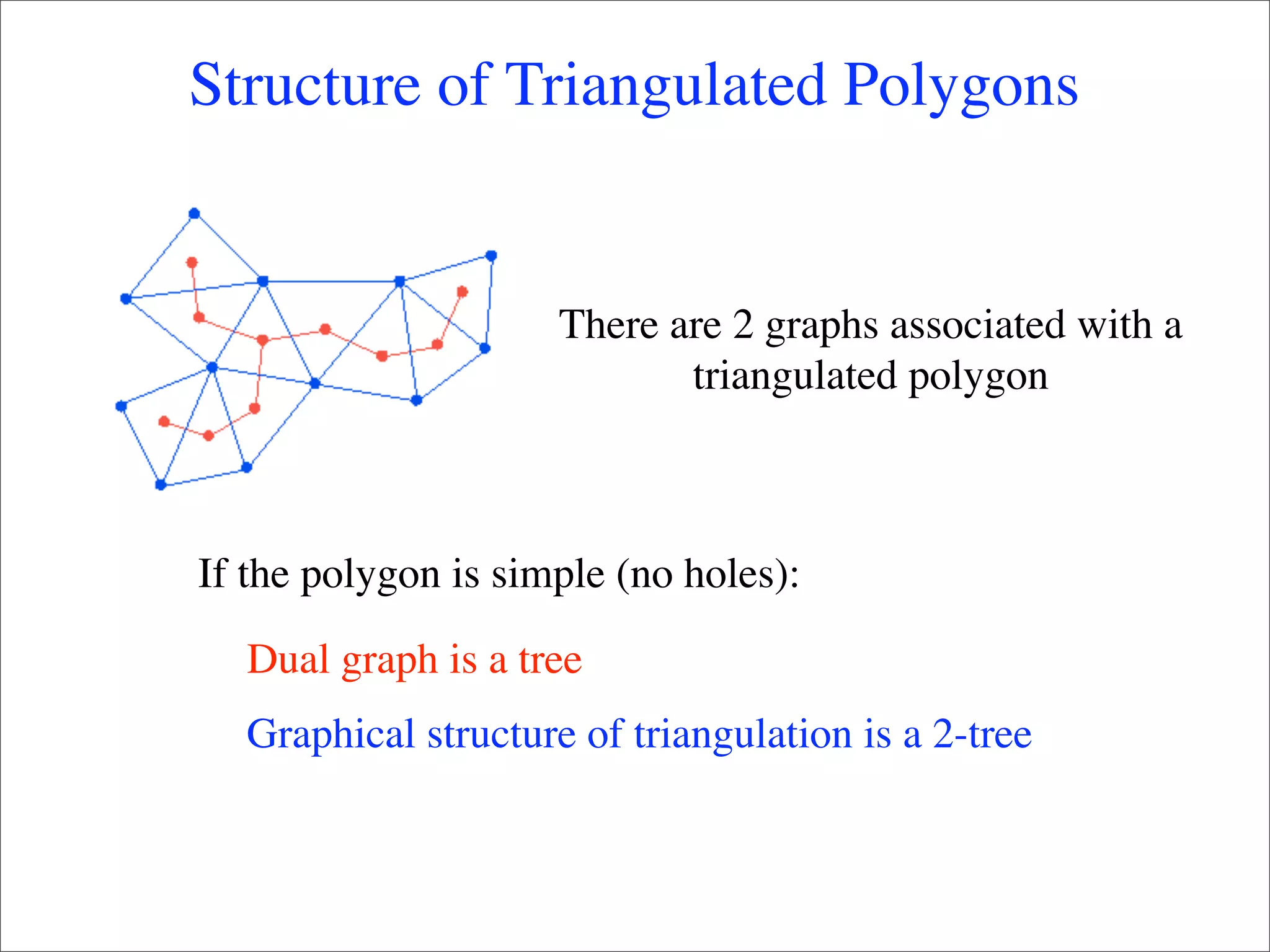
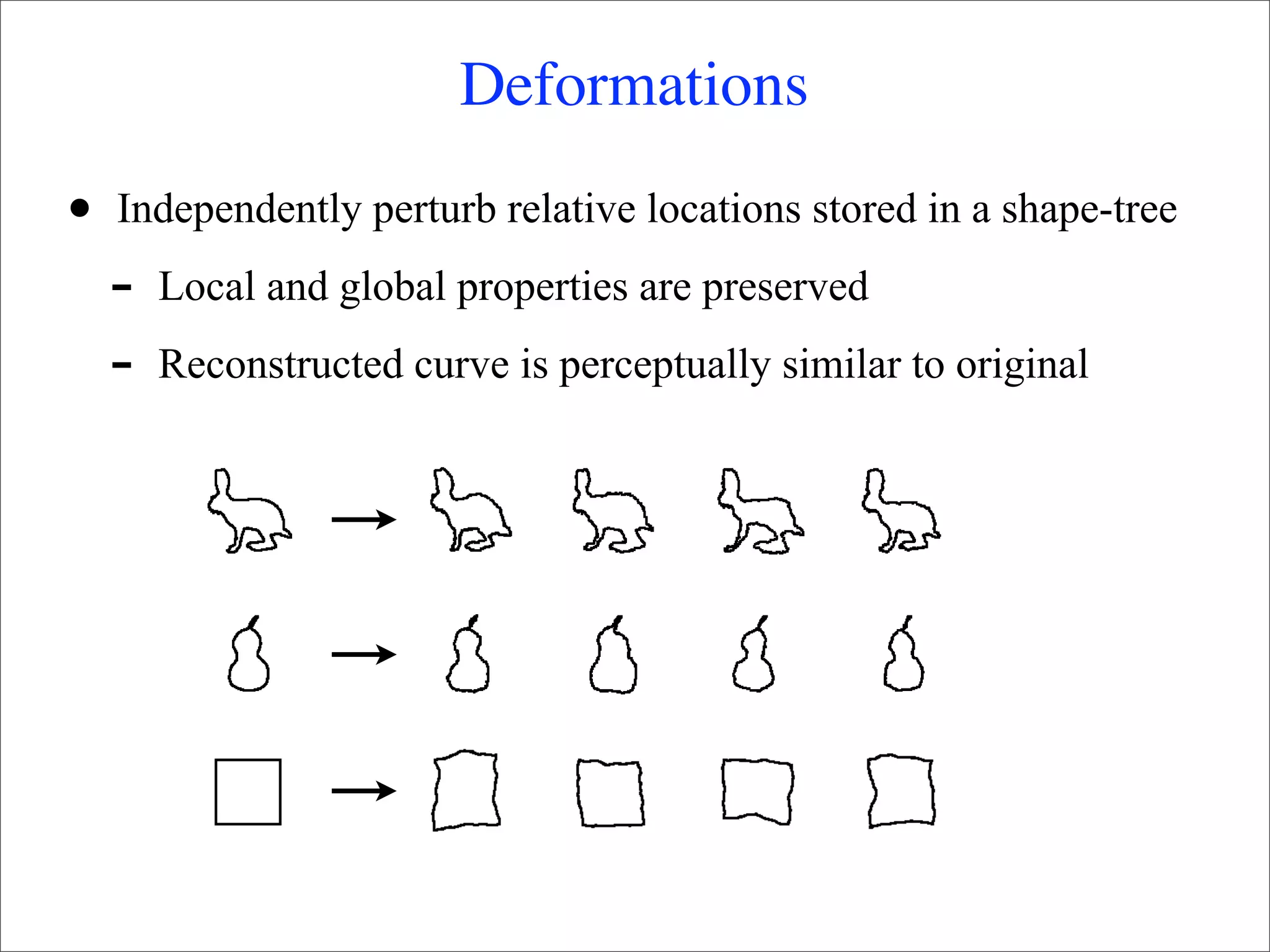
This document summarizes research on using deformable models for object recognition. It discusses using deformable part models to detect objects by optimizing part locations. Efficient algorithms like dynamic programming and min-convolutions are used for matching. Non-rigid objects are modeled using triangulated polygons that can deform individual triangles. Hierarchical shape models capture shape variations. The document applies these techniques to the PASCAL visual object recognition challenge, achieving state-of-the-art results on 10 of 20 object categories through discriminatively trained, multiscale deformable part models.


![Dynamic Programming on Trees
n v2
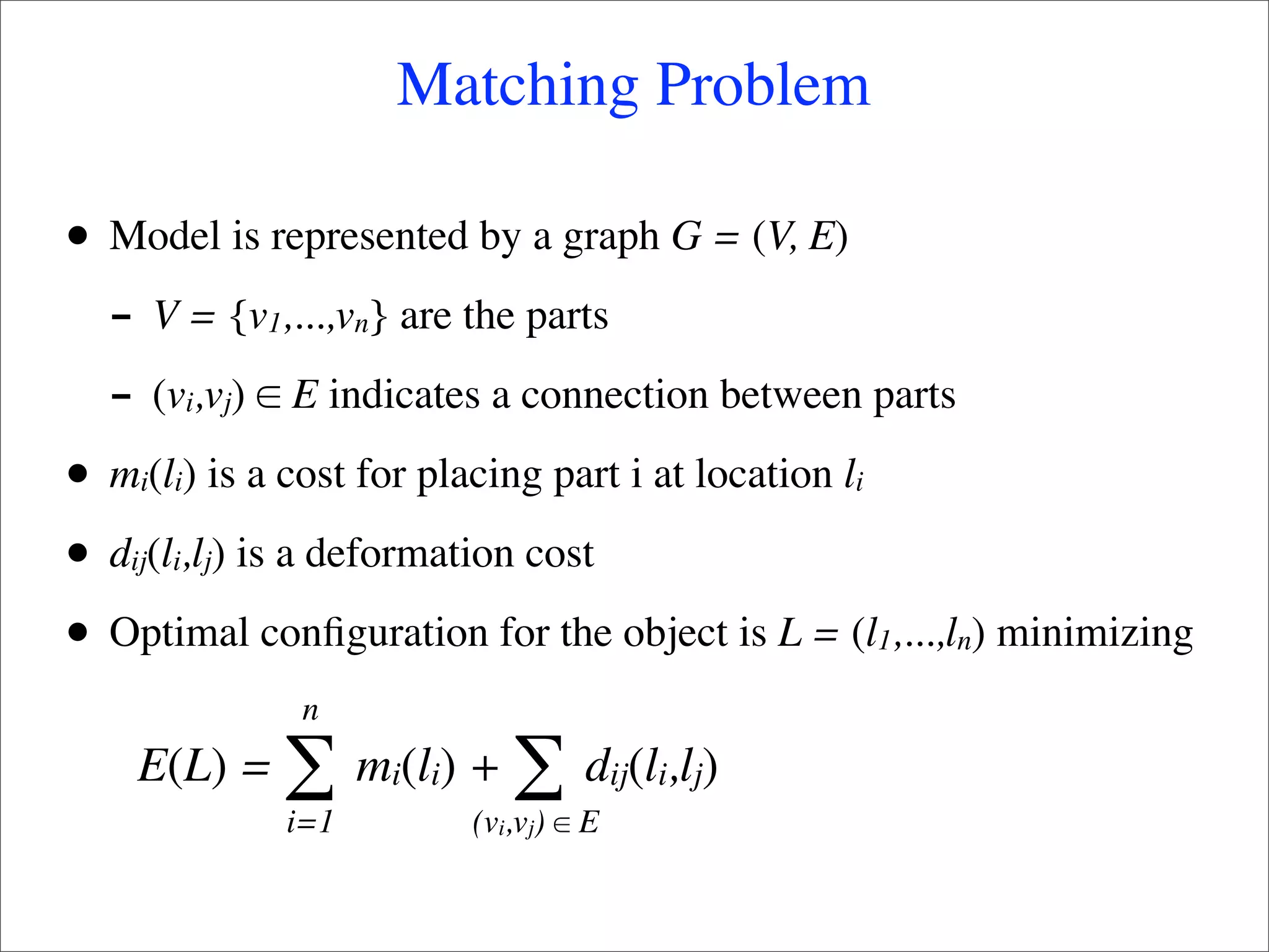
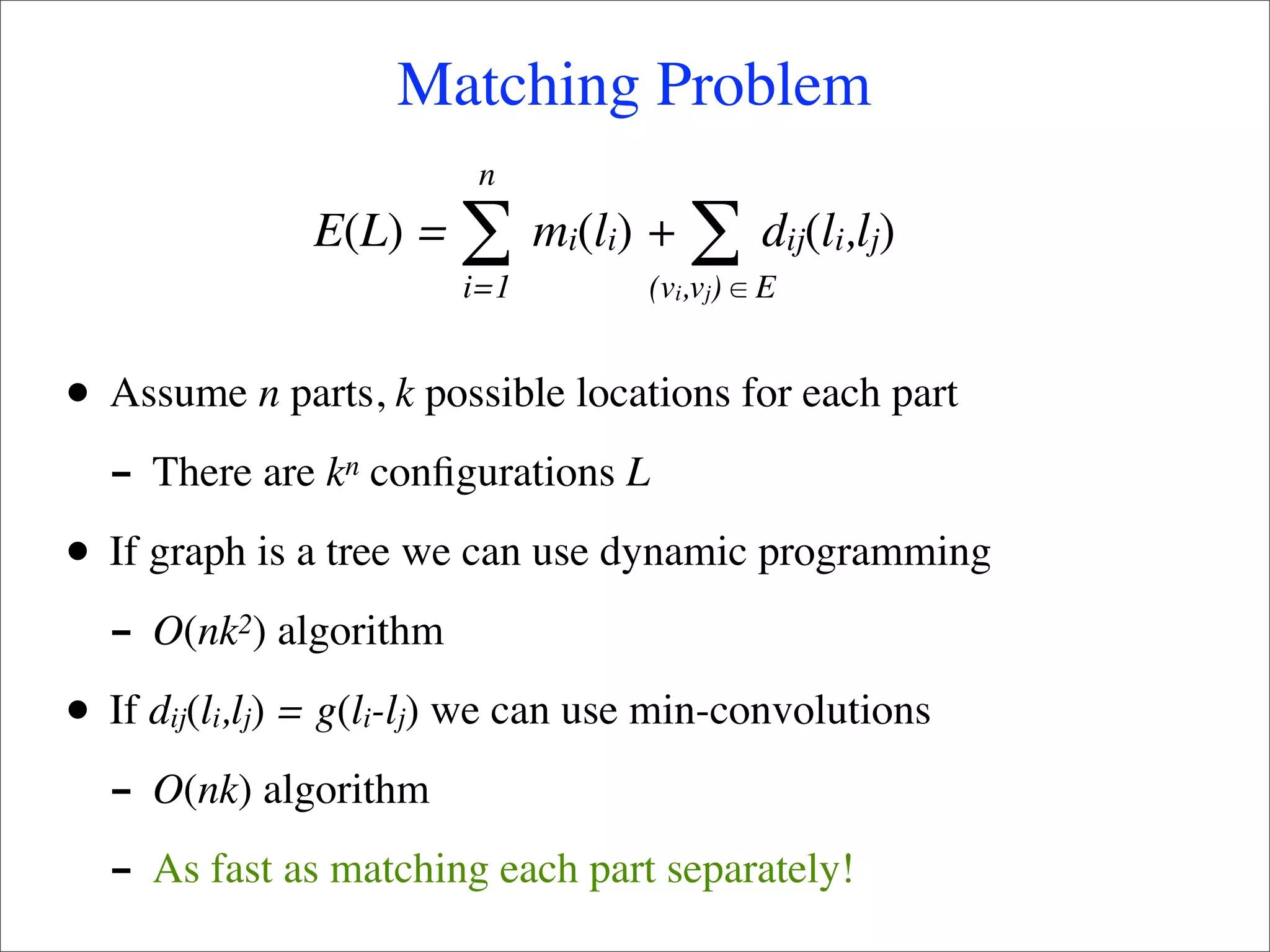
E(L) = ∑ m (l ) + ∑ d (l ,l )
i i ij i j
i=1 (vi,vj) ∈ E v1
• For each l1 find best l2:
- Best (l ) = min [m (l ) + d
2 1
l2
2 2 12(l1,l2) ]
• “Delete” v2 and solve problem with smaller model
• Keep removing leafs until there is a single part left](https://image.slidesharecdn.com/deformable-120208064150-phpapp01/85/Object-Recognition-with-Deformable-Models-9-320.jpg)
![Min-Convolution Speedup
v2
Best2(l1) = min [m2(l2) + d12(l1,l2)] v1
l2
• Brute force: O(k2) --- k is number of locations
• Suppose d12(l1,l2) = g(l1-l2):
- Best (l ) = min [m (l ) + g(l -l )]
2 1
l2
2 2 1 2
• Min-convolution: O(k) if g is convex](https://image.slidesharecdn.com/deformable-120208064150-phpapp01/85/Object-Recognition-with-Deformable-Models-10-320.jpg)


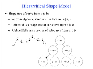
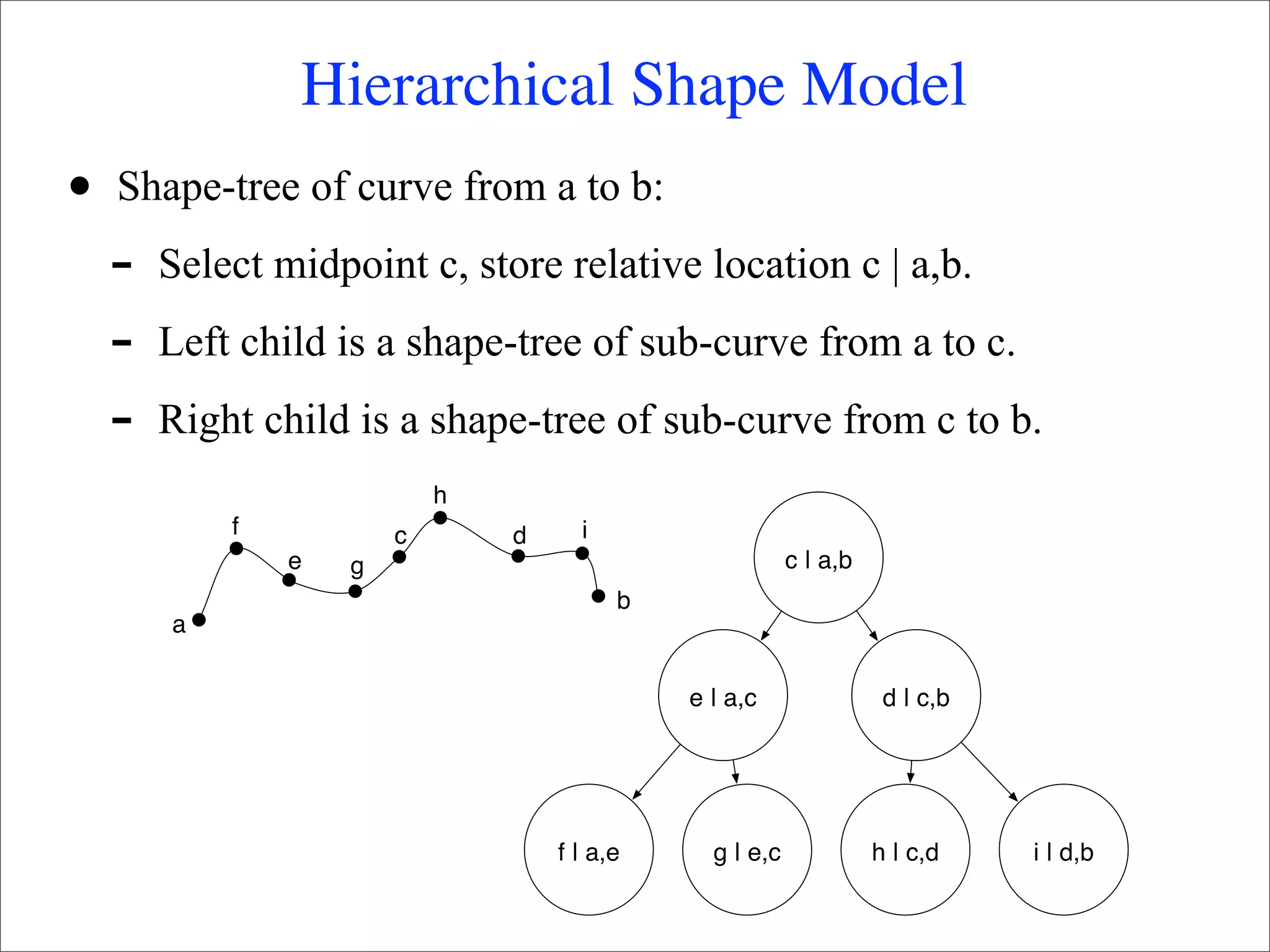
![Matching
h
f c d i
e g c | a,b
a
b w p
e | a,c d | c,b
r
v f | a,e g | e,c h | c,d i | d,b
q
u
model curve
Match(v, [p,q]) = w1
Match(u, [q,r]) = w2
Match(w, [p,r]) = w1 + w2 + dif((e|a,c), (q|p,r))
similar to parsing with the CKY algorithm](https://image.slidesharecdn.com/deformable-120208064150-phpapp01/85/Object-Recognition-with-Deformable-Models-20-320.jpg)


![Dynamic Programming on Trees
n v2
E(L) = ∑ m (l ) + ∑ d (l ,l )
i i ij i j
i=1 (vi,vj) ∈ E v1
• For each l1 find best l2:
- Best (l ) = min [m (l ) + d
2 1
l2
2 2 12(l1,l2) ]
• “Delete” v2 and solve problem with smaller model
• Keep removing leafs until there is a single part left](https://image.slidesharecdn.com/deformable-120208064150-phpapp01/75/Object-Recognition-with-Deformable-Models-9-2048.jpg)
![Min-Convolution Speedup
v2
Best2(l1) = min [m2(l2) + d12(l1,l2)] v1
l2
• Brute force: O(k2) --- k is number of locations
• Suppose d12(l1,l2) = g(l1-l2):
- Best (l ) = min [m (l ) + g(l -l )]
2 1
l2
2 2 1 2
• Min-convolution: O(k) if g is convex](https://image.slidesharecdn.com/deformable-120208064150-phpapp01/75/Object-Recognition-with-Deformable-Models-10-2048.jpg)

![Matching
h
f c d i
e g c | a,b
a
b w p
e | a,c d | c,b
r
v f | a,e g | e,c h | c,d i | d,b
q
u
model curve
Match(v, [p,q]) = w1
Match(u, [q,r]) = w2
Match(w, [p,r]) = w1 + w2 + dif((e|a,c), (q|p,r))
similar to parsing with the CKY algorithm](https://image.slidesharecdn.com/deformable-120208064150-phpapp01/75/Object-Recognition-with-Deformable-Models-20-2048.jpg)