Download as PDF, PPTX


![Local minima
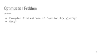
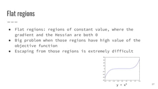
● In practice, local minima is not a major problem
● [1] gives some theoretical insights about local minima:
○ For large-size networks, most local minima are equivalent and yield
similar performance on a test set
○ The probability of finding a “bad” (high value) local minimum is
non-zero for small-size networks and decreases quickly with network
size
○ Struggling to find the global minimum on the training set (as opposed
to one of the many good local ones) is not useful in practice and may
lead to overfitting
25[1] Choromanska et al. 2014.](https://image.slidesharecdn.com/optimizationalgorithms-170625041750/85/Overview-on-Optimization-algorithms-in-Deep-Learning-25-320.jpg)
![Saddle points
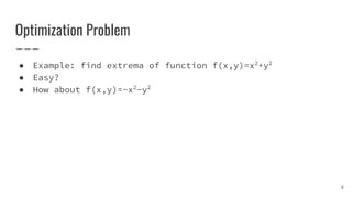
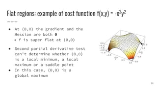
● For high-dimensional non-convex functions, saddle points
are much more than local minima (and maxima) [1]
● Saddle points slow down training process
○ Batch Gradient Descent may be stuck at saddle points
○ Stochastic Gradient Descent seems to be able to escape saddle points
in many cases [2]
26
[1] Dauphin et al. 2014.
[2] Goodfellow et al. 2015.](https://image.slidesharecdn.com/optimizationalgorithms-170625041750/85/Overview-on-Optimization-algorithms-in-Deep-Learning-26-320.jpg)


![Machine Learning Definition
"A computer program is said to learn from experience E with
respect to some class of tasks T and performance measure P
if its performance at tasks in T, as measured by P, improves
with experience E." [1]
[1] Mitchell, T. (1997). Machine Learning. McGraw Hill. p2.
44](https://image.slidesharecdn.com/optimizationalgorithms-170625041750/85/Overview-on-Optimization-algorithms-in-Deep-Learning-44-320.jpg)

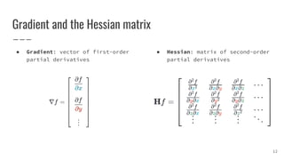
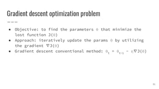
![Sharp and Wide Minima [1]
● Large-batch Gradient Descent tends to converge to sharp minima
→ poorer generalization
● Small-batch Gradient Descent consistently converges to wide minima
→ better generalization
47[1] Keskar et al. 2017.](https://image.slidesharecdn.com/optimizationalgorithms-170625041750/85/Overview-on-Optimization-algorithms-in-Deep-Learning-47-320.jpg)


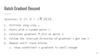
![Local minima
● In practice, local minima is not a major problem
● [1] gives some theoretical insights about local minima:
○ For large-size networks, most local minima are equivalent and yield
similar performance on a test set
○ The probability of finding a “bad” (high value) local minimum is
non-zero for small-size networks and decreases quickly with network
size
○ Struggling to find the global minimum on the training set (as opposed
to one of the many good local ones) is not useful in practice and may
lead to overfitting
25[1] Choromanska et al. 2014.](https://image.slidesharecdn.com/optimizationalgorithms-170625041750/75/Overview-on-Optimization-algorithms-in-Deep-Learning-25-2048.jpg)
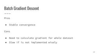
![Saddle points
● For high-dimensional non-convex functions, saddle points
are much more than local minima (and maxima) [1]
● Saddle points slow down training process
○ Batch Gradient Descent may be stuck at saddle points
○ Stochastic Gradient Descent seems to be able to escape saddle points
in many cases [2]
26
[1] Dauphin et al. 2014.
[2] Goodfellow et al. 2015.](https://image.slidesharecdn.com/optimizationalgorithms-170625041750/75/Overview-on-Optimization-algorithms-in-Deep-Learning-26-2048.jpg)


![Machine Learning Definition
"A computer program is said to learn from experience E with
respect to some class of tasks T and performance measure P
if its performance at tasks in T, as measured by P, improves
with experience E." [1]
[1] Mitchell, T. (1997). Machine Learning. McGraw Hill. p2.
44](https://image.slidesharecdn.com/optimizationalgorithms-170625041750/75/Overview-on-Optimization-algorithms-in-Deep-Learning-44-2048.jpg)

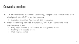
![Sharp and Wide Minima [1]
● Large-batch Gradient Descent tends to converge to sharp minima
→ poorer generalization
● Small-batch Gradient Descent consistently converges to wide minima
→ better generalization
47[1] Keskar et al. 2017.](https://image.slidesharecdn.com/optimizationalgorithms-170625041750/75/Overview-on-Optimization-algorithms-in-Deep-Learning-47-2048.jpg)

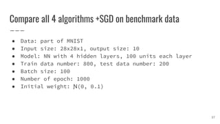
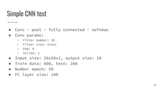
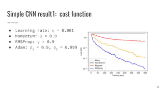
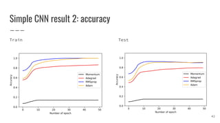
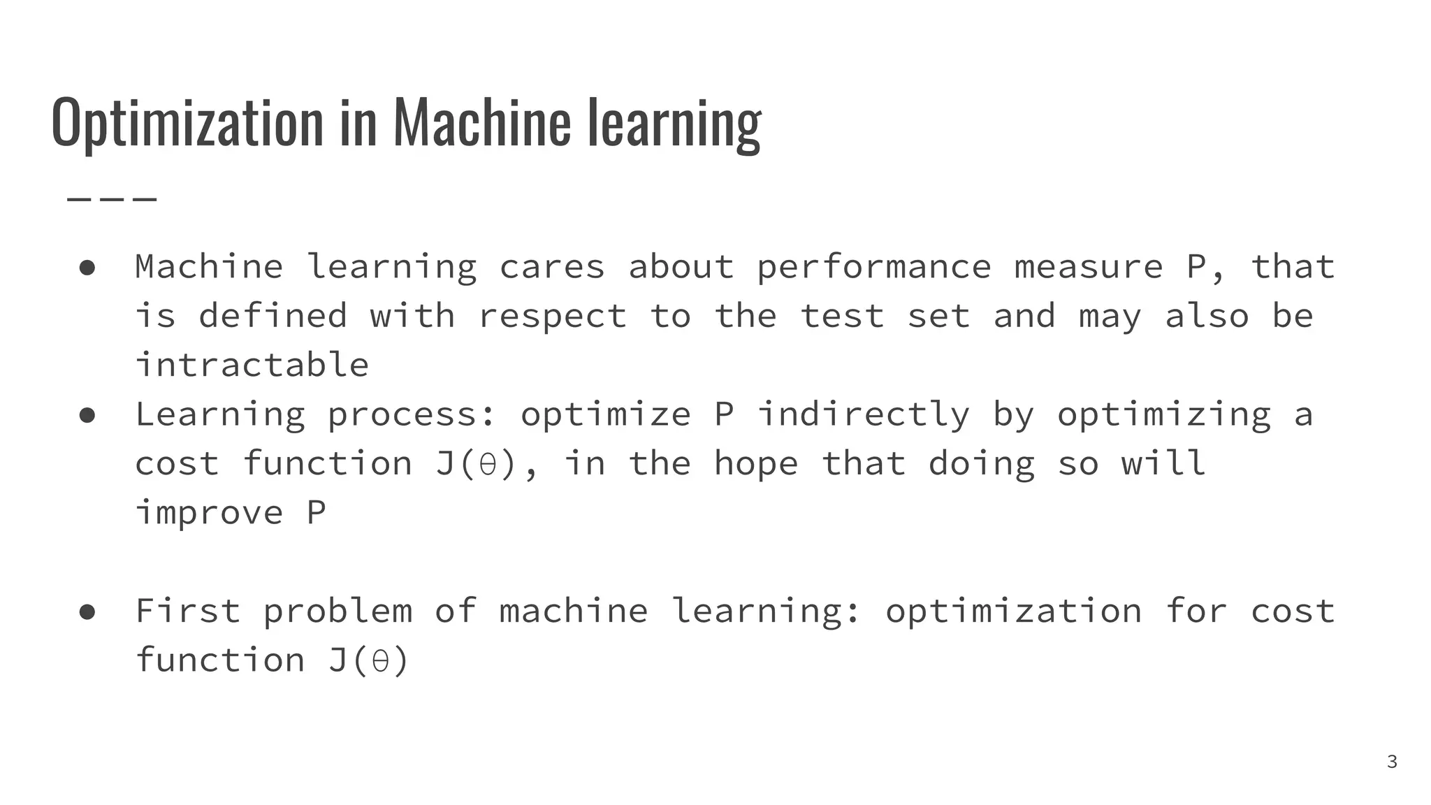
The document covers gradient descent optimization algorithms, focusing on their application in machine learning and the challenges encountered, such as local minima, saddle points, and flat regions. It details various optimization techniques, including batch and stochastic gradient descent, as well as advanced methods like momentum and adaptive learning rates. Additionally, it presents comparative results of these algorithms on benchmark data for training and accuracy of a neural network model.
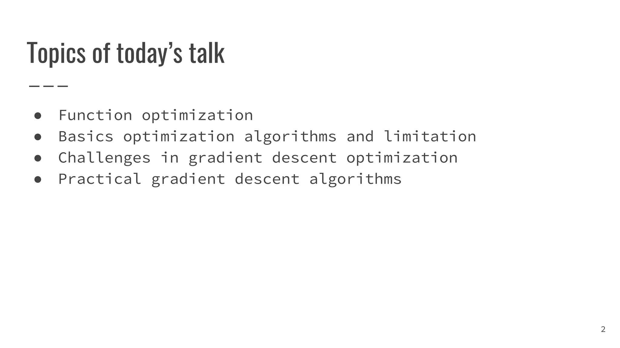
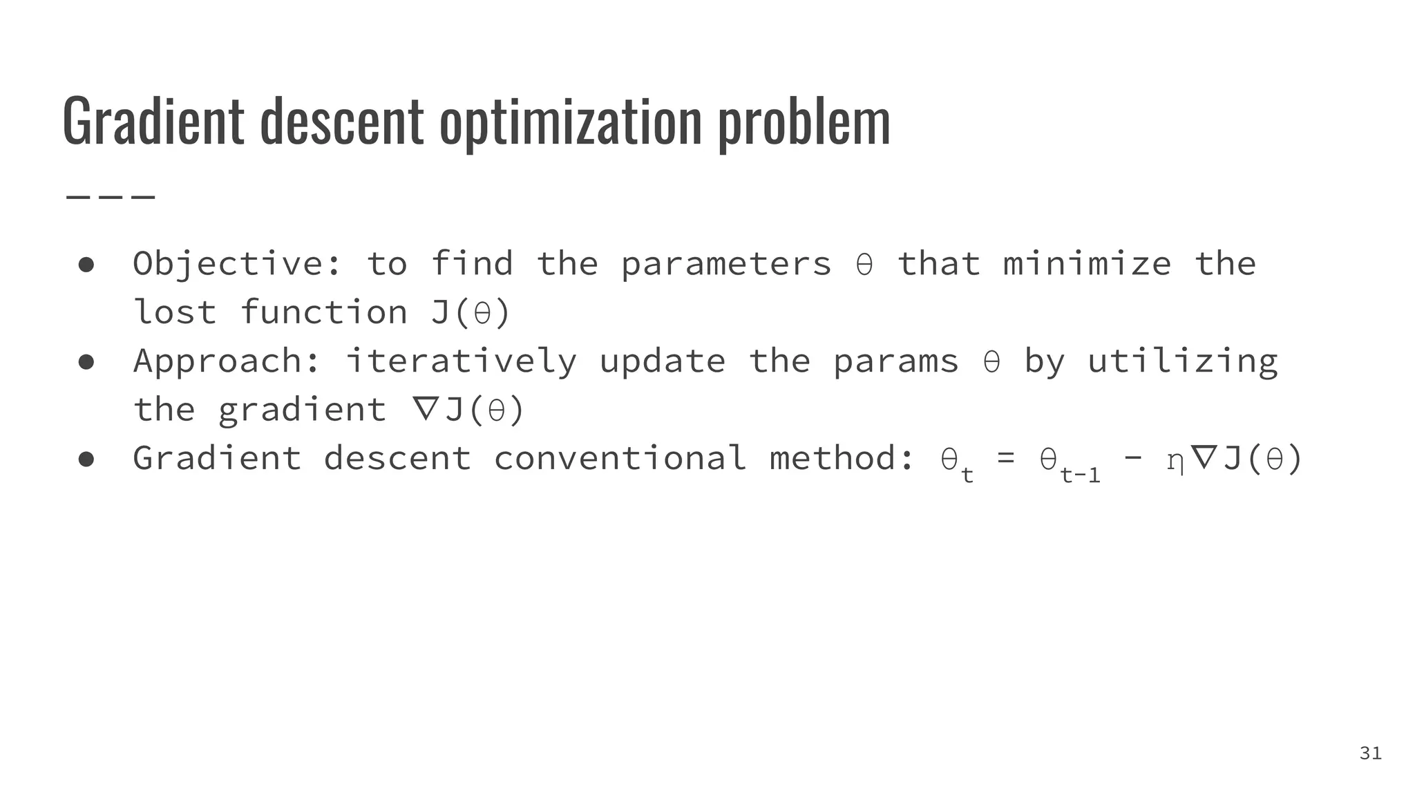
Introduction to gradient descent optimization, today’s talk on function optimization and algorithm challenges.
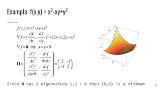
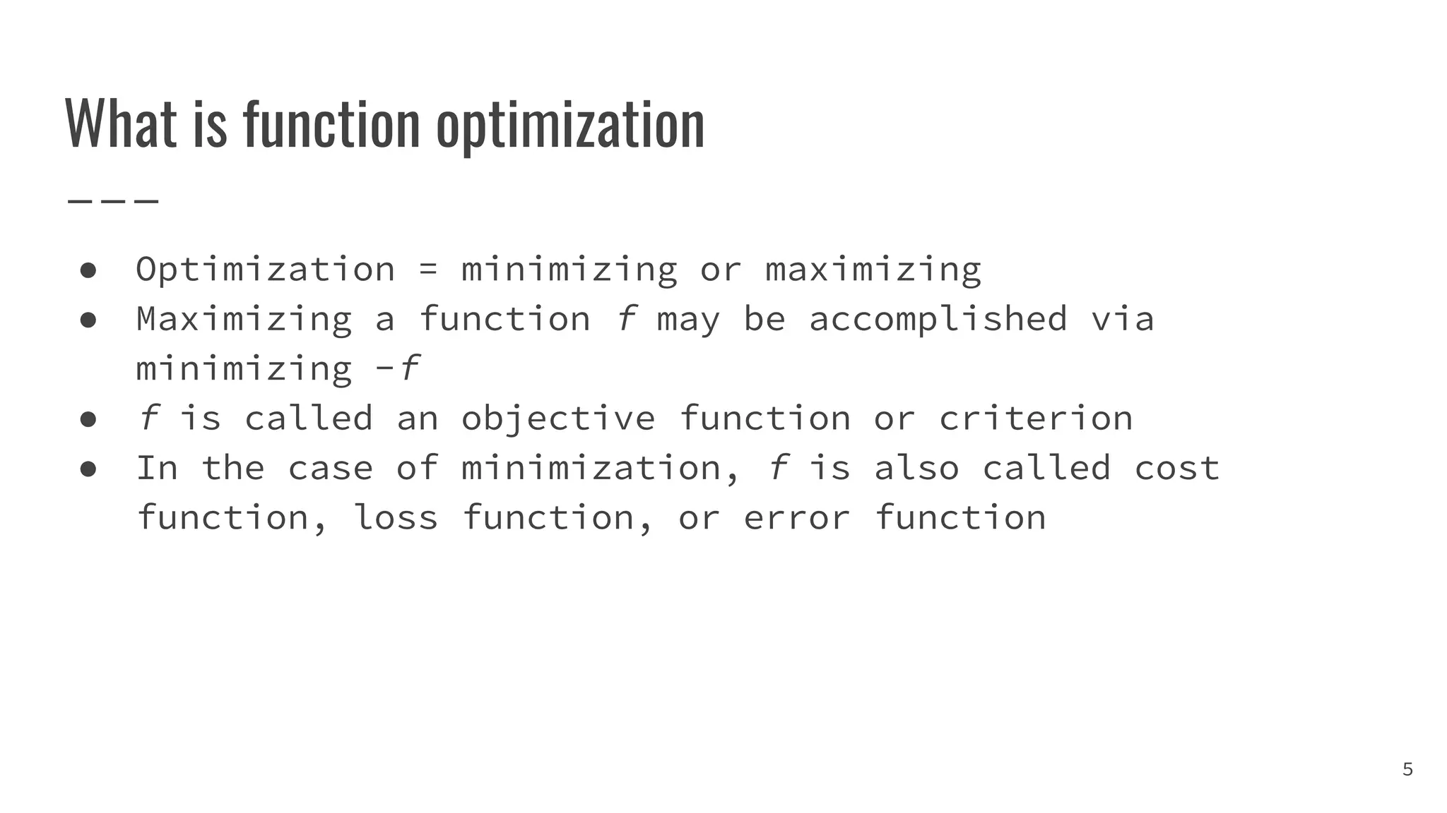
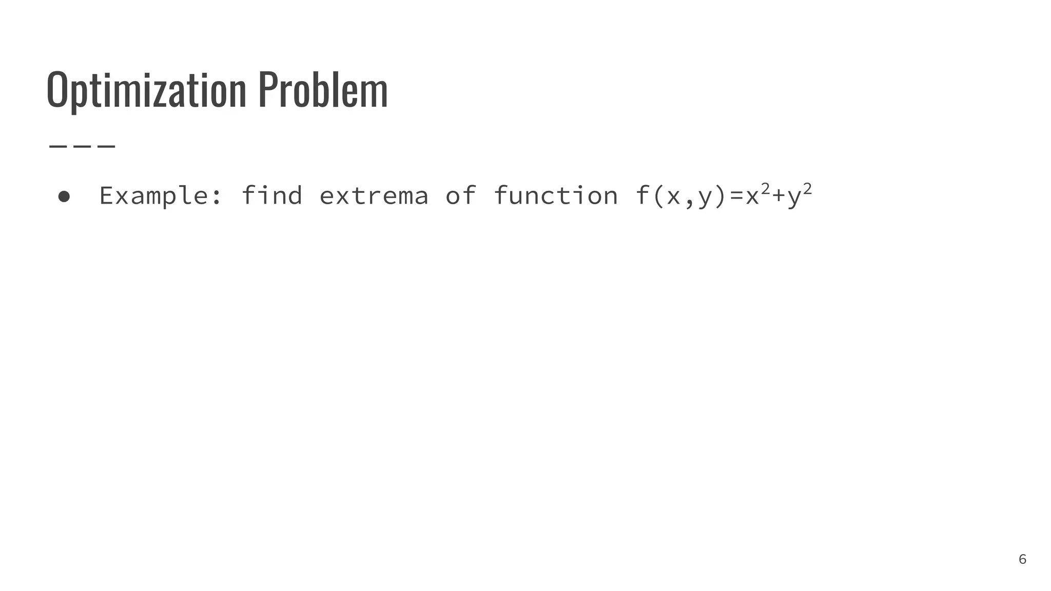
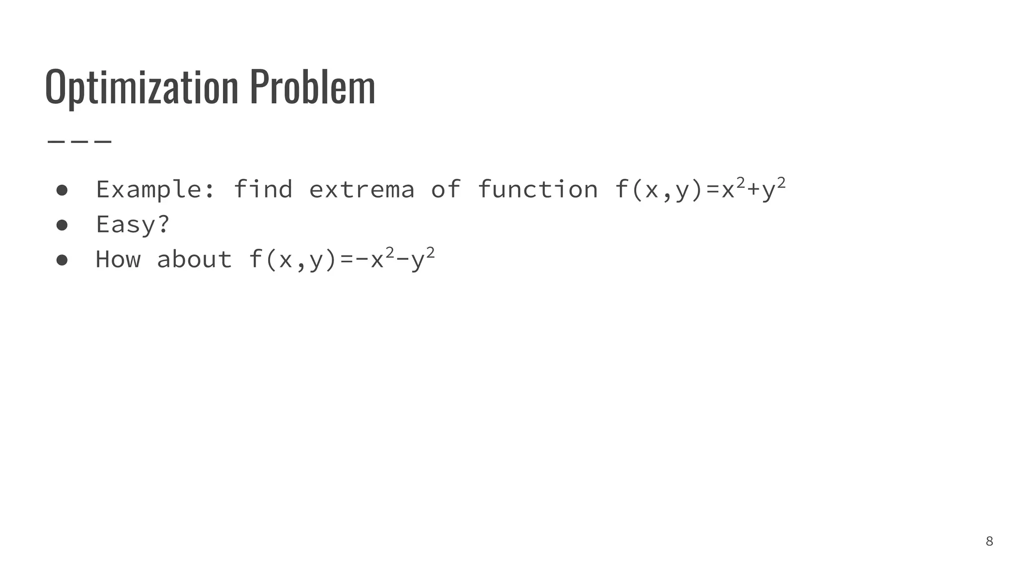
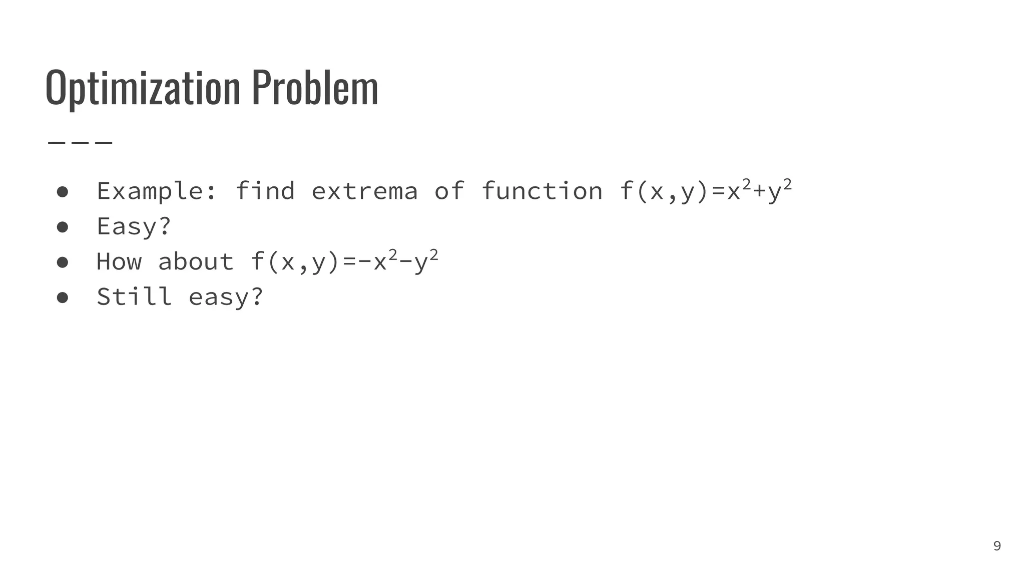
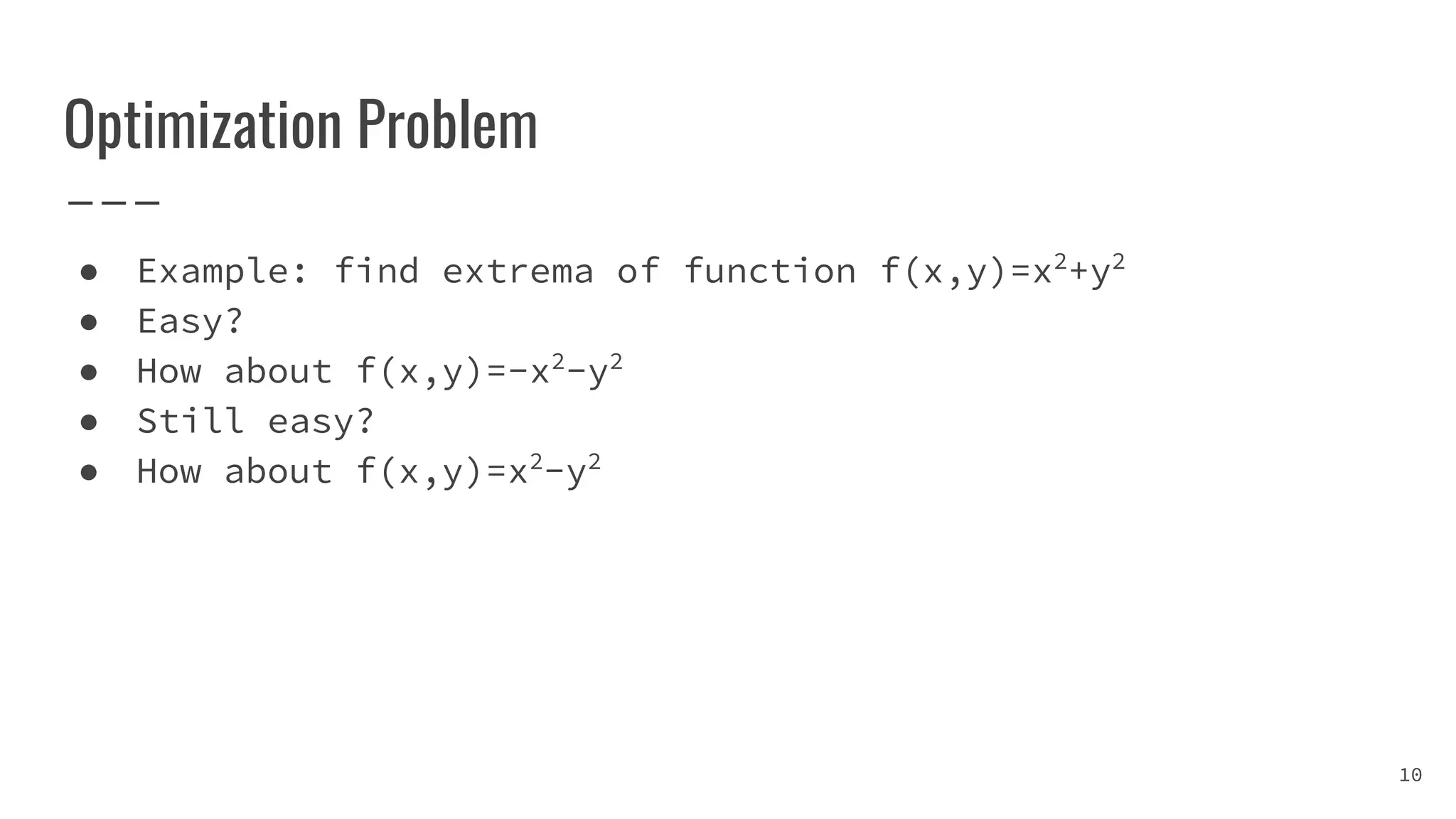
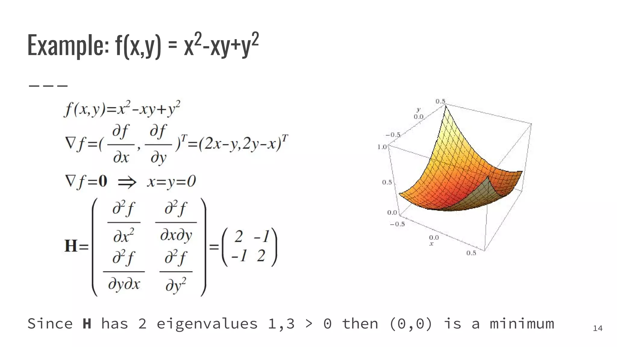
Definition and examples of function optimization, including mathematical expressions for finding extrema.
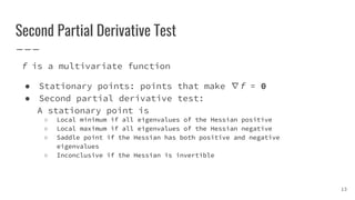
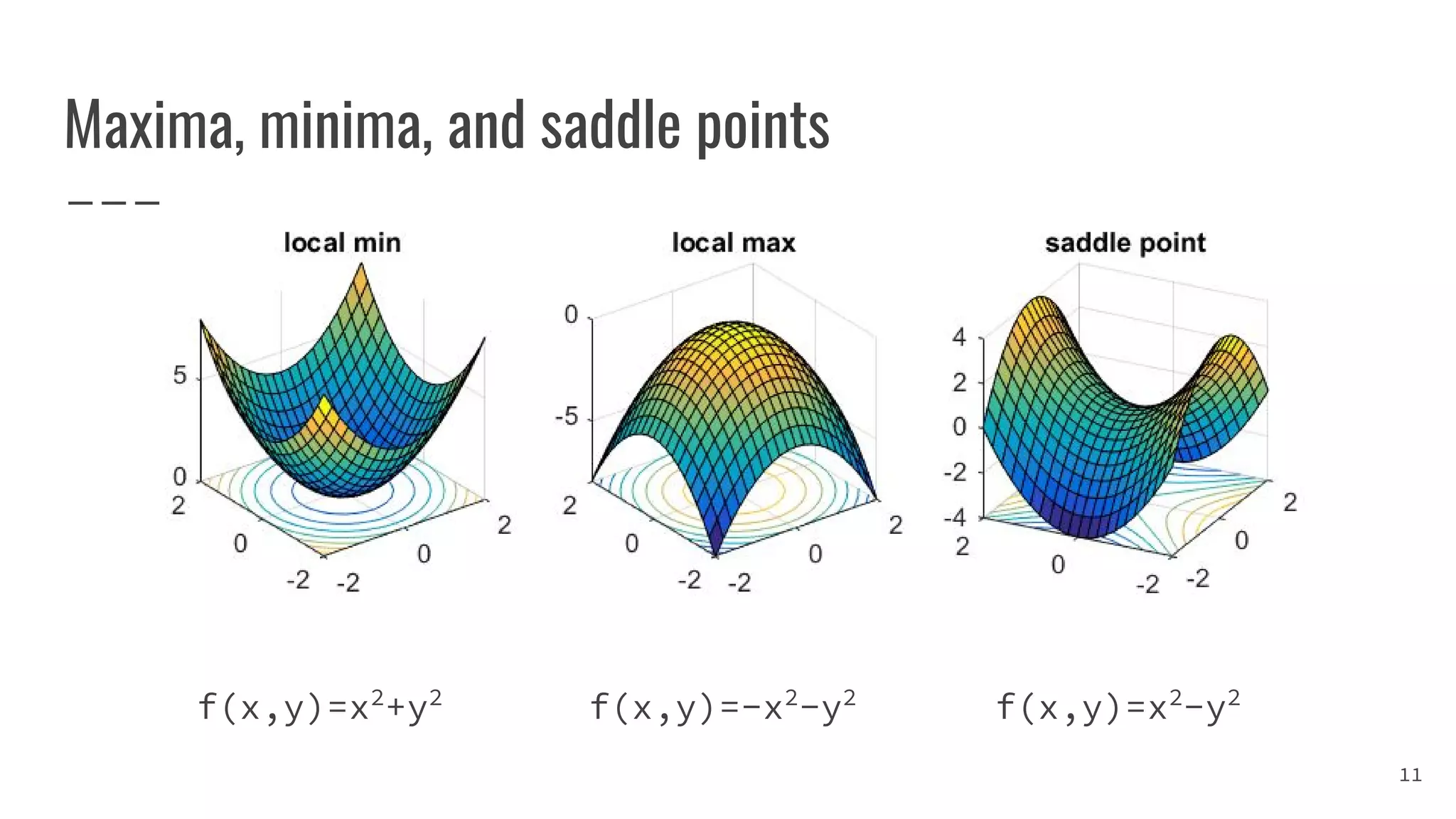
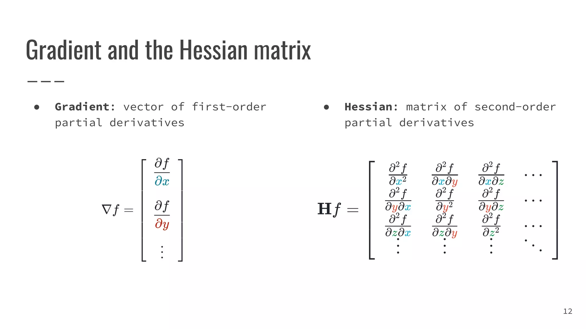
Explains maxima, minima, saddle points, gradients, and Hessian matrix for multivariate functions.
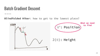
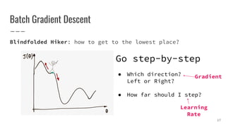
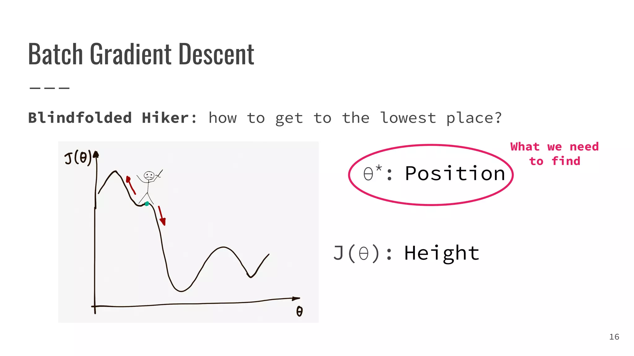
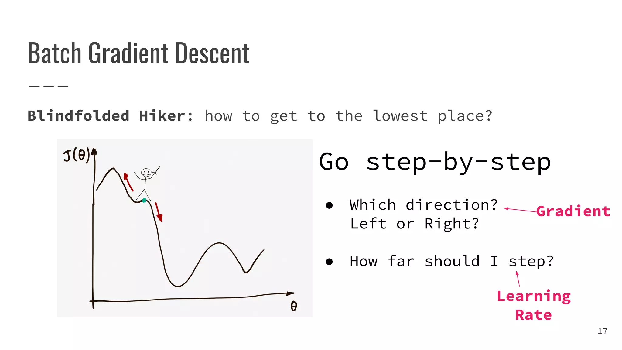
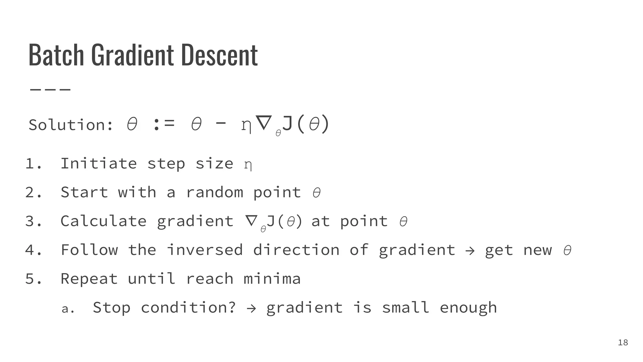
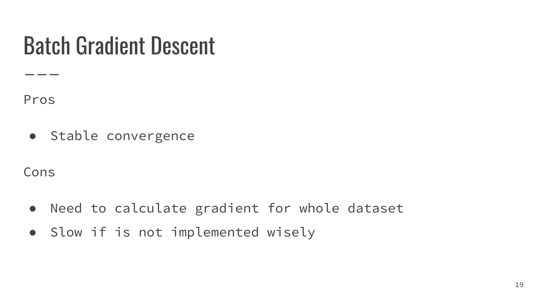
Introduction to batch gradient descent including its advantages, disadvantages, and steps.
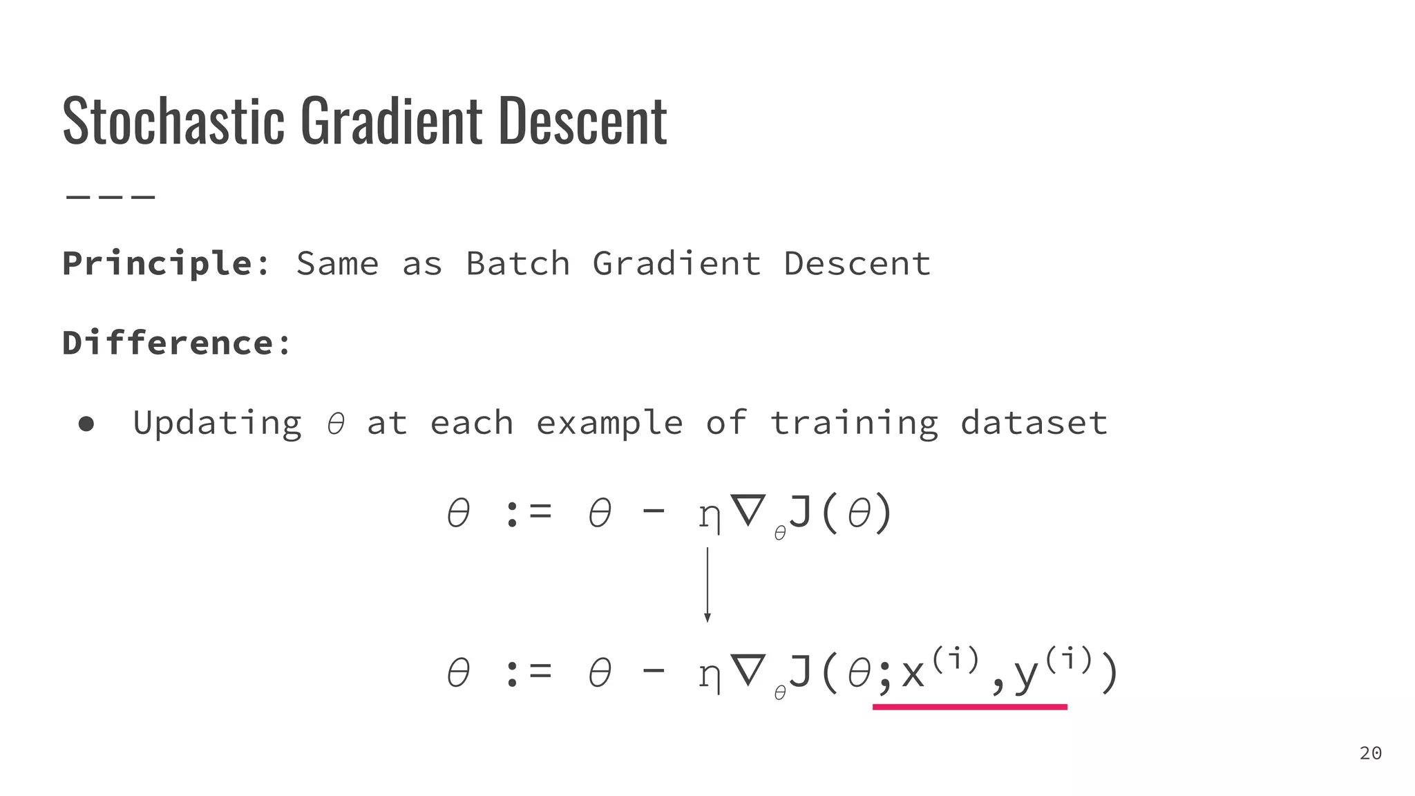
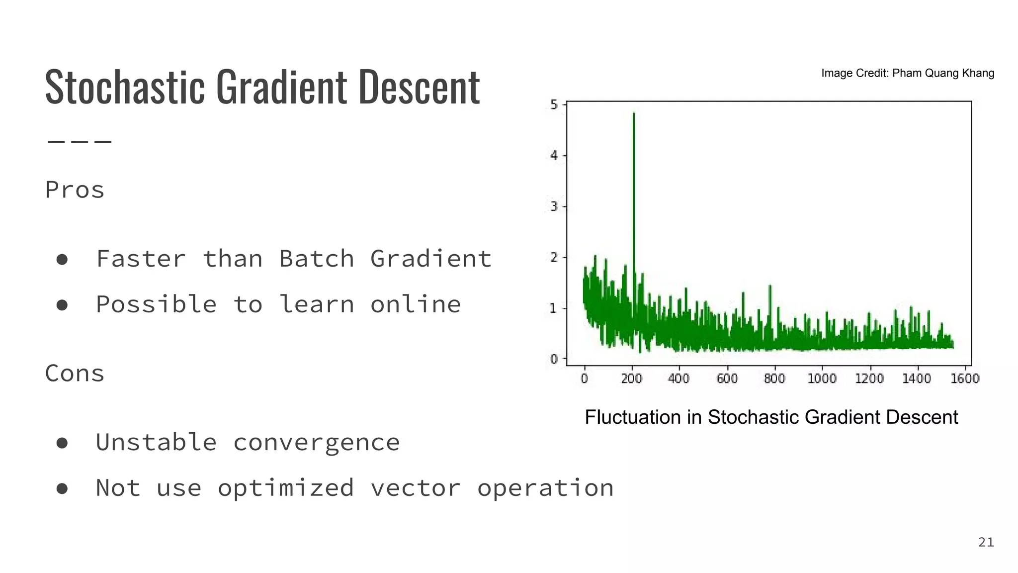
Principles of stochastic gradient descent, differences from batch gradient descent, pros and cons.
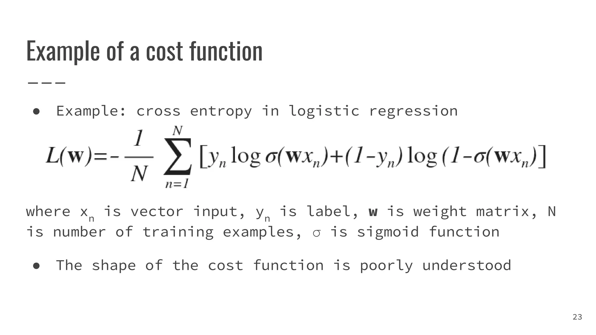
Discusses examples of cost functions, convexity problems, and challenges with local minima and saddle points.
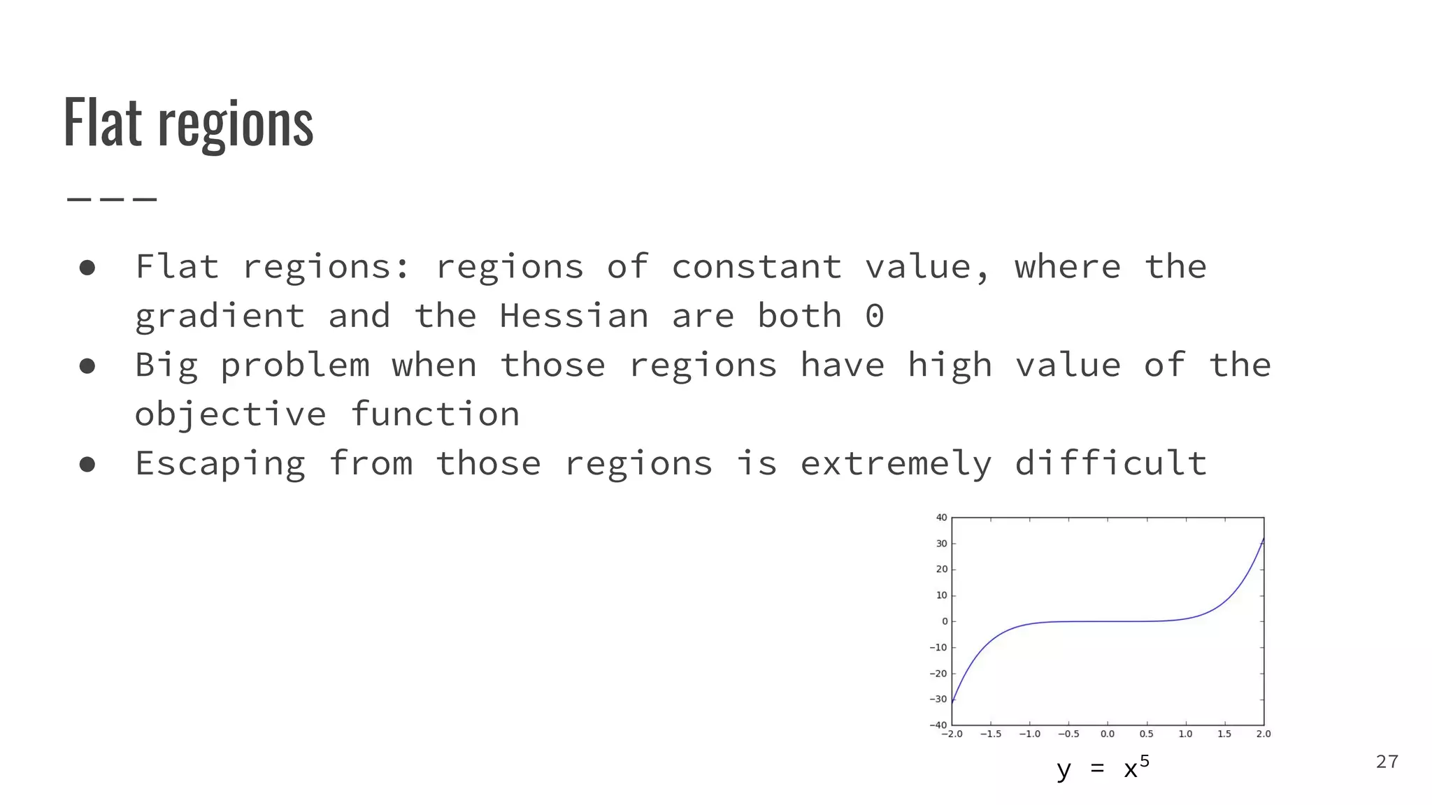
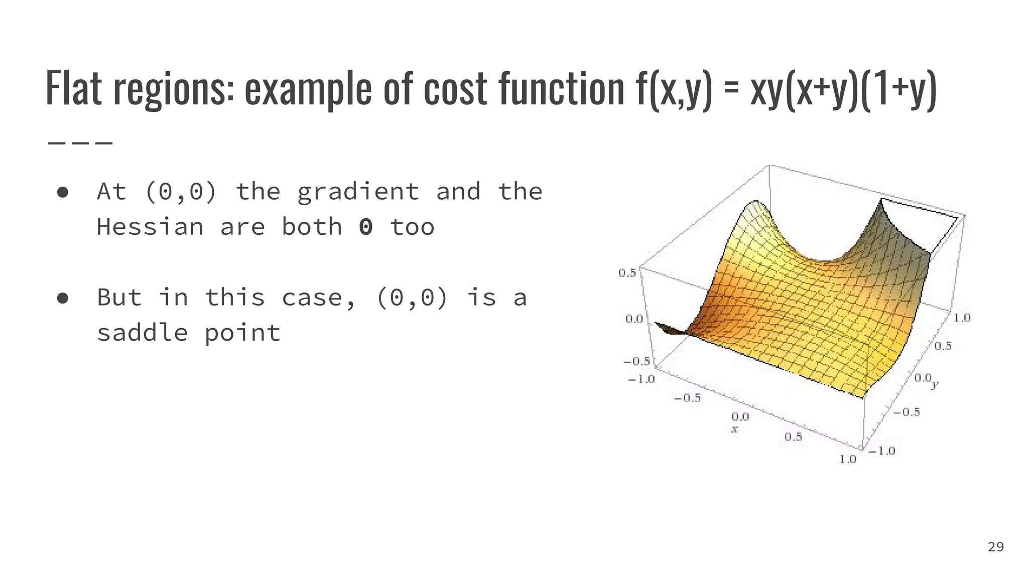
Describes flat regions in optimization landscapes that pose challenges for convergence.
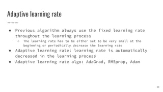
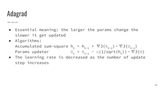
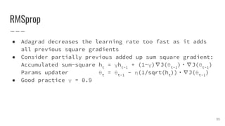
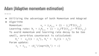
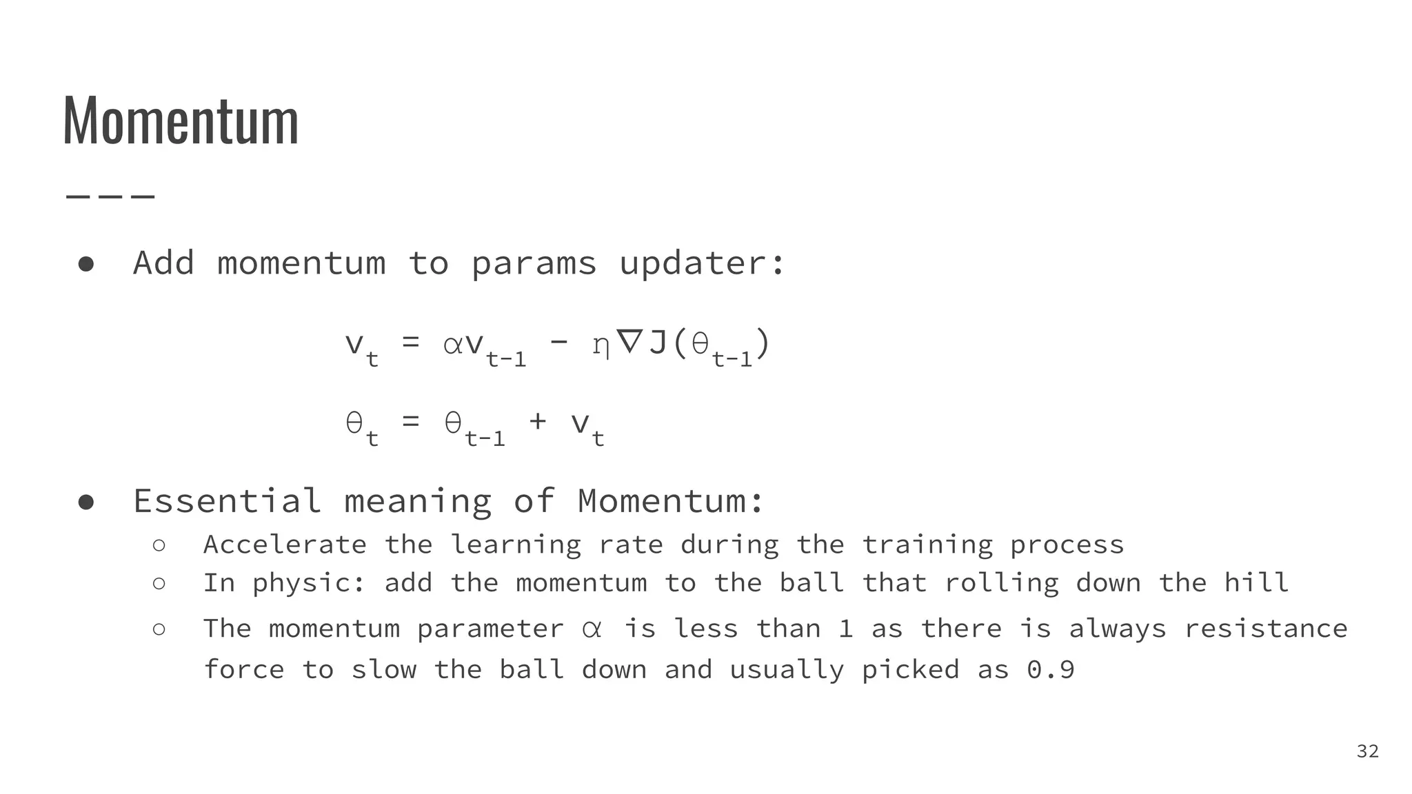
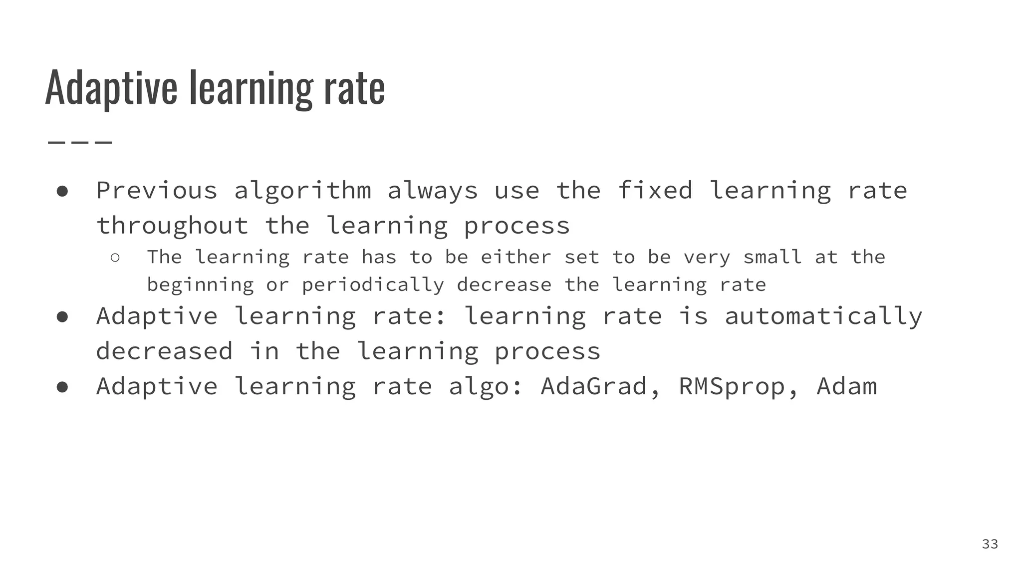
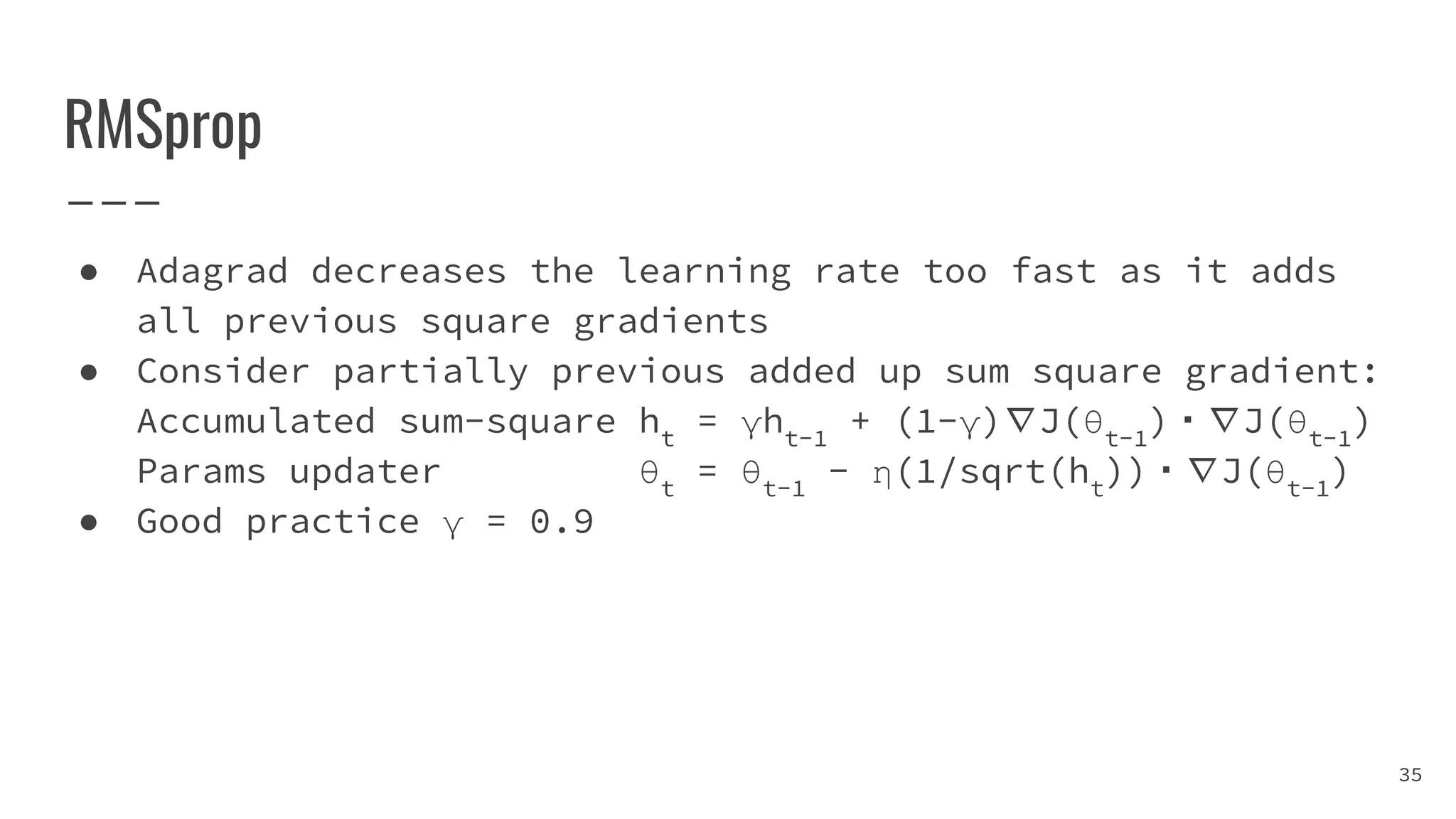
Overview of various practical algorithms like Momentum, AdaGrad, RMSprop, and Adam with their functionalities.
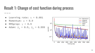
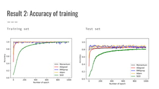
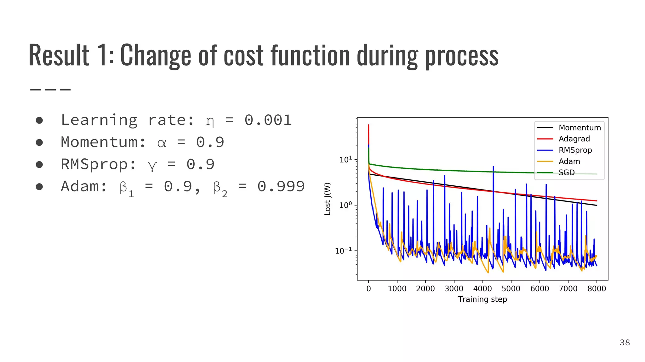
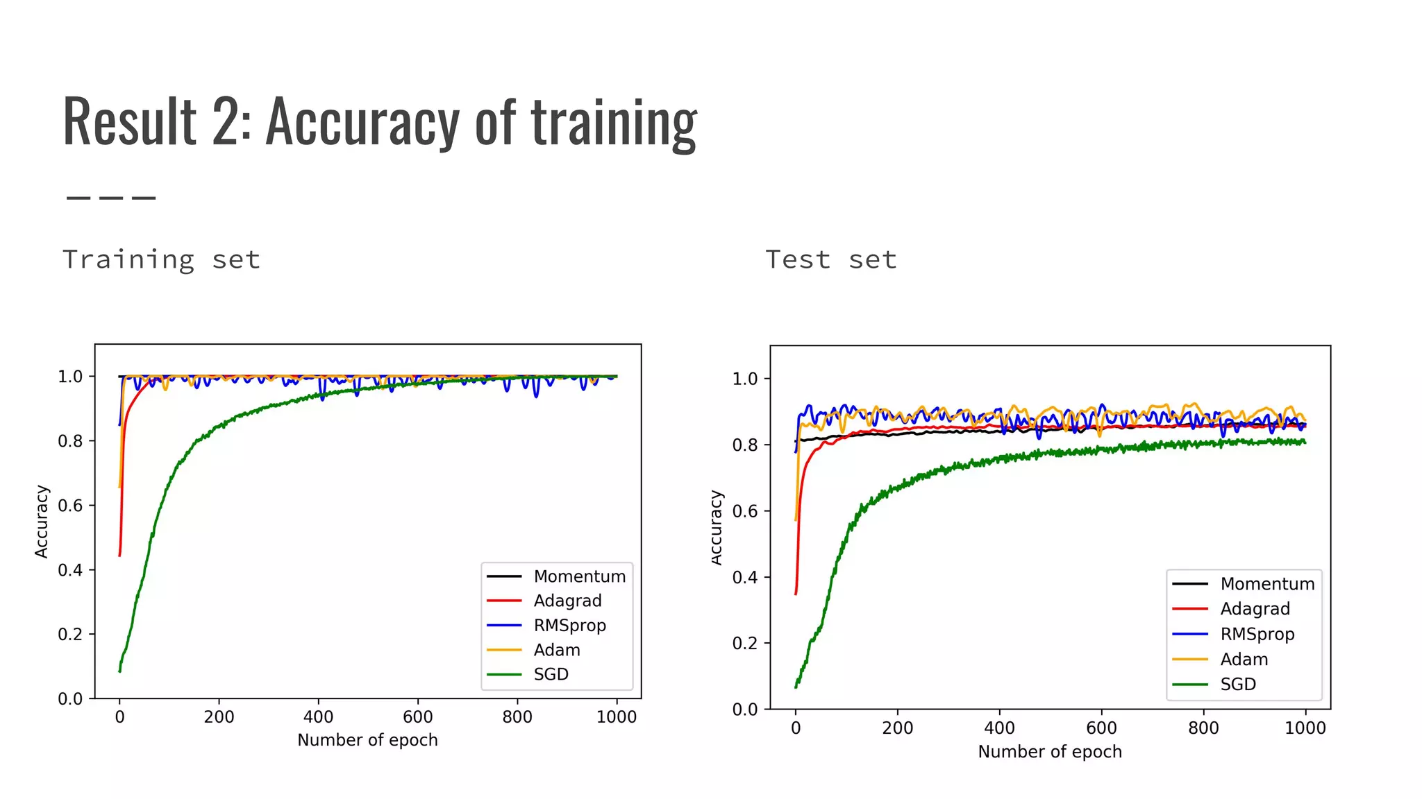
Results comparing different optimization algorithms using a neural network model on MNIST data set.
References for the content presented and a definition of machine learning.
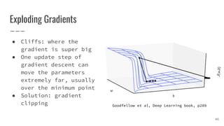
Explains issues like exploding and vanishing gradients in neural networks with proposed solutions.