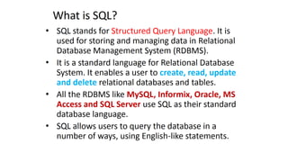
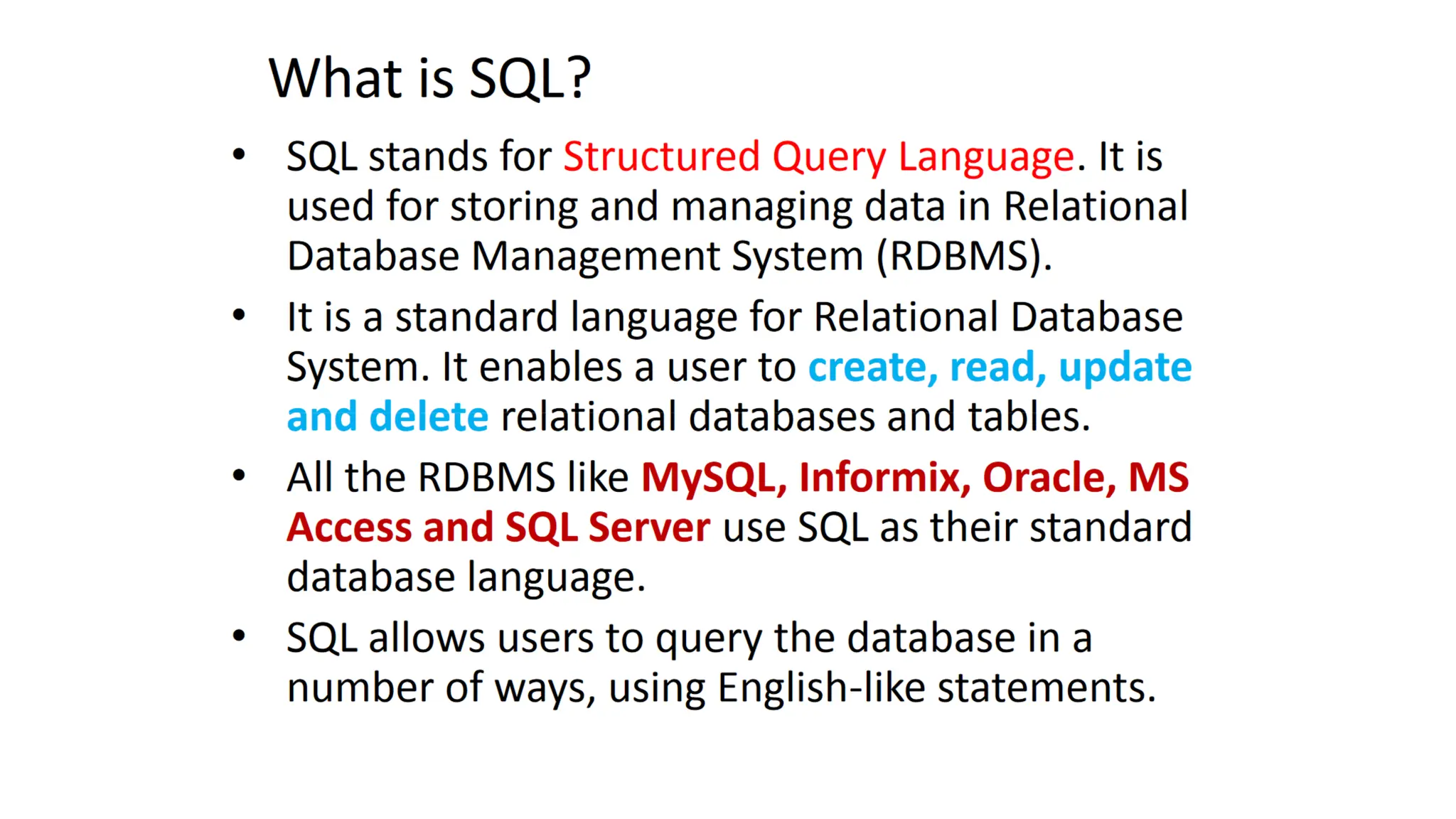
What are theSQL?
SQL follows the following rules:
• Structure query language is not case sensitive. Generally, keywords
of SQL are written in uppercase.
• Statements of SQL are dependent on text lines. We can use a
single SQL statement on one or multiple text line.
• Using the SQL statements, you can perform most of the actions in
a database.
• SQL depends on tuple relational calculus and relational algebra.
4.
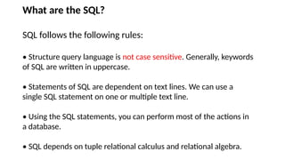
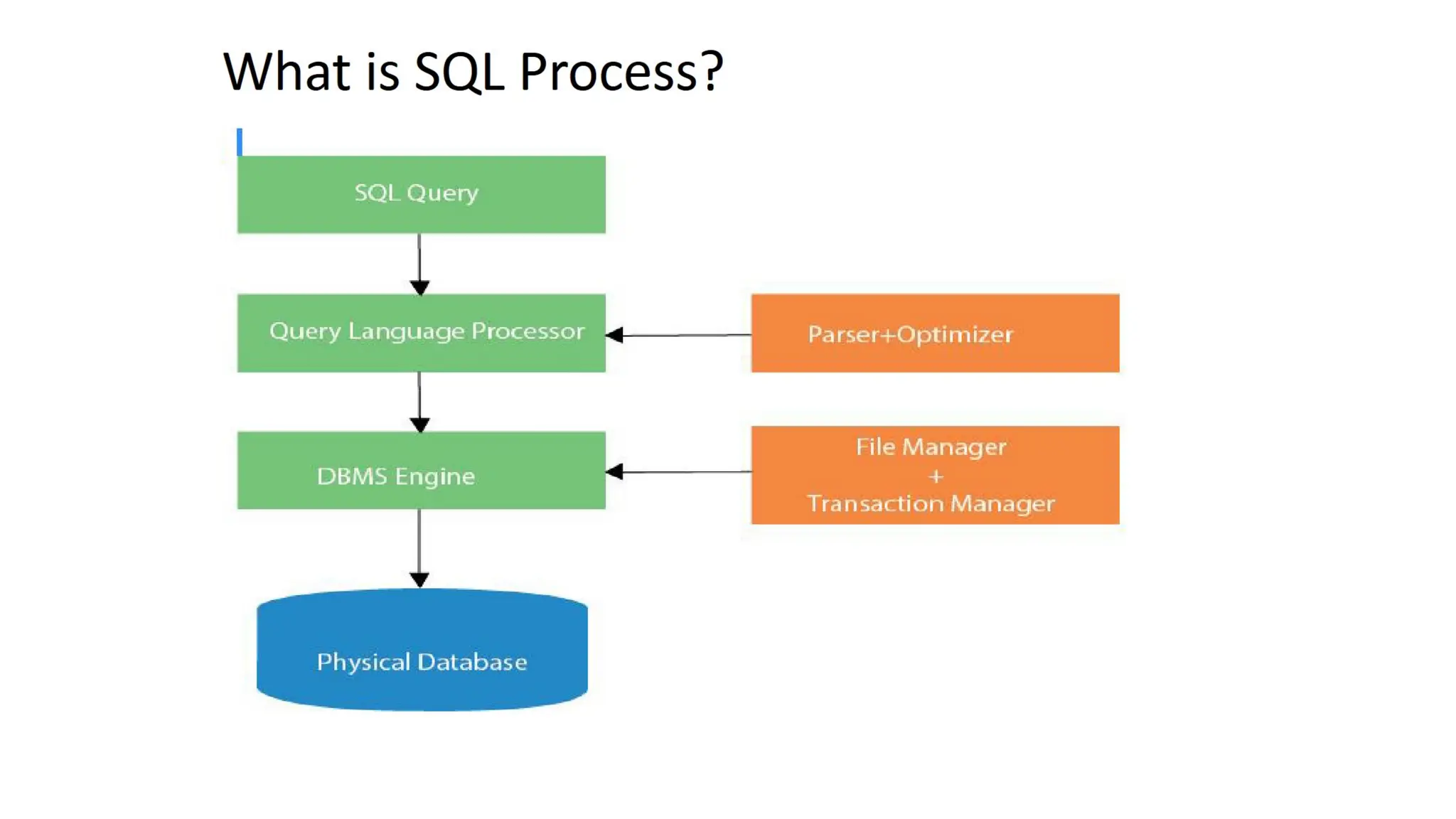
What is SQLProcess?
• When an SQL command is executing for any RDBMS, then
the system figure out the best way to carry out the request
and the SQL engine determines that how to interpret the
task.
• In the process, various components are included. These
components can be optimization Engine, Query engine,
Query dispatcher, classic, etc.
6.
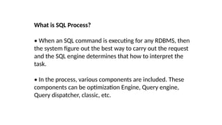
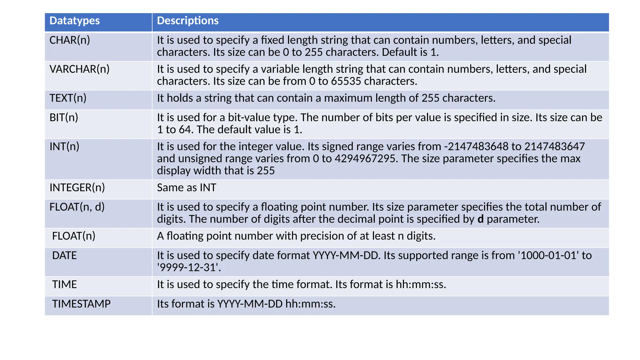
Datatypes Descriptions
CHAR(n) Itis used to specify a fixed length string that can contain numbers, letters, and special
characters. Its size can be 0 to 255 characters. Default is 1.
VARCHAR(n) It is used to specify a variable length string that can contain numbers, letters, and special
characters. Its size can be from 0 to 65535 characters.
TEXT(n) It holds a string that can contain a maximum length of 255 characters.
BIT(n) It is used for a bit-value type. The number of bits per value is specified in size. Its size can be
1 to 64. The default value is 1.
INT(n) It is used for the integer value. Its signed range varies from -2147483648 to 2147483647
and unsigned range varies from 0 to 4294967295. The size parameter specifies the max
display width that is 255
INTEGER(n) Same as INT
FLOAT(n, d) It is used to specify a floating point number. Its size parameter specifies the total number of
digits. The number of digits after the decimal point is specified by d parameter.
FLOAT(n) A floating point number with precision of at least n digits.
DATE It is used to specify date format YYYY-MM-DD. Its supported range is from '1000-01-01' to
'9999-12-31'.
TIME It is used to specify the time format. Its format is hh:mm:ss.
TIMESTAMP Its format is YYYY-MM-DD hh:mm:ss.
8.
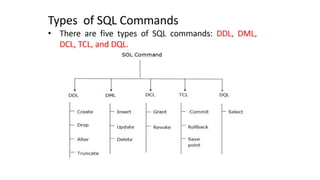
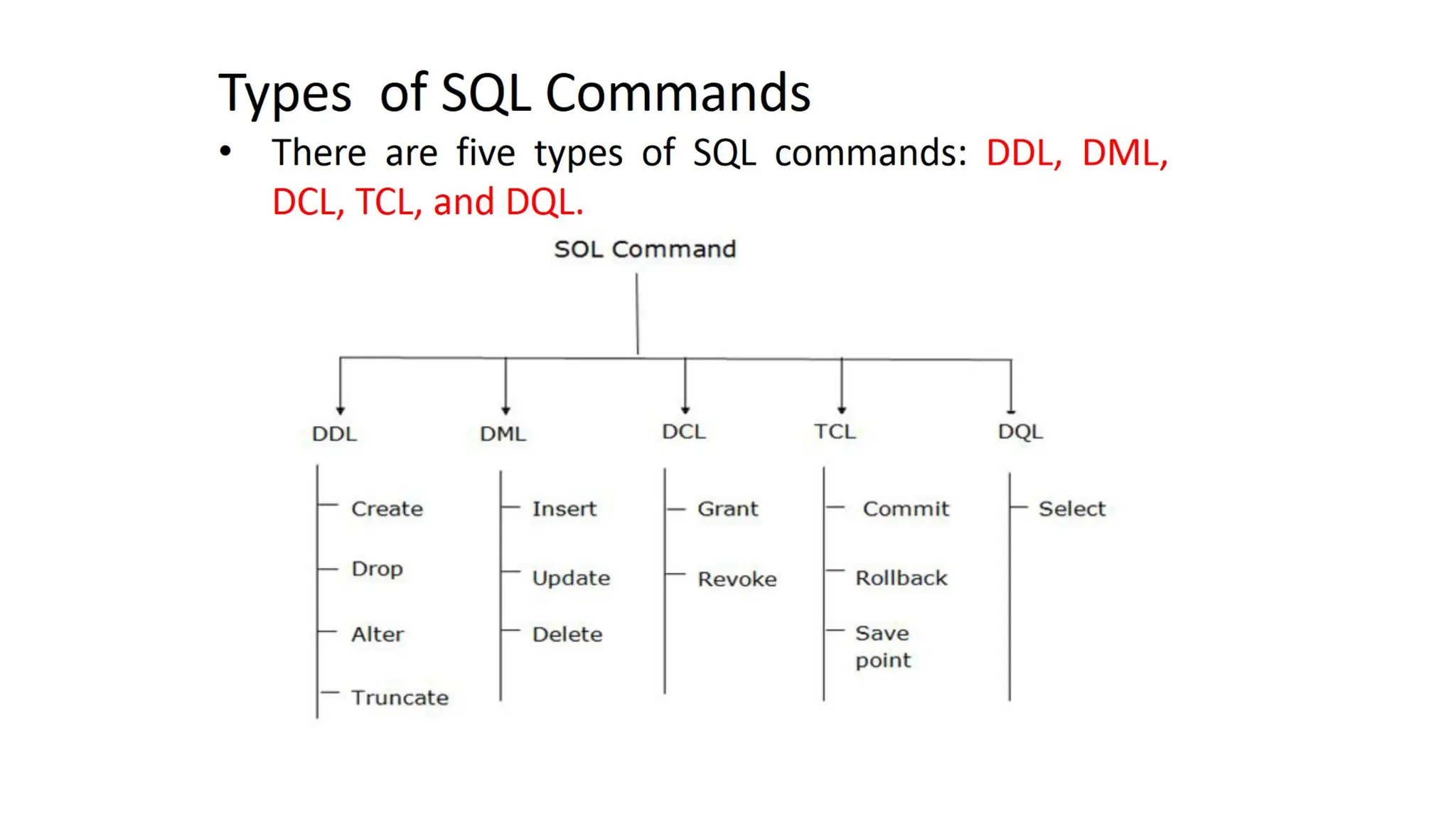
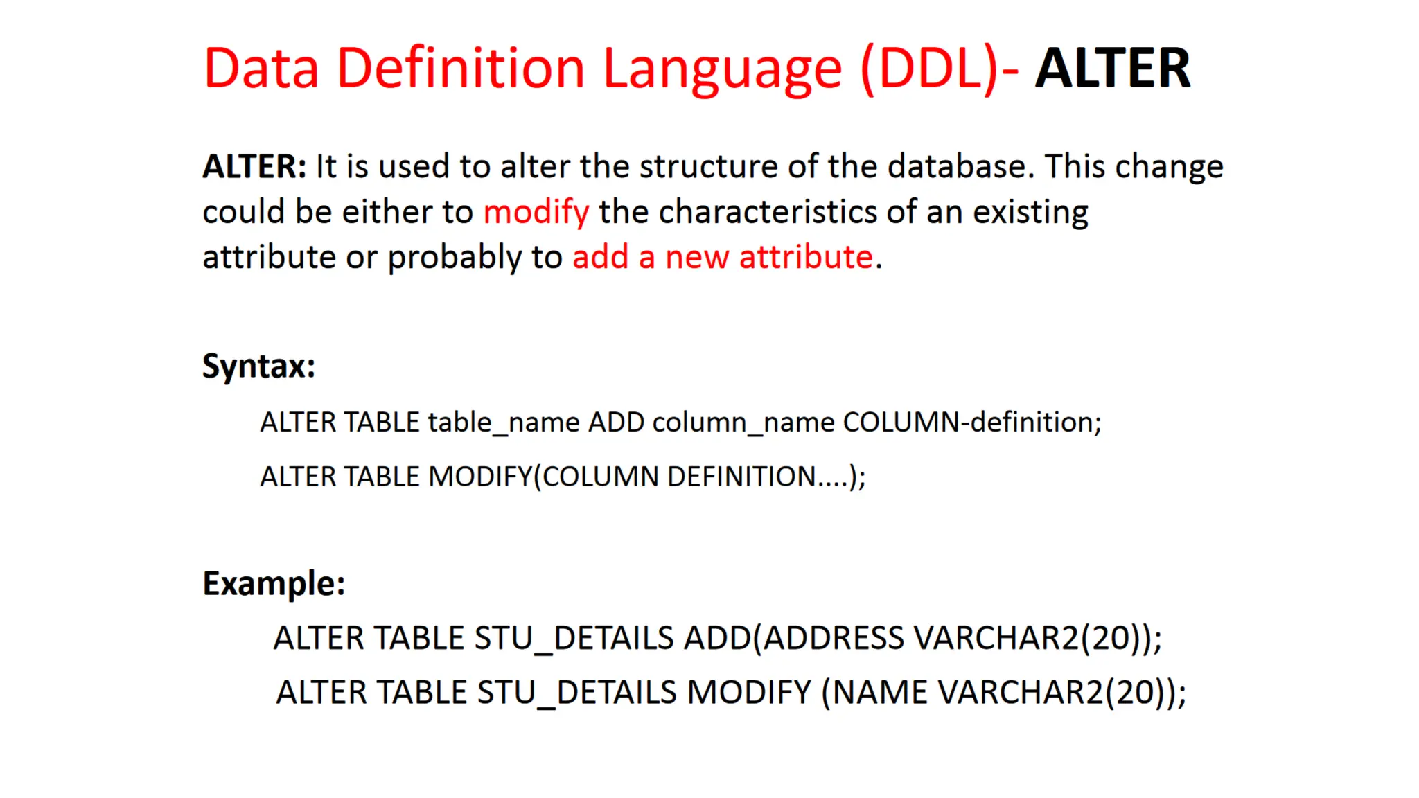
Data Definition Language(DDL)
• DDL changes the structure of the table like creating a
table, deleting a table, altering a table, etc.
• All the command of DDL are auto-committed that means
it permanently save all the changes in the database.
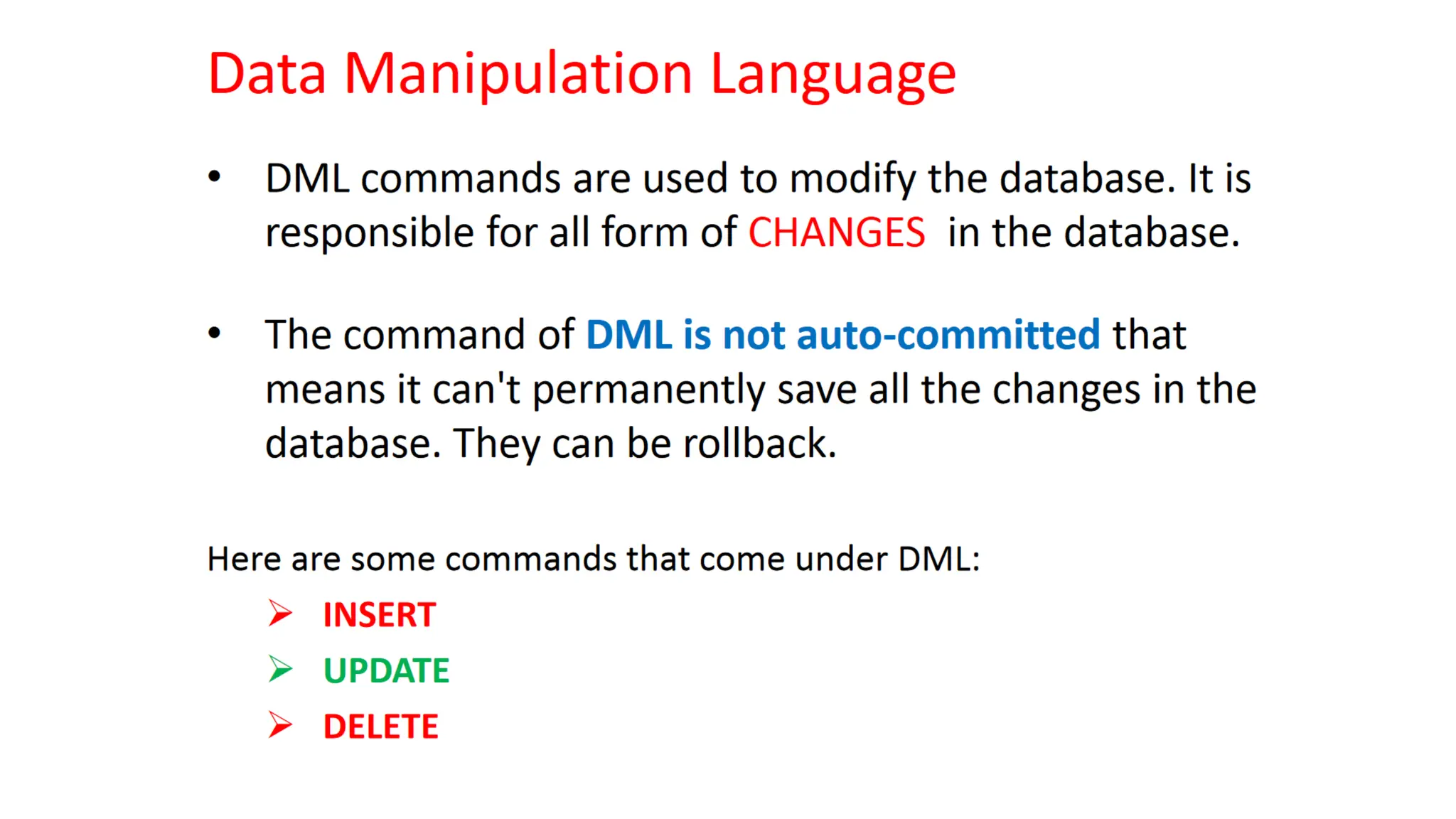
• Here are some commands that come under DDL:
CREATE
ALTER
DROP
9.
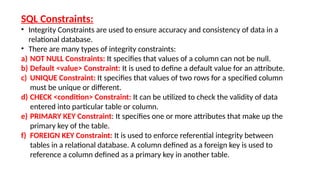
Data Definition Language(DDL)- CREATE
CREATE It is used to create a new table in the database.
Syntax:
create table r (A1 D1, A2 D2, ..., An Dn,
(integrity-constraint1),
...,
(integrity-constraintk))
r is the name of the relation
each Ai is an attribute name in the schema of relation r
Di is the data type of values in the domain of attribute Ai
Example:
create table instructor (
ID char(5),
name varchar(20),
dept_name varchar(20),
salary numeric(8,2))
10.
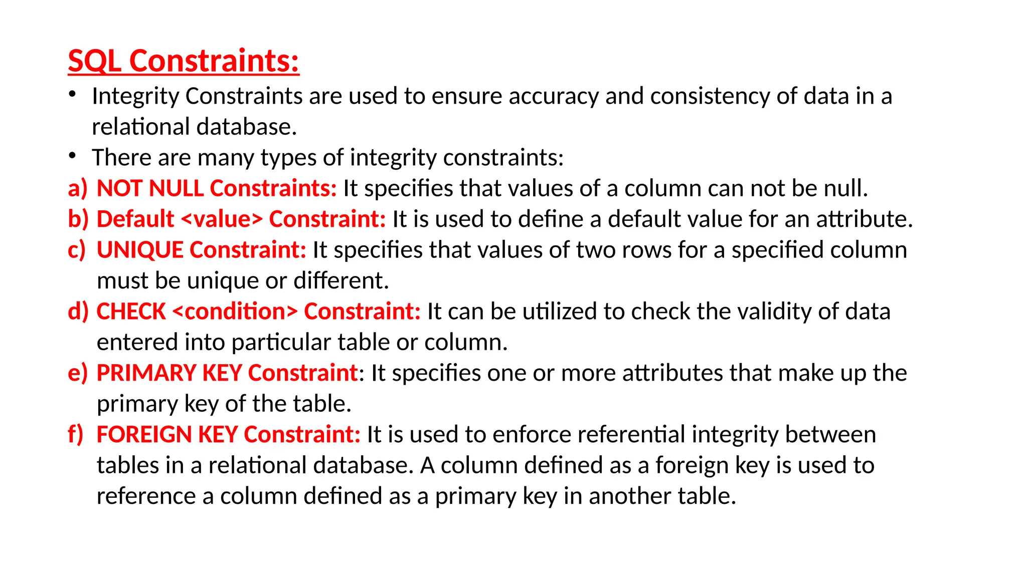
SQL Constraints:
• IntegrityConstraints are used to ensure accuracy and consistency of data in a
relational database.
• There are many types of integrity constraints:
a) NOT NULL Constraints: It specifies that values of a column can not be null.
b) Default <value> Constraint: It is used to define a default value for an attribute.
c) UNIQUE Constraint: It specifies that values of two rows for a specified column
must be unique or different.
d) CHECK <condition> Constraint: It can be utilized to check the validity of data
entered into particular table or column.
e) PRIMARY KEY Constraint: It specifies one or more attributes that make up the
primary key of the table.
f) FOREIGN KEY Constraint: It is used to enforce referential integrity between
tables in a relational database. A column defined as a foreign key is used to
reference a column defined as a primary key in another table.
11.
CREATE TABLE [CUSTOMER]
(
CustomerIdint IDENTITY(1,1) PRIMARY KEY,
CustomerNumber int NOT NULL UNIQUE,
LastName varchar(50) NOT NULL,
FirstName varchar(50) NOT NULL,
AreaCode int NULL,
Address varchar(50) NULL,
Phone varchar(50) NULL,
)
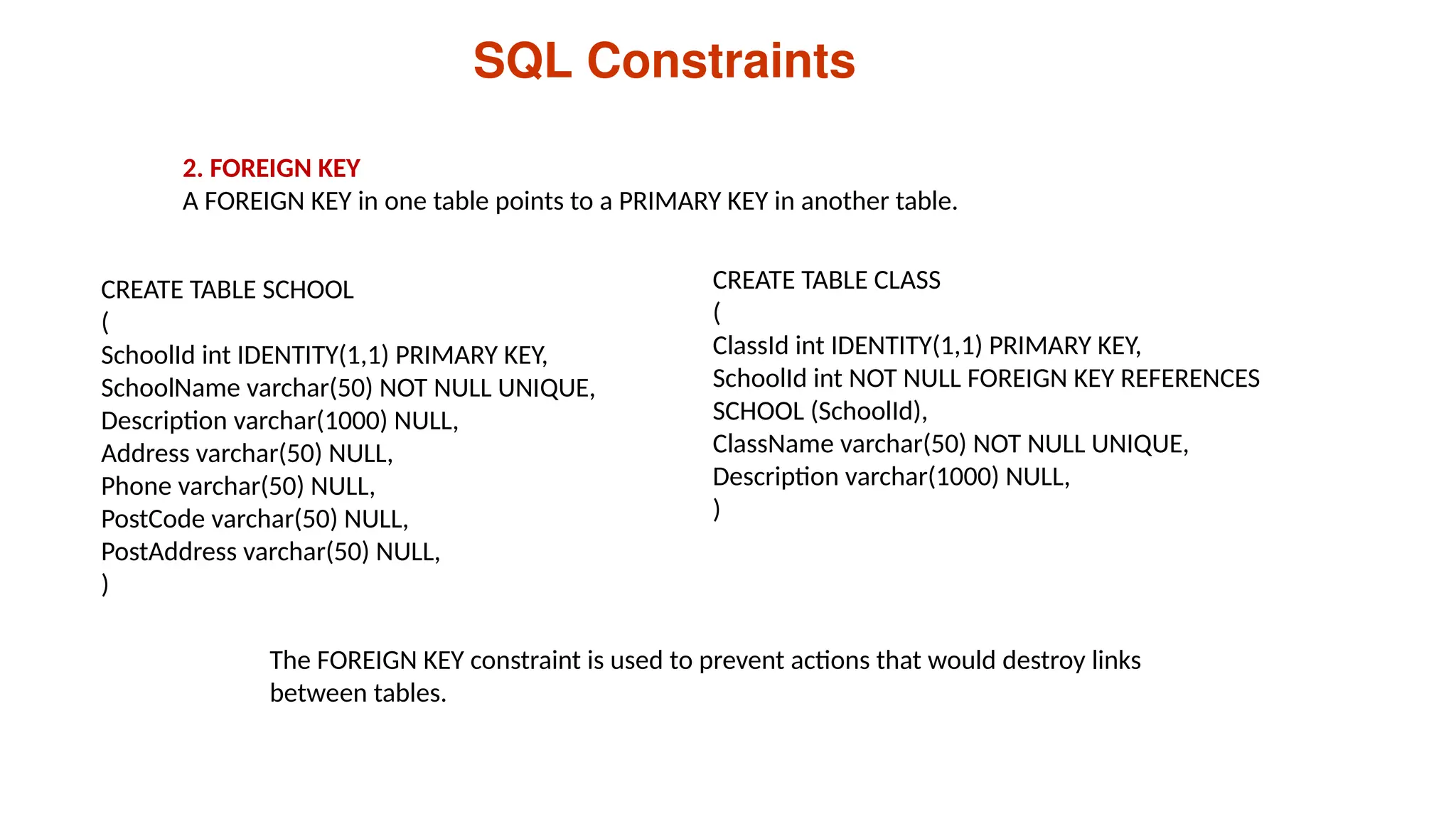
SQL Constraints
1. PRIMARY KEY
The PRIMARY KEY constraint uniquely identifies each record in a database table.
Each table should have a primary key, and each table can have only ONE primary key.
Here, IDENTITY(1,1) means the first value will be 1 and then it will increment by 1.
12.
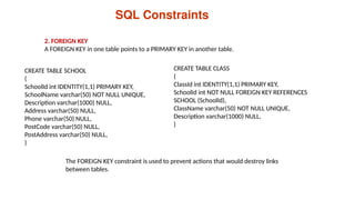
CREATE TABLE SCHOOL
(
SchoolIdint IDENTITY(1,1) PRIMARY KEY,
SchoolName varchar(50) NOT NULL UNIQUE,
Description varchar(1000) NULL,
Address varchar(50) NULL,
Phone varchar(50) NULL,
PostCode varchar(50) NULL,
PostAddress varchar(50) NULL,
)
SQL Constraints
2. FOREIGN KEY
A FOREIGN KEY in one table points to a PRIMARY KEY in another table.
The FOREIGN KEY constraint is used to prevent actions that would destroy links
between tables.
CREATE TABLE CLASS
(
ClassId int IDENTITY(1,1) PRIMARY KEY,
SchoolId int NOT NULL FOREIGN KEY REFERENCES
SCHOOL (SchoolId),
ClassName varchar(50) NOT NULL UNIQUE,
Description varchar(1000) NULL,
)
13.
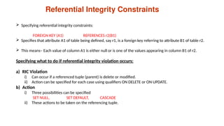
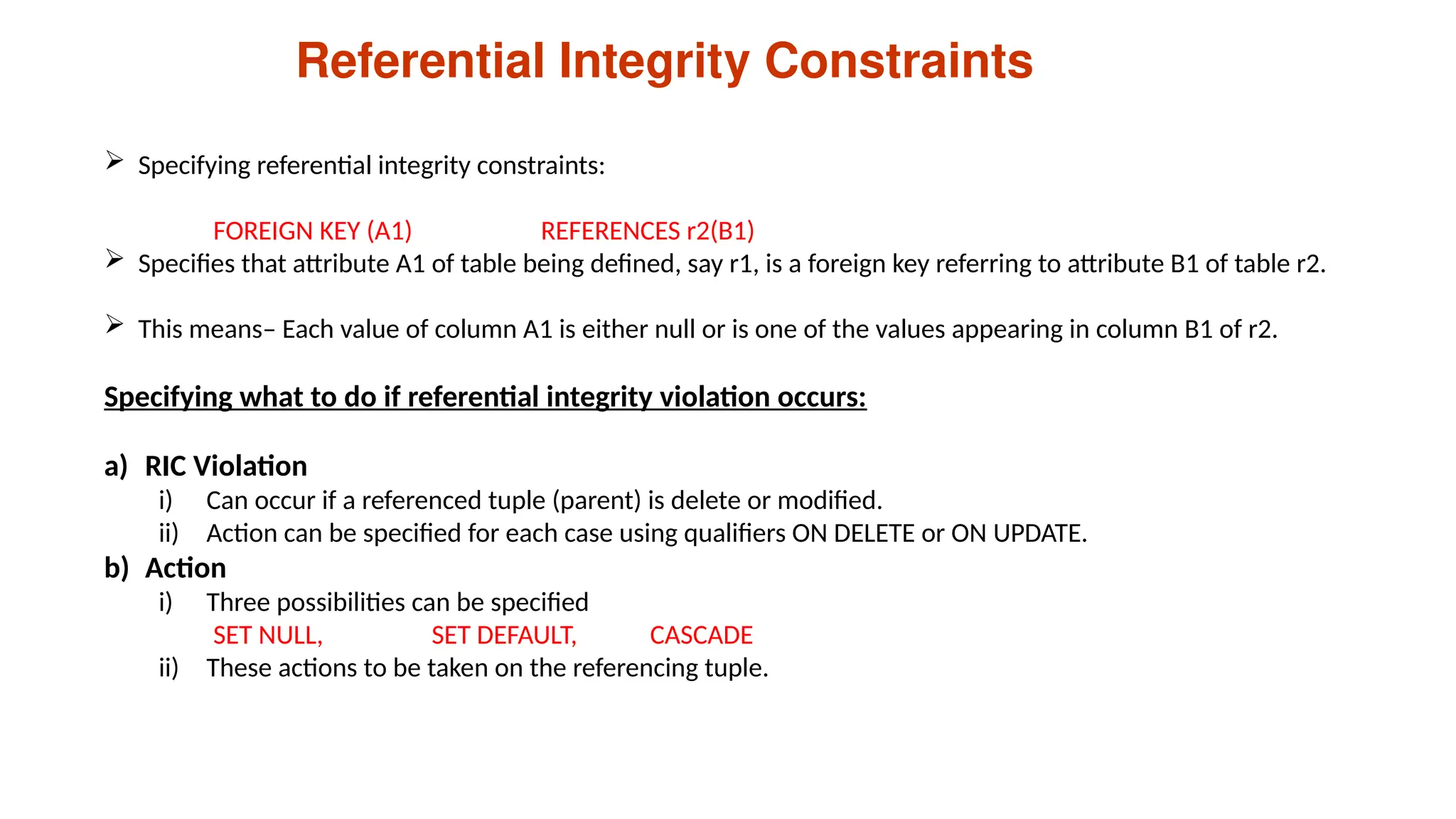
Referential Integrity Constraints
Specifying referential integrity constraints:
FOREIGN KEY (A1) REFERENCES r2(B1)
Specifies that attribute A1 of table being defined, say r1, is a foreign key referring to attribute B1 of table r2.
This means– Each value of column A1 is either null or is one of the values appearing in column B1 of r2.
Specifying what to do if referential integrity violation occurs:
a) RIC Violation
i) Can occur if a referenced tuple (parent) is delete or modified.
ii) Action can be specified for each case using qualifiers ON DELETE or ON UPDATE.
b) Action
i) Three possibilities can be specified
SET NULL, SET DEFAULT, CASCADE
ii) These actions to be taken on the referencing tuple.
14.
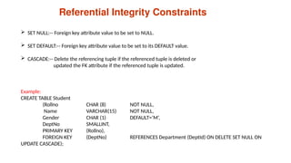
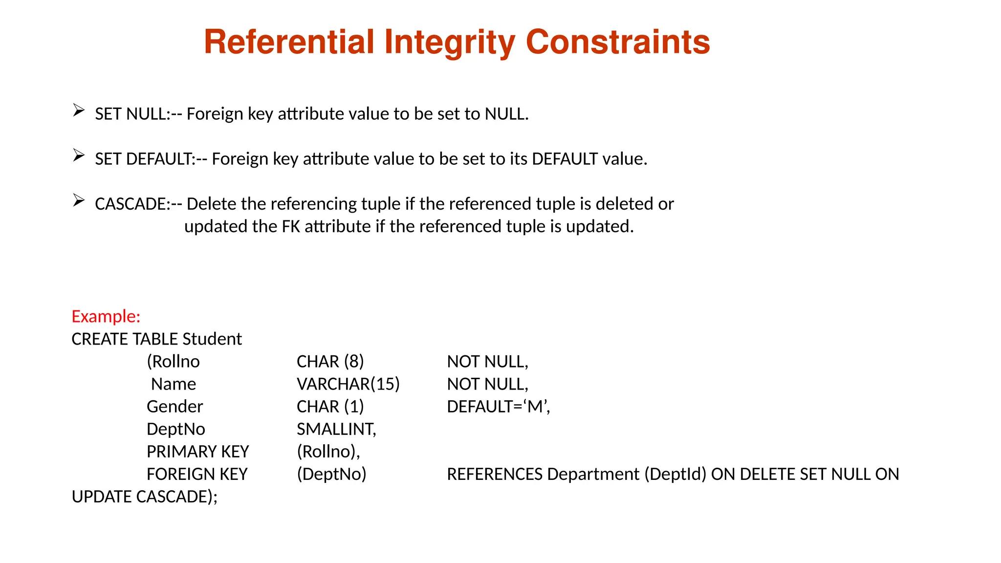
Referential Integrity Constraints
SET NULL:-- Foreign key attribute value to be set to NULL.
SET DEFAULT:-- Foreign key attribute value to be set to its DEFAULT value.
CASCADE:-- Delete the referencing tuple if the referenced tuple is deleted or
updated the FK attribute if the referenced tuple is updated.
Example:
CREATE TABLE Student
(Rollno CHAR (8) NOT NULL,
Name VARCHAR(15) NOT NULL,
Gender CHAR (1) DEFAULT=‘M’,
DeptNo SMALLINT,
PRIMARY KEY (Rollno),
FOREIGN KEY (DeptNo) REFERENCES Department (DeptId) ON DELETE SET NULL ON
UPDATE CASCADE);
15.
SQL Constraints
3. NOTNULL / Required Columns
The NOT NULL constraint enforces a column to NOT accept NULL values.
The NOT NULL constraint enforces a field to always contain a value.
This means that you cannot insert a new record, or update a record without adding a value to
this field
CREATE TABLE [CUSTOMER]
(
CustomerId int IDENTITY(1,1) PRIMARY KEY,
CustomerNumber int NOT NULL UNIQUE,
LastName varchar(50) NOT NULL,
FirstName varchar(50) NOT NULL,
AreaCode int NULL,
Address varchar(50) NULL,
Phone varchar(50) NULL,
)
Note! A primary key column cannot contain NULL values.
16.
SQL Constraints
4. UNIQUE
The UNIQUE constraint uniquely identifies each record in a database table.
The UNIQUE and PRIMARY KEY constraints both provide a guarantee for uniqueness for a column
or set of columns.
A PRIMARY KEY constraint automatically has a UNIQUE constraint defined on it.
Note! You can have many UNIQUE constraints per table, but only one PRIMARY KEY constraint per
table.
CREATE TABLE [CUSTOMER]
(
CustomerId int IDENTITY(1,1) PRIMARY KEY,
CustomerNumber int NOT NULL UNIQUE,
LastName varchar(50) NOT NULL,
FirstName varchar(50) NOT NULL,
AreaCode int NULL,
Address varchar(50) NULL,
Phone varchar(50) NULL,
)
17.
5. CHECK
TheCHECK constraint is used to limit the value range that can be placed in a column.
SQL Constraints
CREATE TABLE [CUSTOMER]
(
CustomerId int IDENTITY(1,1) PRIMARY KEY,
CustomerNumber int NOT NULL UNIQUE CHECK(CustomerNumber>0),
LastName varchar(50) NOT NULL,
FirstName varchar(50) NOT NULL,
AreaCode int NULL,
Address varchar(50) NULL,
Phone varchar(50) NULL,
)
18.
6. DEFAULT
TheDEFAULT constraint is used to insert a default value into a column.
The default value will be added to all new records, if no other value is specified..
SQL Constraints
CREATE TABLE [CUSTOMER]
(
CustomerId int IDENTITY(1,1) PRIMARY KEY,
CustomerNumber int NOT NULL UNIQUE,
LastName varchar(50) NOT NULL,
FirstName varchar(50) NOT NULL,
Country varchar(20) DEFAULT 'Norway',
AreaCode int NULL,
Address varchar(50) NULL,
Phone varchar(50) NULL,
)
19.
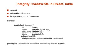
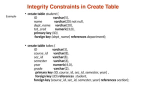
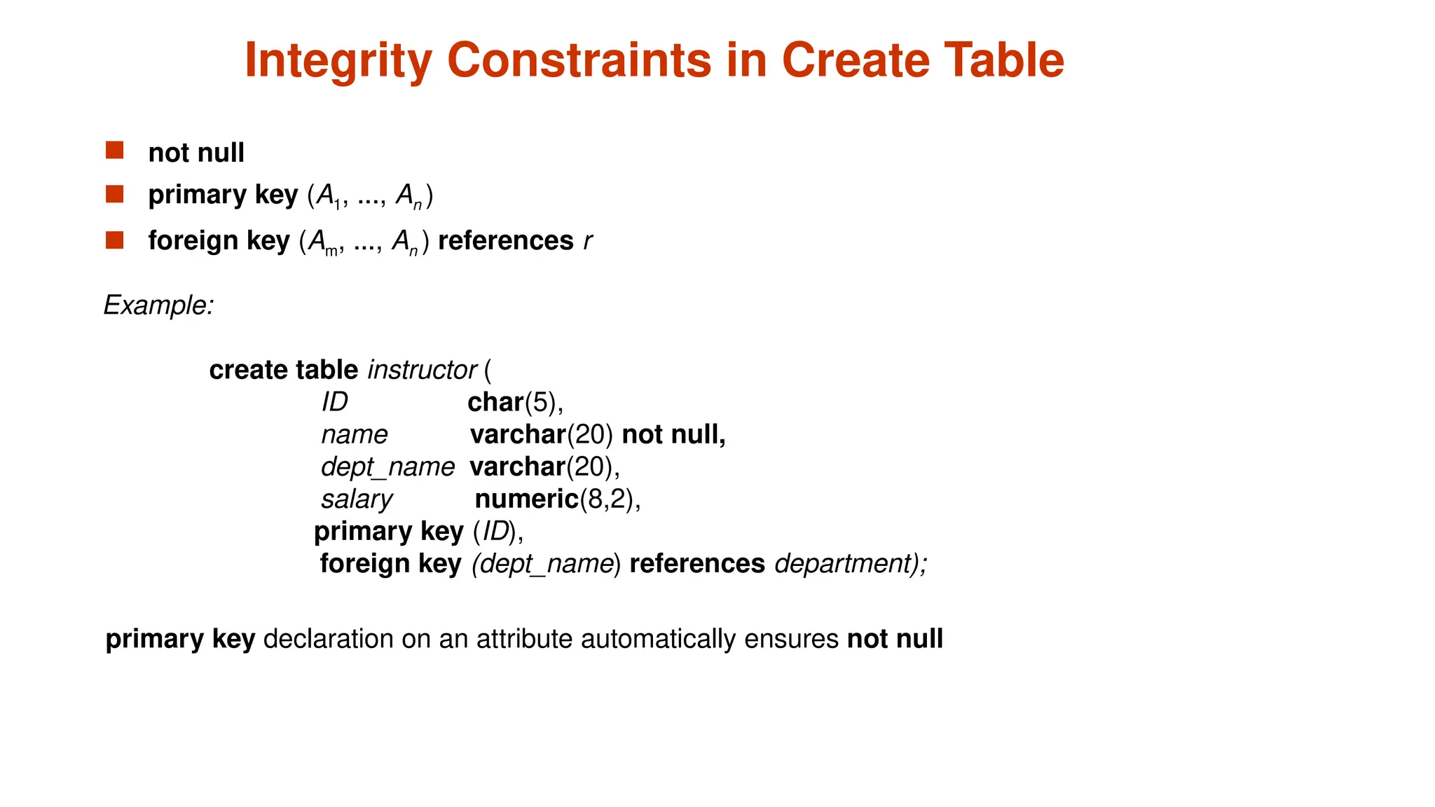
Integrity Constraints inCreate Table
not null
primary key (A1, ..., An )
foreign key (Am, ..., An ) references r
Example:
create table instructor (
ID char(5),
name varchar(20) not null,
dept_name varchar(20),
salary numeric(8,2),
primary key (ID),
foreign key (dept_name) references department);
primary key declaration on an attribute automatically ensures not null
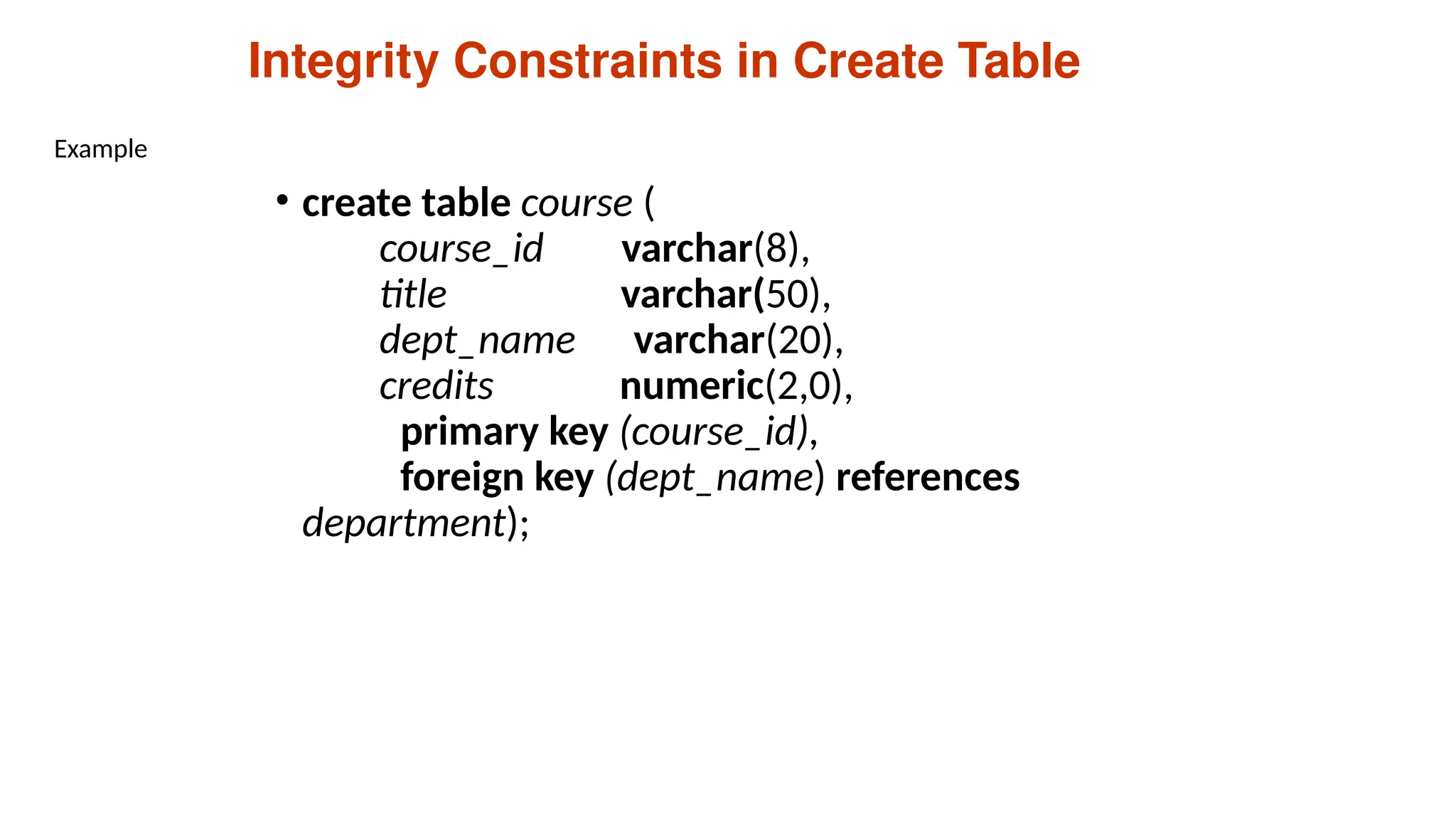
• create tablecourse (
course_id varchar(8),
title varchar(50),
dept_name varchar(20),
credits numeric(2,0),
primary key (course_id),
foreign key (dept_name) references
department);
Integrity Constraints in Create Table
Example
22.
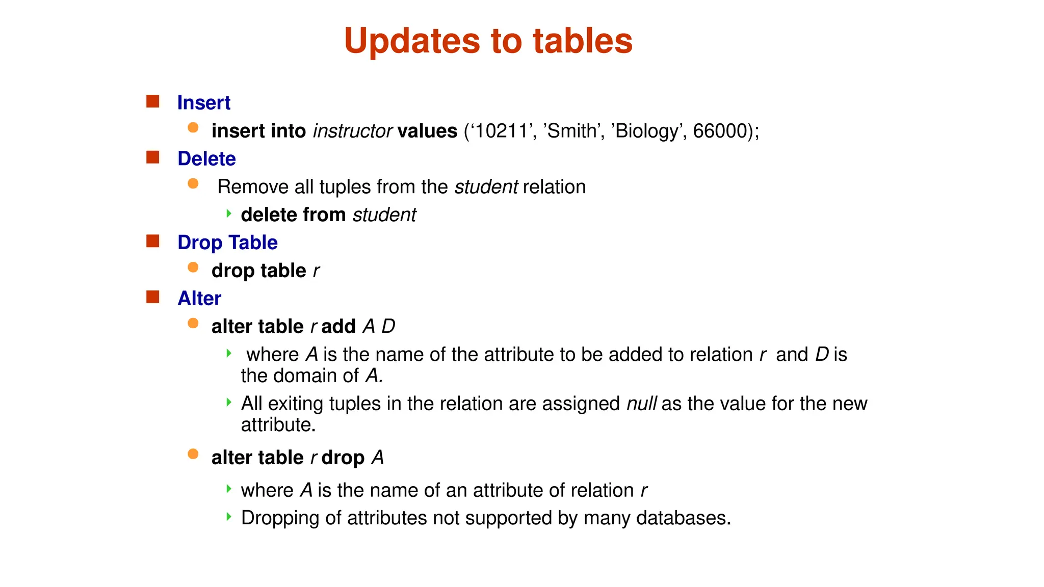
Updates to tables
Insert
insert into instructor values (‘10211’, ’Smith’, ’Biology’, 66000);
Delete
Remove all tuples from the student relation
delete from student
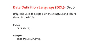
Drop Table
drop table r
Alter
alter table r add A D
where A is the name of the attribute to be added to relation r and D is
the domain of A.
All exiting tuples in the relation are assigned null as the value for the new
attribute.
alter table r drop A
where A is the name of an attribute of relation r
Dropping of attributes not supported by many databases.
23.
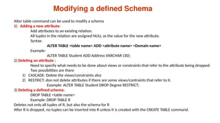
Modifying a definedSchema
Alter table command can be used to modify a schema
1) Adding a new attribute:
Add attributes to an existing relation.
All tuples in the relation are assigned NULL as the value for the new attribute.
Syntax:
ALTER TABLE <table name> ADD <attribute name> <Domain name>
Example:
ALTER TABLE Student ADD Address VARCHAR (30);
2) Deleting an attribute :
Need to specify what needs to be done about views or constraints that refer to the attribute being dropped.
Two possibilities are there
1) CASCADE: Delete the views/constraints also
2) RESTRICT: don not delete attributes if there are some views/contraints that refer to it.
Example: ALTER TABLE Student DROP Degree RESTRICT;
3) Deleting a defined schema:
DROP TABLE <table name>
Example: DROP TABLE R
Deletes not only all tuples of R, but also the schema for R
After R is dropped, no tuples can be inserted into R unless it is created with the CREATE TABLE command.
28.
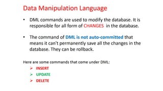
Data Manipulation Language(DML)
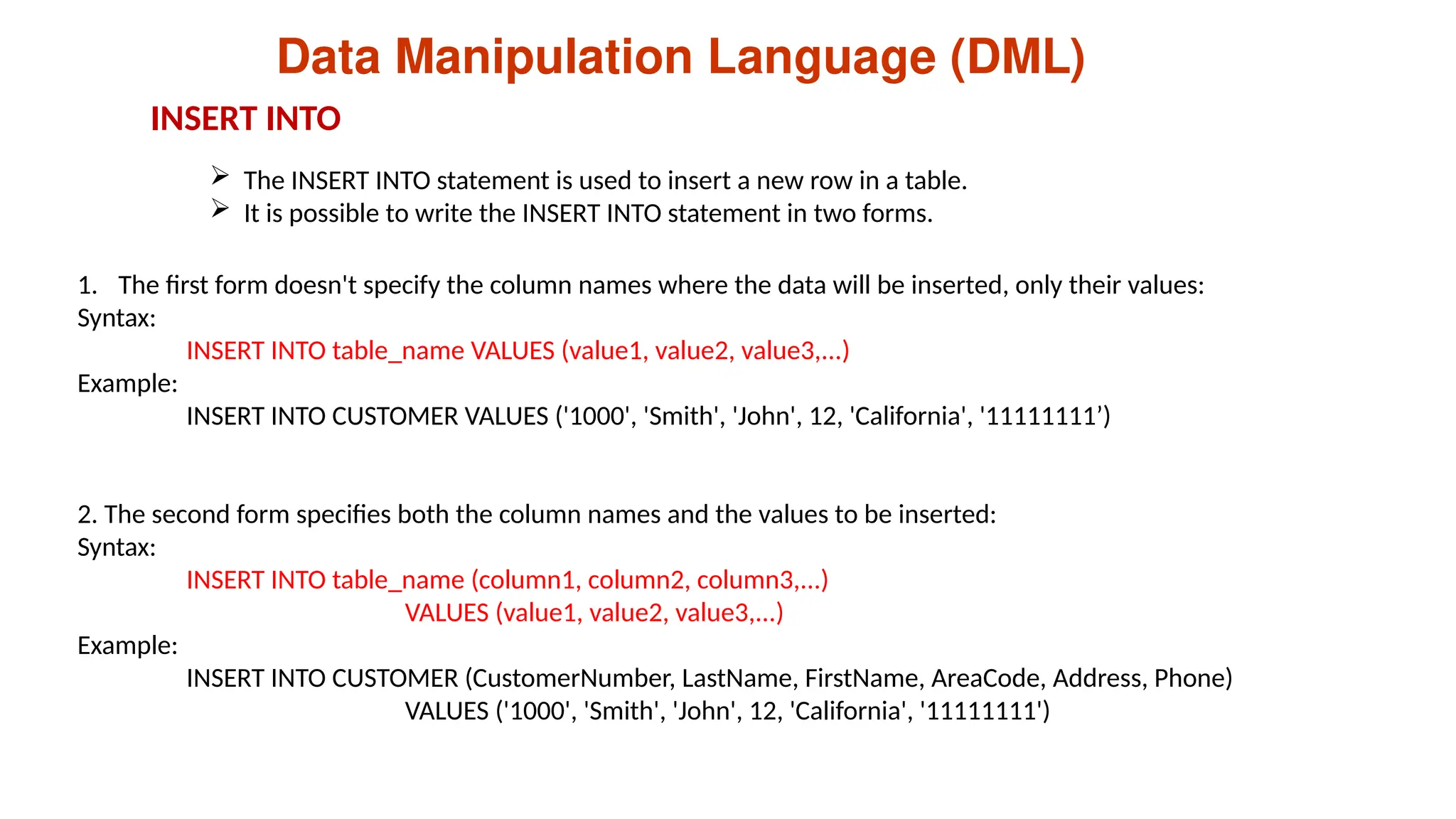
The INSERT INTO statement is used to insert a new row in a table.
It is possible to write the INSERT INTO statement in two forms.
1. The first form doesn't specify the column names where the data will be inserted, only their values:
Syntax:
INSERT INTO table_name VALUES (value1, value2, value3,...)
Example:
INSERT INTO CUSTOMER VALUES ('1000', 'Smith', 'John', 12, 'California', '11111111’)
2. The second form specifies both the column names and the values to be inserted:
Syntax:
INSERT INTO table_name (column1, column2, column3,...)
VALUES (value1, value2, value3,...)
Example:
INSERT INTO CUSTOMER (CustomerNumber, LastName, FirstName, AreaCode, Address, Phone)
VALUES ('1000', 'Smith', 'John', 12, 'California', '11111111')
INSERT INTO
29.
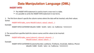
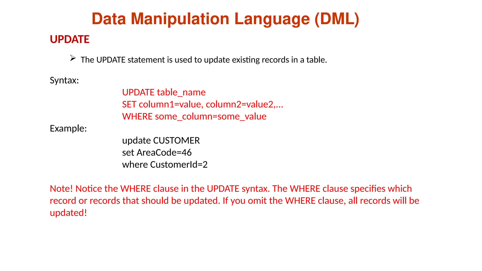
Data Manipulation Language(DML)
The UPDATE statement is used to update existing records in a table.
UPDATE
Syntax:
UPDATE table_name
SET column1=value, column2=value2,...
WHERE some_column=some_value
Example:
update CUSTOMER
set AreaCode=46
where CustomerId=2
Note! Notice the WHERE clause in the UPDATE syntax. The WHERE clause specifies which
record or records that should be updated. If you omit the WHERE clause, all records will be
updated!
31.
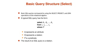
Basic Query Structure(Select)
Basic SQL queries correspond to using the SELECT, PROJECT, and JOIN
operations of the relational algebra
A typical SQL query has the form:
select A1, A2, ..., An
from r1, r2, ..., rm
where P
Ai represents an attribute
Ri represents a relation
P is a predicate.
The result of an SQL query is a relation.
32.
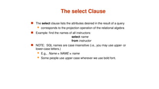
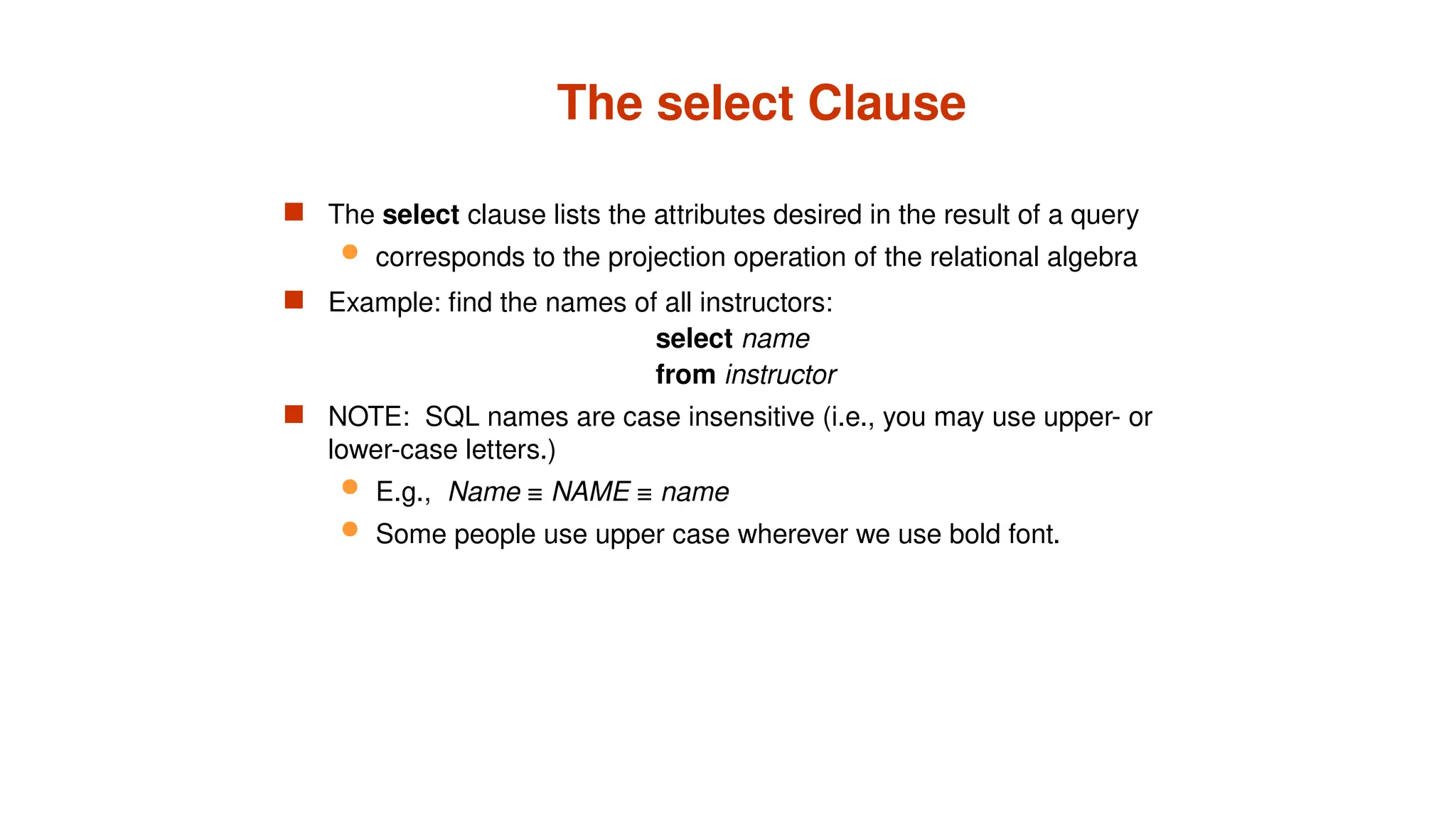
The select Clause
The select clause lists the attributes desired in the result of a query
corresponds to the projection operation of the relational algebra
Example: find the names of all instructors:
select name
from instructor
NOTE: SQL names are case insensitive (i.e., you may use upper- or
lower-case letters.)
E.g., Name ≡ NAME ≡ name
Some people use upper case wherever we use bold font.
33.
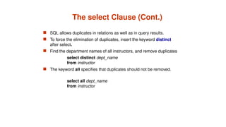
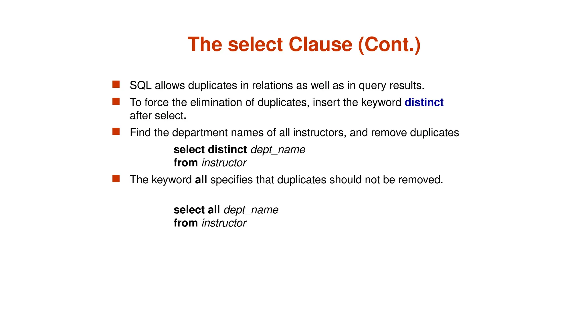
The select Clause(Cont.)
SQL allows duplicates in relations as well as in query results.
To force the elimination of duplicates, insert the keyword distinct
after select.
Find the department names of all instructors, and remove duplicates
select distinct dept_name
from instructor
The keyword all specifies that duplicates should not be removed.
select all dept_name
from instructor
34.
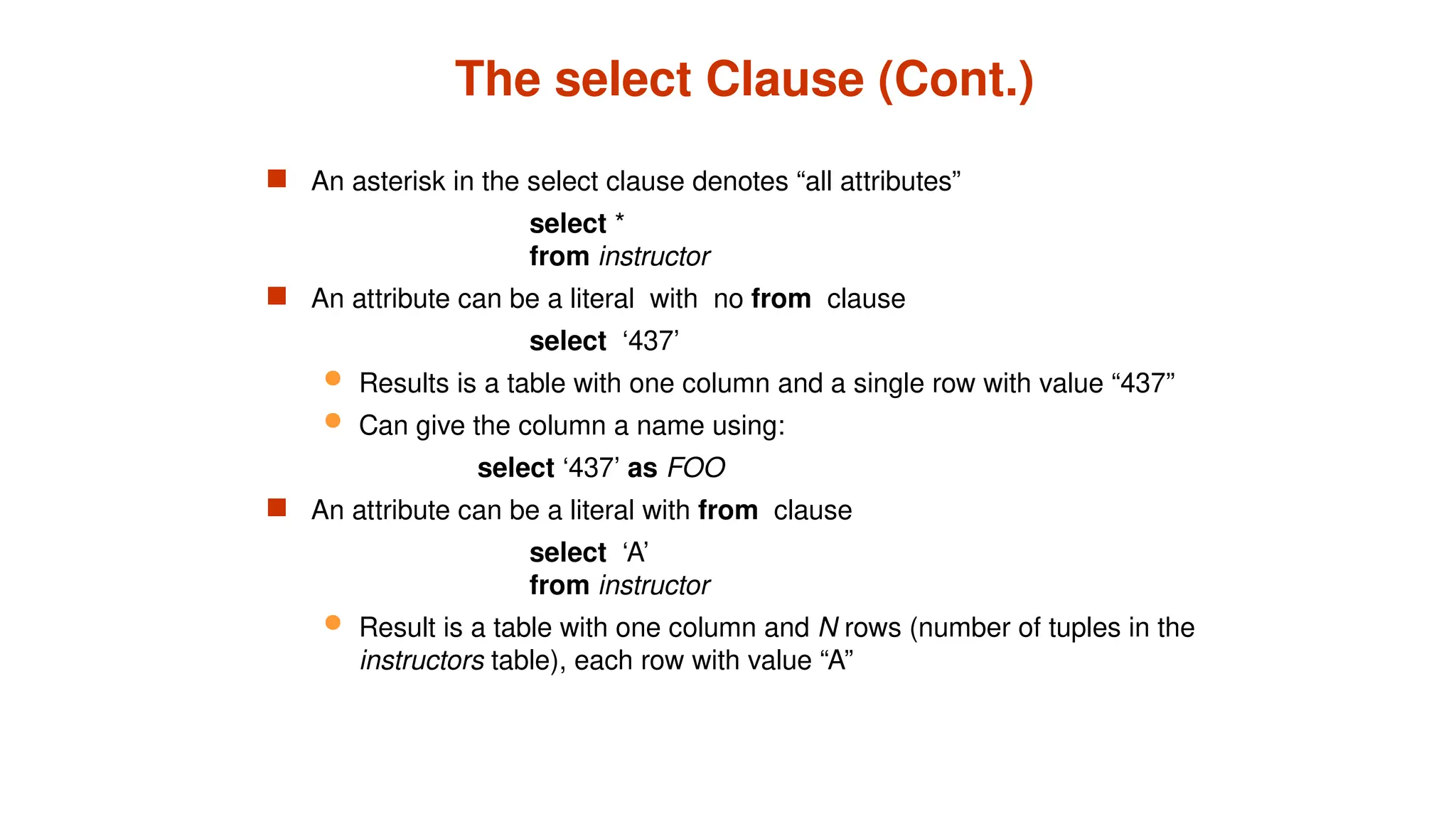
The select Clause(Cont.)
An asterisk in the select clause denotes “all attributes”
select *
from instructor
An attribute can be a literal with no from clause
select ‘437’
Results is a table with one column and a single row with value “437”
Can give the column a name using:
select ‘437’ as FOO
An attribute can be a literal with from clause
select ‘A’
from instructor
Result is a table with one column and N rows (number of tuples in the
instructors table), each row with value “A”
35.
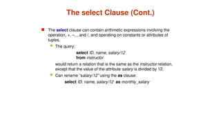
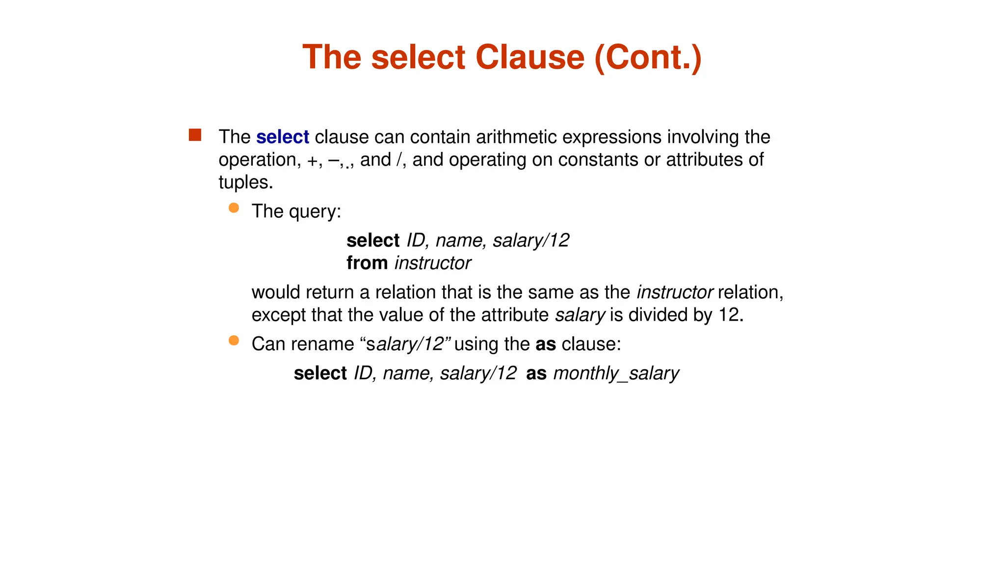
The select Clause(Cont.)
The select clause can contain arithmetic expressions involving the
operation, +, –, , and /, and operating on constants or attributes of
tuples.
The query:
select ID, name, salary/12
from instructor
would return a relation that is the same as the instructor relation,
except that the value of the attribute salary is divided by 12.
Can rename “salary/12” using the as clause:
select ID, name, salary/12 as monthly_salary
36.
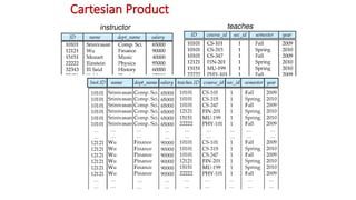
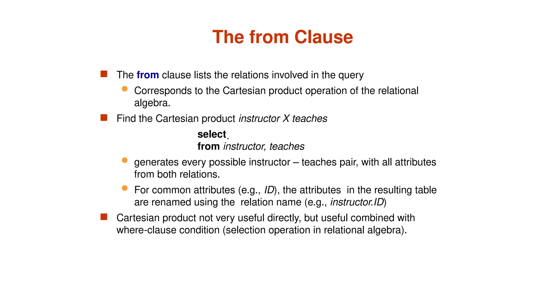
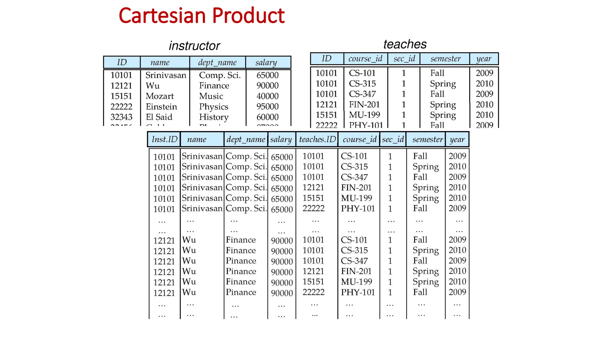
The from Clause
The from clause lists the relations involved in the query
Corresponds to the Cartesian product operation of the relational
algebra.
Find the Cartesian product instructor X teaches
select
from instructor, teaches
generates every possible instructor – teaches pair, with all attributes
from both relations.
For common attributes (e.g., ID), the attributes in the resulting table
are renamed using the relation name (e.g., instructor.ID)
Cartesian product not very useful directly, but useful combined with
where-clause condition (selection operation in relational algebra).
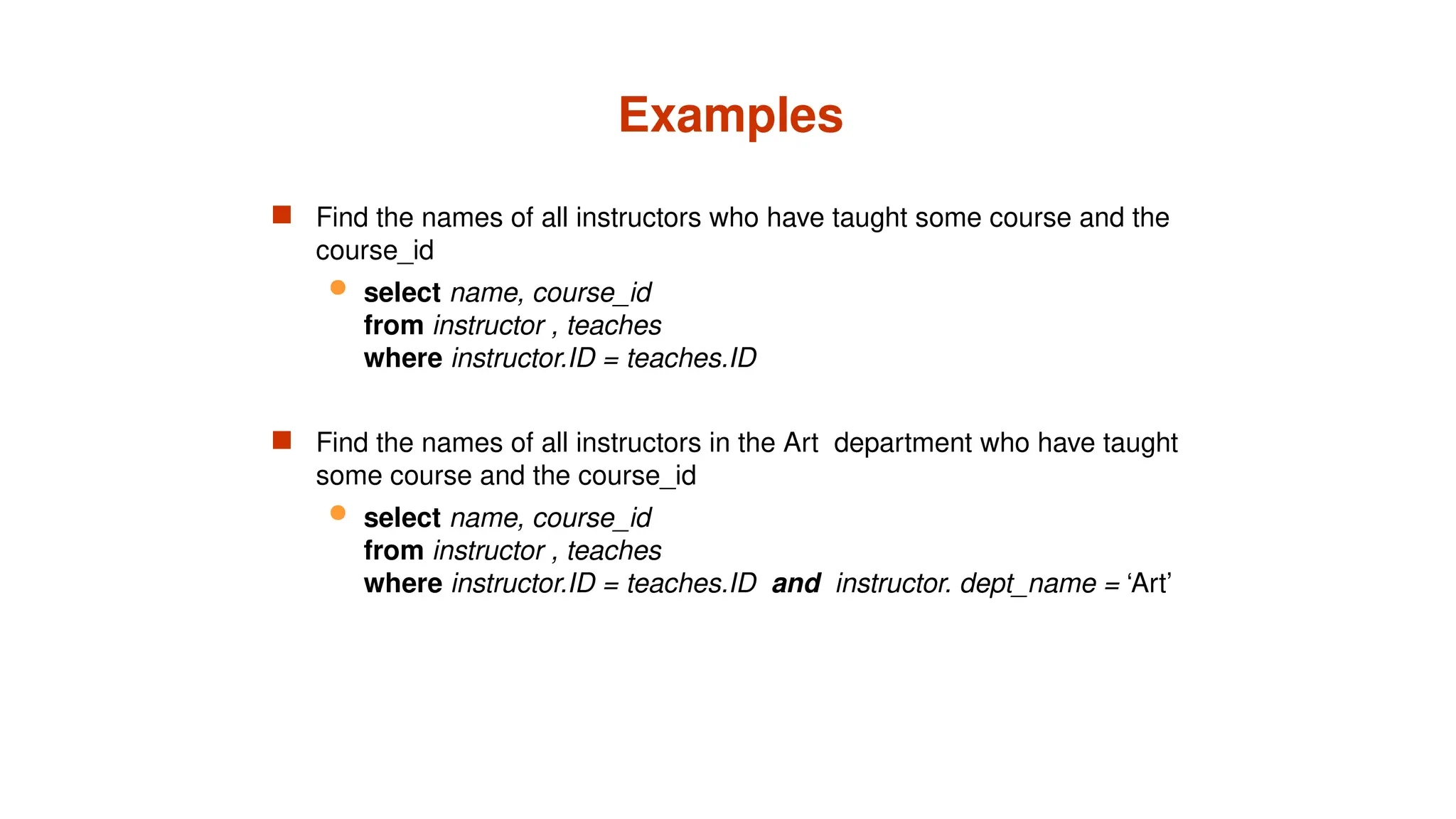
Examples
Find thenames of all instructors who have taught some course and the
course_id
select name, course_id
from instructor , teaches
where instructor.ID = teaches.ID
Find the names of all instructors in the Art department who have taught
some course and the course_id
select name, course_id
from instructor , teaches
where instructor.ID = teaches.ID and instructor. dept_name = ‘Art’
39.
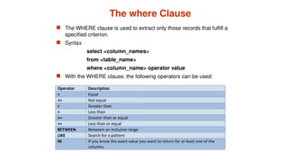
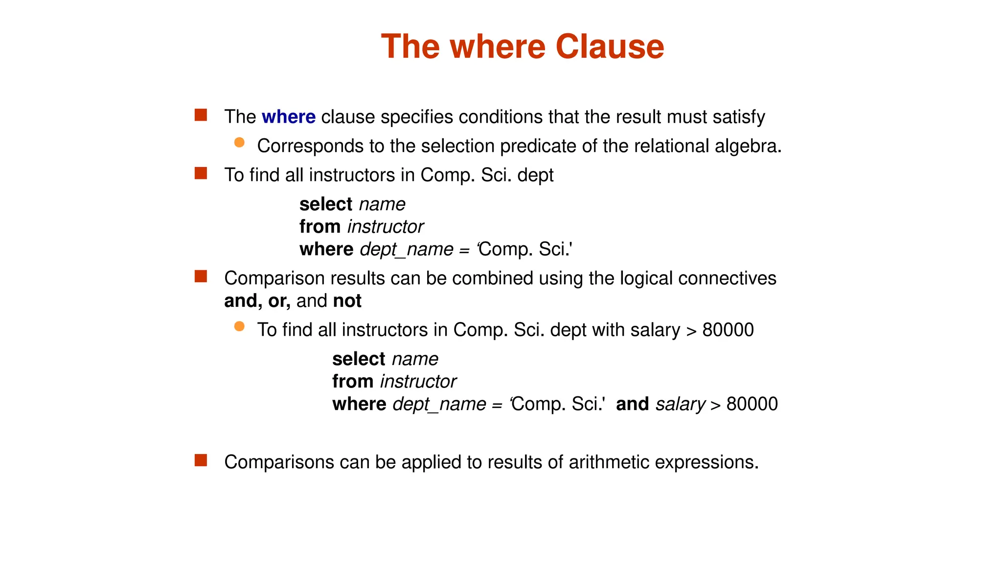
The where Clause
The WHERE clause is used to extract only those records that fulfill a
specified criterion.
Syntax
select <column_names>
from <table_name>
where <column_name> operator value
With the WHERE clause, the following operators can be used:
40.
The where Clause
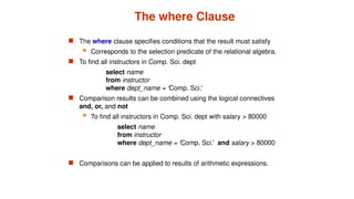
The where clause specifies conditions that the result must satisfy
Corresponds to the selection predicate of the relational algebra.
To find all instructors in Comp. Sci. dept
select name
from instructor
where dept_name = ‘Comp. Sci.'
Comparison results can be combined using the logical connectives
and, or, and not
To find all instructors in Comp. Sci. dept with salary > 80000
select name
from instructor
where dept_name = ‘Comp. Sci.' and salary > 80000
Comparisons can be applied to results of arithmetic expressions.
41.
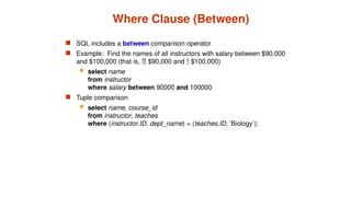
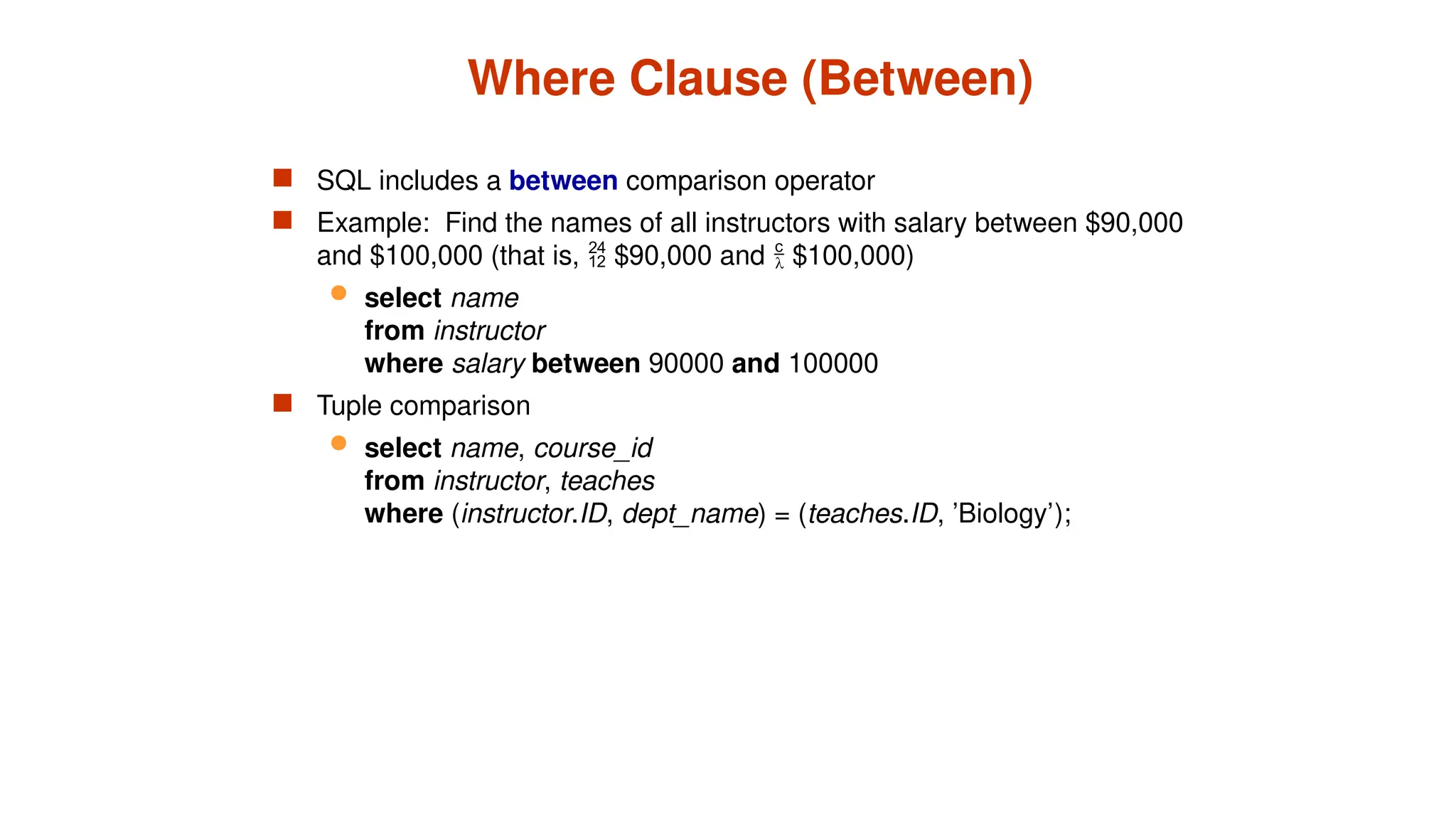
Where Clause (Between)
SQL includes a between comparison operator
Example: Find the names of all instructors with salary between $90,000
and $100,000 (that is, $90,000 and $100,000)
select name
from instructor
where salary between 90000 and 100000
Tuple comparison
select name, course_id
from instructor, teaches
where (instructor.ID, dept_name) = (teaches.ID, ’Biology’);
42.
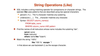
String Operations (Like)
SQL includes a string-matching operator for comparisons on character strings. The
operator like uses patterns that are described using two special characters:
percent ( % ). The % character matches any substring.
underscore ( _ ). The _ character matches any character.
Syntax: SELECT column_name(s)
FROM table_name
WHERE column_name LIKE pattern
Find the names of all instructors whose name includes the substring “dar”.
select name
from instructor
where name like '%dar%'
Match the string “100%”
like ‘100 %' escape ''
in that above we use backslash () as the escape character.
43.
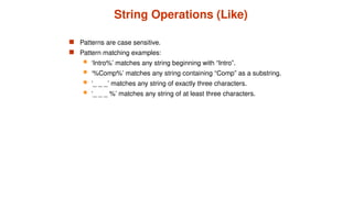
String Operations (Like)
Patterns are case sensitive.
Pattern matching examples:
‘Intro%’ matches any string beginning with “Intro”.
‘%Comp%’ matches any string containing “Comp” as a substring.
‘_ _ _’ matches any string of exactly three characters.
‘_ _ _ %’ matches any string of at least three characters.
44.
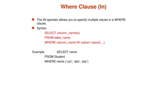
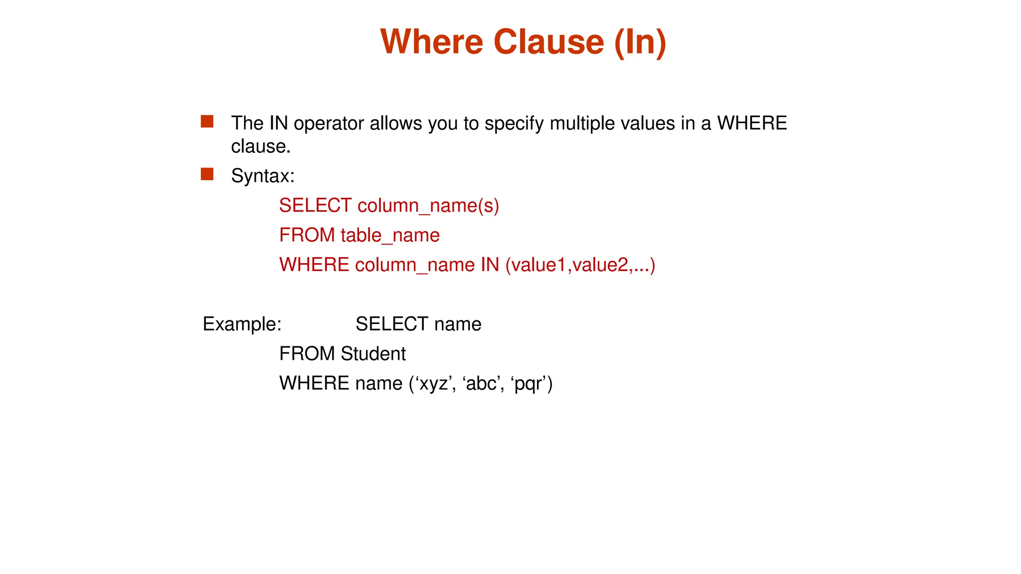
Where Clause (In)
The IN operator allows you to specify multiple values in a WHERE
clause.
Syntax:
SELECT column_name(s)
FROM table_name
WHERE column_name IN (value1,value2,...)
Example: SELECT name
FROM Student
WHERE name (‘xyz’, ‘abc’, ‘pqr’)
45.
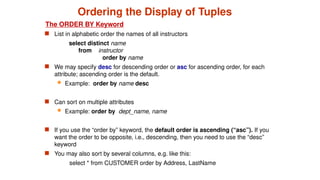
Ordering the Displayof Tuples
The ORDER BY Keyword
List in alphabetic order the names of all instructors
select distinct name
from instructor
order by name
We may specify desc for descending order or asc for ascending order, for each
attribute; ascending order is the default.
Example: order by name desc
Can sort on multiple attributes
Example: order by dept_name, name
If you use the “order by” keyword, the default order is ascending (“asc”). If you
want the order to be opposite, i.e., descending, then you need to use the “desc”
keyword
You may also sort by several columns, e.g. like this:
select * from CUSTOMER order by Address, LastName
46.
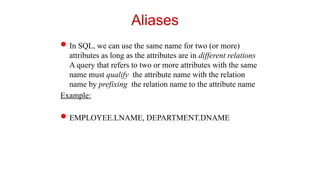
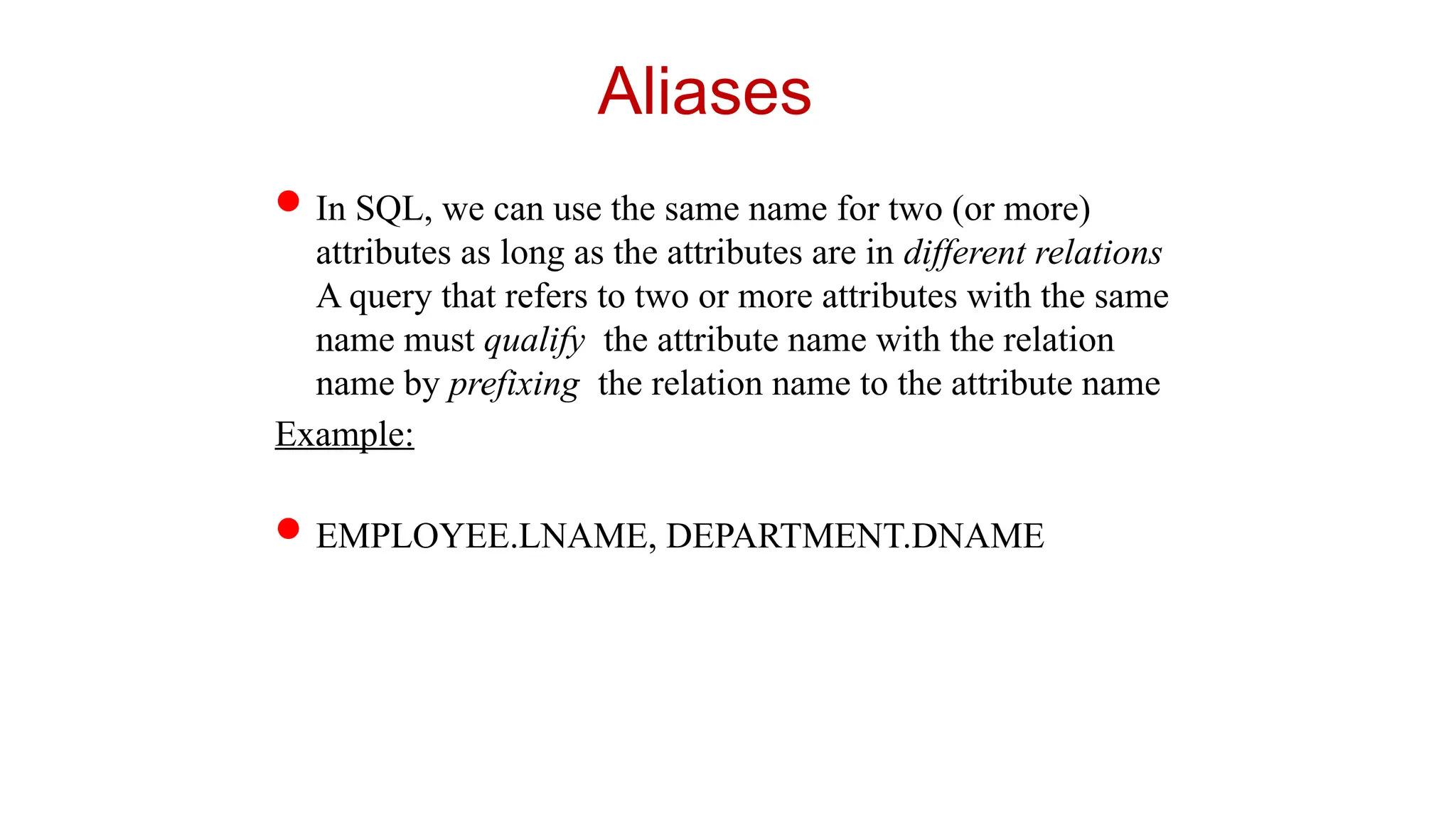
Aliases
In SQL, wecan use the same name for two (or more)
attributes as long as the attributes are in different relations
A query that refers to two or more attributes with the same
name must qualify the attribute name with the relation
name by prefixing the relation name to the attribute name
Example:
EMPLOYEE.LNAME, DEPARTMENT.DNAME
47.
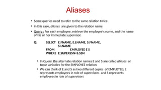
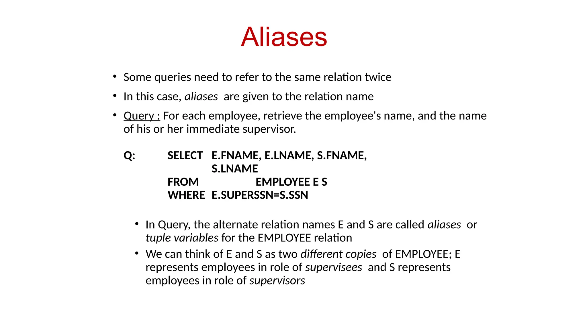
Aliases
• Some queriesneed to refer to the same relation twice
• In this case, aliases are given to the relation name
• Query : For each employee, retrieve the employee's name, and the name
of his or her immediate supervisor.
Q: SELECT E.FNAME, E.LNAME, S.FNAME,
S.LNAME
FROM EMPLOYEE E S
WHERE E.SUPERSSN=S.SSN
• In Query, the alternate relation names E and S are called aliases or
tuple variables for the EMPLOYEE relation
• We can think of E and S as two different copies of EMPLOYEE; E
represents employees in role of supervisees and S represents
employees in role of supervisors
48.
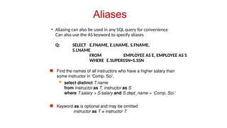
Aliases
• Aliasing canalso be used in any SQL query for convenience
Can also use the AS keyword to specify aliases
Q: SELECT E.FNAME, E.LNAME, S.FNAME,
S.LNAME
FROM EMPLOYEE AS E, EMPLOYEE AS S
WHERE E.SUPERSSN=S.SSN
Find the names of all instructors who have a higher salary than
some instructor in ‘Comp. Sci’.
select distinct T.name
from instructor as T, instructor as S
where T.salary > S.salary and S.dept_name = ‘Comp. Sci.’
Keyword as is optional and may be omitted
instructor as T ≡ instructor T
49.
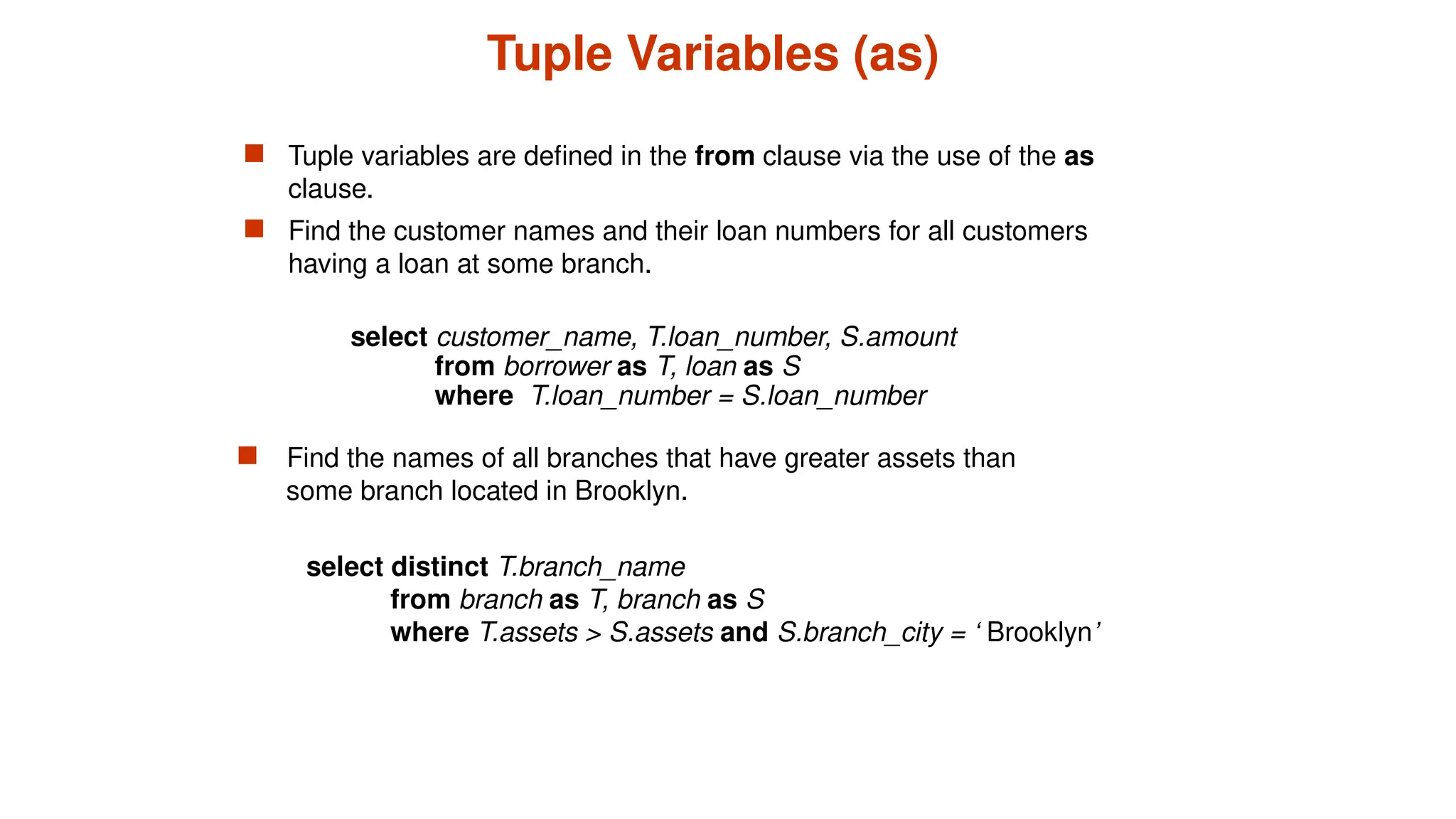
Tuple Variables (as)
Tuple variables are defined in the from clause via the use of the as
clause.
Find the customer names and their loan numbers for all customers
having a loan at some branch.
select distinct T.branch_name
from branch as T, branch as S
where T.assets > S.assets and S.branch_city = ‘ Brooklyn’
Find the names of all branches that have greater assets than
some branch located in Brooklyn.
select customer_name, T.loan_number, S.amount
from borrower as T, loan as S
where T.loan_number = S.loan_number
50.
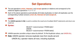
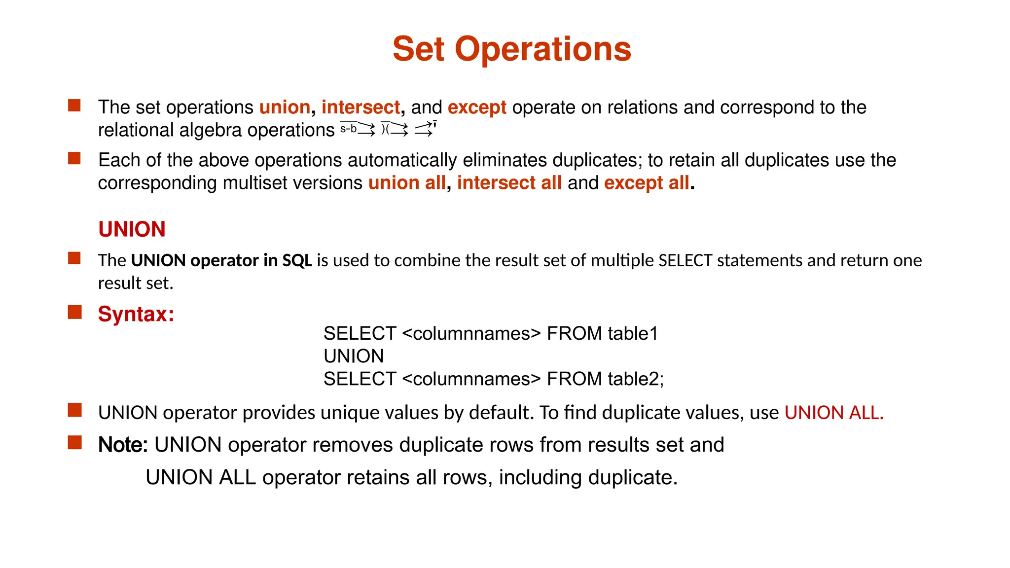
Set Operations
Theset operations union, intersect, and except operate on relations and correspond to the
relational algebra operations
Each of the above operations automatically eliminates duplicates; to retain all duplicates use the
corresponding multiset versions union all, intersect all and except all.
UNION
The UNION operator in SQL is used to combine the result set of multiple SELECT statements and return one
result set.
Syntax:
UNION operator provides unique values by default. To find duplicate values, use UNION ALL.
Note: UNION operator removes duplicate rows from results set and
UNION ALL operator retains all rows, including duplicate.
SELECT <columnnames> FROM table1
UNION
SELECT <columnnames> FROM table2;
51.
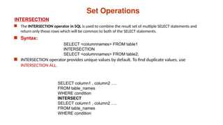
Set Operations
INTERSECTION
TheINTERSECTION operator in SQL is used to combine the result set of multiple SELECT statements and
return only those rows which will be common to both of the SELECT statements.
Syntax:
INTERSECTION operator provides unique values by default. To find duplicate values, use
INTERSECTION ALL.
SELECT <columnnames> FROM table1
INTERSECTION
SELECT <columnnames> FROM table2;
SELECT column1 , column2 ….
FROM table_names
WHERE condition
INTERSECT
SELECT column1 , column2 ….
FROM table_names
WHERE condition
52.
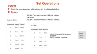
Set Operations
EXCEPT
Thisis the same as using a subtract operator in relational algebra.
Syntax:
SELECT <columnnames> FROM table1
EXCEPT
SELECT <columnnames> FROM table2;
SELECT Name FROM Students
EXCEPT
SELECT NAME FROM TA;
53.
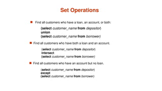
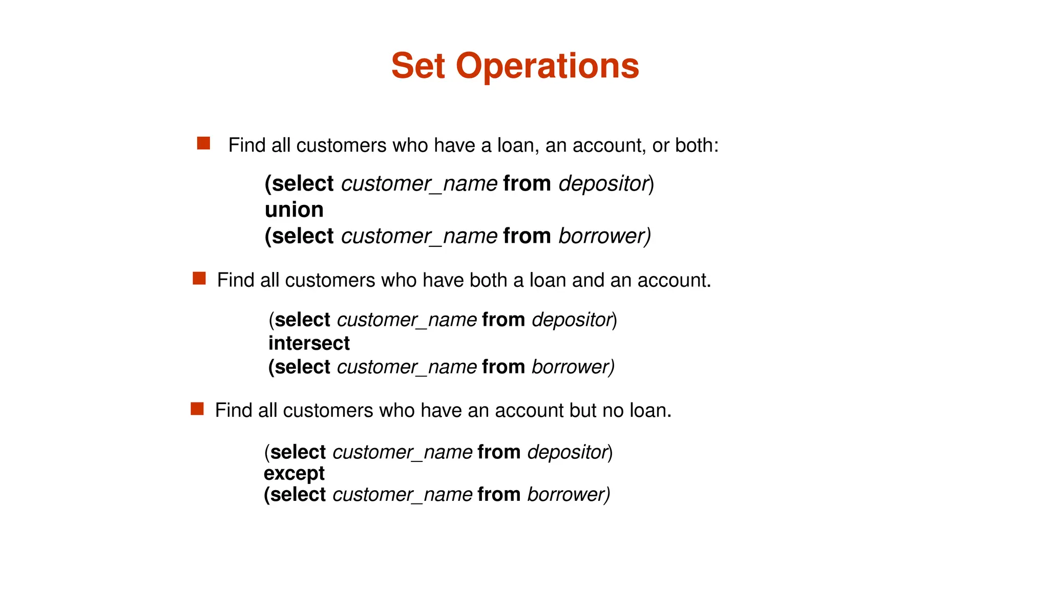
Set Operations
Findall customers who have a loan, an account, or both:
(select customer_name from depositor)
except
(select customer_name from borrower)
(select customer_name from depositor)
intersect
(select customer_name from borrower)
Find all customers who have an account but no loan.
(select customer_name from depositor)
union
(select customer_name from borrower)
Find all customers who have both a loan and an account.
54.
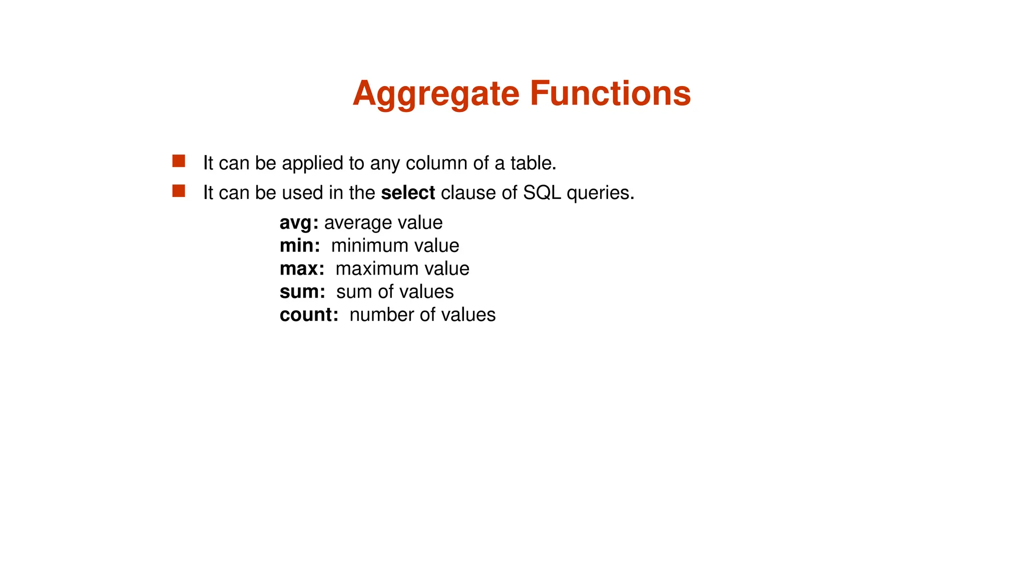
Aggregate Functions
Itcan be applied to any column of a table.
It can be used in the select clause of SQL queries.
avg: average value
min: minimum value
max: maximum value
sum: sum of values
count: number of values
55.
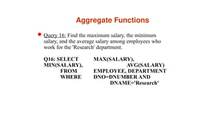
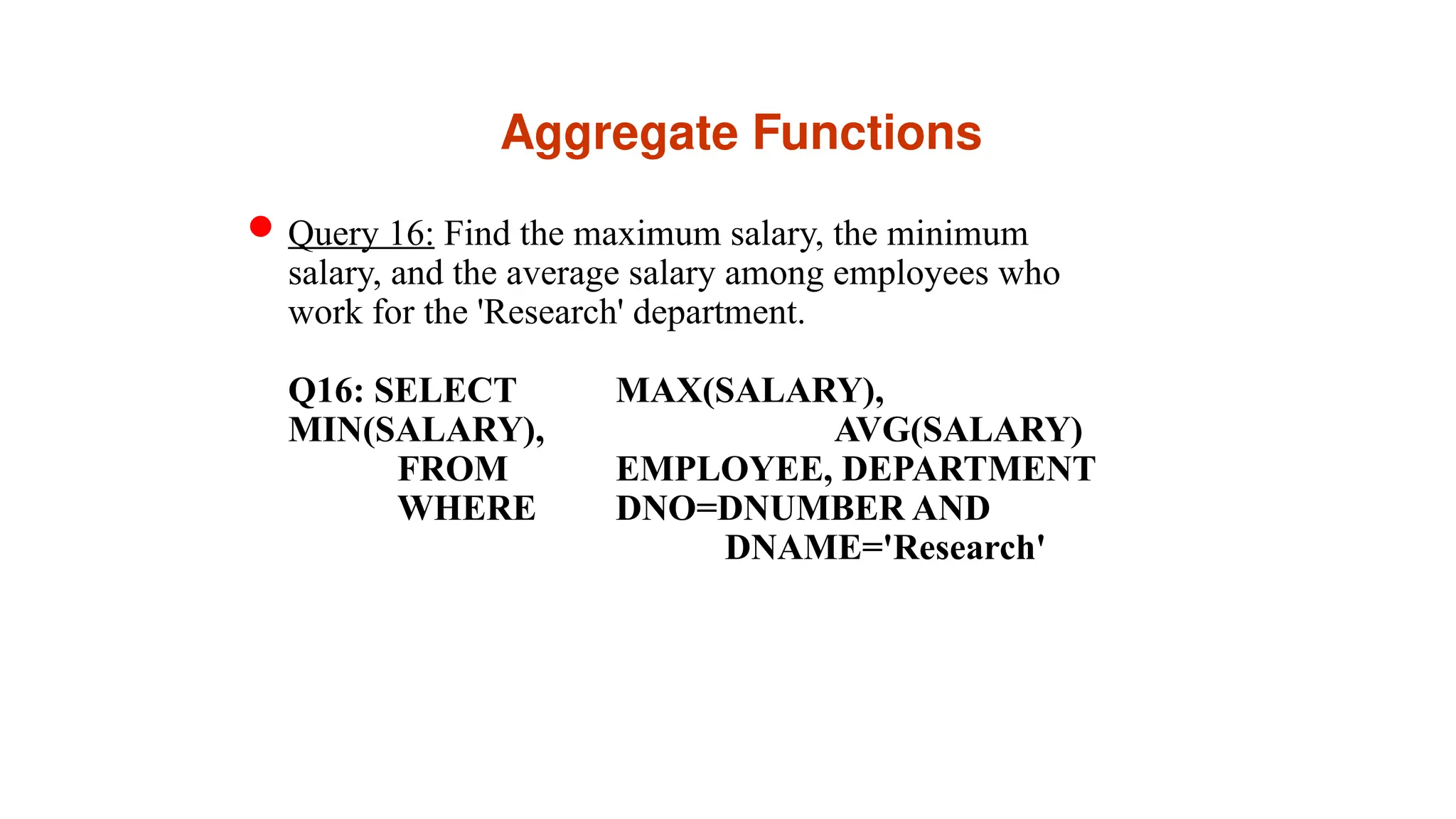
Aggregate Functions
Query 16:Find the maximum salary, the minimum
salary, and the average salary among employees who
work for the 'Research' department.
Q16: SELECT MAX(SALARY),
MIN(SALARY), AVG(SALARY)
FROM EMPLOYEE, DEPARTMENT
WHERE DNO=DNUMBER AND
DNAME='Research'
56.
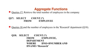
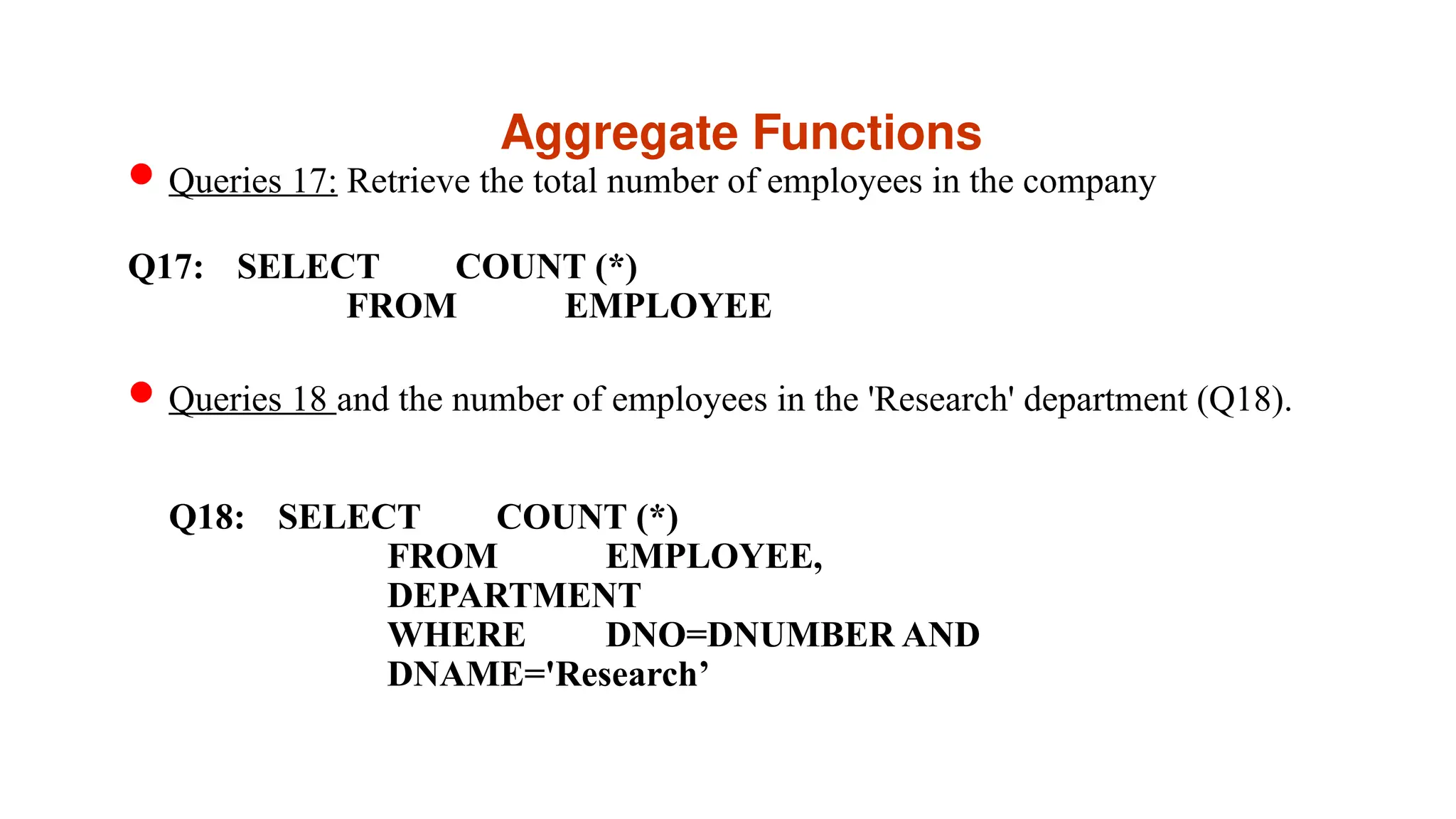
Aggregate Functions
Queries 17:Retrieve the total number of employees in the company
Q17: SELECT COUNT (*)
FROM EMPLOYEE
Queries 18 and the number of employees in the 'Research' department (Q18).
Q18: SELECT COUNT (*)
FROM EMPLOYEE,
DEPARTMENT
WHERE DNO=DNUMBER AND
DNAME='Research’
57.
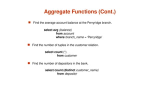
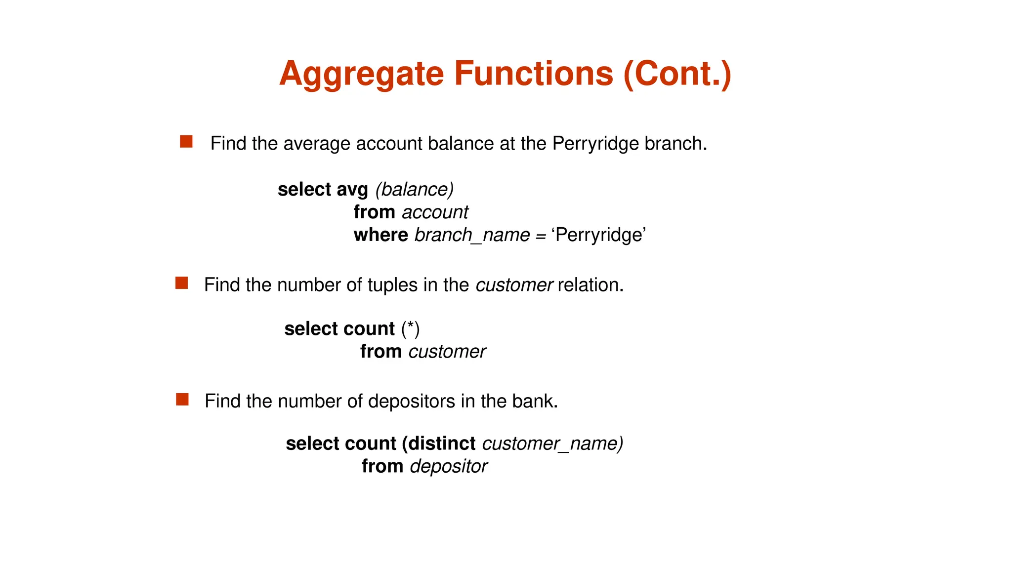
Aggregate Functions (Cont.)
Find the average account balance at the Perryridge branch.
Find the number of depositors in the bank.
Find the number of tuples in the customer relation.
select avg (balance)
from account
where branch_name = ‘Perryridge’
select count (*)
from customer
select count (distinct customer_name)
from depositor
58.
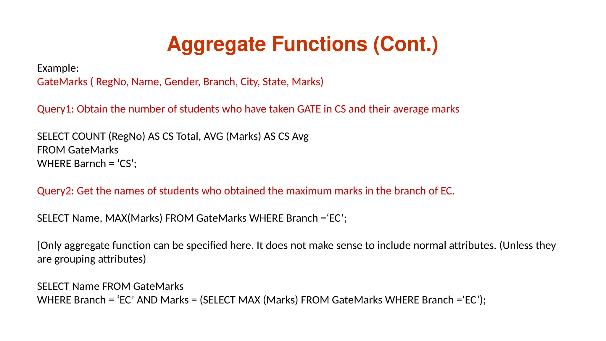
Aggregate Functions (Cont.)
Example:
GateMarks( RegNo, Name, Gender, Branch, City, State, Marks)
Query1: Obtain the number of students who have taken GATE in CS and their average marks
SELECT COUNT (RegNo) AS CS Total, AVG (Marks) AS CS Avg
FROM GateMarks
WHERE Barnch = ‘CS’;
Query2: Get the names of students who obtained the maximum marks in the branch of EC.
SELECT Name, MAX(Marks) FROM GateMarks WHERE Branch =‘EC’;
[Only aggregate function can be specified here. It does not make sense to include normal attributes. (Unless they
are grouping attributes)
SELECT Name FROM GateMarks
WHERE Branch = ‘EC’ AND Marks = (SELECT MAX (Marks) FROM GateMarks WHERE Branch =‘EC’);
59.
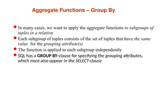
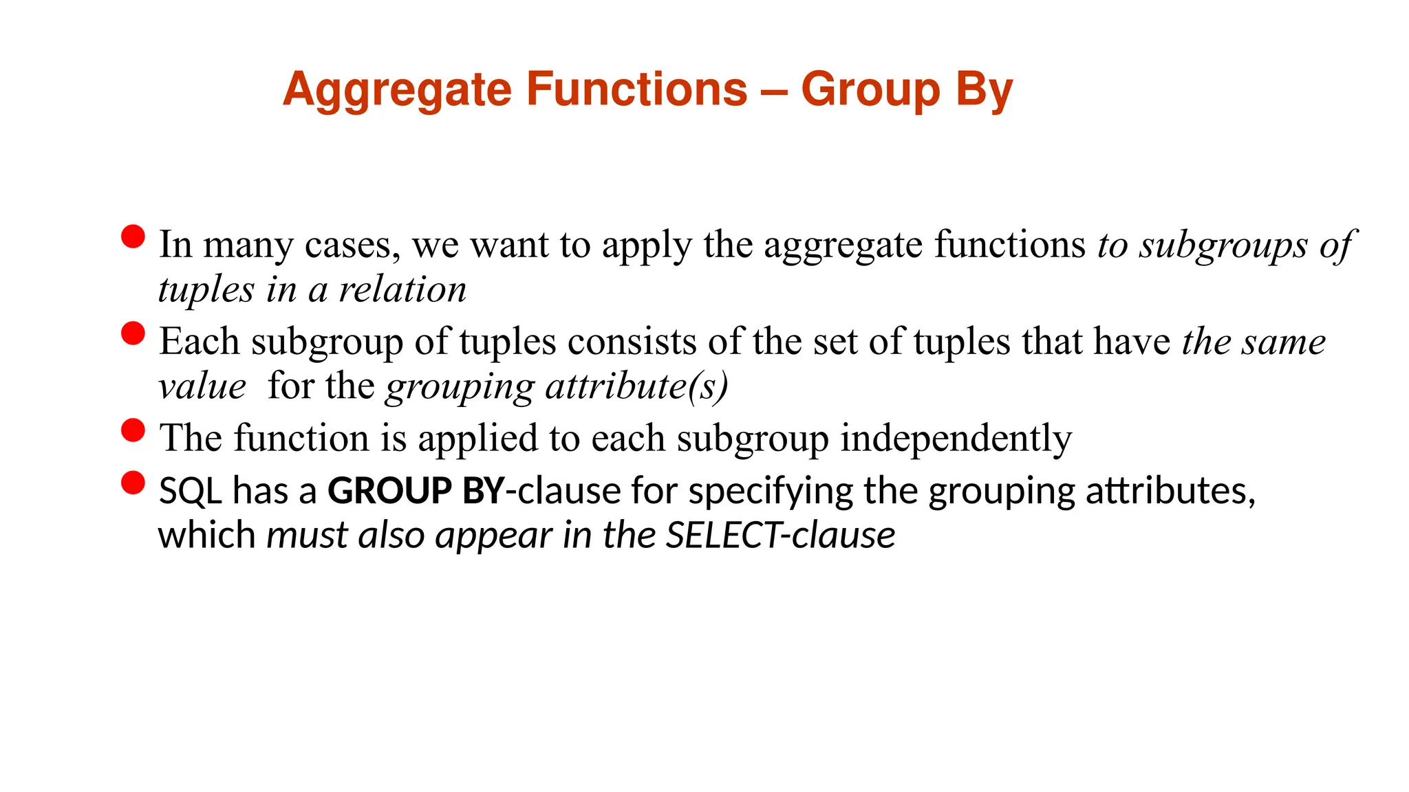
Aggregate Functions –Group By
In many cases, we want to apply the aggregate functions to subgroups of
tuples in a relation
Each subgroup of tuples consists of the set of tuples that have the same
value for the grouping attribute(s)
The function is applied to each subgroup independently
SQL has a GROUP BY-clause for specifying the grouping attributes,
which must also appear in the SELECT-clause
60.
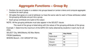
Aggregate Functions –Group By
Partition the set of tuples in a relation into groups based on certain criteria and compute aggregate
functions for each group.
All tuples that agree on a set of attribute (i.e have the same vale for each of these attributes) called
the grouping attributes are put into a group.
Each group contribute one tuple to the output.
NOTE: All the grouping attributes must also appear in the SELECT clause.
The result of the group is listed along with the values of the grouping attributes of the group.
Example 1: Determine the maximum of the GATE CS marks obtained by students in each city for all
cities.
SELECT City, MAX(Marks) AS Max Marks
FROM GateMarks
WHERE Branch =‘CS’ GROUP BY City;
City Max Marks
Hyderabad 87
Chennai 84
Mysore 90
Bangalore 82
61.
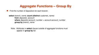
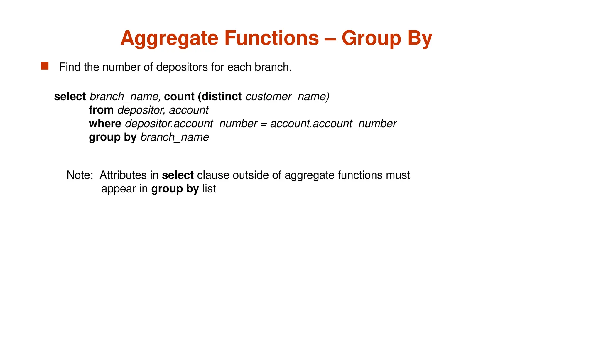
Aggregate Functions –Group By
Find the number of depositors for each branch.
Note: Attributes in select clause outside of aggregate functions must
appear in group by list
select branch_name, count (distinct customer_name)
from depositor, account
where depositor.account_number = account.account_number
group by branch_name
62.
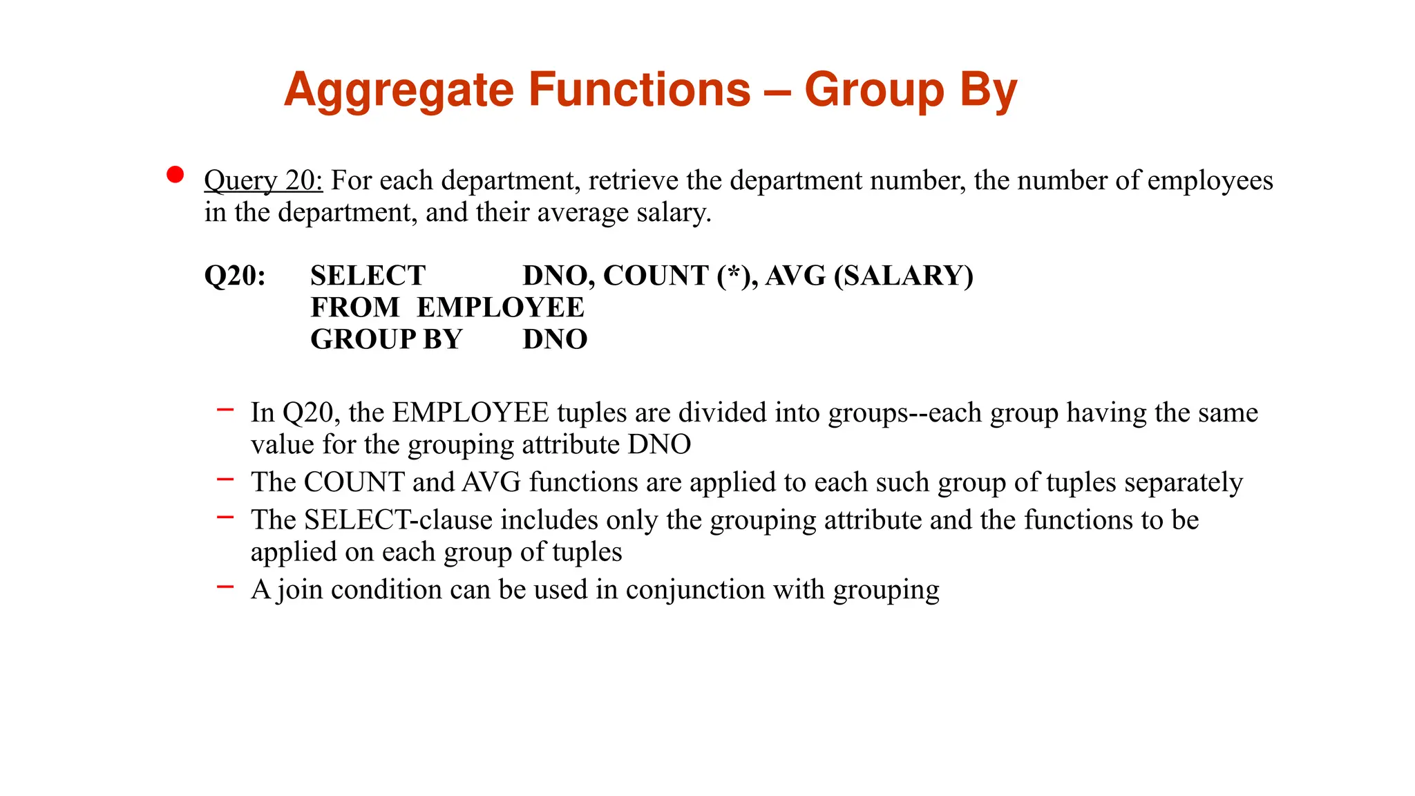
Aggregate Functions –Group By
Query 20: For each department, retrieve the department number, the number of employees
in the department, and their average salary.
Q20: SELECT DNO, COUNT (*), AVG (SALARY)
FROM EMPLOYEE
GROUP BY DNO
– In Q20, the EMPLOYEE tuples are divided into groups--each group having the same
value for the grouping attribute DNO
– The COUNT and AVG functions are applied to each such group of tuples separately
– The SELECT-clause includes only the grouping attribute and the functions to be
applied on each group of tuples
– A join condition can be used in conjunction with grouping
63.
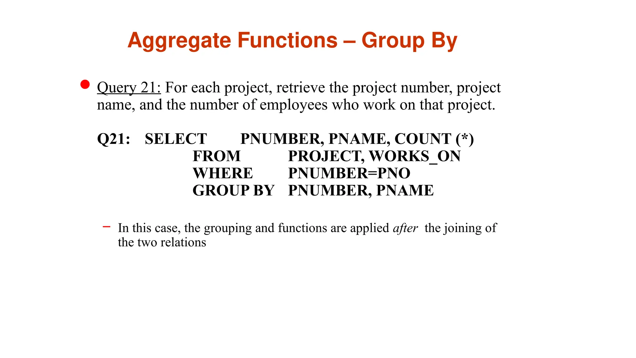
Aggregate Functions –Group By
Query 21: For each project, retrieve the project number, project
name, and the number of employees who work on that project.
Q21: SELECT PNUMBER, PNAME, COUNT (*)
FROM PROJECT, WORKS_ON
WHERE PNUMBER=PNO
GROUP BY PNUMBER, PNAME
– In this case, the grouping and functions are applied after the joining of
the two relations
64.
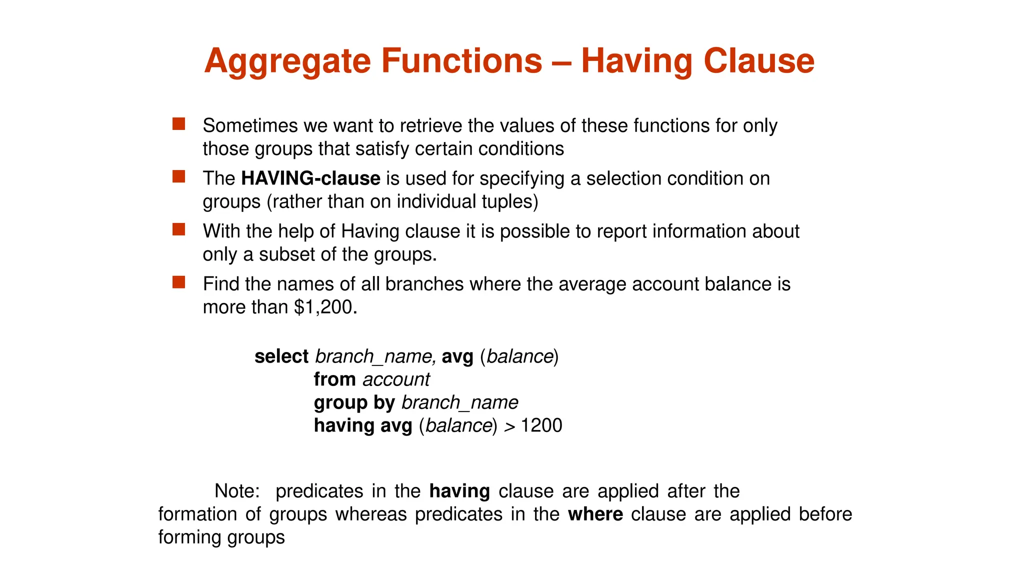
Aggregate Functions –Having Clause
Sometimes we want to retrieve the values of these functions for only
those groups that satisfy certain conditions
The HAVING-clause is used for specifying a selection condition on
groups (rather than on individual tuples)
With the help of Having clause it is possible to report information about
only a subset of the groups.
Find the names of all branches where the average account balance is
more than $1,200.
Note: predicates in the having clause are applied after the
formation of groups whereas predicates in the where clause are applied before
forming groups
select branch_name, avg (balance)
from account
group by branch_name
having avg (balance) > 1200
65.
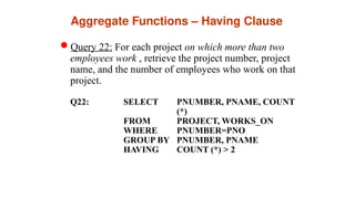
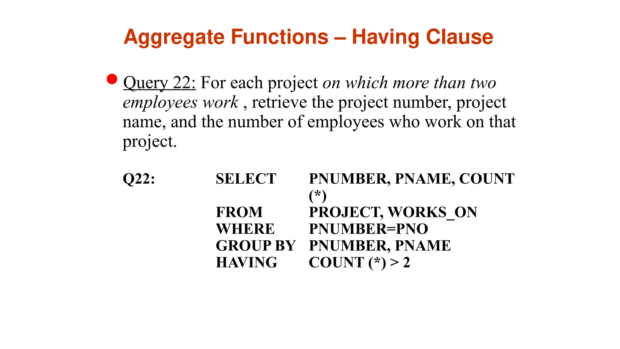
Aggregate Functions –Having Clause
Query 22: For each project on which more than two
employees work , retrieve the project number, project
name, and the number of employees who work on that
project.
Q22: SELECT PNUMBER, PNAME, COUNT
(*)
FROM PROJECT, WORKS_ON
WHERE PNUMBER=PNO
GROUP BY PNUMBER, PNAME
HAVING COUNT (*) > 2
66.
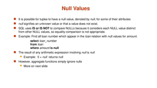
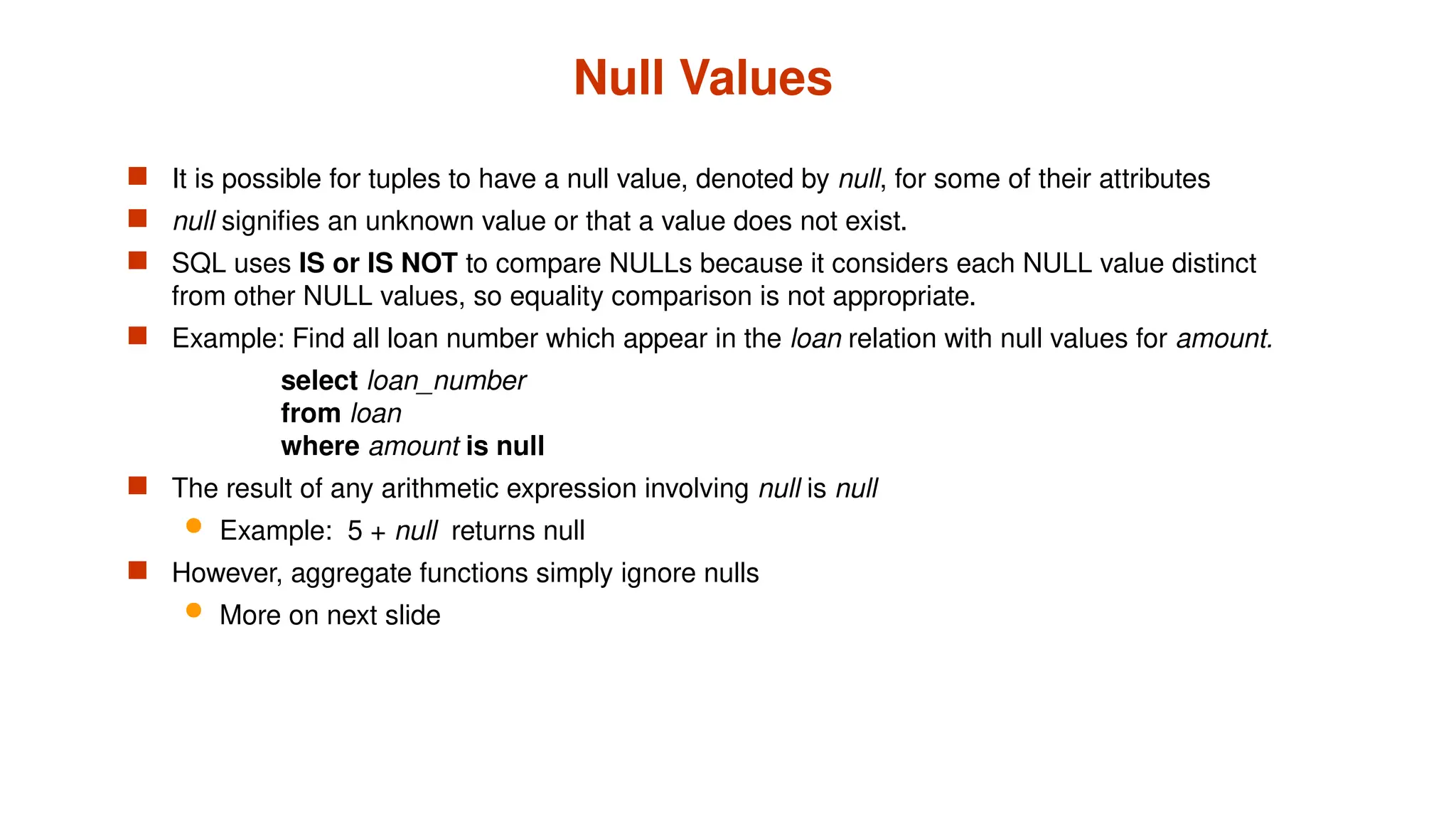
Null Values
Itis possible for tuples to have a null value, denoted by null, for some of their attributes
null signifies an unknown value or that a value does not exist.
SQL uses IS or IS NOT to compare NULLs because it considers each NULL value distinct
from other NULL values, so equality comparison is not appropriate.
Example: Find all loan number which appear in the loan relation with null values for amount.
select loan_number
from loan
where amount is null
The result of any arithmetic expression involving null is null
Example: 5 + null returns null
However, aggregate functions simply ignore nulls
More on next slide
67.
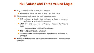
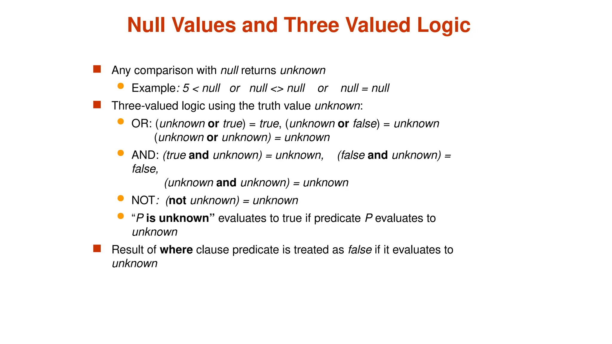
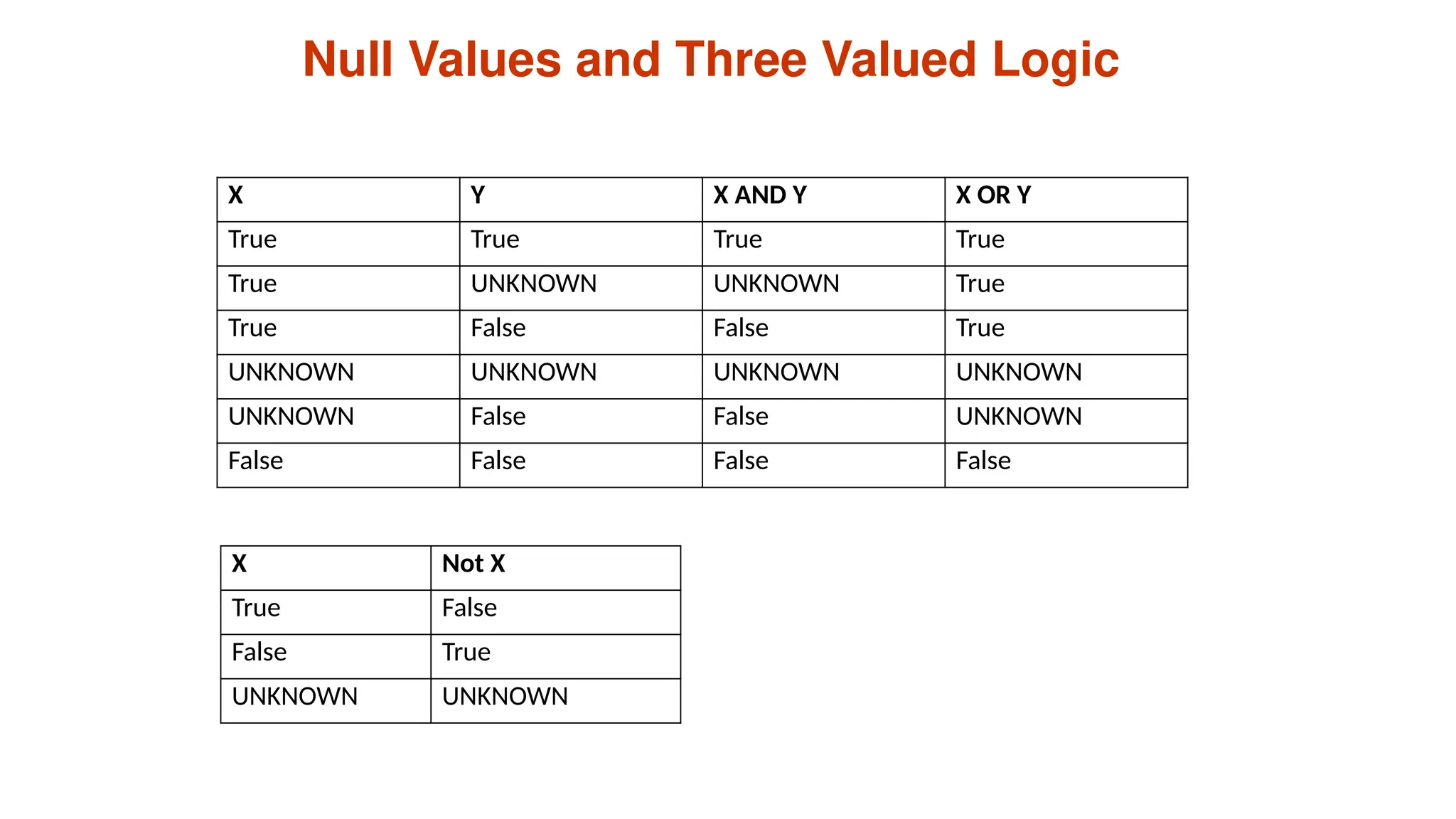
Null Values andThree Valued Logic
Any comparison with null returns unknown
Example: 5 < null or null <> null or null = null
Three-valued logic using the truth value unknown:
OR: (unknown or true) = true, (unknown or false) = unknown
(unknown or unknown) = unknown
AND: (true and unknown) = unknown, (false and unknown) =
false,
(unknown and unknown) = unknown
NOT: (not unknown) = unknown
“P is unknown” evaluates to true if predicate P evaluates to
unknown
Result of where clause predicate is treated as false if it evaluates to
unknown
68.
Null Values andThree Valued Logic
X Y X AND Y X OR Y
True True True True
True UNKNOWN UNKNOWN True
True False False True
UNKNOWN UNKNOWN UNKNOWN UNKNOWN
UNKNOWN False False UNKNOWN
False False False False
X Not X
True False
False True
UNKNOWN UNKNOWN
69.
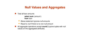
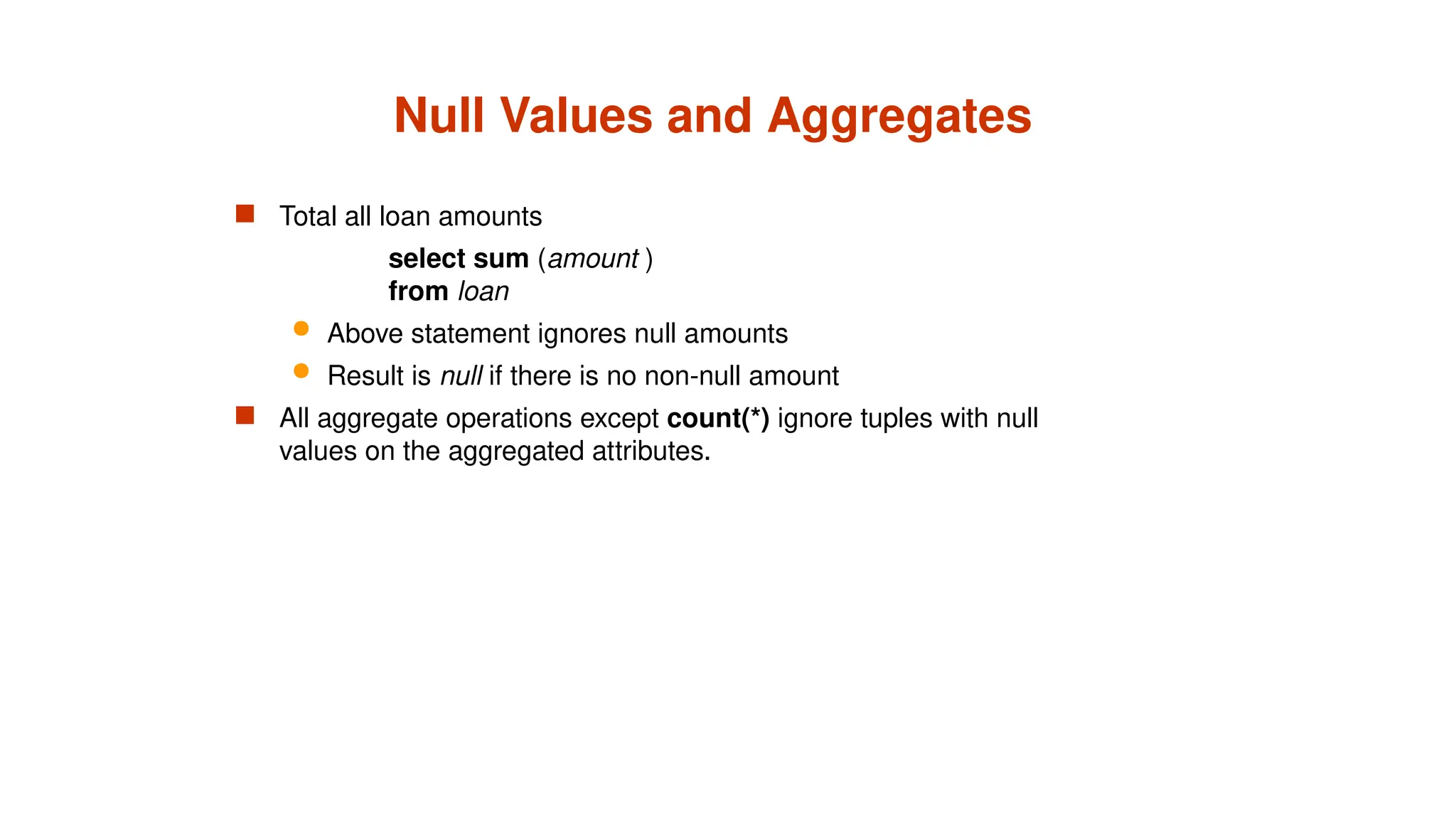
Null Values andAggregates
Total all loan amounts
select sum (amount )
from loan
Above statement ignores null amounts
Result is null if there is no non-null amount
All aggregate operations except count(*) ignore tuples with null
values on the aggregated attributes.
70.
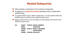
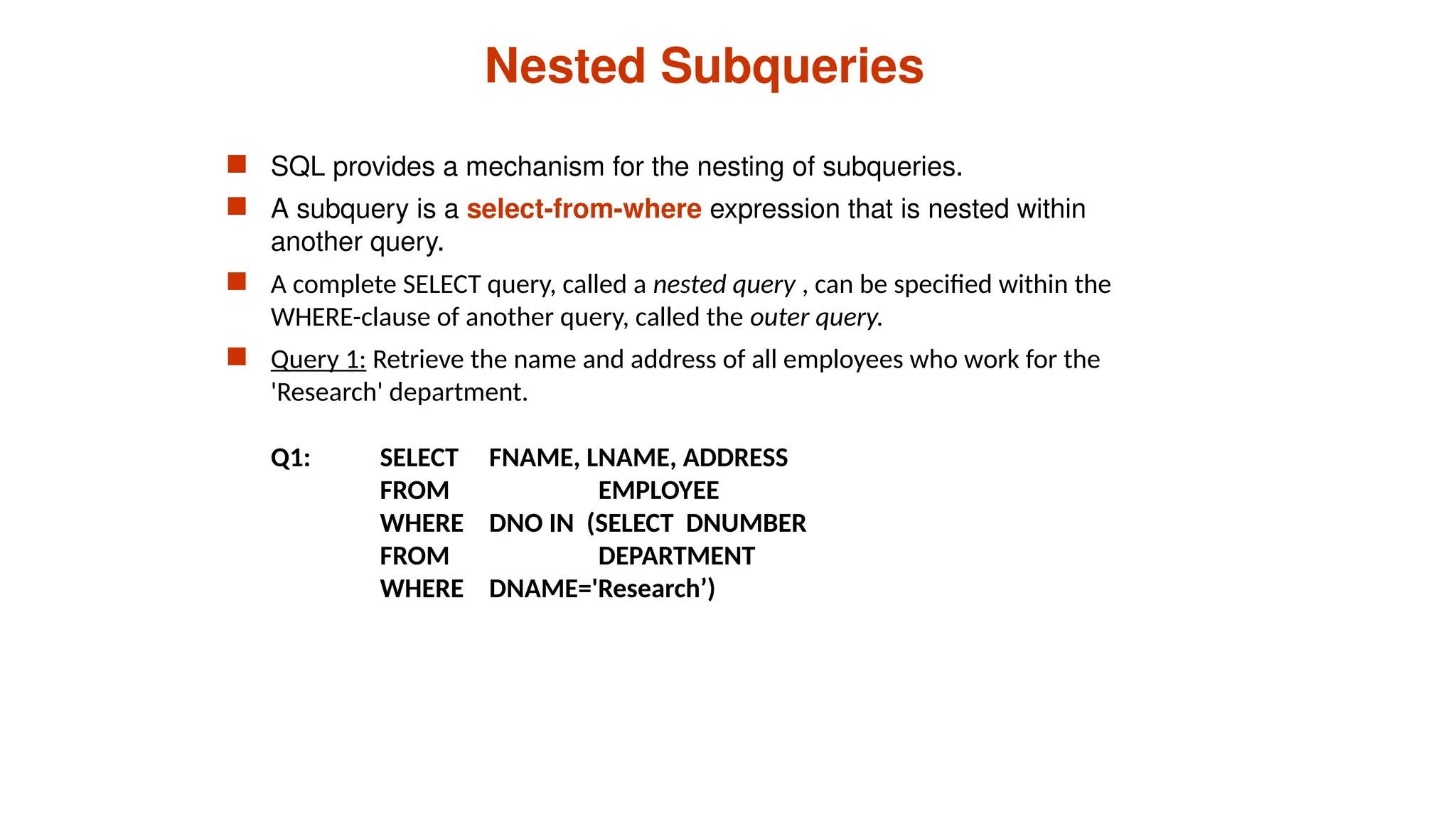
Nested Subqueries
SQLprovides a mechanism for the nesting of subqueries.
A subquery is a select-from-where expression that is nested within
another query.
A complete SELECT query, called a nested query , can be specified within the
WHERE-clause of another query, called the outer query.
Query 1: Retrieve the name and address of all employees who work for the
'Research' department.
Q1: SELECT FNAME, LNAME, ADDRESS
FROM EMPLOYEE
WHERE DNO IN (SELECT DNUMBER
FROM DEPARTMENT
WHERE DNAME='Research’)
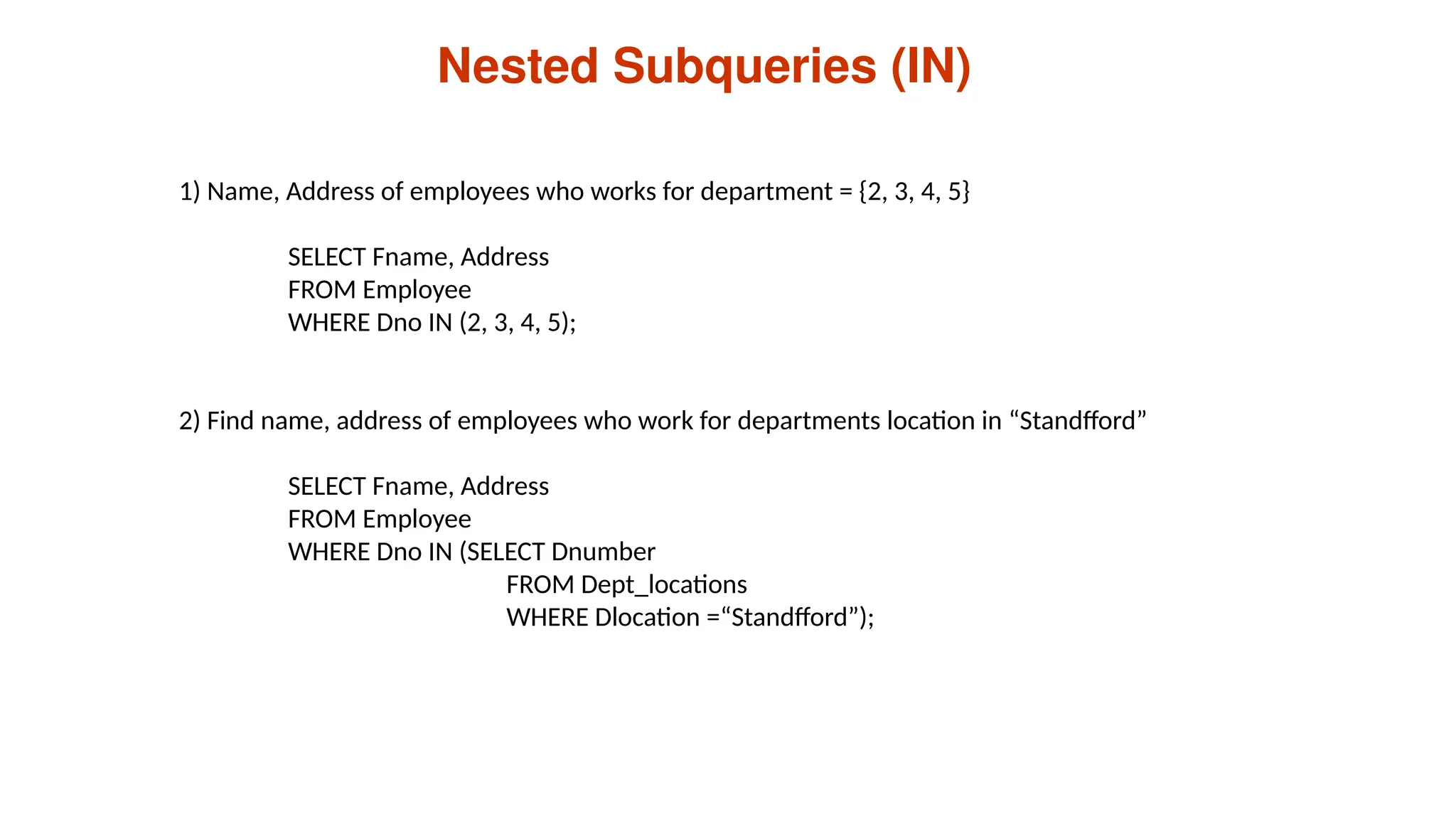
Nested Subqueries (IN)
1)Name, Address of employees who works for department = {2, 3, 4, 5}
SELECT Fname, Address
FROM Employee
WHERE Dno IN (2, 3, 4, 5);
2) Find name, address of employees who work for departments location in “Standfford”
SELECT Fname, Address
FROM Employee
WHERE Dno IN (SELECT Dnumber
FROM Dept_locations
WHERE Dlocation =“Standfford”);
73.
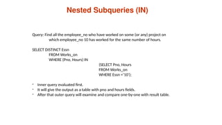
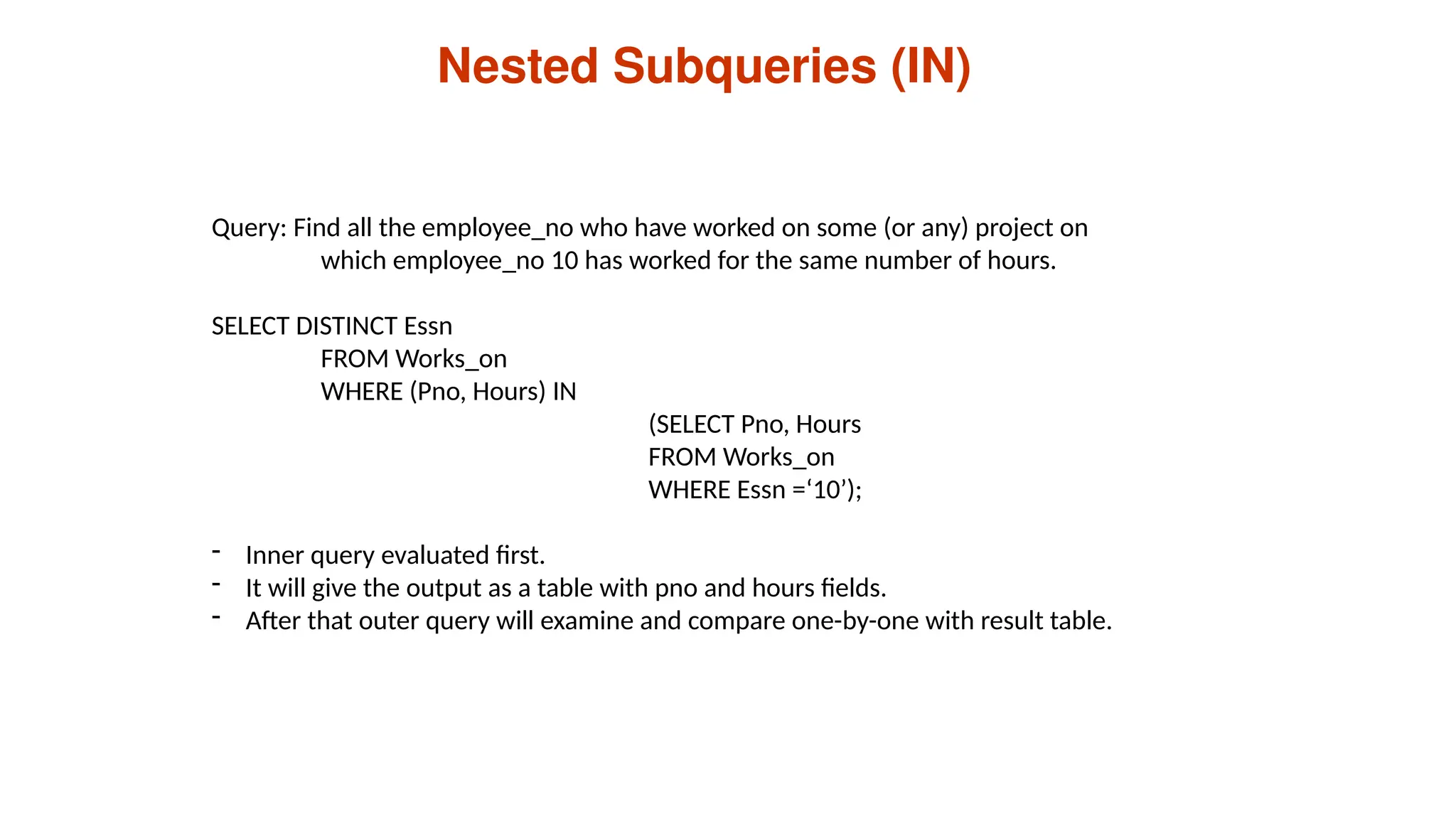
Nested Subqueries (IN)
Query:Find all the employee_no who have worked on some (or any) project on
which employee_no 10 has worked for the same number of hours.
SELECT DISTINCT Essn
FROM Works_on
WHERE (Pno, Hours) IN
(SELECT Pno, Hours
FROM Works_on
WHERE Essn =‘10’);
- Inner query evaluated first.
- It will give the output as a table with pno and hours fields.
- After that outer query will examine and compare one-by-one with result table.
74.
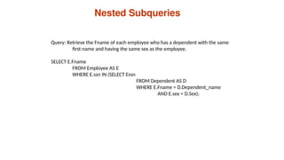
Nested Subqueries
Query: Retrievethe Fname of each employee who has a dependent with the same
first name and having the same sex as the employee.
SELECT E.Fname
FROM Employee AS E
WHERE E.ssn IN (SELECT Essn
FROM Dependent AS D
WHERE E.Fname = D.Dependent_name
AND E.sex = D.Sex);
75.
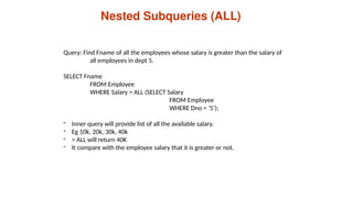
Nested Subqueries (ALL)
Query:Find Fname of all the employees whose salary is greater than the salary of
all employees in dept 5.
SELECT Fname
FROM Employee
WHERE Salary > ALL (SELECT Salary
FROM Employee
WHERE Dno = ‘5’);
- Inner query will provide list of all the available salary.
- Eg 10k, 20k, 30k, 40k
- > ALL will return 40K
- It compare with the employee salary that it is greater or not.
76.
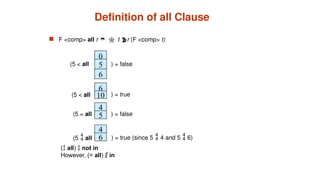
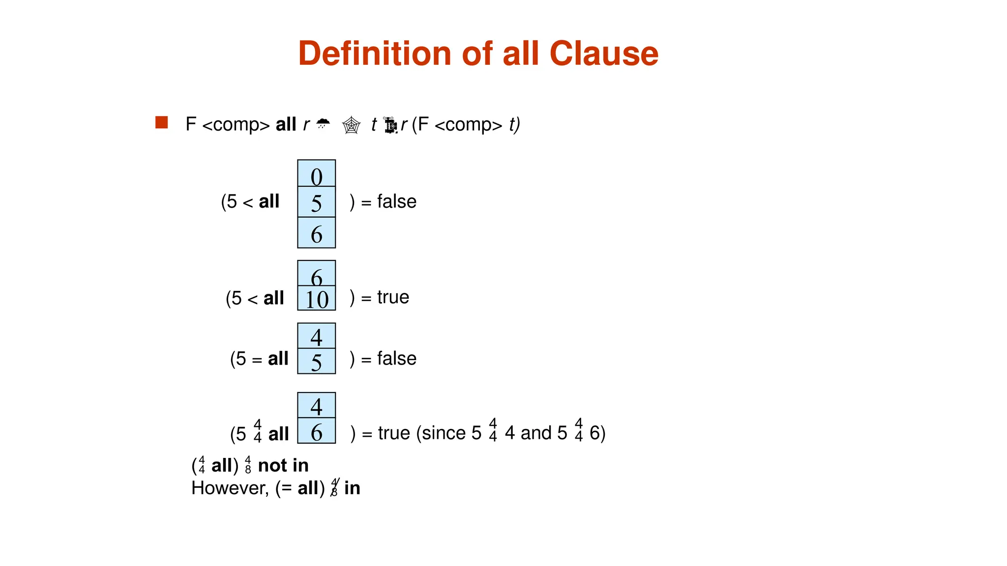
Definition of allClause
F <comp> all r t r (F <comp> t)
0
5
6
(5 < all ) = false
6
10
4
) = true
5
4
6
(5 all ) = true (since 5 4 and 5 6)
(5 < all
) = false
(5 = all
( all) not in
However, (= all) in
77.
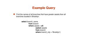
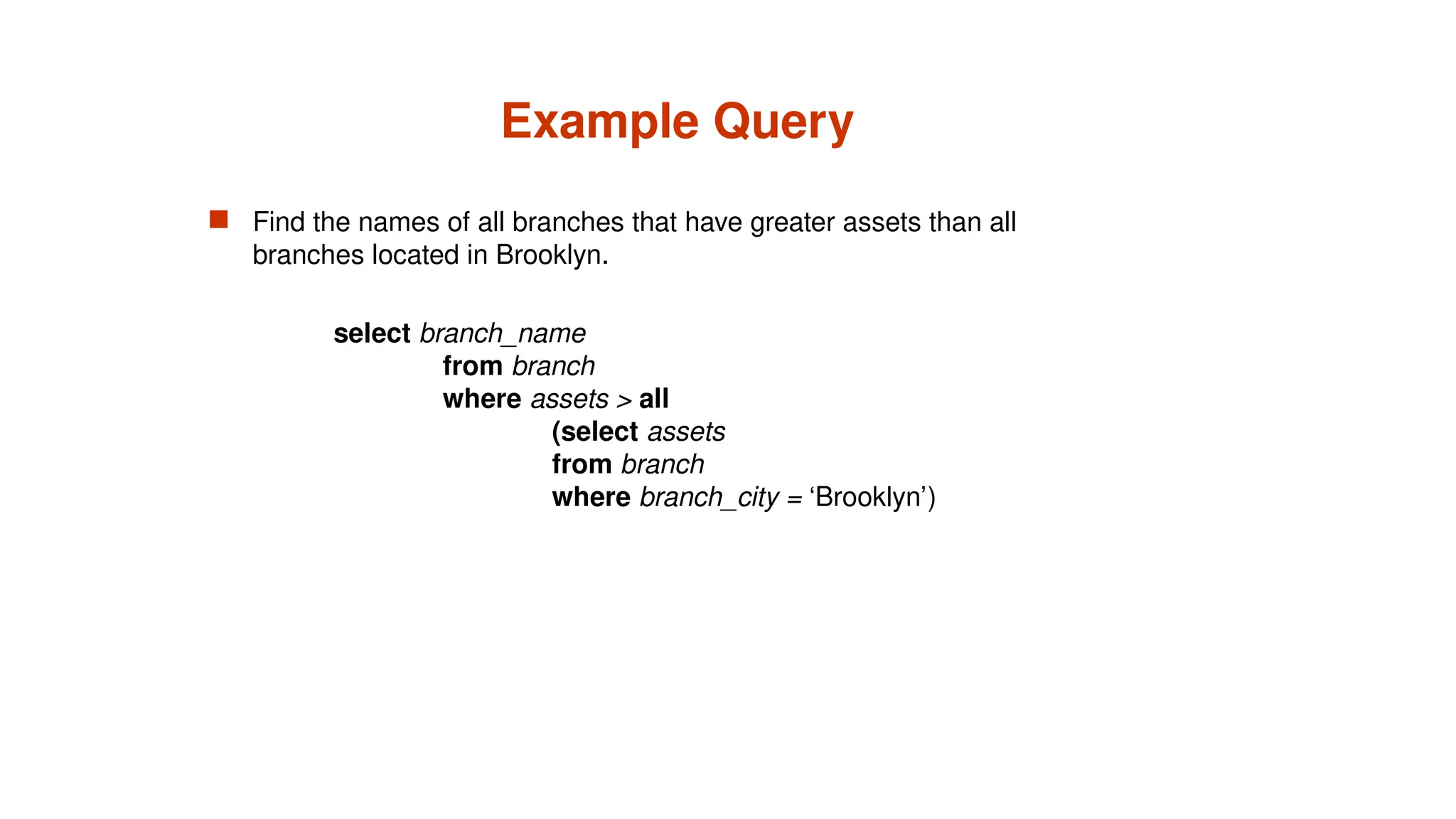
Example Query
Findthe names of all branches that have greater assets than all
branches located in Brooklyn.
select branch_name
from branch
where assets > all
(select assets
from branch
where branch_city = ‘Brooklyn’)
78.
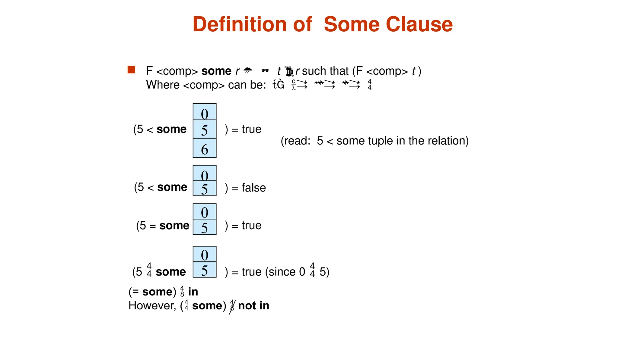
Definition of SomeClause
F <comp> some r t r such that (F <comp> t )
Where <comp> can be:
0
5
6
(5 < some ) = true
0
5
0
) = false
5
0
5
(5 some ) = true (since 0 5)
(read: 5 < some tuple in the relation)
(5 < some
) = true
(5 = some
(= some) in
However, ( some) not in
79.
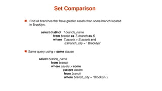
Set Comparison
Findall branches that have greater assets than some branch located
in Brooklyn.
Same query using > some clause
select branch_name
from branch
where assets > some
(select assets
from branch
where branch_city = ‘Brooklyn’)
select distinct T.branch_name
from branch as T, branch as S
where T.assets > S.assets and
S.branch_city = ‘ Brooklyn’
80.
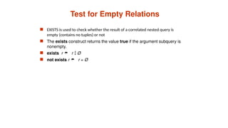
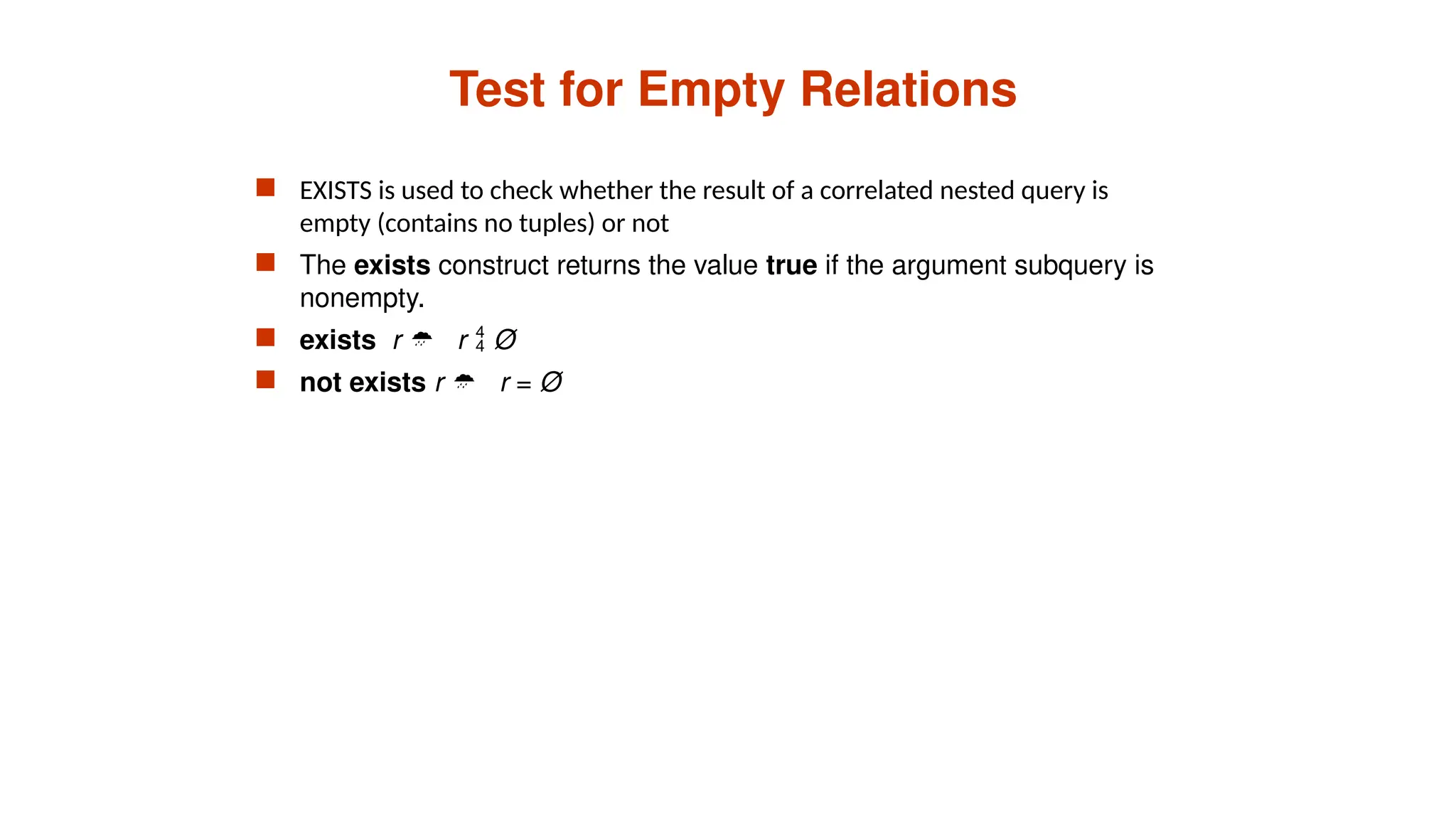
Test for EmptyRelations
EXISTS is used to check whether the result of a correlated nested query is
empty (contains no tuples) or not
The exists construct returns the value true if the argument subquery is
nonempty.
exists r r Ø
not exists r r = Ø
81.
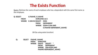
Query: Retrieve thename of each employee who has a dependent with the same first name as
the employee.
Q: SELECT E.FNAME, E.LNAME
FROM EMPLOYEE AS E
WHERE E.SSN IN (SELECT ESSN
FROM DEPENDENT
WHERE ESSN=E.SSN AND
E.FNAME=DEPENDENT_NAME)
The Exists Function
Q: SELECT FNAME, LNAME
FROM EMPLOYEE
WHERE EXISTS (SELECT *
FROM DEPENDENT
WHERE SSN=ESSN AND
FNAME=DEPENDENT_NAME)
OR (by using exists function)
82.
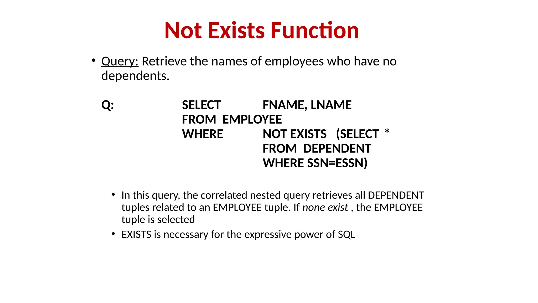
• Query: Retrievethe names of employees who have no
dependents.
Q: SELECT FNAME, LNAME
FROM EMPLOYEE
WHERE NOT EXISTS (SELECT *
FROM DEPENDENT
WHERE SSN=ESSN)
• In this query, the correlated nested query retrieves all DEPENDENT
tuples related to an EMPLOYEE tuple. If none exist , the EMPLOYEE
tuple is selected
• EXISTS is necessary for the expressive power of SQL
Not Exists Function
83.
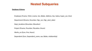
branch (branch_name, branch_city,assets)
customer (customer_name, customer_street, customer_city)
account (account_number, branch_name, balance)
loan (loan_number, branch_name, amount)
depositor (customer_name, account_number)
borrower(customer_name, loan_number)
Find all customers who have an account at all branches located in
Brooklyn.
select distinct S.customer_name
from depositor as S
where not exists (
(select branch_name
from branch
where branch_city = ‘Brooklyn’)
except
(select R.branch_name
from depositor as T, account as R
where T.account_number = R.account_number and
S.customer_name = T.customer_name ))
Note that X – Y = Ø X Y
Note: Cannot write this query using = all and its variants
84.
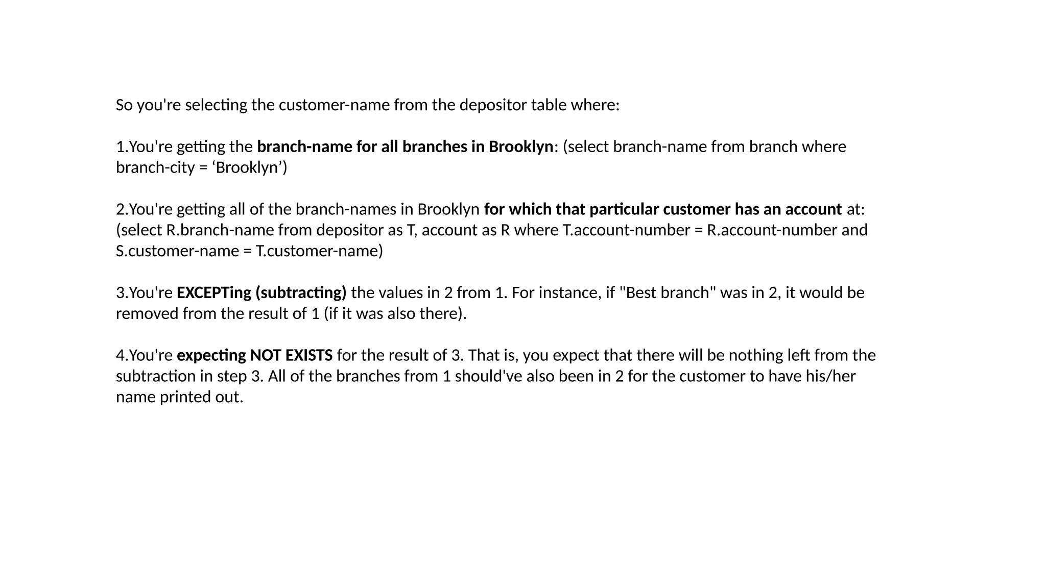
So you're selectingthe customer-name from the depositor table where:
1.You're getting the branch-name for all branches in Brooklyn: (select branch-name from branch where
branch-city = ‘Brooklyn’)
2.You're getting all of the branch-names in Brooklyn for which that particular customer has an account at:
(select R.branch-name from depositor as T, account as R where T.account-number = R.account-number and
S.customer-name = T.customer-name)
3.You're EXCEPTing (subtracting) the values in 2 from 1. For instance, if "Best branch" was in 2, it would be
removed from the result of 1 (if it was also there).
4.You're expecting NOT EXISTS for the result of 3. That is, you expect that there will be nothing left from the
subtraction in step 3. All of the branches from 1 should've also been in 2 for the customer to have his/her
name printed out.
85.
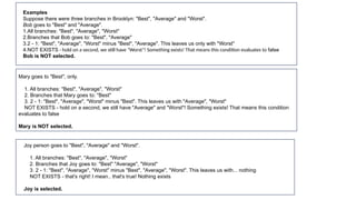
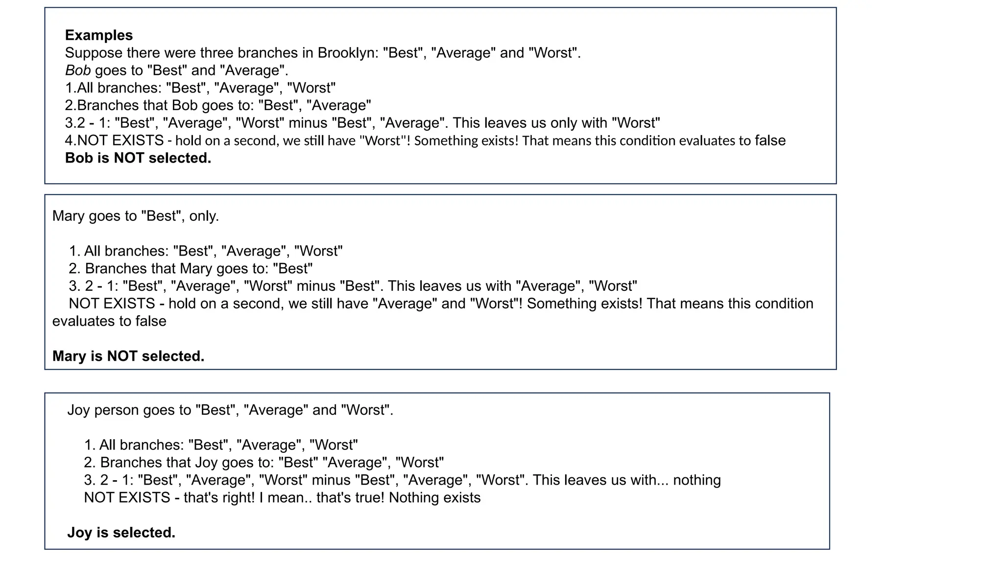
Mary goes to"Best", only.
1. All branches: "Best", "Average", "Worst"
2. Branches that Mary goes to: "Best"
3. 2 - 1: "Best", "Average", "Worst" minus "Best". This leaves us with "Average", "Worst"
NOT EXISTS - hold on a second, we still have "Average" and "Worst"! Something exists! That means this condition
evaluates to false
Mary is NOT selected.
Joy person goes to "Best", "Average" and "Worst".
1. All branches: "Best", "Average", "Worst"
2. Branches that Joy goes to: "Best" "Average", "Worst"
3. 2 - 1: "Best", "Average", "Worst" minus "Best", "Average", "Worst". This leaves us with... nothing
NOT EXISTS - that's right! I mean.. that's true! Nothing exists
Joy is selected.
Examples
Suppose there were three branches in Brooklyn: "Best", "Average" and "Worst".
Bob goes to "Best" and "Average".
1.All branches: "Best", "Average", "Worst"
2.Branches that Bob goes to: "Best", "Average"
3.2 - 1: "Best", "Average", "Worst" minus "Best", "Average". This leaves us only with "Worst"
4.NOT EXISTS - hold on a second, we still have "Worst"! Something exists! That means this condition evaluates to false
Bob is NOT selected.
86.
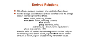
Derived Relations
SQLallows a subquery expression to be used in the from clause
Find the average account balance of those branches where the average
account balance is greater than $1200.
select branch_name, avg_balance
from (select branch_name, avg (balance)
from account
group by branch_name )
as branch_avg ( branch_name, avg_balance )
where avg_balance > 1200
Note that we do not need to use the having clause, since we compute
the temporary (view) relation branch_avg in the from clause, and the
attributes of branch_avg can be used directly in the where clause.
87.
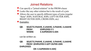
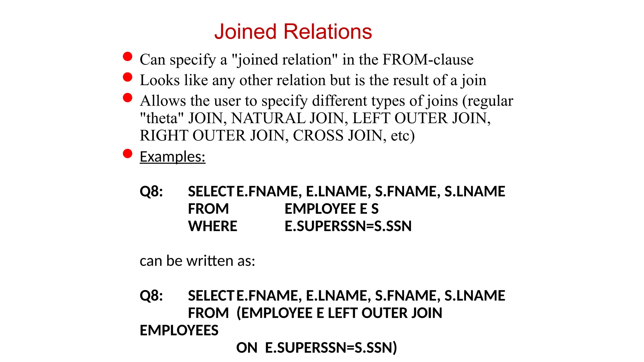
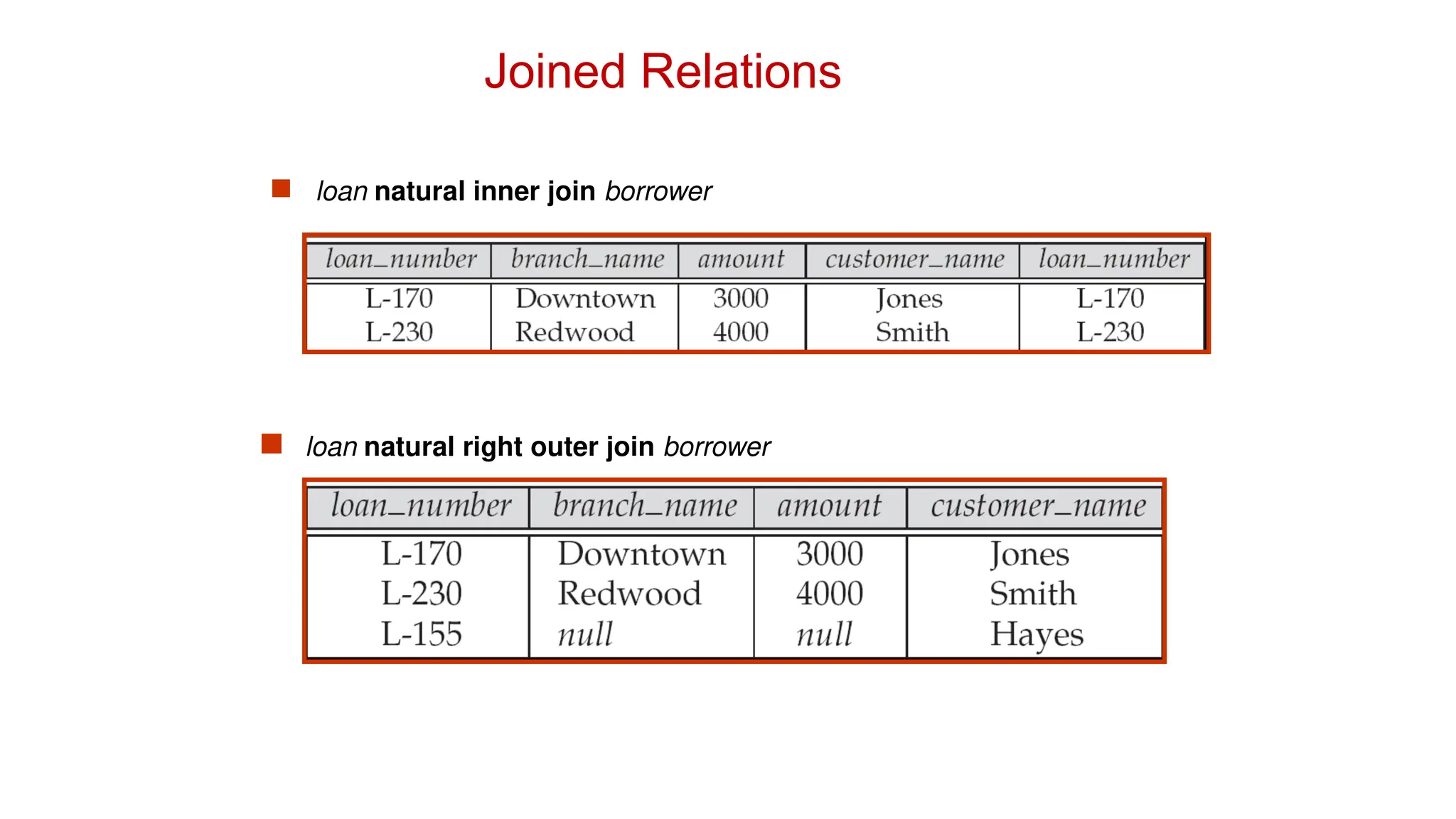
Joined Relations
Can specifya "joined relation" in the FROM-clause
Looks like any other relation but is the result of a join
Allows the user to specify different types of joins (regular
"theta" JOIN, NATURAL JOIN, LEFT OUTER JOIN,
RIGHT OUTER JOIN, CROSS JOIN, etc)
Examples:
Q8: SELECTE.FNAME, E.LNAME, S.FNAME, S.LNAME
FROM EMPLOYEE E S
WHERE E.SUPERSSN=S.SSN
can be written as:
Q8: SELECTE.FNAME, E.LNAME, S.FNAME, S.LNAME
FROM (EMPLOYEE E LEFT OUTER JOIN
EMPLOYEES
ON E.SUPERSSN=S.SSN)
88.
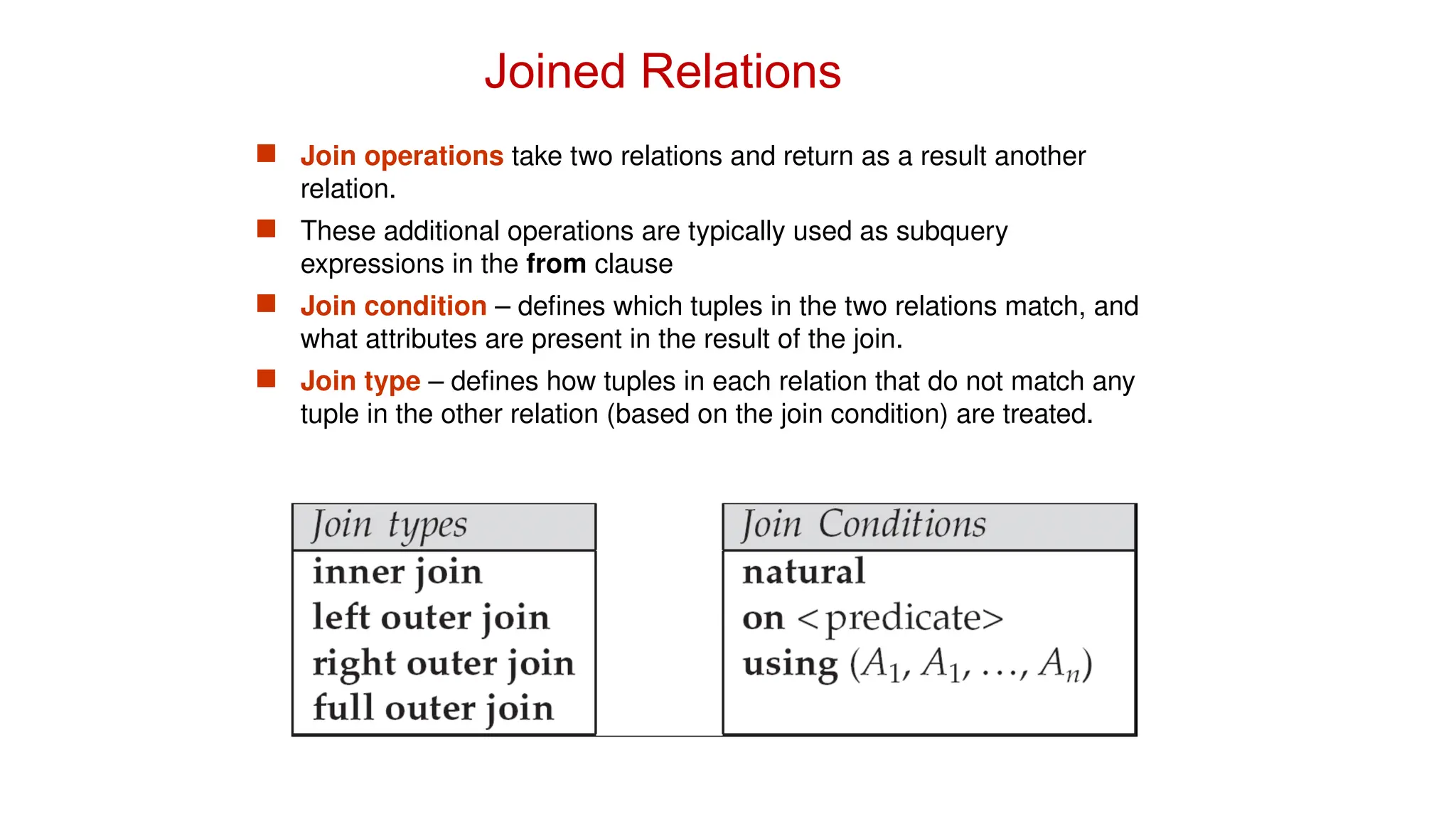
Joined Relations
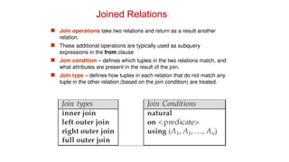
Joinoperations take two relations and return as a result another
relation.
These additional operations are typically used as subquery
expressions in the from clause
Join condition – defines which tuples in the two relations match, and
what attributes are present in the result of the join.
Join type – defines how tuples in each relation that do not match any
tuple in the other relation (based on the join condition) are treated.
89.
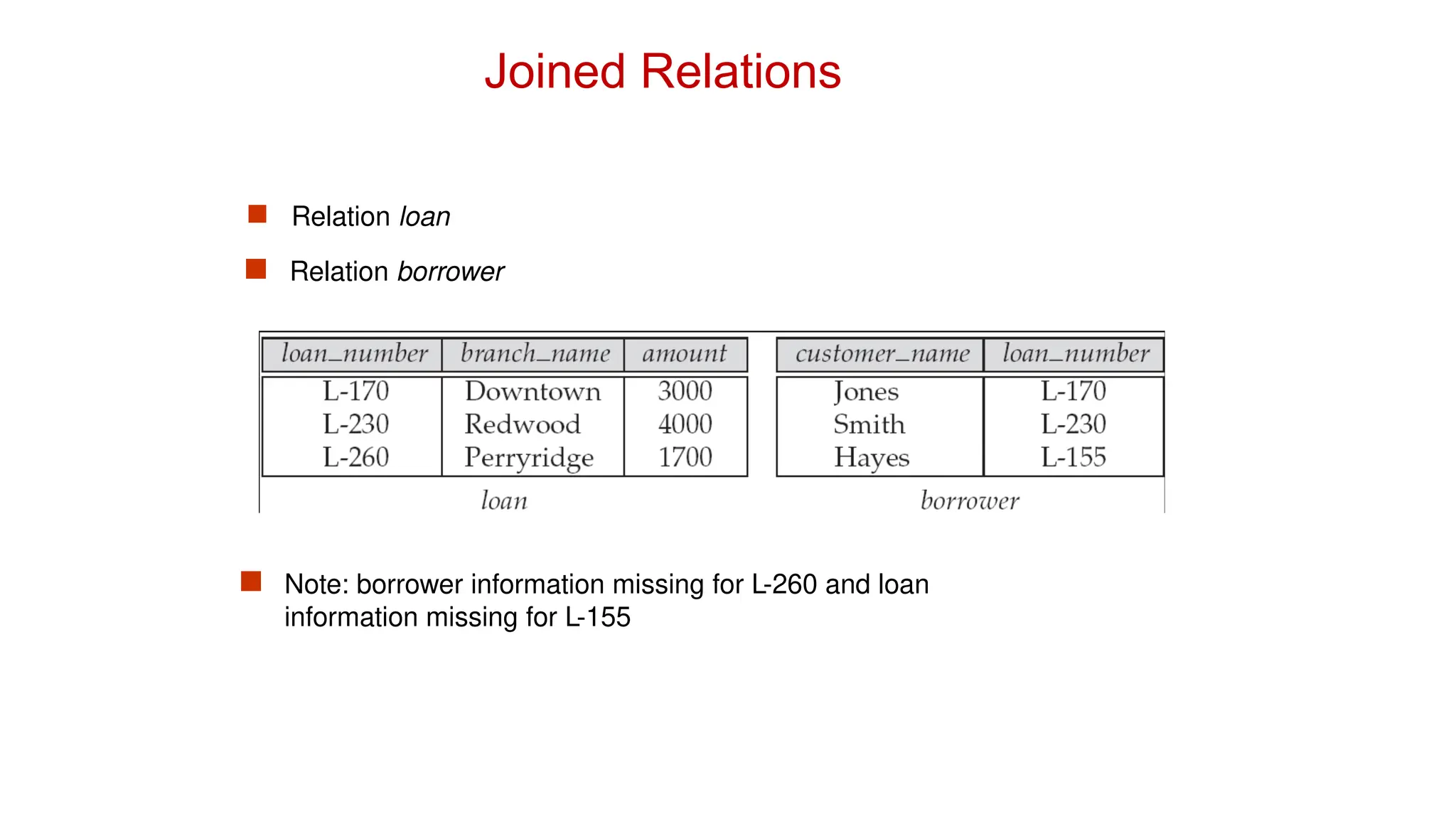
Relation loan
Relation borrower
Note: borrower information missing for L-260 and loan
information missing for L-155
Joined Relations
90.
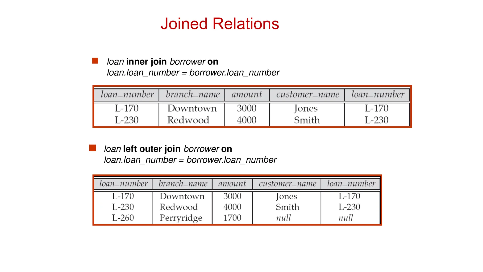
Joined Relations
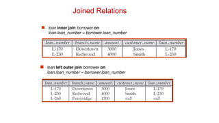
loaninner join borrower on
loan.loan_number = borrower.loan_number
loan left outer join borrower on
loan.loan_number = borrower.loan_number
Joined Relations
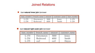
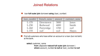
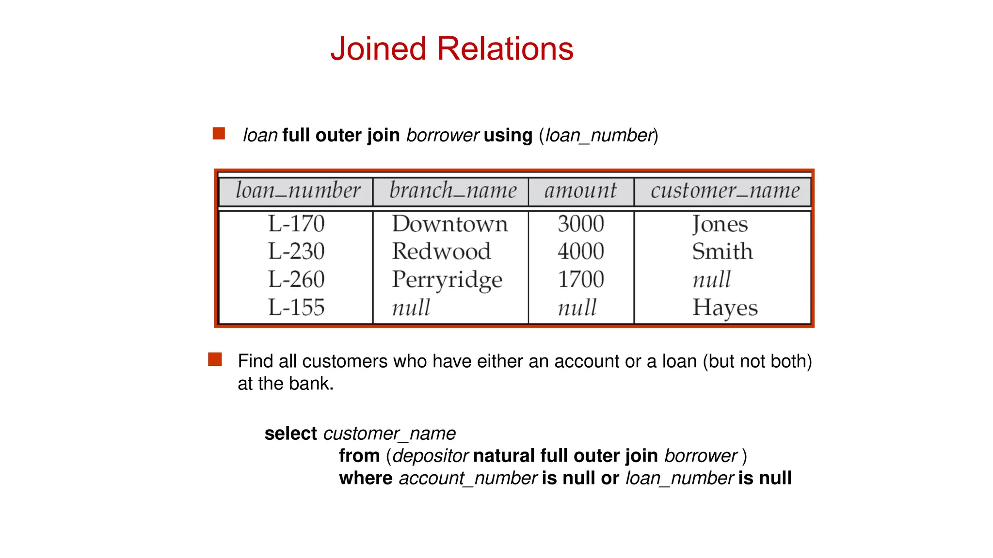
loanfull outer join borrower using (loan_number)
Find all customers who have either an account or a loan (but not both)
at the bank.
select customer_name
from (depositor natural full outer join borrower )
where account_number is null or loan_number is null
93.
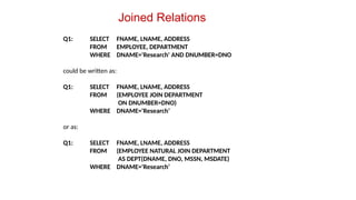
Joined Relations
Q1: SELECTFNAME, LNAME, ADDRESS
FROM EMPLOYEE, DEPARTMENT
WHERE DNAME='Research' AND DNUMBER=DNO
could be written as:
Q1: SELECT FNAME, LNAME, ADDRESS
FROM (EMPLOYEE JOIN DEPARTMENT
ON DNUMBER=DNO)
WHERE DNAME='Research’
or as:
Q1: SELECT FNAME, LNAME, ADDRESS
FROM (EMPLOYEE NATURAL JOIN DEPARTMENT
AS DEPT(DNAME, DNO, MSSN, MSDATE)
WHERE DNAME='Research’
94.
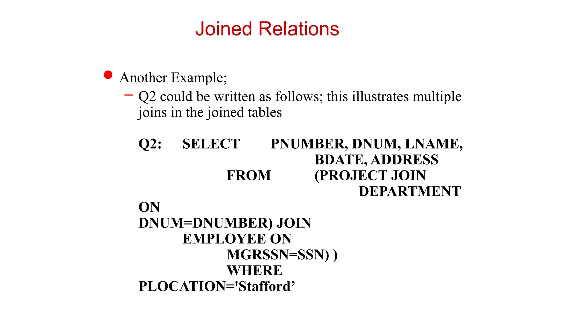
Joined Relations
Another Example;
–Q2 could be written as follows; this illustrates multiple
joins in the joined tables
Q2: SELECT PNUMBER, DNUM, LNAME,
BDATE, ADDRESS
FROM (PROJECT JOIN
DEPARTMENT
ON
DNUM=DNUMBER) JOIN
EMPLOYEE ON
MGRSSN=SSN) )
WHERE
PLOCATION='Stafford’
95.
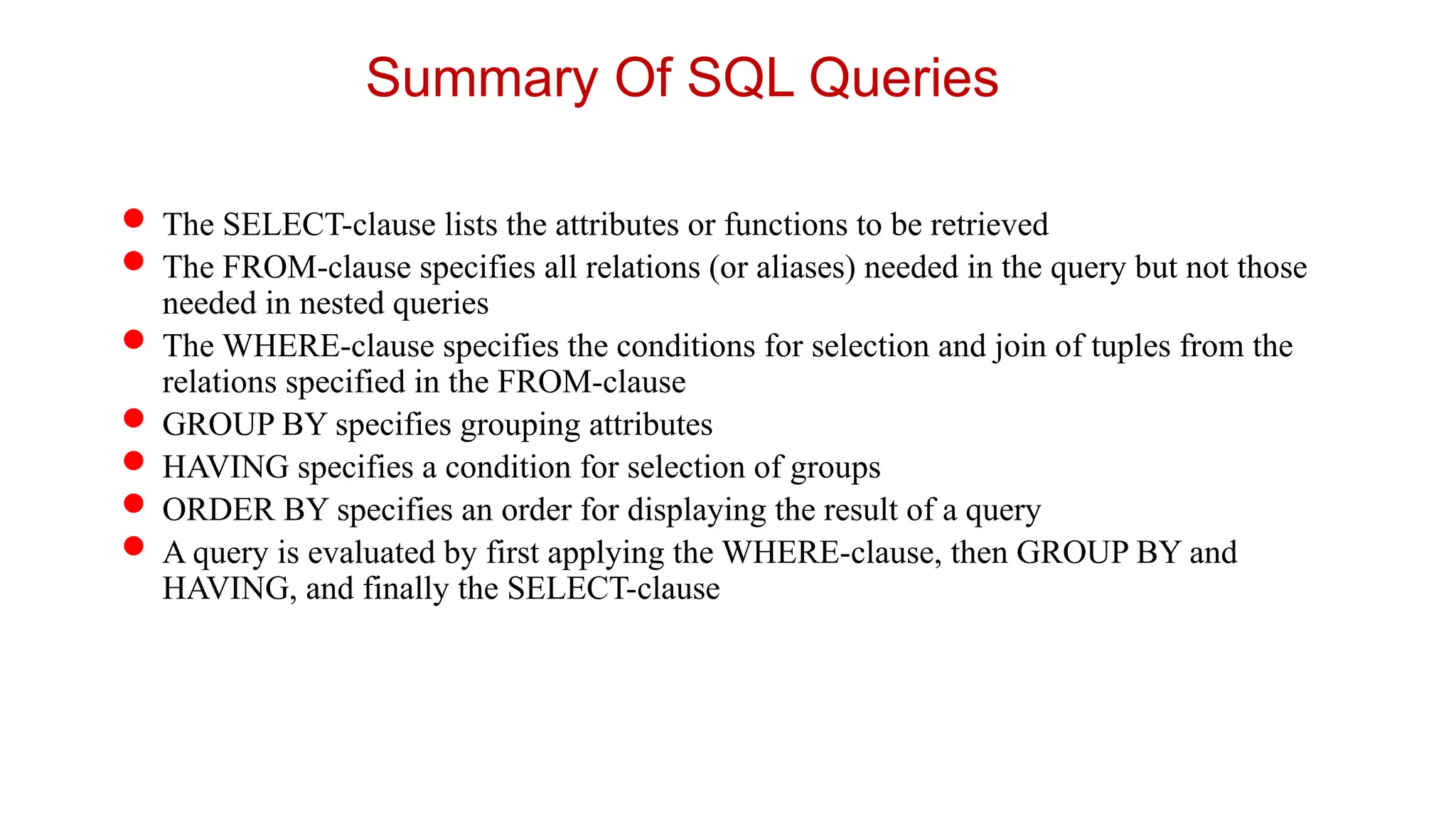
Summary Of SQLQueries
A query in SQL can consist of up to six clauses, but only
the first two, SELECT and FROM, are mandatory. The
clauses are specified in the following order:
SELECT <attribute list>
FROM <table list>
[WHERE <condition>]
[GROUP BY <grouping attribute(s)>]
[HAVING <group condition>]
[ORDER BY <attribute list>]
96.
Summary Of SQLQueries
The SELECT-clause lists the attributes or functions to be retrieved
The FROM-clause specifies all relations (or aliases) needed in the query but not those
needed in nested queries
The WHERE-clause specifies the conditions for selection and join of tuples from the
relations specified in the FROM-clause
GROUP BY specifies grouping attributes
HAVING specifies a condition for selection of groups
ORDER BY specifies an order for displaying the result of a query
A query is evaluated by first applying the WHERE-clause, then GROUP BY and
HAVING, and finally the SELECT-clause
97.
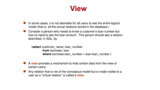
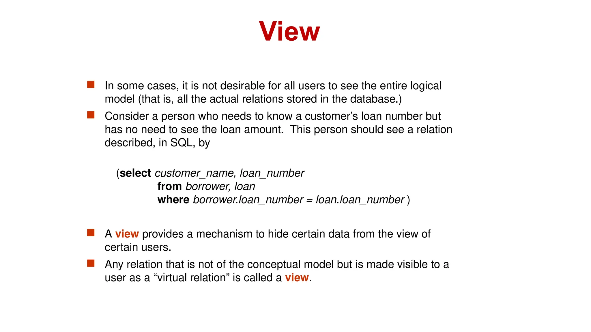
In somecases, it is not desirable for all users to see the entire logical
model (that is, all the actual relations stored in the database.)
Consider a person who needs to know a customer’s loan number but
has no need to see the loan amount. This person should see a relation
described, in SQL, by
(select customer_name, loan_number
from borrower, loan
where borrower.loan_number = loan.loan_number )
A view provides a mechanism to hide certain data from the view of
certain users.
Any relation that is not of the conceptual model but is made visible to a
user as a “virtual relation” is called a view.
View
98.
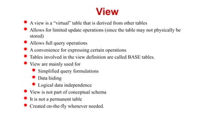
A viewis a “virtual” table that is derived from other tables
Allows for limited update operations (since the table may not physically be
stored)
Allows full query operations
A convenience for expressing certain operations
Tables involved in the view definition are called BASE tables.
View are mainly used for
Simplified query formulations
Data hiding
Logical data independence
View is not part of conceptual schema
It is not a permanent table
Created on-the-fly whenever needed.
View
99.
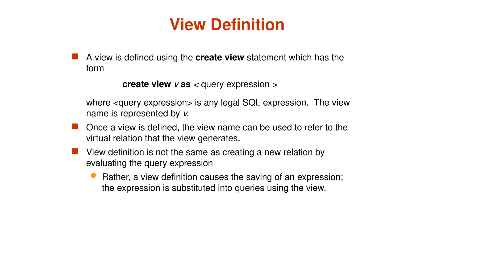
View Definition
Aview is defined using the create view statement which has the
form
create view v as < query expression >
where <query expression> is any legal SQL expression. The view
name is represented by v.
Once a view is defined, the view name can be used to refer to the
virtual relation that the view generates.
View definition is not the same as creating a new relation by
evaluating the query expression
Rather, a view definition causes the saving of an expression;
the expression is substituted into queries using the view.
100.
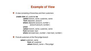
Example of View
A view consisting of branches and their customers
Find all customers of the Perryridge branch
create view all_customer as
(select branch_name, customer_name
from depositor, account
where depositor.account_number =
account.account_number )
union
(select branch_name, customer_name
from borrower, loan
where borrower.loan_number = loan.loan_number )
select customer_name
from all_customer
where branch_name = ‘Perryridge’
101.
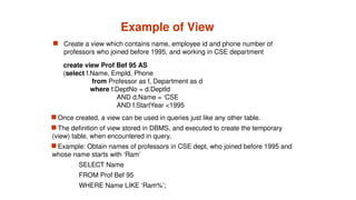
Example of View
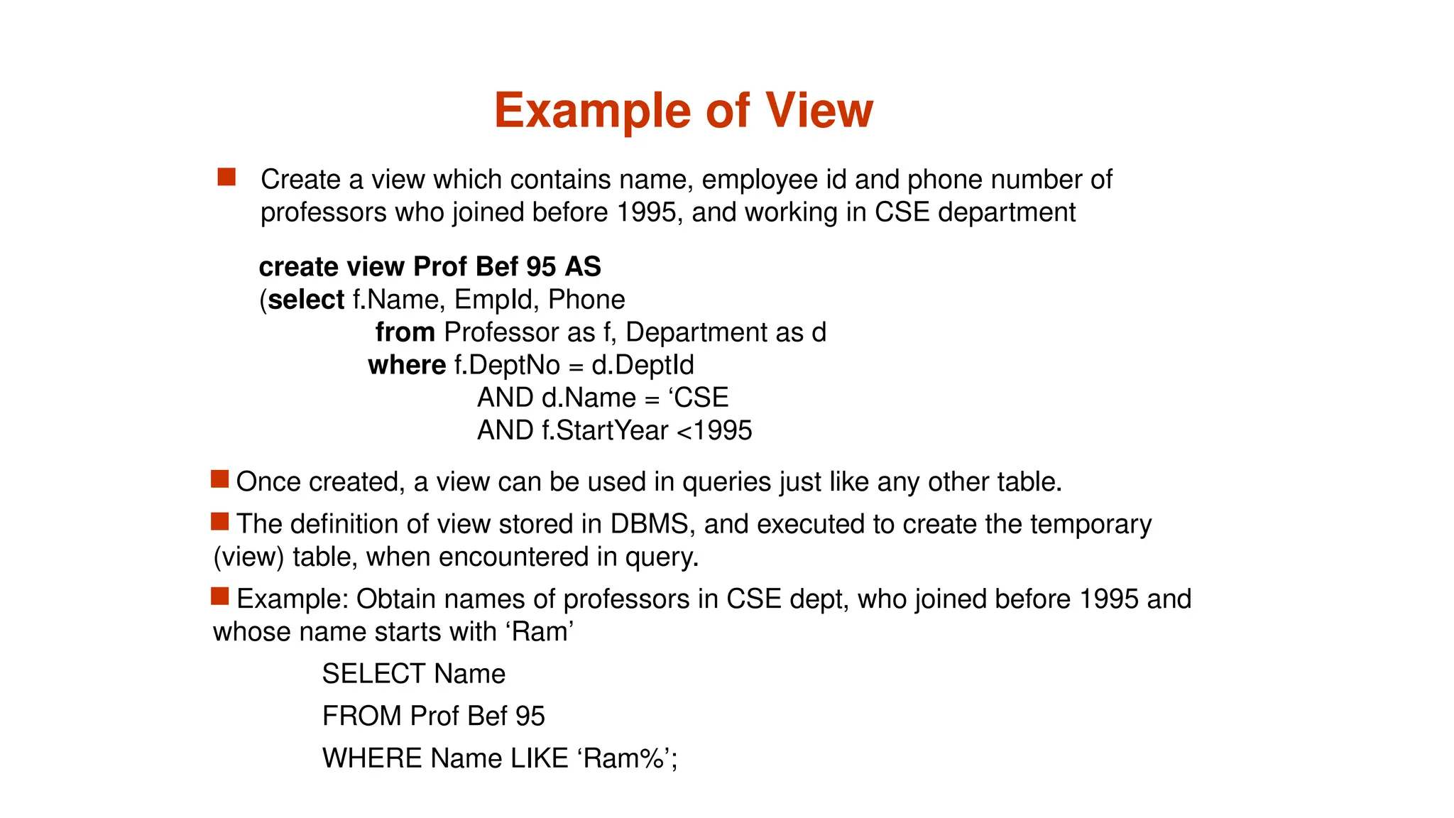
Create a view which contains name, employee id and phone number of
professors who joined before 1995, and working in CSE department
Once created, a view can be used in queries just like any other table.
The definition of view stored in DBMS, and executed to create the temporary
(view) table, when encountered in query.
Example: Obtain names of professors in CSE dept, who joined before 1995 and
whose name starts with ‘Ram’
SELECT Name
FROM Prof Bef 95
WHERE Name LIKE ‘Ram%’;
create view Prof Bef 95 AS
(select f.Name, EmpId, Phone
from Professor as f, Department as d
where f.DeptNo = d.DeptId
AND d.Name = ‘CSE
AND f.StartYear <1995
102.
Operations on View
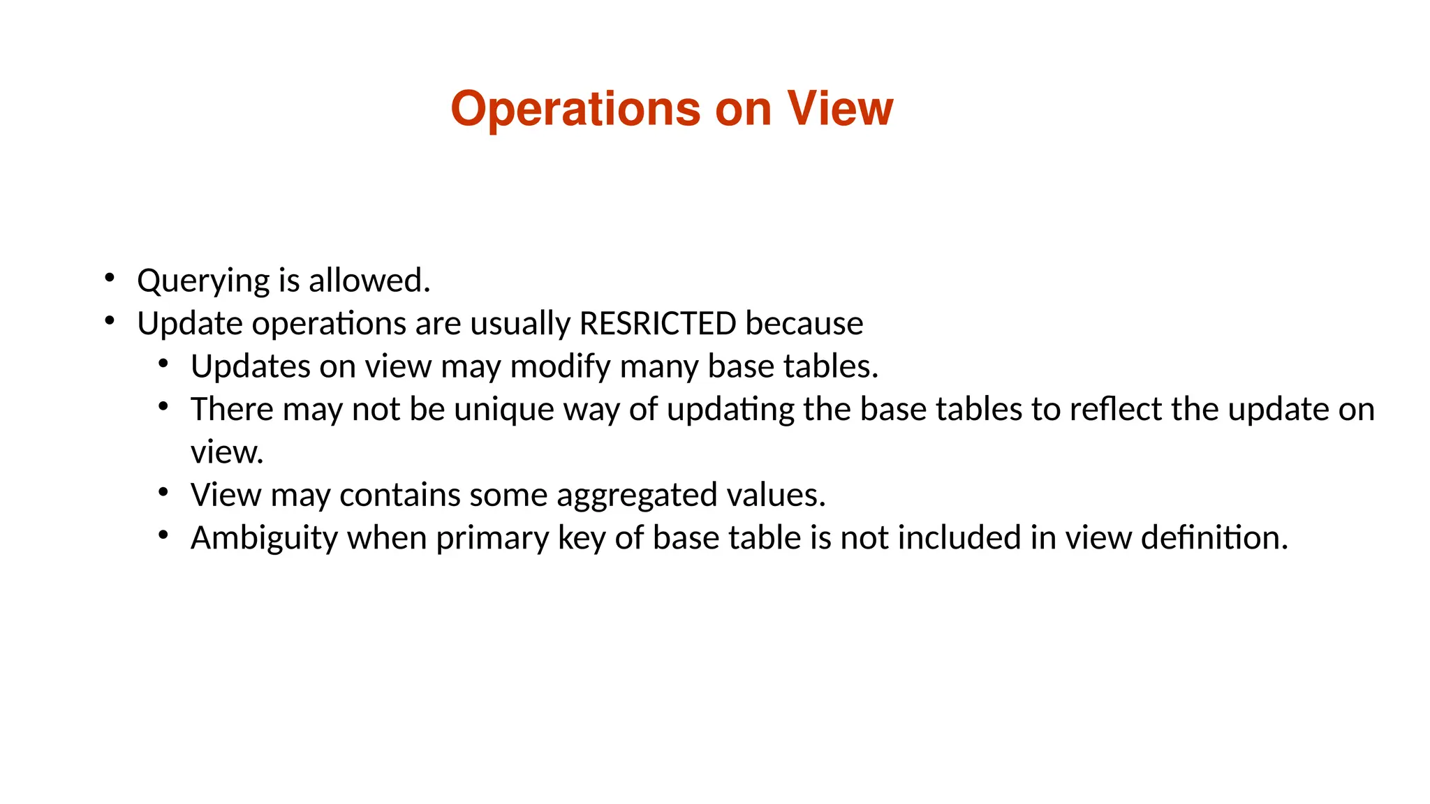
•Querying is allowed.
• Update operations are usually RESRICTED because
• Updates on view may modify many base tables.
• There may not be unique way of updating the base tables to reflect the update on
view.
• View may contains some aggregated values.
• Ambiguity when primary key of base table is not included in view definition.
103.
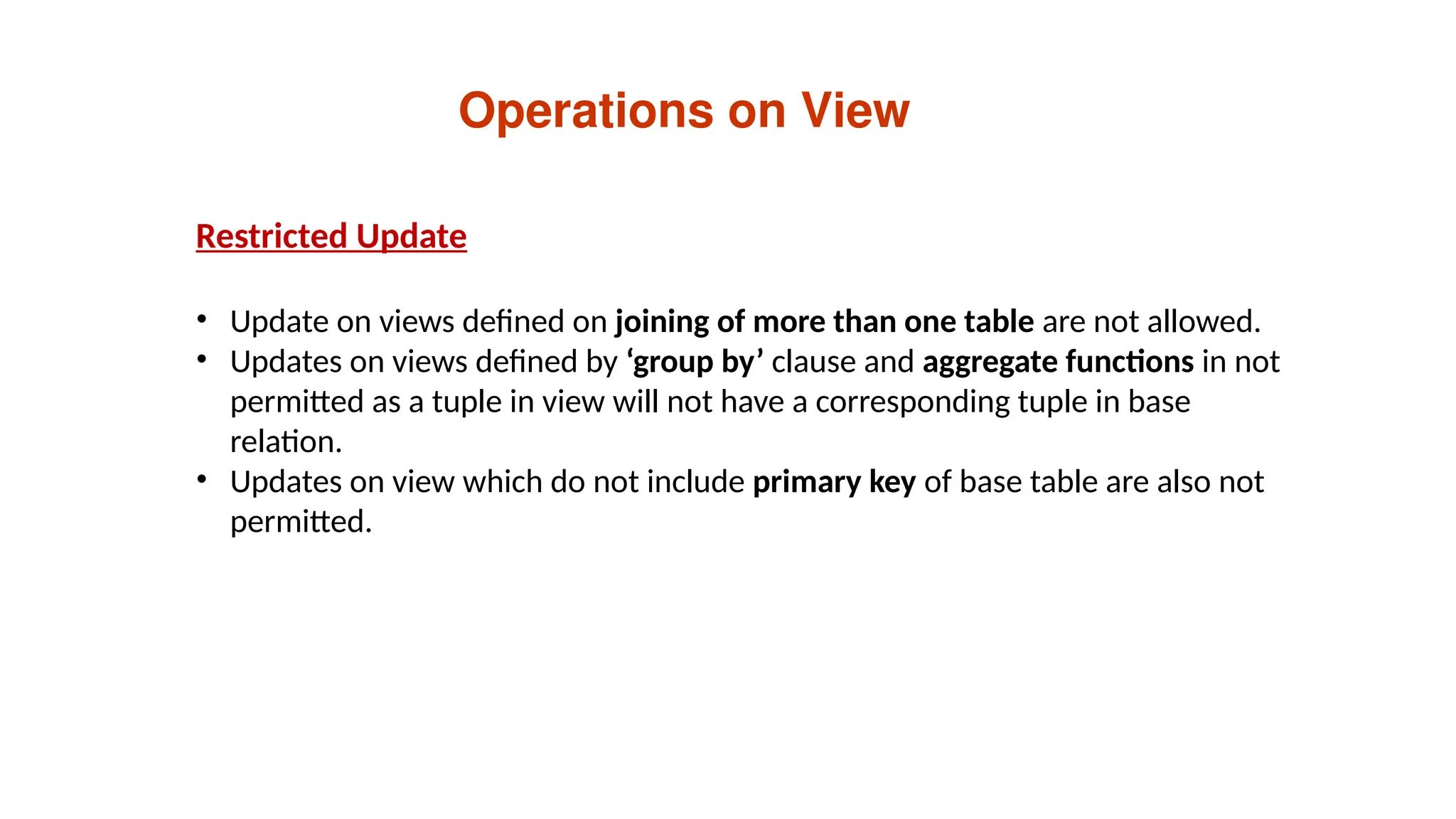
Operations on View
RestrictedUpdate
• Update on views defined on joining of more than one table are not allowed.
• Updates on views defined by ‘group by’ clause and aggregate functions in not
permitted as a tuple in view will not have a corresponding tuple in base
relation.
• Updates on view which do not include primary key of base table are also not
permitted.
104.
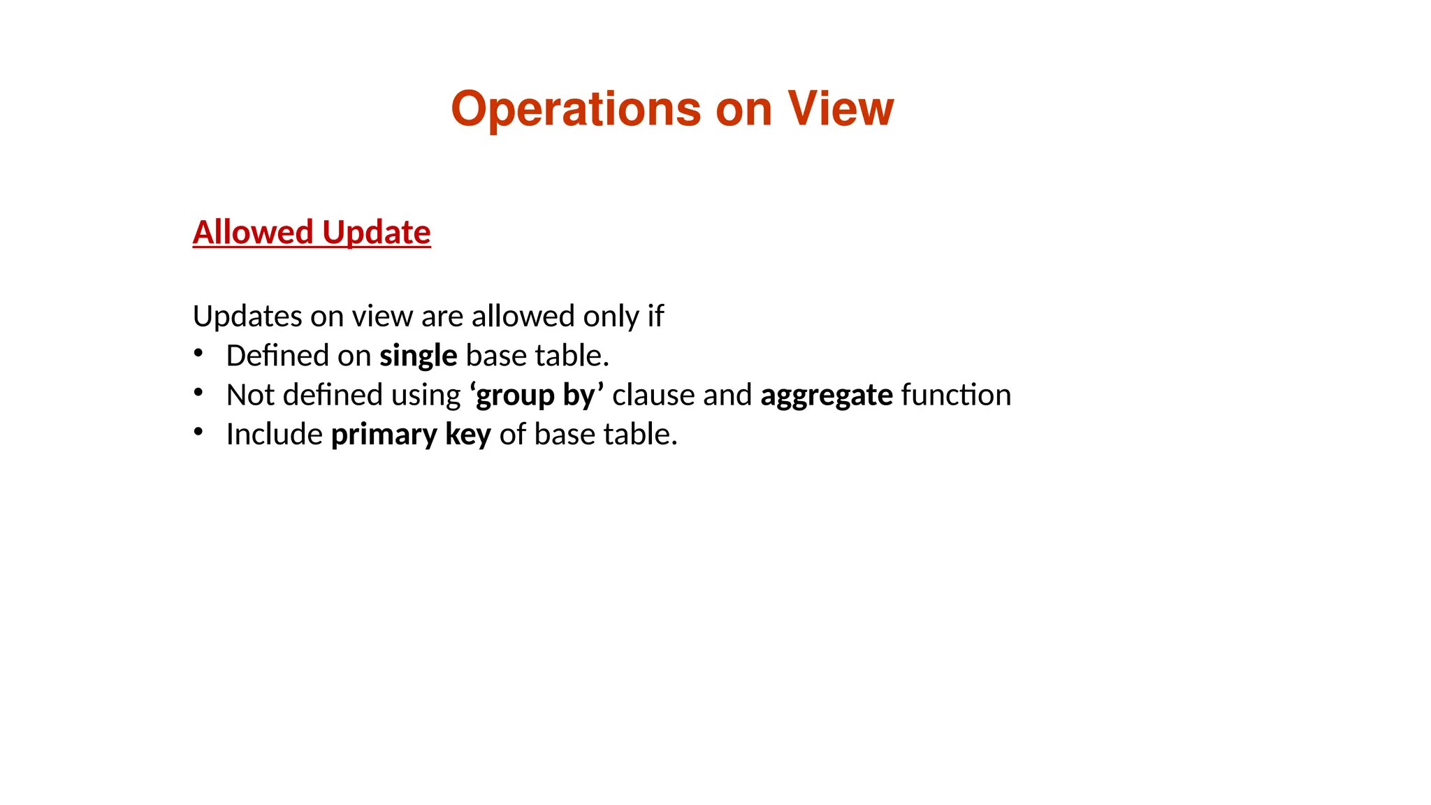
Operations on View
AllowedUpdate
Updates on view are allowed only if
• Defined on single base table.
• Not defined using ‘group by’ clause and aggregate function
• Include primary key of base table.
105.
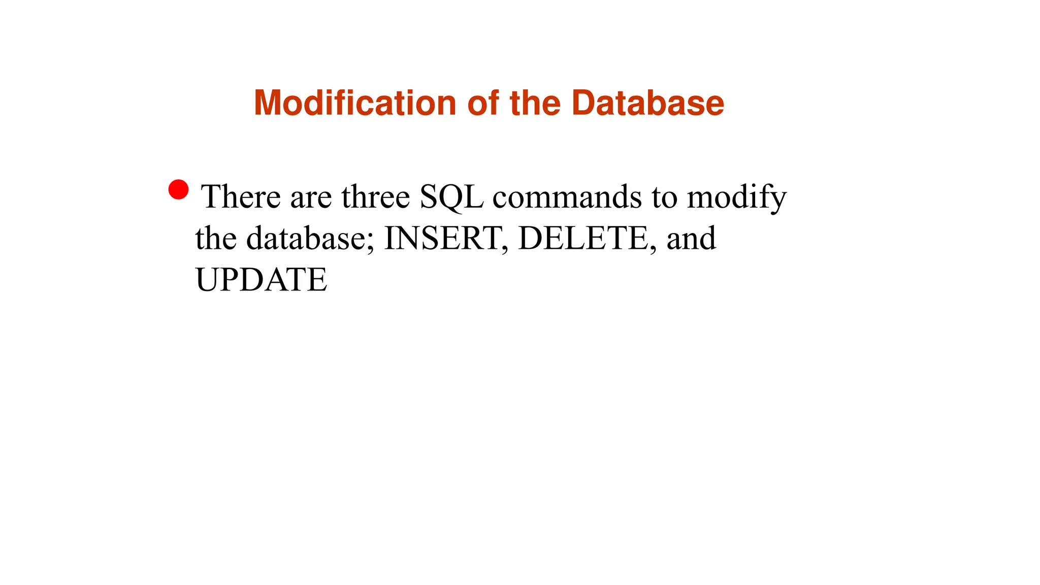
Modification of theDatabase
There are three SQL commands to modify
the database; INSERT, DELETE, and
UPDATE
106.
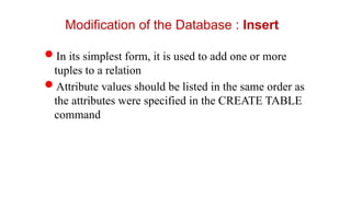
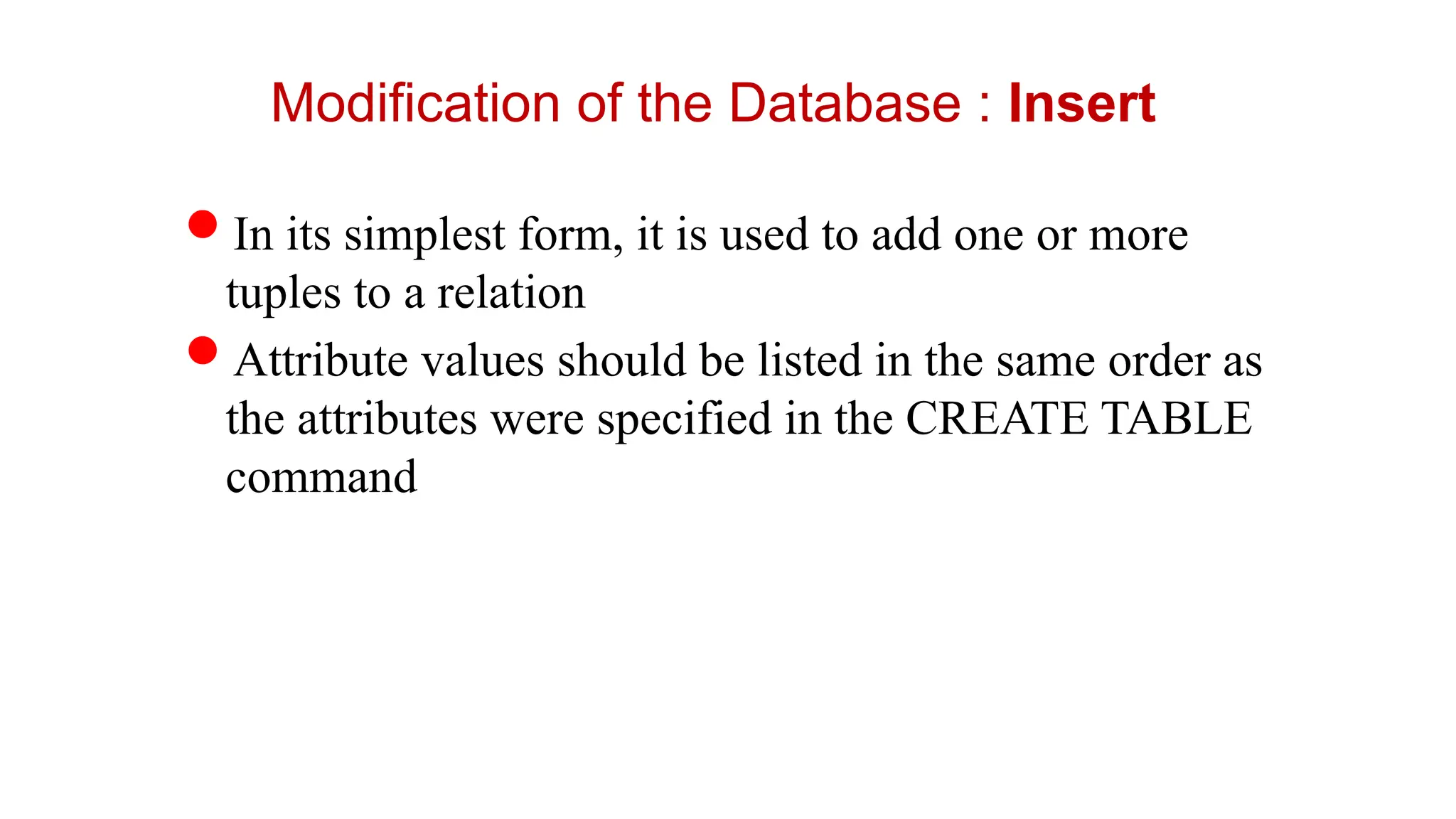
Modification of theDatabase : Insert
In its simplest form, it is used to add one or more
tuples to a relation
Attribute values should be listed in the same order as
the attributes were specified in the CREATE TABLE
command
107.
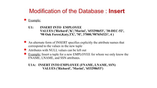
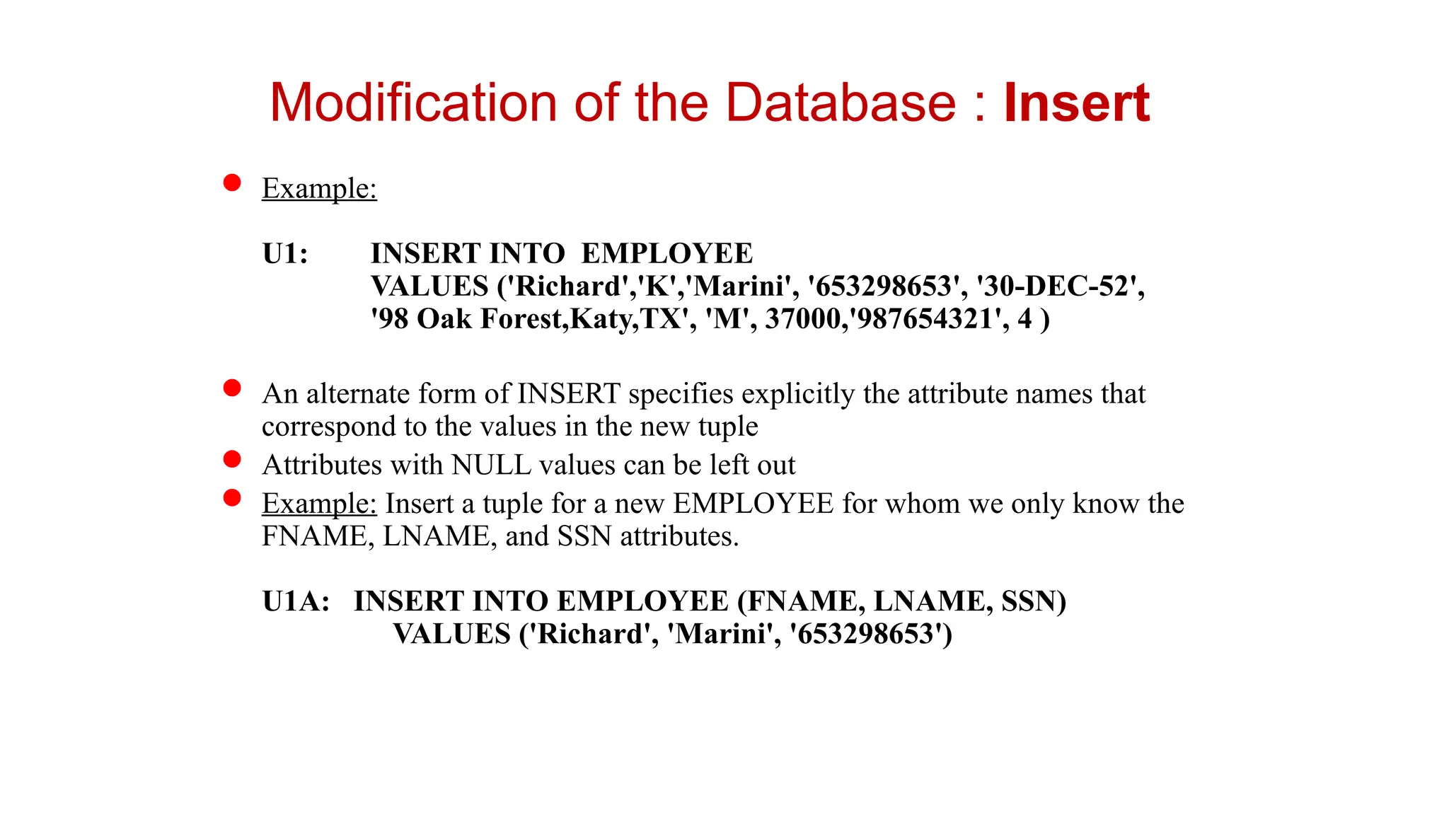
Example:
U1: INSERTINTO EMPLOYEE
VALUES ('Richard','K','Marini', '653298653', '30-DEC-52',
'98 Oak Forest,Katy,TX', 'M', 37000,'987654321', 4 )
An alternate form of INSERT specifies explicitly the attribute names that
correspond to the values in the new tuple
Attributes with NULL values can be left out
Example: Insert a tuple for a new EMPLOYEE for whom we only know the
FNAME, LNAME, and SSN attributes.
U1A: INSERT INTO EMPLOYEE (FNAME, LNAME, SSN)
VALUES ('Richard', 'Marini', '653298653')
Modification of the Database : Insert
108.
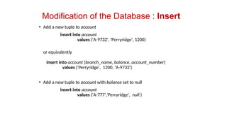
Modification of theDatabase : Insert
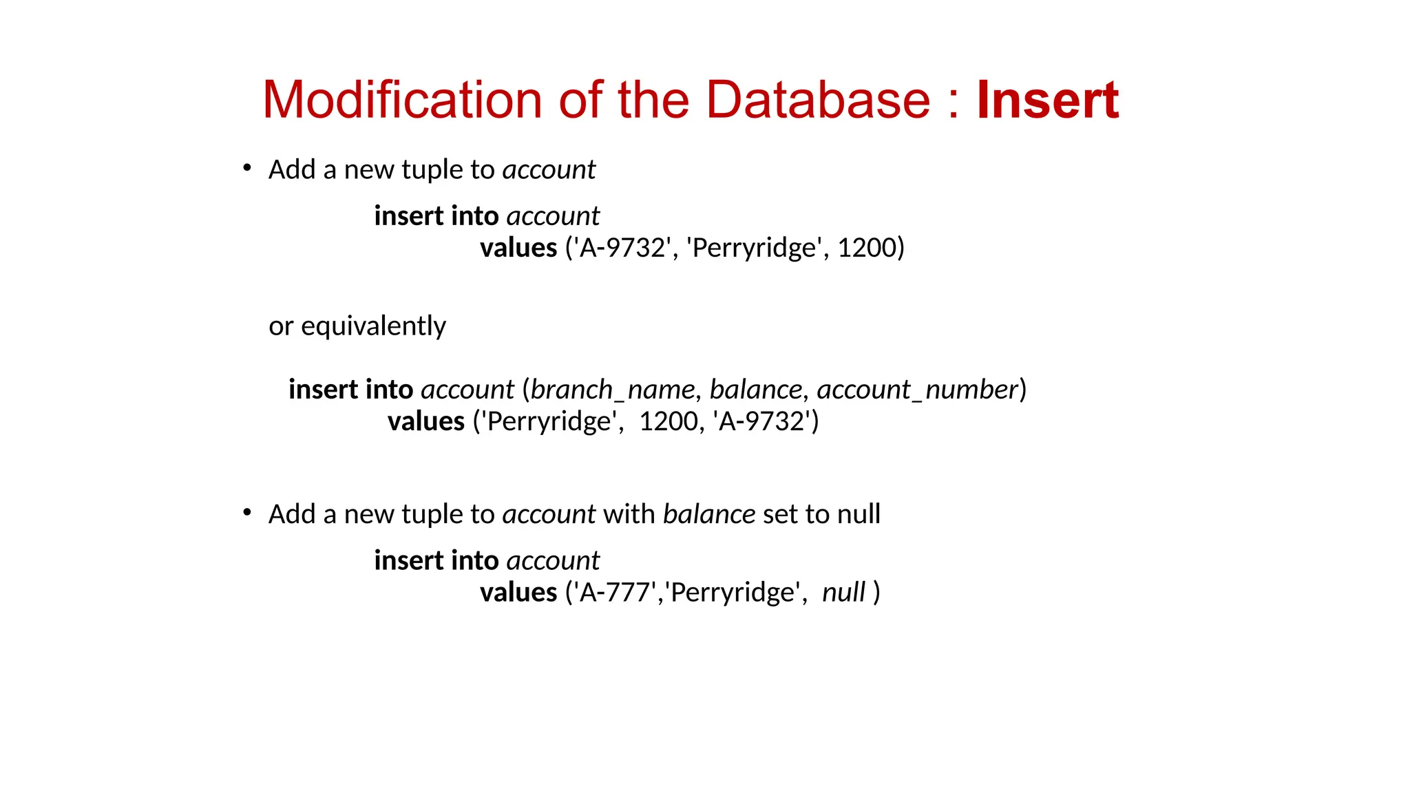
• Add a new tuple to account
insert into account
values ('A-9732', 'Perryridge', 1200)
or equivalently
insert into account (branch_name, balance, account_number)
values ('Perryridge', 1200, 'A-9732')
• Add a new tuple to account with balance set to null
insert into account
values ('A-777','Perryridge', null )
109.
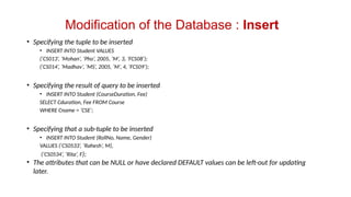
Modification of theDatabase : Insert
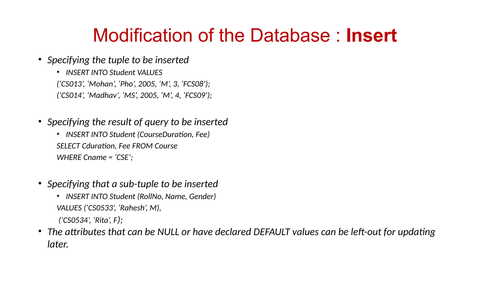
• Specifying the tuple to be inserted
• INSERT INTO Student VALUES
(‘CS013’, ‘Mohan’, ‘Pho’, 2005, ‘M’, 3, ‘FCS08’);
(‘CS014’, ‘Madhav’, ‘MS’, 2005, ‘M’, 4, ‘FCS09’);
• Specifying the result of query to be inserted
• INSERT INTO Student (CourseDuration, Fee)
SELECT Cduration, Fee FROM Course
WHERE Cname = ‘CSE’;
• Specifying that a sub-tuple to be inserted
• INSERT INTO Student (RollNo, Name, Gender)
VALUES (‘CS0533’, ‘Rahesh’, M),
(‘CS0534’, ‘Rita’, F);
• The attributes that can be NULL or have declared DEFAULT values can be left-out for updating
later.
110.
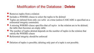
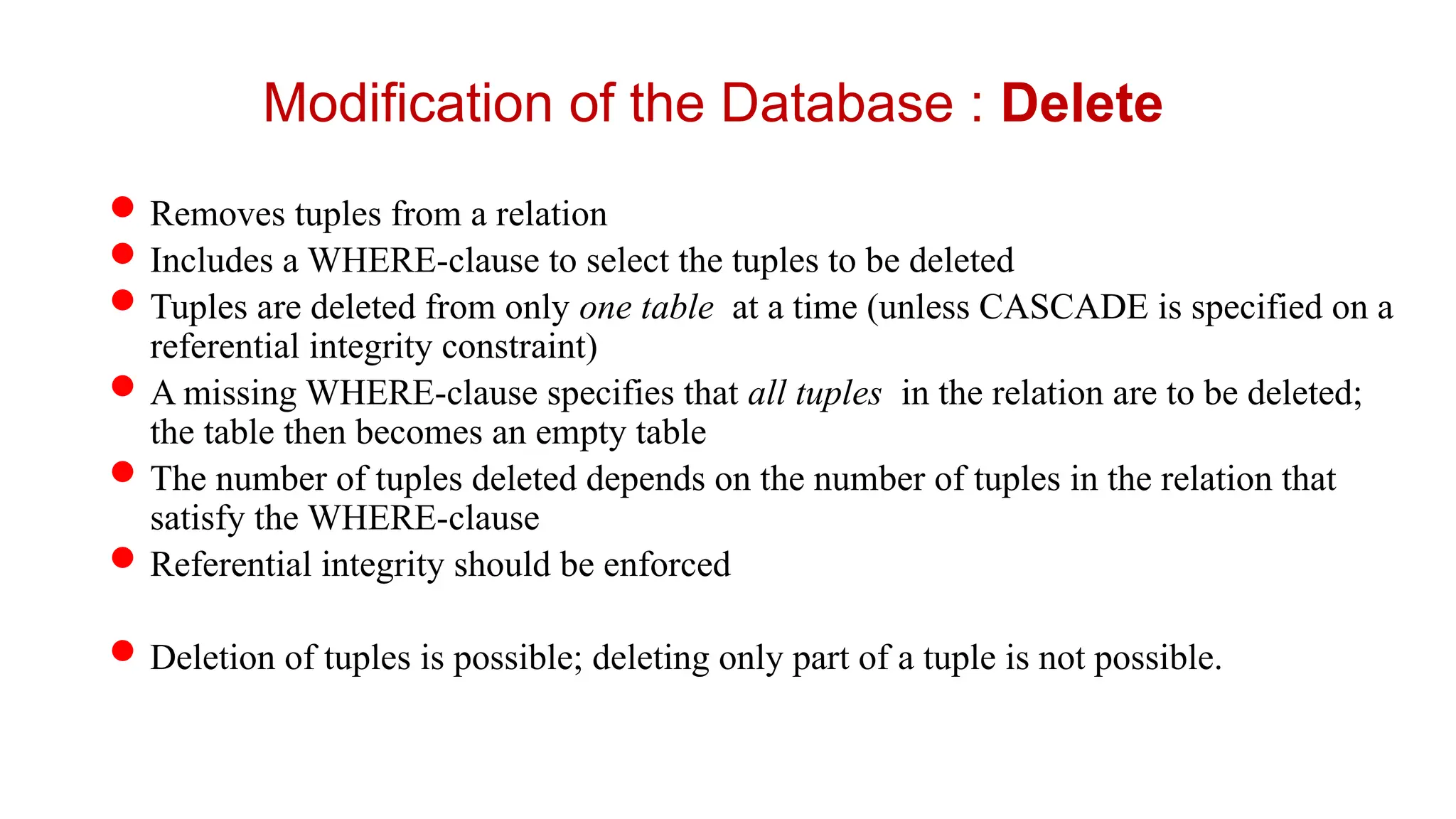
Removes tuples froma relation
Includes a WHERE-clause to select the tuples to be deleted
Tuples are deleted from only one table at a time (unless CASCADE is specified on a
referential integrity constraint)
A missing WHERE-clause specifies that all tuples in the relation are to be deleted;
the table then becomes an empty table
The number of tuples deleted depends on the number of tuples in the relation that
satisfy the WHERE-clause
Referential integrity should be enforced
Deletion of tuples is possible; deleting only part of a tuple is not possible.
Modification of the Database : Delete
111.
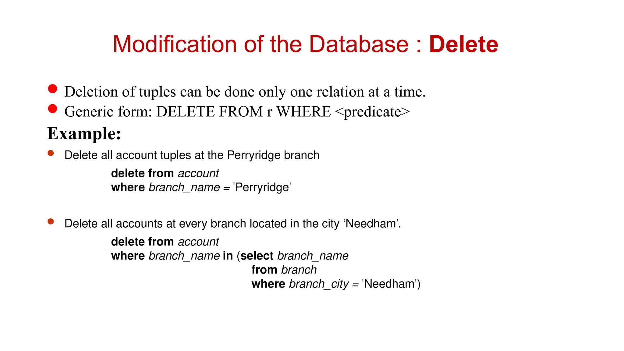
Deletion of tuplescan be done only one relation at a time.
Generic form: DELETE FROM r WHERE <predicate>
Example:
Delete all account tuples at the Perryridge branch
delete from account
where branch_name = 'Perryridge'
Delete all accounts at every branch located in the city ‘Needham’.
delete from account
where branch_name in (select branch_name
from branch
where branch_city = 'Needham')
Modification of the Database : Delete
112.
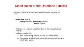
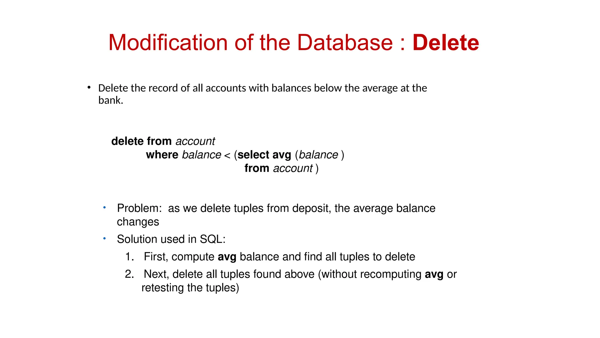
Modification of theDatabase : Delete
• Delete the record of all accounts with balances below the average at the
bank.
delete from account
where balance < (select avg (balance )
from account )
• Problem: as we delete tuples from deposit, the average balance
changes
• Solution used in SQL:
1. First, compute avg balance and find all tuples to delete
2. Next, delete all tuples found above (without recomputing avg or
retesting the tuples)
113.
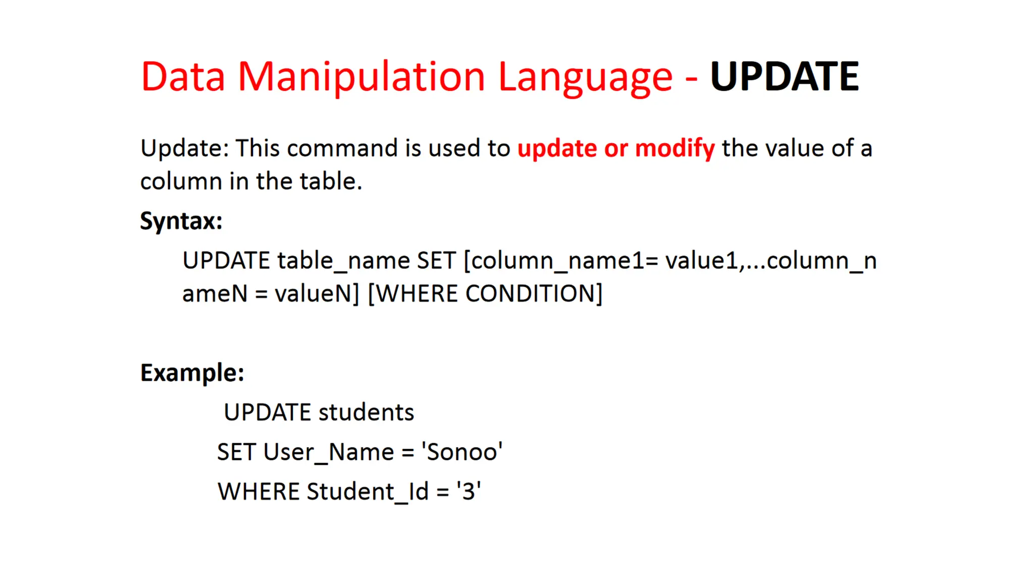
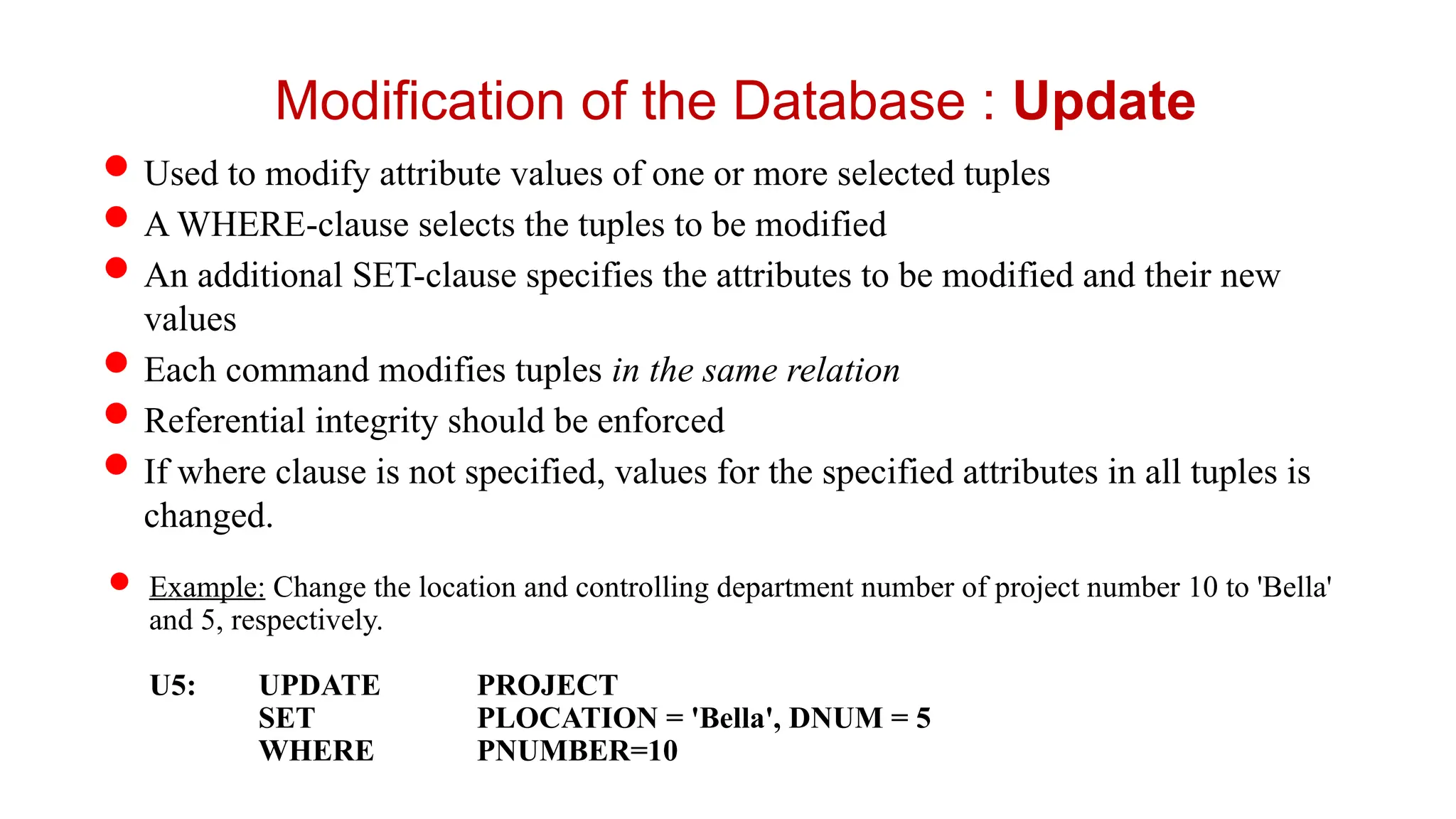
Used to modifyattribute values of one or more selected tuples
A WHERE-clause selects the tuples to be modified
An additional SET-clause specifies the attributes to be modified and their new
values
Each command modifies tuples in the same relation
Referential integrity should be enforced
If where clause is not specified, values for the specified attributes in all tuples is
changed.
Example: Change the location and controlling department number of project number 10 to 'Bella'
and 5, respectively.
U5: UPDATE PROJECT
SET PLOCATION = 'Bella', DNUM = 5
WHERE PNUMBER=10
Modification of the Database : Update
114.
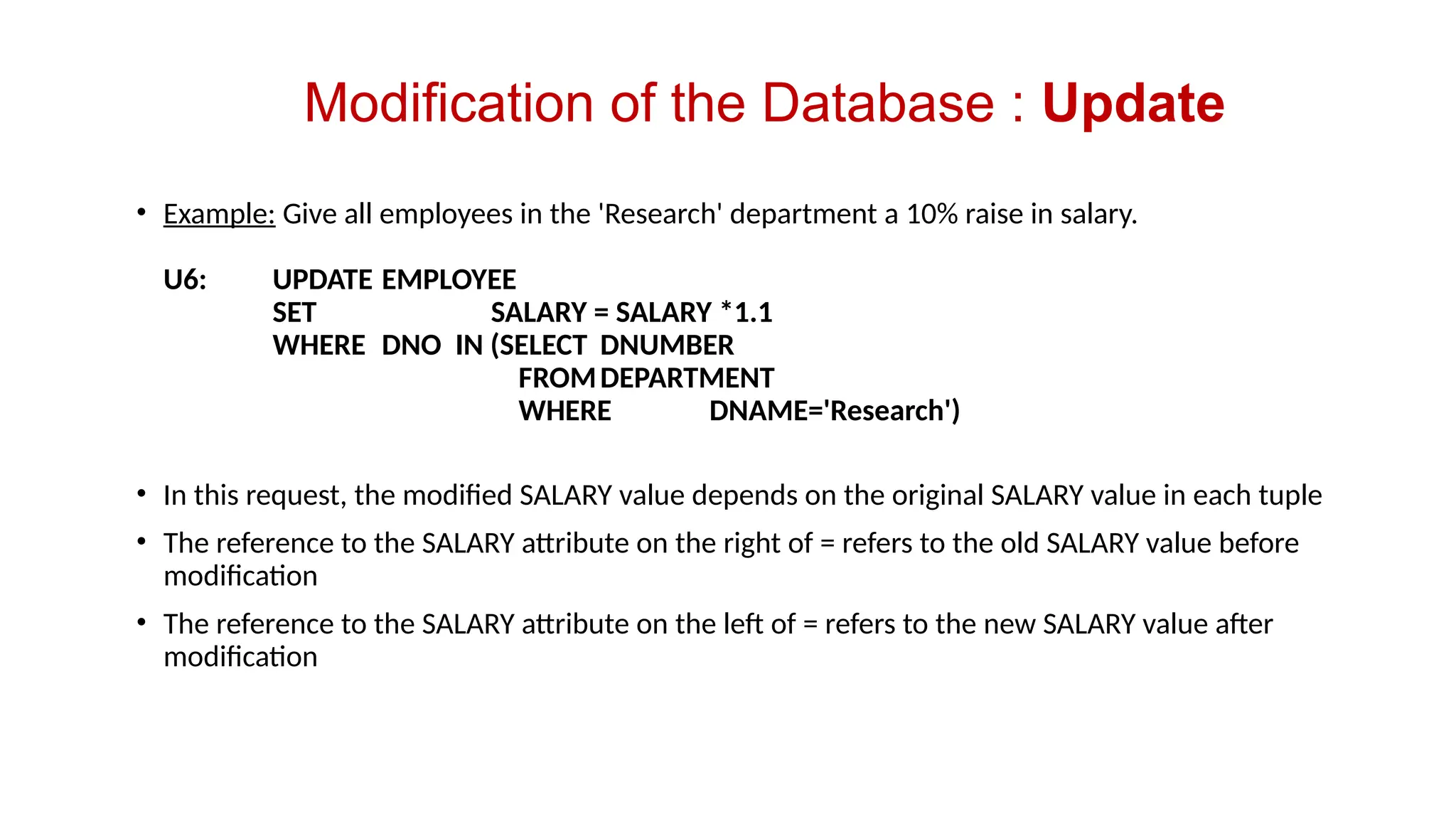
• Example: Giveall employees in the 'Research' department a 10% raise in salary.
U6: UPDATE EMPLOYEE
SET SALARY = SALARY *1.1
WHERE DNO IN (SELECT DNUMBER
FROMDEPARTMENT
WHERE DNAME='Research')
• In this request, the modified SALARY value depends on the original SALARY value in each tuple
• The reference to the SALARY attribute on the right of = refers to the old SALARY value before
modification
• The reference to the SALARY attribute on the left of = refers to the new SALARY value after
modification
Modification of the Database : Update
115.
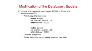
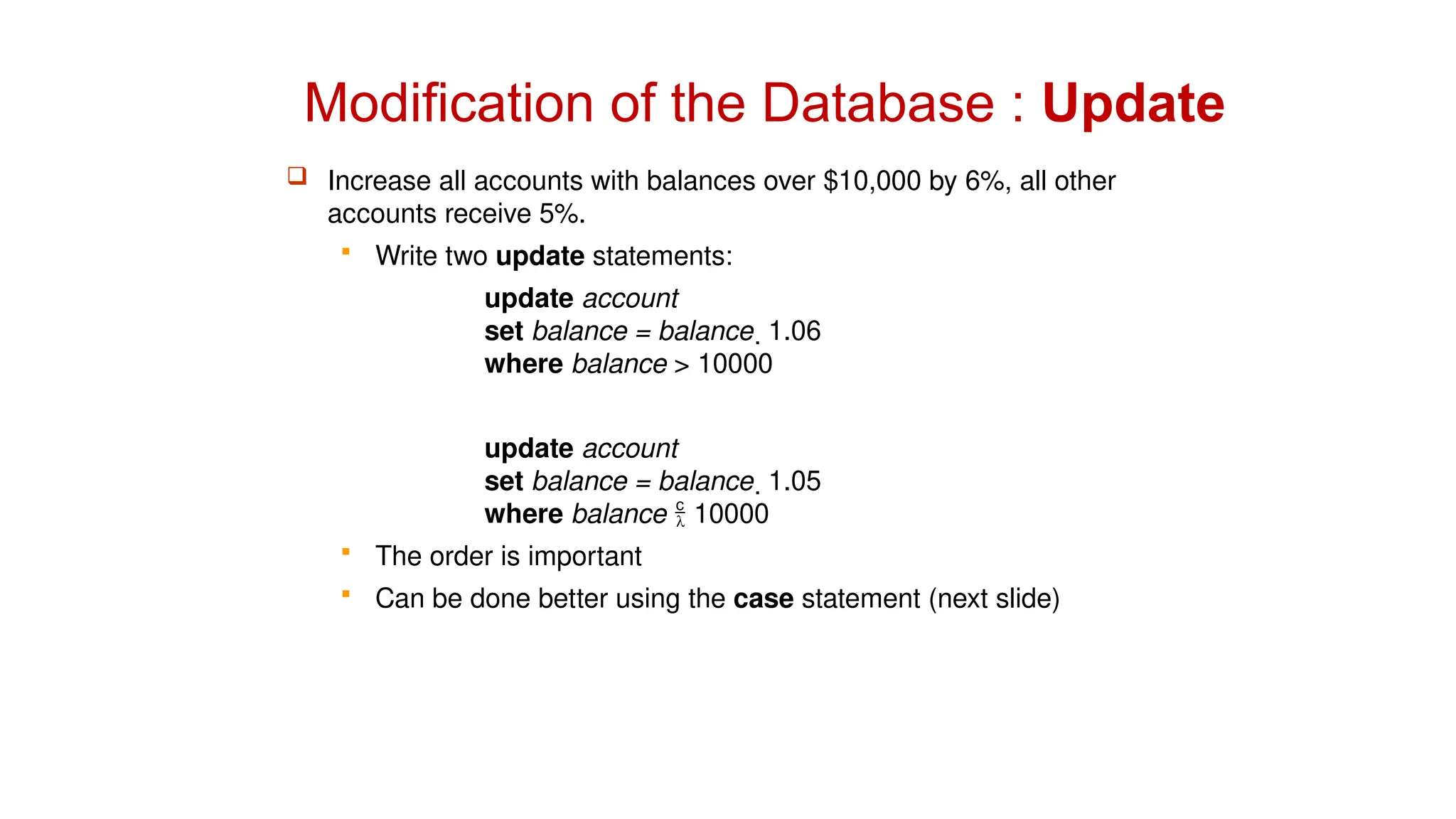
Modification of theDatabase : Update
Increase all accounts with balances over $10,000 by 6%, all other
accounts receive 5%.
Write two update statements:
update account
set balance = balance 1.06
where balance > 10000
update account
set balance = balance 1.05
where balance 10000
The order is important
Can be done better using the case statement (next slide)
116.
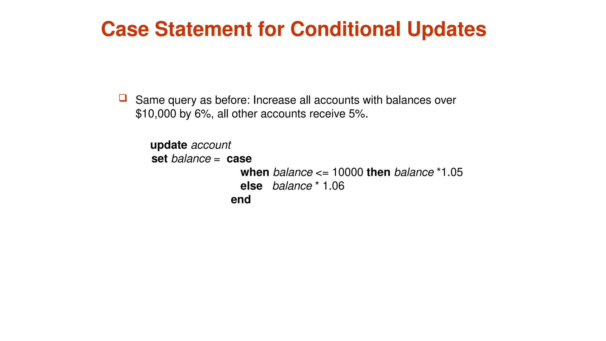
Case Statement forConditional Updates
Same query as before: Increase all accounts with balances over
$10,000 by 6%, all other accounts receive 5%.
update account
set balance = case
when balance <= 10000 then balance *1.05
else balance * 1.06
end


![CREATE TABLE [CUSTOMER]
(
CustomerId int IDENTITY(1,1) PRIMARY KEY,
CustomerNumber int NOT NULL UNIQUE,
LastName varchar(50) NOT NULL,
FirstName varchar(50) NOT NULL,
AreaCode int NULL,
Address varchar(50) NULL,
Phone varchar(50) NULL,
)
SQL Constraints
1. PRIMARY KEY
The PRIMARY KEY constraint uniquely identifies each record in a database table.
Each table should have a primary key, and each table can have only ONE primary key.
Here, IDENTITY(1,1) means the first value will be 1 and then it will increment by 1.](https://image.slidesharecdn.com/part4-250802050931-c1b792f0/85/Presentation-on-SQL-Basics-to-Advance-in-DBMS-11-320.jpg)
![SQL Constraints
3. NOT NULL / Required Columns
The NOT NULL constraint enforces a column to NOT accept NULL values.
The NOT NULL constraint enforces a field to always contain a value.
This means that you cannot insert a new record, or update a record without adding a value to
this field
CREATE TABLE [CUSTOMER]
(
CustomerId int IDENTITY(1,1) PRIMARY KEY,
CustomerNumber int NOT NULL UNIQUE,
LastName varchar(50) NOT NULL,
FirstName varchar(50) NOT NULL,
AreaCode int NULL,
Address varchar(50) NULL,
Phone varchar(50) NULL,
)
Note! A primary key column cannot contain NULL values.](https://image.slidesharecdn.com/part4-250802050931-c1b792f0/85/Presentation-on-SQL-Basics-to-Advance-in-DBMS-15-320.jpg)
![SQL Constraints
4. UNIQUE
The UNIQUE constraint uniquely identifies each record in a database table.
The UNIQUE and PRIMARY KEY constraints both provide a guarantee for uniqueness for a column
or set of columns.
A PRIMARY KEY constraint automatically has a UNIQUE constraint defined on it.
Note! You can have many UNIQUE constraints per table, but only one PRIMARY KEY constraint per
table.
CREATE TABLE [CUSTOMER]
(
CustomerId int IDENTITY(1,1) PRIMARY KEY,
CustomerNumber int NOT NULL UNIQUE,
LastName varchar(50) NOT NULL,
FirstName varchar(50) NOT NULL,
AreaCode int NULL,
Address varchar(50) NULL,
Phone varchar(50) NULL,
)](https://image.slidesharecdn.com/part4-250802050931-c1b792f0/85/Presentation-on-SQL-Basics-to-Advance-in-DBMS-16-320.jpg)
![5. CHECK
The CHECK constraint is used to limit the value range that can be placed in a column.
SQL Constraints
CREATE TABLE [CUSTOMER]
(
CustomerId int IDENTITY(1,1) PRIMARY KEY,
CustomerNumber int NOT NULL UNIQUE CHECK(CustomerNumber>0),
LastName varchar(50) NOT NULL,
FirstName varchar(50) NOT NULL,
AreaCode int NULL,
Address varchar(50) NULL,
Phone varchar(50) NULL,
)](https://image.slidesharecdn.com/part4-250802050931-c1b792f0/85/Presentation-on-SQL-Basics-to-Advance-in-DBMS-17-320.jpg)
![6. DEFAULT
The DEFAULT constraint is used to insert a default value into a column.
The default value will be added to all new records, if no other value is specified..
SQL Constraints
CREATE TABLE [CUSTOMER]
(
CustomerId int IDENTITY(1,1) PRIMARY KEY,
CustomerNumber int NOT NULL UNIQUE,
LastName varchar(50) NOT NULL,
FirstName varchar(50) NOT NULL,
Country varchar(20) DEFAULT 'Norway',
AreaCode int NULL,
Address varchar(50) NULL,
Phone varchar(50) NULL,
)](https://image.slidesharecdn.com/part4-250802050931-c1b792f0/85/Presentation-on-SQL-Basics-to-Advance-in-DBMS-18-320.jpg)


![Summary Of SQL Queries
A query in SQL can consist of up to six clauses, but only
the first two, SELECT and FROM, are mandatory. The
clauses are specified in the following order:
SELECT <attribute list>
FROM <table list>
[WHERE <condition>]
[GROUP BY <grouping attribute(s)>]
[HAVING <group condition>]
[ORDER BY <attribute list>]](https://image.slidesharecdn.com/part4-250802050931-c1b792f0/85/Presentation-on-SQL-Basics-to-Advance-in-DBMS-95-320.jpg)


![CREATE TABLE [CUSTOMER]
(
CustomerId int IDENTITY(1,1) PRIMARY KEY,
CustomerNumber int NOT NULL UNIQUE,
LastName varchar(50) NOT NULL,
FirstName varchar(50) NOT NULL,
AreaCode int NULL,
Address varchar(50) NULL,
Phone varchar(50) NULL,
)
SQL Constraints
1. PRIMARY KEY
The PRIMARY KEY constraint uniquely identifies each record in a database table.
Each table should have a primary key, and each table can have only ONE primary key.
Here, IDENTITY(1,1) means the first value will be 1 and then it will increment by 1.](https://image.slidesharecdn.com/part4-250802050931-c1b792f0/75/Presentation-on-SQL-Basics-to-Advance-in-DBMS-11-2048.jpg)
![SQL Constraints
3. NOT NULL / Required Columns
The NOT NULL constraint enforces a column to NOT accept NULL values.
The NOT NULL constraint enforces a field to always contain a value.
This means that you cannot insert a new record, or update a record without adding a value to
this field
CREATE TABLE [CUSTOMER]
(
CustomerId int IDENTITY(1,1) PRIMARY KEY,
CustomerNumber int NOT NULL UNIQUE,
LastName varchar(50) NOT NULL,
FirstName varchar(50) NOT NULL,
AreaCode int NULL,
Address varchar(50) NULL,
Phone varchar(50) NULL,
)
Note! A primary key column cannot contain NULL values.](https://image.slidesharecdn.com/part4-250802050931-c1b792f0/75/Presentation-on-SQL-Basics-to-Advance-in-DBMS-15-2048.jpg)
![SQL Constraints
4. UNIQUE
The UNIQUE constraint uniquely identifies each record in a database table.
The UNIQUE and PRIMARY KEY constraints both provide a guarantee for uniqueness for a column
or set of columns.
A PRIMARY KEY constraint automatically has a UNIQUE constraint defined on it.
Note! You can have many UNIQUE constraints per table, but only one PRIMARY KEY constraint per
table.
CREATE TABLE [CUSTOMER]
(
CustomerId int IDENTITY(1,1) PRIMARY KEY,
CustomerNumber int NOT NULL UNIQUE,
LastName varchar(50) NOT NULL,
FirstName varchar(50) NOT NULL,
AreaCode int NULL,
Address varchar(50) NULL,
Phone varchar(50) NULL,
)](https://image.slidesharecdn.com/part4-250802050931-c1b792f0/75/Presentation-on-SQL-Basics-to-Advance-in-DBMS-16-2048.jpg)
![5. CHECK
The CHECK constraint is used to limit the value range that can be placed in a column.
SQL Constraints
CREATE TABLE [CUSTOMER]
(
CustomerId int IDENTITY(1,1) PRIMARY KEY,
CustomerNumber int NOT NULL UNIQUE CHECK(CustomerNumber>0),
LastName varchar(50) NOT NULL,
FirstName varchar(50) NOT NULL,
AreaCode int NULL,
Address varchar(50) NULL,
Phone varchar(50) NULL,
)](https://image.slidesharecdn.com/part4-250802050931-c1b792f0/75/Presentation-on-SQL-Basics-to-Advance-in-DBMS-17-2048.jpg)
![6. DEFAULT
The DEFAULT constraint is used to insert a default value into a column.
The default value will be added to all new records, if no other value is specified..
SQL Constraints
CREATE TABLE [CUSTOMER]
(
CustomerId int IDENTITY(1,1) PRIMARY KEY,
CustomerNumber int NOT NULL UNIQUE,
LastName varchar(50) NOT NULL,
FirstName varchar(50) NOT NULL,
Country varchar(20) DEFAULT 'Norway',
AreaCode int NULL,
Address varchar(50) NULL,
Phone varchar(50) NULL,
)](https://image.slidesharecdn.com/part4-250802050931-c1b792f0/75/Presentation-on-SQL-Basics-to-Advance-in-DBMS-18-2048.jpg)


![Summary Of SQL Queries
A query in SQL can consist of up to six clauses, but only
the first two, SELECT and FROM, are mandatory. The
clauses are specified in the following order:
SELECT <attribute list>
FROM <table list>
[WHERE <condition>]
[GROUP BY <grouping attribute(s)>]
[HAVING <group condition>]
[ORDER BY <attribute list>]](https://image.slidesharecdn.com/part4-250802050931-c1b792f0/75/Presentation-on-SQL-Basics-to-Advance-in-DBMS-95-2048.jpg)


![Agentic Systems and Compliance - A brief intro [1.2]](https://cdn.slidesharecdn.com/ss_thumbnails/agenticsystemsandcompliace-1-251018025303-958a42ec-thumbnail.jpg?width=600ounds&width=560&fit=bounds)