Download as PDF, PPTX


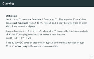
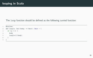
![Functions in Haskell
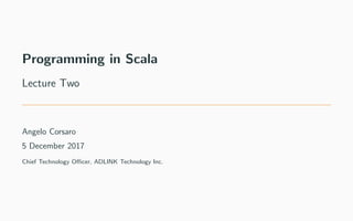
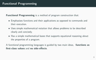
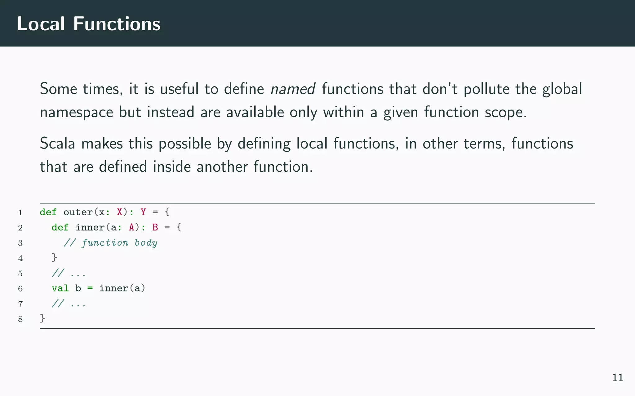
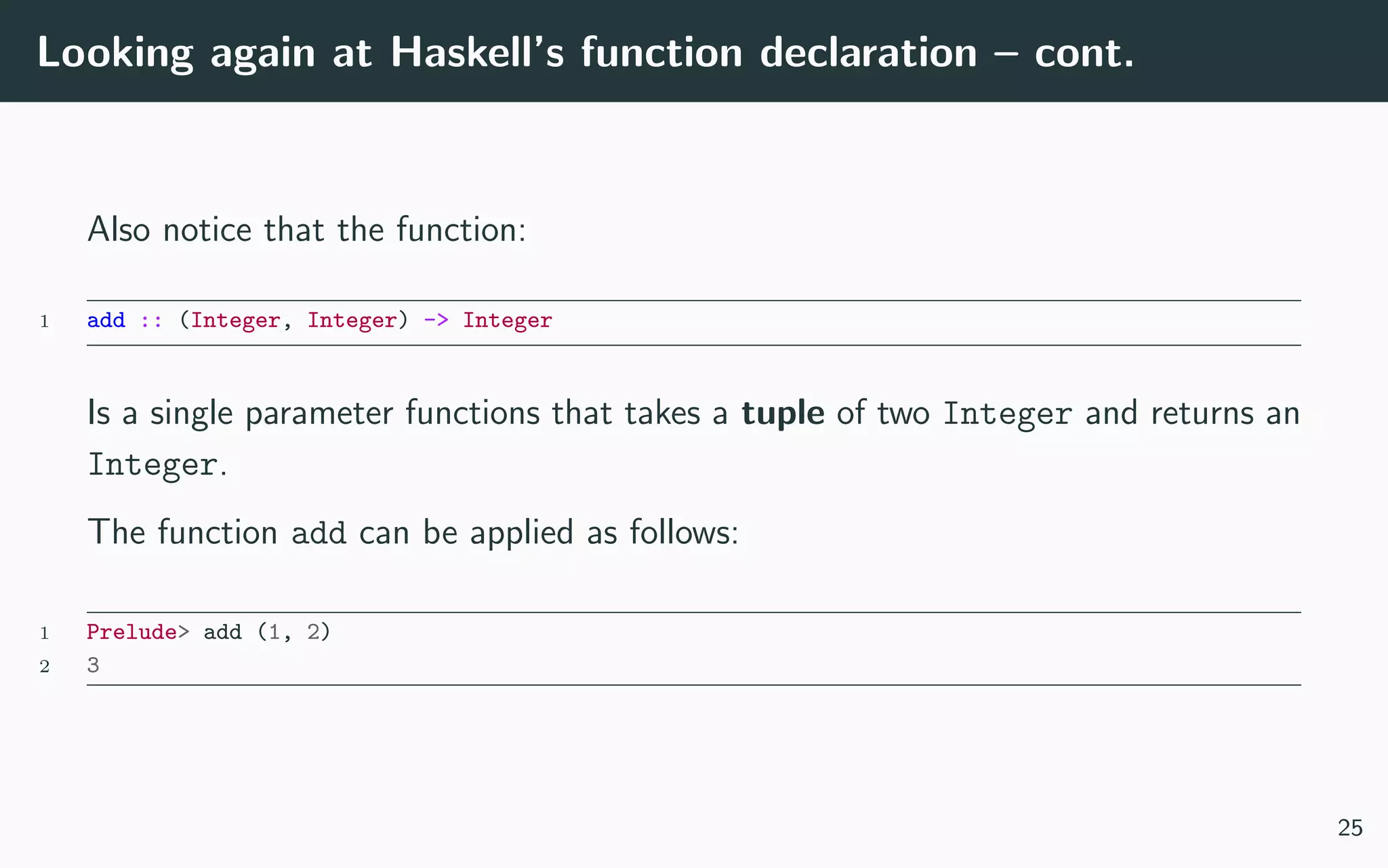
Haskell’s notation to denotate a function f that takes an argument of type X
and returns a result of type Y is:
1 f :: X -> Y
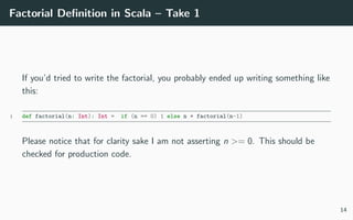
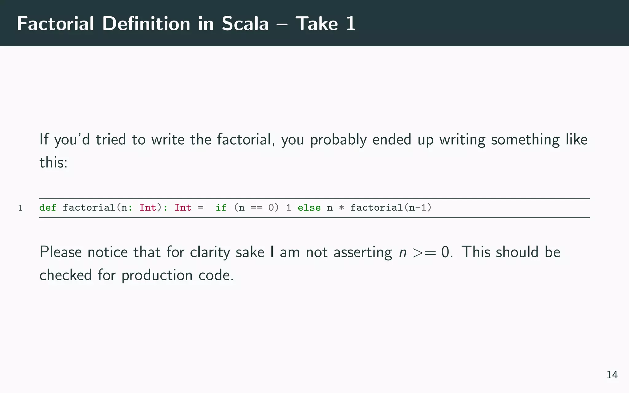
Example
For example:
1 sin :: Float -> Float
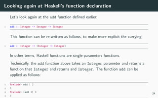
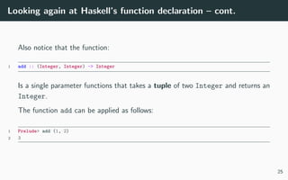
2 add :: Integer -> Integer -> Integer
3 reverse :: String -> String
4 sum :: [Integer] -> Integer
Notice how Haskell’s functions declaration is extremely close to that used in
mathematics. This is not accidental, and we will see the analogy goes quite far.
7](https://image.slidesharecdn.com/lecture-02-180109231409/85/Programming-in-Scala-Lecture-Two-11-320.jpg)
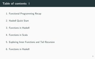
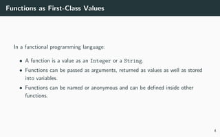
![Getting Started with Haskell
The best way to get started with Haskell is to unstall stack from
https://docs.haskellstack.org/en/stable/README/.
Once installed you can start Haskell’s REPL and experiment a bit:
1 > stack repl
2 Prelude> let xs = [1..10]
3 Prelude> :t xs
4 xs :: (Num t, Enum t) => [t]
5 Prelude> :t sum
6 sum :: (Num a, Foldable t) => t a -> a
7 Prelude> sum xs
8 55
9 Prelude> :t foldl
10 foldl :: Foldable t => (b -> a -> b) -> b -> t a -> b
11 Prelude> foldl (+) 0 xs
12 55
13 Prelude> foldl (*) 1 xs
14 3628800
8](https://image.slidesharecdn.com/lecture-02-180109231409/85/Programming-in-Scala-Lecture-Two-12-320.jpg)
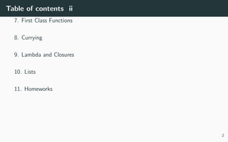
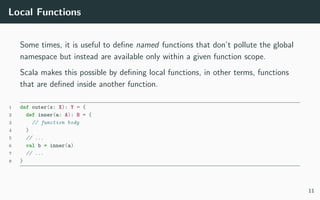
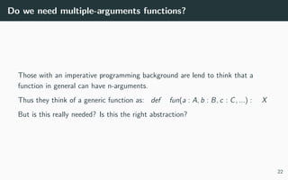
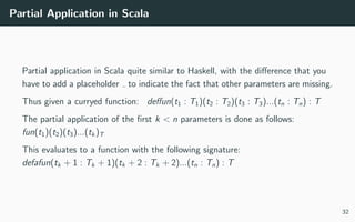
![Functions in Scala
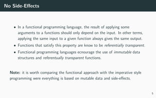
Scala’s notation to denotate a function f that takes an argument of type X and
returns a result of type Y is:
1 def f(x: X): Y
Example
For example:
1 def sin(x: Float): Float
2 def add(a: Integer, b: Integer): Integer
3 def reverse(s: String): String
4 def sum(xs: Array[Integer]): Integer
Notice how Haskell’s functions declaration is extremely close to that used in
mathematics. This is not accidental, and we will see the analogy goes quite far.
9](https://image.slidesharecdn.com/lecture-02-180109231409/85/Programming-in-Scala-Lecture-Two-14-320.jpg)
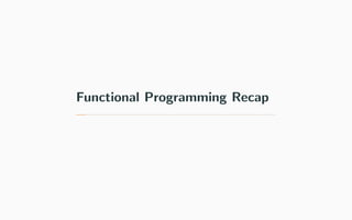
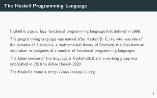
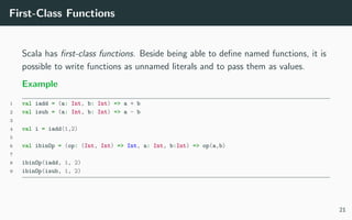
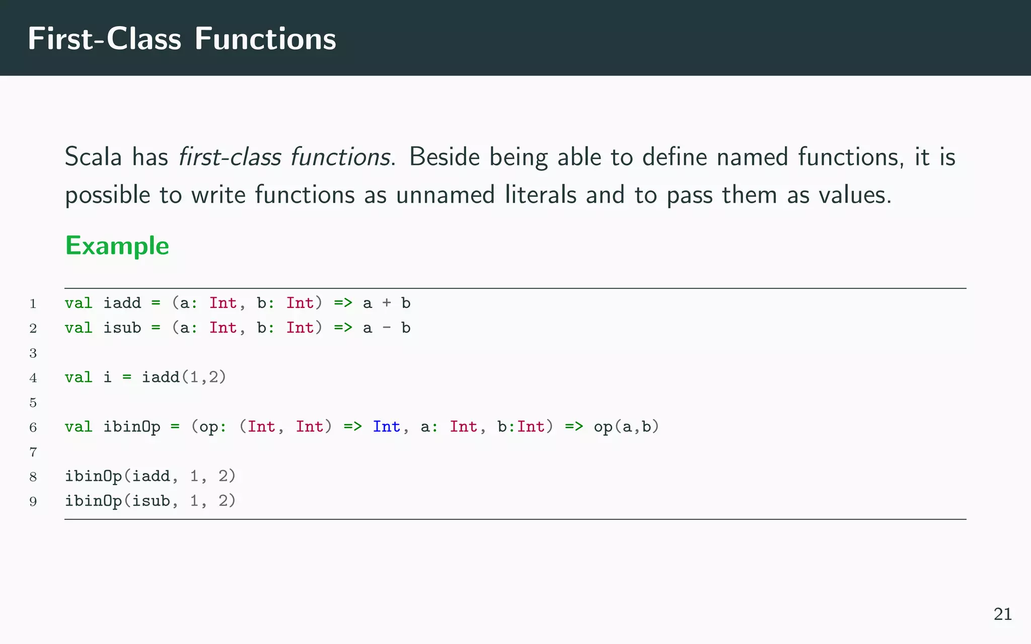
![Functions are Objects
In Scala function a function:
def f (t1 : T1, t2 : T2, ..., tn : Tn) : R
is are represented at runtime as objects whose type is:
trait Fun[−T1, −T2, ..., −Tn, +R] extends AnyRef
10](https://image.slidesharecdn.com/lecture-02-180109231409/85/Programming-in-Scala-Lecture-Two-15-320.jpg)


![Computing on Lists with Pattern Matching
1 val xs = List(1,2,3,4)
2
3 def sum(xs: List[Int]): Int = xs match {
4 case y::ys => y+sum(ys)
5 case List() => 0
6 }
7
8 def mul(xs: List[Int]): Int = xs match {
9 case y::ys => y*mul(ys)
10 case List() => 1
11 }
12
13 def reverse(xs: List[Int]): List[Int] = xs match {
14 case List() => List()
15 case y::ys => reverse(ys) ::: List(y)
16 }
40](https://image.slidesharecdn.com/lecture-02-180109231409/85/Programming-in-Scala-Lecture-Two-51-320.jpg)
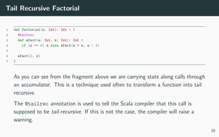
![Folding Lists
The functions we just wrote for lists can all be expressed in terms of fold
operator.
1 def sum(xs: List[Int]): Int = xs.foldRight(0)(_ + _)
2
3 def sum(xs: List[Int]): Int = xs.foldLeft(0)(_ + _)
4
5 def reversel(ys: List[Int])= ys.foldLeft(List[Int]())((xs: List[Int], x: Int) => x :: xs)
6
7 def reverser(ys: List[Int]) = zs.foldRight(List[Int]())((x: Int, xs: List[Int]) => xs ::: List(x) )
41](https://image.slidesharecdn.com/lecture-02-180109231409/85/Programming-in-Scala-Lecture-Two-52-320.jpg)

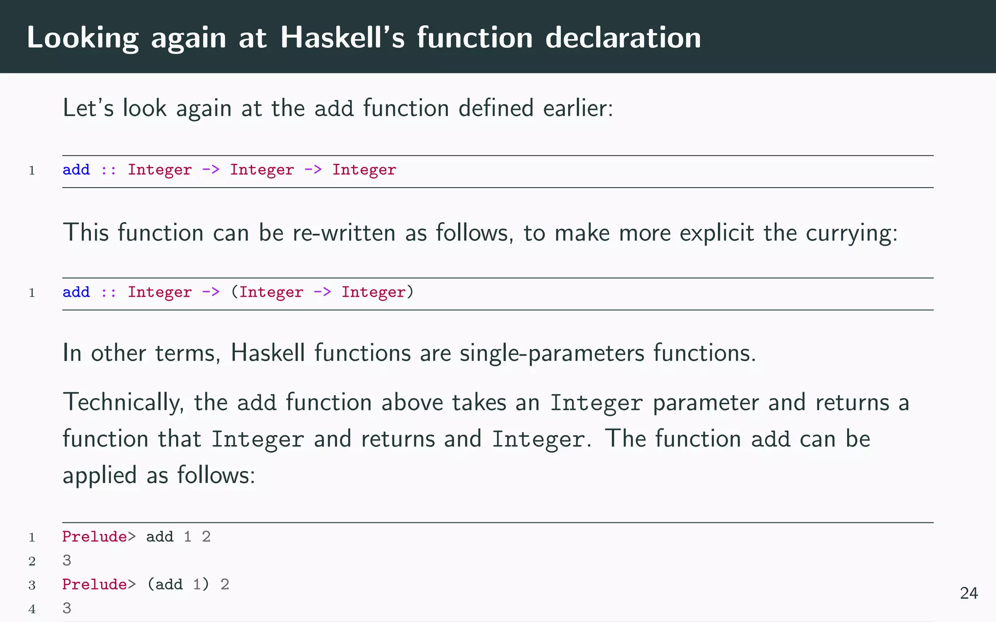
![Functions in Haskell
Haskell’s notation to denotate a function f that takes an argument of type X
and returns a result of type Y is:
1 f :: X -> Y
Example
For example:
1 sin :: Float -> Float
2 add :: Integer -> Integer -> Integer
3 reverse :: String -> String
4 sum :: [Integer] -> Integer
Notice how Haskell’s functions declaration is extremely close to that used in
mathematics. This is not accidental, and we will see the analogy goes quite far.
7](https://image.slidesharecdn.com/lecture-02-180109231409/75/Programming-in-Scala-Lecture-Two-11-2048.jpg)
![Getting Started with Haskell
The best way to get started with Haskell is to unstall stack from
https://docs.haskellstack.org/en/stable/README/.
Once installed you can start Haskell’s REPL and experiment a bit:
1 > stack repl
2 Prelude> let xs = [1..10]
3 Prelude> :t xs
4 xs :: (Num t, Enum t) => [t]
5 Prelude> :t sum
6 sum :: (Num a, Foldable t) => t a -> a
7 Prelude> sum xs
8 55
9 Prelude> :t foldl
10 foldl :: Foldable t => (b -> a -> b) -> b -> t a -> b
11 Prelude> foldl (+) 0 xs
12 55
13 Prelude> foldl (*) 1 xs
14 3628800
8](https://image.slidesharecdn.com/lecture-02-180109231409/75/Programming-in-Scala-Lecture-Two-12-2048.jpg)
![Functions in Scala
Scala’s notation to denotate a function f that takes an argument of type X and
returns a result of type Y is:
1 def f(x: X): Y
Example
For example:
1 def sin(x: Float): Float
2 def add(a: Integer, b: Integer): Integer
3 def reverse(s: String): String
4 def sum(xs: Array[Integer]): Integer
Notice how Haskell’s functions declaration is extremely close to that used in
mathematics. This is not accidental, and we will see the analogy goes quite far.
9](https://image.slidesharecdn.com/lecture-02-180109231409/75/Programming-in-Scala-Lecture-Two-14-2048.jpg)
![Functions are Objects
In Scala function a function:
def f (t1 : T1, t2 : T2, ..., tn : Tn) : R
is are represented at runtime as objects whose type is:
trait Fun[−T1, −T2, ..., −Tn, +R] extends AnyRef
10](https://image.slidesharecdn.com/lecture-02-180109231409/75/Programming-in-Scala-Lecture-Two-15-2048.jpg)


![Computing on Lists with Pattern Matching
1 val xs = List(1,2,3,4)
2
3 def sum(xs: List[Int]): Int = xs match {
4 case y::ys => y+sum(ys)
5 case List() => 0
6 }
7
8 def mul(xs: List[Int]): Int = xs match {
9 case y::ys => y*mul(ys)
10 case List() => 1
11 }
12
13 def reverse(xs: List[Int]): List[Int] = xs match {
14 case List() => List()
15 case y::ys => reverse(ys) ::: List(y)
16 }
40](https://image.slidesharecdn.com/lecture-02-180109231409/75/Programming-in-Scala-Lecture-Two-51-2048.jpg)
![Folding Lists
The functions we just wrote for lists can all be expressed in terms of fold
operator.
1 def sum(xs: List[Int]): Int = xs.foldRight(0)(_ + _)
2
3 def sum(xs: List[Int]): Int = xs.foldLeft(0)(_ + _)
4
5 def reversel(ys: List[Int])= ys.foldLeft(List[Int]())((xs: List[Int], x: Int) => x :: xs)
6
7 def reverser(ys: List[Int]) = zs.foldRight(List[Int]())((x: Int, xs: List[Int]) => xs ::: List(x) )
41](https://image.slidesharecdn.com/lecture-02-180109231409/75/Programming-in-Scala-Lecture-Two-52-2048.jpg)

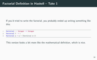
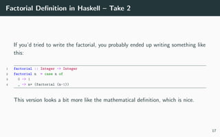
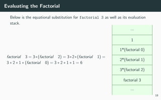
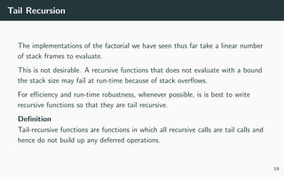
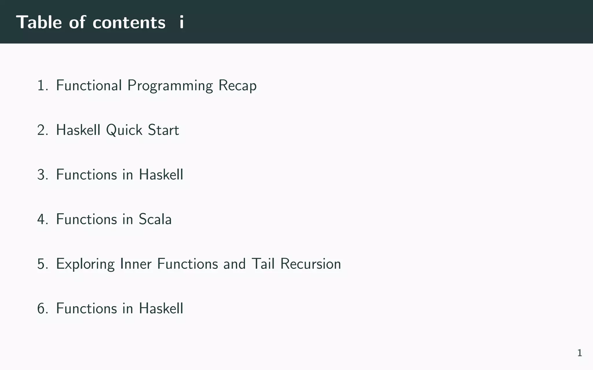
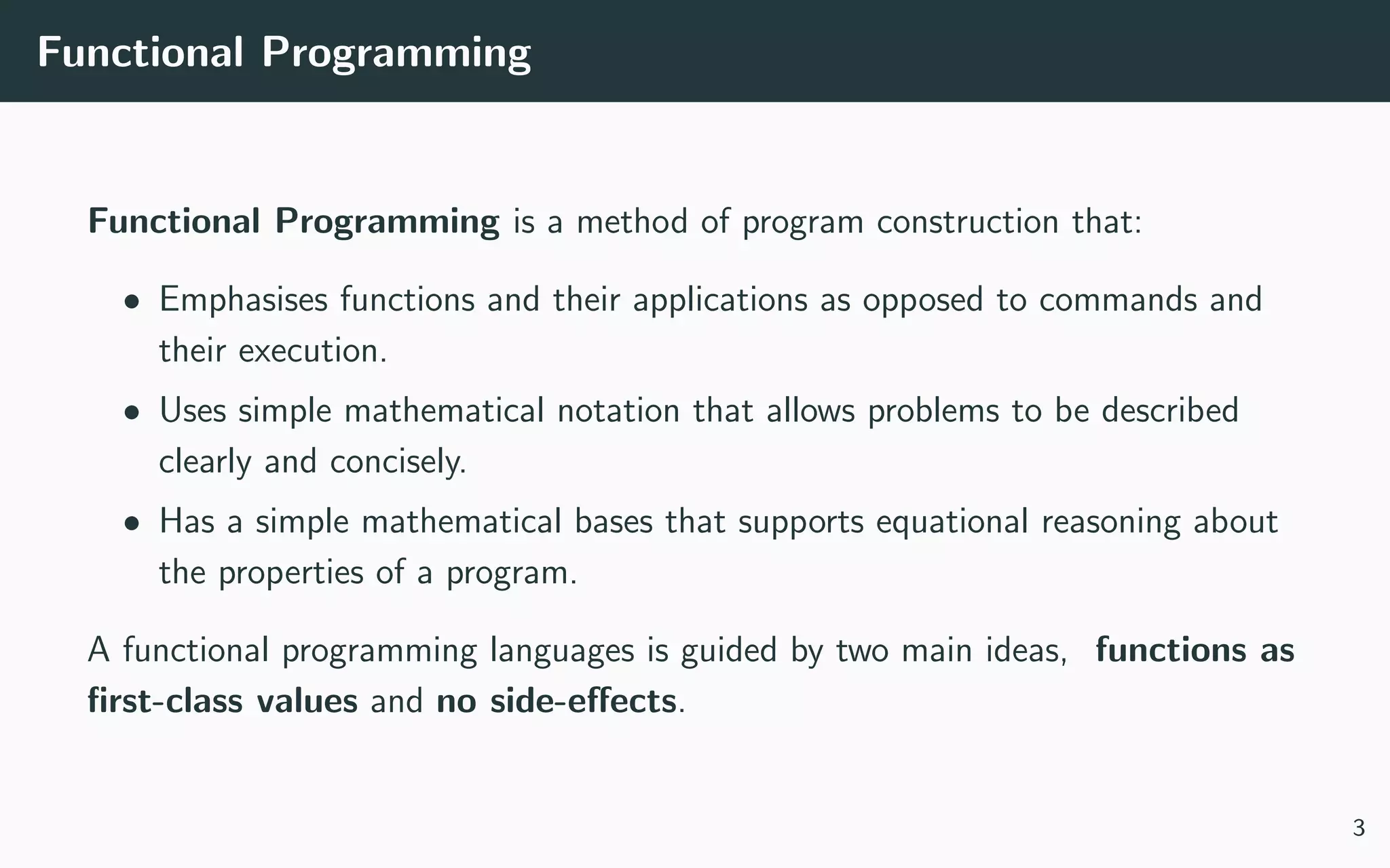
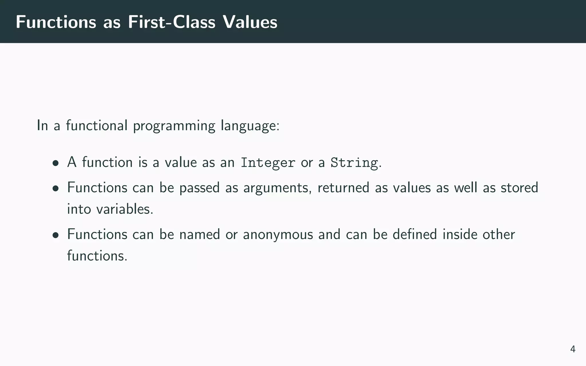
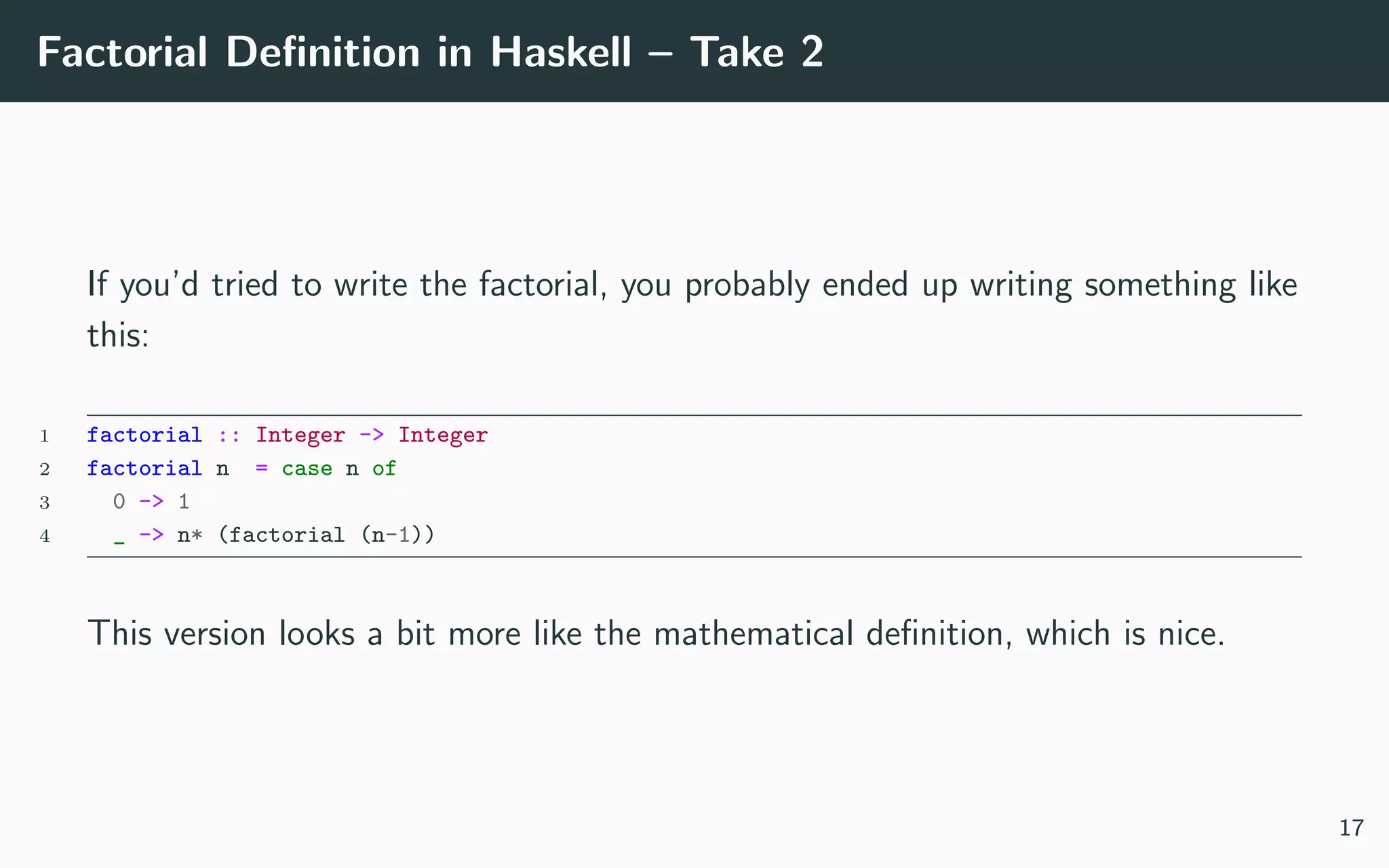
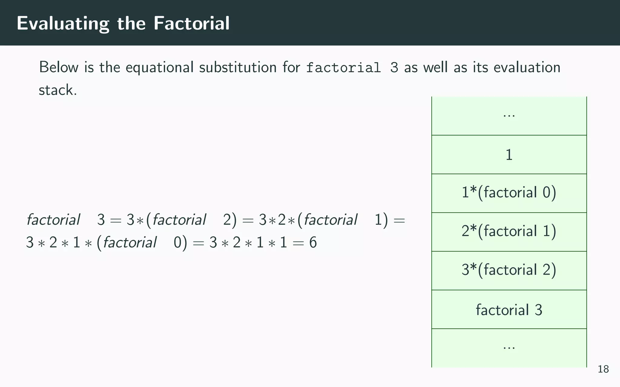
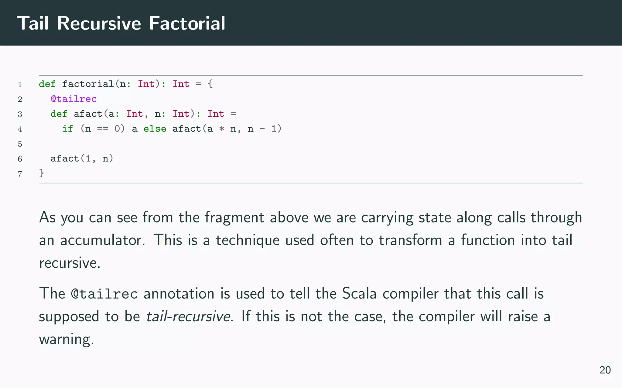
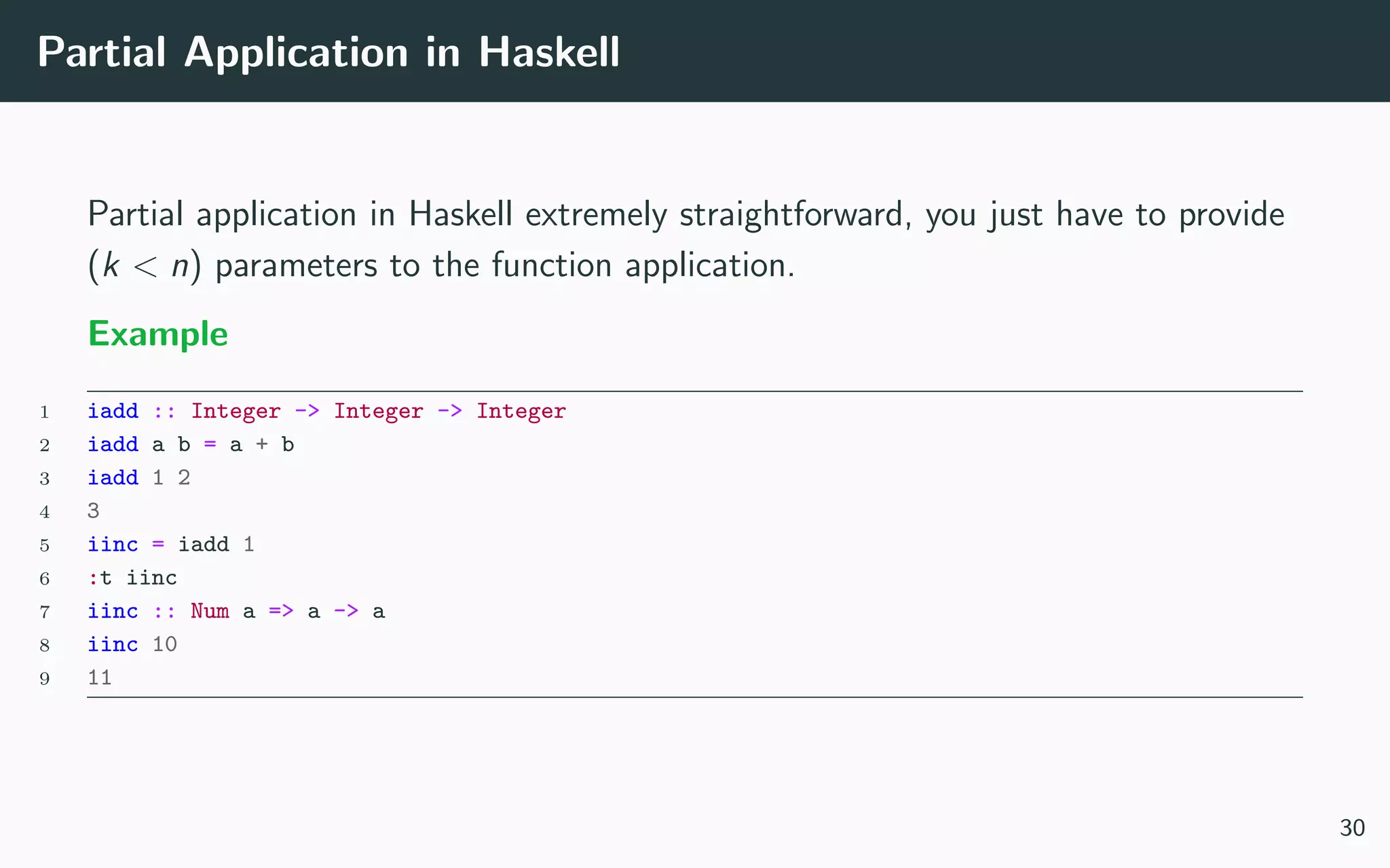
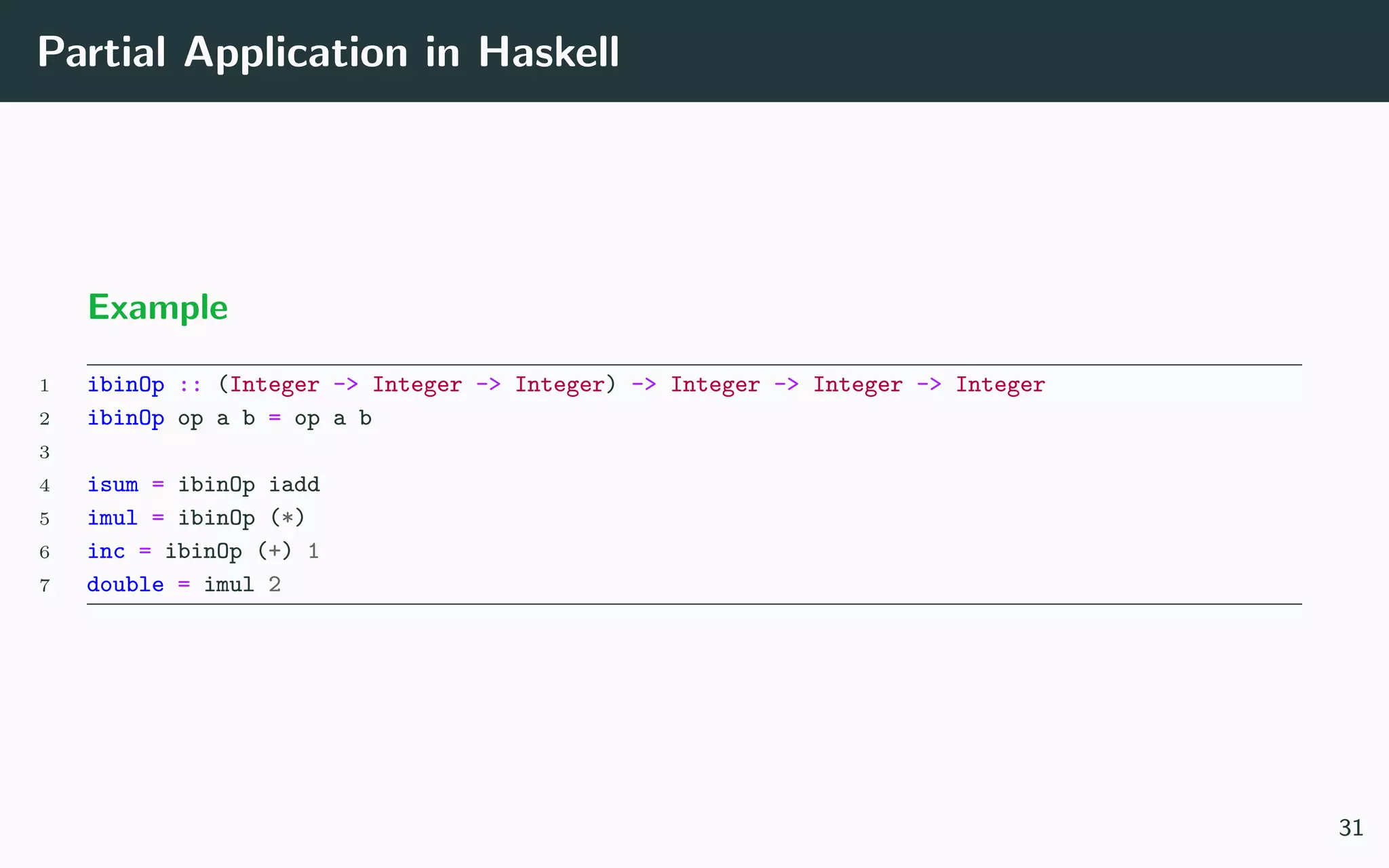
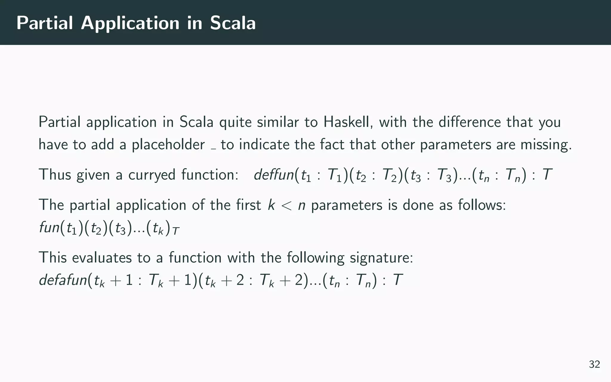
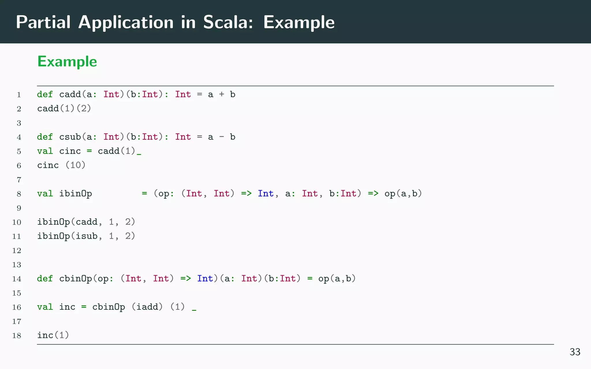
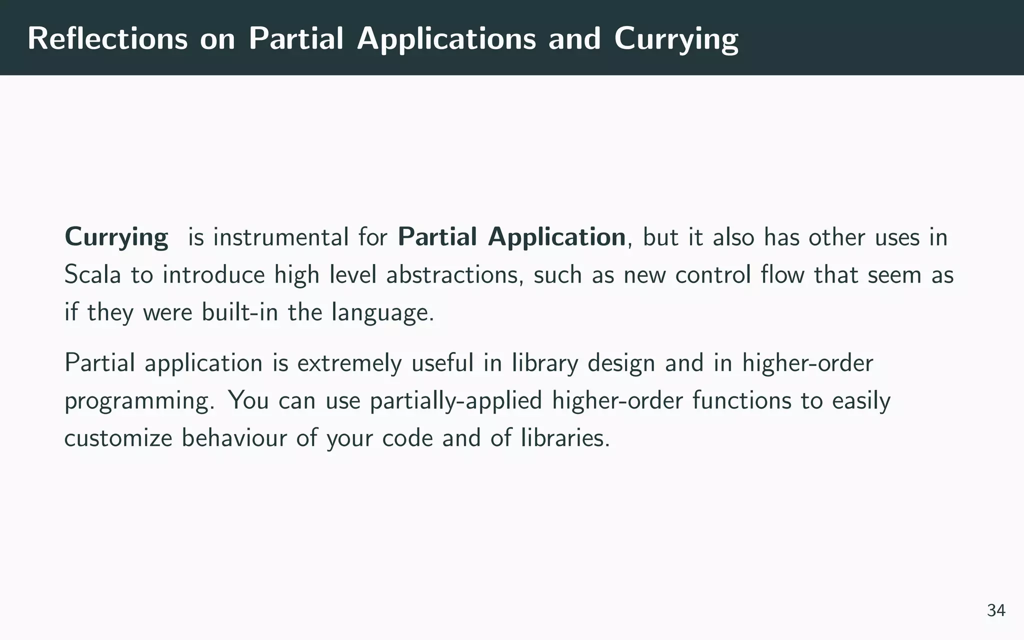
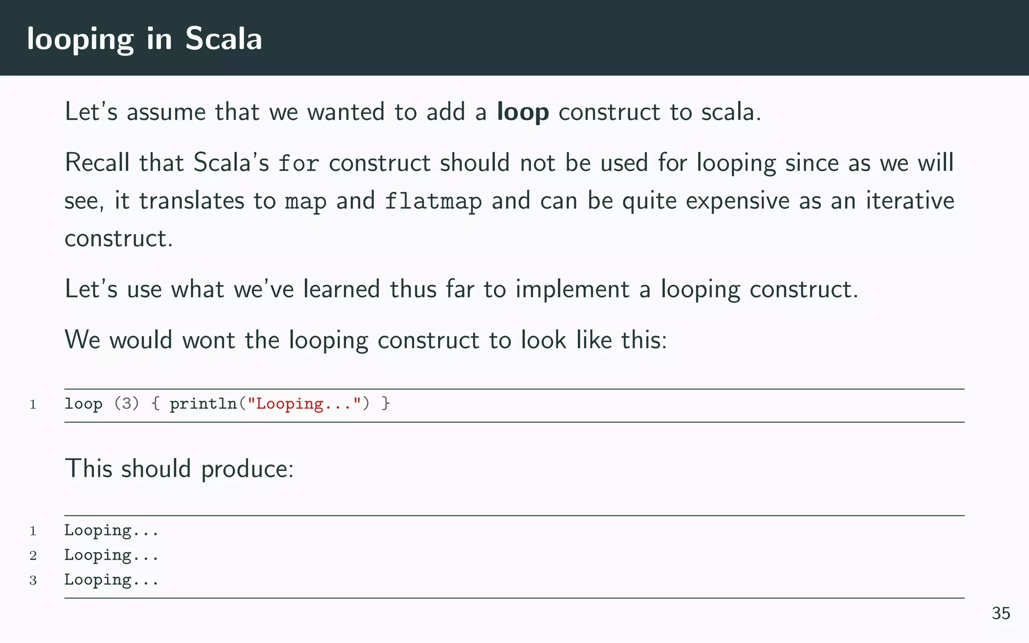
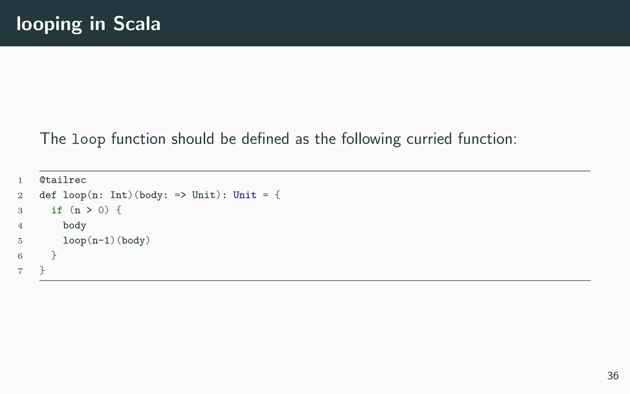
This document provides an overview of a lecture on functional programming in Scala. It covers the following topics: 1. A recap of functional programming principles like functions as first-class values and no side effects. 2. An introduction to the Haskell programming language including its syntax for defining functions. 3. How functions are defined in Scala and how they are objects at runtime. 4. Examples of defining the factorial function recursively in Haskell and Scala, and making it tail recursive. 5. Concepts of first-class functions, currying, partial application, and an example of implementing looping in Scala using these techniques.


![[FLOLAC'14][scm] Functional Programming Using Haskell](https://cdn.slidesharecdn.com/ss_thumbnails/slides-140630030216-phpapp01-thumbnail.jpg?width=600ounds&width=560&fit=bounds)


![UiPath Automation Suite Installation (Hands-On) [2/3]](https://cdn.slidesharecdn.com/ss_thumbnails/automationsuitecommunitysession2-251015095633-a6d862f1-thumbnail.jpg?width=600ounds&width=560&fit=bounds)


