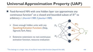
Download as PDF, PPTX


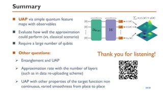
![QNN via Quantum Feature Map[1,2]
3/20
[1] V. Havlíček et al., Supervised Learning with Quantum-Enhanced Feature Spaces, Nature 567, 209 (2019)
[2] M. Schuld and N. Killoran, Quantum Machine Learning in Feature Hilbert Spaces, Phys. Rev. Lett. 122, 040504 (2019)
[3] Y. Liu et al., A Rigorous and Robust Quantum Speed-Up in Supervised Machine Learning, Nat. Phys. 17, 1013 (2021)
Input Space 𝒳
Quantum
Hilbert space
𝒙
|Ψ 𝒙 ⟩
Access via Measurements
or Compute Kernel
Or at least the same
expressivity as classical
𝜅 𝒙, 𝒙′ = ⟨Ψ(𝒙)|Ψ(𝒙′)⟩
Heuristic
Quantum Circuit Learning
(K. Mitarai, M. Negoro,M. Kitagawa,
and K. Fujii, Phys. Rev.A 98, 032309)
◼ For a special problem, a formal quantum advantage[3] can
be proven (but is neither “near-term” nor practical)
◼ We expect quantum feature maps to be more
expressive than classical counter parts](https://image.slidesharecdn.com/qtmlquapriken202111-211113065158/85/QTML2021-UAP-Quantum-Feature-Map-3-320.jpg)
![QNN via Quantum Feature Map
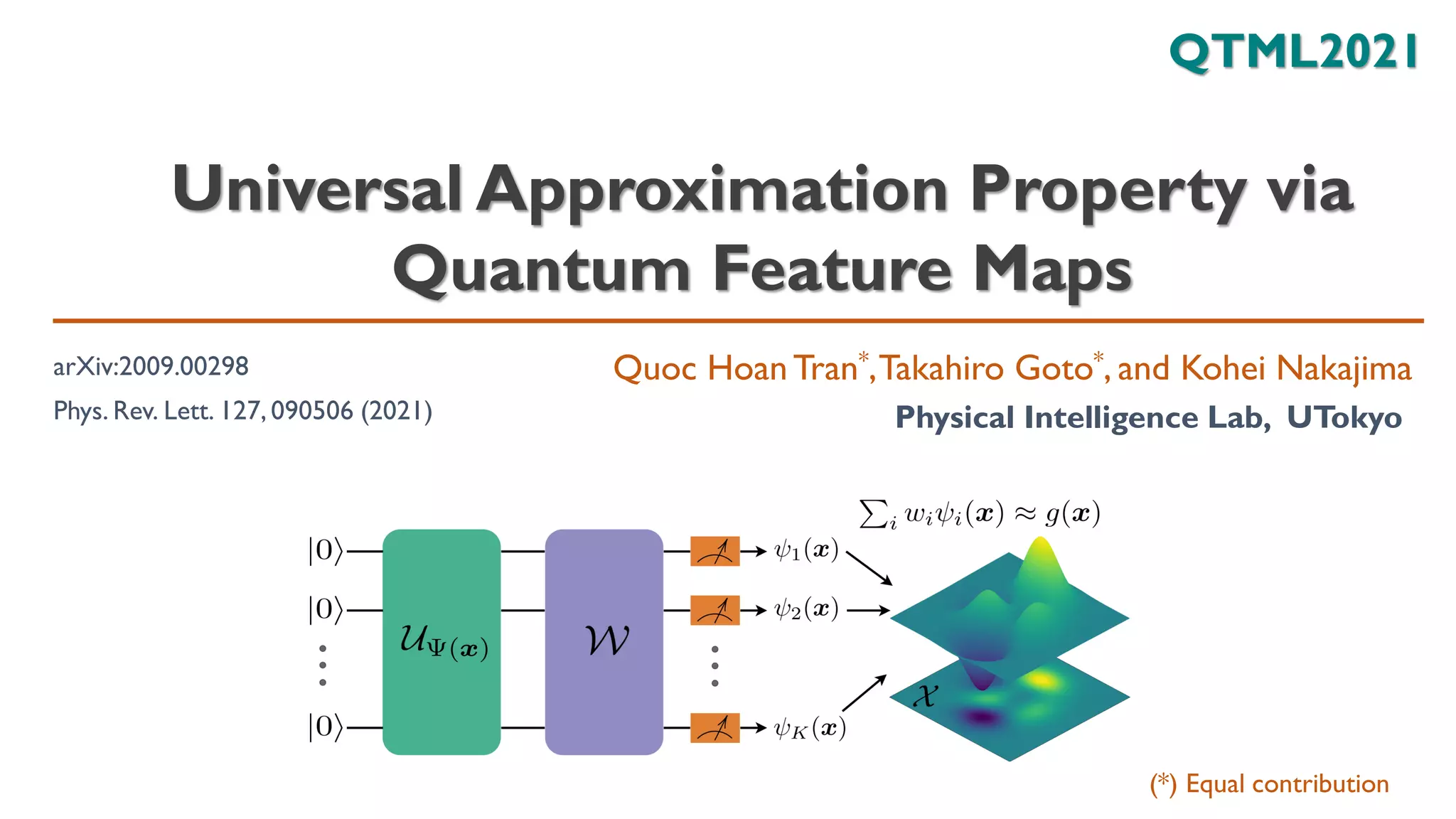
◼ Choosing W is equivalent to selecting suitable observables
6/20
◼ The output is a linear expansion of the basis functions with a
suitable set of observables
𝜓𝑖 𝒙 = Ψ 𝒙 𝑂𝑖 Ψ 𝒙 𝑓 𝒙; Ψ, 𝑶, 𝒘 =
𝑖=1
𝐾
𝑤𝑖𝜓𝑖 𝒙
[1]V. Havlíček et al., Supervised Learning with Quantum-Enhanced Feature Spaces, Nature 567, 209 (2019)
𝑤𝛽 𝜽 = Tr 𝒲† 𝜽 𝑍⊗𝑁𝒲 𝜽 𝑃𝛽 𝑃𝛽 ∈ 𝐼, 𝑋, 𝑌, 𝑍 ⊗𝑁
𝜓𝛽 𝒙 = Tr Ψ 𝒙 Ψ 𝒙 𝑃𝛽
Pauli-group
Basis functions (expectation)
E.g., Decision function[1] sign
1
2𝑁
𝛽
𝑤𝛽 𝜽 𝜓𝛽 𝒙 + 𝑏](https://image.slidesharecdn.com/qtmlquapriken202111-211113065158/85/QTML2021-UAP-Quantum-Feature-Map-6-320.jpg)

![Parallel scenario
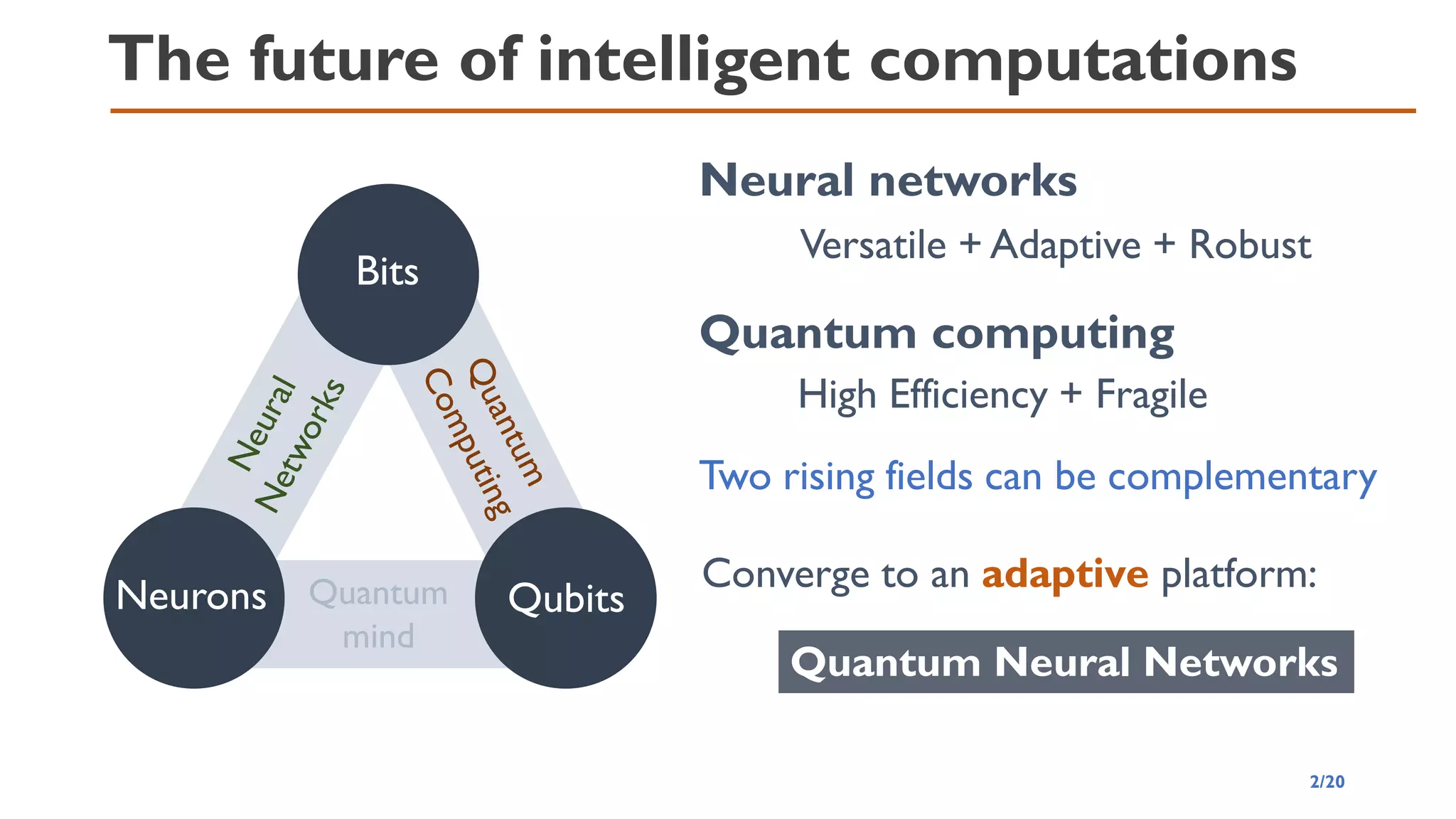
Approach 1. Produce the “nonlinear” by suitable observables
◼ Basis functions can be polynomials if we choose the
correlated measurement operators
◼ Then we apply the Weierstrass’s polynomial approximation
theorem
𝑈𝑁 𝒙 = 𝑉1 𝒙 ⊗ ⋯ ⊗ 𝑉𝑁 𝒙
𝑉
𝑗 𝒙 = 𝑒−𝑗𝜃𝑗 𝒙 𝑌 𝜃𝑗 𝒙 = arccos( 𝑥𝑘) for 1 ≤ 𝑘 ≤ 𝑑, 𝑗 ≡ 𝑘(mod 𝑑)
𝑂𝒂 = 𝑍𝑎1 ⊗ ⋯ ⊗ 𝑍𝑎𝑁, 𝒂 ∈ 0,1 𝑁
Observables
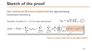
Basis functions 𝜓𝒂 𝑥 = Ψ𝑁 𝒙 𝑂𝒂 Ψ𝑁 𝒙 = ෑ
𝑖=1
𝑁
2𝑥[𝑖] − 1
𝑎𝑖
Feature map: Ψ𝑁(𝒙) = 𝑈𝑁 𝒙 0 ⊗𝑁
1 ≤ 𝑖 ≤ 𝑑
𝑖 ≡ 𝑖 (𝑚𝑜𝑑 𝑑)
9/20](https://image.slidesharecdn.com/qtmlquapriken202111-211113065158/85/QTML2021-UAP-Quantum-Feature-Map-9-320.jpg)
![Parallel scenario
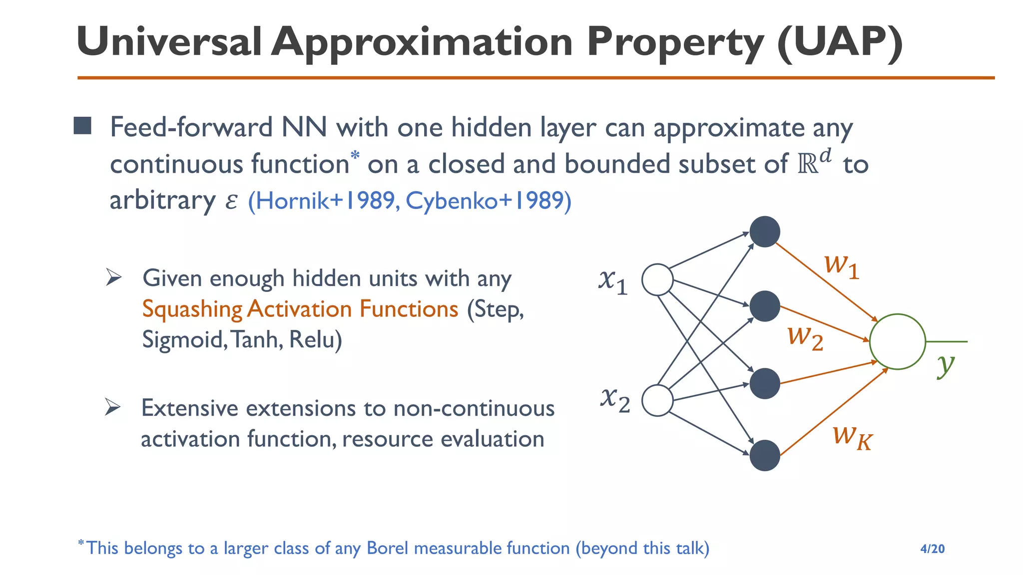
Approach 2. Activation function in pre-processing (straight-forward)
[Huang+, Neurocomputing, 2007] 𝜎: 𝑅 → [−1,1] is nonconstant piecewise continuous function
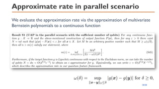
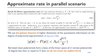
such that 𝜎(𝒂 ⋅ 𝒙 + 𝒃) is dense in 𝐿2(𝑋).Then, for any continuous function 𝑔: 𝑋 → 𝑅 and any
function sequence 𝜎𝑗 𝒙 = 𝜎 𝒂𝑗 ⋅ 𝒙 + 𝑏𝑗 where 𝒂𝑗, 𝑏𝑗 are randomly generated based on any
continuous sampling distribution,
lim
𝑁→∞
min
𝒘
𝑗
𝑁
𝑤𝑗𝜎𝑗 𝒙 − 𝑔(𝒙)
𝐿2
= 0
We obtain UAP if we can implement the squashing activation function in
pre-processing process (Result 2)
• 𝑈𝑁 𝒙 = 𝑉1 𝒙 ⊗ ⋯ ⊗ 𝑉𝑁 𝒙
• 𝑉
𝑗 𝒙 = 𝑒−𝑗𝜃𝑗 𝒙 𝑌
• 𝜃𝑗 𝒙 = arccos(
1+𝜎(𝒂𝑗⋅𝒙+𝑏𝑗)
2
)
𝜓𝑗 𝑥 = Ψ𝑁 𝒙 𝑍𝑗 Ψ𝑁 𝒙 = ⟨0|𝑒𝑖𝜃𝑗𝑌
𝑍𝑒−𝑖𝜃𝑗𝑌
|0⟩
= 2 cos2(𝜃𝑗) − 1 = 𝜎 𝒂𝑗 ⋅ 𝒙 + 𝑏𝑗 = 𝜎𝑗(𝒙)
11/20](https://image.slidesharecdn.com/qtmlquapriken202111-211113065158/85/QTML2021-UAP-Quantum-Feature-Map-11-320.jpg)

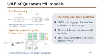
![UAP – Approximation Rate
Classical UAP of DNN
inf
𝐰
𝑓
𝒘 − 𝑔 = 𝑂(𝐾−𝛽/𝑑
)
[1] Hrushiksh M Mhaskar. Neural networks for optimal approximation of smooth and analytic functions. Neural Computation, 8(1):164-167, 1996
Optimal rate[3]
[2] Dmitry Yarotsky. Error bounds for approximations with deep Relu networks. Neural Networks, 94:103-114, 2017
[3] Ronald A DeVore. Optimal nonlinear approximation. Manuscripta Mathematica, 63(4):469-478, 1989.
𝐾
𝜀
𝑂(𝐾−𝛼1)
𝑂(𝐾−𝛼2)
𝛼1 < 𝛼2
13/20
The following statement[1,2] holds for continuous activation
function (with 𝐿 = 2), and ReLU (with 𝐿 = 𝑂(𝛽log
𝐾
𝑑
))
➢ 𝑑: input dimension
➢ 𝐾: number of network parameters
➢ 𝛽: derivative order of g
➢ 𝐿: number of layers.
How to describe relative good and bad UAP?
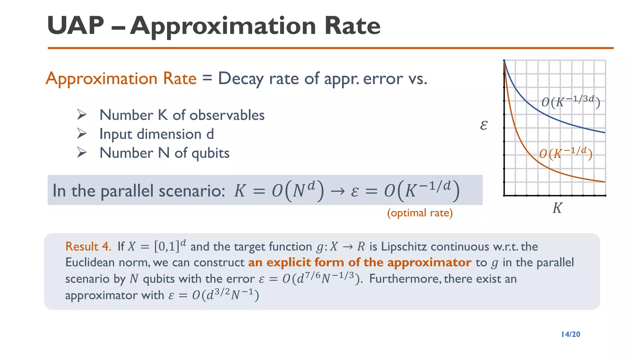
Approximation Rate = Decay rate of appr. error vs.
(better rate)](https://image.slidesharecdn.com/qtmlquapriken202111-211113065158/85/QTML2021-UAP-Quantum-Feature-Map-13-320.jpg)


![QNN via Quantum Feature Map[1,2]
3/20
[1] V. Havlíček et al., Supervised Learning with Quantum-Enhanced Feature Spaces, Nature 567, 209 (2019)
[2] M. Schuld and N. Killoran, Quantum Machine Learning in Feature Hilbert Spaces, Phys. Rev. Lett. 122, 040504 (2019)
[3] Y. Liu et al., A Rigorous and Robust Quantum Speed-Up in Supervised Machine Learning, Nat. Phys. 17, 1013 (2021)
Input Space 𝒳
Quantum
Hilbert space
𝒙
|Ψ 𝒙 ⟩
Access via Measurements
or Compute Kernel
Or at least the same
expressivity as classical
𝜅 𝒙, 𝒙′ = ⟨Ψ(𝒙)|Ψ(𝒙′)⟩
Heuristic
Quantum Circuit Learning
(K. Mitarai, M. Negoro,M. Kitagawa,
and K. Fujii, Phys. Rev.A 98, 032309)
◼ For a special problem, a formal quantum advantage[3] can
be proven (but is neither “near-term” nor practical)
◼ We expect quantum feature maps to be more
expressive than classical counter parts](https://image.slidesharecdn.com/qtmlquapriken202111-211113065158/75/QTML2021-UAP-Quantum-Feature-Map-3-2048.jpg)
![QNN via Quantum Feature Map
◼ Choosing W is equivalent to selecting suitable observables
6/20
◼ The output is a linear expansion of the basis functions with a
suitable set of observables
𝜓𝑖 𝒙 = Ψ 𝒙 𝑂𝑖 Ψ 𝒙 𝑓 𝒙; Ψ, 𝑶, 𝒘 =
𝑖=1
𝐾
𝑤𝑖𝜓𝑖 𝒙
[1]V. Havlíček et al., Supervised Learning with Quantum-Enhanced Feature Spaces, Nature 567, 209 (2019)
𝑤𝛽 𝜽 = Tr 𝒲† 𝜽 𝑍⊗𝑁𝒲 𝜽 𝑃𝛽 𝑃𝛽 ∈ 𝐼, 𝑋, 𝑌, 𝑍 ⊗𝑁
𝜓𝛽 𝒙 = Tr Ψ 𝒙 Ψ 𝒙 𝑃𝛽
Pauli-group
Basis functions (expectation)
E.g., Decision function[1] sign
1
2𝑁
𝛽
𝑤𝛽 𝜽 𝜓𝛽 𝒙 + 𝑏](https://image.slidesharecdn.com/qtmlquapriken202111-211113065158/75/QTML2021-UAP-Quantum-Feature-Map-6-2048.jpg)
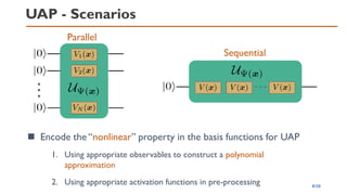
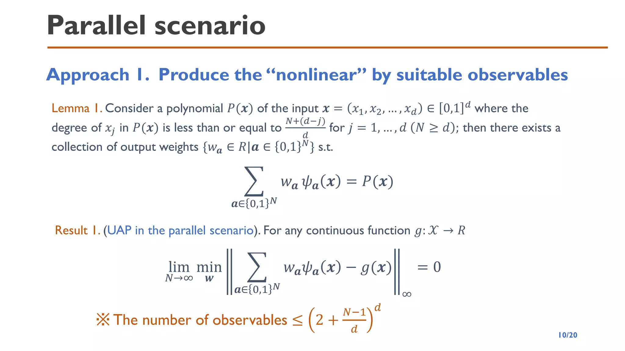
![Parallel scenario
Approach 1. Produce the “nonlinear” by suitable observables
◼ Basis functions can be polynomials if we choose the
correlated measurement operators
◼ Then we apply the Weierstrass’s polynomial approximation
theorem
𝑈𝑁 𝒙 = 𝑉1 𝒙 ⊗ ⋯ ⊗ 𝑉𝑁 𝒙
𝑉
𝑗 𝒙 = 𝑒−𝑗𝜃𝑗 𝒙 𝑌 𝜃𝑗 𝒙 = arccos( 𝑥𝑘) for 1 ≤ 𝑘 ≤ 𝑑, 𝑗 ≡ 𝑘(mod 𝑑)
𝑂𝒂 = 𝑍𝑎1 ⊗ ⋯ ⊗ 𝑍𝑎𝑁, 𝒂 ∈ 0,1 𝑁
Observables
Basis functions 𝜓𝒂 𝑥 = Ψ𝑁 𝒙 𝑂𝒂 Ψ𝑁 𝒙 = ෑ
𝑖=1
𝑁
2𝑥[𝑖] − 1
𝑎𝑖
Feature map: Ψ𝑁(𝒙) = 𝑈𝑁 𝒙 0 ⊗𝑁
1 ≤ 𝑖 ≤ 𝑑
𝑖 ≡ 𝑖 (𝑚𝑜𝑑 𝑑)
9/20](https://image.slidesharecdn.com/qtmlquapriken202111-211113065158/75/QTML2021-UAP-Quantum-Feature-Map-9-2048.jpg)
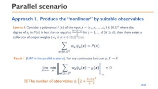
![Parallel scenario
Approach 2. Activation function in pre-processing (straight-forward)
[Huang+, Neurocomputing, 2007] 𝜎: 𝑅 → [−1,1] is nonconstant piecewise continuous function
such that 𝜎(𝒂 ⋅ 𝒙 + 𝒃) is dense in 𝐿2(𝑋).Then, for any continuous function 𝑔: 𝑋 → 𝑅 and any
function sequence 𝜎𝑗 𝒙 = 𝜎 𝒂𝑗 ⋅ 𝒙 + 𝑏𝑗 where 𝒂𝑗, 𝑏𝑗 are randomly generated based on any
continuous sampling distribution,
lim
𝑁→∞
min
𝒘
𝑗
𝑁
𝑤𝑗𝜎𝑗 𝒙 − 𝑔(𝒙)
𝐿2
= 0
We obtain UAP if we can implement the squashing activation function in
pre-processing process (Result 2)
• 𝑈𝑁 𝒙 = 𝑉1 𝒙 ⊗ ⋯ ⊗ 𝑉𝑁 𝒙
• 𝑉
𝑗 𝒙 = 𝑒−𝑗𝜃𝑗 𝒙 𝑌
• 𝜃𝑗 𝒙 = arccos(
1+𝜎(𝒂𝑗⋅𝒙+𝑏𝑗)
2
)
𝜓𝑗 𝑥 = Ψ𝑁 𝒙 𝑍𝑗 Ψ𝑁 𝒙 = ⟨0|𝑒𝑖𝜃𝑗𝑌
𝑍𝑒−𝑖𝜃𝑗𝑌
|0⟩
= 2 cos2(𝜃𝑗) − 1 = 𝜎 𝒂𝑗 ⋅ 𝒙 + 𝑏𝑗 = 𝜎𝑗(𝒙)
11/20](https://image.slidesharecdn.com/qtmlquapriken202111-211113065158/75/QTML2021-UAP-Quantum-Feature-Map-11-2048.jpg)
![UAP – Approximation Rate
Classical UAP of DNN
inf
𝐰
𝑓
𝒘 − 𝑔 = 𝑂(𝐾−𝛽/𝑑
)
[1] Hrushiksh M Mhaskar. Neural networks for optimal approximation of smooth and analytic functions. Neural Computation, 8(1):164-167, 1996
Optimal rate[3]
[2] Dmitry Yarotsky. Error bounds for approximations with deep Relu networks. Neural Networks, 94:103-114, 2017
[3] Ronald A DeVore. Optimal nonlinear approximation. Manuscripta Mathematica, 63(4):469-478, 1989.
𝐾
𝜀
𝑂(𝐾−𝛼1)
𝑂(𝐾−𝛼2)
𝛼1 < 𝛼2
13/20
The following statement[1,2] holds for continuous activation
function (with 𝐿 = 2), and ReLU (with 𝐿 = 𝑂(𝛽log
𝐾
𝑑
))
➢ 𝑑: input dimension
➢ 𝐾: number of network parameters
➢ 𝛽: derivative order of g
➢ 𝐿: number of layers.
How to describe relative good and bad UAP?
Approximation Rate = Decay rate of appr. error vs.
(better rate)](https://image.slidesharecdn.com/qtmlquapriken202111-211113065158/75/QTML2021-UAP-Quantum-Feature-Map-13-2048.jpg)

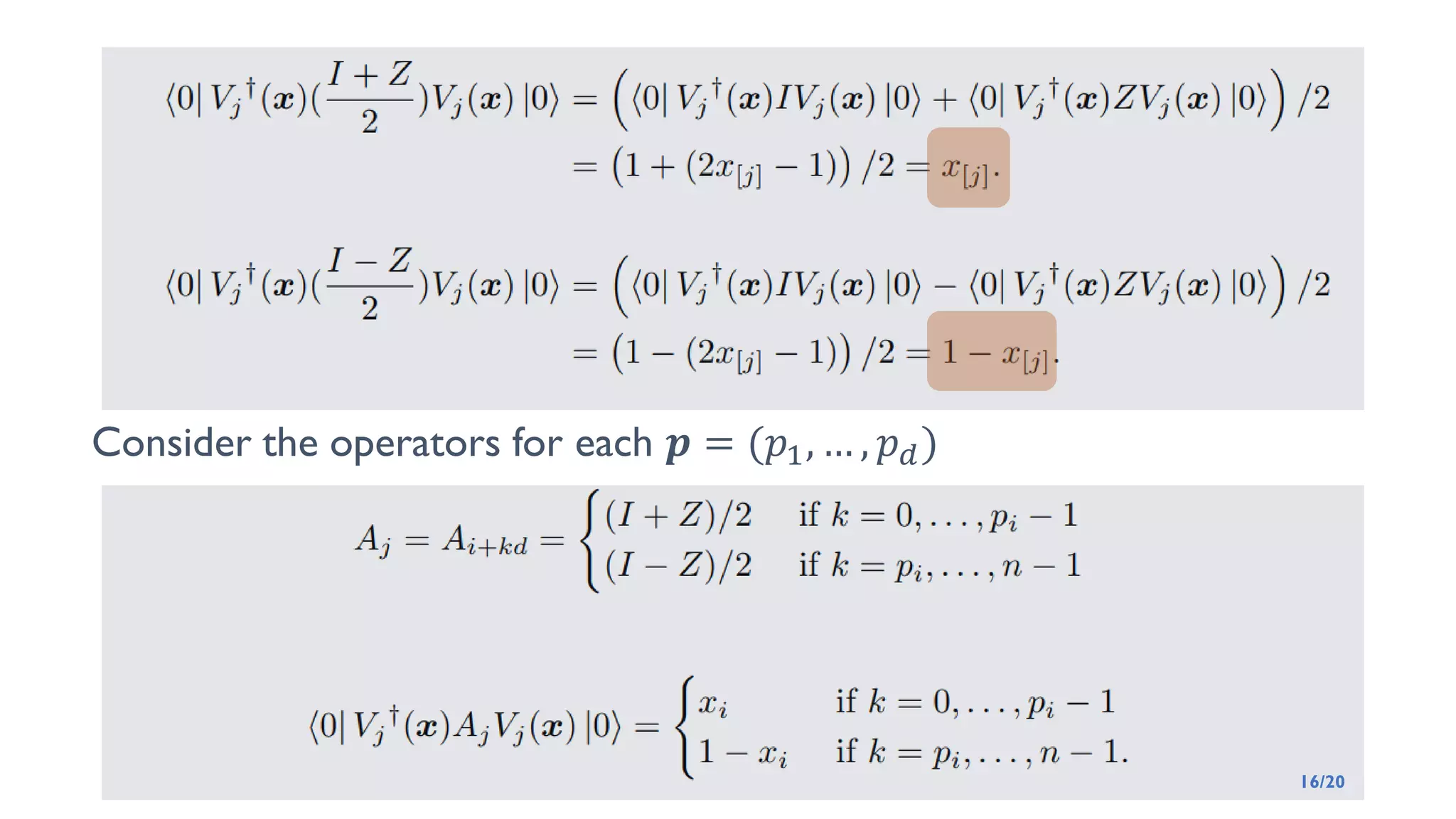
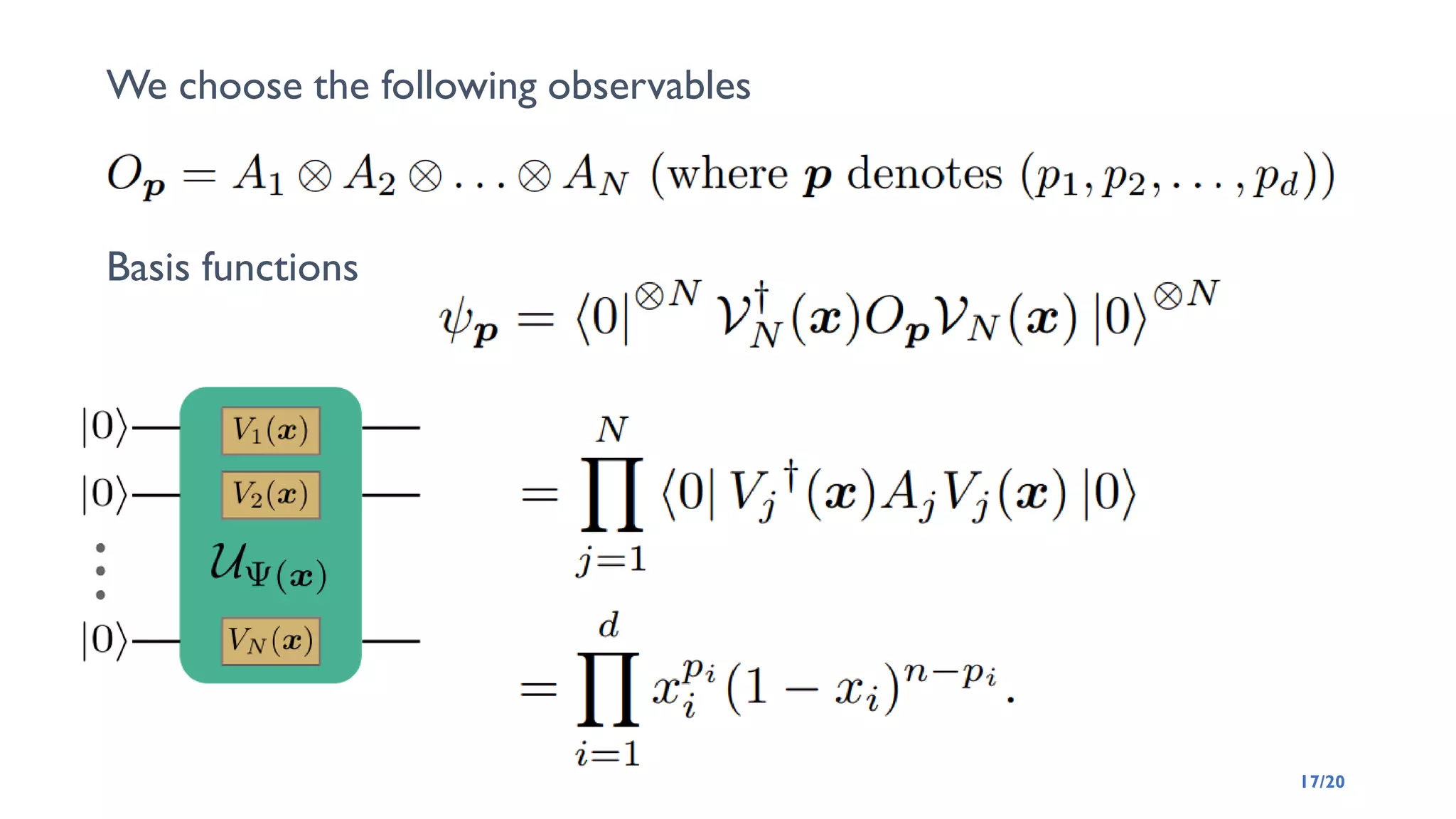
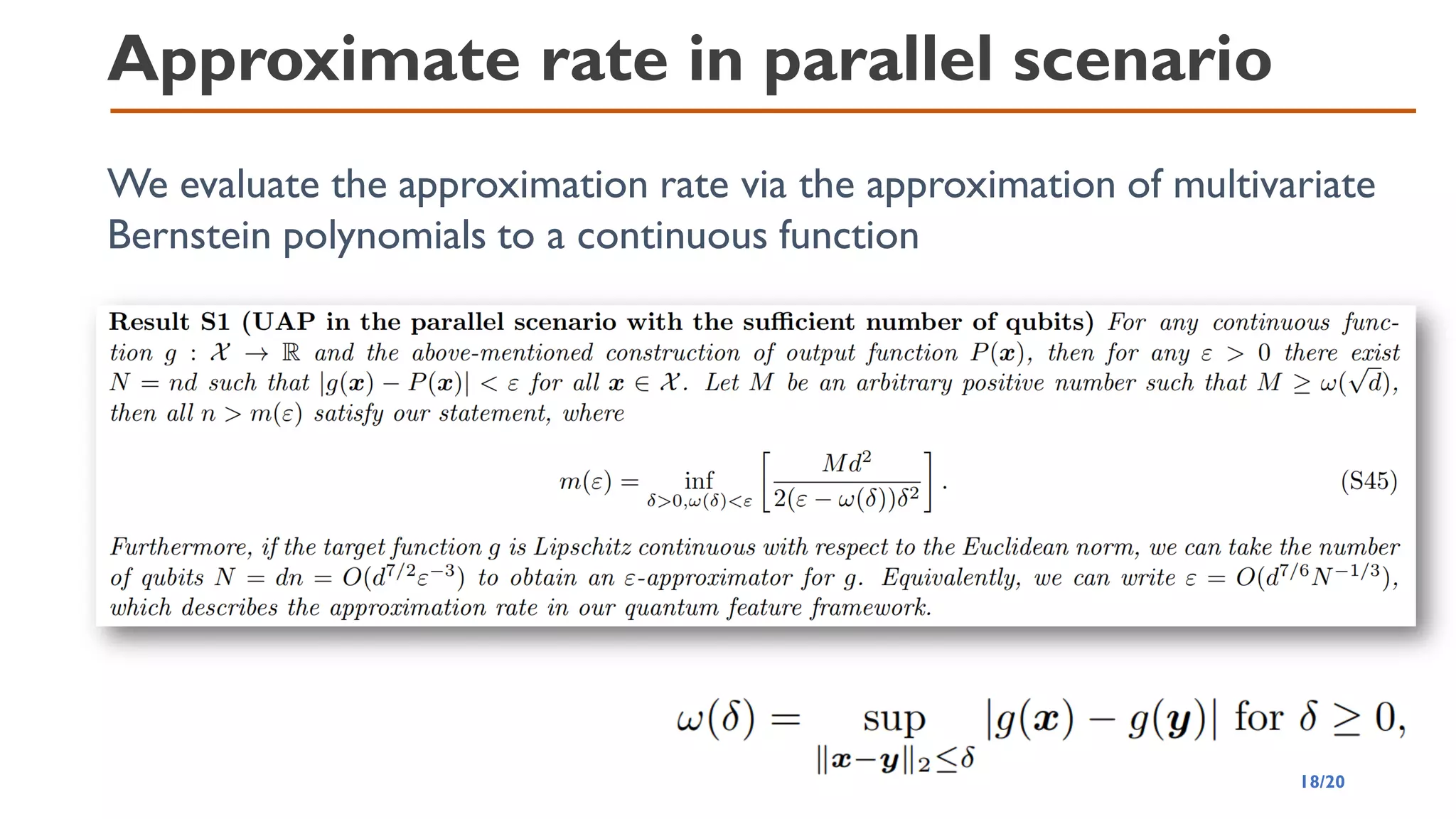
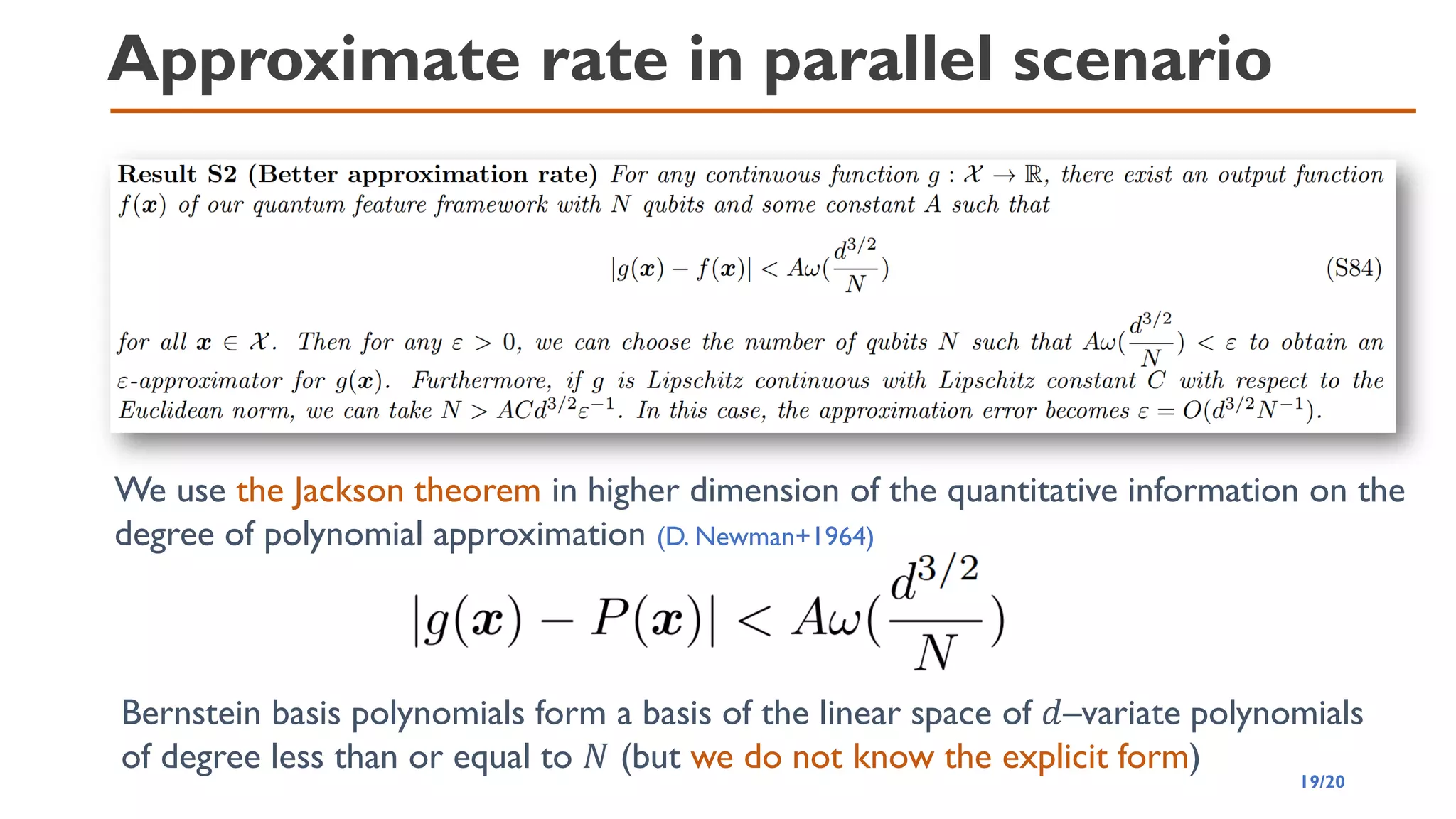
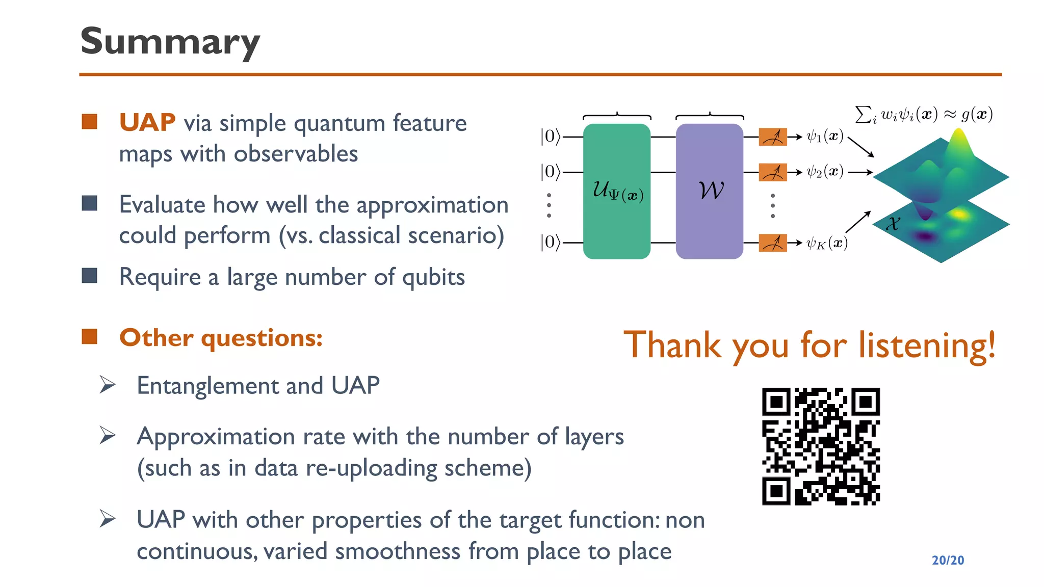

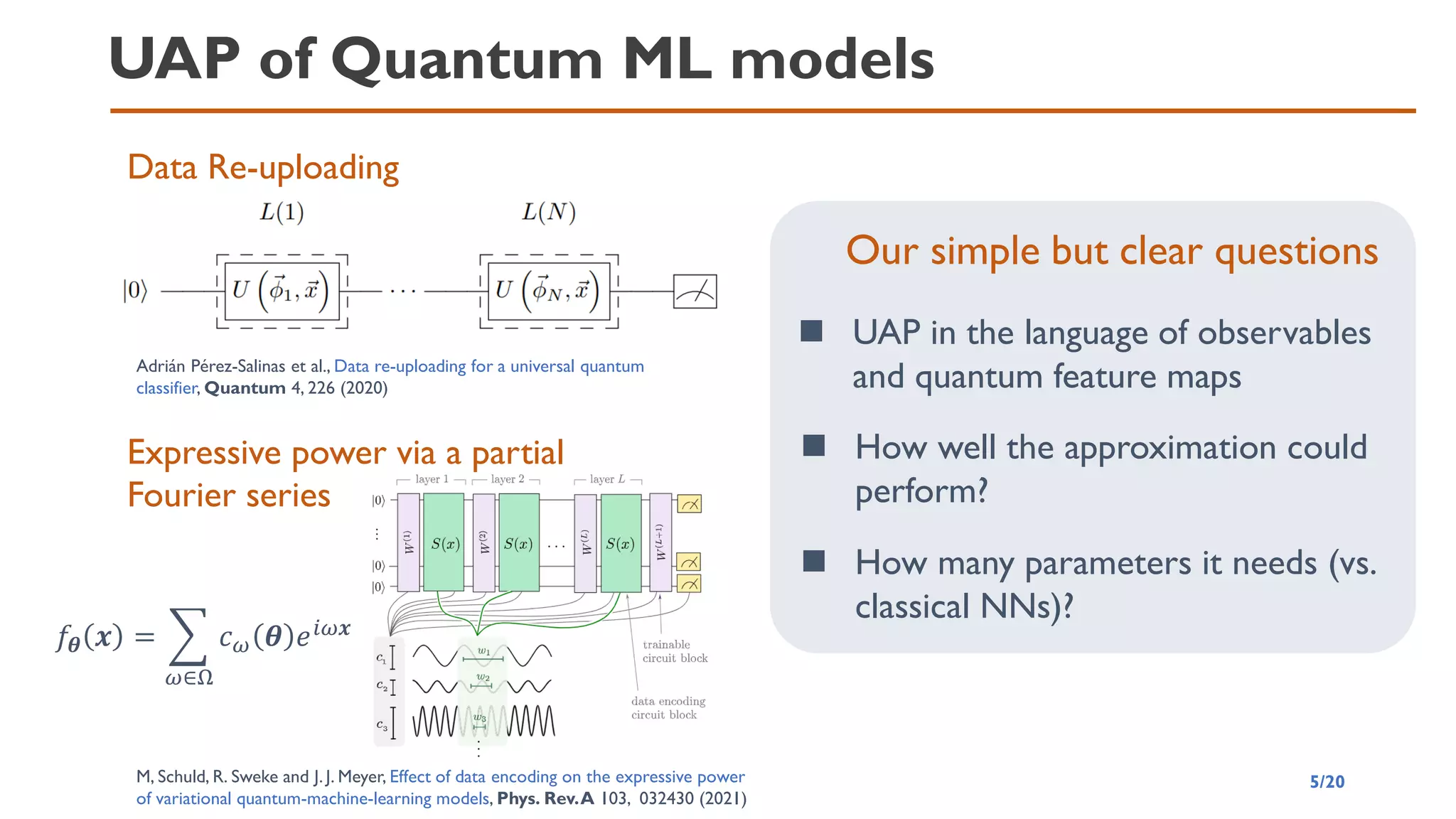
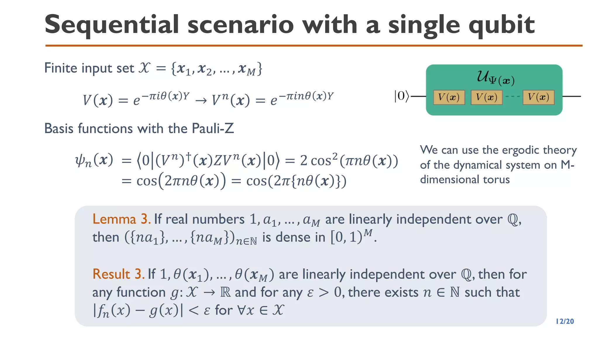
This document discusses the universal approximation property (UAP) of quantum neural networks (QNNs) using quantum feature maps, highlighting their potential advantages over classical neural networks. It explores the expressivity of QNNs, methods for achieving UAP through suitable observables and activation functions, and the implications of using quantum circuits for approximation. The authors suggest QNNs can approximate continuous functions effectively and pose various research questions related to approximation performance, entanglement, and the impact of network architecture.


