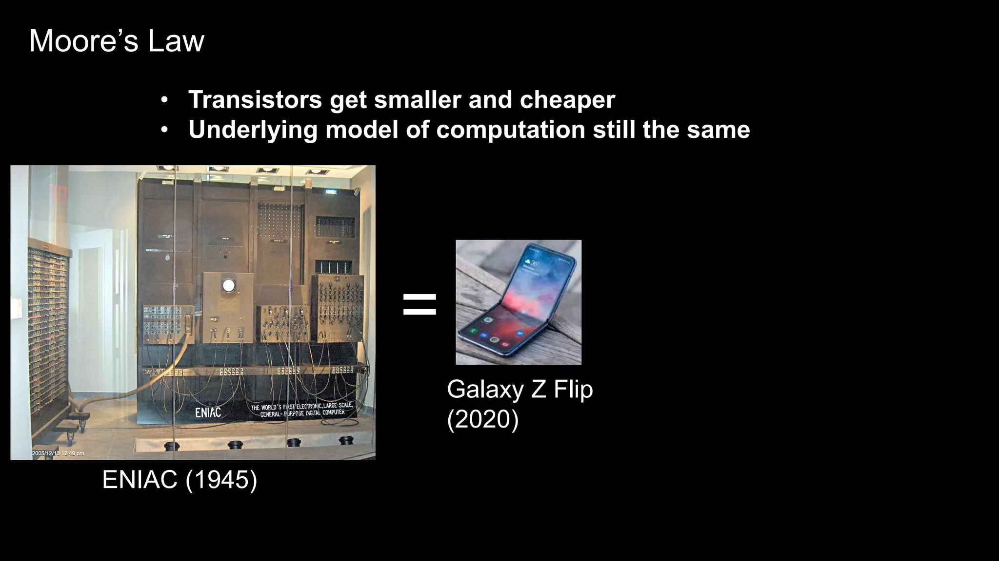
The document discusses quantum computing and IBM's efforts in the field. It provides an overview of quantum computing concepts like superposition and entanglement. It describes IBM's superconducting qubit technology and how qubits can be controlled and entangled. The document outlines IBM's quantum computing platforms including the IBM Quantum Experience for experimenting with quantum circuits in the cloud. It encourages users to get involved with the Qiskit open source framework and global quantum computing community.
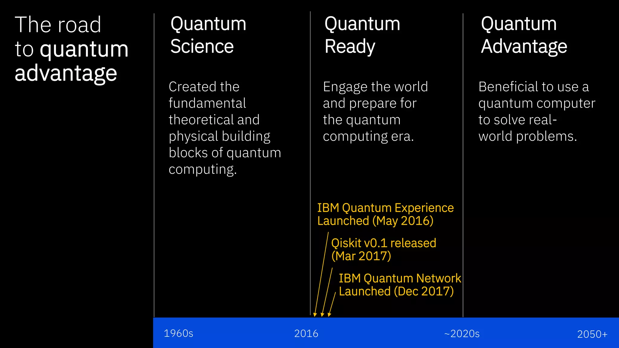
The road
to quantum
advantage
2016~2020s1960s 2050+
Quantum
Science
Quantum
Ready
Quantum
Advantage
Created the
fundamental
theoretical and
physical building
blocks of quantum
computing.
Engage the world
and prepare for
the quantum
computing era.
Beneficial to use a
quantum computer
to solve real-
world problems.
IBM Quantum Experience
Launched (May 2016)
IBM Quantum Network
Launched (Dec 2017)
Qiskit v0.1 released
(Mar 2017)
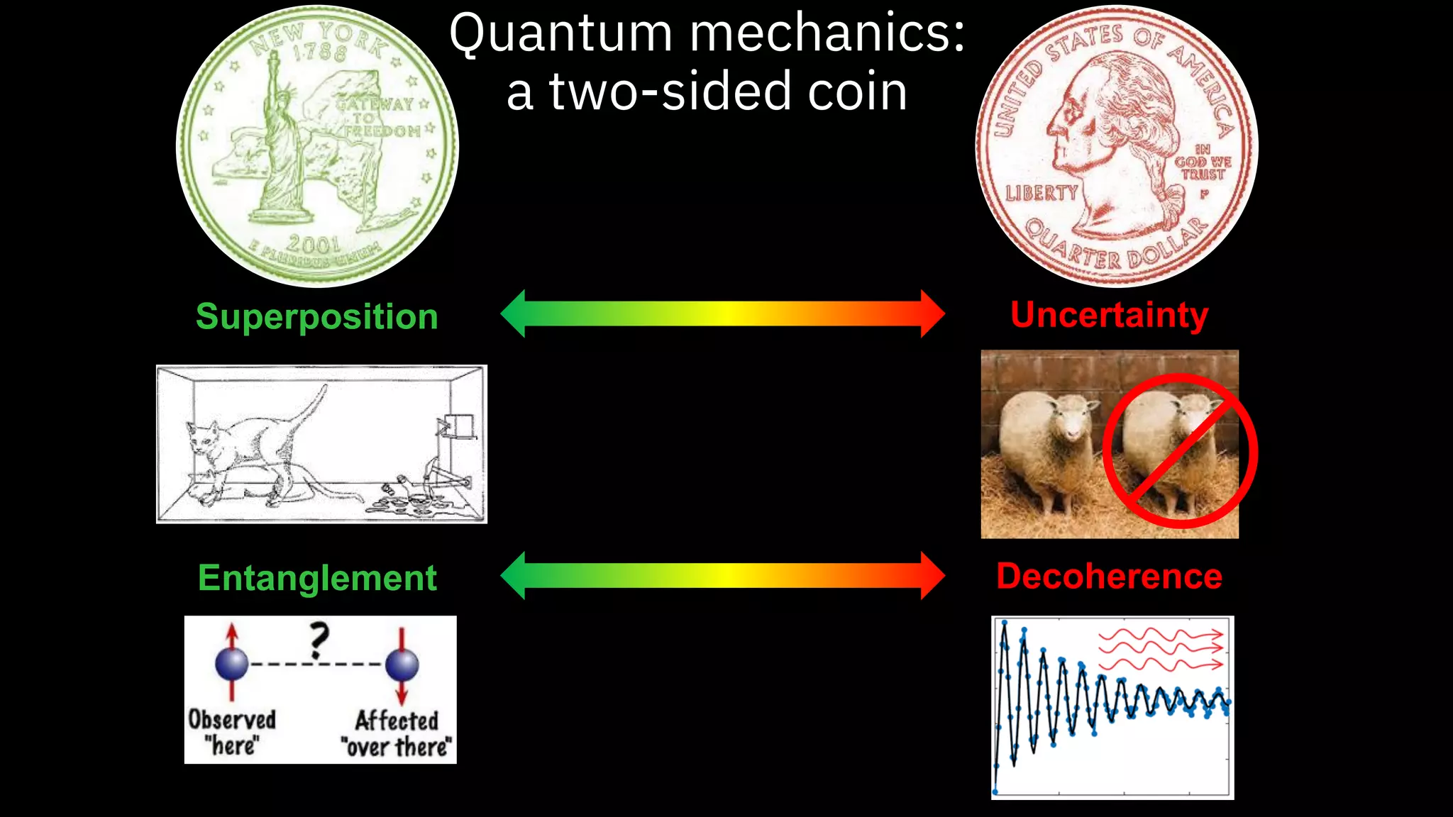
Computing with quantummechanics: features
Superposition: a system’s state can be any
linear combination of classical states …until
it is measured, at which point it collapses to
one of the classical states
Example: Schrodinger’s Cat
Entanglement: particles in superposition
can develop correlations such that
measuring just one affects them all
Example: EPR Paradox (Einstein: “spooky
action at a distance”)
Quantum
wavefunction
Normalization
“Classical” states
Linear
combination
9.
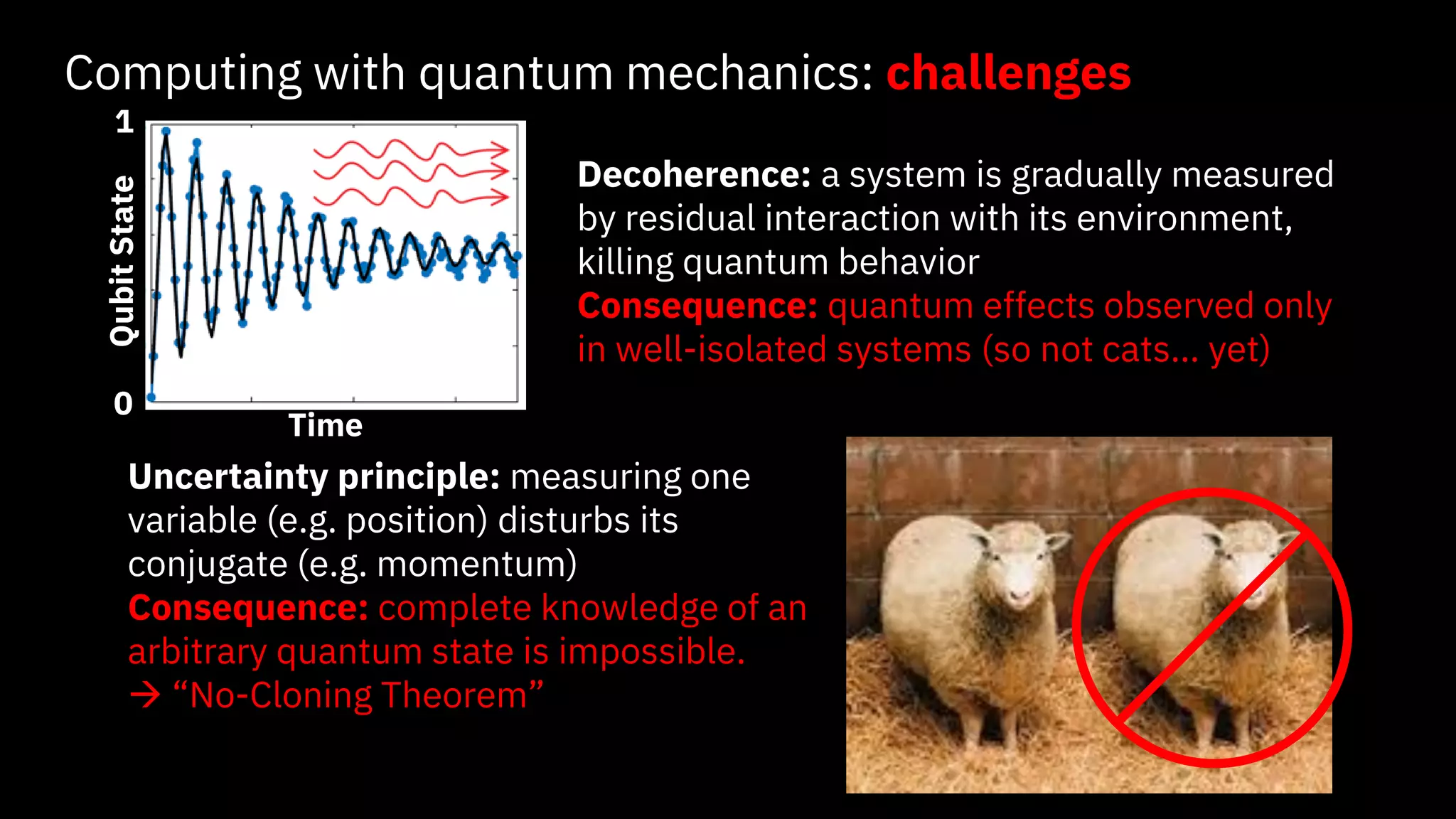
Computing with quantummechanics: challenges
Time
QubitState
0
1
Decoherence: a system is gradually measured
by residual interaction with its environment,
killing quantum behavior
Consequence: quantum effects observed only
in well-isolated systems (so not cats… yet)
Uncertainty principle: measuring one
variable (e.g. position) disturbs its
conjugate (e.g. momentum)
Consequence: complete knowledge of an
arbitrary quantum state is impossible.
→ “No-Cloning Theorem”
10.
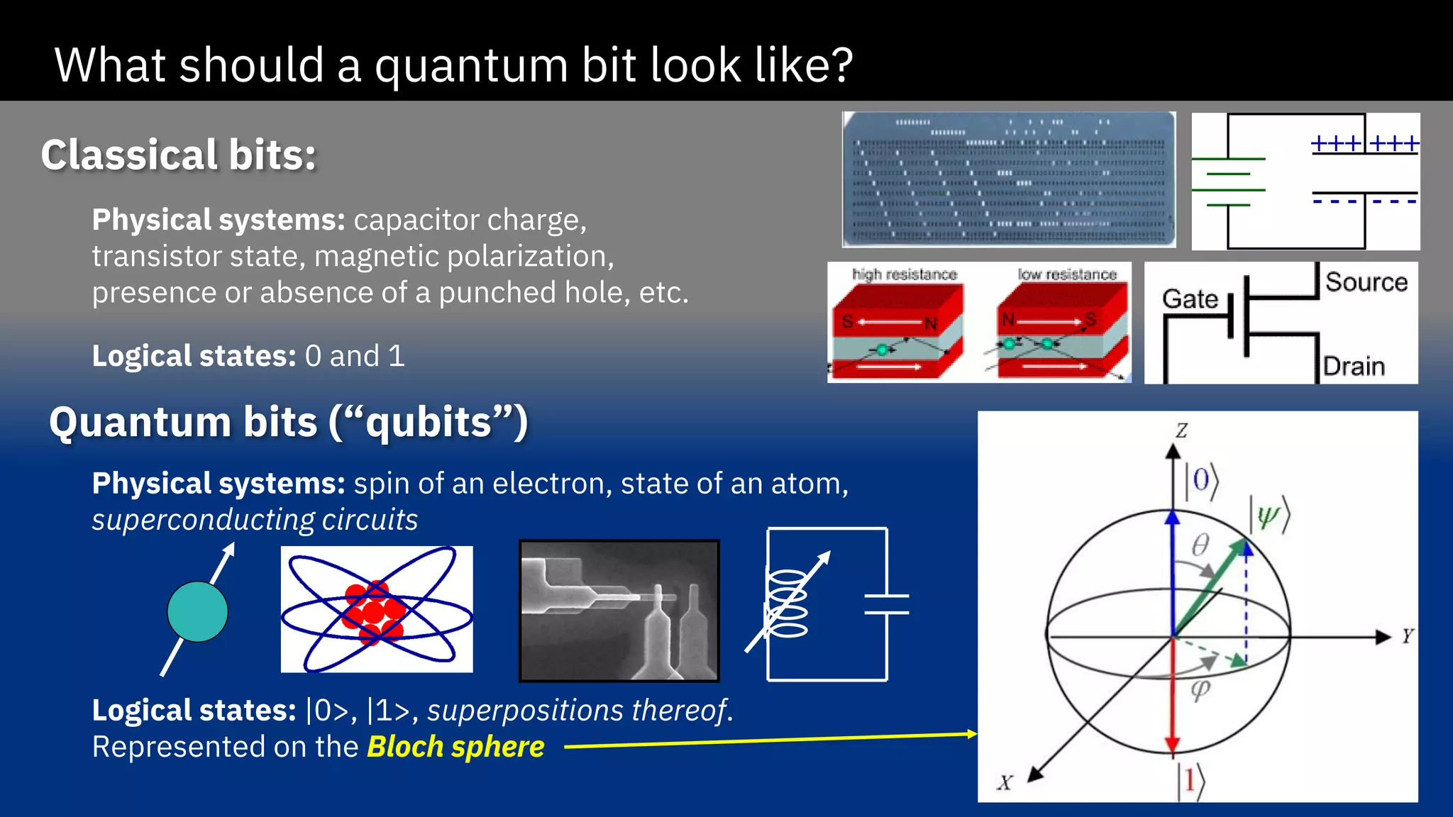
Classical bits:
Quantum bits(“qubits”)
What should a quantum bit look like?
Physical systems: capacitor charge,
transistor state, magnetic polarization,
presence or absence of a punched hole, etc.
Logical states: 0 and 1
Physical systems: spin of an electron, state of an atom,
superconducting circuits
Logical states: |0>, |1>, superpositions thereof.
Represented on the Bloch sphere
11.
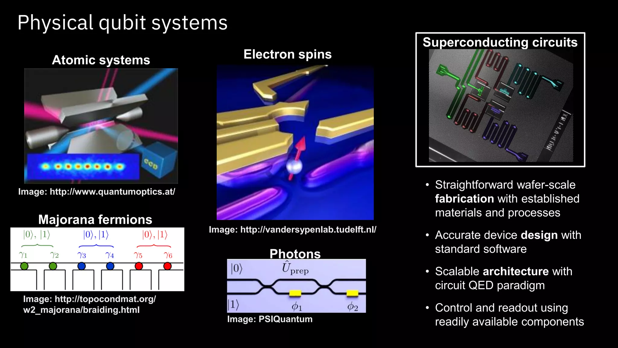
Physical qubit systems
Topological
systems?
Atomicsystems Electron spins
Image: http://vandersypenlab.tudelft.nl/
Image: http://www.quantumoptics.at/
Image: http://topocondmat.org/
w2_majorana/braiding.html
Majorana fermions
Superconducting circuits
• Straightforward wafer-scale
fabrication with established
materials and processes
• Accurate device design with
standard software
• Scalable architecture with
circuit QED paradigm
• Control and readout using
readily available components
Photons
Image: PSIQuantum
12.
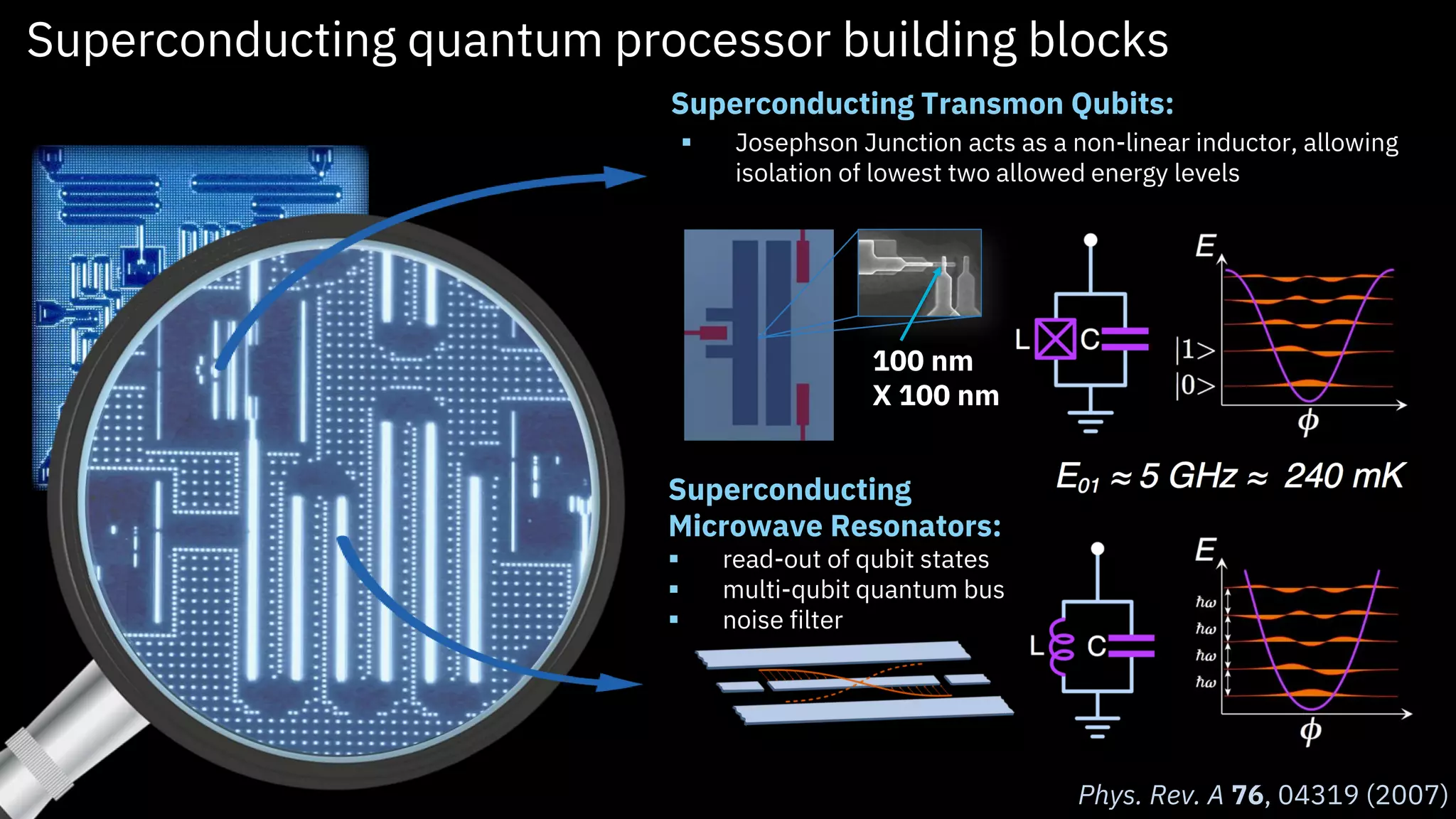
Superconducting
Microwave Resonators:
▪ read-outof qubit states
▪ multi-qubit quantum bus
▪ noise filter
Superconducting Transmon Qubits:
Superconducting quantum processor building blocks
100 nm
X 100 nm
▪ Josephson Junction acts as a non-linear inductor, allowing
isolation of lowest two allowed energy levels
Phys. Rev. A 76, 04319 (2007)
13.
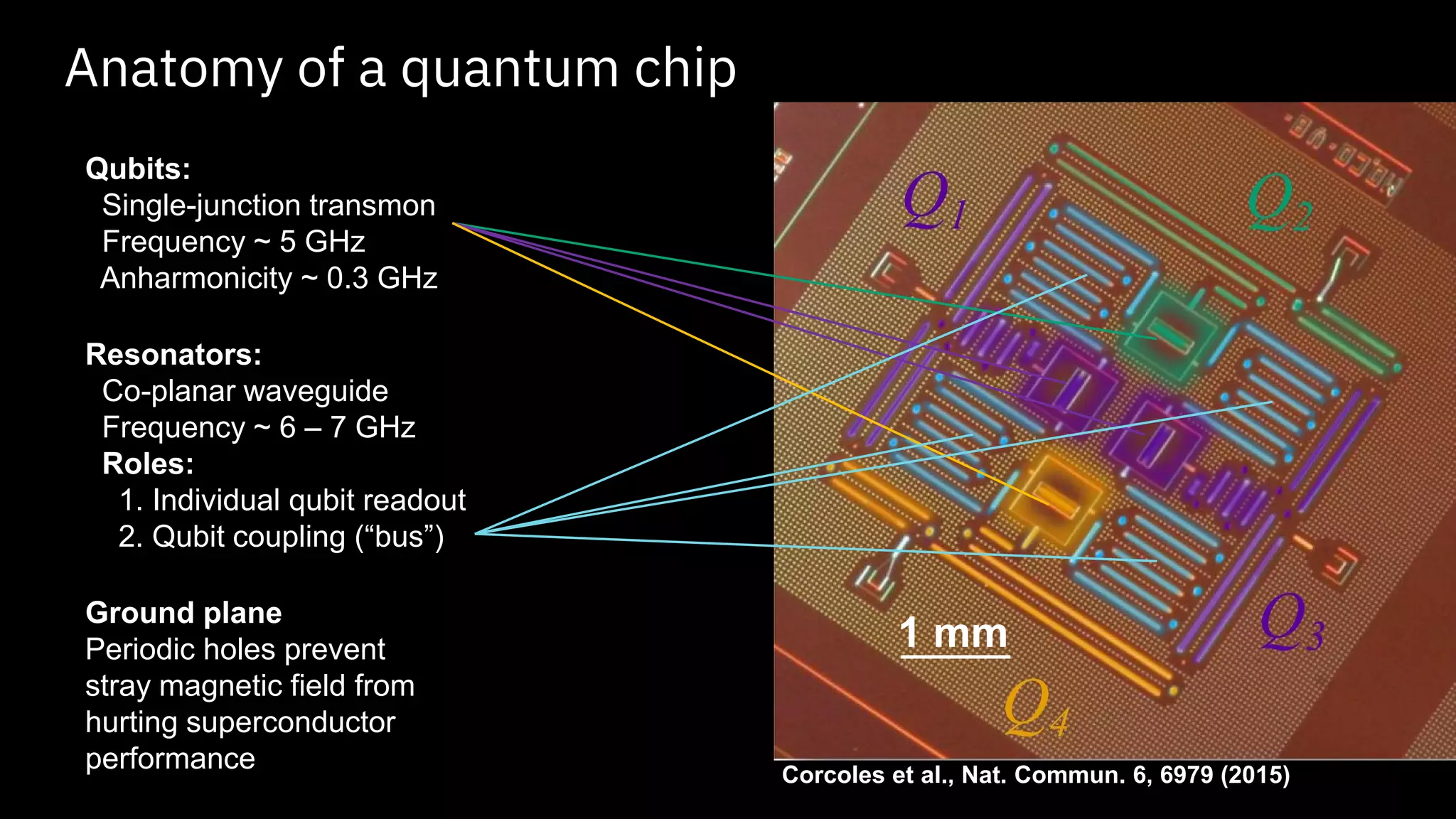
Anatomy of aquantum chip
1 mm
Qubits:
Single-junction transmon
Frequency ~ 5 GHz
Anharmonicity ~ 0.3 GHz
Resonators:
Co-planar waveguide
Frequency ~ 6 – 7 GHz
Roles:
1. Individual qubit readout
2. Qubit coupling (“bus”)
Ground plane
Periodic holes prevent
stray magnetic field from
hurting superconductor
performance Corcoles et al., Nat. Commun. 6, 6979 (2015)
14.
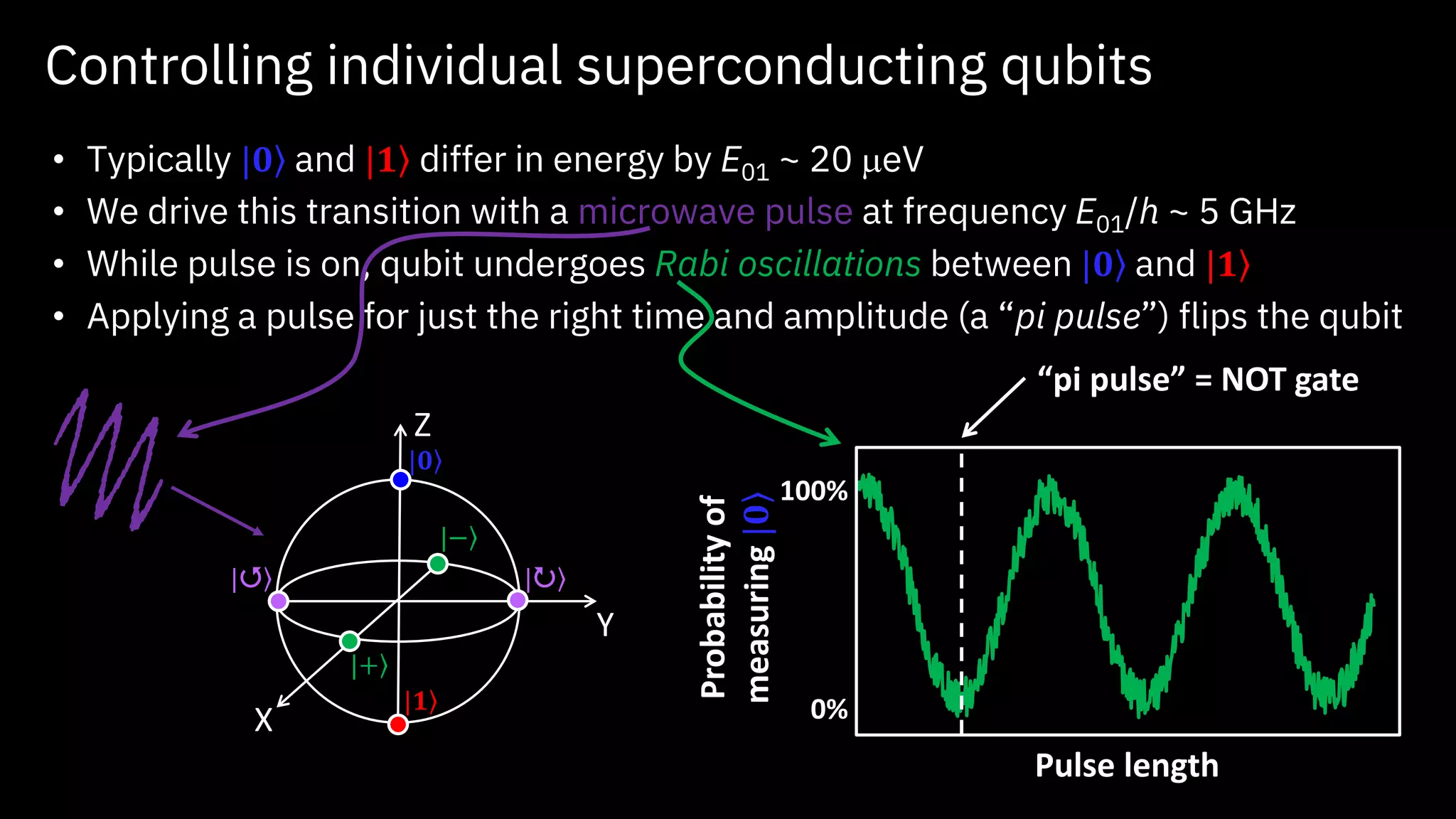
Controlling individual superconductingqubits
• Typically | ۧ𝟎 and | ۧ𝟏 differ in energy by E01 ~ 20 meV
• We drive this transition with a microwave pulse at frequency E01/h ~ 5 GHz
• While pulse is on, qubit undergoes Rabi oscillations between | ۧ𝟎 and | ۧ𝟏
• Applying a pulse for just the right time and amplitude (a “pi pulse”) flips the qubit
X
Y
Z
| ۧ𝟎
| ۧ𝟏
| ۧ+
| ۧ−
| ۧ| ۧ
Pulse length
Probabilityof
measuring|ۧ𝟎
100%
0%
“pi pulse” = NOT gate
15.
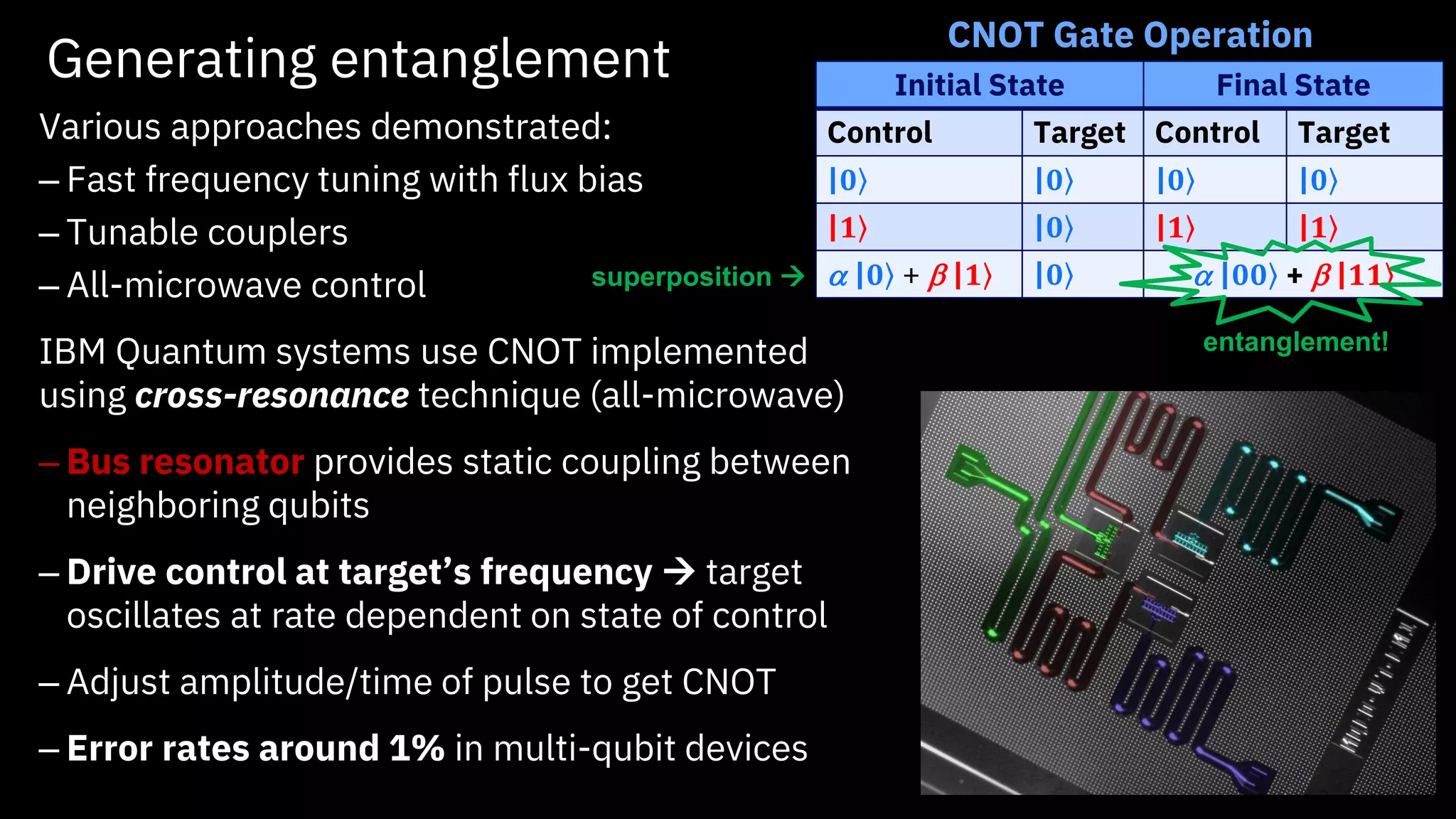
Generating entanglement
Various approachesdemonstrated:
– Fast frequency tuning with flux bias
– Tunable couplers
– All-microwave control
IBM Quantum systems use CNOT implemented
using cross-resonance technique (all-microwave)
– Bus resonator provides static coupling between
neighboring qubits
– Drive control at target’s frequency → target
oscillates at rate dependent on state of control
– Adjust amplitude/time of pulse to get CNOT
– Error rates around 1% in multi-qubit devices
Initial State Final State
Control Target Control Target
| ۧ𝟎 | ۧ𝟎 | ۧ𝟎 | ۧ𝟎
| ۧ𝟏 | ۧ𝟎 | ۧ𝟏 | ۧ𝟏
a | ۧ𝟎 + b | ۧ𝟏 | ۧ𝟎 a | ۧ𝟎𝟎 + b | ۧ𝟏𝟏
CNOT Gate Operation
entanglement!
superposition →
16.
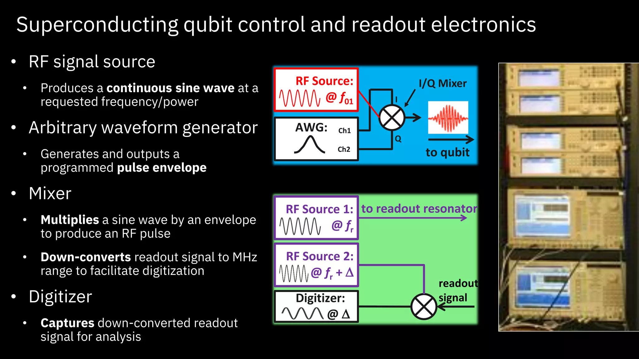
Superconducting qubit controland readout electronics
• RF signal source
• Produces a continuous sine wave at a
requested frequency/power
• Arbitrary waveform generator
• Generates and outputs a
programmed pulse envelope
• Mixer
• Multiplies a sine wave by an envelope
to produce an RF pulse
• Down-converts readout signal to MHz
range to facilitate digitization
• Digitizer
• Captures down-converted readout
signal for analysis
RF Source:
@ f01
AWG: Ch1
Ch2
I
Q
to qubit
I/Q Mixer
Qubit control:
RF Source 1:
@ fr
Digitizer:
@ D
to readout resonator
Qubit readout:
RF Source 2:
@ fr + D
readout
signal
17.
Superconducting qubit environmentand signal flow
• Cryo temperatures required
▪ Qubits sit at base of dilution refrigerator
• Control and readout performed by
sending pulses over coaxial cables
• Input lines use attenuation to
reduce incoming noise
• Output lines use cryogenic
amplification and isolation
18.
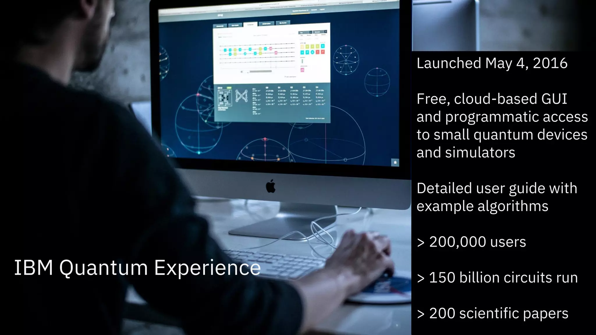
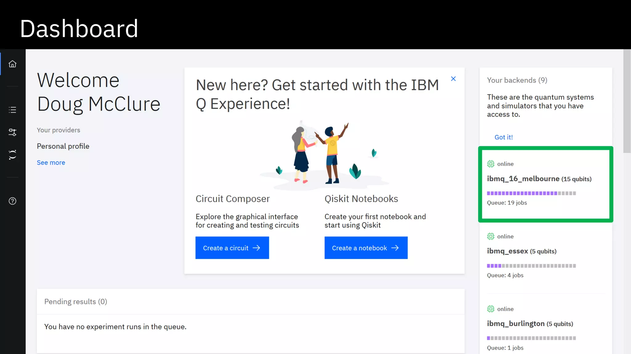
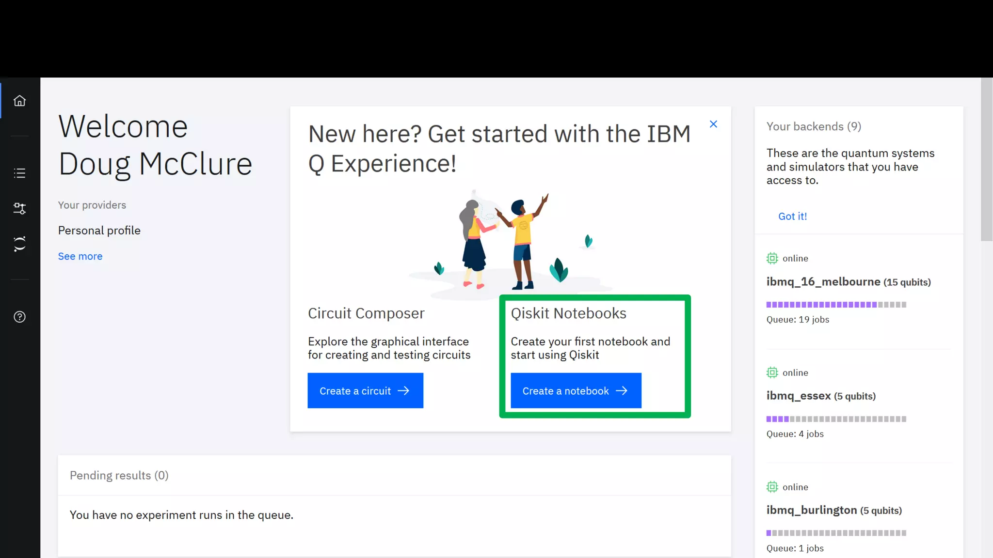
IBM Quantum Experience
LaunchedMay 4, 2016
Free, cloud-based GUI
and programmatic access
to small quantum devices
and simulators
Detailed user guide with
example algorithms
> 200,000 users
> 150 billion circuits run
> 200 scientific papers
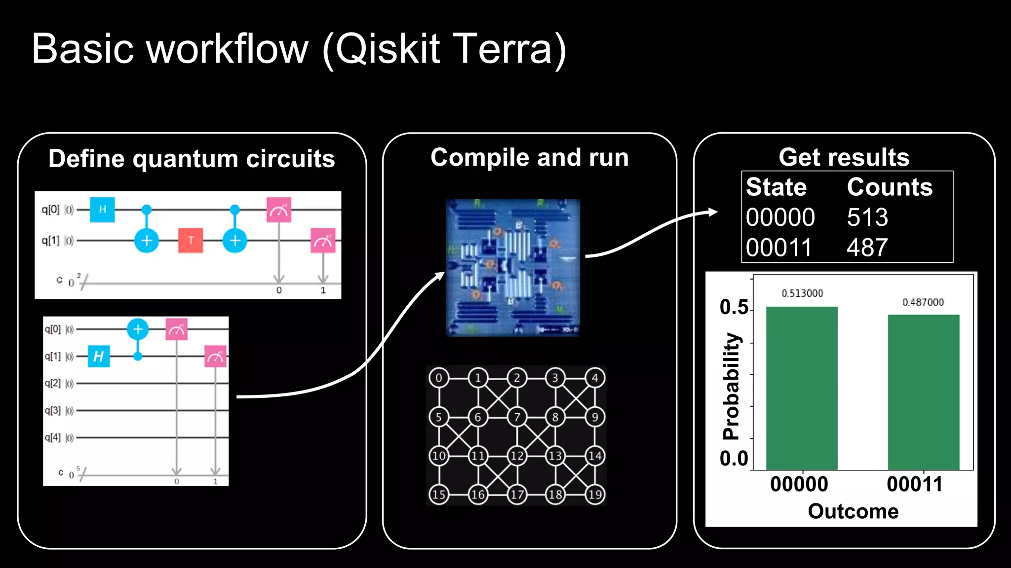
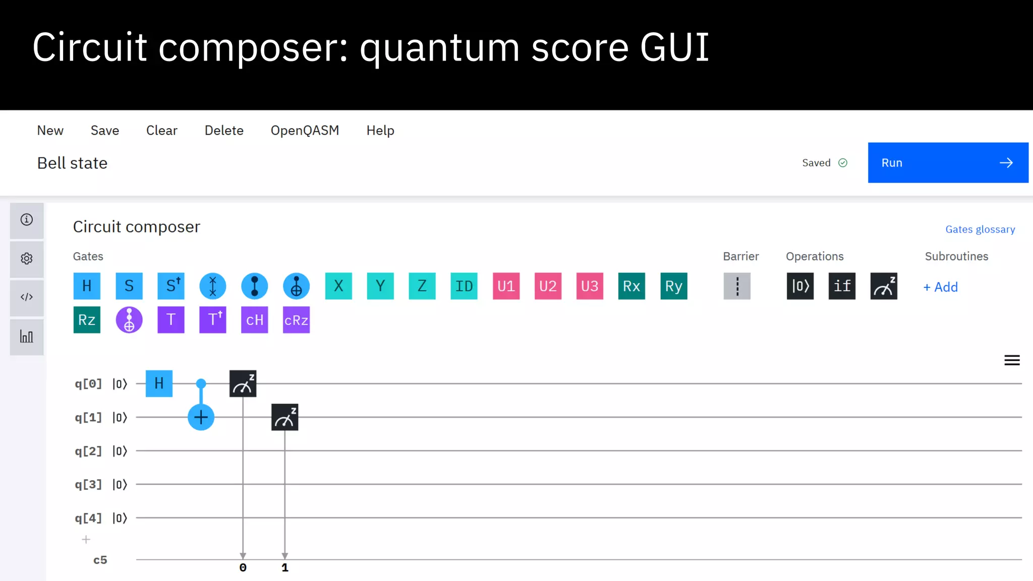
Writing quantum circuits:the “quantum score”
arxiv.org/pdf/1905.02666.pdf
• “Textbook” way of showing quantum circuits
• Conducive to user-friendly drag-and-drop interface
• Useful for beginners studying simple circuits
• Becomes unmanageable for large/complex circuits
21.
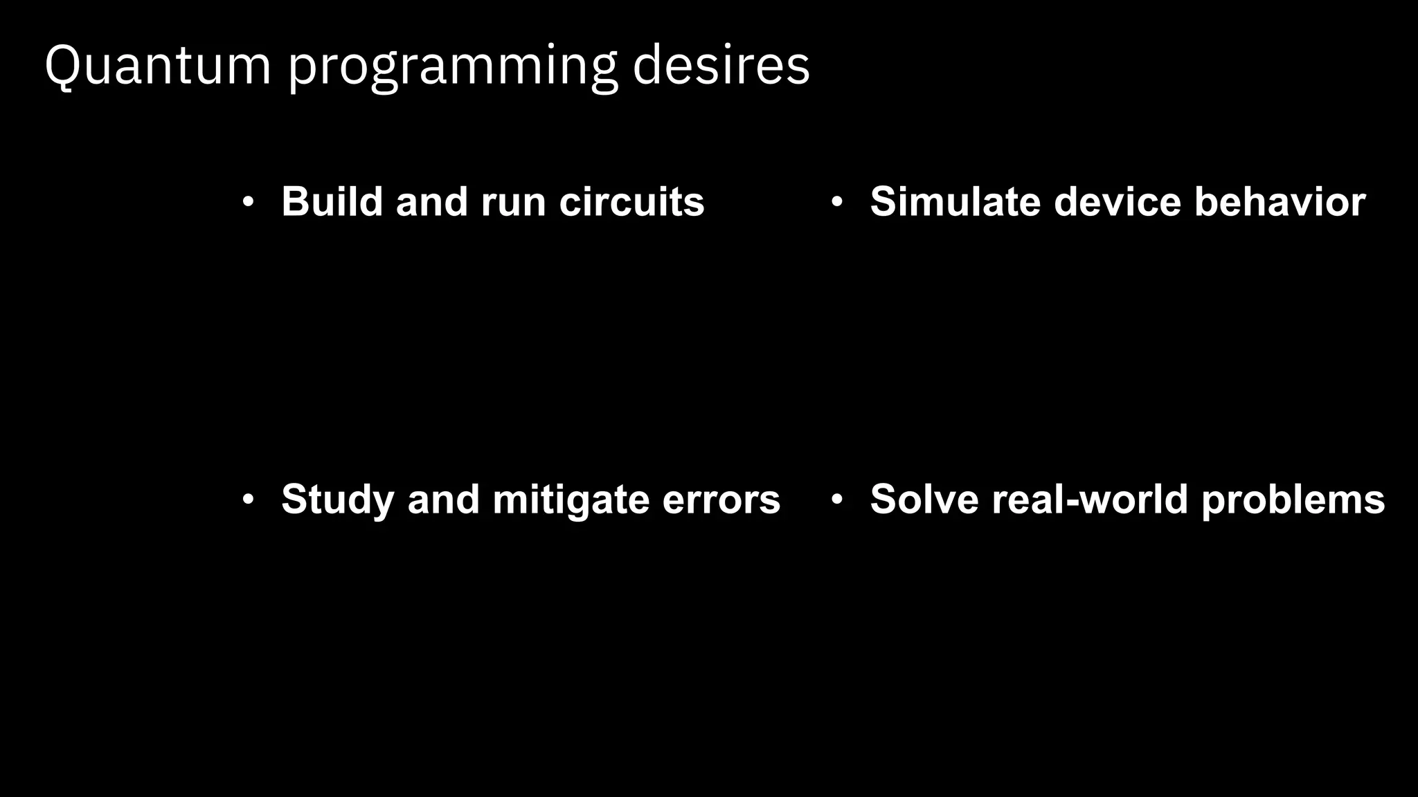
Quantum programming desires
•Build and run circuits
• Study and mitigate errors
• Simulate device behavior
• Solve real-world problems
22.
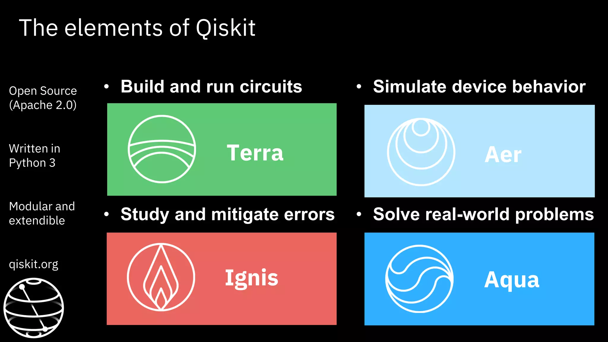
The elements ofQiskit
• Build and run circuits
• Study and mitigate errors
• Simulate device behavior
• Solve real-world problems
Terra
Aqua
Aer
Ignis
Open Source
(Apache 2.0)
Written in
Python 3
Modular and
extendible
qiskit.org
Designing algorithms fortoday’s quantum computers
• Quantum processors are noisy → long circuits won’t work!
▪ Design algorithms to use many small circuits rather than a single big one
• Example: “hybrid” quantum-classical optimization
▪ Quantum processor calculates objective function for classical optimizer
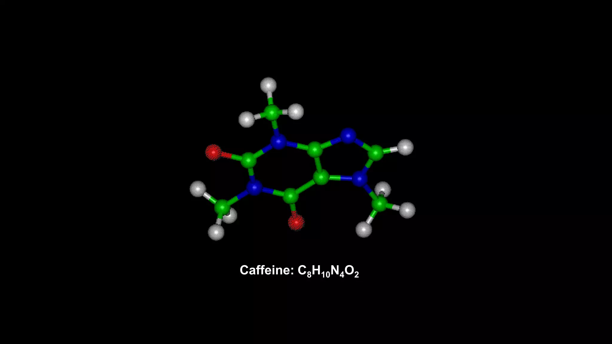
▪ Applicable to many problems including quantum chemistry (below)
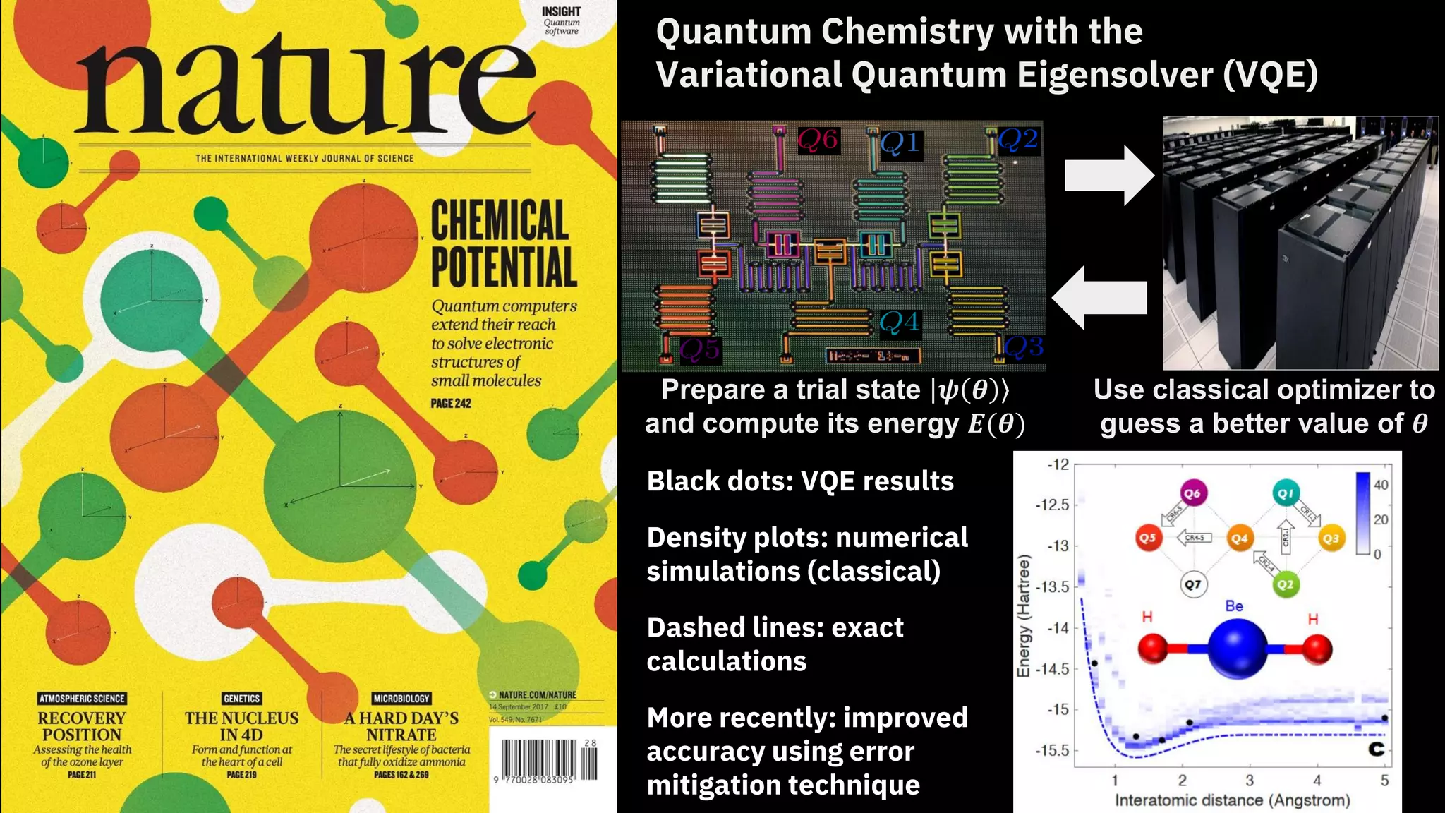
Prepare a trial state 𝝍 𝜽
and compute its energy 𝑬(𝜽)
Use classical optimizer to
guess a better value of 𝜽
25.
Black dots: VQEresults
Density plots: numerical
simulations (classical)
Dashed lines: exact
calculations
More recently: improved
accuracy using error
mitigation technique
Prepare a trial state 𝝍 𝜽
and compute its energy 𝑬(𝜽)
Use classical optimizer to
guess a better value of 𝜽
Quantum Chemistry with the
Variational Quantum Eigensolver (VQE)
26.
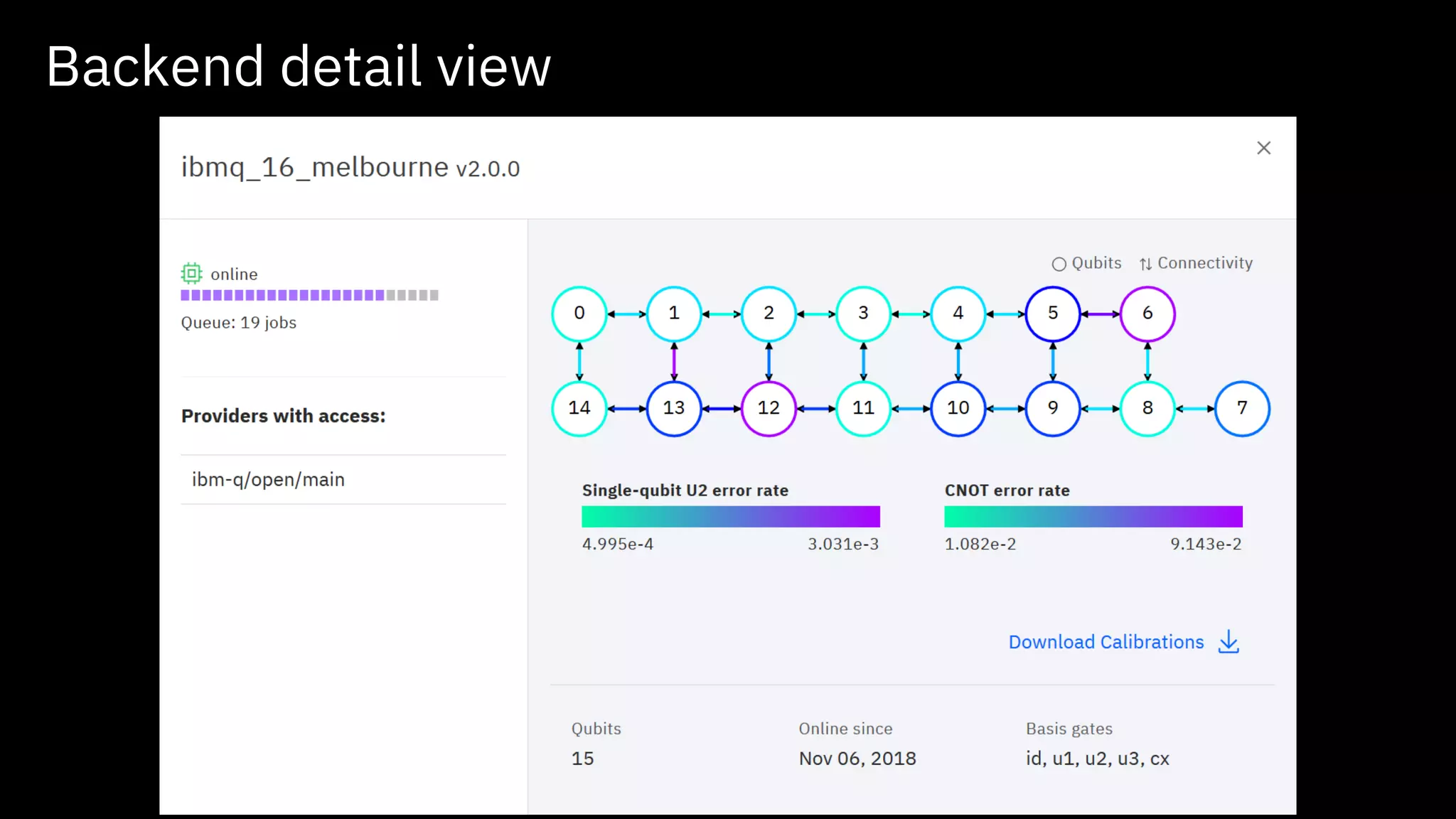
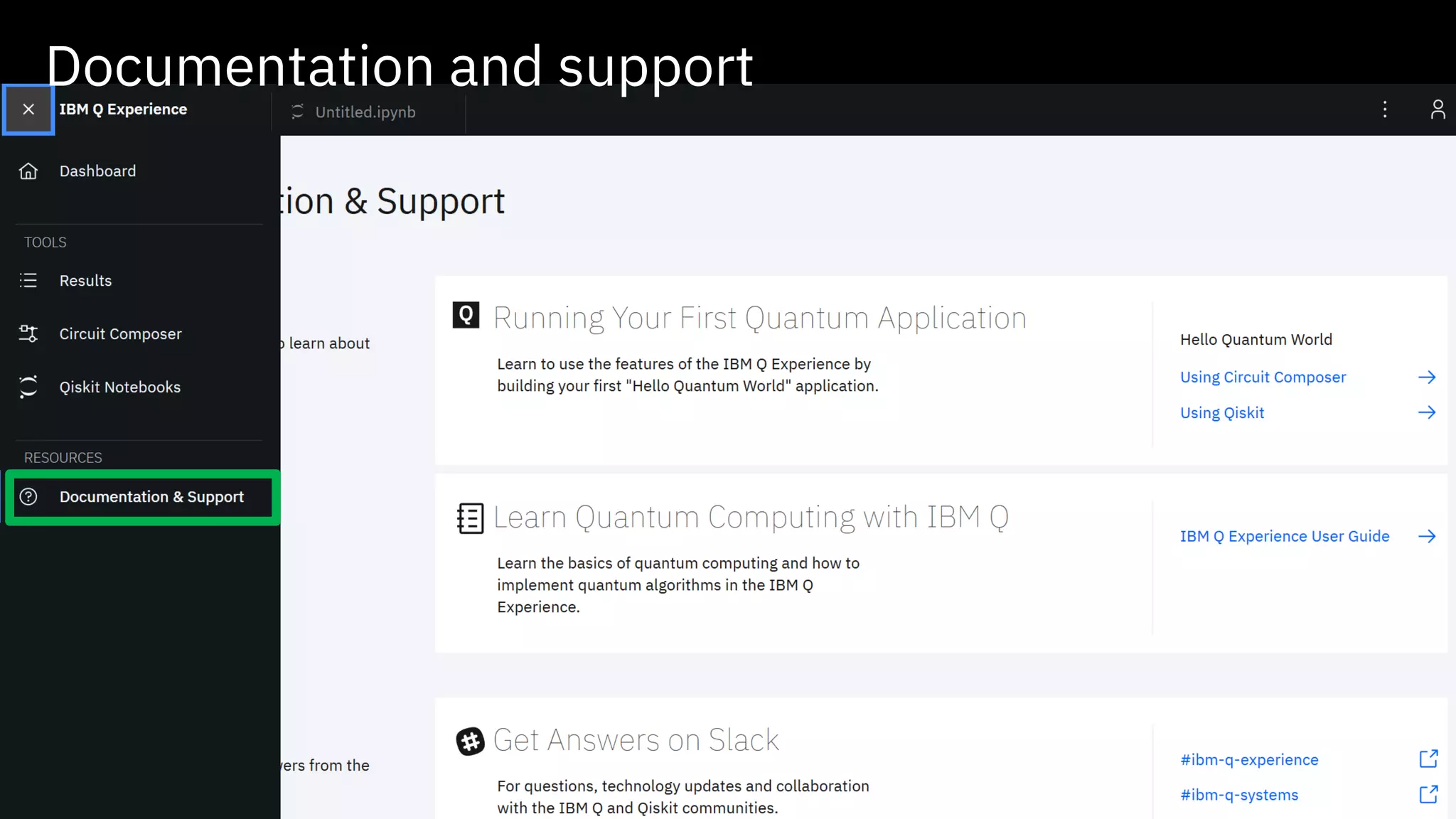
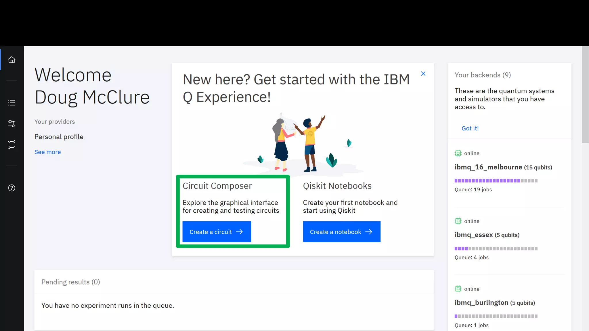
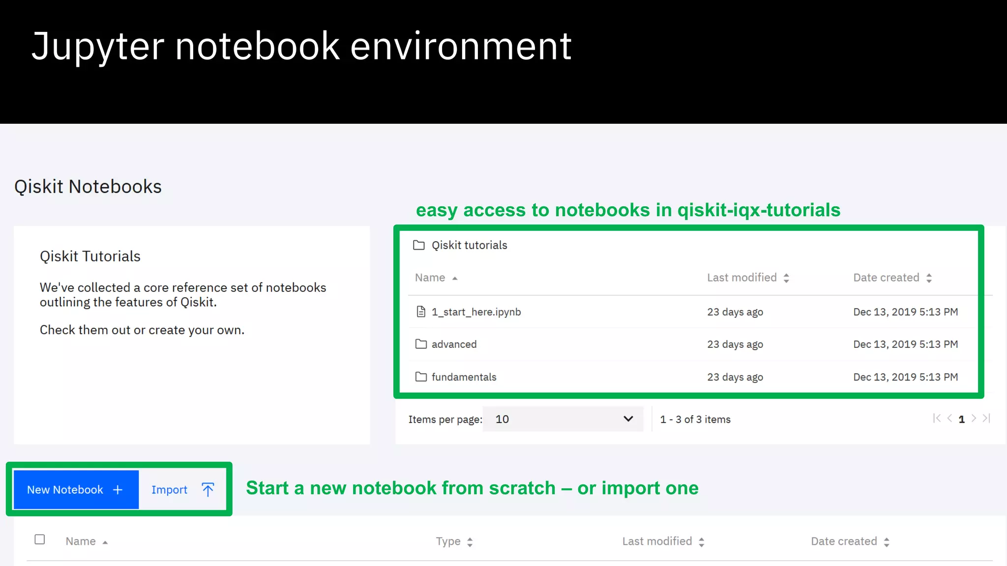
Tour of IQXPlatform
arxiv.org/pdf/1905.02666.pdf
quantum-computing.ibm.com
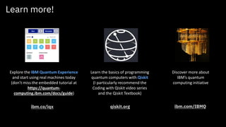
Learn more!
Discover moreabout
IBM’s quantum
computing initiative
ibm.com/IBMQ
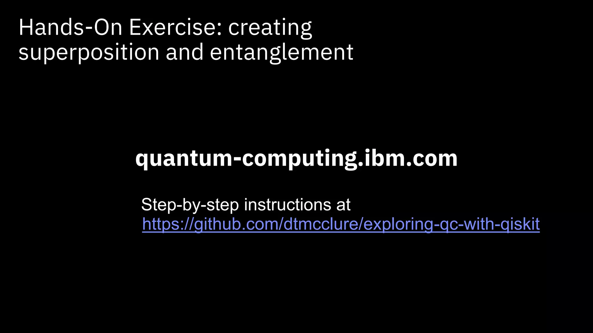
Explore the IBM Quantum Experience
and start using real machines today
(don’t miss the embedded tutorial at
https://quantum-
computing.ibm.com/docs/guide)
ibm.co/iqx
Learn the basics of programming
quantum computers with Qiskit
(I particularly recommend the
Coding with Qiskit video series
and the Qiskit Textbook)
qiskit.org