Downloaded 313 times
![#FaithFUL Dataset 1D
#
#load data
#
data(faithful)
Y<-faithful$waiting
#
#plot histogram of waiting times
#
postscript("geyser.eps",width=5,height=3,onefile=F)
par(mar=c(2,2,1,1),mgp=c(1,0.5,0),cex=0.7,lwd=0.5,las=1)
hist(Y,breaks=seq(40,100,3),xlab="Waiting time between eruptions (min)",
xlim=c(40,100),main="",axes=F)
axis(1,seq(40,100,6),pos=0)
axis(2,seq(0,35,5),pos=40,las=1)
dev.off()
#
#log-likelihood function
#
ln<-function(p,Y) {
-sum(log(p[1]*dnorm(Y,p[2],sqrt(p[4]))+(1-p[1])*dnorm(Y,p[3],sqrt(p[5]))))
}
#
#EM algorithm
#
emstep<-function(Y,p) {
EZ<-p[1]*dnorm(Y,p[2],sqrt(p[4]))/
(p[1]*dnorm(Y,p[2],sqrt(p[4]))
+(1-p[1])*dnorm(Y,p[3],sqrt(p[5])))
p[1]<-mean(EZ)
p[2]<-sum(EZ*Y)/sum(EZ)
p[3]<-sum((1-EZ)*Y)/sum(1-EZ)
p[4]<-sum(EZ*(Y-p[2])^2)/sum(EZ)
p[5]<-sum((1-EZ)*(Y-p[3])^2)/sum(1-EZ)
p
}
emiteration<-function(Y,p,n=10) {
for (i in (1:n)) {
p<-emstep(Y,p)
}
p
}
#
#starting values
#
p<-c(0.5,40,90,16,16)
#
#2 iterations of EM algorithm
#
p<-emiteration(Y,p,2)
p
#check for convergence
p<-emstep(Y,p)
p
#
#plot histogram with fitted distribution
#
hist(Y,breaks=seq(40,100,3),xlab="Waiting time between eruptions (min)",
xlim=c(40,100),
main="",axes=F)
axis(1,seq(40,100,6),pos=0)](https://image.slidesharecdn.com/rcodeforemalgorithm-160506141904/85/R-Code-for-EM-Algorithm-3-320.jpg)
![axis(2,seq(0,35,5),pos=40,las=1)
x<-seq(40,100,0.1)
y<-p[1]*dnorm(x,p[2],sqrt(p[4]))+(1-p[1])*dnorm(x,p[3],sqrt(p[5]))
lines(x,y*3*length(Y))
#5 iterations of EM algorithm
#log-likelihood function
#
ln<-function(p,Y) {
-sum(log(p[1]*dnorm(Y,p[2],sqrt(p[4]))+(1-p[1])*dnorm(Y,p[3],sqrt(p[5]))))
}
#
#EM algorithm
#
emstep<-function(Y,p) {
EZ<-p[1]*dnorm(Y,p[2],sqrt(p[4]))/
(p[1]*dnorm(Y,p[2],sqrt(p[4]))
+(1-p[1])*dnorm(Y,p[3],sqrt(p[5])))
p[1]<-mean(EZ)
p[2]<-sum(EZ*Y)/sum(EZ)
p[3]<-sum((1-EZ)*Y)/sum(1-EZ)
p[4]<-sum(EZ*(Y-p[2])^2)/sum(EZ)
p[5]<-sum((1-EZ)*(Y-p[3])^2)/sum(1-EZ)
p
}
emiteration<-function(Y,p,n=10) {
for (i in (1:n)) {
p<-emstep(Y,p)
}
p
}
#
#starting values
#
p<-c(0.5,40,90,16,16)
#
#5 iterations of EM algorithm
#
p<-emiteration(Y,p,5)
p
#check for convergence
p<-emstep(Y,p)
p
#
#plot histogram with fitted distribution
#
hist(Y,breaks=seq(40,100,3),xlab="Waiting time between eruptions (min)",
xlim=c(40,100),
main="",axes=F)
axis(1,seq(40,100,6),pos=0)
axis(2,seq(0,35,5),pos=40,las=1)
x<-seq(40,100,0.1)
y<-p[1]*dnorm(x,p[2],sqrt(p[4]))+(1-p[1])*dnorm(x,p[3],sqrt(p[5]))
lines(x,y*3*length(Y))
#10 iterations of EM algorithm
#log-likelihood function
#
ln<-function(p,Y) {
-sum(log(p[1]*dnorm(Y,p[2],sqrt(p[4]))+(1-p[1])*dnorm(Y,p[3],sqrt(p[5]))))
}
#
#EM algorithm
#
emstep<-function(Y,p) {
EZ<-p[1]*dnorm(Y,p[2],sqrt(p[4]))/
(p[1]*dnorm(Y,p[2],sqrt(p[4]))
+(1-p[1])*dnorm(Y,p[3],sqrt(p[5])))](https://image.slidesharecdn.com/rcodeforemalgorithm-160506141904/85/R-Code-for-EM-Algorithm-4-320.jpg)
![p[1]<-mean(EZ)
p[2]<-sum(EZ*Y)/sum(EZ)
p[3]<-sum((1-EZ)*Y)/sum(1-EZ)
p[4]<-sum(EZ*(Y-p[2])^2)/sum(EZ)
p[5]<-sum((1-EZ)*(Y-p[3])^2)/sum(1-EZ)
p
}
emiteration<-function(Y,p,n=10) {
for (i in (1:n)) {
p<-emstep(Y,p)
}
p
}
#
#starting values
#
p<-c(0.5,40,90,16,16)
#
#10 iterations of EM algorithm
#
p<-emiteration(Y,p,10)
p
#check for convergence
p<-emstep(Y,p)
p
#
#plot histogram with fitted distribution
#
hist(Y,breaks=seq(40,100,3),xlab="Waiting time between eruptions (min)",
xlim=c(40,100),
main="",axes=F)
axis(1,seq(40,100,6),pos=0)
axis(2,seq(0,35,5),pos=40,las=1)
x<-seq(40,100,0.1)
y<-p[1]*dnorm(x,p[2],sqrt(p[4]))+(1-p[1])*dnorm(x,p[3],sqrt(p[5]))
lines(x,y*3*length(Y))
#Faithful Dataset 2D
#load data
#
#
#Bivariate mixture model
#
data(faithful)
Y<-faithful$waiting
X<-faithful$eruptions
plot(Y,X,xlab="Waiting time between eruptions (min)",
ylab="Eruption times (min)",
xlim=c(40,100),ylim=c(0,6),
main="",axes=F,cex=0.7)
axis(1,seq(40,100,6),pos=0)
axis(2,seq(0,6,1),pos=40,las=1)
#
#density of bivariate normal
#
dbinorm<-function(x,m,s){
1/sqrt(det(2*pi*s))*exp(-0.5*t(x-m)%*%solve(s)%*%(x-m))
}
f.hat<-function(x,p) {
p$p*dbinorm(x,p$m1,p$s1)+(1-p$p)*dbinorm(x,p$m2,p$s2)
}
Estep<-function(x,p) {
p$p*dbinorm(x,p$m1,p$s1)/](https://image.slidesharecdn.com/rcodeforemalgorithm-160506141904/85/R-Code-for-EM-Algorithm-5-320.jpg)
![(p$p*dbinorm(x,p$m1,p$s1)
+(1-p$p)*dbinorm(x,p$m2,p$s2))
}
emstep<-function(Y,p) {
EZ<-apply(Y,1,Estep,p)
p$p<-mean(EZ)
p$m1<-(t(Y)%*%diag(EZ)%*%rep(1,nrow(Y)))/sum(EZ)
p$m2<-(t(Y)%*%diag(1-EZ)%*%rep(1,nrow(Y)))/sum(1-EZ)
MY<-matrix(p$m1,nrow(Y),2,byrow=T)
p$s1<-(t(Y-MY)%*%diag(EZ)%*%(Y-MY))/sum(EZ)
MY<-matrix(p$m2,nrow(Y),2,byrow=T)
p$s2<-(t(Y-MY)%*%diag(1-EZ)%*%(Y-MY))/sum(1-EZ)
p
}
#----------------------------------
X<-faithful$waiting
Y<-faithful$eruptions
Z<-cbind(X,Y)
#starting values
#
p=p.0<-list(p=0.5,m1=c(20,6),m2=c(70,6),
s1=matrix(c(10,0,0,1),2,2),s2=matrix(c(10,0,0,1),2,2))
#--------------------------------------
lh=NULL
P=matrix(0,20,length(p))
for(i in 1:20){
p<-emiteration(Z,p,i)
lh[i]=sum(log(apply(Z,1,f.hat,p)))
}
plot(lh,type='o',xlab='iterations',ylab='likelihood')
#---------------------------------------
require(ggplot2)
#---Graph the mixture:
n.l=m.l=30
x=seq(40,100,length= n.l)
y=seq(0,6,length = m.l)
xy=as.matrix(expand.grid(x,y))
# 2 Number of Iterations
p=p.0
p<-emiteration(Z,p,2)
z=apply(xy,1,f.hat,p)
z.mat1=matrix(z,n.l,m.l)
#postrior
class.lab1=round(apply(Z,1,Estep,p))
plot(X,Y,xlim=c(40,100),ylim=c(0,6),pch=20,cex=.75,xlab="Waiting time (min)",
ylab='Eruption time (min)',col=class.lab1+2)
contour(x,y,z.mat1,label="", add=T)
title(main=list('iteration = 2',font=3))
# 5 Number of Iterations
p=p.0
p<-emiteration(Z,p,5)
z=apply(xy,1,f.hat,p)
z.mat1=matrix(z,n.l,m.l)
#postrior
class.lab1=round(apply(Z,1,Estep,p))
plot(X,Y,xlim=c(40,100),ylim=c(0,6),pch=20,cex=.75,xlab="Waiting time (min)",
ylab='Eruption time (min)',col=class.lab1+2)
contour(x,y,z.mat1,label="", add=T)
title(main=list('iteration = 5',font=3))](https://image.slidesharecdn.com/rcodeforemalgorithm-160506141904/85/R-Code-for-EM-Algorithm-6-320.jpg)
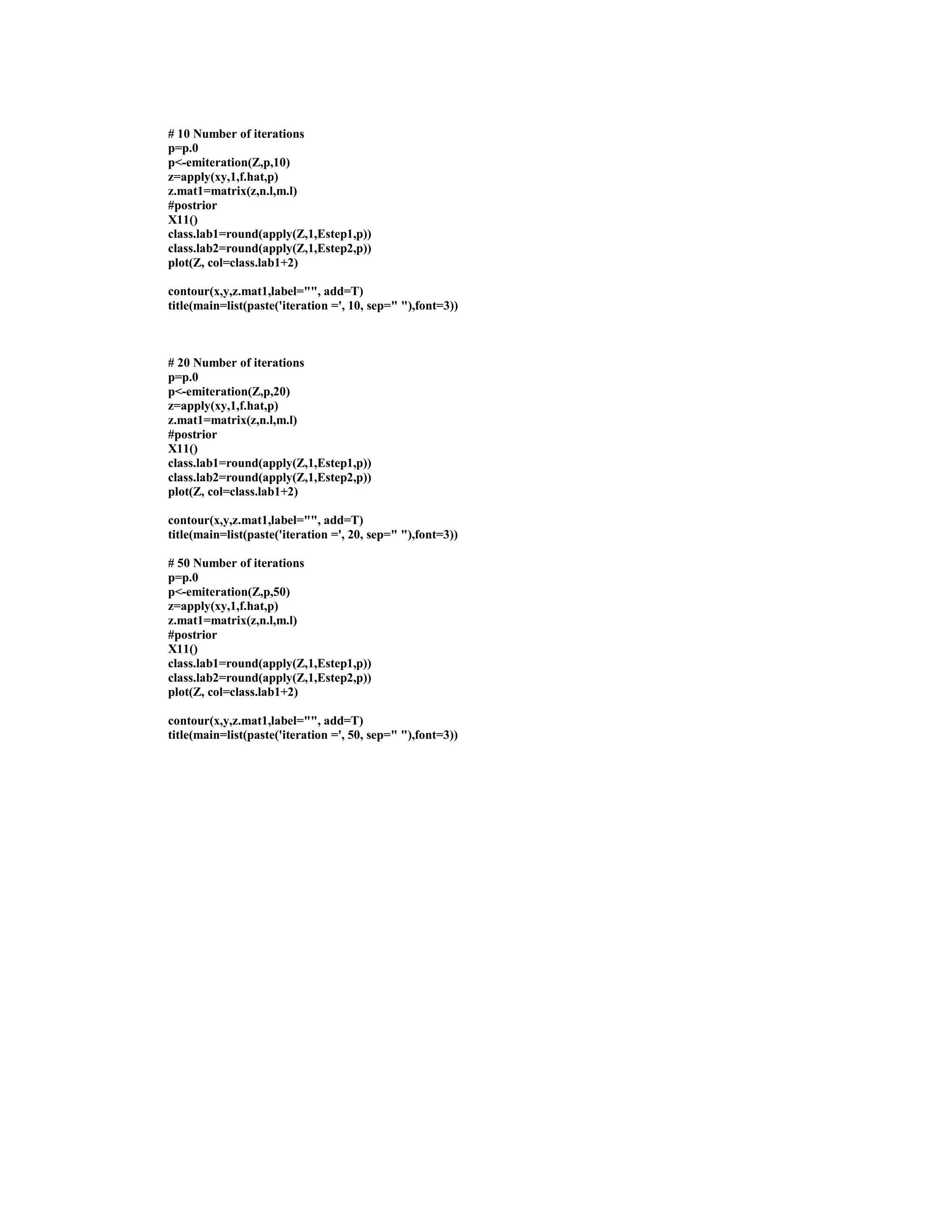
![# 10 Number of Iterations
p=p.0
p<-emiteration(Z,p,10)
z=apply(xy,1,f.hat,p)
z.mat1=matrix(z,n.l,m.l)
#postrior
class.lab1=round(apply(Z,1,Estep,p))
plot(X,Y,xlim=c(40,100),ylim=c(0,6),pch=20,cex=.75,xlab="Waiting time (min)",
ylab='Eruption time (min)',col=class.lab1+2)
contour(x,y,z.mat1,label="", add=T)
title(main=list('iteration = 10',font=3))
# 20 Number of Iterations
p=p.0
p<-emiteration(Z,p,20)
z=apply(xy,1,f.hat,p)
z.mat1=matrix(z,n.l,m.l)
#postrior
class.lab1=round(apply(Z,1,Estep,p))
plot(X,Y,xlim=c(40,100),ylim=c(0,6),pch=20,cex=.75,xlab="Waiting time (min)",
ylab='Eruption time (min)',col=class.lab1+2)
contour(x,y,z.mat1,label="", add=T)
title(main=list('iteration = 20',font=3))
# 50 Number of Iterations
p=p.0
p<-emiteration(Z,p,50)
z=apply(xy,1,f.hat,p)
z.mat1=matrix(z,n.l,m.l)
#postrior
class.lab1=round(apply(Z,1,Estep,p))
plot(X,Y,xlim=c(40,100),ylim=c(0,6),pch=20,cex=.75,xlab="Waiting time (min)",
ylab='Eruption time (min)',col=class.lab1+2)
contour(x,y,z.mat1,label="", add=T)
title(main=list('iteration = 50',font=3))
# Simulated Data for 3 Clusters
#load data
library(mvtnorm)
library(graphics)
library(MASS)
require(ggplot2)
X=rmvnorm(100, mean=c(45,4), sigma=diag(c(2,1)))
Y=rmvnorm(100, mean=c(55,6), sigma=diag(c(2,1)))
U=rmvnorm(100, mean=c(65,7), sigma=diag(c(3,1)))
Z=rbind(X,Y, U)
X11()
km_Z=kmeans(Z,3)$cluster
plot(Z,col=km_Z)
#log-likelihood function
#
ln<-function(p,Y) {
-sum(log(p[1]*dnorm(Y,p[2],sqrt(p[4]))+(1-p[1])*dnorm(Y,p[3],sqrt(p[5]))))
}](https://image.slidesharecdn.com/rcodeforemalgorithm-160506141904/85/R-Code-for-EM-Algorithm-7-320.jpg)
![#
#EM algorithm
#
emstep<-function(Y,p) {
EZ<-p[1]*dnorm(Y,p[2],sqrt(p[4]))/
(p[1]*dnorm(Y,p[2],sqrt(p[4]))
+(1-p[1])*dnorm(Y,p[3],sqrt(p[5])))
p[1]<-mean(EZ)
p[2]<-sum(EZ*Y)/sum(EZ)
p[3]<-sum((1-EZ)*Y)/sum(1-EZ)
p[4]<-sum(EZ*(Y-p[2])^2)/sum(EZ)
p[5]<-sum((1-EZ)*(Y-p[3])^2)/sum(1-EZ)
p
}
emiteration<-function(Y,p,n=2) {
for (i in (1:n)) {
p<-emstep(Y,p)
}
p
}
#density of bivariate normal
#
dbinorm<-function(x,m,s){
1/sqrt(det(2*pi*s))*exp(-0.5*t(x-m)%*%solve(s)%*%(x-m))
}
f.hat<-function(x,p) {
p$p1*dbinorm(x,p$m1,p$s1)+p$p2*dbinorm(x,p$m2,p$s2)+
(1-(p$p1+p$p2))*dbinorm(x, p$m3, p$s3)
}
Estep1<-function(x,p) {
p$p1*dbinorm(x,p$m1,p$s1)/
(p$p1*dbinorm(x,p$m1,p$s1)+p$p2*dbinorm(x,p$m2,p$s2)+
(1-(p$p1+p$p2))*dbinorm(x, p$m3, p$s3))
}
Estep2<-function(x,p){
p$p2*dbinorm(x,p$m2,p$s2)/
(p$p1*dbinorm(x,p$m1,p$s1)+p$p2*dbinorm(x,p$m2,p$s2)+
(1-(p$p1+p$p2))*dbinorm(x, p$m3, p$s3))
}
Estep3<-function(x,p){
p$p3*dbinorm(x,p$m3,p$s3)/
(p$p1*dbinorm(x,p$m1,p$s1)+p$p2*dbinorm(x,p$m2,p$s2)+
p$p3*dbinorm(x, p$m3, p$s3))
}
emstep<-function(Y,p){
EZ1<-apply(Y,1,Estep1,p)
EZ2<-apply(Y,1,Estep2,p)
p$p1<-mean(EZ1)
p$p2<-mean(EZ2)
p$m1<-(t(Y)%*%diag(EZ1)%*%rep(1,nrow(Y)))/sum(EZ1)
p$m2<-(t(Y)%*%diag(EZ2)%*%rep(1,nrow(Y)))/sum(EZ2)
p$m3<-(t(Y)%*%diag(1-(EZ1+EZ2))%*%rep(1,nrow(Y)))/sum(1-(EZ1+EZ2))
MY<-matrix(p$m1,nrow(Y),2,byrow=T)
p$s1<-(t(Y-MY)%*%diag(EZ1)%*%(Y-MY))/sum(EZ1)
MY<-matrix(p$m2,nrow(Y),2,byrow=T)
p$s2<-(t(Y-MY)%*%diag(EZ2)%*%(Y-MY))/sum(EZ2)
MY<-matrix(p$m3,nrow(Y),2,byrow=T)
p$s3<-(t(Y-MY)%*%diag(1-(EZ1+EZ2))%*%(Y-MY))/sum(1-(EZ1+EZ2))
p
}
emiteration<-function(Y,p,n=10) {
for (i in (1:n)) {
p<-emstep(Y,p)
}](https://image.slidesharecdn.com/rcodeforemalgorithm-160506141904/85/R-Code-for-EM-Algorithm-8-320.jpg)
![p
}
#starting values
#
p=p.0<-list(p1=1/3,p2=1/3,p3=1/3,m1=c(45,2),m2=c(60,4),m3=c(70,8),
s1=matrix(c(1,0,0,1),2,2),s2=matrix(c(1,0,0,1),2,2),
s3=matrix(c(1,0,0,1),2,2))
#--------------------------------------
lh=NULL
P=matrix(0,20,length(p))
for(i in 1:20){
p<-emiteration(Z,p,i)
lh[i]=sum(log(apply(Z,1,f.hat,p)))
}
X11()
plot(lh,type='o',xlab='iterations',ylab='likelihood')
#---------------------------------------
#---Graph the mixture:
n.l=m.l=30
x=seq(30,70,length= n.l)
y=seq(0,10,length = m.l)
xy=as.matrix(expand.grid(x,y))
# 1 Number of iterations
p=p.0
p<-emiteration(Z,p,1)
z=apply(xy,1,f.hat,p)
z.mat1=matrix(z,n.l,m.l)
#postrior
X11()
class.lab1=round(apply(Z,1,Estep1,p))
class.lab2=round(apply(Z,1,Estep2,p))
plot(Z, col=class.lab1+2)
contour(x,y,z.mat1,label="", add=T)
title(main=list(paste('iteration =', 1, sep=" "),font=3))
# 2 Number of iterations
p=p.0
p<-emiteration(Z,p,2)
z=apply(xy,1,f.hat,p)
z.mat1=matrix(z,n.l,m.l)
#postrior
X11()
class.lab1=round(apply(Z,1,Estep1,p))
class.lab2=round(apply(Z,1,Estep2,p))
plot(Z, col=class.lab1+2)
contour(x,y,z.mat1,label="", add=T)
title(main=list(paste('iteration =', 2, sep=" "),font=3))
# 5 Number of iterations
p=p.0
p<-emiteration(Z,p,5)
z=apply(xy,1,f.hat,p)
z.mat1=matrix(z,n.l,m.l)
#postrior
X11()
class.lab1=round(apply(Z,1,Estep1,p))
class.lab2=round(apply(Z,1,Estep2,p))
plot(Z, col=class.lab1+2)
contour(x,y,z.mat1,label="", add=T)
title(main=list(paste('iteration =', 5, sep=" "),font=3))](https://image.slidesharecdn.com/rcodeforemalgorithm-160506141904/85/R-Code-for-EM-Algorithm-9-320.jpg)

![#FaithFUL Dataset 1D
#
#load data
#
data(faithful)
Y<-faithful$waiting
#
#plot histogram of waiting times
#
postscript("geyser.eps",width=5,height=3,onefile=F)
par(mar=c(2,2,1,1),mgp=c(1,0.5,0),cex=0.7,lwd=0.5,las=1)
hist(Y,breaks=seq(40,100,3),xlab="Waiting time between eruptions (min)",
xlim=c(40,100),main="",axes=F)
axis(1,seq(40,100,6),pos=0)
axis(2,seq(0,35,5),pos=40,las=1)
dev.off()
#
#log-likelihood function
#
ln<-function(p,Y) {
-sum(log(p[1]*dnorm(Y,p[2],sqrt(p[4]))+(1-p[1])*dnorm(Y,p[3],sqrt(p[5]))))
}
#
#EM algorithm
#
emstep<-function(Y,p) {
EZ<-p[1]*dnorm(Y,p[2],sqrt(p[4]))/
(p[1]*dnorm(Y,p[2],sqrt(p[4]))
+(1-p[1])*dnorm(Y,p[3],sqrt(p[5])))
p[1]<-mean(EZ)
p[2]<-sum(EZ*Y)/sum(EZ)
p[3]<-sum((1-EZ)*Y)/sum(1-EZ)
p[4]<-sum(EZ*(Y-p[2])^2)/sum(EZ)
p[5]<-sum((1-EZ)*(Y-p[3])^2)/sum(1-EZ)
p
}
emiteration<-function(Y,p,n=10) {
for (i in (1:n)) {
p<-emstep(Y,p)
}
p
}
#
#starting values
#
p<-c(0.5,40,90,16,16)
#
#2 iterations of EM algorithm
#
p<-emiteration(Y,p,2)
p
#check for convergence
p<-emstep(Y,p)
p
#
#plot histogram with fitted distribution
#
hist(Y,breaks=seq(40,100,3),xlab="Waiting time between eruptions (min)",
xlim=c(40,100),
main="",axes=F)
axis(1,seq(40,100,6),pos=0)](https://image.slidesharecdn.com/rcodeforemalgorithm-160506141904/75/R-Code-for-EM-Algorithm-3-2048.jpg)
![axis(2,seq(0,35,5),pos=40,las=1)
x<-seq(40,100,0.1)
y<-p[1]*dnorm(x,p[2],sqrt(p[4]))+(1-p[1])*dnorm(x,p[3],sqrt(p[5]))
lines(x,y*3*length(Y))
#5 iterations of EM algorithm
#log-likelihood function
#
ln<-function(p,Y) {
-sum(log(p[1]*dnorm(Y,p[2],sqrt(p[4]))+(1-p[1])*dnorm(Y,p[3],sqrt(p[5]))))
}
#
#EM algorithm
#
emstep<-function(Y,p) {
EZ<-p[1]*dnorm(Y,p[2],sqrt(p[4]))/
(p[1]*dnorm(Y,p[2],sqrt(p[4]))
+(1-p[1])*dnorm(Y,p[3],sqrt(p[5])))
p[1]<-mean(EZ)
p[2]<-sum(EZ*Y)/sum(EZ)
p[3]<-sum((1-EZ)*Y)/sum(1-EZ)
p[4]<-sum(EZ*(Y-p[2])^2)/sum(EZ)
p[5]<-sum((1-EZ)*(Y-p[3])^2)/sum(1-EZ)
p
}
emiteration<-function(Y,p,n=10) {
for (i in (1:n)) {
p<-emstep(Y,p)
}
p
}
#
#starting values
#
p<-c(0.5,40,90,16,16)
#
#5 iterations of EM algorithm
#
p<-emiteration(Y,p,5)
p
#check for convergence
p<-emstep(Y,p)
p
#
#plot histogram with fitted distribution
#
hist(Y,breaks=seq(40,100,3),xlab="Waiting time between eruptions (min)",
xlim=c(40,100),
main="",axes=F)
axis(1,seq(40,100,6),pos=0)
axis(2,seq(0,35,5),pos=40,las=1)
x<-seq(40,100,0.1)
y<-p[1]*dnorm(x,p[2],sqrt(p[4]))+(1-p[1])*dnorm(x,p[3],sqrt(p[5]))
lines(x,y*3*length(Y))
#10 iterations of EM algorithm
#log-likelihood function
#
ln<-function(p,Y) {
-sum(log(p[1]*dnorm(Y,p[2],sqrt(p[4]))+(1-p[1])*dnorm(Y,p[3],sqrt(p[5]))))
}
#
#EM algorithm
#
emstep<-function(Y,p) {
EZ<-p[1]*dnorm(Y,p[2],sqrt(p[4]))/
(p[1]*dnorm(Y,p[2],sqrt(p[4]))
+(1-p[1])*dnorm(Y,p[3],sqrt(p[5])))](https://image.slidesharecdn.com/rcodeforemalgorithm-160506141904/75/R-Code-for-EM-Algorithm-4-2048.jpg)
![p[1]<-mean(EZ)
p[2]<-sum(EZ*Y)/sum(EZ)
p[3]<-sum((1-EZ)*Y)/sum(1-EZ)
p[4]<-sum(EZ*(Y-p[2])^2)/sum(EZ)
p[5]<-sum((1-EZ)*(Y-p[3])^2)/sum(1-EZ)
p
}
emiteration<-function(Y,p,n=10) {
for (i in (1:n)) {
p<-emstep(Y,p)
}
p
}
#
#starting values
#
p<-c(0.5,40,90,16,16)
#
#10 iterations of EM algorithm
#
p<-emiteration(Y,p,10)
p
#check for convergence
p<-emstep(Y,p)
p
#
#plot histogram with fitted distribution
#
hist(Y,breaks=seq(40,100,3),xlab="Waiting time between eruptions (min)",
xlim=c(40,100),
main="",axes=F)
axis(1,seq(40,100,6),pos=0)
axis(2,seq(0,35,5),pos=40,las=1)
x<-seq(40,100,0.1)
y<-p[1]*dnorm(x,p[2],sqrt(p[4]))+(1-p[1])*dnorm(x,p[3],sqrt(p[5]))
lines(x,y*3*length(Y))
#Faithful Dataset 2D
#load data
#
#
#Bivariate mixture model
#
data(faithful)
Y<-faithful$waiting
X<-faithful$eruptions
plot(Y,X,xlab="Waiting time between eruptions (min)",
ylab="Eruption times (min)",
xlim=c(40,100),ylim=c(0,6),
main="",axes=F,cex=0.7)
axis(1,seq(40,100,6),pos=0)
axis(2,seq(0,6,1),pos=40,las=1)
#
#density of bivariate normal
#
dbinorm<-function(x,m,s){
1/sqrt(det(2*pi*s))*exp(-0.5*t(x-m)%*%solve(s)%*%(x-m))
}
f.hat<-function(x,p) {
p$p*dbinorm(x,p$m1,p$s1)+(1-p$p)*dbinorm(x,p$m2,p$s2)
}
Estep<-function(x,p) {
p$p*dbinorm(x,p$m1,p$s1)/](https://image.slidesharecdn.com/rcodeforemalgorithm-160506141904/75/R-Code-for-EM-Algorithm-5-2048.jpg)
![(p$p*dbinorm(x,p$m1,p$s1)
+(1-p$p)*dbinorm(x,p$m2,p$s2))
}
emstep<-function(Y,p) {
EZ<-apply(Y,1,Estep,p)
p$p<-mean(EZ)
p$m1<-(t(Y)%*%diag(EZ)%*%rep(1,nrow(Y)))/sum(EZ)
p$m2<-(t(Y)%*%diag(1-EZ)%*%rep(1,nrow(Y)))/sum(1-EZ)
MY<-matrix(p$m1,nrow(Y),2,byrow=T)
p$s1<-(t(Y-MY)%*%diag(EZ)%*%(Y-MY))/sum(EZ)
MY<-matrix(p$m2,nrow(Y),2,byrow=T)
p$s2<-(t(Y-MY)%*%diag(1-EZ)%*%(Y-MY))/sum(1-EZ)
p
}
#----------------------------------
X<-faithful$waiting
Y<-faithful$eruptions
Z<-cbind(X,Y)
#starting values
#
p=p.0<-list(p=0.5,m1=c(20,6),m2=c(70,6),
s1=matrix(c(10,0,0,1),2,2),s2=matrix(c(10,0,0,1),2,2))
#--------------------------------------
lh=NULL
P=matrix(0,20,length(p))
for(i in 1:20){
p<-emiteration(Z,p,i)
lh[i]=sum(log(apply(Z,1,f.hat,p)))
}
plot(lh,type='o',xlab='iterations',ylab='likelihood')
#---------------------------------------
require(ggplot2)
#---Graph the mixture:
n.l=m.l=30
x=seq(40,100,length= n.l)
y=seq(0,6,length = m.l)
xy=as.matrix(expand.grid(x,y))
# 2 Number of Iterations
p=p.0
p<-emiteration(Z,p,2)
z=apply(xy,1,f.hat,p)
z.mat1=matrix(z,n.l,m.l)
#postrior
class.lab1=round(apply(Z,1,Estep,p))
plot(X,Y,xlim=c(40,100),ylim=c(0,6),pch=20,cex=.75,xlab="Waiting time (min)",
ylab='Eruption time (min)',col=class.lab1+2)
contour(x,y,z.mat1,label="", add=T)
title(main=list('iteration = 2',font=3))
# 5 Number of Iterations
p=p.0
p<-emiteration(Z,p,5)
z=apply(xy,1,f.hat,p)
z.mat1=matrix(z,n.l,m.l)
#postrior
class.lab1=round(apply(Z,1,Estep,p))
plot(X,Y,xlim=c(40,100),ylim=c(0,6),pch=20,cex=.75,xlab="Waiting time (min)",
ylab='Eruption time (min)',col=class.lab1+2)
contour(x,y,z.mat1,label="", add=T)
title(main=list('iteration = 5',font=3))](https://image.slidesharecdn.com/rcodeforemalgorithm-160506141904/75/R-Code-for-EM-Algorithm-6-2048.jpg)
![# 10 Number of Iterations
p=p.0
p<-emiteration(Z,p,10)
z=apply(xy,1,f.hat,p)
z.mat1=matrix(z,n.l,m.l)
#postrior
class.lab1=round(apply(Z,1,Estep,p))
plot(X,Y,xlim=c(40,100),ylim=c(0,6),pch=20,cex=.75,xlab="Waiting time (min)",
ylab='Eruption time (min)',col=class.lab1+2)
contour(x,y,z.mat1,label="", add=T)
title(main=list('iteration = 10',font=3))
# 20 Number of Iterations
p=p.0
p<-emiteration(Z,p,20)
z=apply(xy,1,f.hat,p)
z.mat1=matrix(z,n.l,m.l)
#postrior
class.lab1=round(apply(Z,1,Estep,p))
plot(X,Y,xlim=c(40,100),ylim=c(0,6),pch=20,cex=.75,xlab="Waiting time (min)",
ylab='Eruption time (min)',col=class.lab1+2)
contour(x,y,z.mat1,label="", add=T)
title(main=list('iteration = 20',font=3))
# 50 Number of Iterations
p=p.0
p<-emiteration(Z,p,50)
z=apply(xy,1,f.hat,p)
z.mat1=matrix(z,n.l,m.l)
#postrior
class.lab1=round(apply(Z,1,Estep,p))
plot(X,Y,xlim=c(40,100),ylim=c(0,6),pch=20,cex=.75,xlab="Waiting time (min)",
ylab='Eruption time (min)',col=class.lab1+2)
contour(x,y,z.mat1,label="", add=T)
title(main=list('iteration = 50',font=3))
# Simulated Data for 3 Clusters
#load data
library(mvtnorm)
library(graphics)
library(MASS)
require(ggplot2)
X=rmvnorm(100, mean=c(45,4), sigma=diag(c(2,1)))
Y=rmvnorm(100, mean=c(55,6), sigma=diag(c(2,1)))
U=rmvnorm(100, mean=c(65,7), sigma=diag(c(3,1)))
Z=rbind(X,Y, U)
X11()
km_Z=kmeans(Z,3)$cluster
plot(Z,col=km_Z)
#log-likelihood function
#
ln<-function(p,Y) {
-sum(log(p[1]*dnorm(Y,p[2],sqrt(p[4]))+(1-p[1])*dnorm(Y,p[3],sqrt(p[5]))))
}](https://image.slidesharecdn.com/rcodeforemalgorithm-160506141904/75/R-Code-for-EM-Algorithm-7-2048.jpg)
![#
#EM algorithm
#
emstep<-function(Y,p) {
EZ<-p[1]*dnorm(Y,p[2],sqrt(p[4]))/
(p[1]*dnorm(Y,p[2],sqrt(p[4]))
+(1-p[1])*dnorm(Y,p[3],sqrt(p[5])))
p[1]<-mean(EZ)
p[2]<-sum(EZ*Y)/sum(EZ)
p[3]<-sum((1-EZ)*Y)/sum(1-EZ)
p[4]<-sum(EZ*(Y-p[2])^2)/sum(EZ)
p[5]<-sum((1-EZ)*(Y-p[3])^2)/sum(1-EZ)
p
}
emiteration<-function(Y,p,n=2) {
for (i in (1:n)) {
p<-emstep(Y,p)
}
p
}
#density of bivariate normal
#
dbinorm<-function(x,m,s){
1/sqrt(det(2*pi*s))*exp(-0.5*t(x-m)%*%solve(s)%*%(x-m))
}
f.hat<-function(x,p) {
p$p1*dbinorm(x,p$m1,p$s1)+p$p2*dbinorm(x,p$m2,p$s2)+
(1-(p$p1+p$p2))*dbinorm(x, p$m3, p$s3)
}
Estep1<-function(x,p) {
p$p1*dbinorm(x,p$m1,p$s1)/
(p$p1*dbinorm(x,p$m1,p$s1)+p$p2*dbinorm(x,p$m2,p$s2)+
(1-(p$p1+p$p2))*dbinorm(x, p$m3, p$s3))
}
Estep2<-function(x,p){
p$p2*dbinorm(x,p$m2,p$s2)/
(p$p1*dbinorm(x,p$m1,p$s1)+p$p2*dbinorm(x,p$m2,p$s2)+
(1-(p$p1+p$p2))*dbinorm(x, p$m3, p$s3))
}
Estep3<-function(x,p){
p$p3*dbinorm(x,p$m3,p$s3)/
(p$p1*dbinorm(x,p$m1,p$s1)+p$p2*dbinorm(x,p$m2,p$s2)+
p$p3*dbinorm(x, p$m3, p$s3))
}
emstep<-function(Y,p){
EZ1<-apply(Y,1,Estep1,p)
EZ2<-apply(Y,1,Estep2,p)
p$p1<-mean(EZ1)
p$p2<-mean(EZ2)
p$m1<-(t(Y)%*%diag(EZ1)%*%rep(1,nrow(Y)))/sum(EZ1)
p$m2<-(t(Y)%*%diag(EZ2)%*%rep(1,nrow(Y)))/sum(EZ2)
p$m3<-(t(Y)%*%diag(1-(EZ1+EZ2))%*%rep(1,nrow(Y)))/sum(1-(EZ1+EZ2))
MY<-matrix(p$m1,nrow(Y),2,byrow=T)
p$s1<-(t(Y-MY)%*%diag(EZ1)%*%(Y-MY))/sum(EZ1)
MY<-matrix(p$m2,nrow(Y),2,byrow=T)
p$s2<-(t(Y-MY)%*%diag(EZ2)%*%(Y-MY))/sum(EZ2)
MY<-matrix(p$m3,nrow(Y),2,byrow=T)
p$s3<-(t(Y-MY)%*%diag(1-(EZ1+EZ2))%*%(Y-MY))/sum(1-(EZ1+EZ2))
p
}
emiteration<-function(Y,p,n=10) {
for (i in (1:n)) {
p<-emstep(Y,p)
}](https://image.slidesharecdn.com/rcodeforemalgorithm-160506141904/75/R-Code-for-EM-Algorithm-8-2048.jpg)
![p
}
#starting values
#
p=p.0<-list(p1=1/3,p2=1/3,p3=1/3,m1=c(45,2),m2=c(60,4),m3=c(70,8),
s1=matrix(c(1,0,0,1),2,2),s2=matrix(c(1,0,0,1),2,2),
s3=matrix(c(1,0,0,1),2,2))
#--------------------------------------
lh=NULL
P=matrix(0,20,length(p))
for(i in 1:20){
p<-emiteration(Z,p,i)
lh[i]=sum(log(apply(Z,1,f.hat,p)))
}
X11()
plot(lh,type='o',xlab='iterations',ylab='likelihood')
#---------------------------------------
#---Graph the mixture:
n.l=m.l=30
x=seq(30,70,length= n.l)
y=seq(0,10,length = m.l)
xy=as.matrix(expand.grid(x,y))
# 1 Number of iterations
p=p.0
p<-emiteration(Z,p,1)
z=apply(xy,1,f.hat,p)
z.mat1=matrix(z,n.l,m.l)
#postrior
X11()
class.lab1=round(apply(Z,1,Estep1,p))
class.lab2=round(apply(Z,1,Estep2,p))
plot(Z, col=class.lab1+2)
contour(x,y,z.mat1,label="", add=T)
title(main=list(paste('iteration =', 1, sep=" "),font=3))
# 2 Number of iterations
p=p.0
p<-emiteration(Z,p,2)
z=apply(xy,1,f.hat,p)
z.mat1=matrix(z,n.l,m.l)
#postrior
X11()
class.lab1=round(apply(Z,1,Estep1,p))
class.lab2=round(apply(Z,1,Estep2,p))
plot(Z, col=class.lab1+2)
contour(x,y,z.mat1,label="", add=T)
title(main=list(paste('iteration =', 2, sep=" "),font=3))
# 5 Number of iterations
p=p.0
p<-emiteration(Z,p,5)
z=apply(xy,1,f.hat,p)
z.mat1=matrix(z,n.l,m.l)
#postrior
X11()
class.lab1=round(apply(Z,1,Estep1,p))
class.lab2=round(apply(Z,1,Estep2,p))
plot(Z, col=class.lab1+2)
contour(x,y,z.mat1,label="", add=T)
title(main=list(paste('iteration =', 5, sep=" "),font=3))](https://image.slidesharecdn.com/rcodeforemalgorithm-160506141904/75/R-Code-for-EM-Algorithm-9-2048.jpg)

This R code document contains code for implementing the Expectation-Maximization (EM) algorithm for Gaussian mixture models with 1, 2, and 3 clusters of data. The code includes functions for the EM steps, starting values, and plotting the results. It applies the EM algorithm to real datasets with 1 and 2 dimensions and to a simulated 3 cluster dataset.
Presentation introduces R code for the Expectation-Maximization (EM) algorithm for Gaussian mixtures, covering 1D, 2D data, and multiple clusters.
Explains the iterative EM algorithm process involving E-steps and M-steps to find maximum likelihood estimates, along with convergence detection using log-likelihood.
Presents an application of EM algorithm on the 1D Faithful dataset, including data loading, histogram plotting, log-likelihood function, and two EM iterations.
Further iterations of the EM algorithm on the 1D Faithful dataset are conducted; includes plotting of distributions using histogram and fitted curve for convergence checks.
Describes the application of the EM algorithm on the 2D structure of the Faithful dataset, involving data preparation, plotting eruption times and waiting times.
Develops further on 2D Gaussian mixtures using EM algorithm with multiple iterations (2, 5, 10, 20), demonstrating the fitting of distributions through contour plots.
Introduces simulated data for three clusters and extends the EM algorithm, detailing likelihood calculation and visualizing results for multiple iterations.


![Agentic Systems and Compliance - A brief intro [1.2]](https://cdn.slidesharecdn.com/ss_thumbnails/agenticsystemsandcompliace-1-251018025303-958a42ec-thumbnail.jpg?width=600ounds&width=560&fit=bounds)


![Matrix and determinant URT [Autosaved].pptx](https://cdn.slidesharecdn.com/ss_thumbnails/matrixanddeterminanturtautosaved-251018190340-9e6a6deb-thumbnail.jpg?width=600ounds&width=560&fit=bounds)


