Downloaded 92 times


The document discusses correlation and regression, emphasizing their roles in statistical analysis to identify relationships between quantitative variables. It illustrates concepts such as positive and negative correlations, correlation coefficients, and the calculation of regression equations. The document provides examples and explanations of both simple and Spearman rank correlation methodologies, as well as regression analysis for predictive modeling.
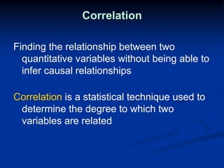
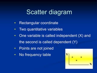
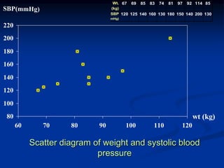
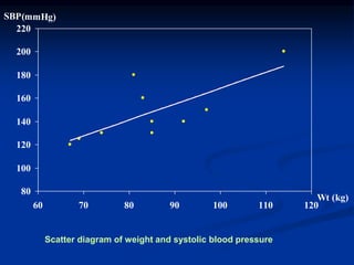
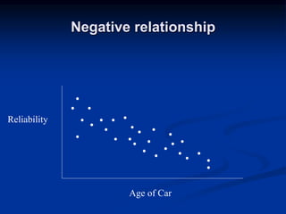
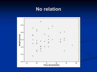
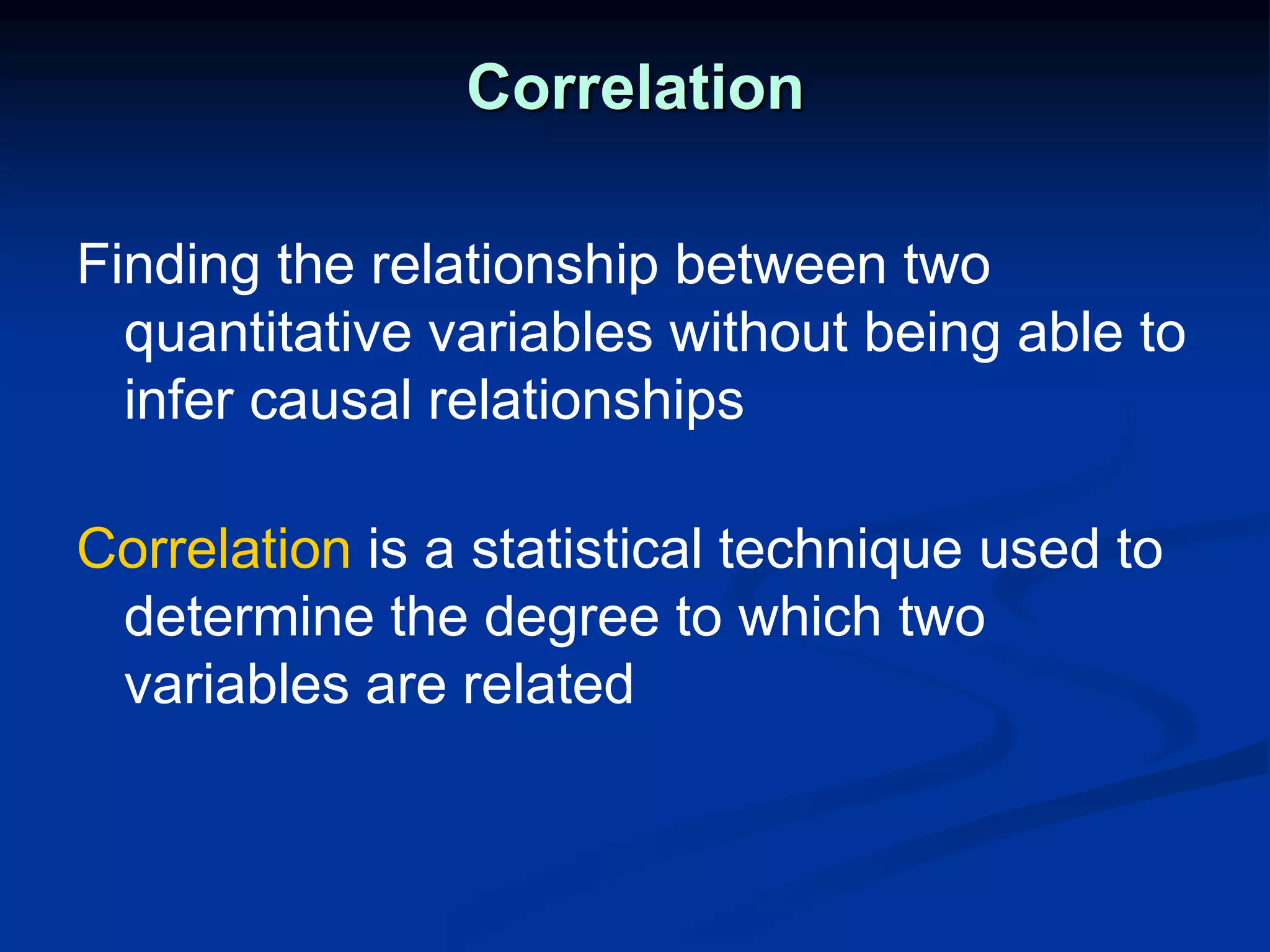
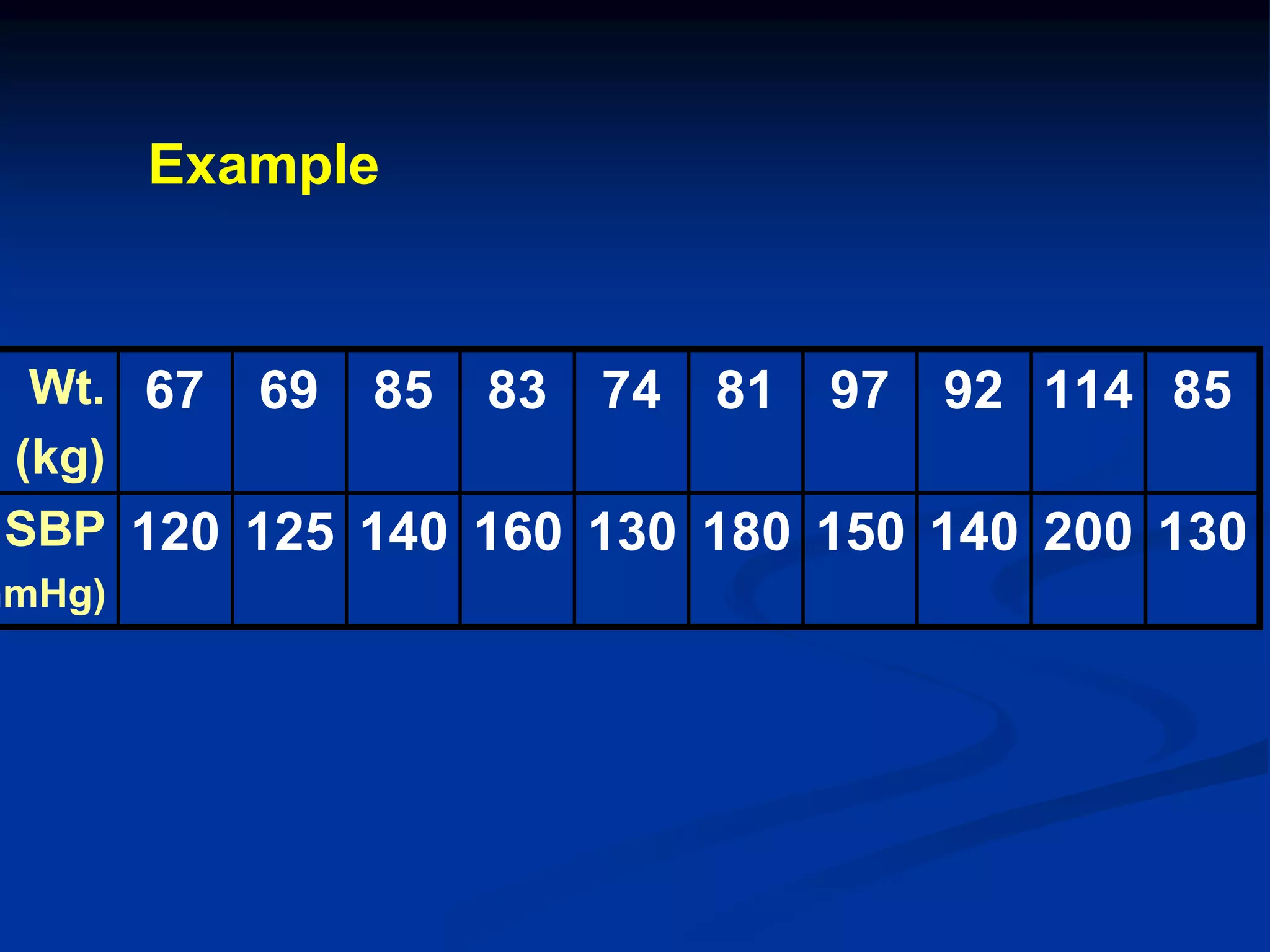
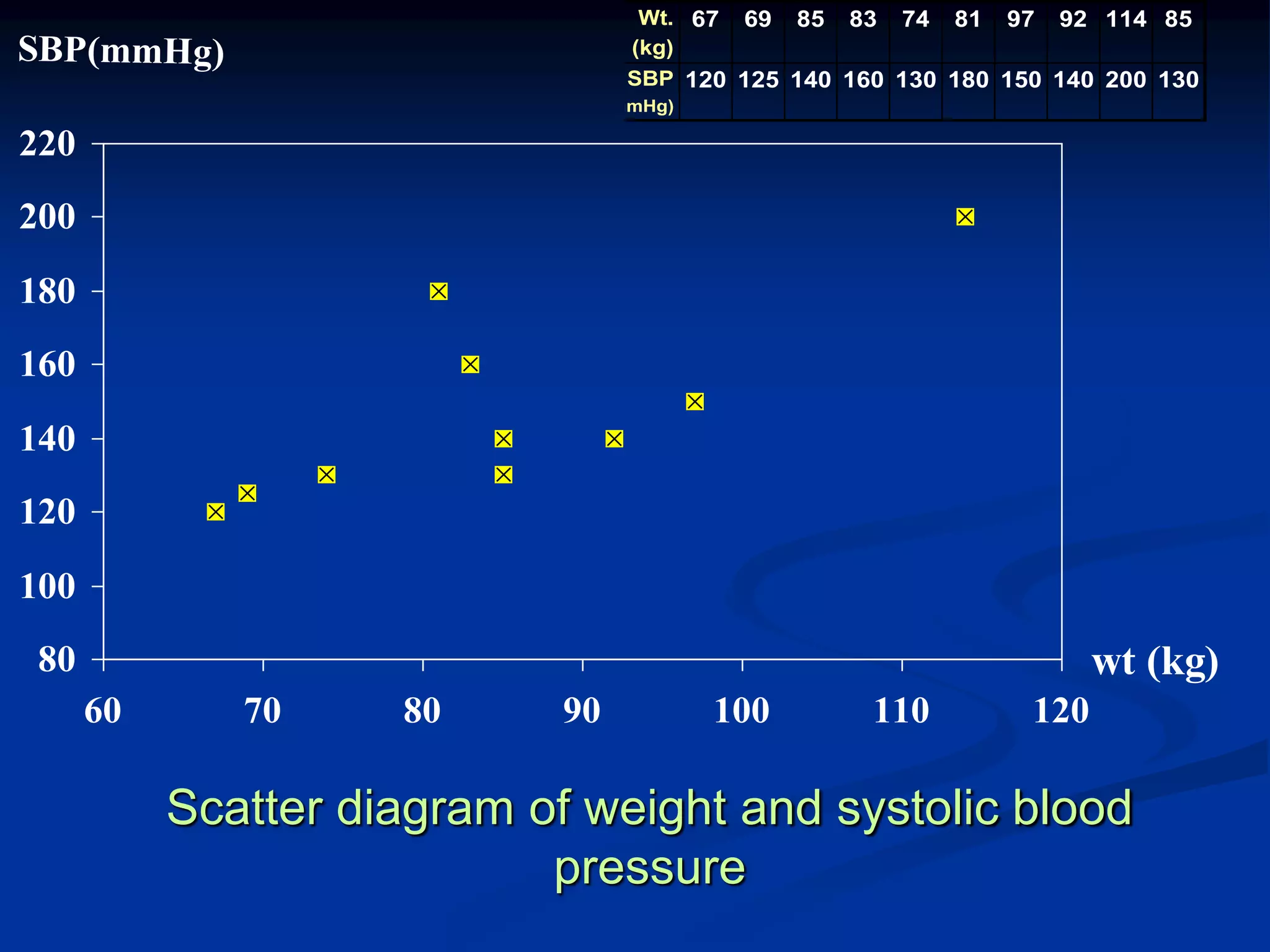
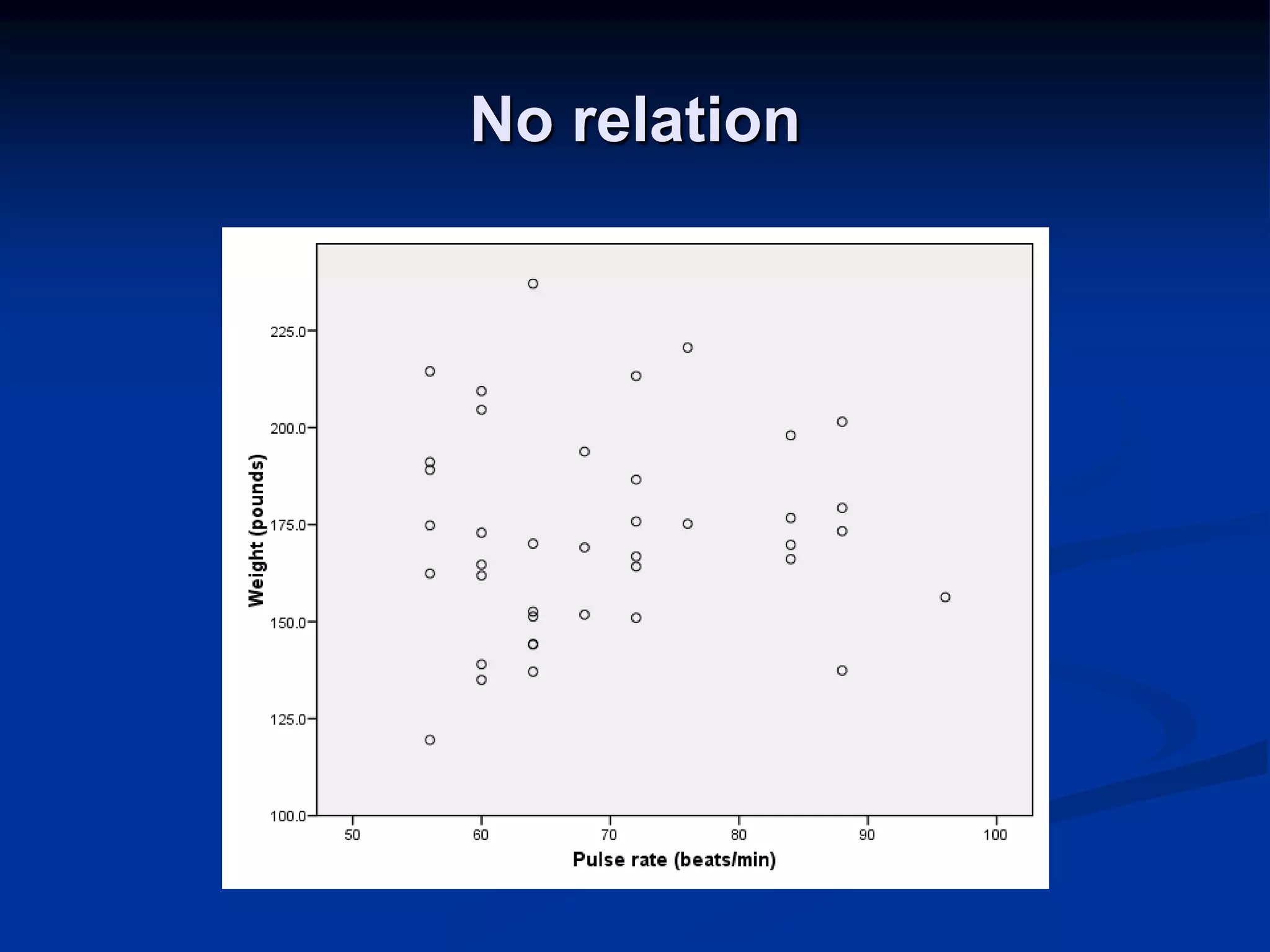
Focus on defining correlation and scatter diagrams to analyze the relationship between quantitative variables.
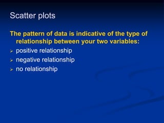
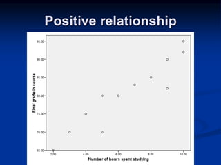
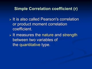
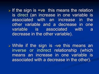
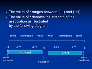
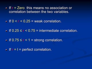
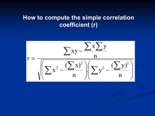
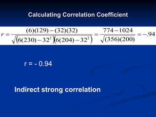
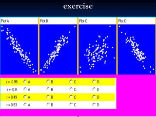
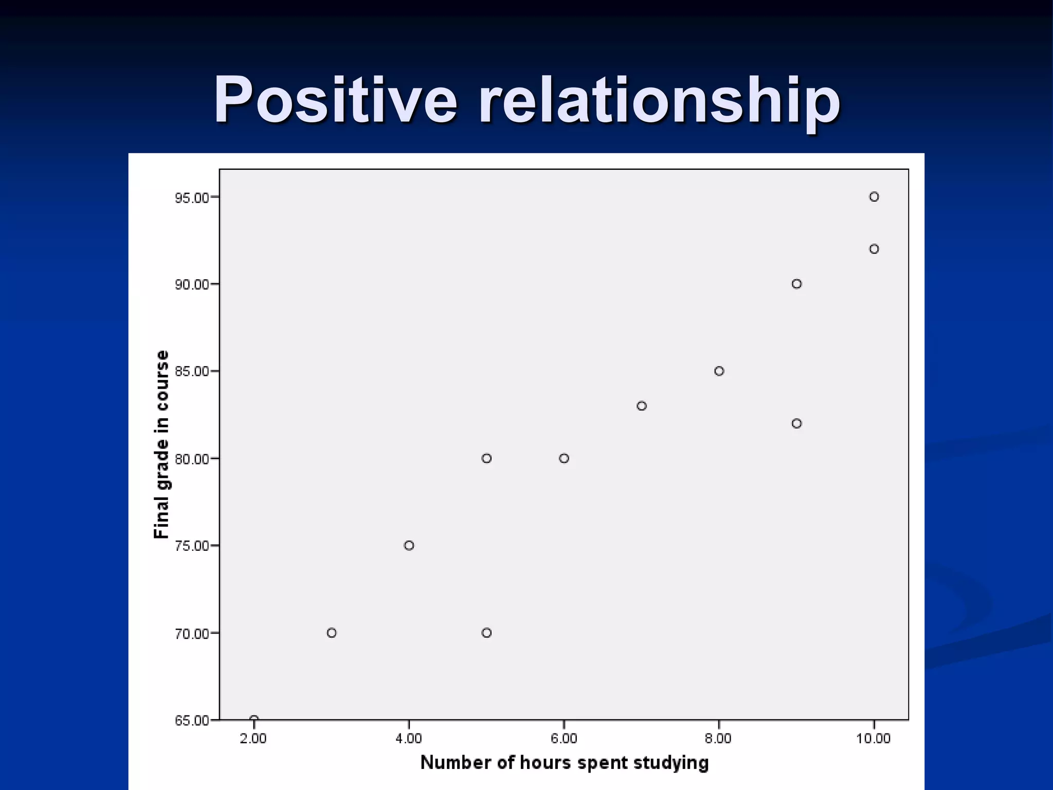
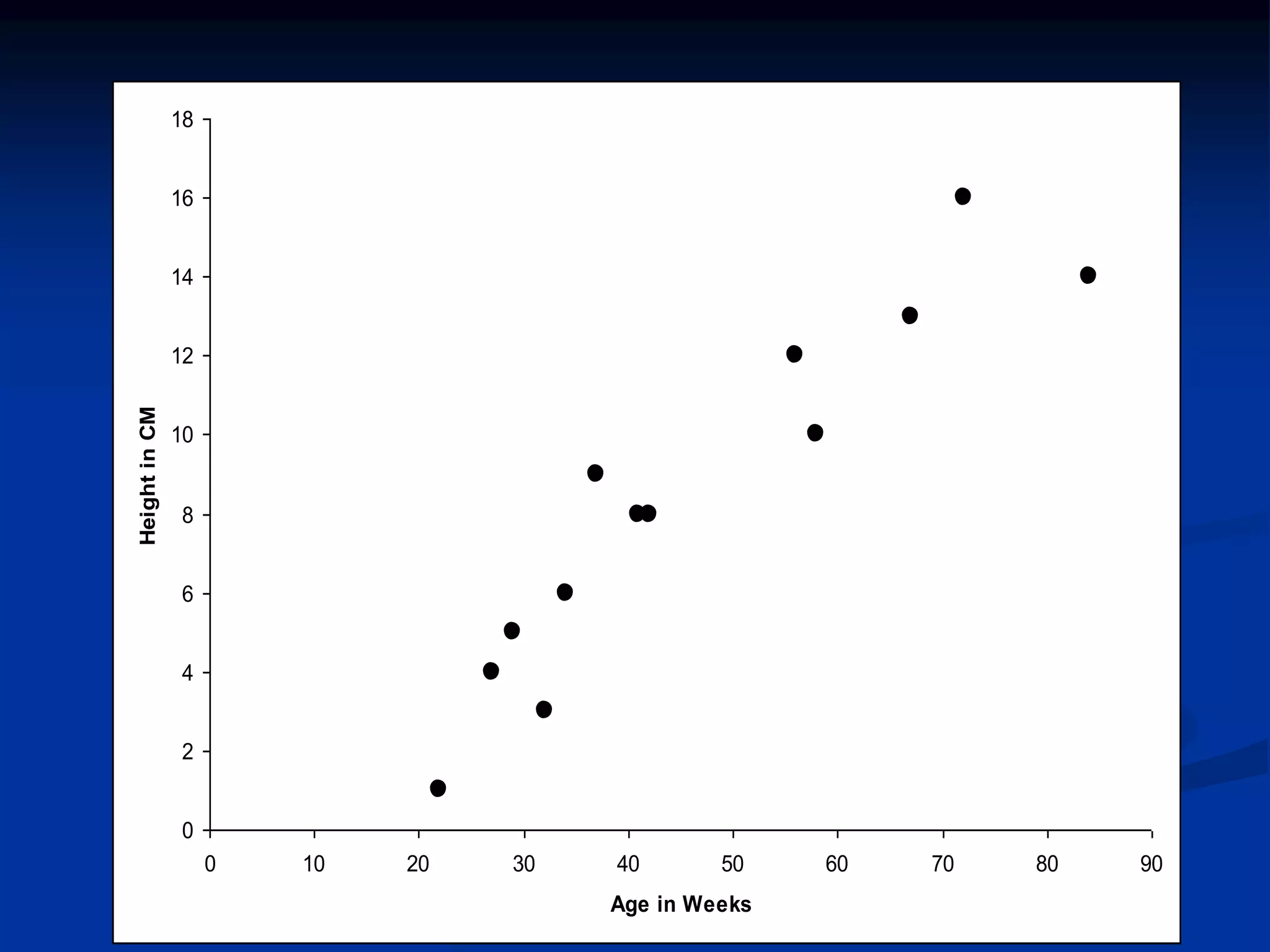
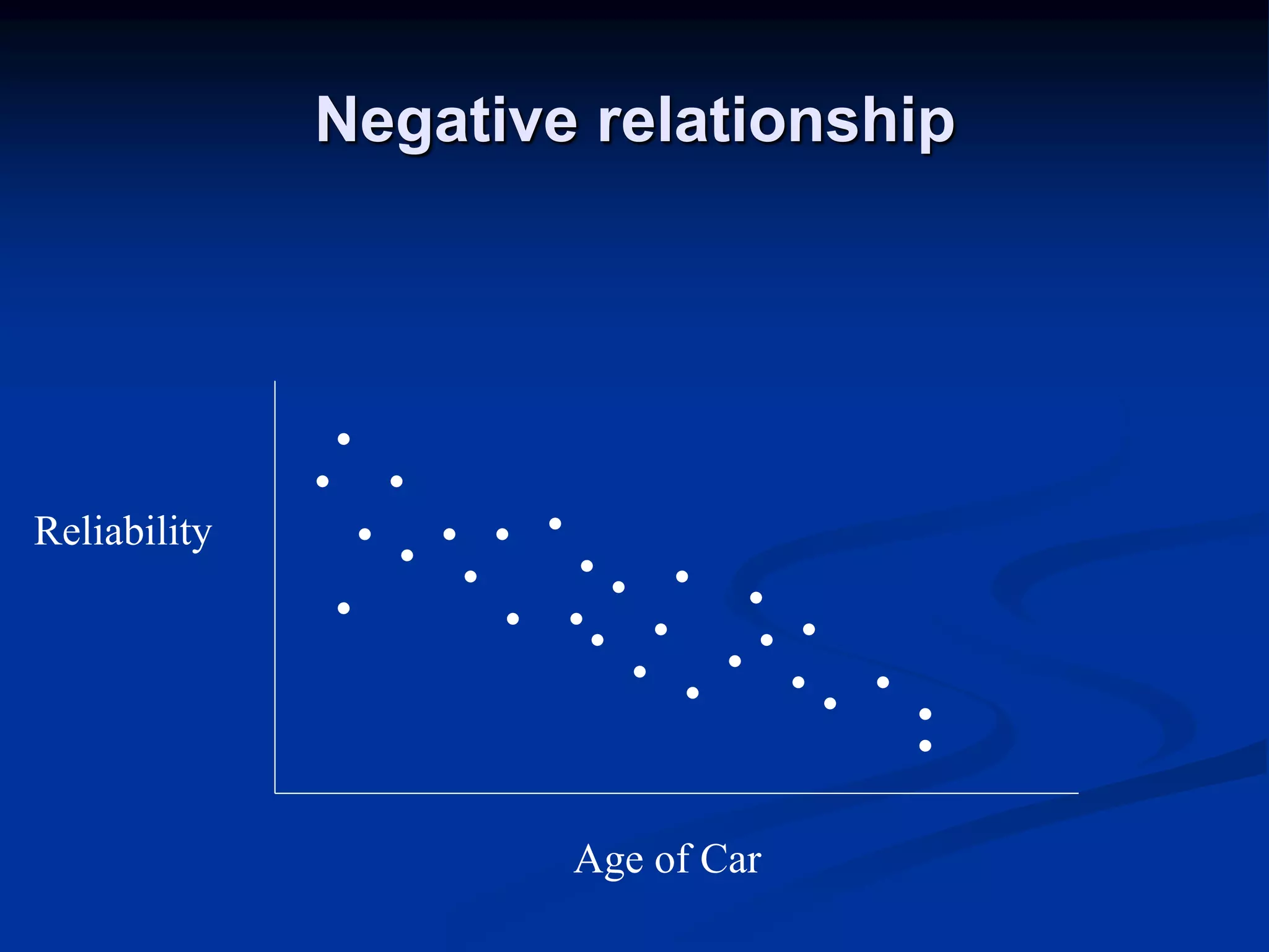
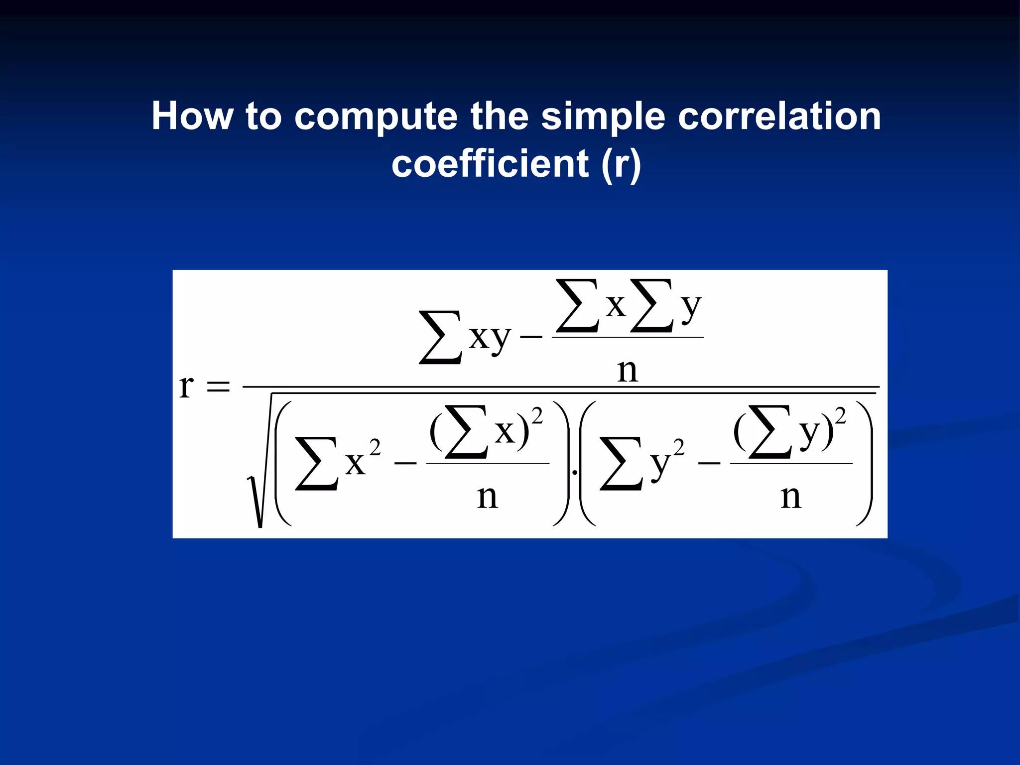
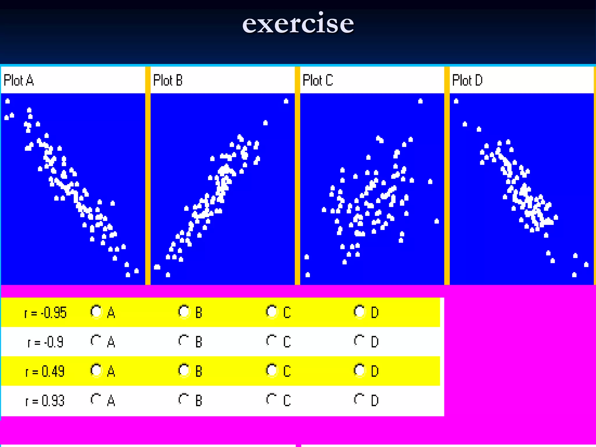
Discusses correlation types (positive, negative, no relation) and computes correlation coefficients to quantify relationships.
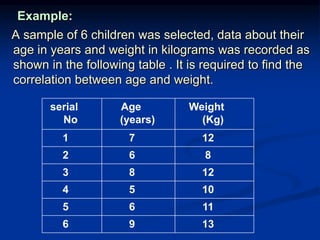
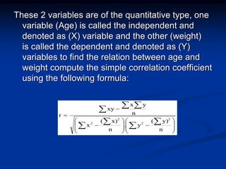
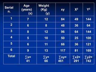
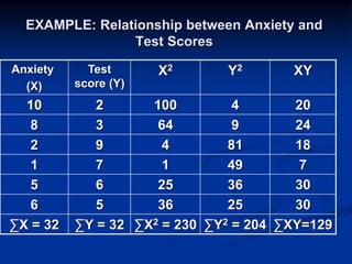
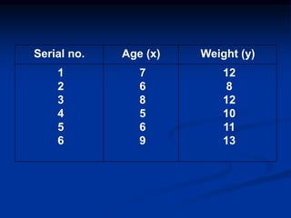
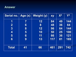
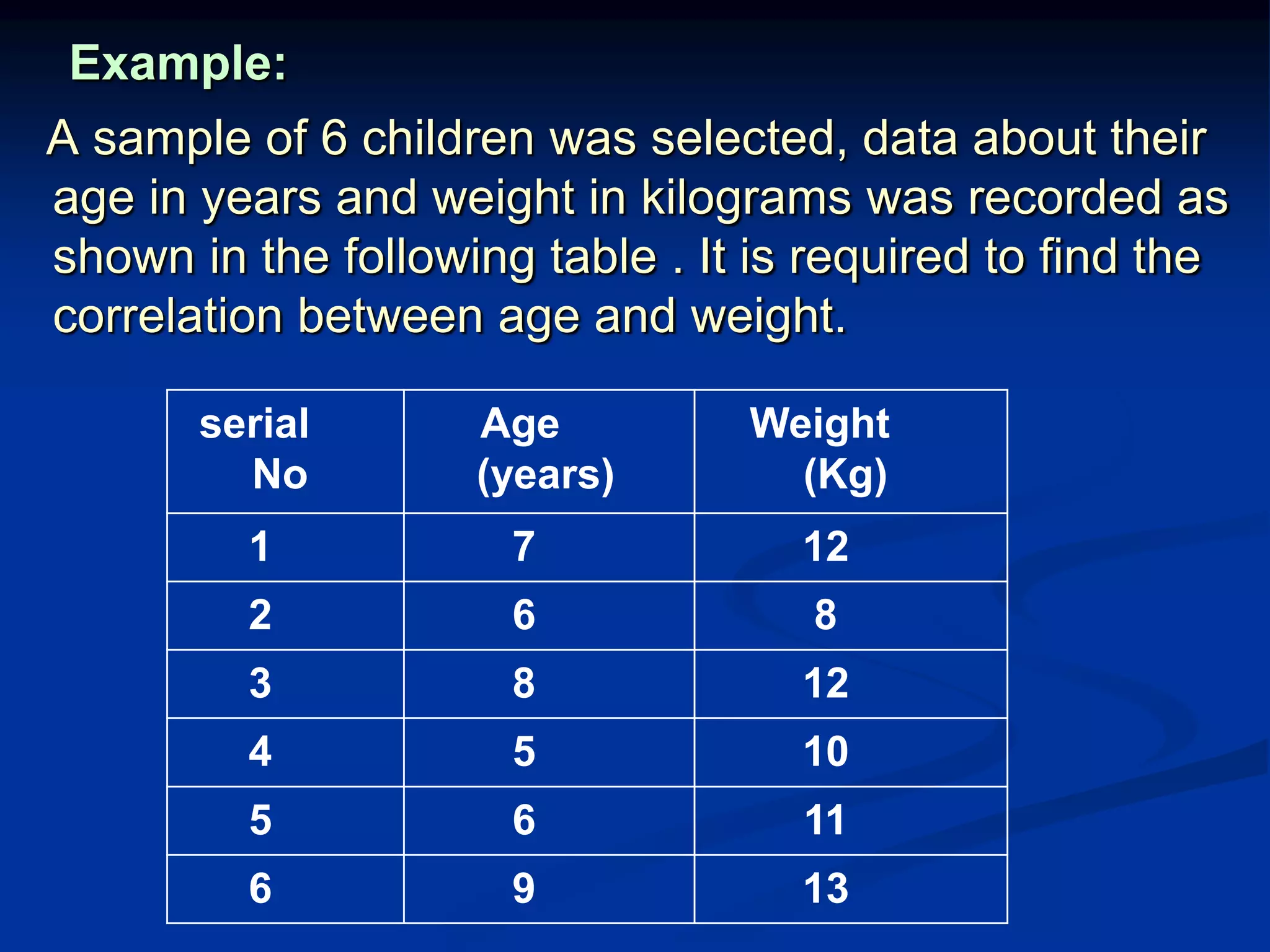
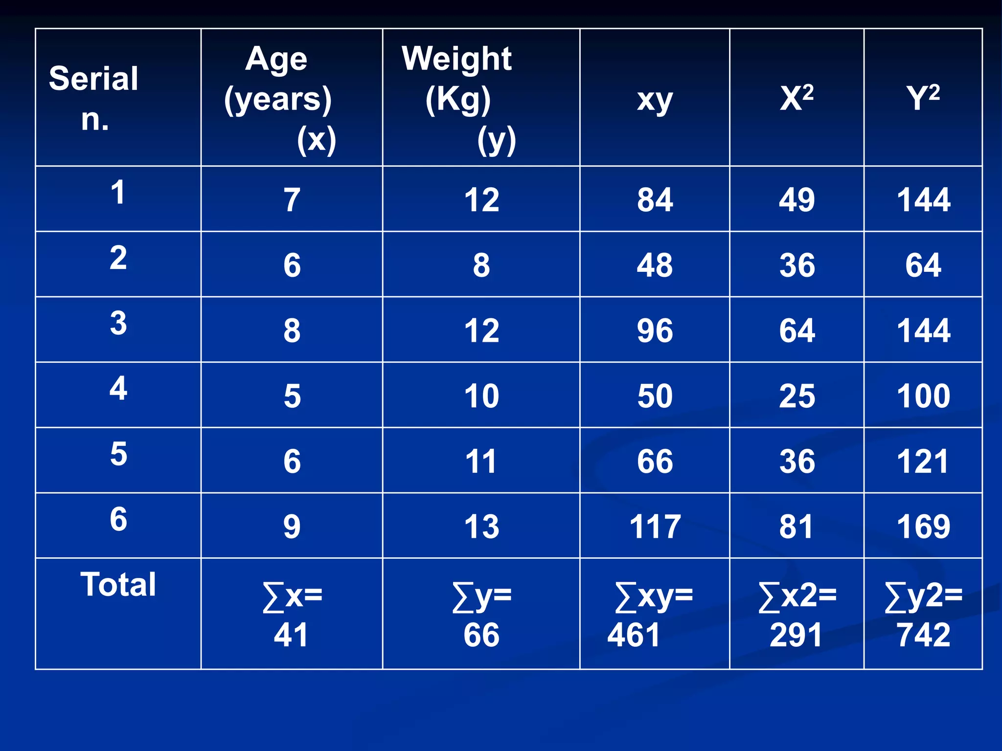
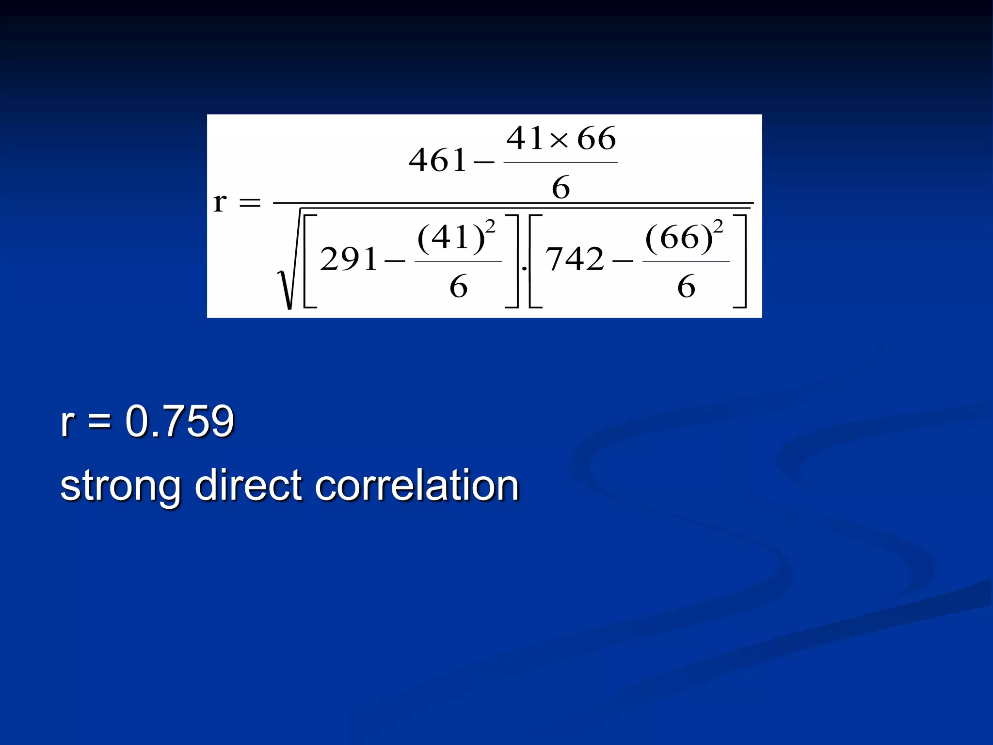
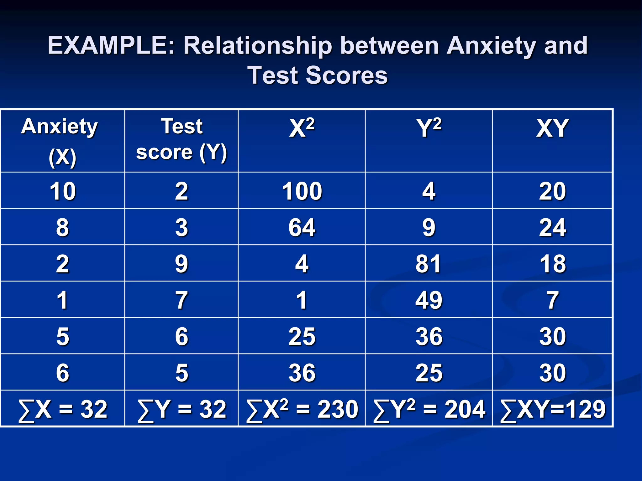
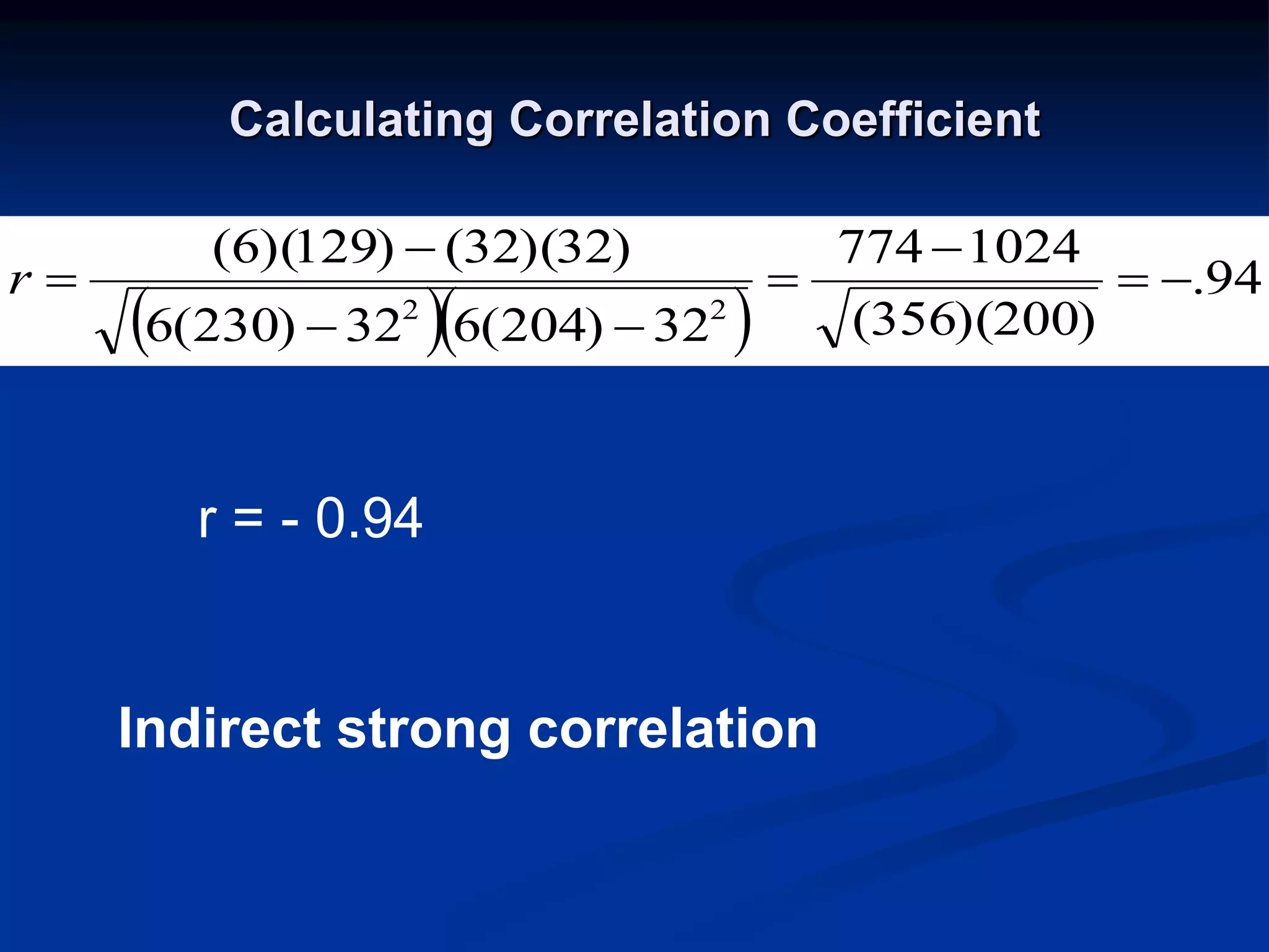
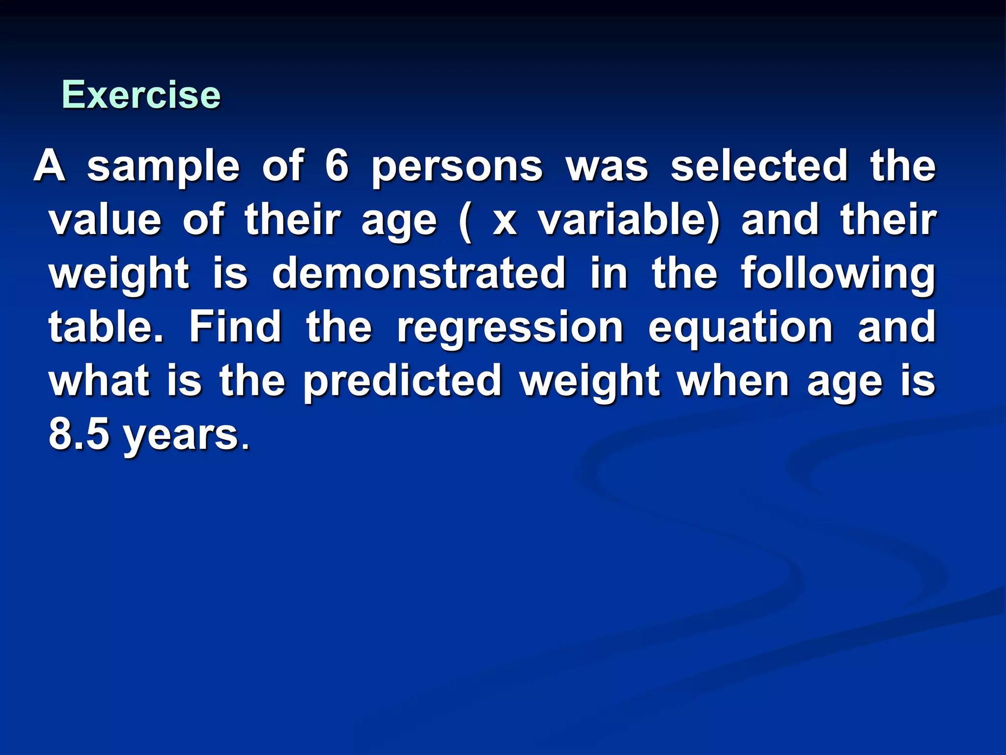
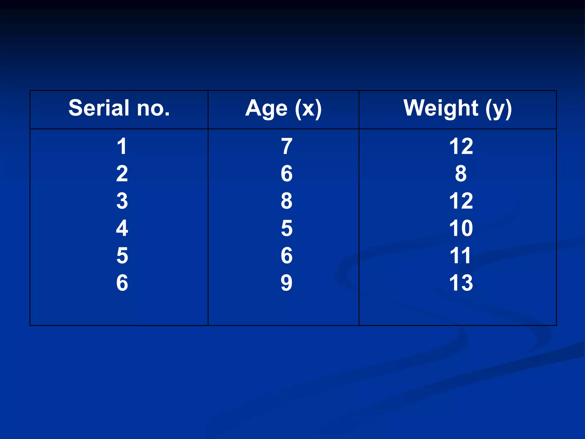
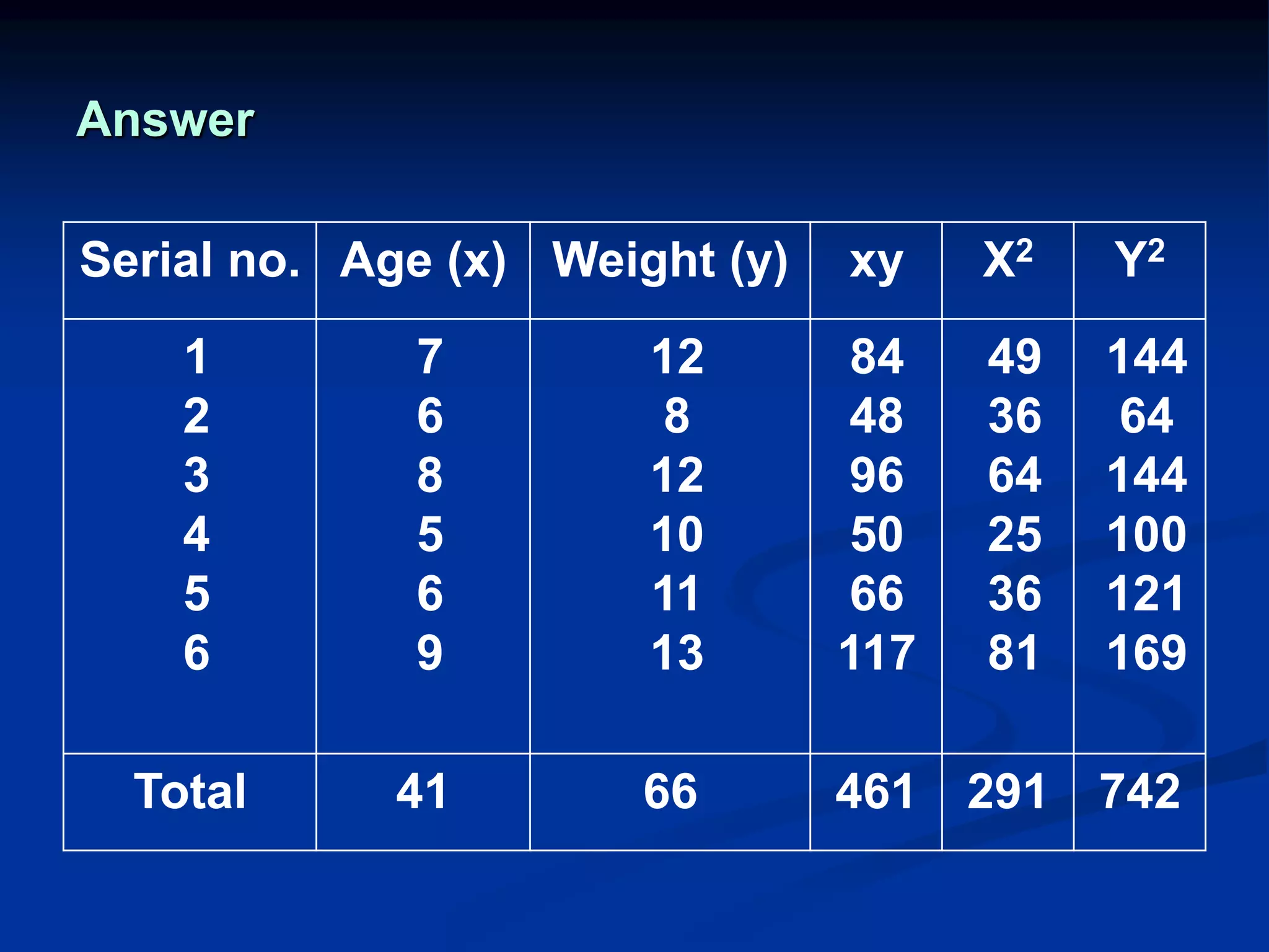
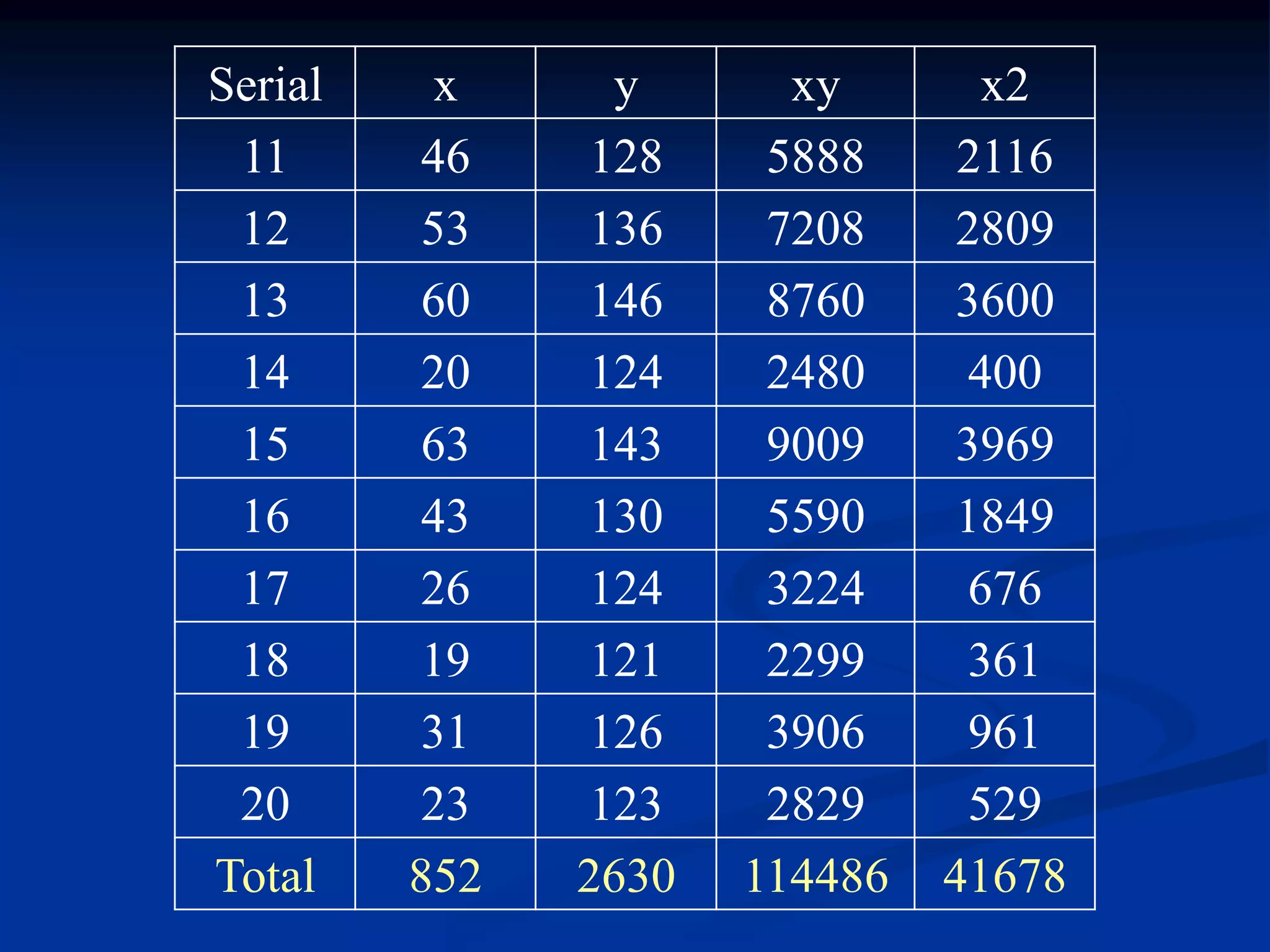
Examples of calculating correlation coefficients with data on age and weight, and anxiety with test scores.
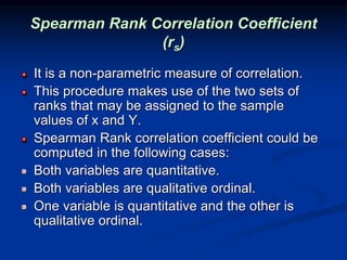
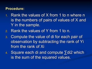
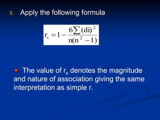
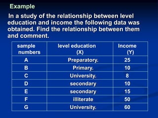
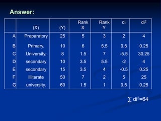
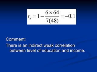
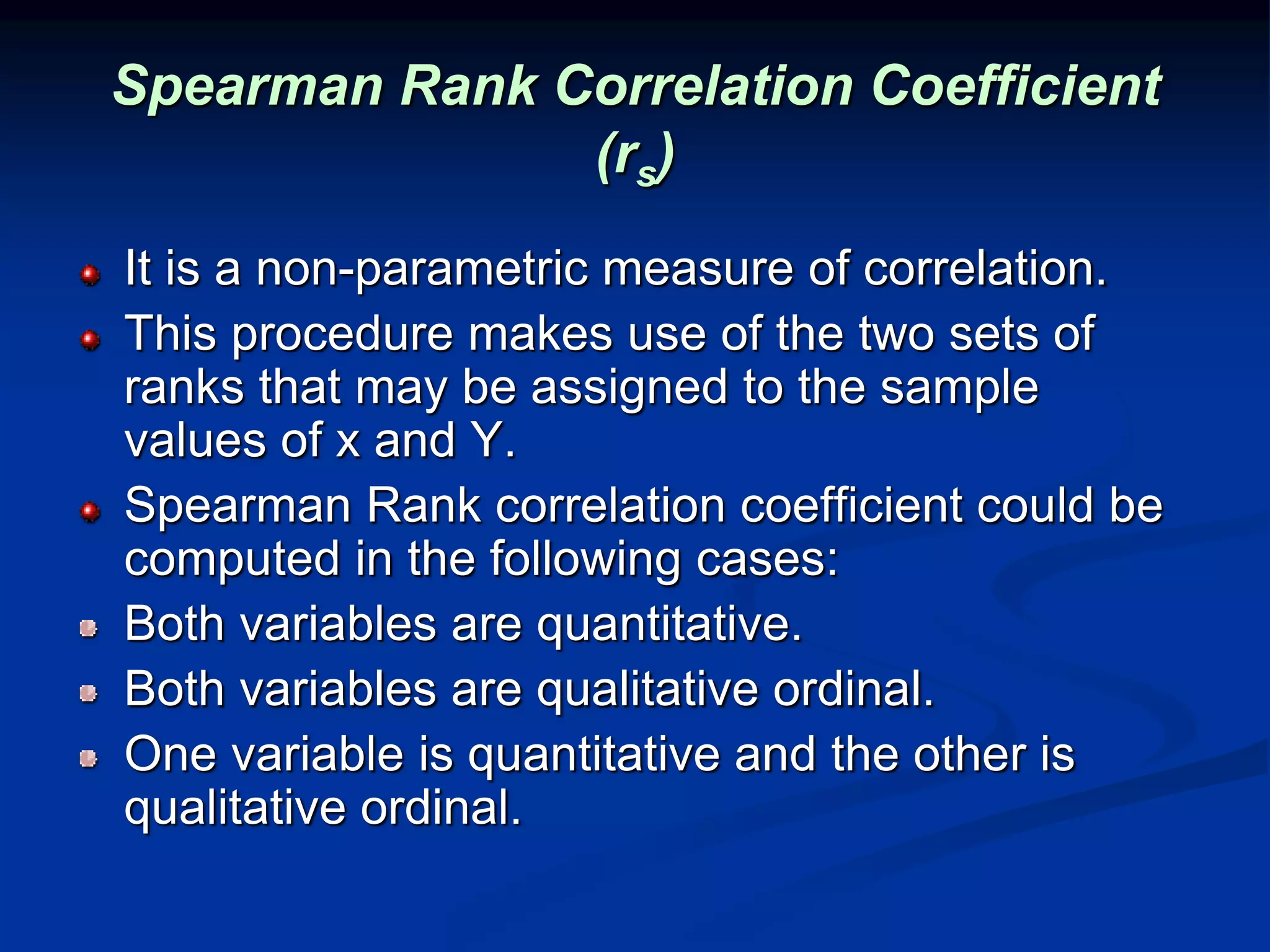
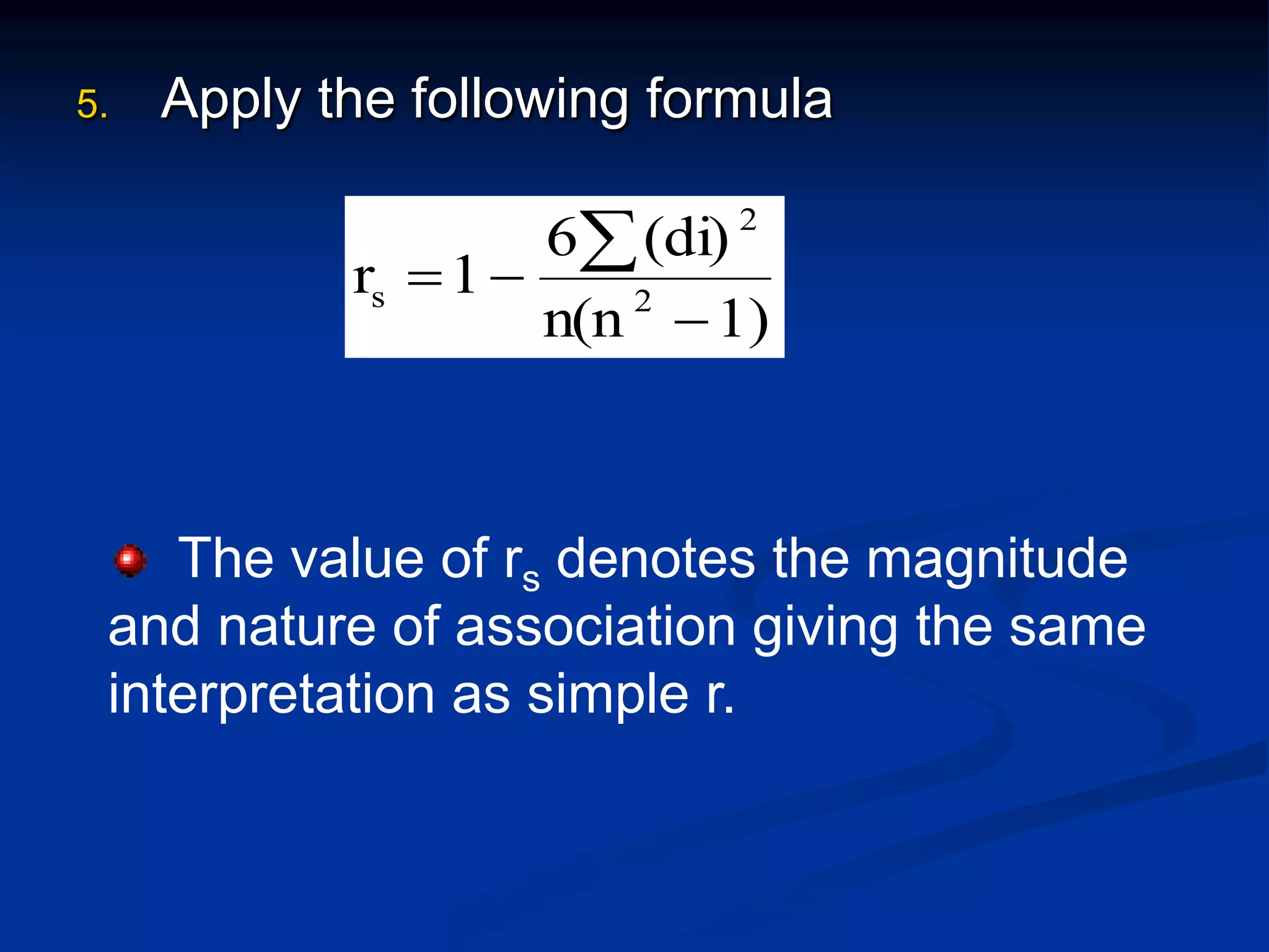
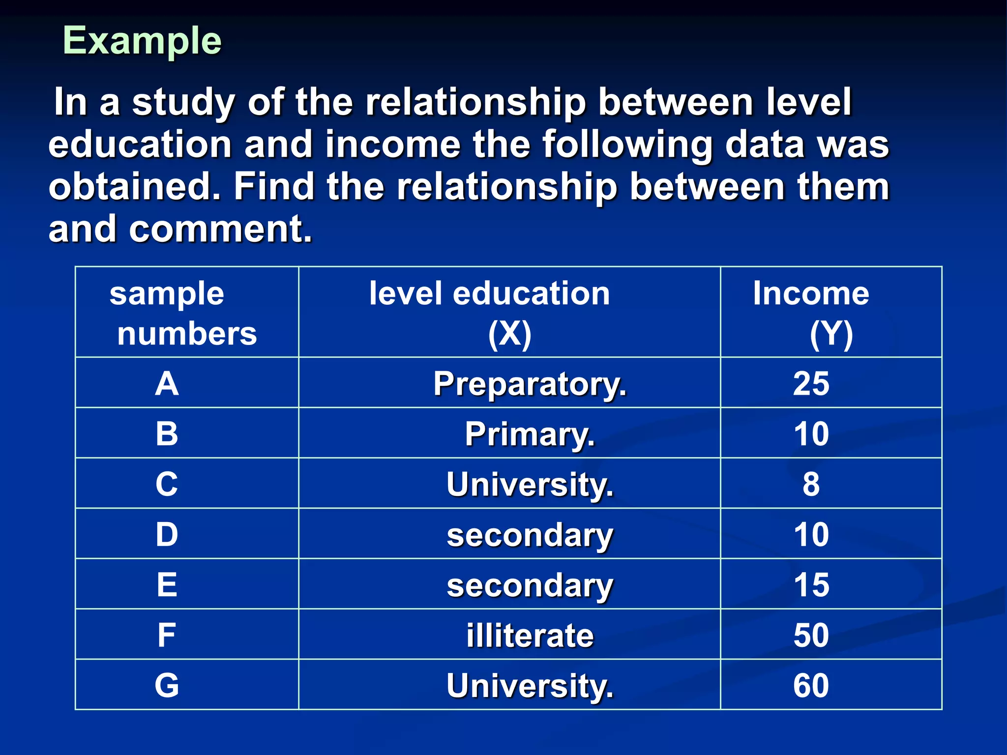
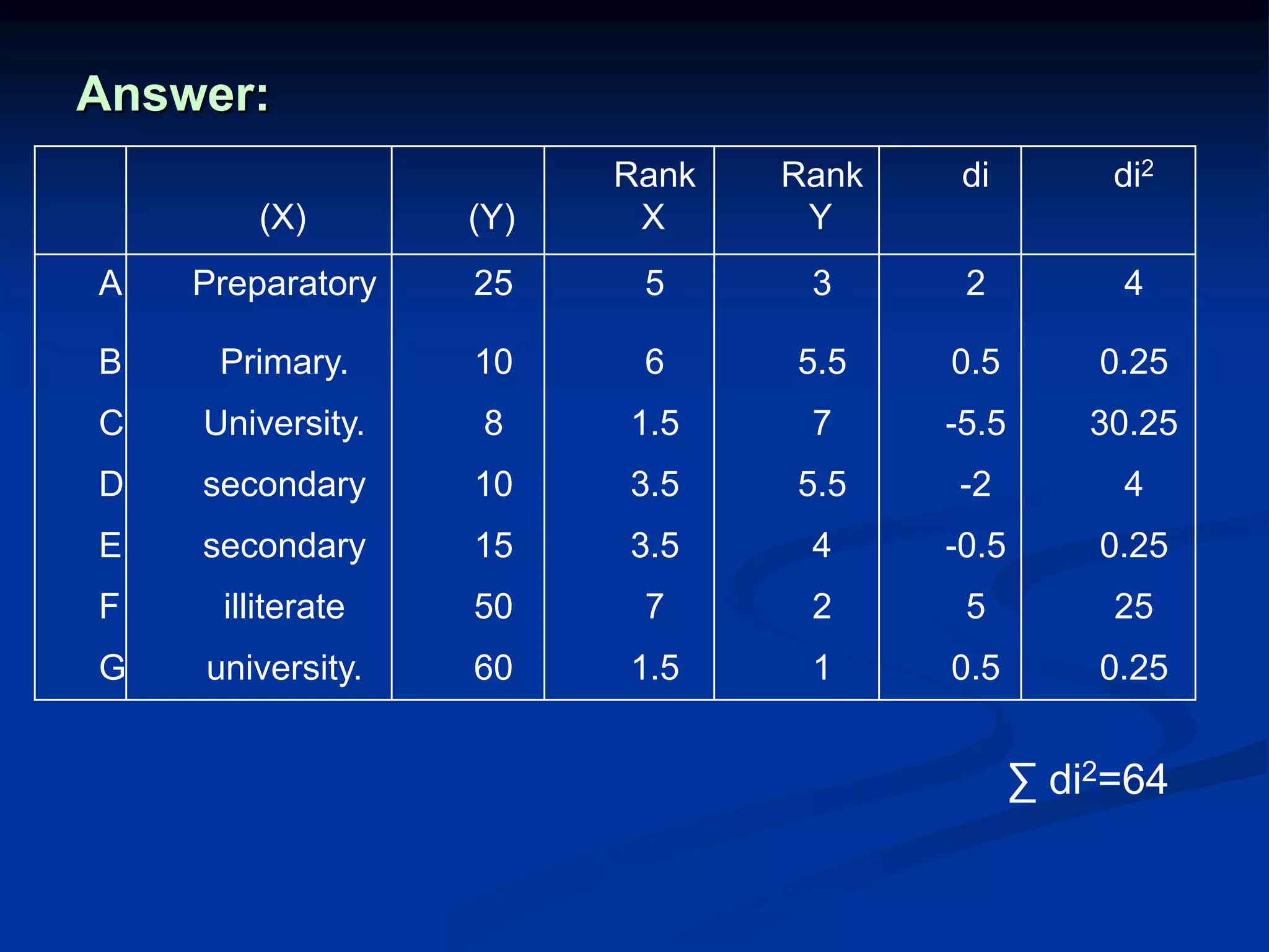
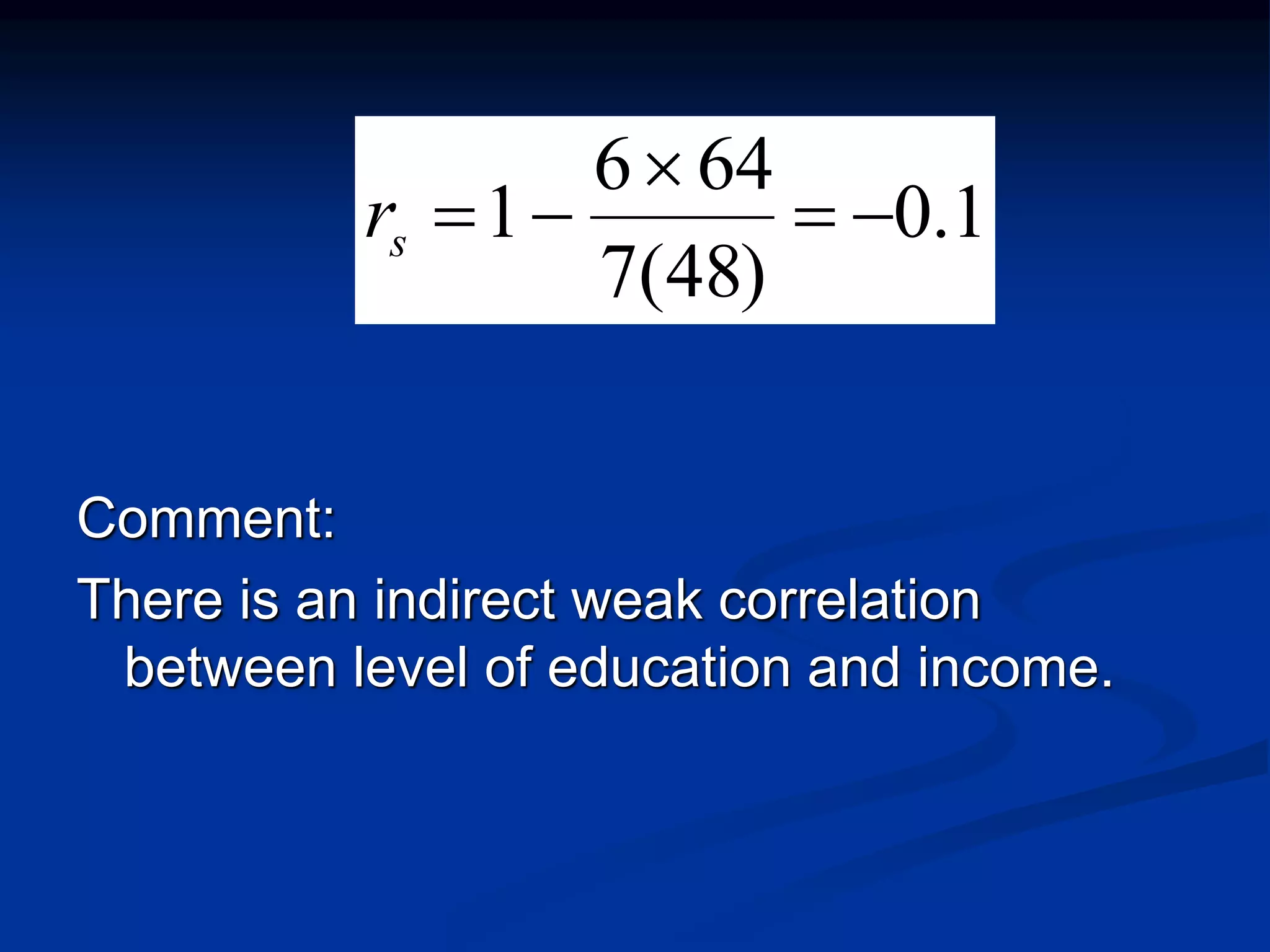
Introduces Spearman's rank correlation for ordinal data and provides an example with education and income.
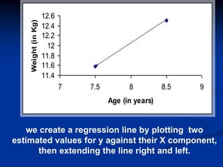
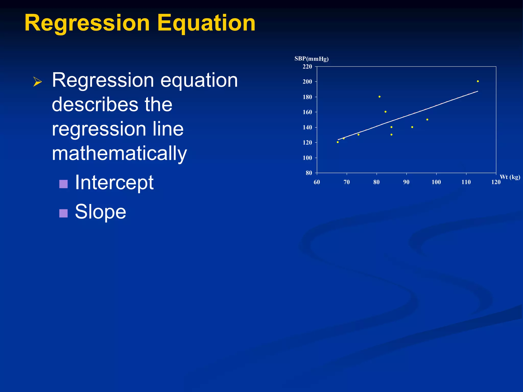
Explains regression and its purpose in predicting outcomes. Reinforces the connection between correlation and regression.
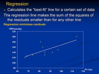
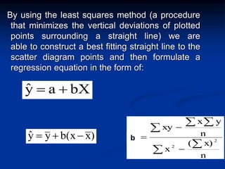
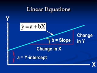
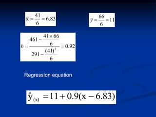
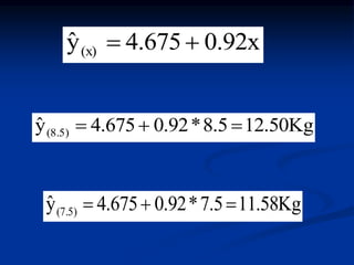
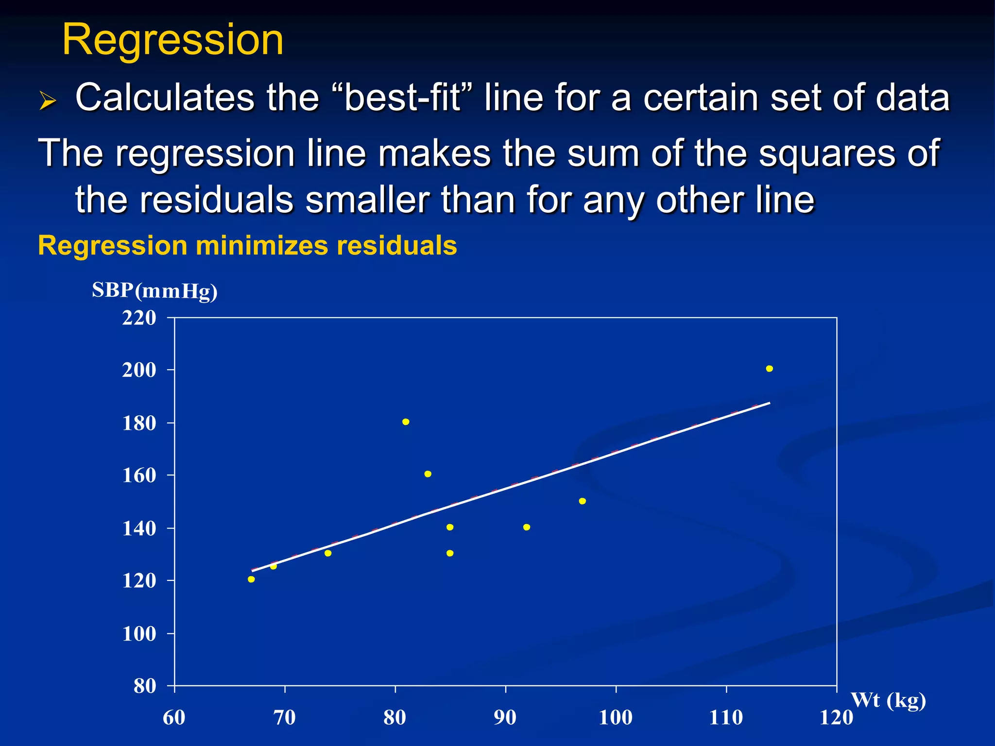
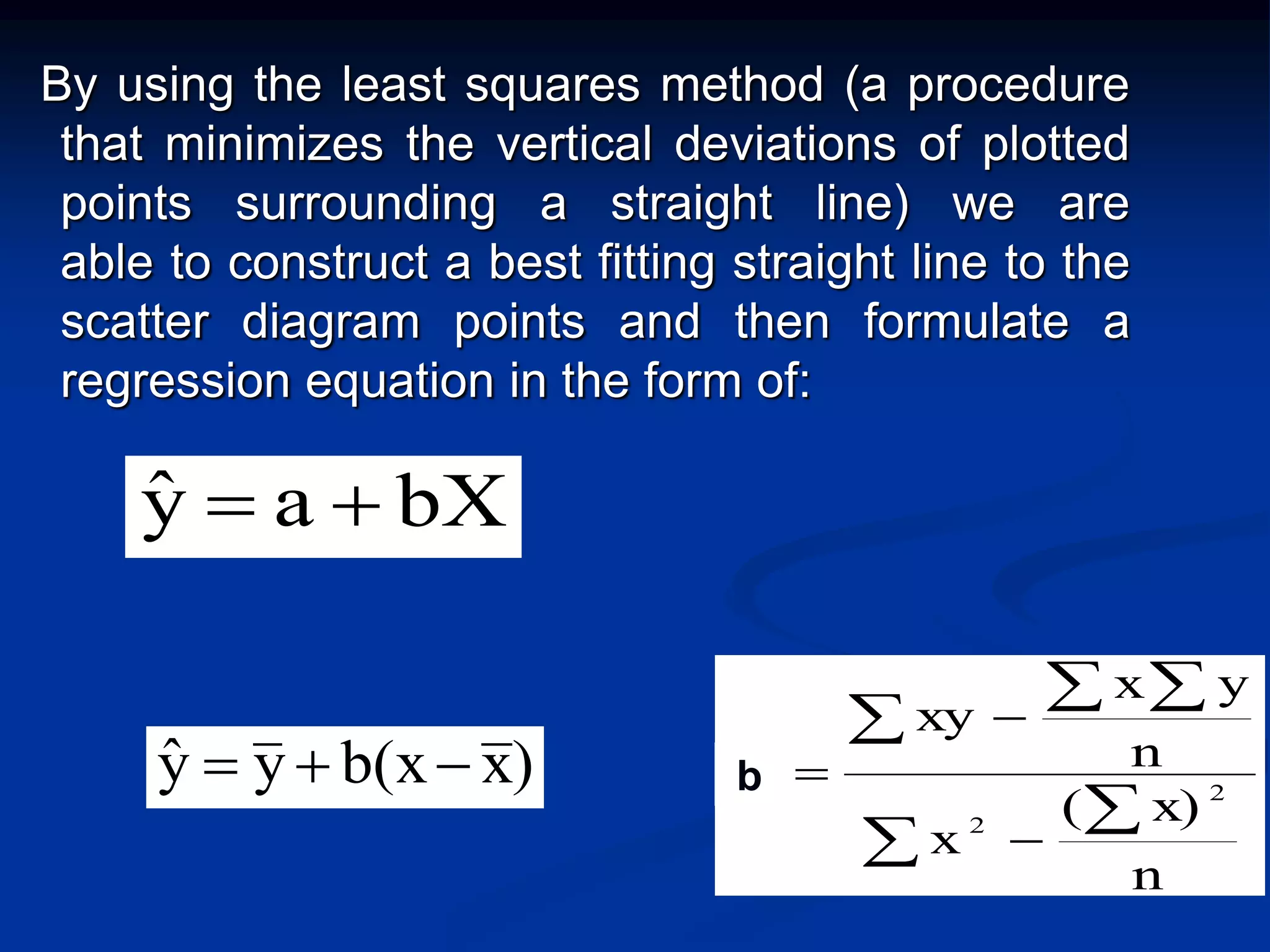
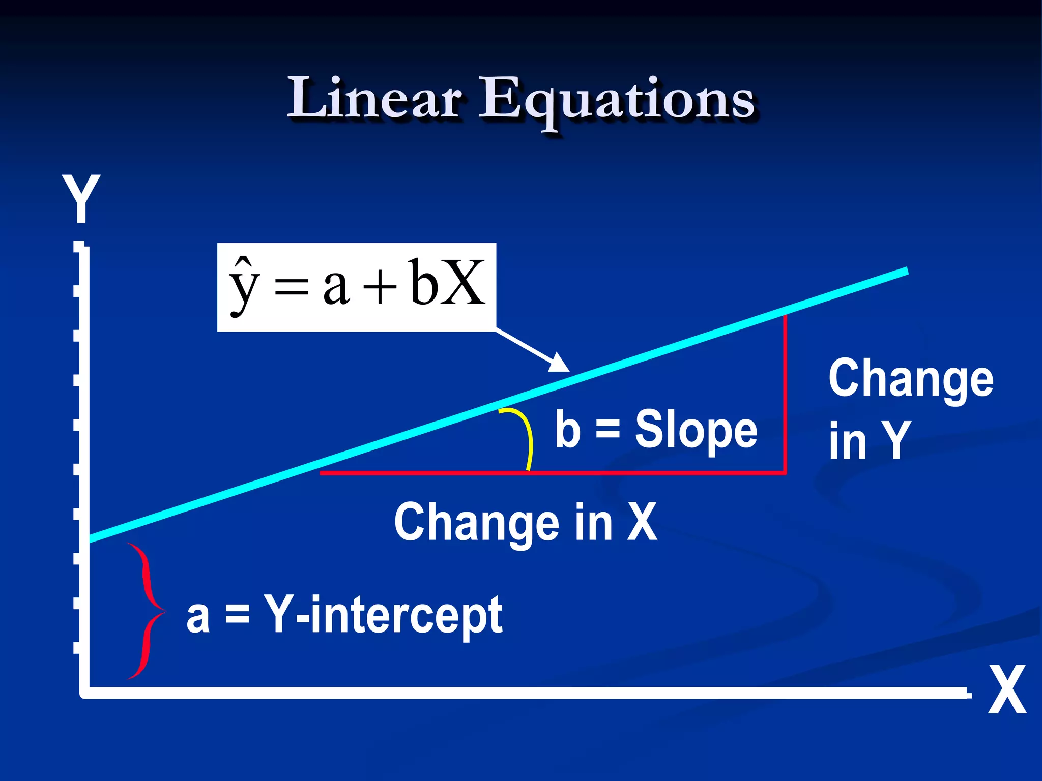
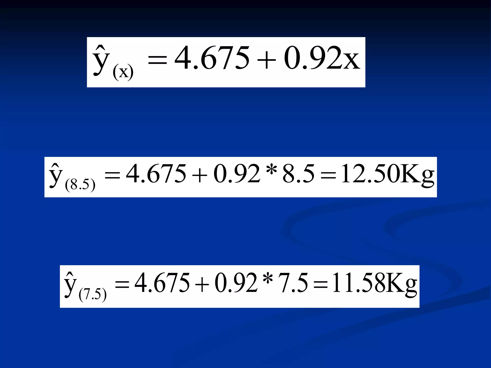
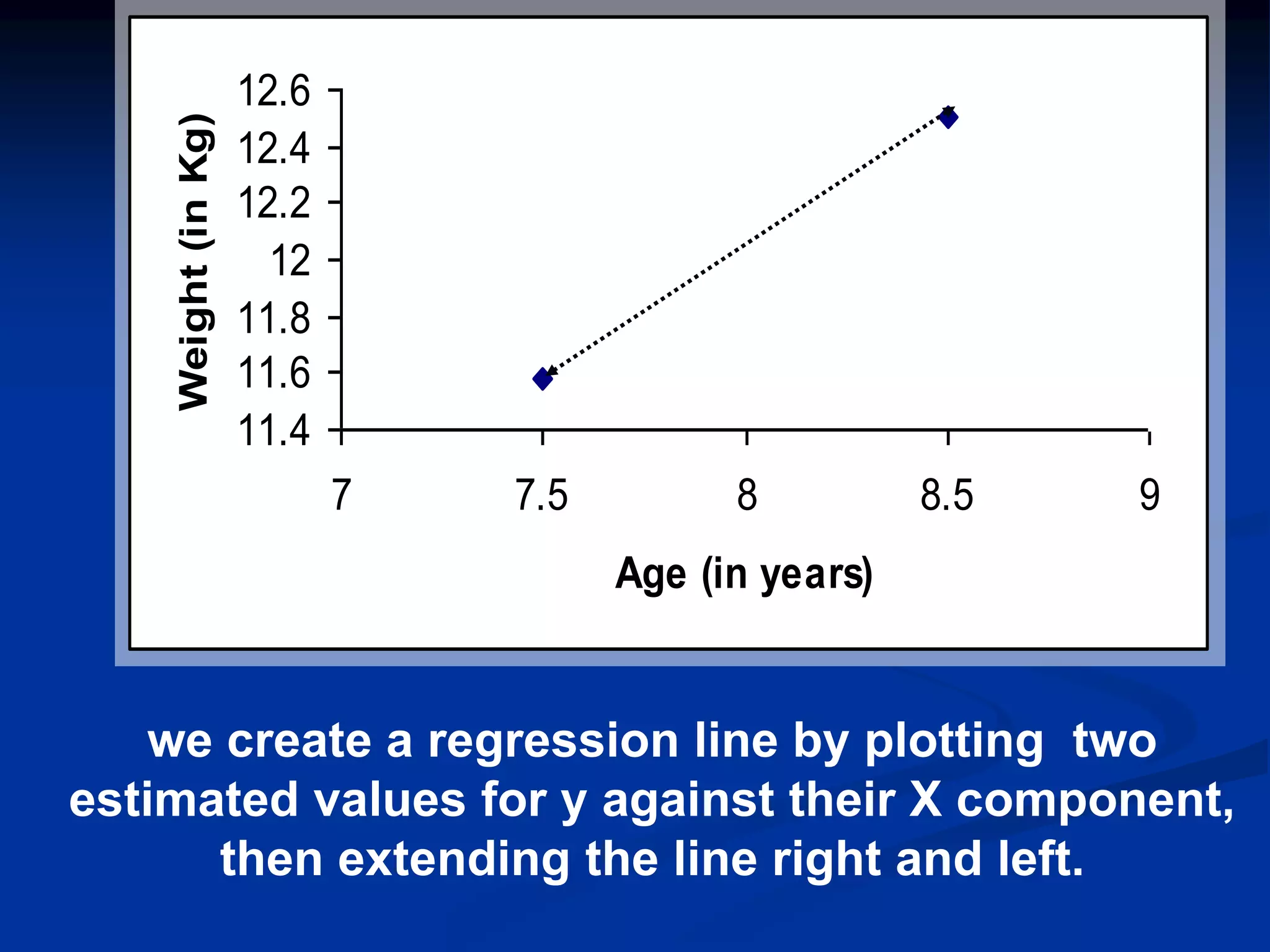
Describes the least squares method for deriving regression lines and equations to predict variable changes.
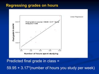
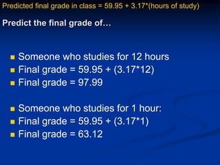
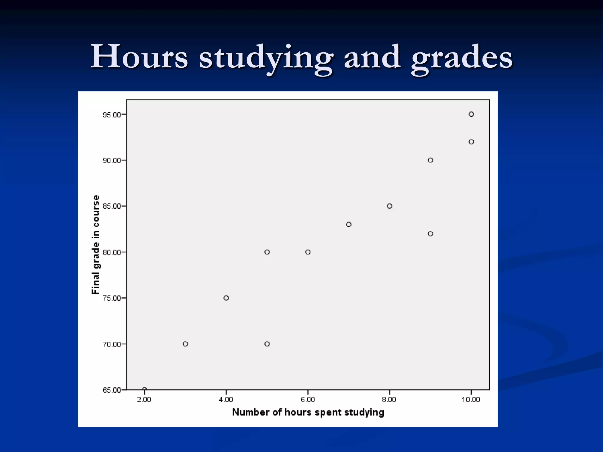
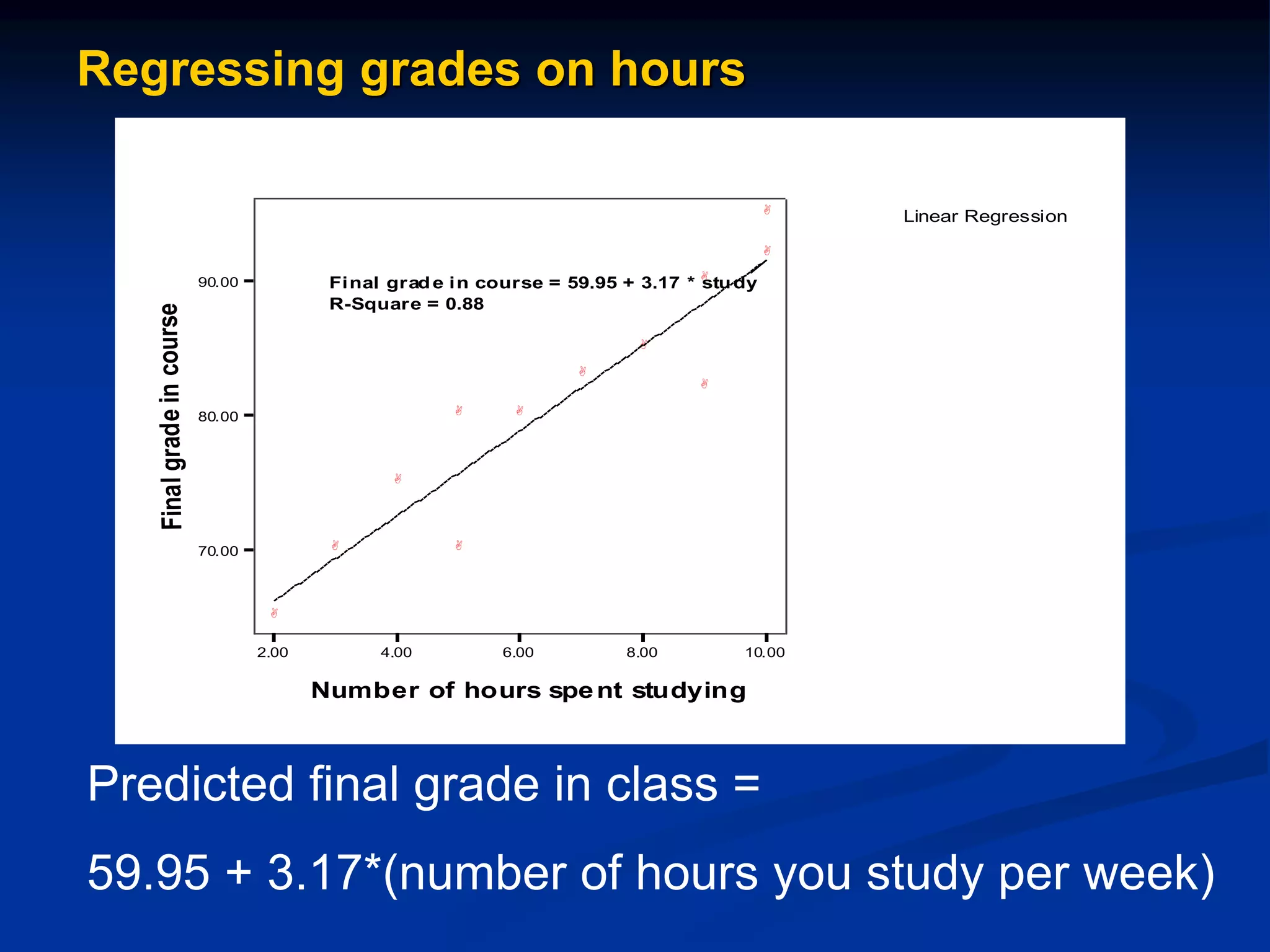
Practical example of predicting final grades based on study hours with regression equations.
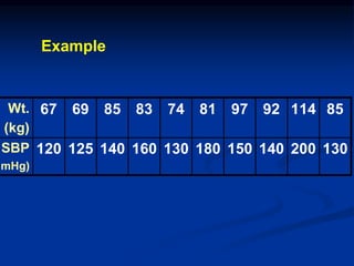
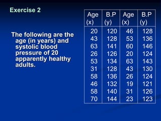
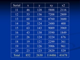
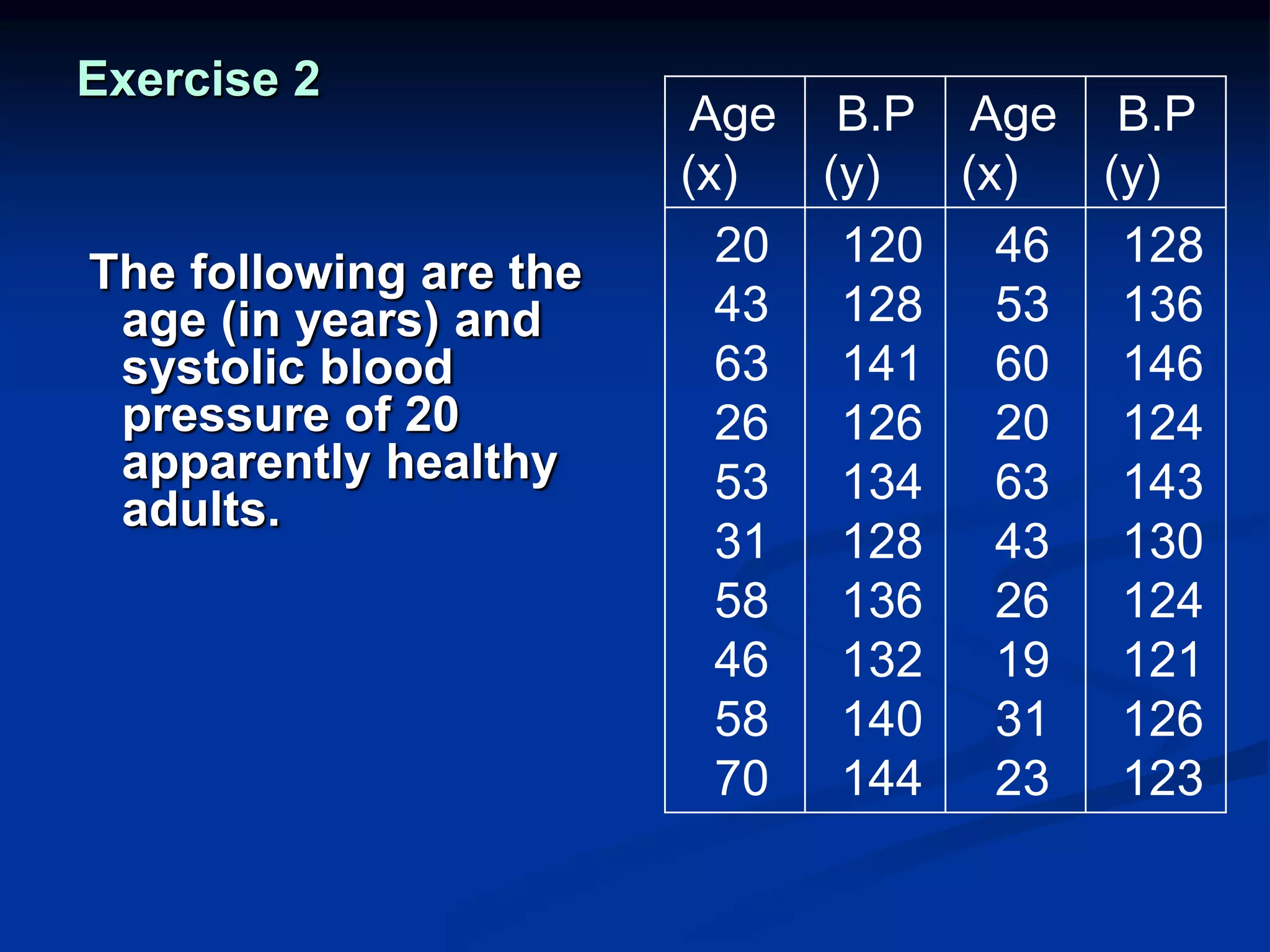
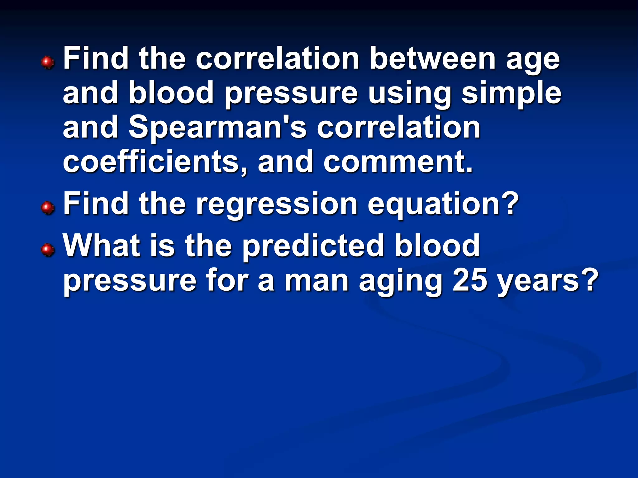
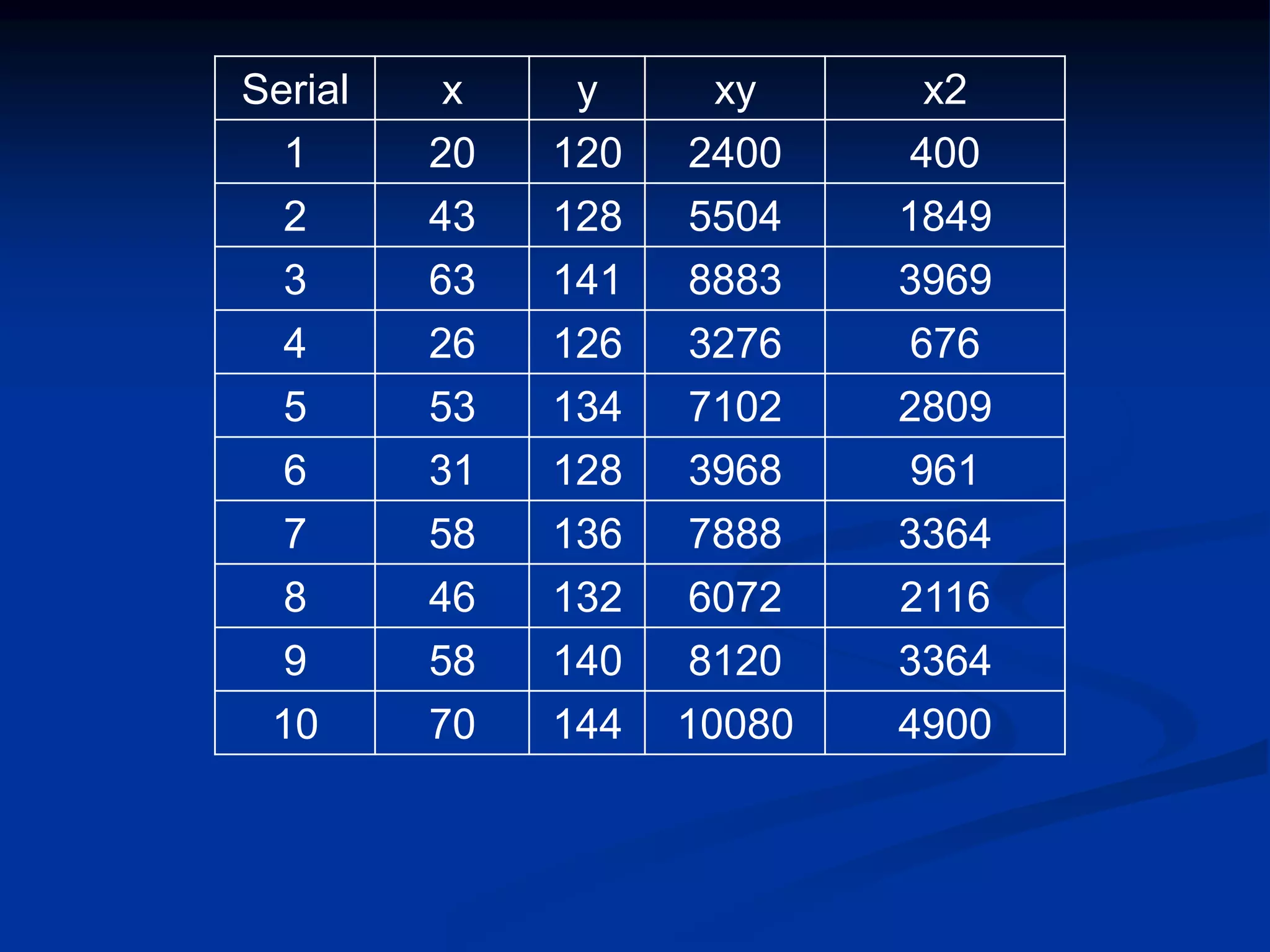
Assessment of relationships between age and blood pressure, including correlation and regression calculations.


