


This document provides an overview of regression models and analysis techniques. It introduces simple and multiple linear regression, as well as logistic regression. It discusses assessing regression models, cross-validation, model selection, and using regression models for prediction. Additionally, it covers the similarities and differences between linear and logistic regression, and assessing correlation without inferring causation. Scatter plots, correlation coefficients, and computing regression equations are also summarized.
Introduction to Regression Models, including simple and multiple linear regression, logistic regression, assessing models, and prediction.
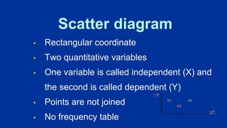
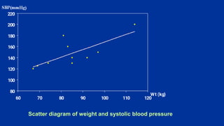
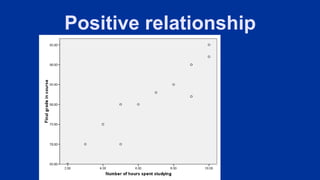
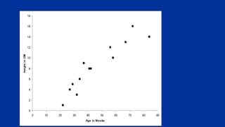
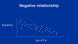
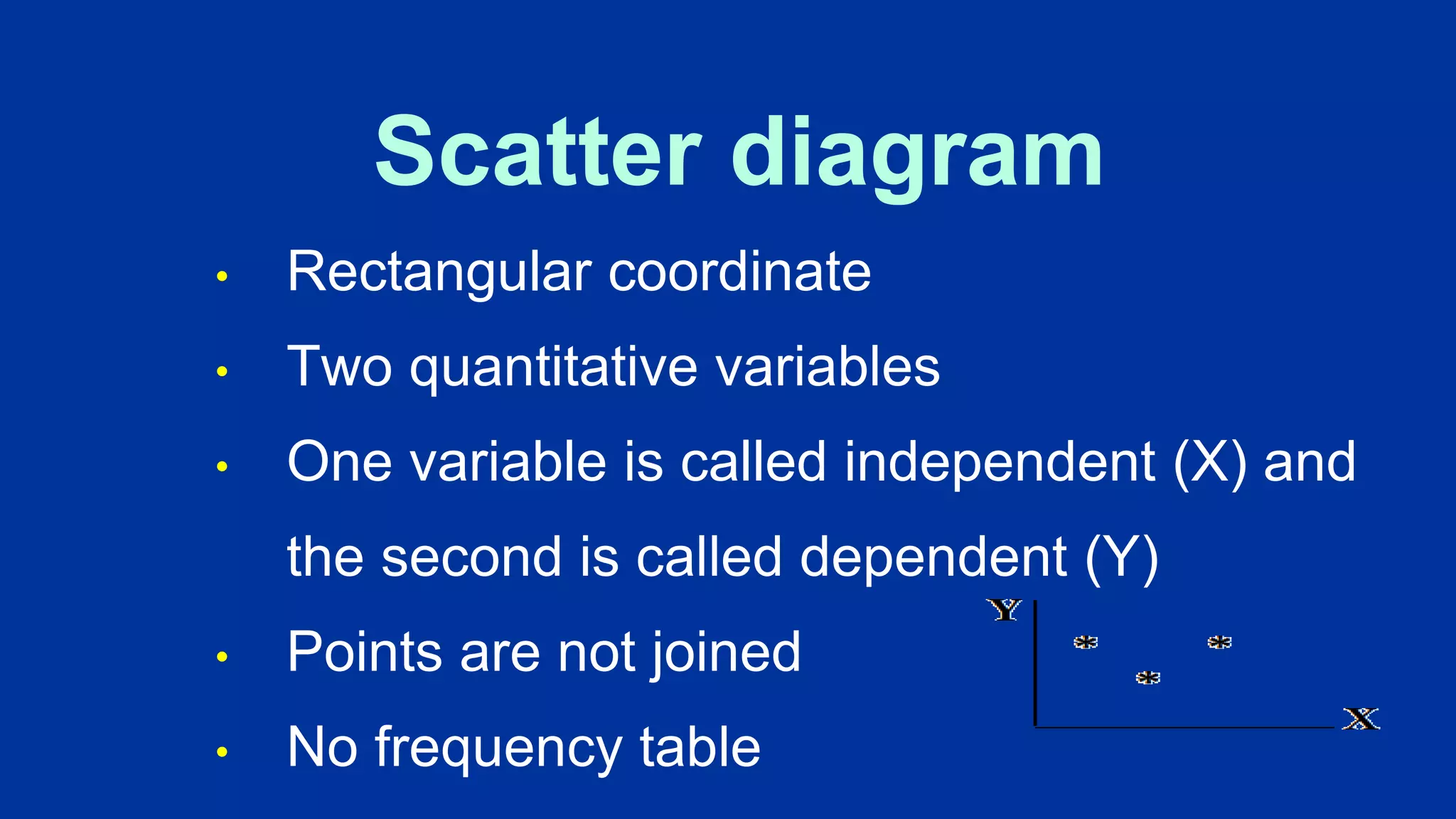
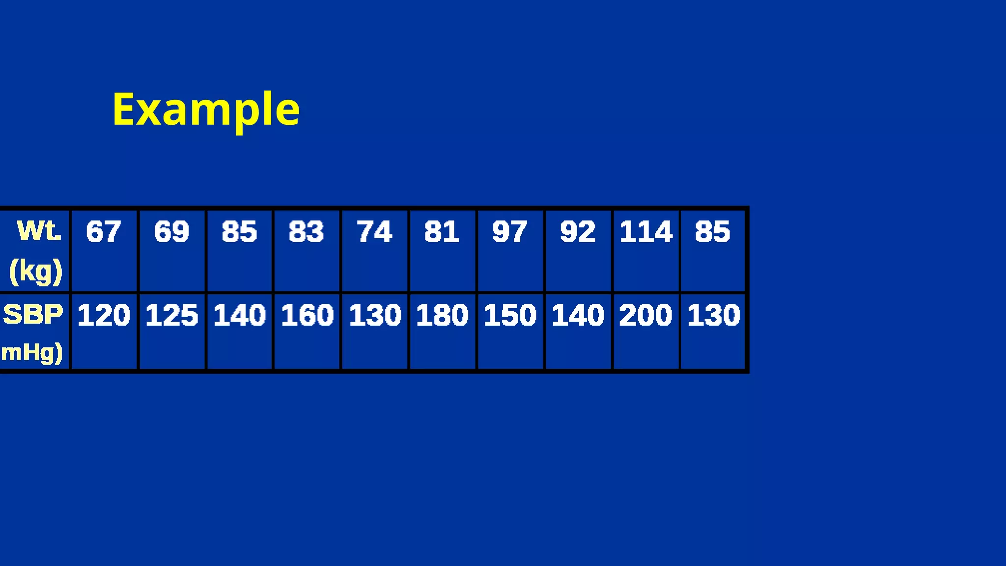
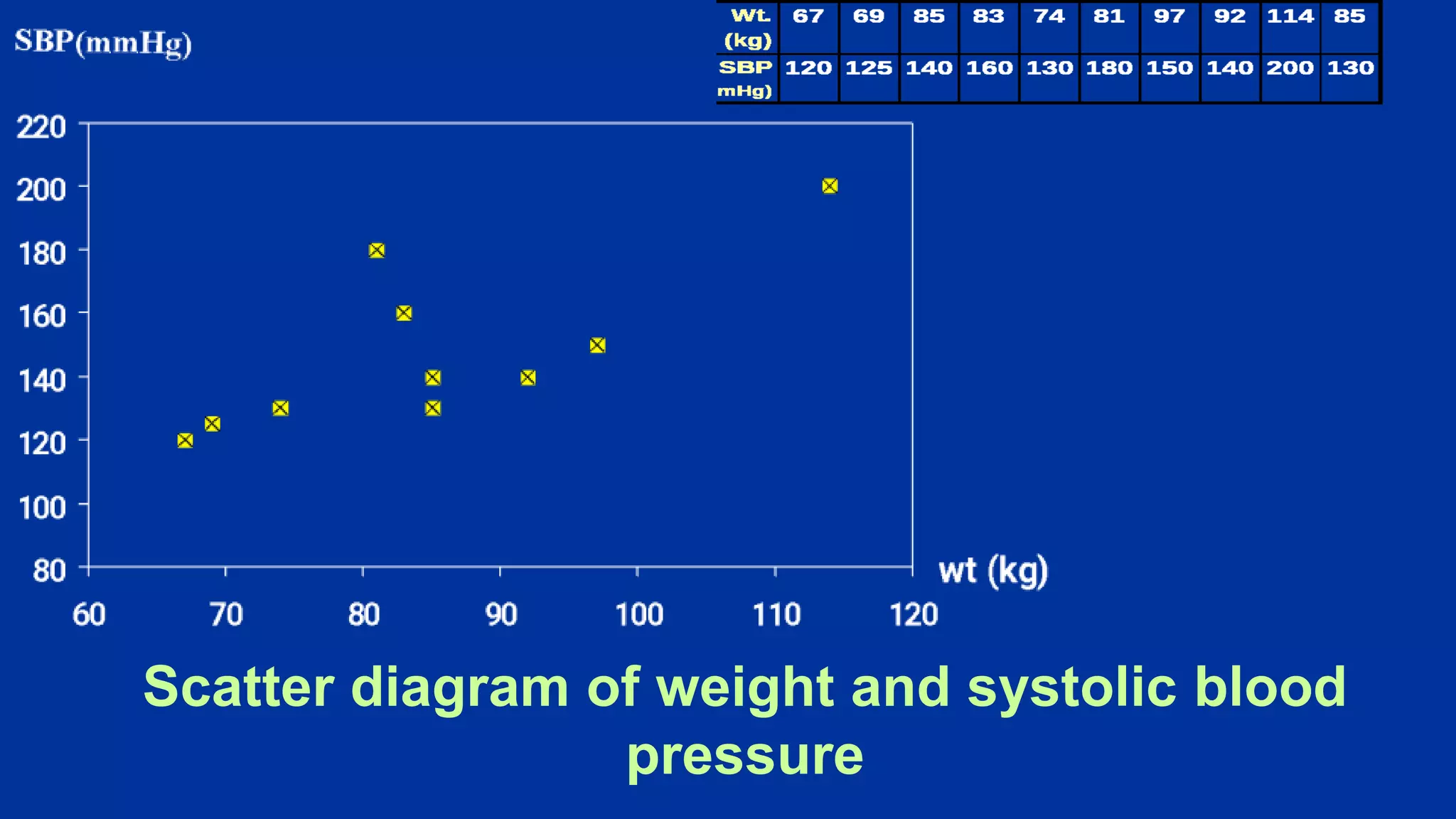
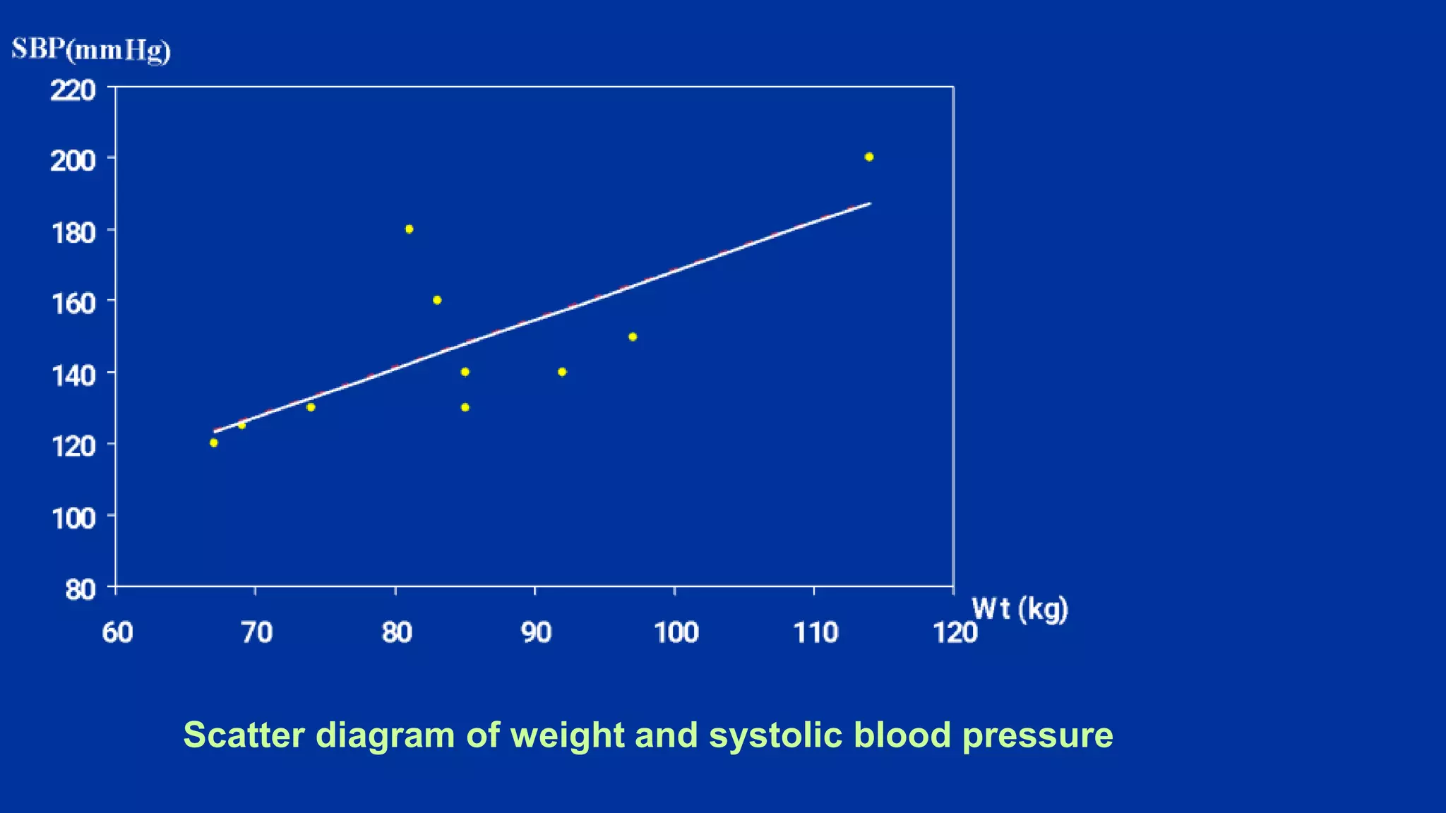
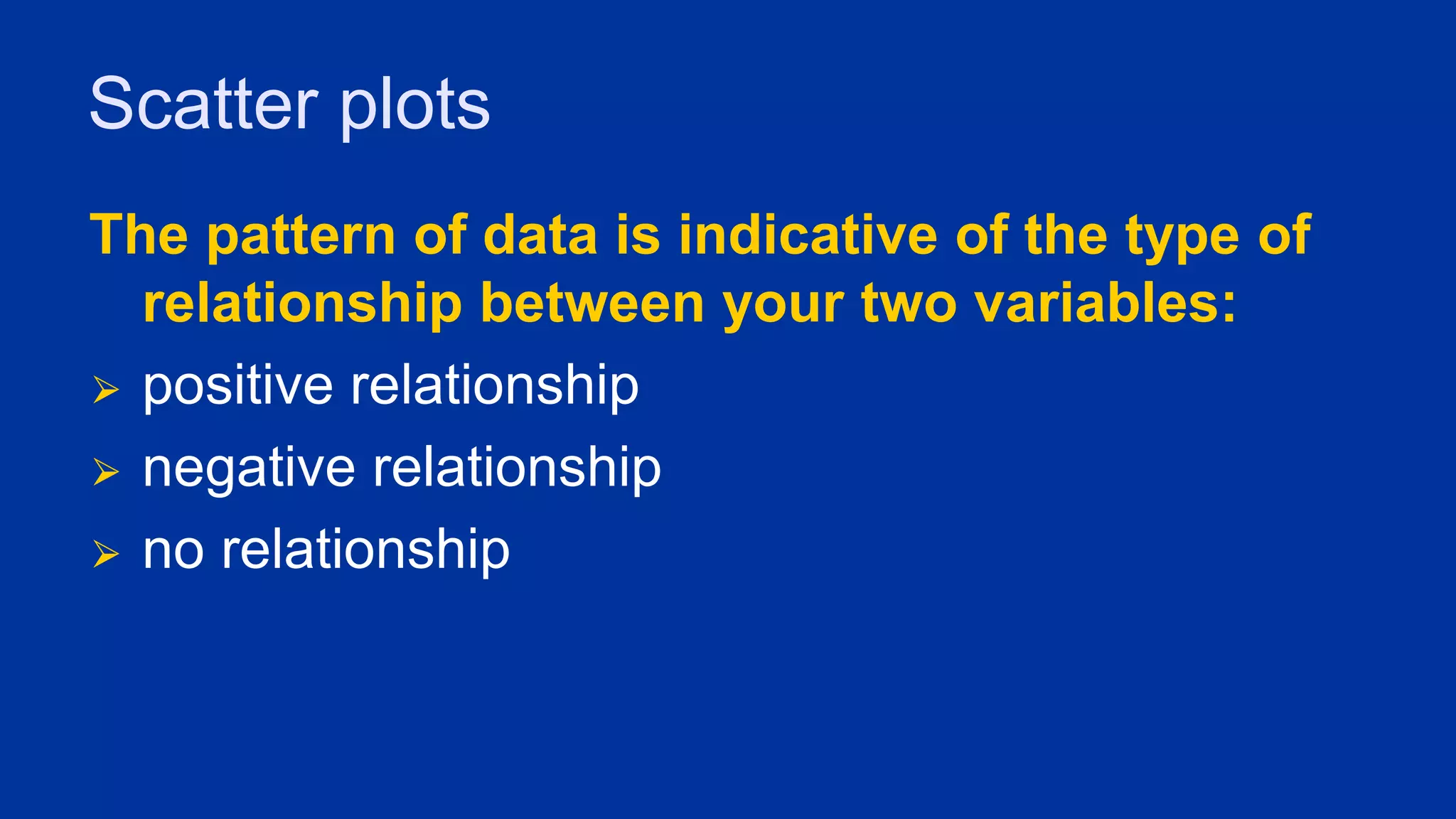
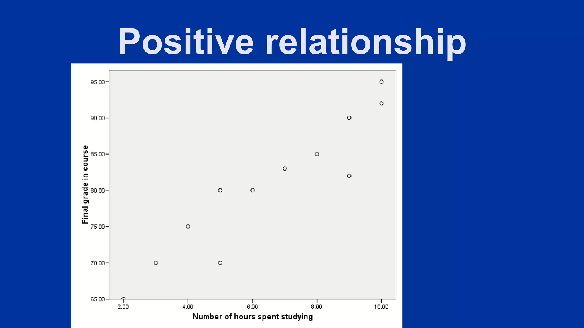
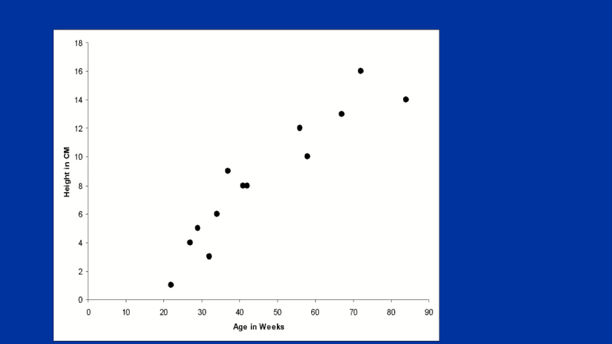
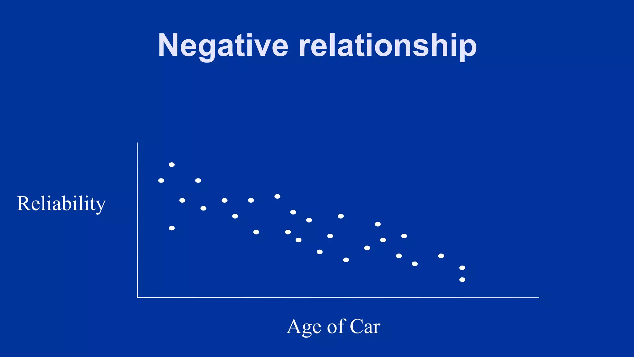
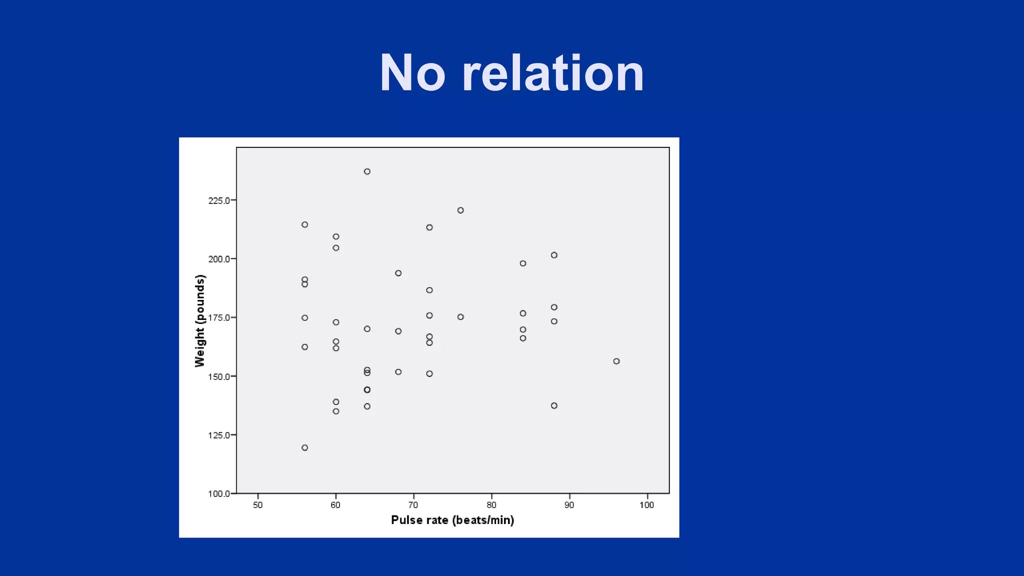
Definition of correlation, types of relationships between quantitative variables, illustrated with scatter diagrams.
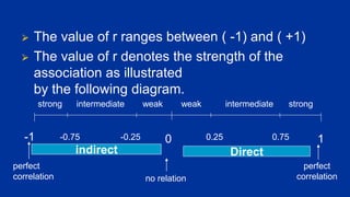
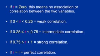
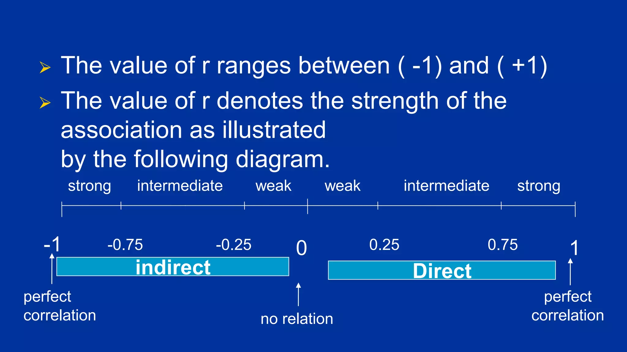
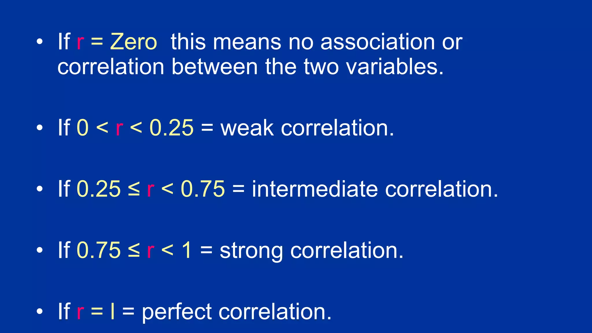
Explanation of correlation coefficient (r), its values, significance, and interpretation of relationships between variables.
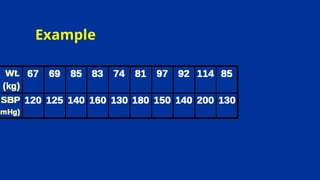
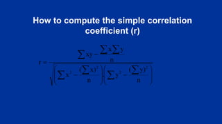
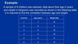
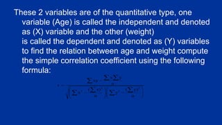
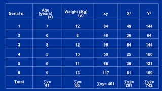
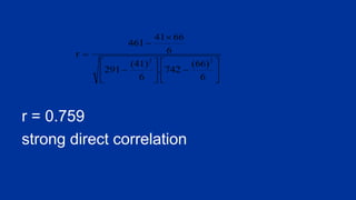
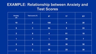
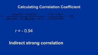
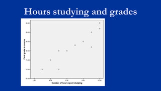
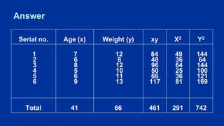
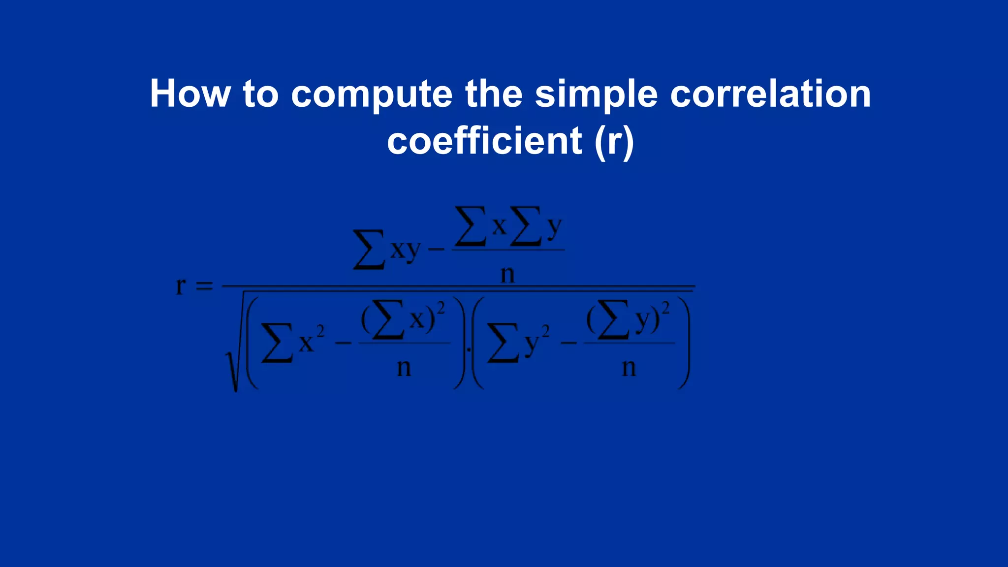
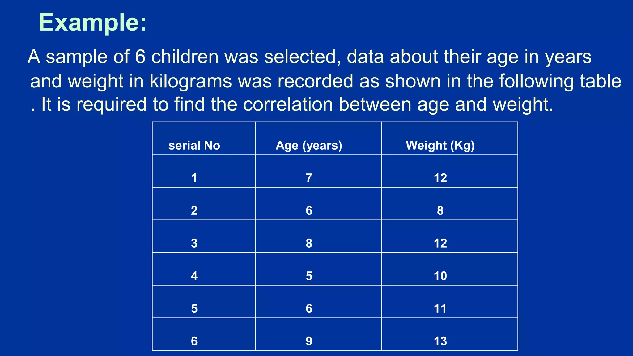
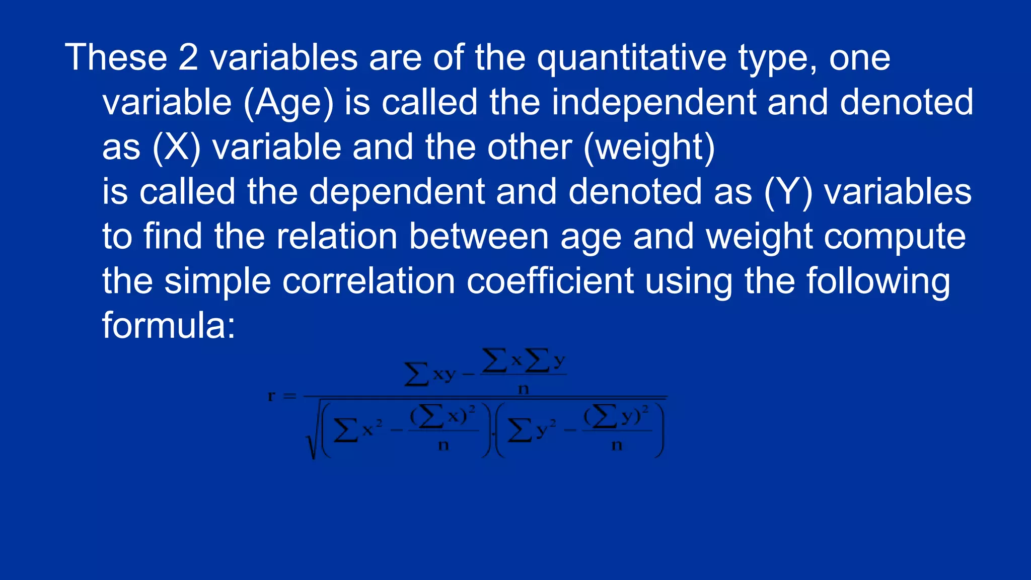
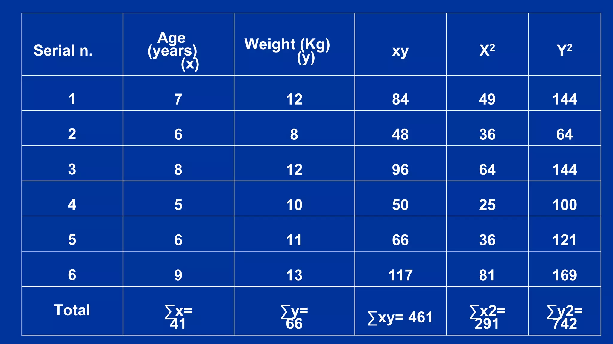
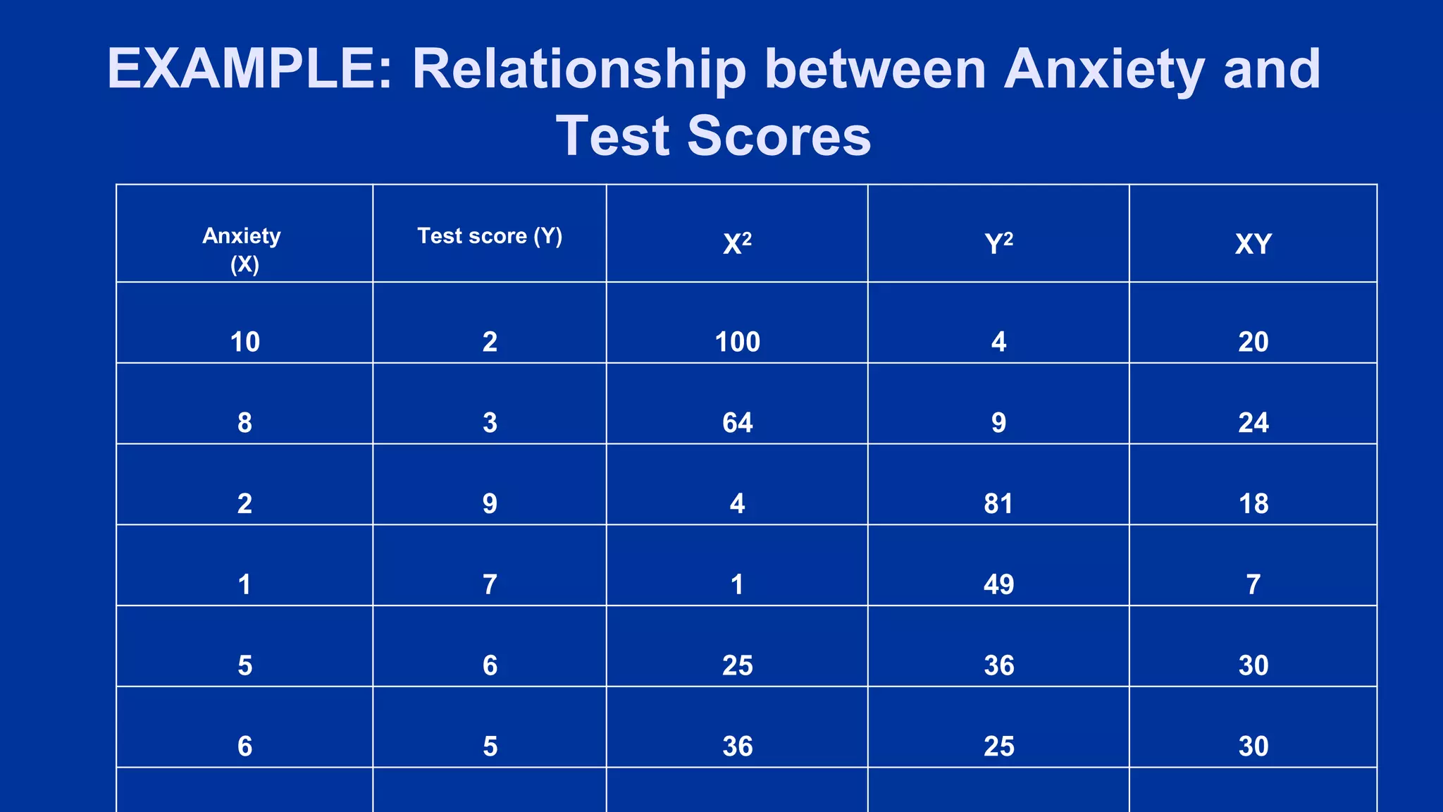
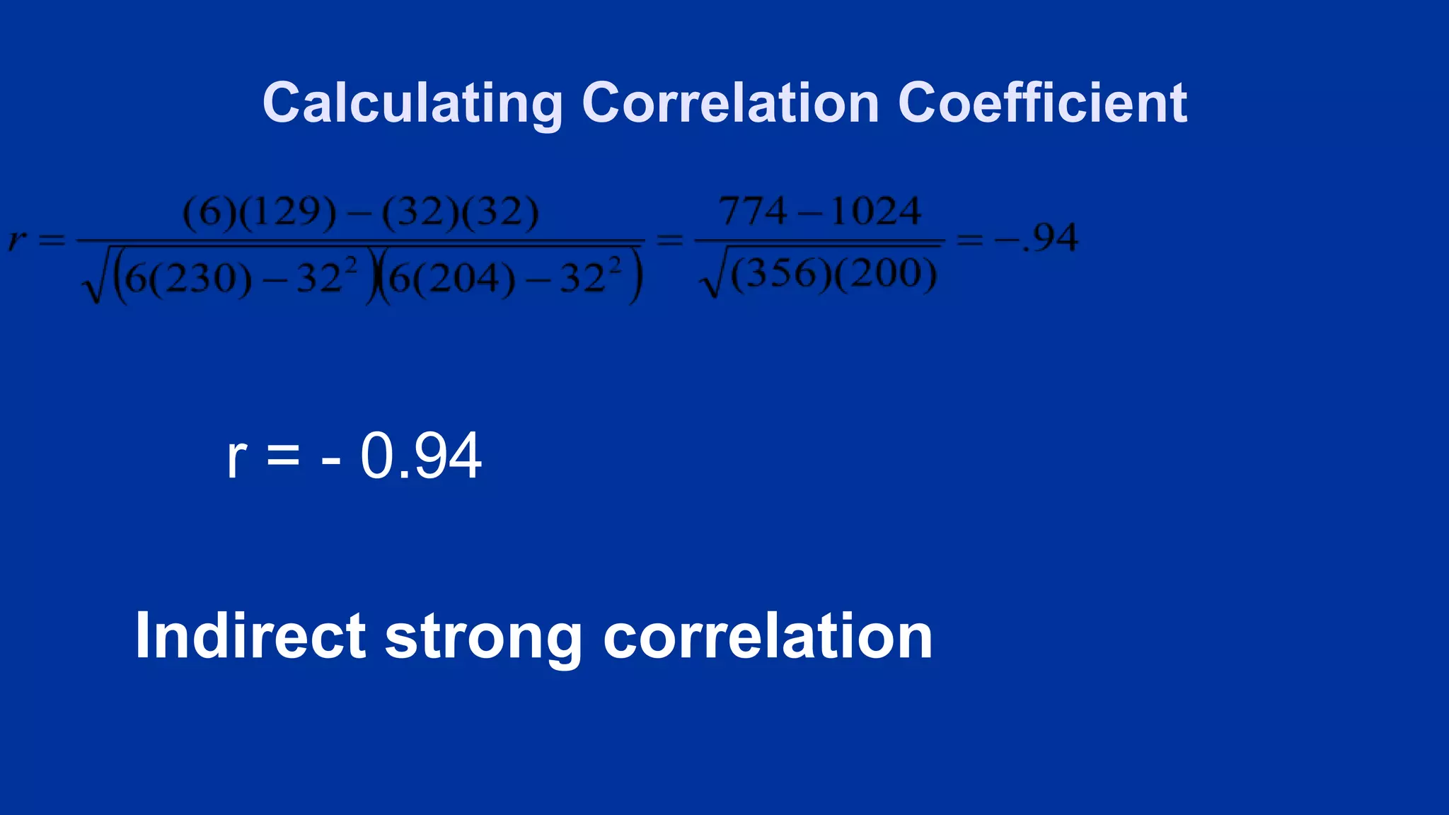
Calculating simple correlation coefficient using age and weight data, and analyzing anxiety and test scores relationship.
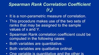
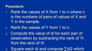
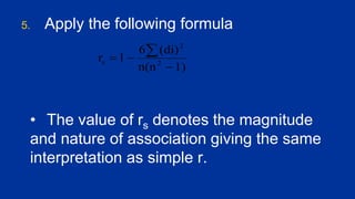
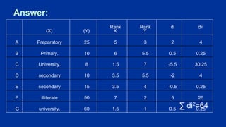
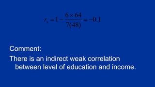
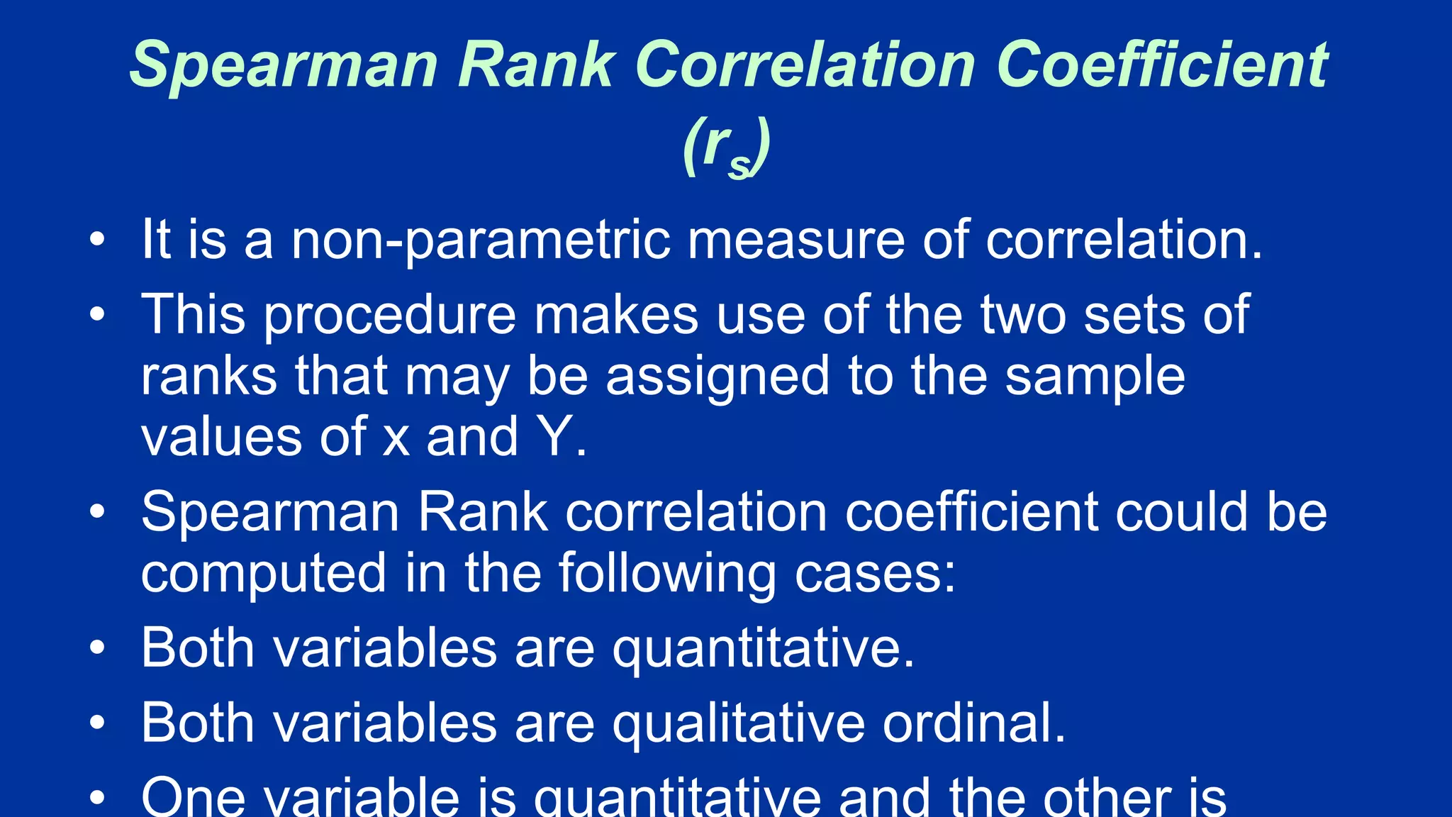
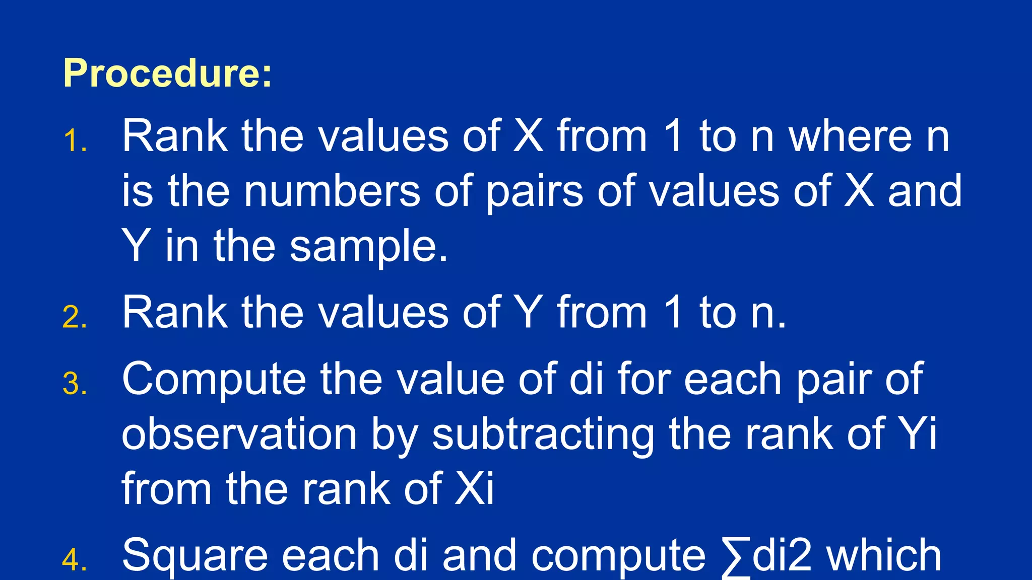
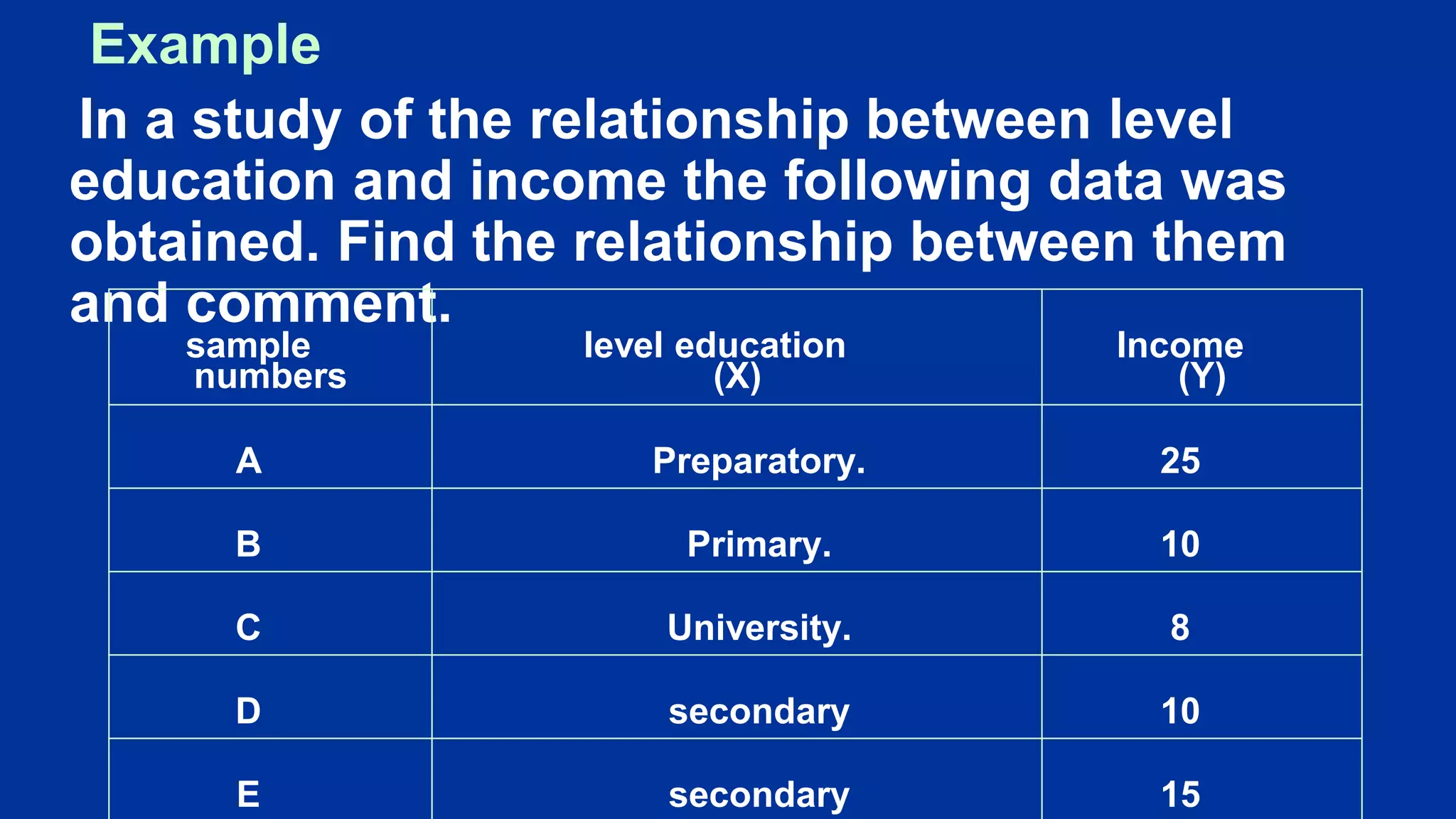
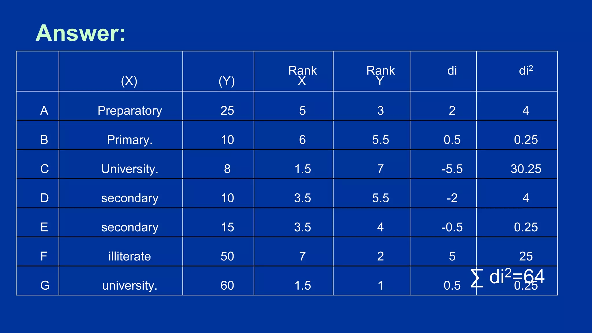
Spearman Rank Correlation Coefficient calculation process for both quantitative and ordinal qualitative variables.
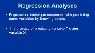
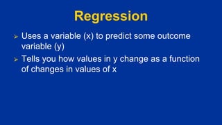
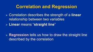
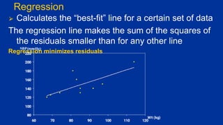
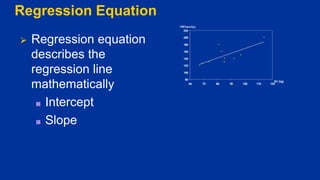
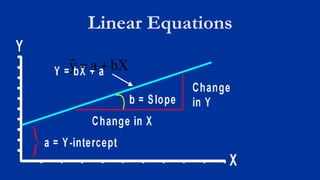
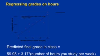
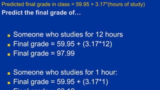
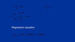
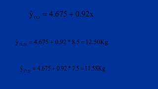
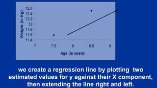
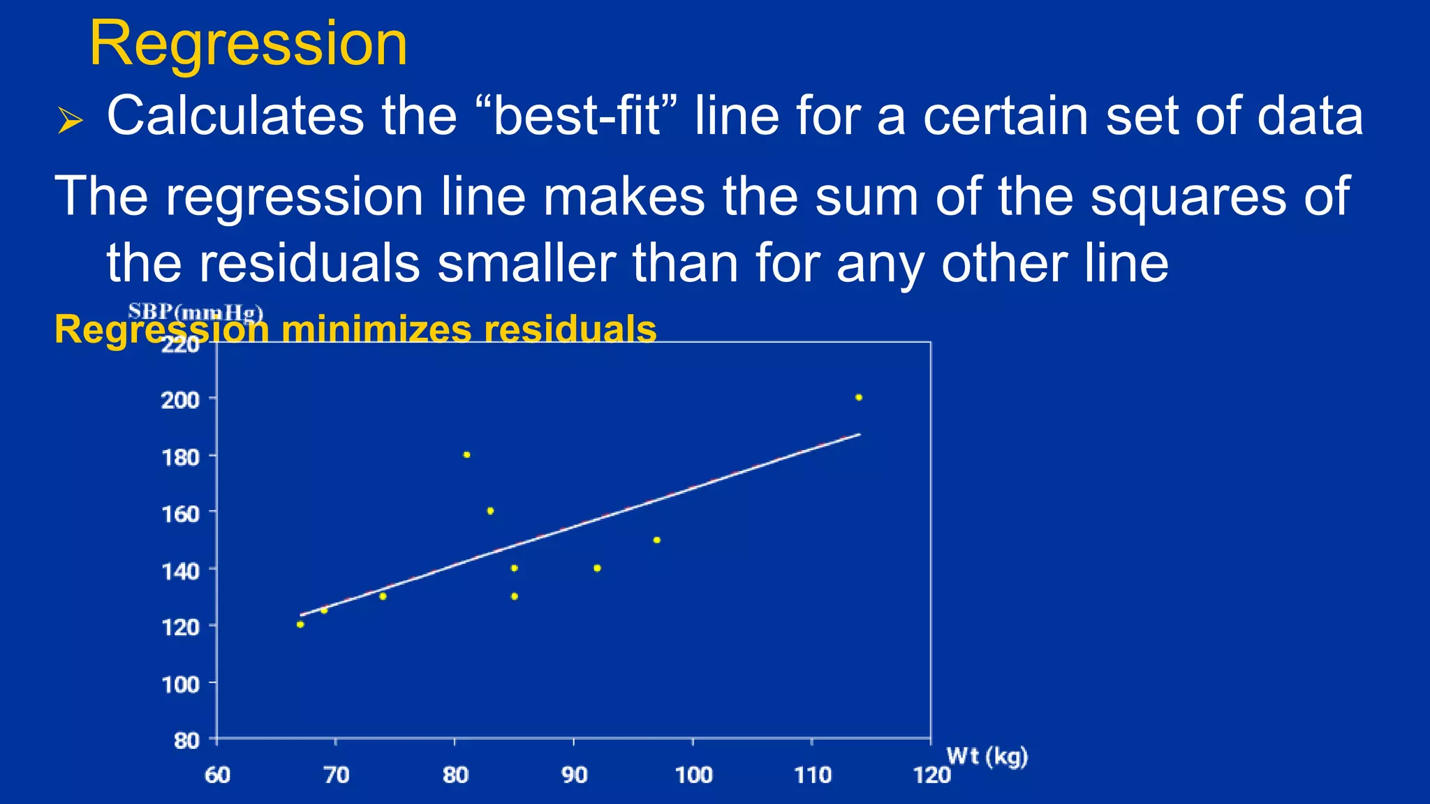
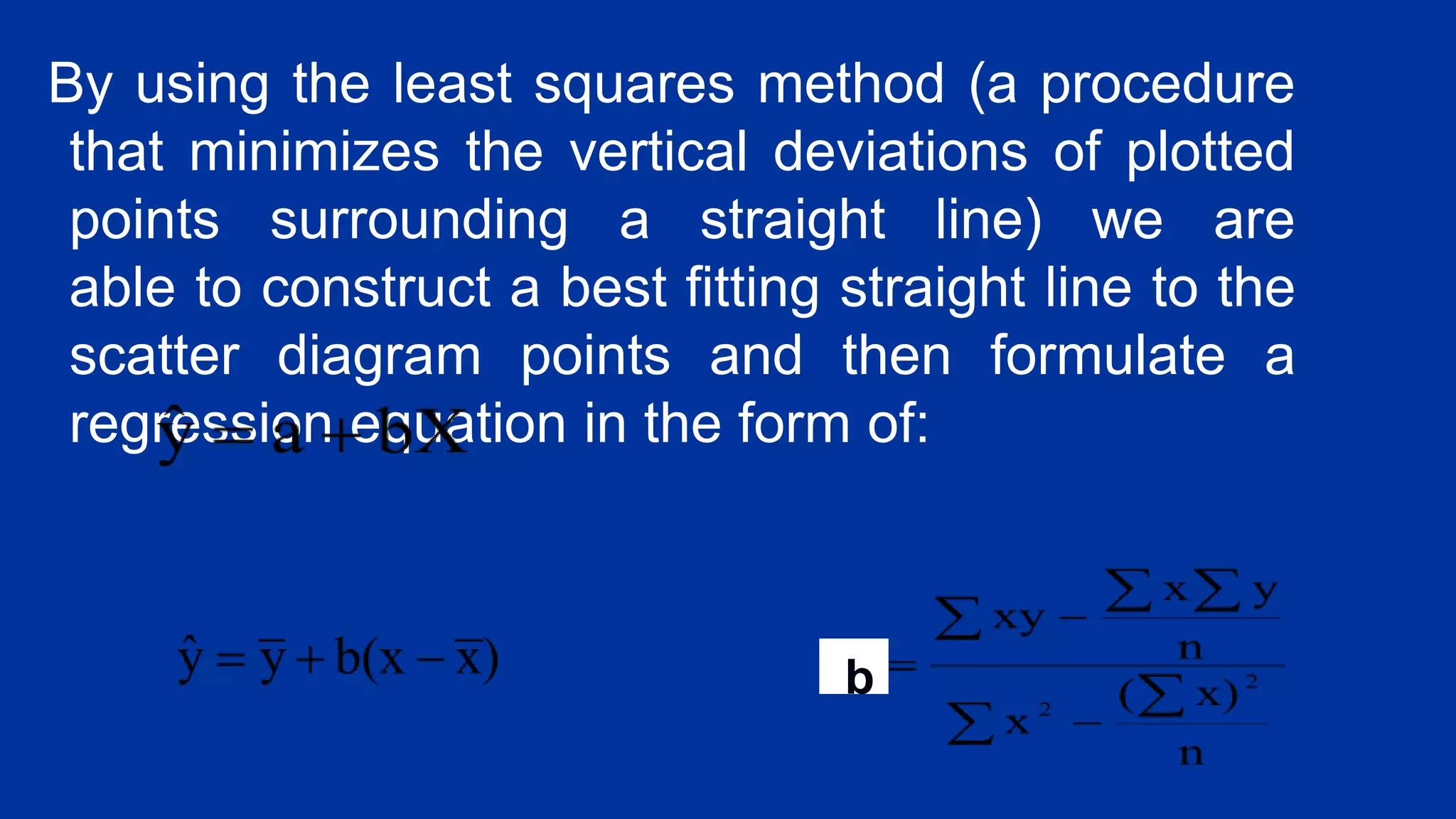
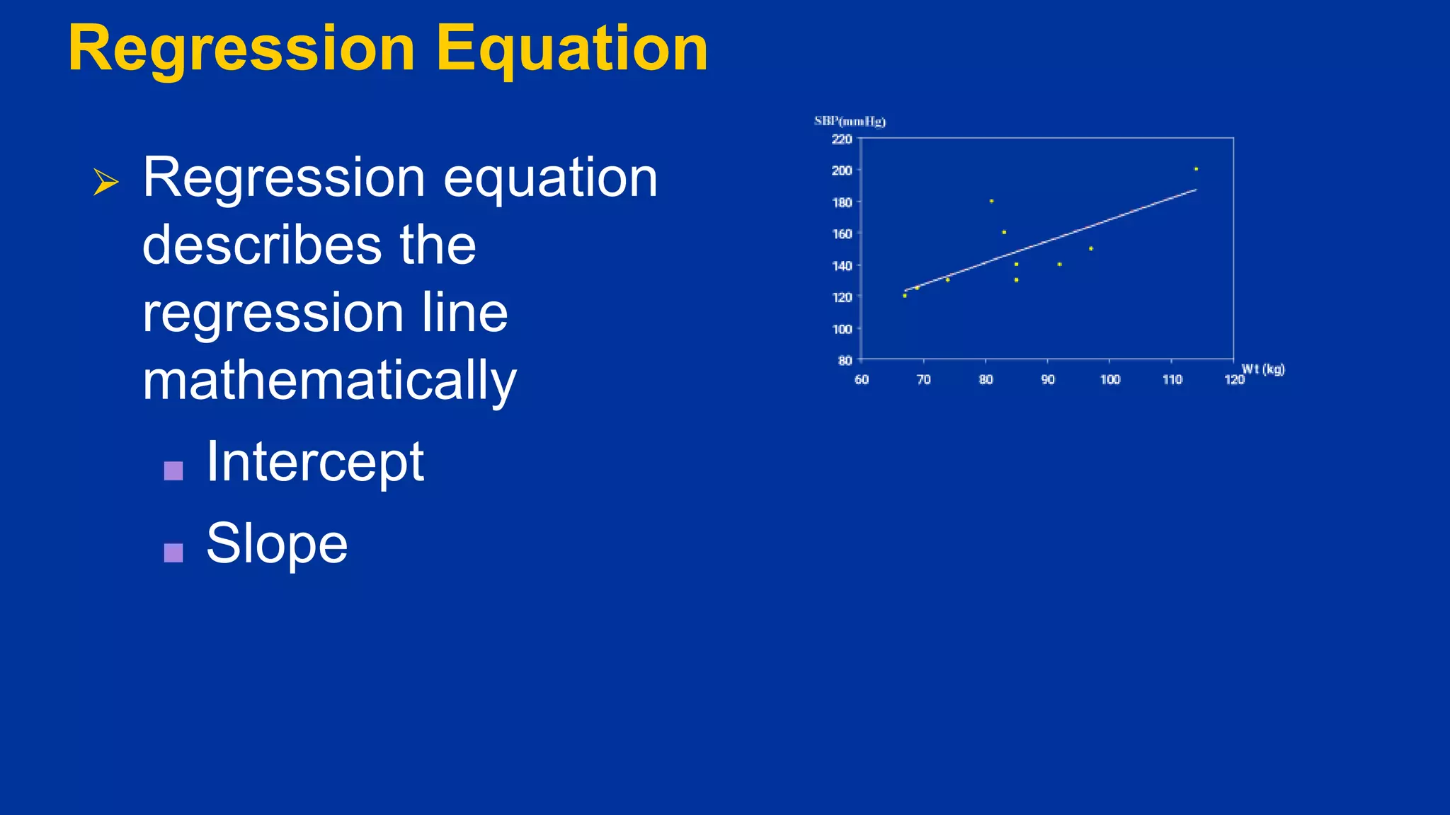
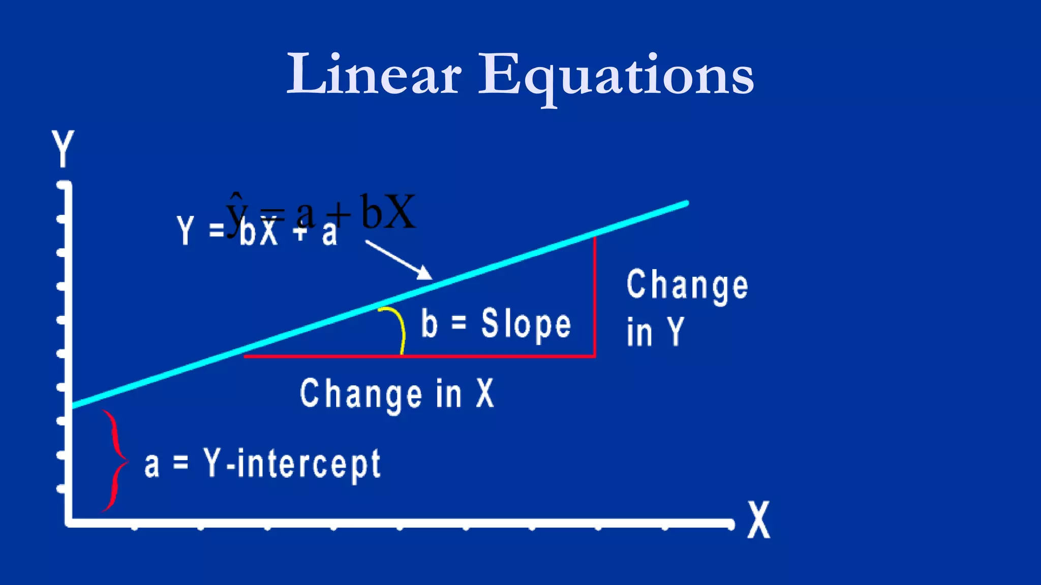
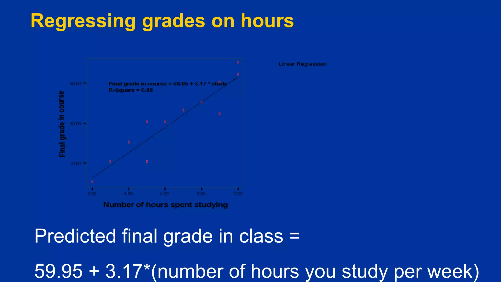
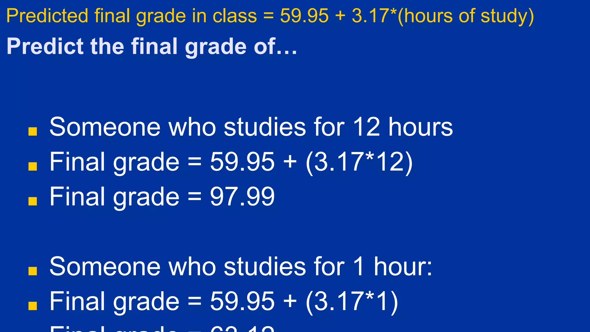
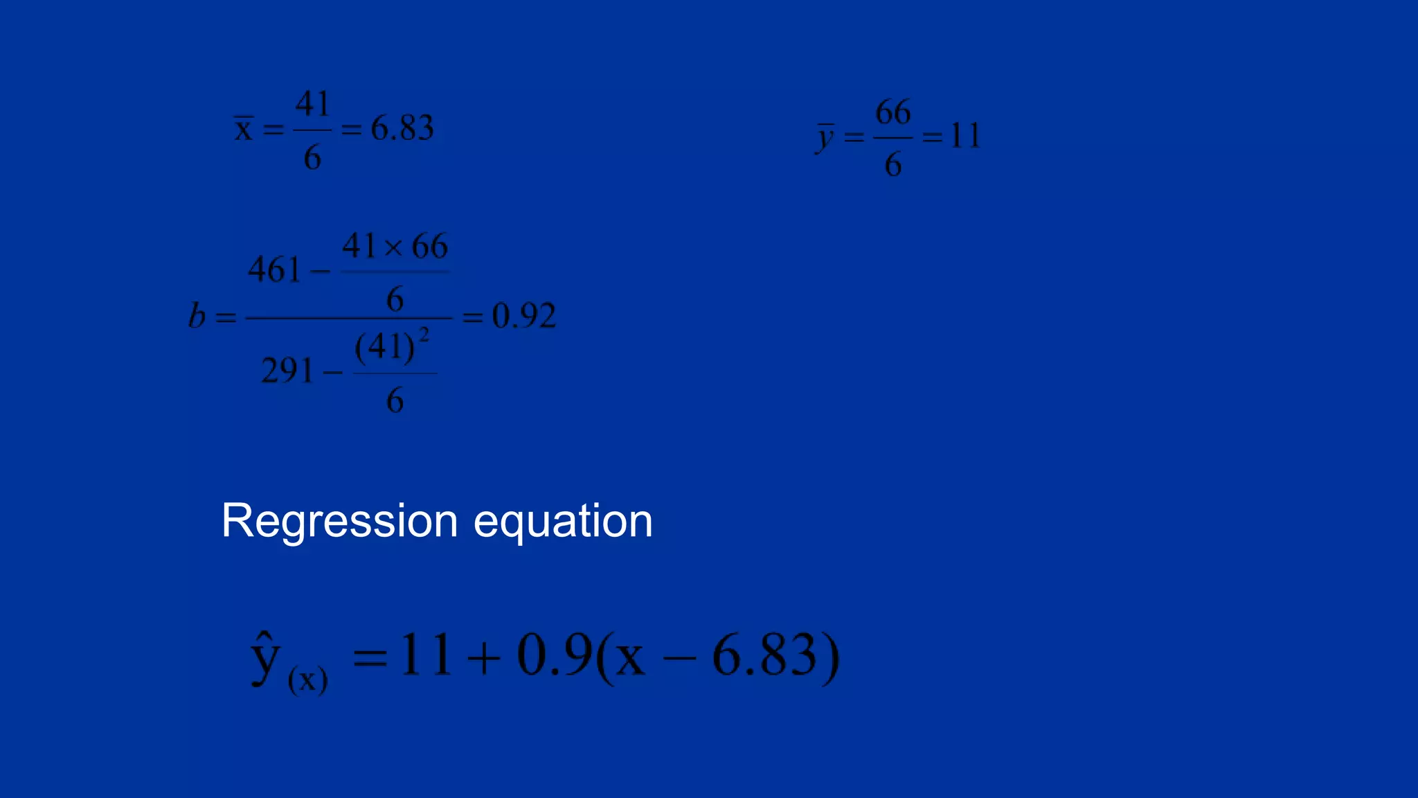
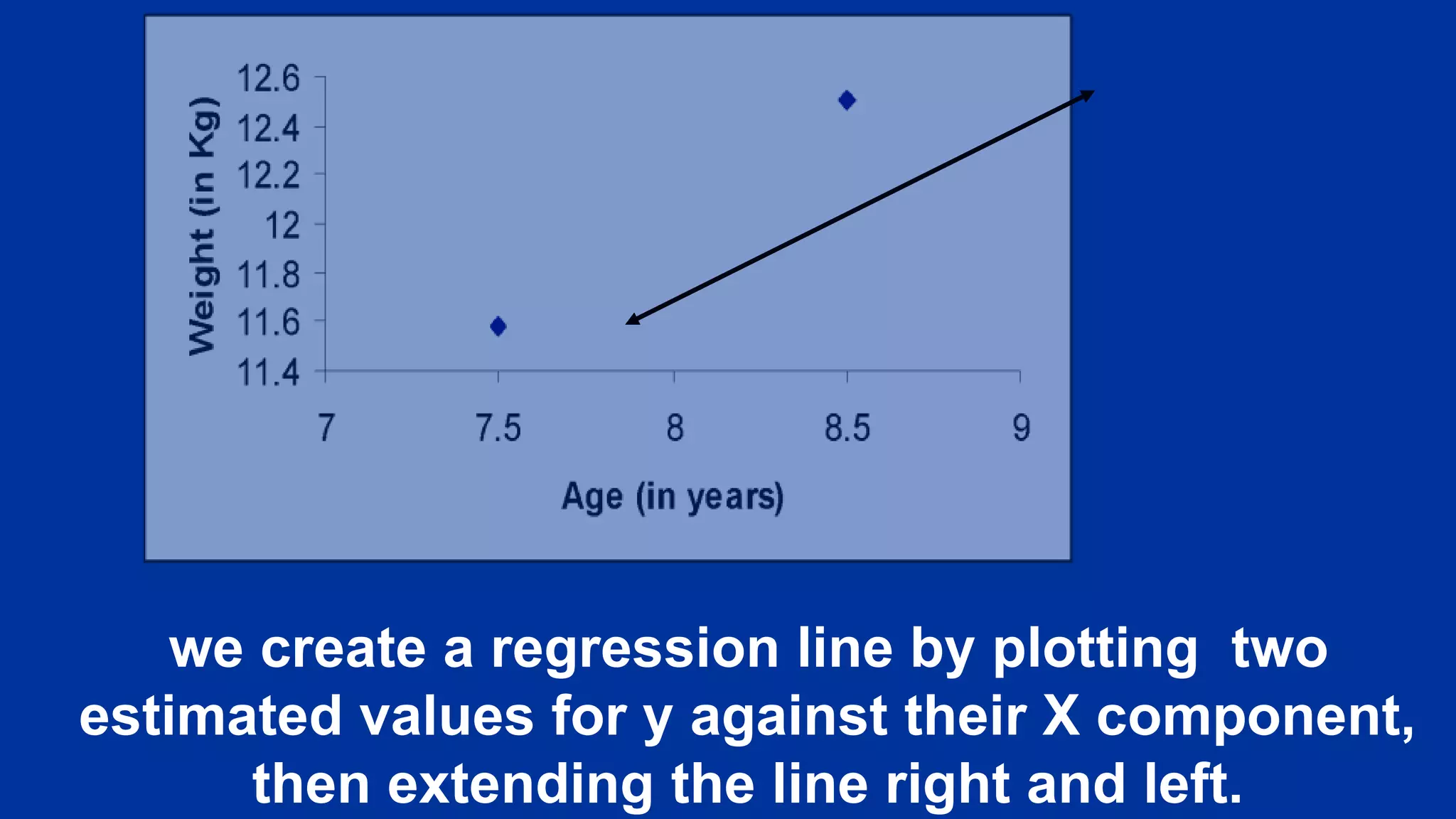
Understanding regression for predicting Y from X, distinguishing between correlation and regression, and creating regression equations with examples.
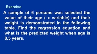
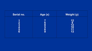
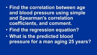
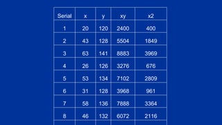
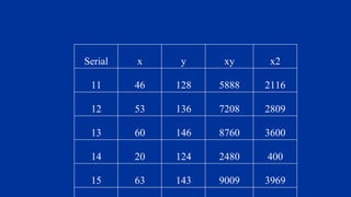
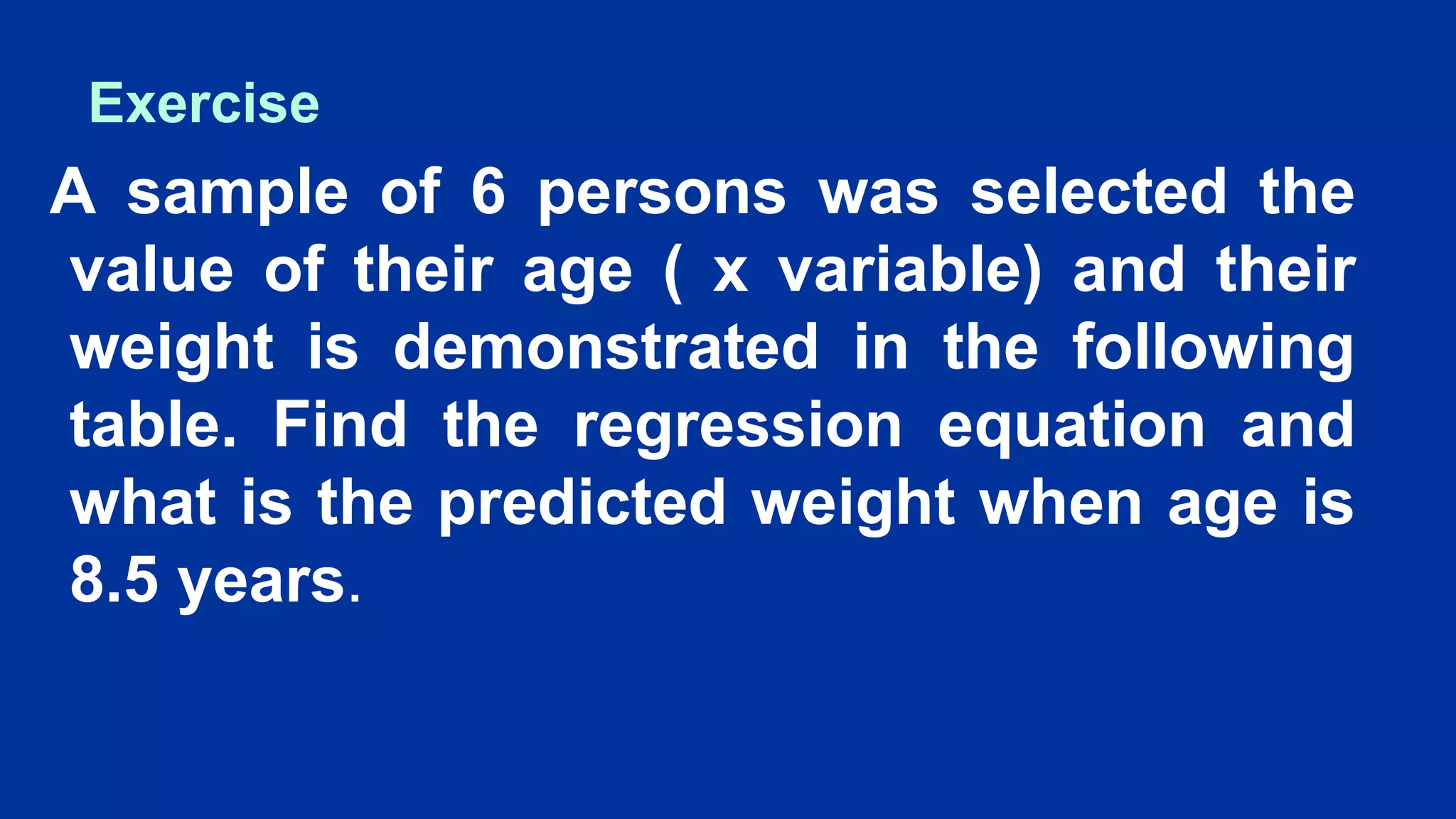
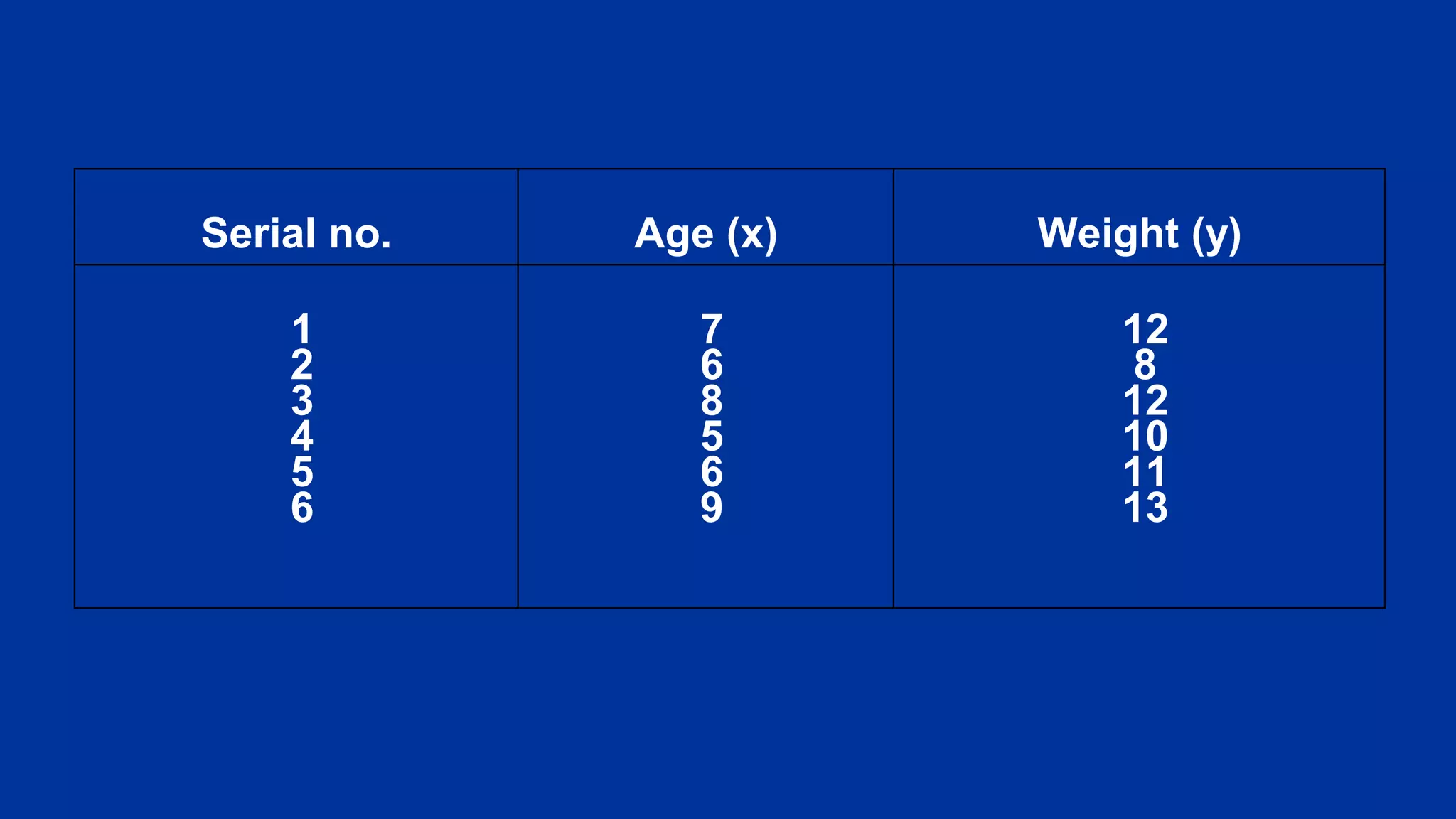
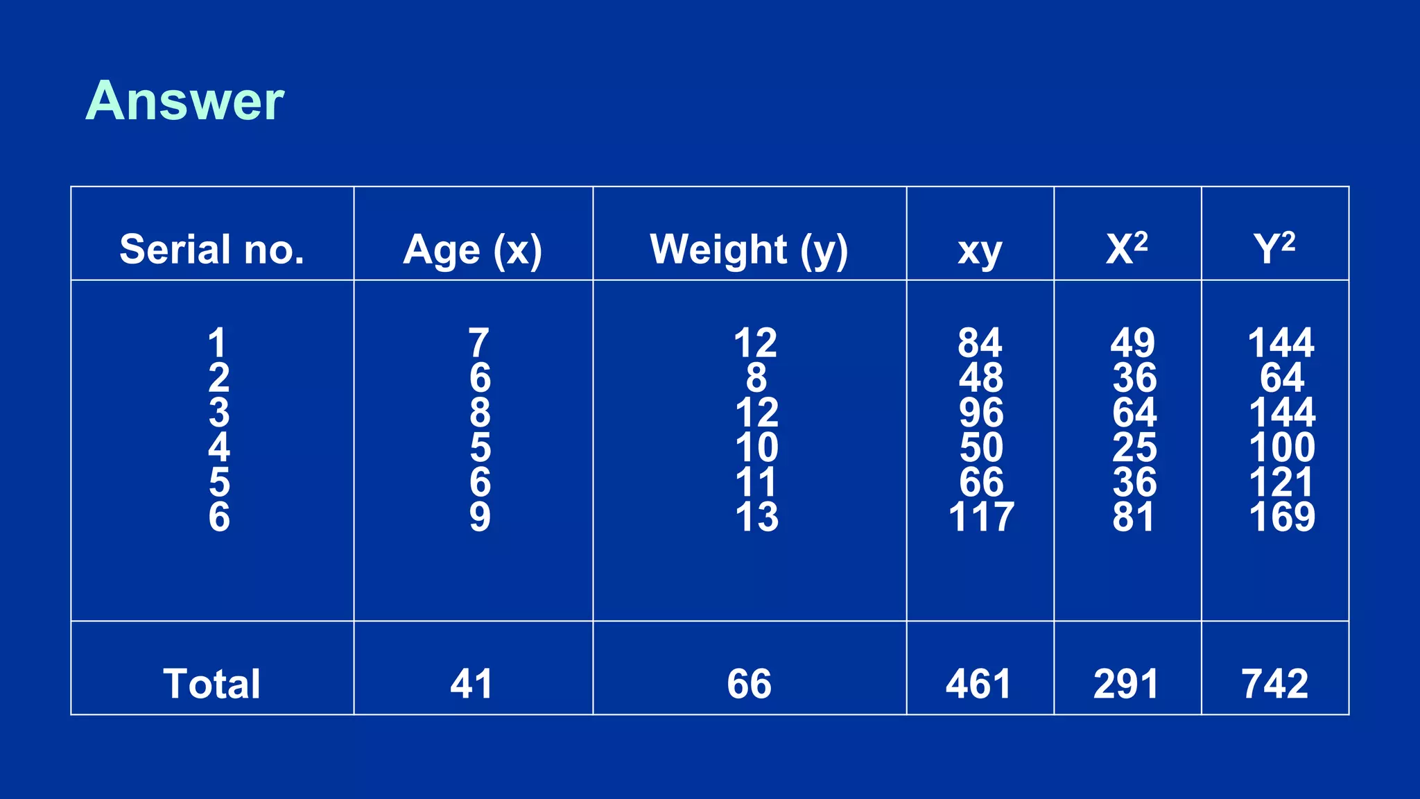
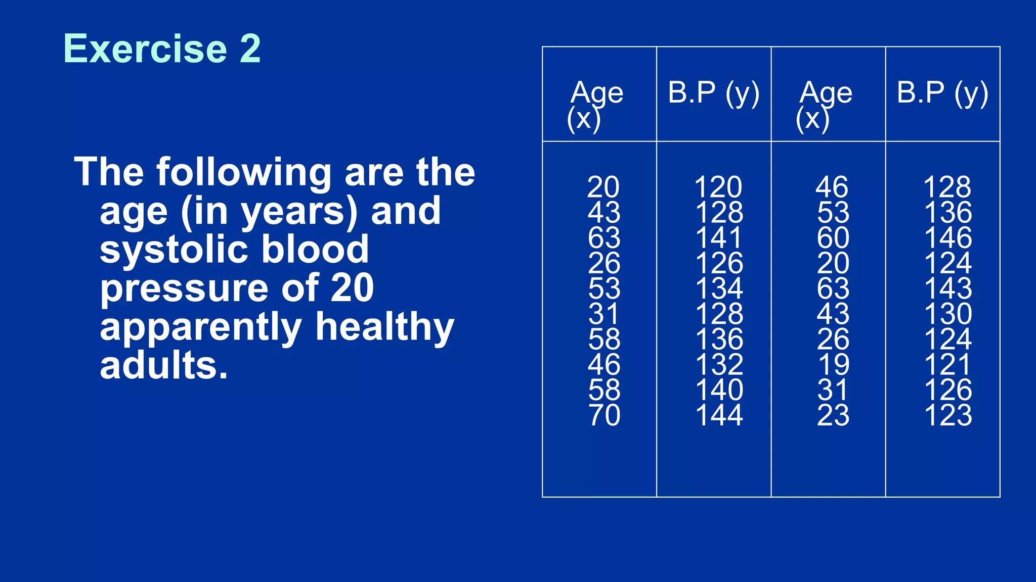
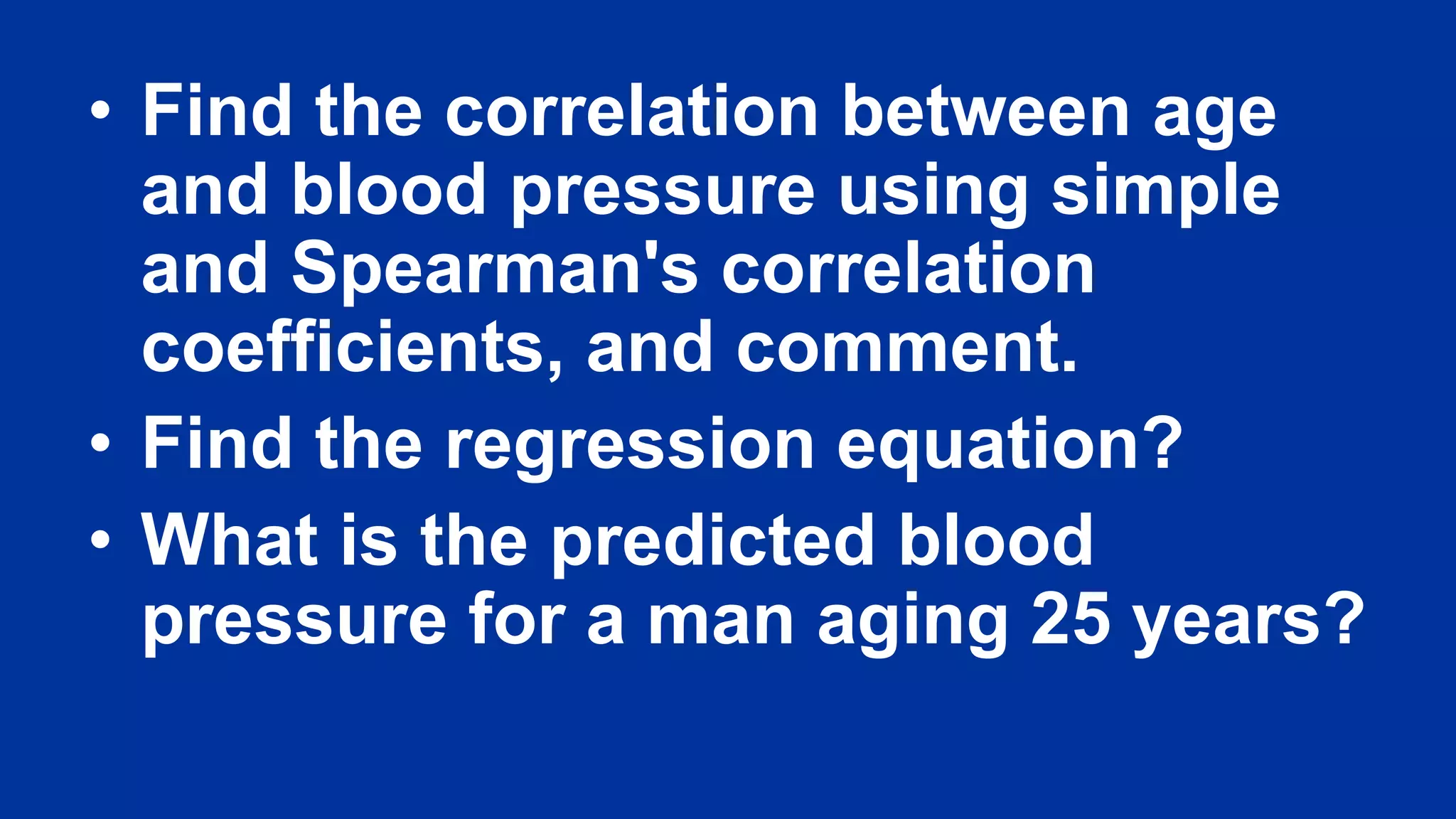
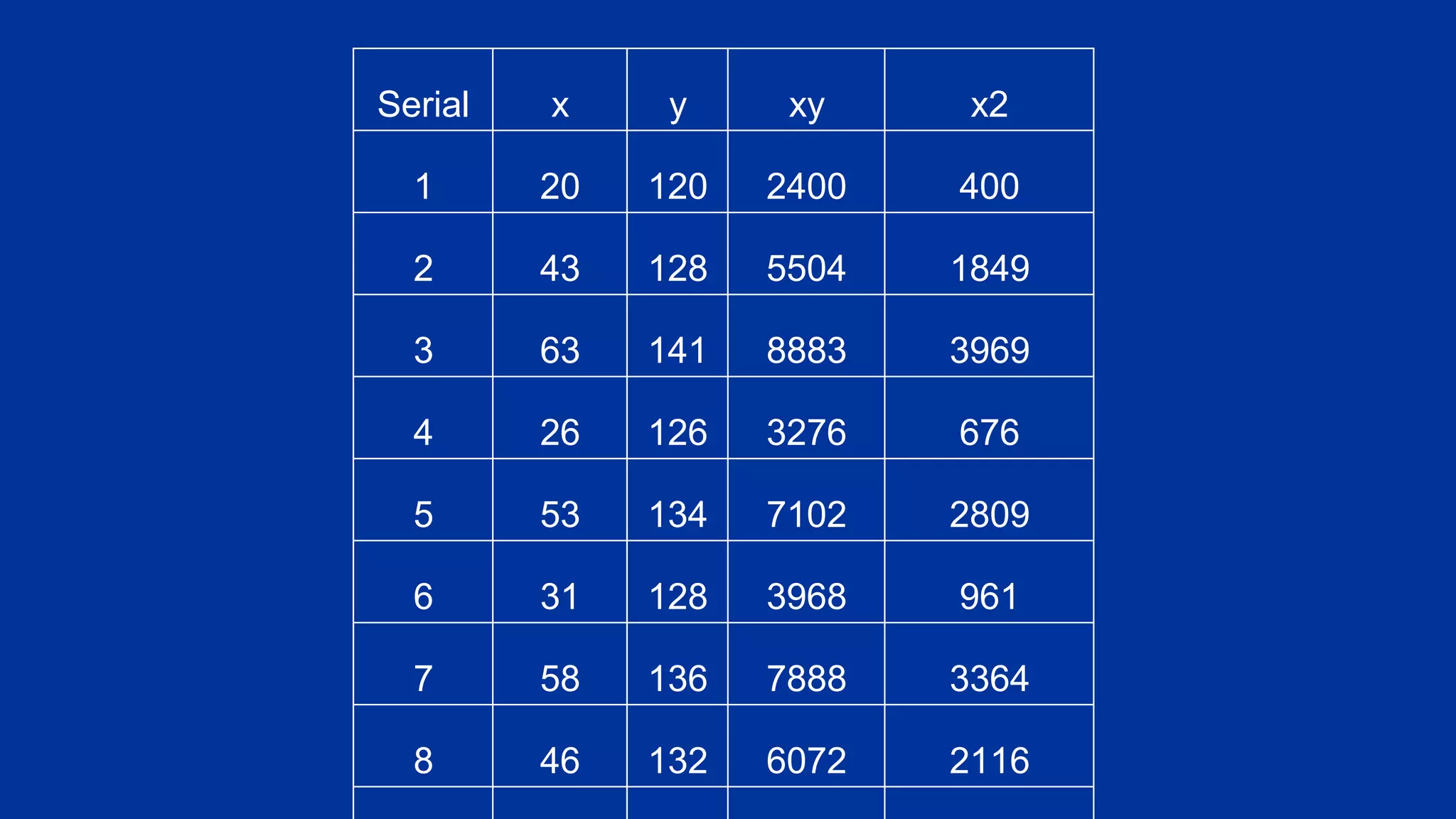
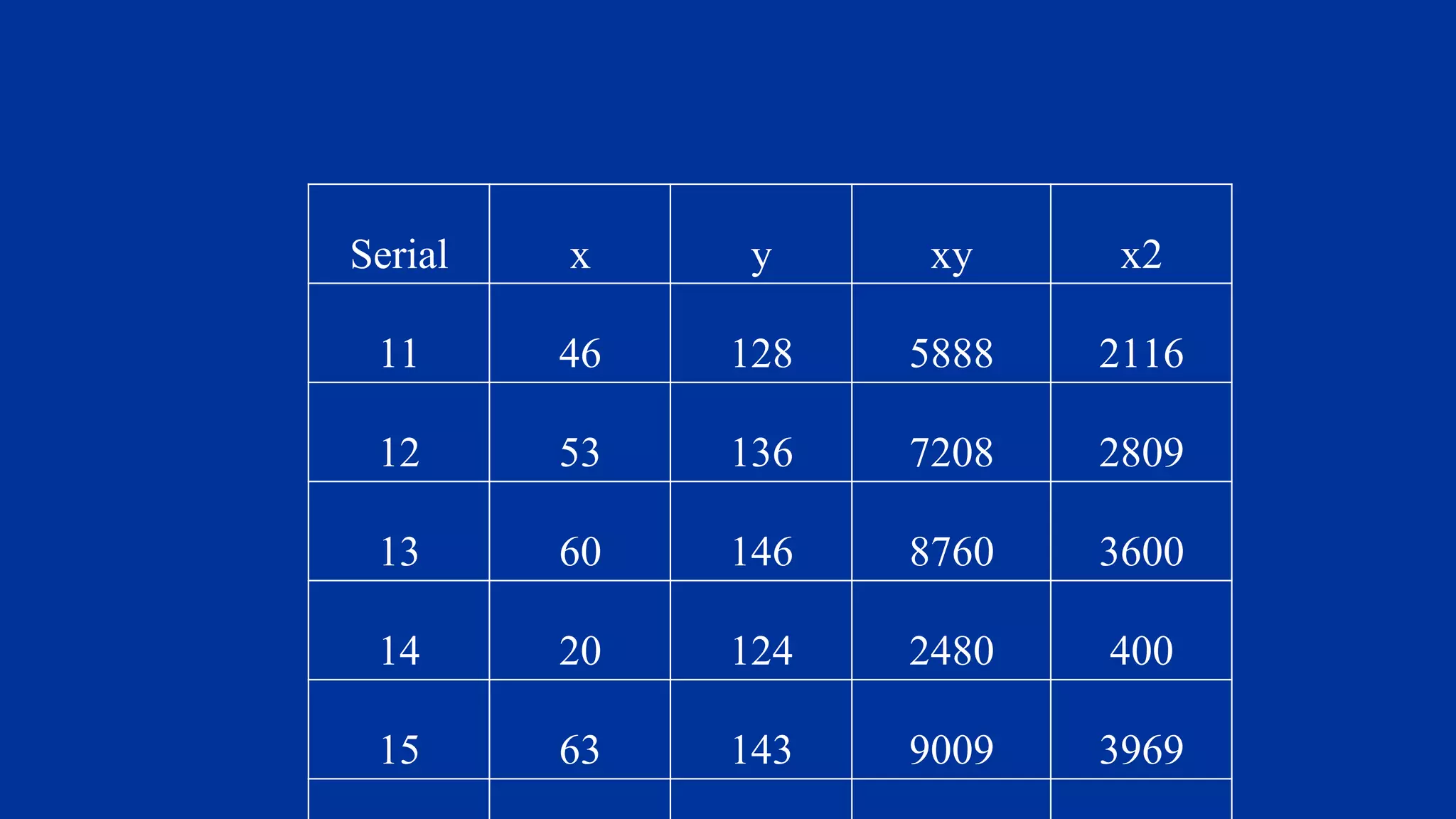
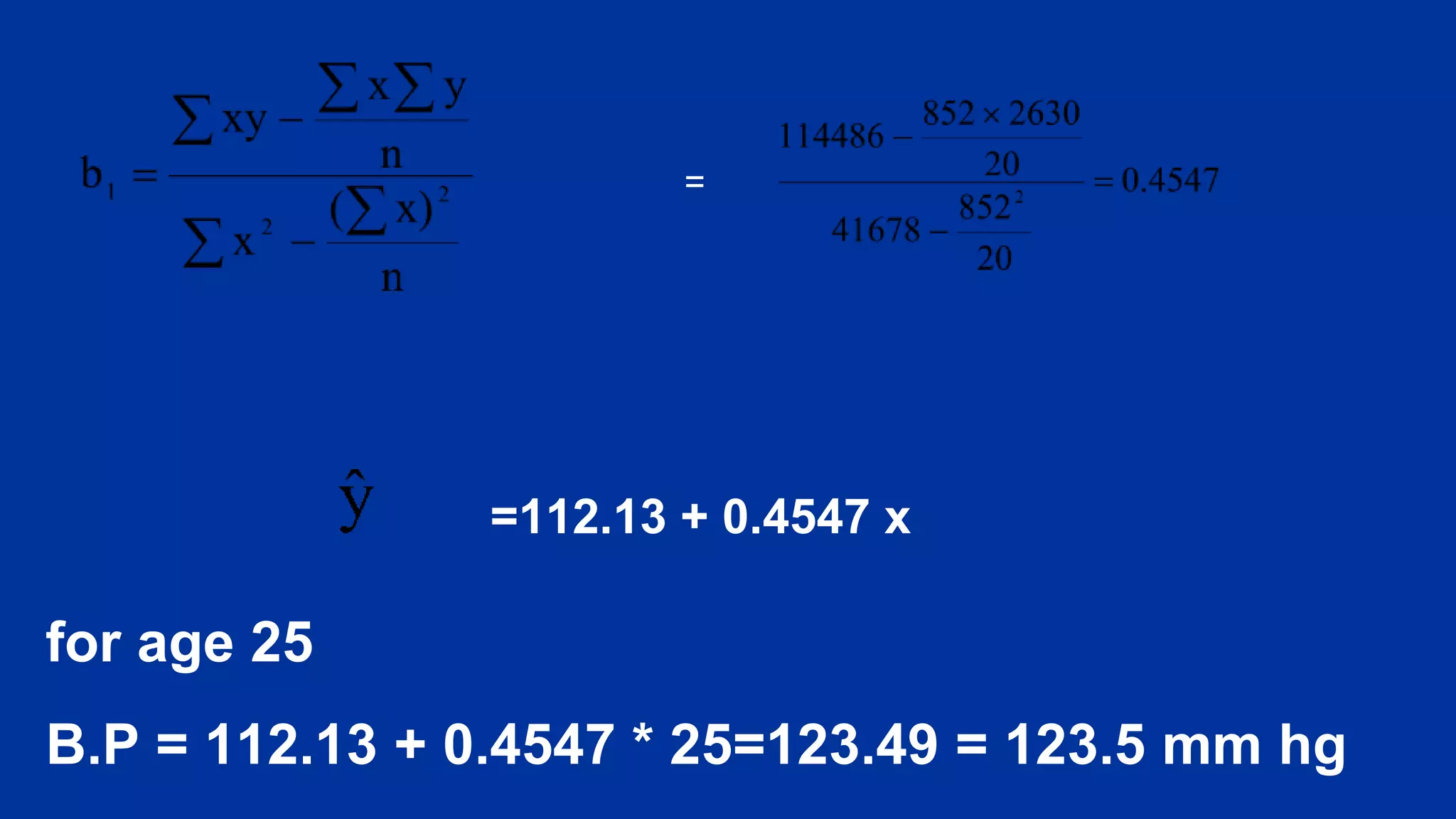
Exercises on finding regression equations and predicting values based on provided data sets for age and blood pressure.
Introduction to multiple regression analysis as an extension of simple regression, handling multiple independent variables.


