Reuqired ppt for machine learning algirthms and part
1.
Quick Insights aboutMachine learning, Neural
Network Algorithms, & AR Model
Siddhesh Mhatre
2.
Review Papers
Predictive analysis using machine learning: Review of trends and methods
Machine learning and deep learning based predictive quality in manufacturing: a systematic review
Healthcare predictive analytics using machine learning and deep learning techniques: a survey
3.
What isMachine learning?
It is a subset of Artificial Intelligence.
The ability of Machines to solve any kind of problem without being explicitly programmed.
Types of Machine learning: -
Supervised learning
Unsupervised learning
Semi-supervised learning
Reinforcement learning
4.
Supervised learning:-
Supervised learning is basically that kind of learning which we can used for labelled data or previously
available data. (i.e. Historical data)
And, It is further divided into two classes:-
1. Classification (Finds the relation between discrete input & output)
2. Regression (Finds the relation between two or more independent variables)
5.
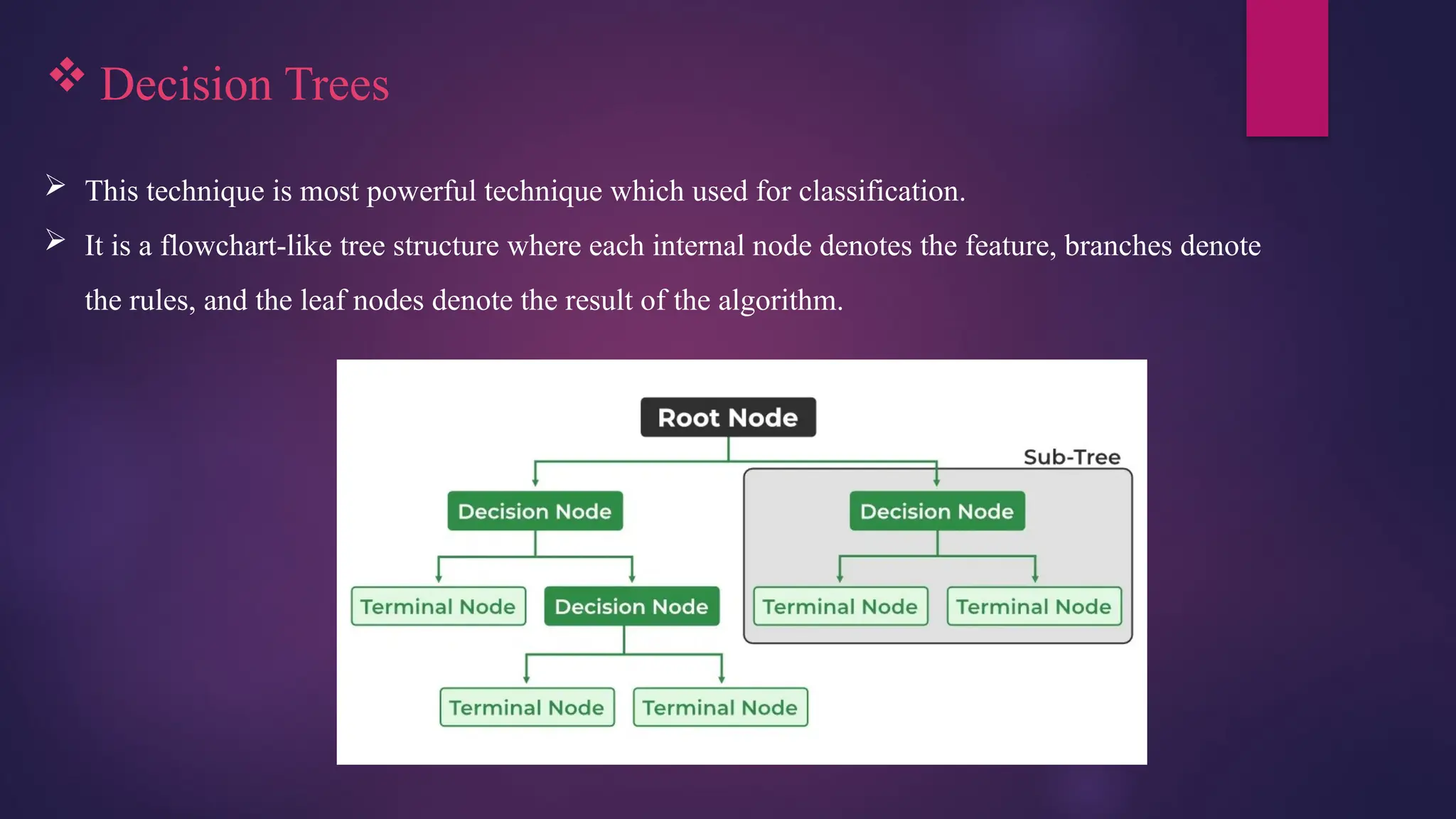
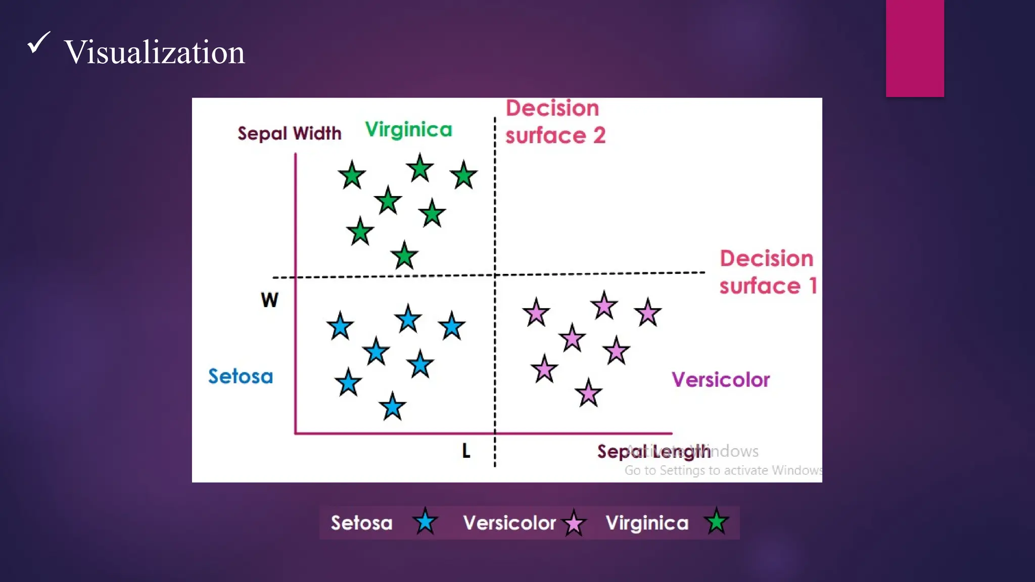
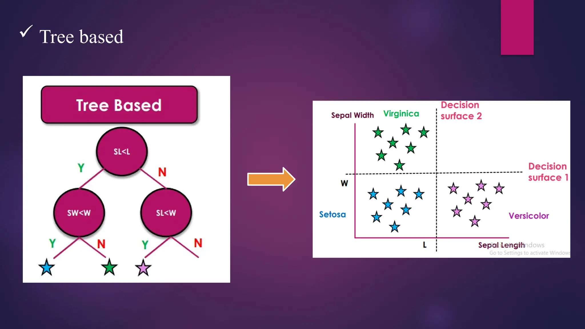
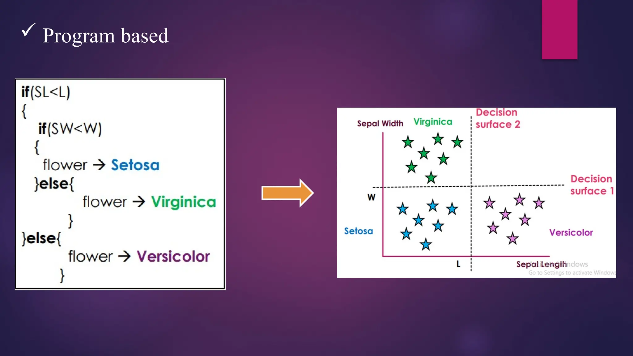
Decision Trees
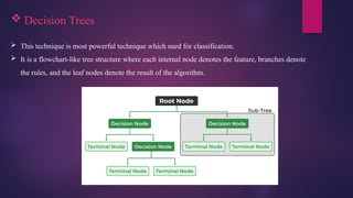
This technique is most powerful technique which used for classification.
It is a flowchart-like tree structure where each internal node denotes the feature, branches denote
the rules, and the leaf nodes denote the result of the algorithm.
Preliminary Conceptsused in Decision Tree are : -
Entropy
Gini Impurity
Information Gain
12.
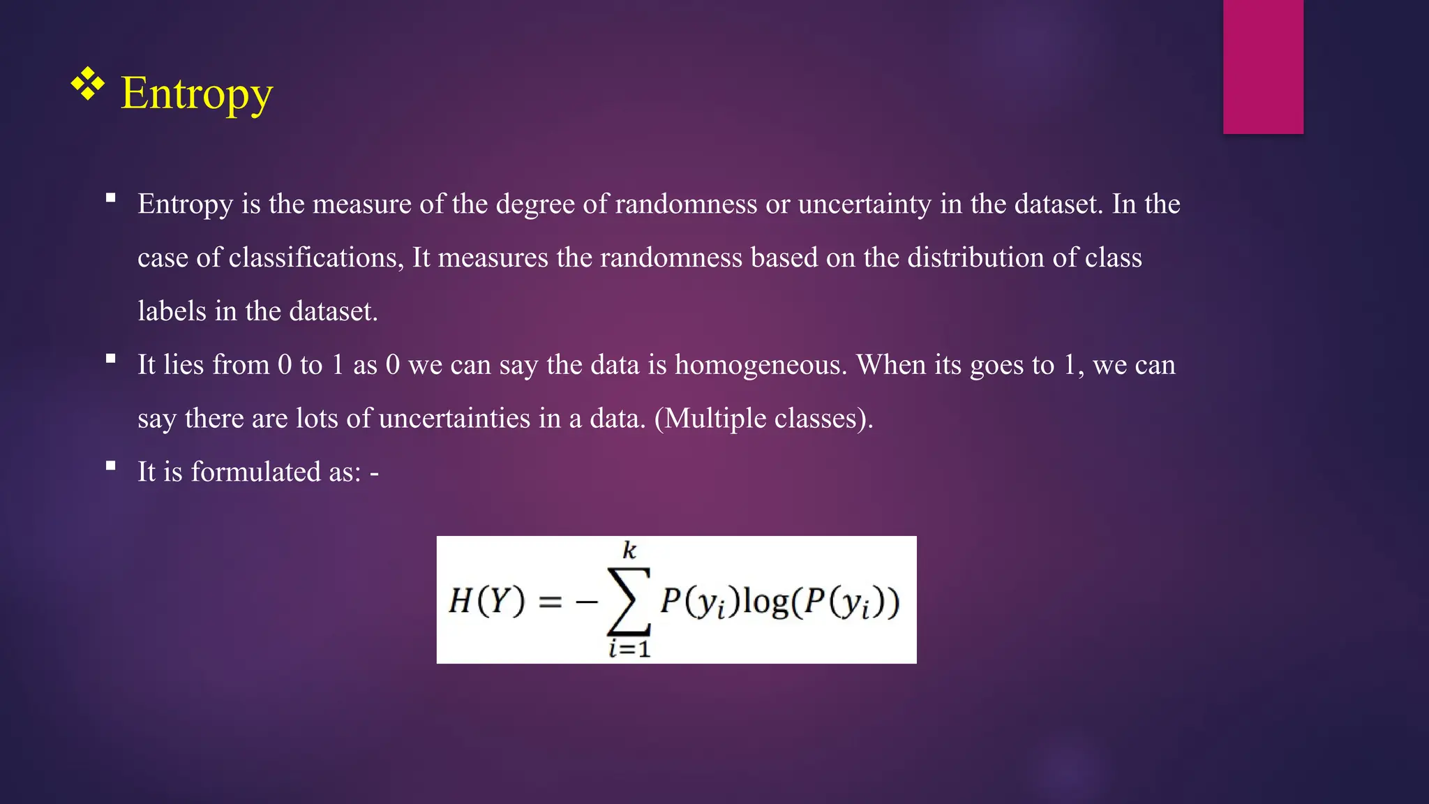
Entropy
Entropyis the measure of the degree of randomness or uncertainty in the dataset. In the
case of classifications, It measures the randomness based on the distribution of class
labels in the dataset.
It lies from 0 to 1 as 0 we can say the data is homogeneous. When its goes to 1, we can
say there are lots of uncertainties in a data. (Multiple classes).
It is formulated as: -
13.
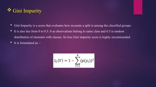
Gini Impurity
Gini Impurity is a score that evaluates how accurate a split is among the classified groups.
It is also lies from 0 to 0.5. 0 as observations belong to same class and 0.5 is random
distribution of elements with classes. So less Gini impurity score is highly recommended.
It is formulated as: -
14.
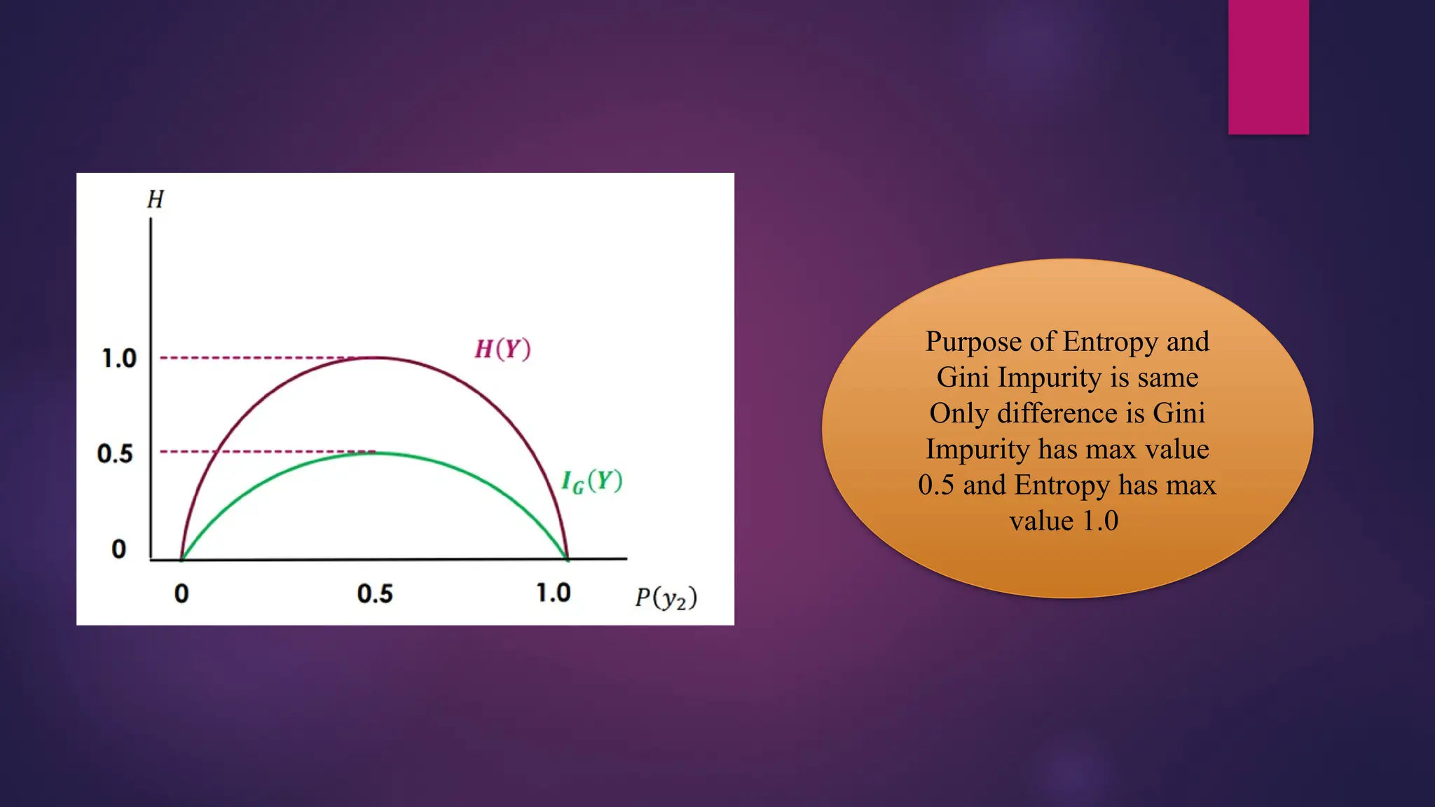
Purpose of Entropyand
Gini Impurity is same
Only difference is Gini
Impurity has max value
0.5 and Entropy has max
value 1.0
15.
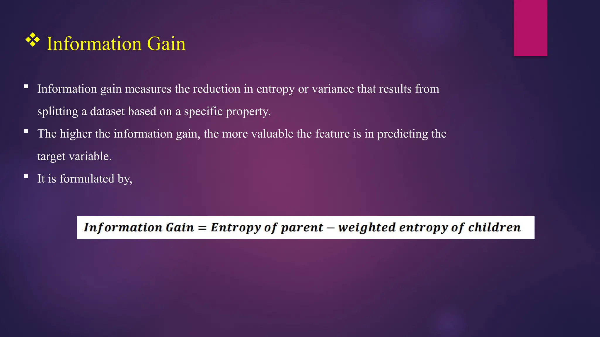
Information Gain
Information gain measures the reduction in entropy or variance that results from
splitting a dataset based on a specific property.
The higher the information gain, the more valuable the feature is in predicting the
target variable.
It is formulated by,
16.
Hyperparameters
Hyperparameters comingunder Decision tree are: -
Pure node
Maximum number of leaf nodes
Minimum Information gain
Maximum Depth
Minimum samples at leaf node
Minimum impurity to split
17.
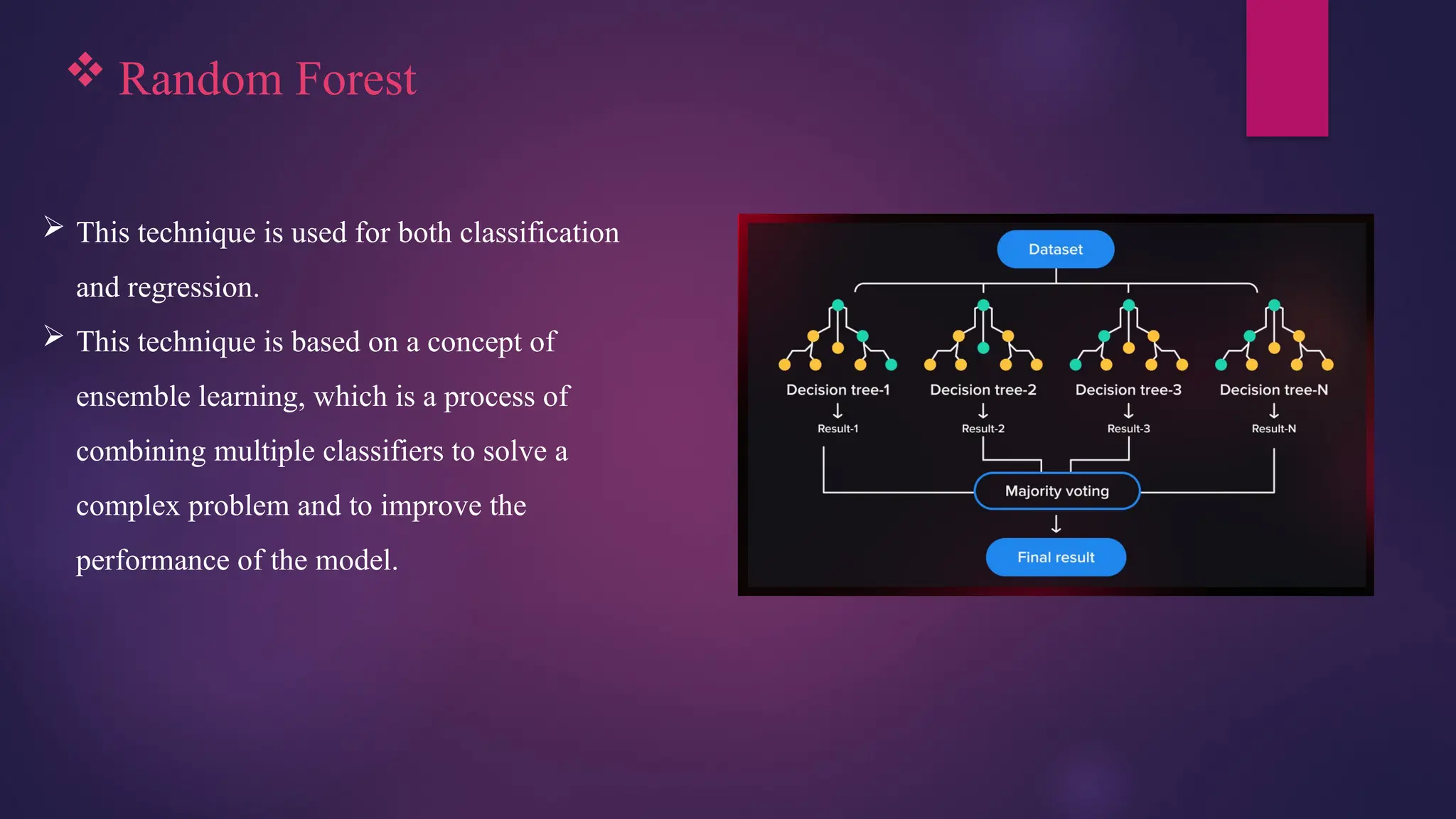
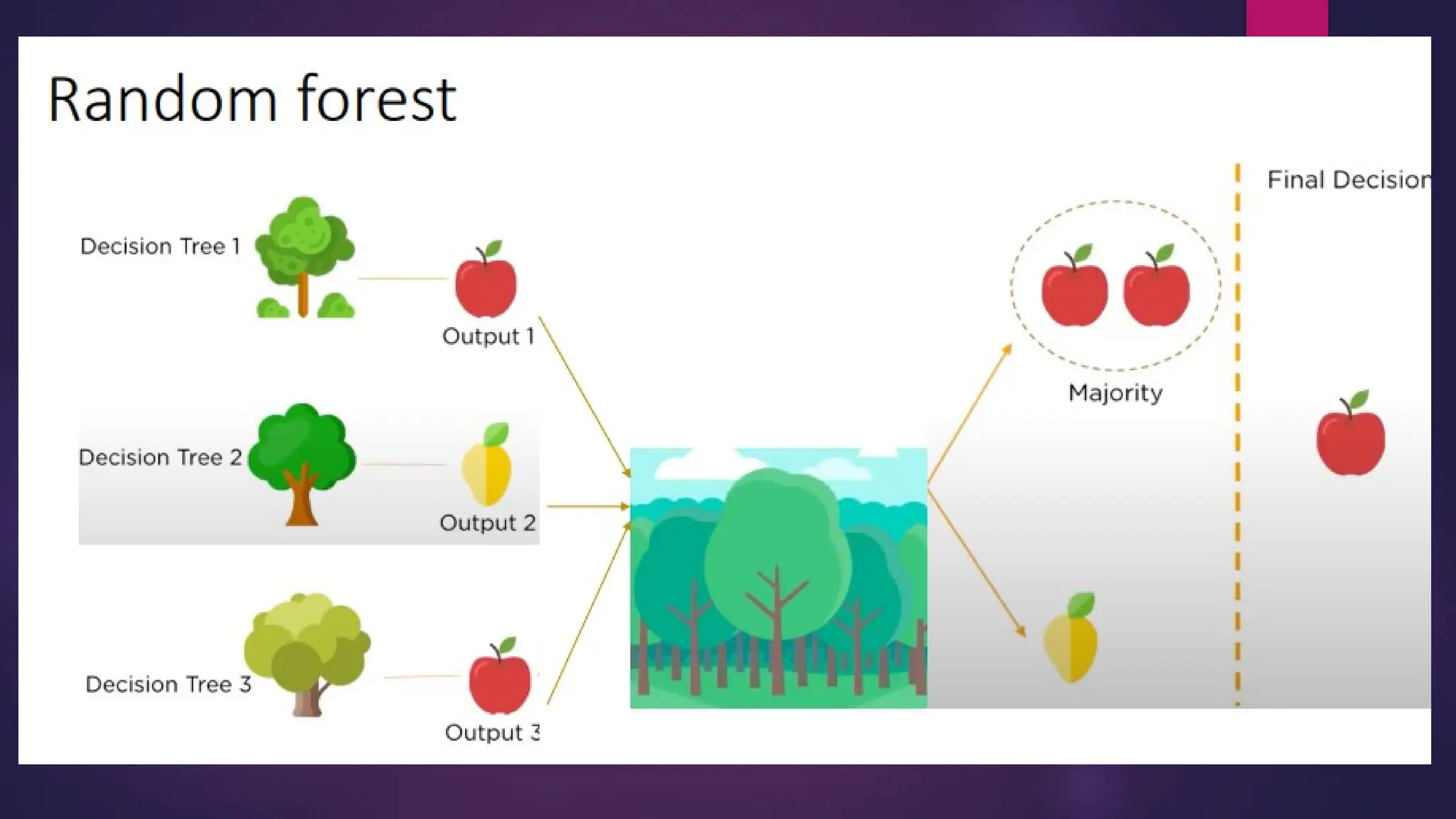
Random Forest
This technique is used for both classification
and regression.
This technique is based on a concept of
ensemble learning, which is a process of
combining multiple classifiers to solve a
complex problem and to improve the
performance of the model.
19.
Ensemble models
•Ensemble – Group of things Combine different ML models to create a more powerful
model.
Following Ensemble models are: -
1. Bagging
2. Boosting
3. Stacking
4. Cascading
20.
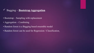
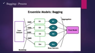
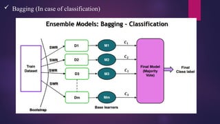
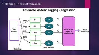
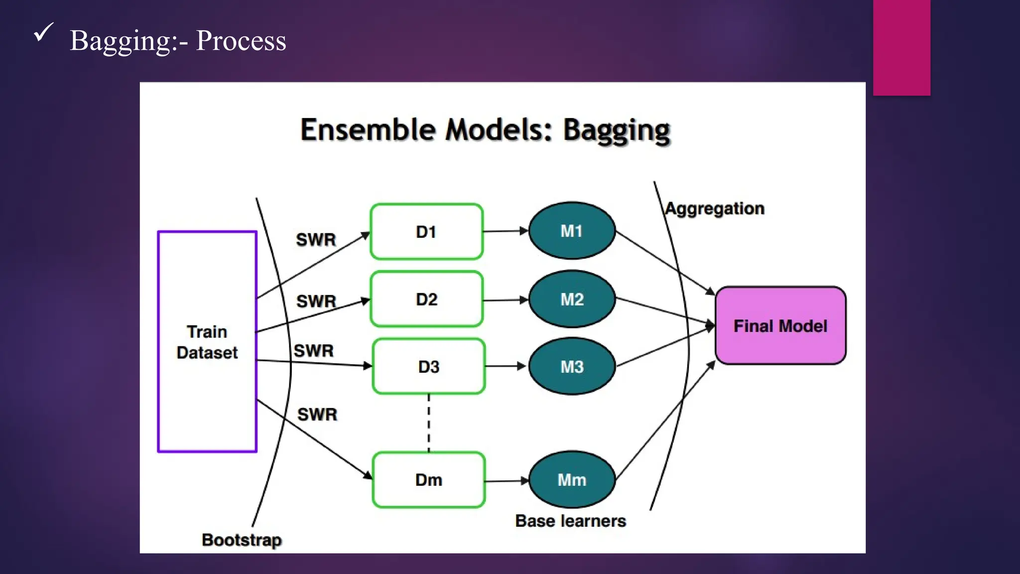
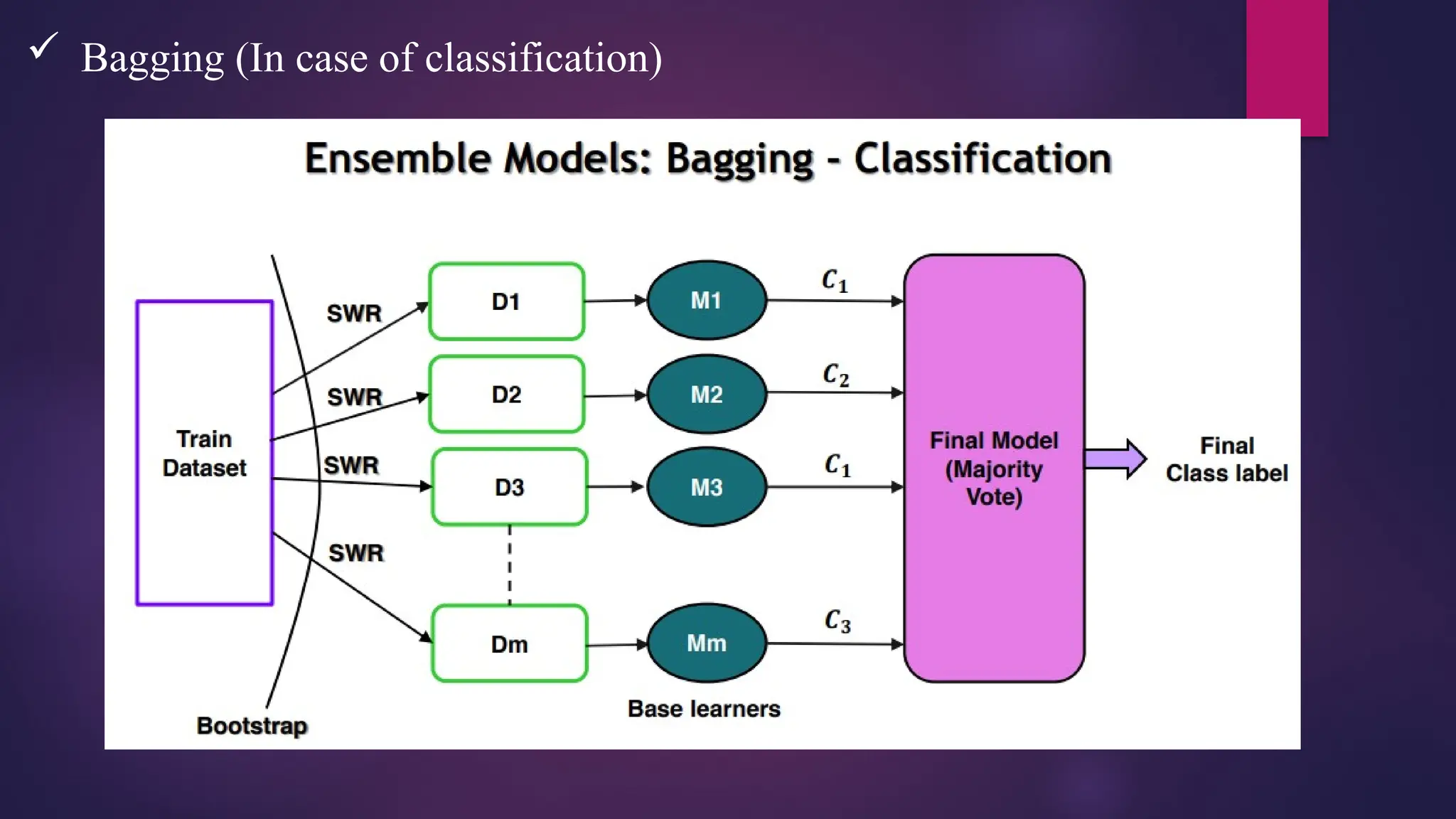
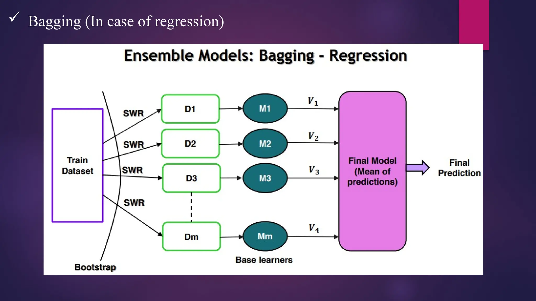
Bagging –Bootstrap Aggregation
• Bootstrap – Sampling with replacement
• Aggregation – Combining
• Random forest is a Bagging based ensemble model
• Random forest can be used for Regression / Classification
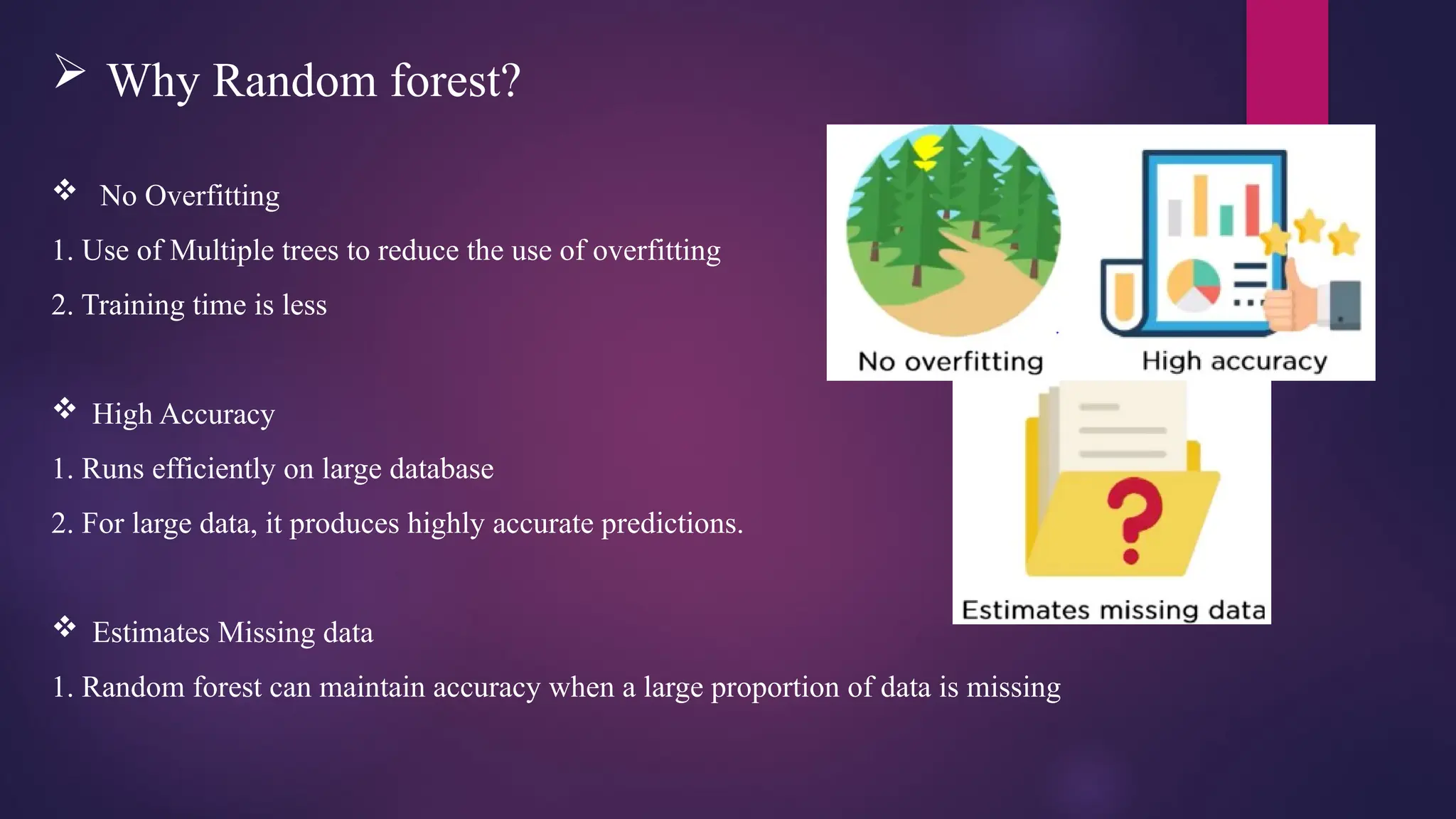
Why Randomforest?
No Overfitting
1. Use of Multiple trees to reduce the use of overfitting
2. Training time is less
High Accuracy
1. Runs efficiently on large database
2. For large data, it produces highly accurate predictions.
Estimates Missing data
1. Random forest can maintain accuracy when a large proportion of data is missing
26.
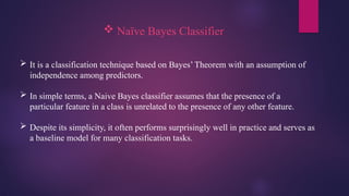
Naïve BayesClassifier
It is a classification technique based on Bayes’ Theorem with an assumption of
independence among predictors.
In simple terms, a Naive Bayes classifier assumes that the presence of a
particular feature in a class is unrelated to the presence of any other feature.
Despite its simplicity, it often performs surprisingly well in practice and serves as
a baseline model for many classification tasks.
27.
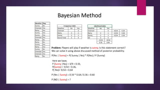
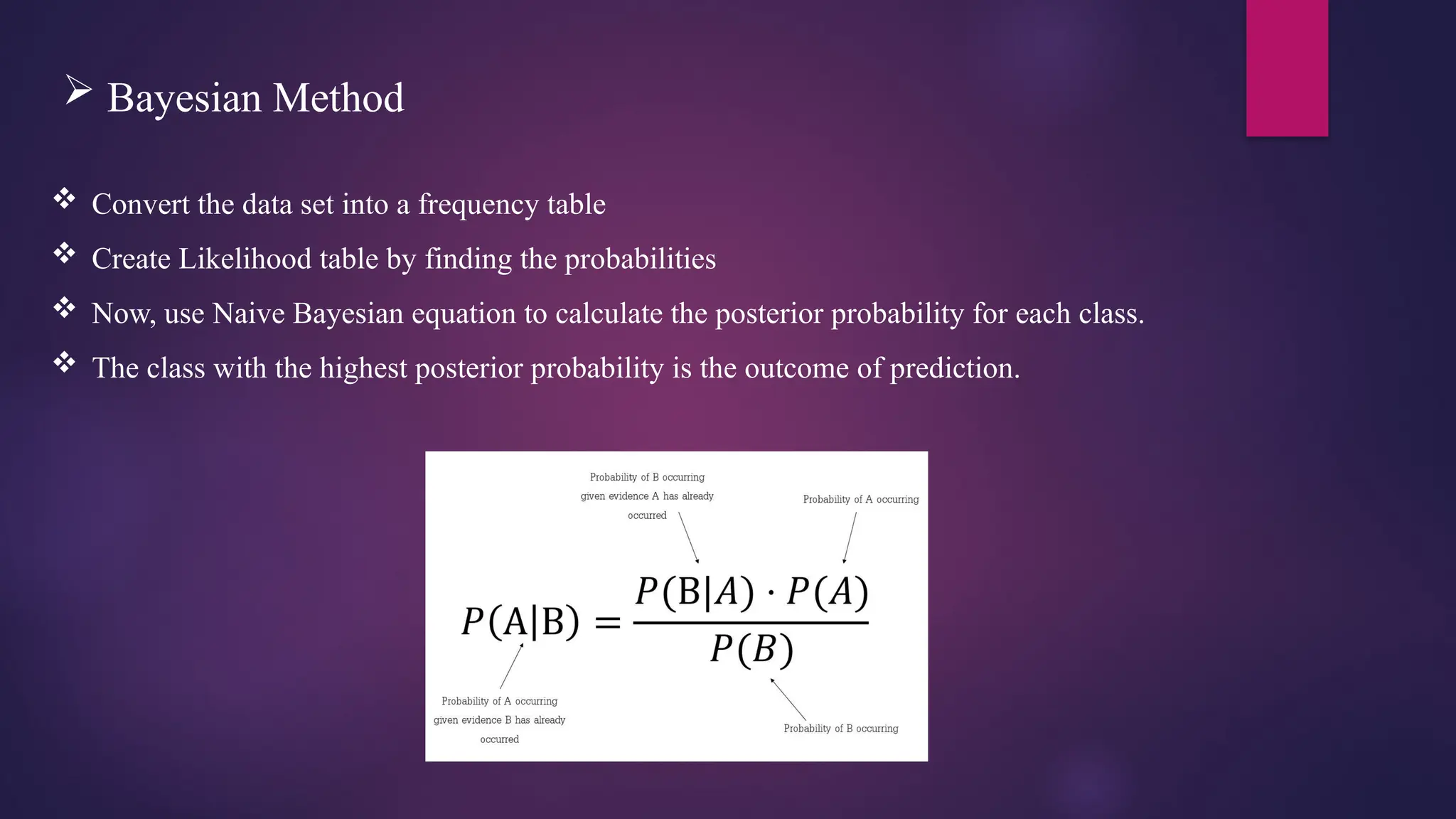
Bayesian Method
Convert the data set into a frequency table
Create Likelihood table by finding the probabilities
Now, use Naive Bayesian equation to calculate the posterior probability for each class.
The class with the highest posterior probability is the outcome of prediction.
29.
Types ofNaive Bayes
1. Gaussian Naïve Bayes: -
• Variables are continuous in nature.
• It assumes that all the variables have a normal distribution
2. Multinominal Naïve Bayes: -
• The features represent the frequency.
• If you have a text document, and you extract all the unique words and create multiple features
where each feature represents the count of the word in the document.
3. Bernoulli Naïve Bayes: -
• This is used when features are binary.
30.
Pros:
It iseasy and fast to predict class of test data set. It also perform well in multi class
prediction.
When assumption of independence holds, a Naive Bayes classifier performs better
compared to other models like logistic regression and you need less training data.
It perform well in case of categorical input variables compared to numerical
variable(s).
31.
Cons:
If categorical variablehas a category (in test data set), which was not observed in training data set,
then model will assign a 0 (zero) probability and will be unable to make a prediction. This is often known
as “Zero Frequency”. To solve this, we can use the smoothing technique. One of the simplest smoothing
techniques is called Laplace estimation.
On the other side naive Bayes is also known as a bad estimator, so the probability outputs
from predict_proba are not to be taken too seriously.
Another limitation of Naive Bayes is the assumption of independent predictors. In real life, it is almost
impossible that we get a set of predictors which are completely independent.
32.
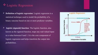
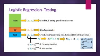
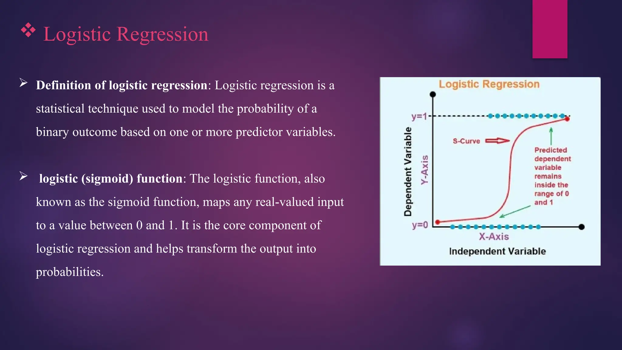
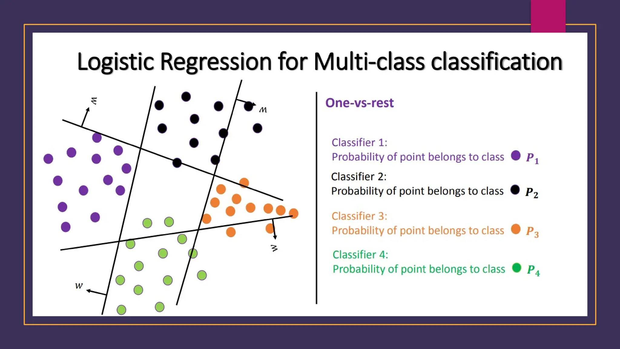
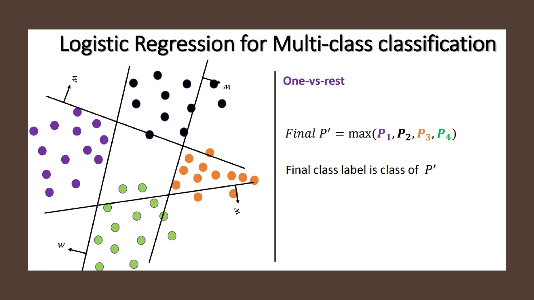
Logistic Regression
Definition of logistic regression: Logistic regression is a
statistical technique used to model the probability of a
binary outcome based on one or more predictor variables.
logistic (sigmoid) function: The logistic function, also
known as the sigmoid function, maps any real-valued input
to a value between 0 and 1. It is the core component of
logistic regression and helps transform the output into
probabilities.
33.
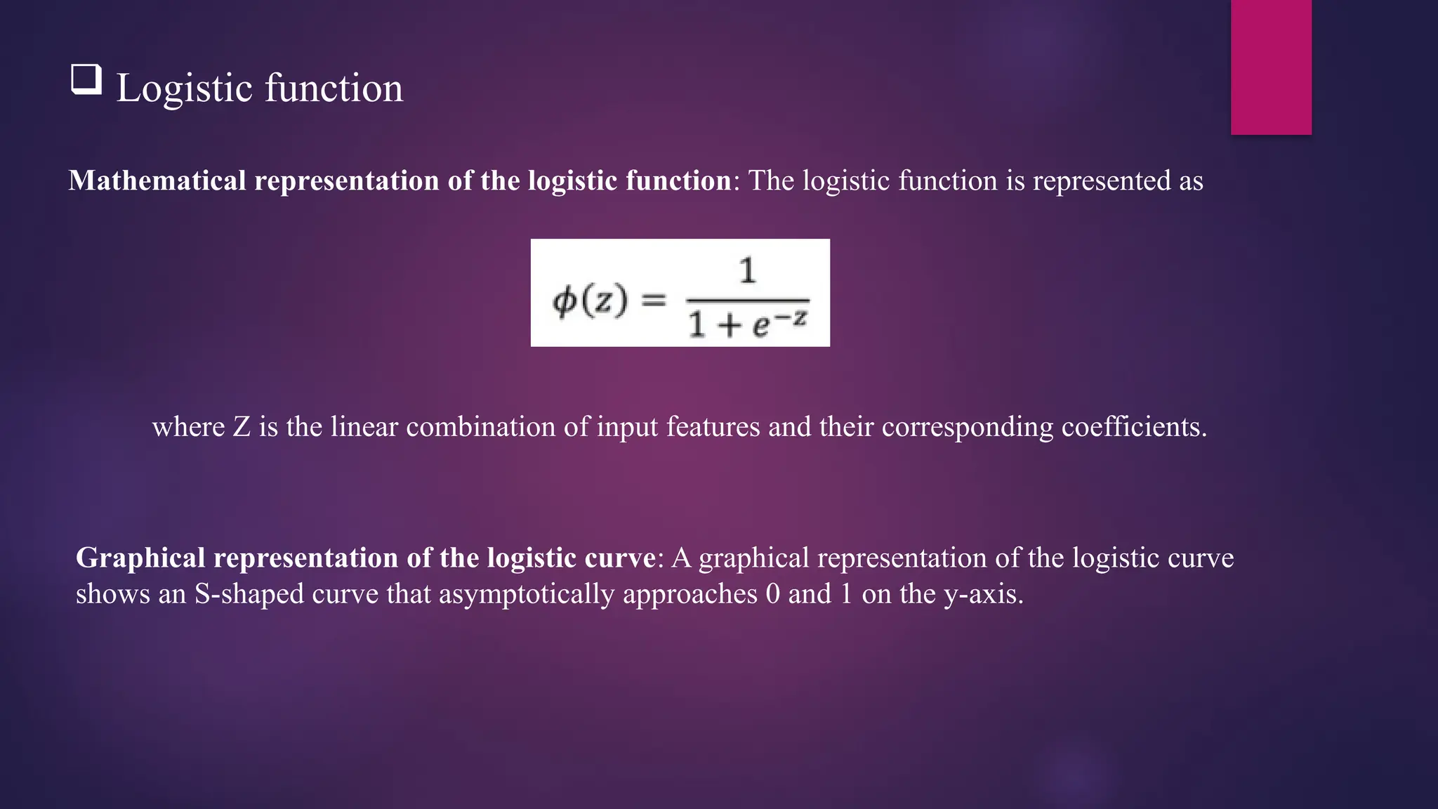
Logistic function
Mathematicalrepresentation of the logistic function: The logistic function is represented as
where Z is the linear combination of input features and their corresponding coefficients.
Graphical representation of the logistic curve: A graphical representation of the logistic curve
shows an S-shaped curve that asymptotically approaches 0 and 1 on the y-axis.
35.
Advantages andLimitations
Advantages of logistic regression: Logistic regression offers a simple and interpretable model,
provides probabilities as outputs, and can handle both linear and nonlinear relationships.
Limitations of logistic regression: It assumes a linear relationship between features and log-odds, is
vulnerable to overfitting with a large number of features and is limited to binary classification.
38.
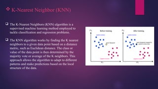
K-Nearest Neighbor(KNN)
The K-Nearest Neighbors (KNN) algorithm is a
supervised machine learning method employed to
tackle classification and regression problems.
The KNN algorithm works by finding the K nearest
neighbors to a given data point based on a distance
metric, such as Euclidean distance. The class or
value of the data point is then determined by the
majority vote or average of the K neighbors. This
approach allows the algorithm to adapt to different
patterns and make predictions based on the local
structure of the data.
39.
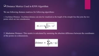
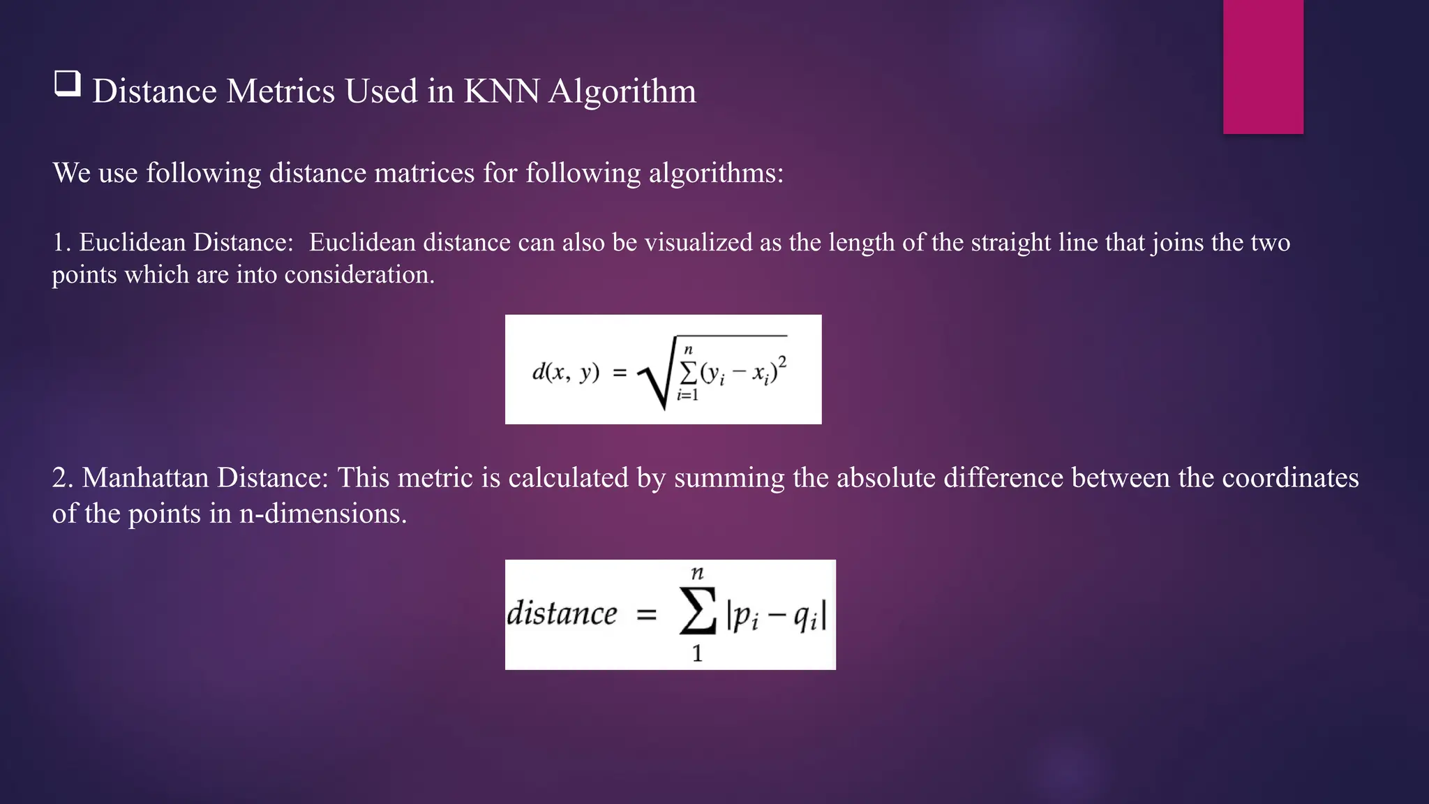
Distance MetricsUsed in KNN Algorithm
We use following distance matrices for following algorithms:
1. Euclidean Distance: Euclidean distance can also be visualized as the length of the straight line that joins the two
points which are into consideration.
2. Manhattan Distance: This metric is calculated by summing the absolute difference between the coordinates
of the points in n-dimensions.
40.
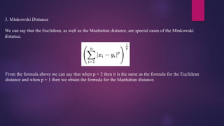
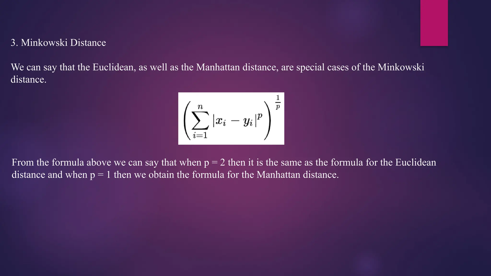
3. Minkowski Distance
Wecan say that the Euclidean, as well as the Manhattan distance, are special cases of the Minkowski
distance.
From the formula above we can say that when p = 2 then it is the same as the formula for the Euclidean
distance and when p = 1 then we obtain the formula for the Manhattan distance.
41.
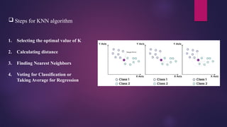
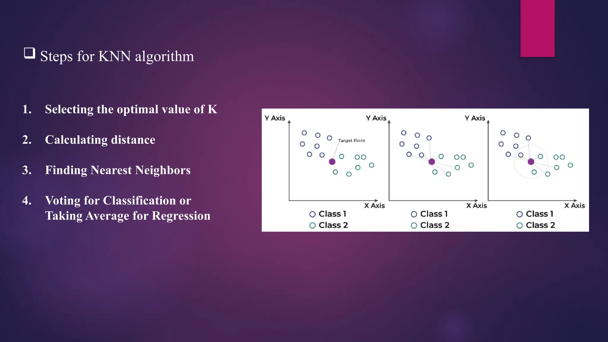
Steps forKNN algorithm
1. Selecting the optimal value of K
2. Calculating distance
3. Finding Nearest Neighbors
4. Voting for Classification or
Taking Average for Regression
42.
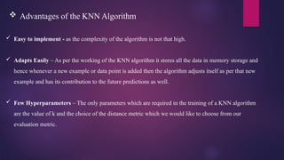
Easy toimplement - as the complexity of the algorithm is not that high.
Adapts Easily – As per the working of the KNN algorithm it stores all the data in memory storage and
hence whenever a new example or data point is added then the algorithm adjusts itself as per that new
example and has its contribution to the future predictions as well.
Few Hyperparameters – The only parameters which are required in the training of a KNN algorithm
are the value of k and the choice of the distance metric which we would like to choose from our
evaluation metric.
Advantages of the KNN Algorithm
43.
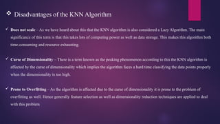
Does notscale – As we have heard about this that the KNN algorithm is also considered a Lazy Algorithm. The main
significance of this term is that this takes lots of computing power as well as data storage. This makes this algorithm both
time-consuming and resource exhausting.
Curse of Dimensionality – There is a term known as the peaking phenomenon according to this the KNN algorithm is
affected by the curse of dimensionality which implies the algorithm faces a hard time classifying the data points properly
when the dimensionality is too high.
Prone to Overfitting – As the algorithm is affected due to the curse of dimensionality it is prone to the problem of
overfitting as well. Hence generally feature selection as well as dimensionality reduction techniques are applied to deal
with this problem.
Disadvantages of the KNN Algorithm
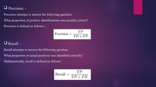
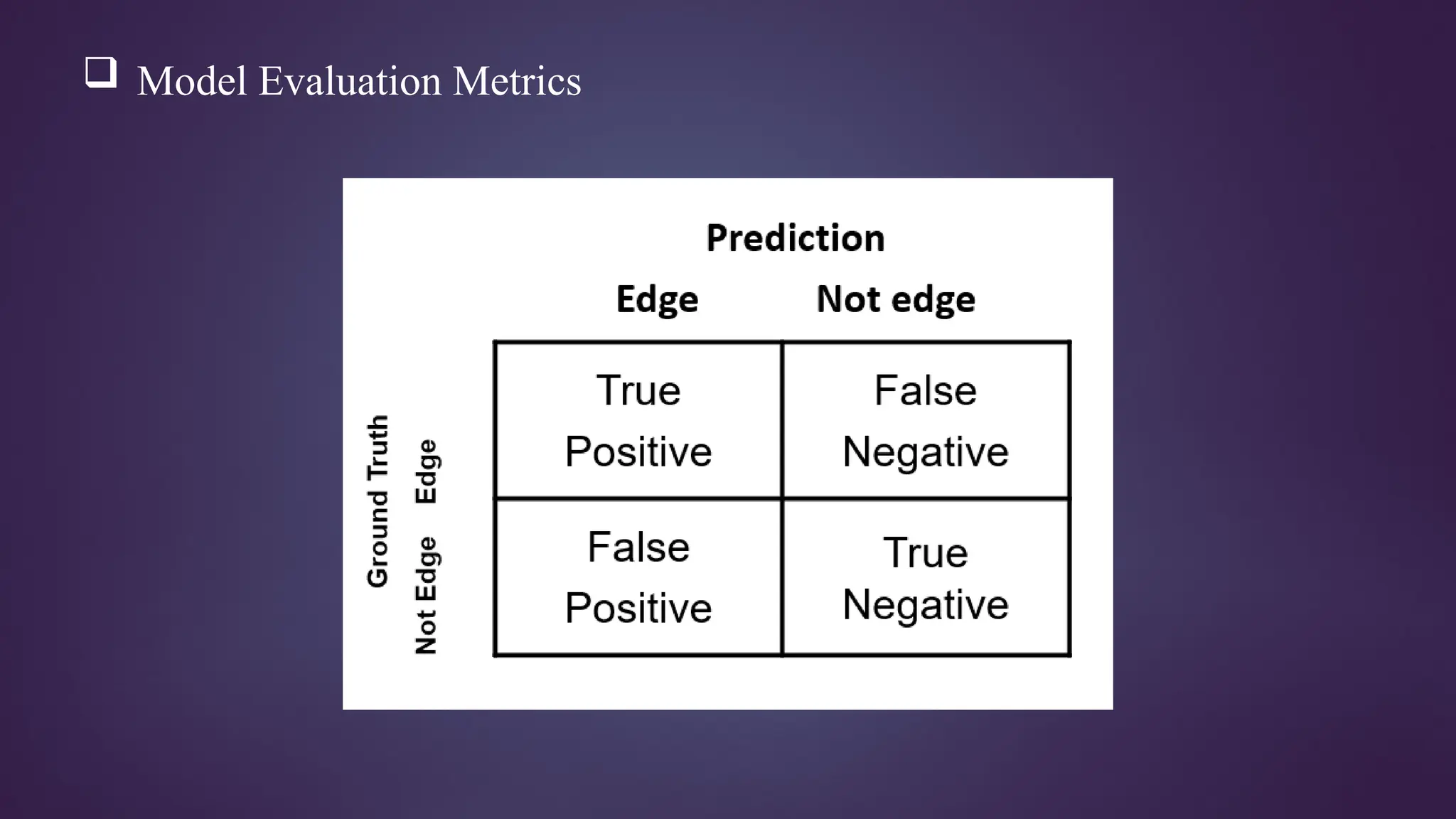
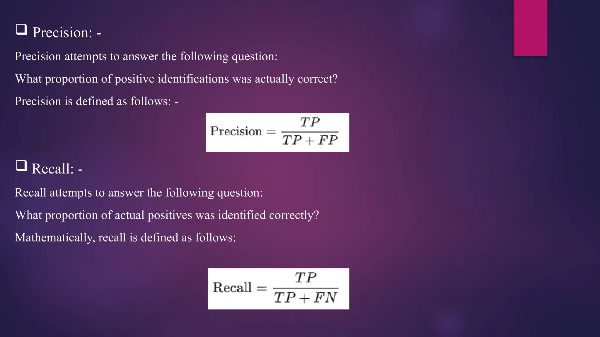
Precision: -
Precisionattempts to answer the following question:
What proportion of positive identifications was actually correct?
Precision is defined as follows: -
Recall: -
Recall attempts to answer the following question:
What proportion of actual positives was identified correctly?
Mathematically, recall is defined as follows:
46.
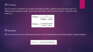
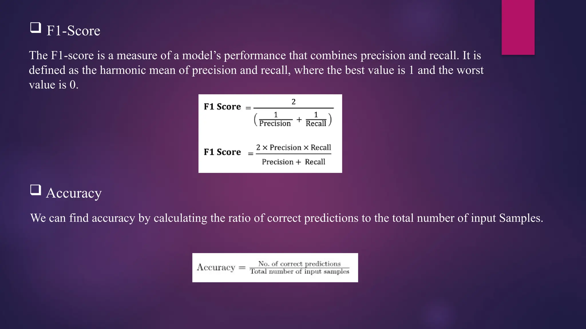
The F1-score isa measure of a model’s performance that combines precision and recall. It is
defined as the harmonic mean of precision and recall, where the best value is 1 and the worst
value is 0.
F1-Score
Accuracy
We can find accuracy by calculating the ratio of correct predictions to the total number of input Samples.
47.
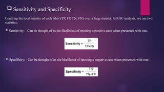
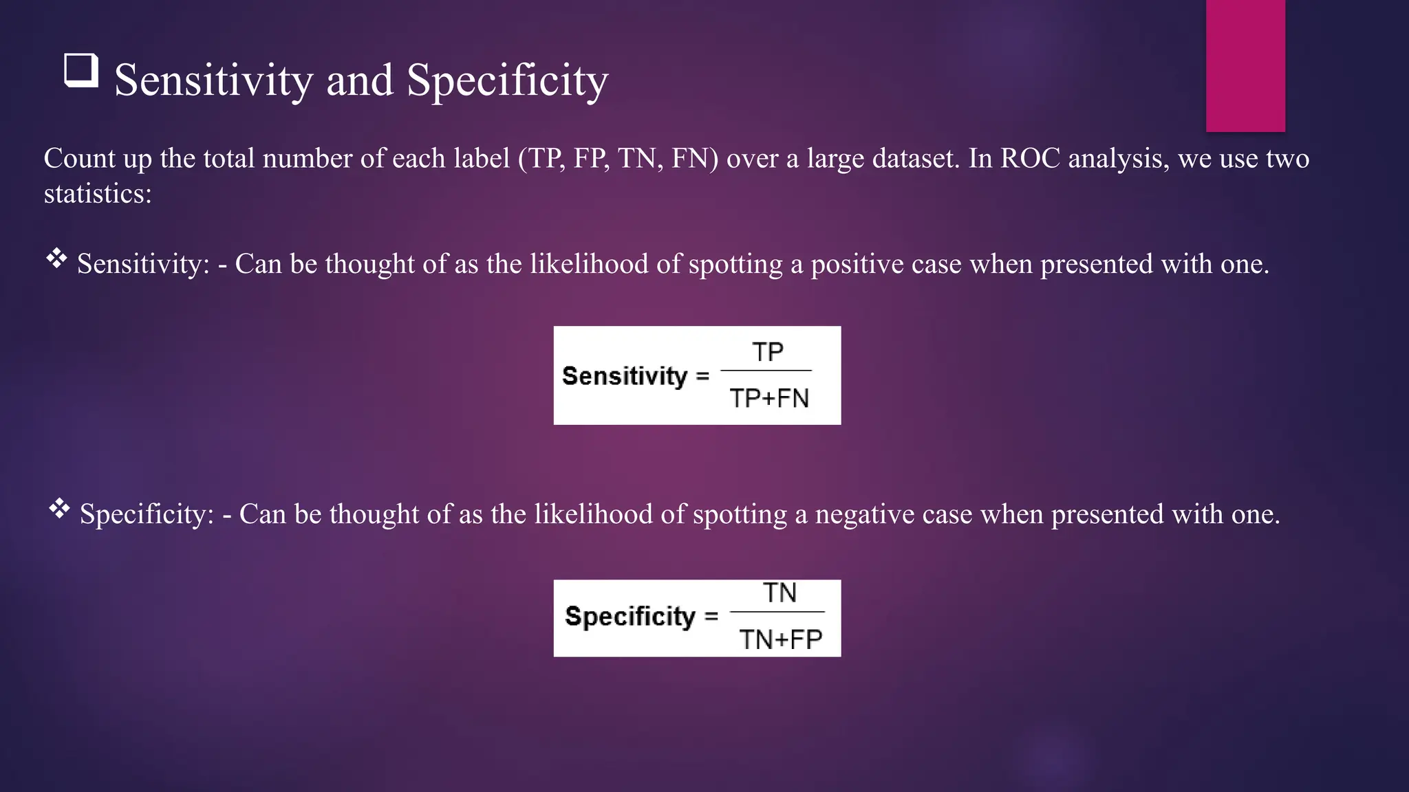
Sensitivity andSpecificity
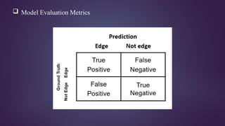
Count up the total number of each label (TP, FP, TN, FN) over a large dataset. In ROC analysis, we use two
statistics:
Sensitivity: - Can be thought of as the likelihood of spotting a positive case when presented with one.
Specificity: - Can be thought of as the likelihood of spotting a negative case when presented with one.
48.
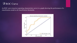
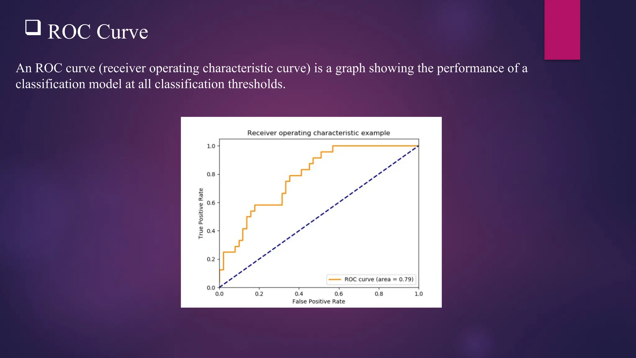
ROC Curve
AnROC curve (receiver operating characteristic curve) is a graph showing the performance of a
classification model at all classification thresholds.
49.
Unsupervised learning:-
Unsupervised learning, unlike supervised learning, does not come with labels (no output vectors).
The objective of unsupervised learning is to analyze the structure of the data and extract useful
information from it without any explicit indication of the expected result.
Unsupervised learning includes two sub-types:
1. Clustering
2. Dimensionality reduction.
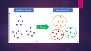
50.
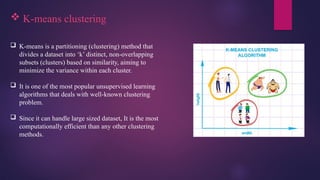
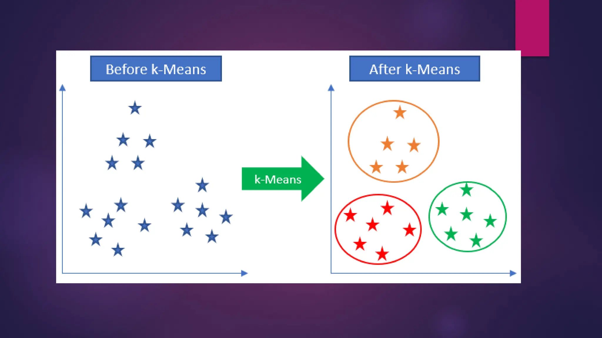
K-means clustering
K-means is a partitioning (clustering) method that
divides a dataset into ‘k’ distinct, non-overlapping
subsets (clusters) based on similarity, aiming to
minimize the variance within each cluster.
It is one of the most popular unsupervised learning
algorithms that deals with well-known clustering
problem.
Since it can handle large sized dataset, It is the most
computationally efficient than any other clustering
methods.
51.
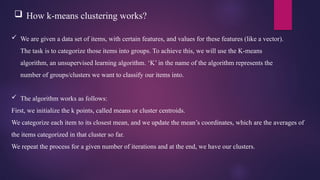
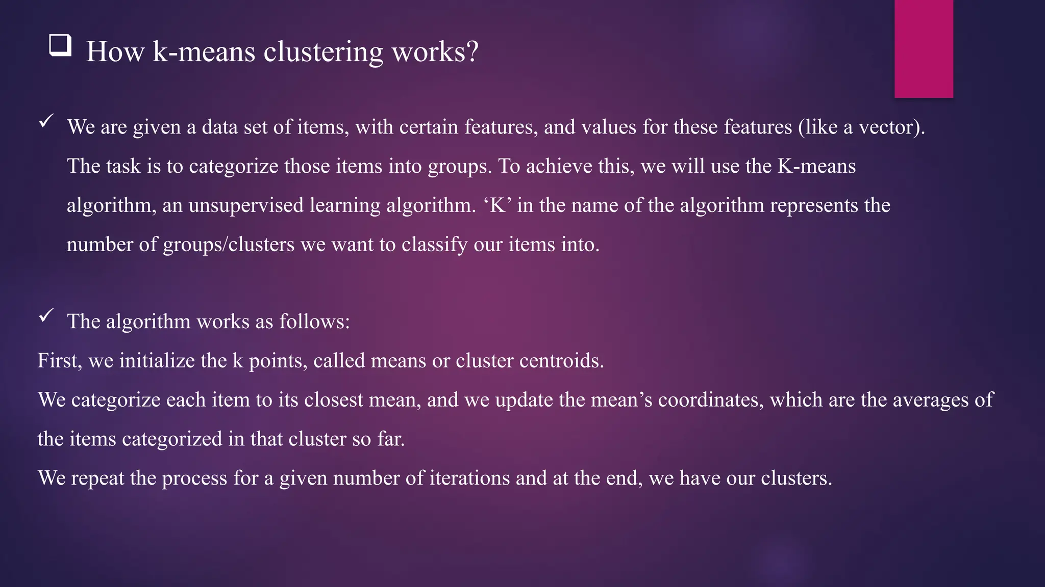
How k-meansclustering works?
We are given a data set of items, with certain features, and values for these features (like a vector).
The task is to categorize those items into groups. To achieve this, we will use the K-means
algorithm, an unsupervised learning algorithm. ‘K’ in the name of the algorithm represents the
number of groups/clusters we want to classify our items into.
The algorithm works as follows:
First, we initialize the k points, called means or cluster centroids.
We categorize each item to its closest mean, and we update the mean’s coordinates, which are the averages of
the items categorized in that cluster so far.
We repeat the process for a given number of iterations and at the end, we have our clusters.
52.
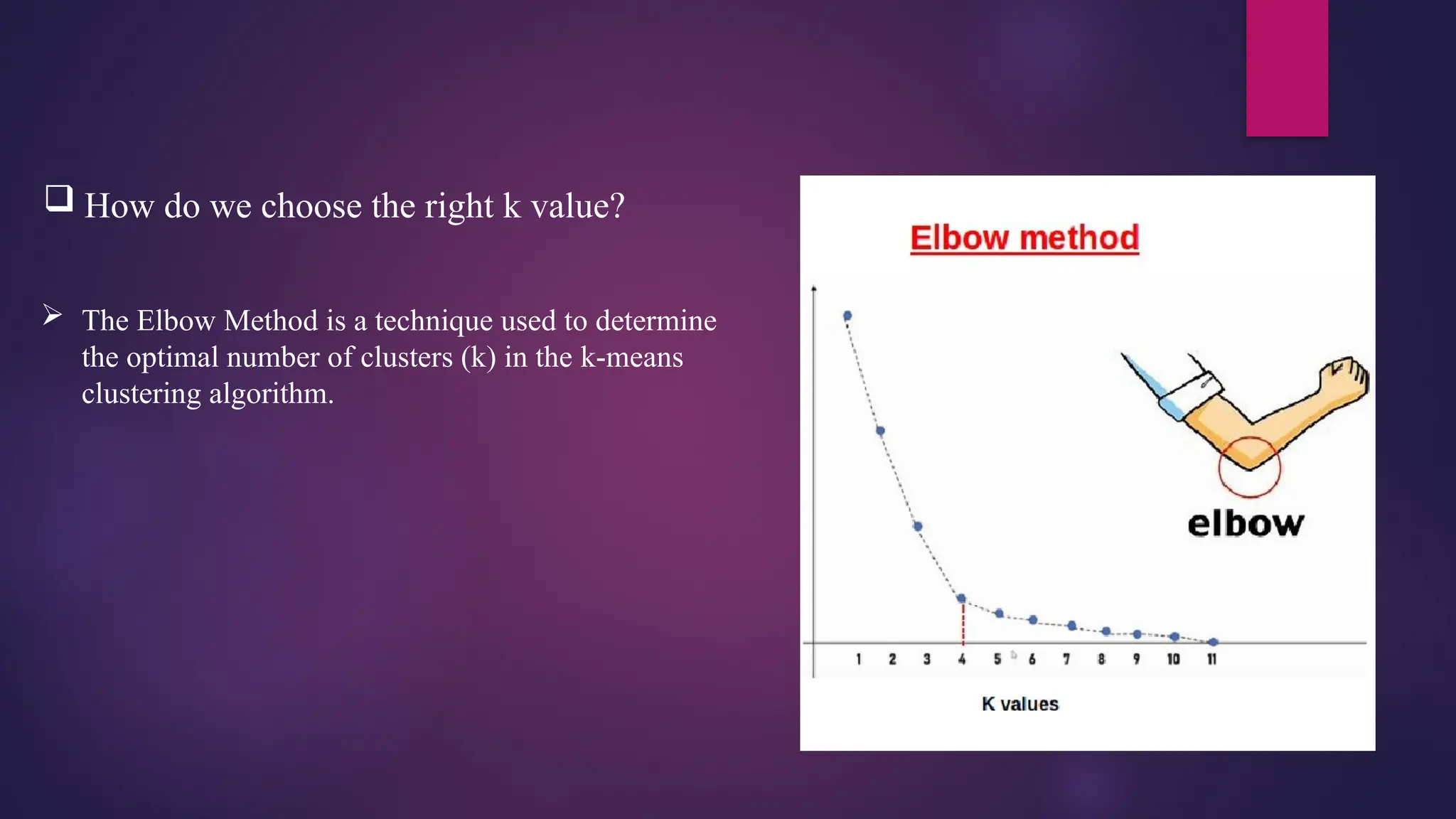
How dowe choose the right k value?
The Elbow Method is a technique used to determine
the optimal number of clusters (k) in the k-means
clustering algorithm.
53.
What doesElbow Method do?
We calculate the Within-Cluster Sum of Squares (WCSS) for different values of k.
WCSS measures the sum of square distances between the centroids and each data point.
As k increases, WCSS decreases because clusters become more compact.
However, beyond a certain point, the improvement becomes marginal.
Graphical Approach:
We plot k against its corresponding WCSS value.
The graph often resembles an “elbow.”
The optimal k value is where the graph starts to look like a straight line.
54.
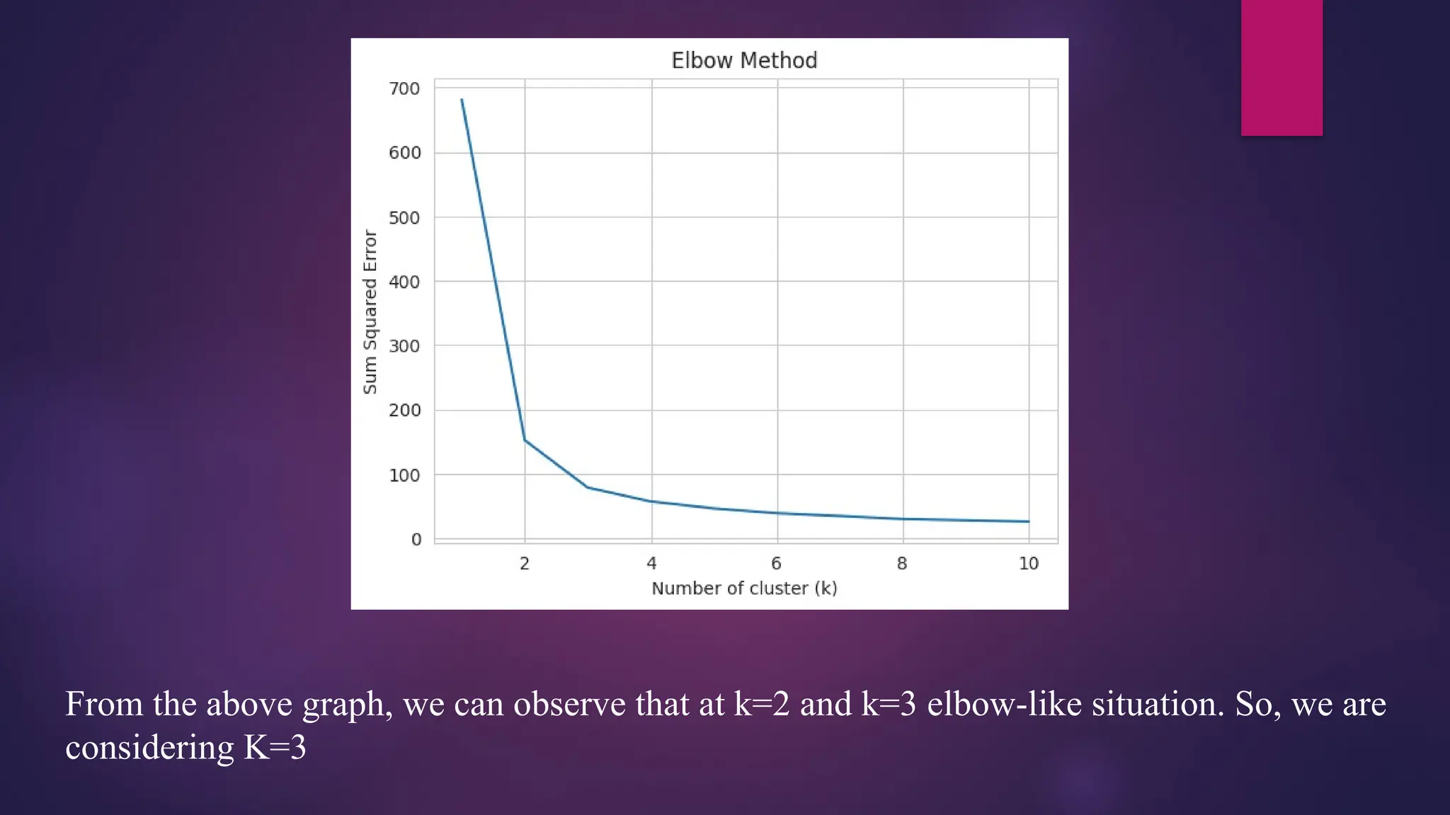
From the abovegraph, we can observe that at k=2 and k=3 elbow-like situation. So, we are
considering K=3
56.
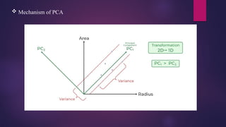
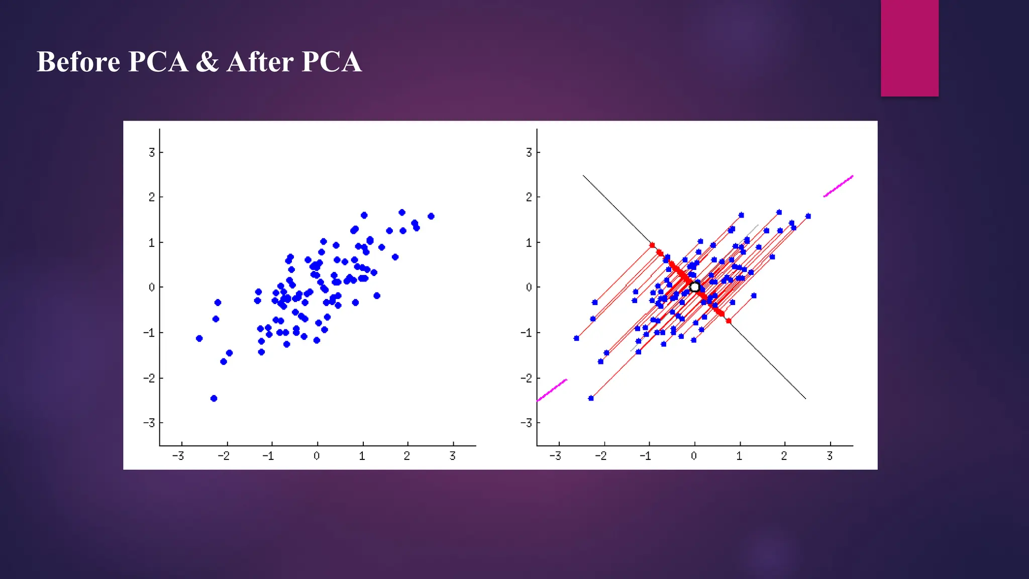
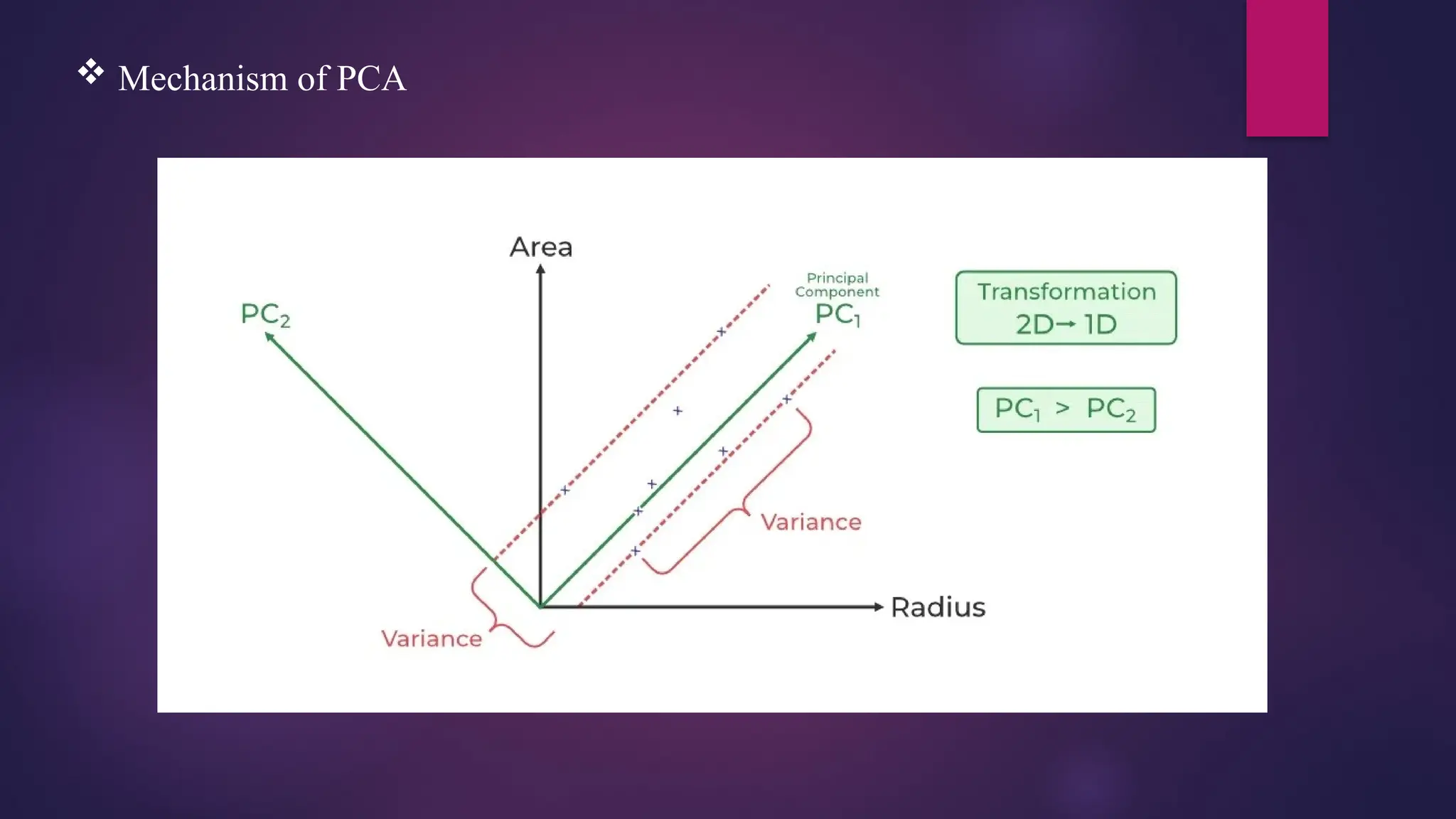
Principal ComponentAnalysis (PCA)
In modern data analysis, principal component analysis (PCA) is an essential tool as it provides a guide
for extracting the most information from a dataset, compressing the data size by keeping only those
important features without losing much information, and simplifying the description of a dataset.
It works on the condition that while the data in a higher dimensional space is mapped to data in a lower
dimension space, the variance of the data in the lower dimensional space should be maximum.
The main goal of Principal Component Analysis (PCA) is to reduce the dimensionality of a dataset while
preserving the most important patterns or relationships between the variables without any prior
knowledge of the target variables.
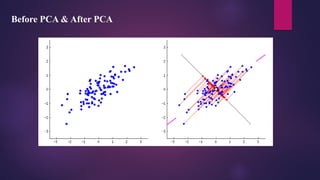
Principal ComponentAnalysis (PCA) is a technique for dimensionality reduction that
identifies a set of orthogonal axes, called principal components, that capture the maximum
variance in the data. The principal components are linear combinations of the original
variables in the dataset and are ordered in decreasing order of importance. The total variance
captured by all the principal components is equal to the total variance in the original dataset.
The first principal component captures the most variation in the data, but the second
principal component captures the maximum variance that is orthogonal to the first principal
component, and so on.
Principal Component Analysis can be used for a variety of purposes, including data
visualization, feature selection, and data compression. In data visualization, PCA can be
used to plot high-dimensional data in two or three dimensions, making it easier to interpret.
In featureselection, PCA can be used to identify the most important variables in a
dataset. In data compression, PCA can be used to reduce the size of a dataset without
losing important information.
In Principal Component Analysis, it is assumed that the information is carried in the
variance of the features, that is, the higher the variation in a feature, the more information
that features carries.
Overall, PCA is a powerful tool for data analysis and can help to simplify complex datasets,
making them easier to understand and work with.
61.
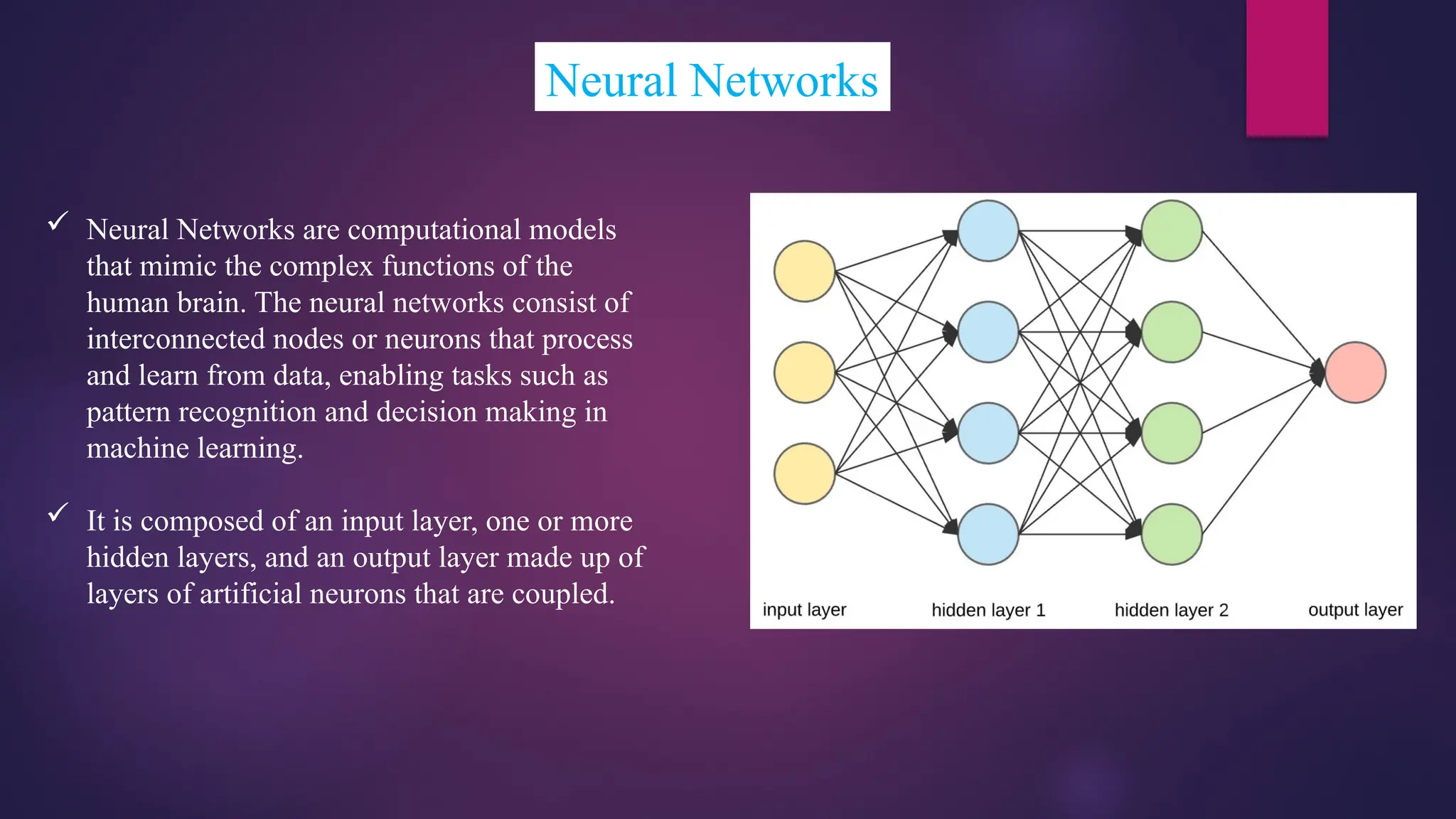
Neural Networks
NeuralNetworks are computational models
that mimic the complex functions of the
human brain. The neural networks consist of
interconnected nodes or neurons that process
and learn from data, enabling tasks such as
pattern recognition and decision making in
machine learning.
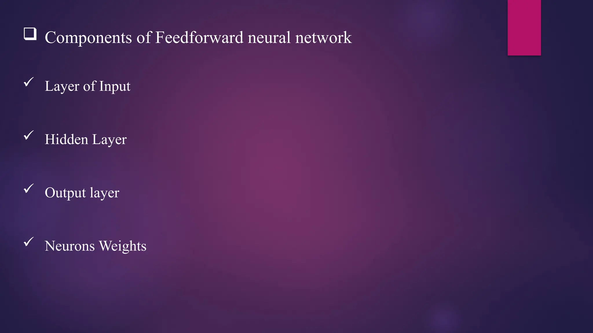
It is composed of an input layer, one or more
hidden layers, and an output layer made up of
layers of artificial neurons that are coupled.
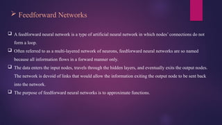
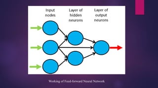
Feedforward Networks
A feedforward neural network is a type of artificial neural network in which nodes’ connections do not
form a loop.
Often referred to as a multi-layered network of neurons, feedforward neural networks are so named
because all information flows in a forward manner only.
The data enters the input nodes, travels through the hidden layers, and eventually exits the output nodes.
The network is devoid of links that would allow the information exiting the output node to be sent back
into the network.
The purpose of feedforward neural networks is to approximate functions.
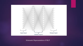
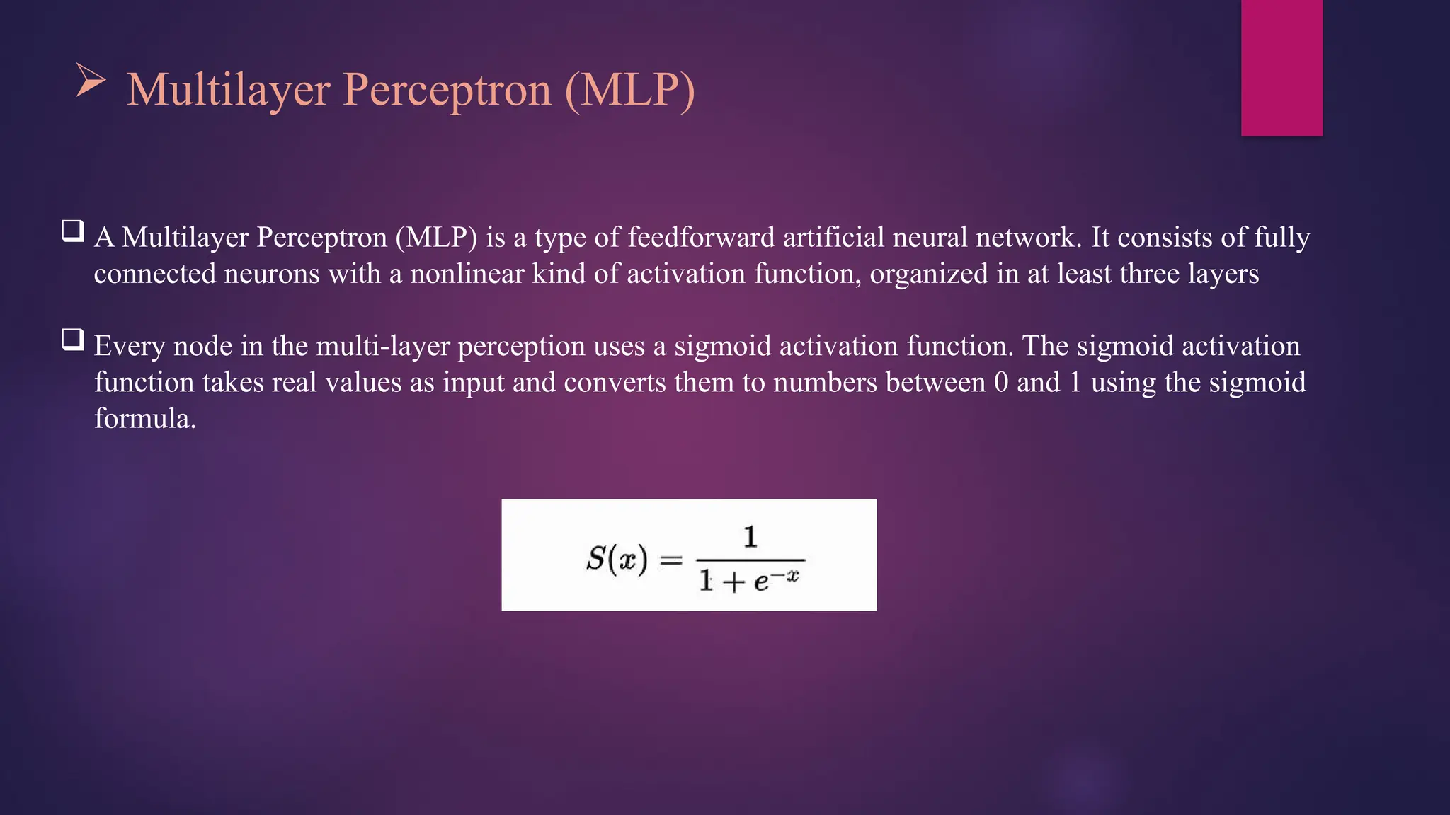
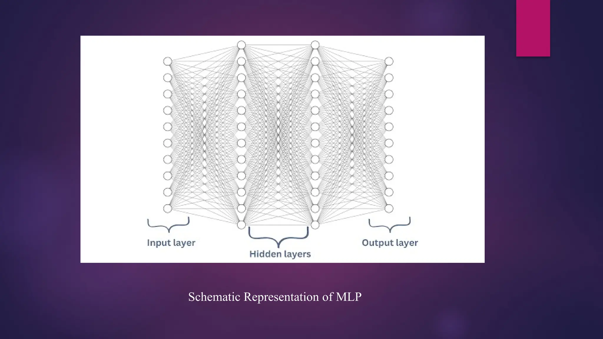
Multilayer Perceptron(MLP)
A Multilayer Perceptron (MLP) is a type of feedforward artificial neural network. It consists of fully
connected neurons with a nonlinear kind of activation function, organized in at least three layers
Every node in the multi-layer perception uses a sigmoid activation function. The sigmoid activation
function takes real values as input and converts them to numbers between 0 and 1 using the sigmoid
formula.
Multilayer Perceptronfalls under the category of feedforward algorithms, because inputs are
combined with the initial weights in a weighted sum and subjected to the activation function, just
like in the Perceptron. But the difference is that each linear combination is propagated to the next
layer.
Multi-layer perceptrons (MLPs) have a wide range of applications in various fields like, in Image
classification, Speech recognition, Natural language Processing, Finance, Computer vision,
Machine translation etc.
69.
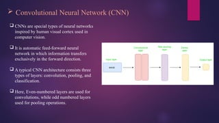
Convolutional NeuralNetwork (CNN)
CNNs are special types of neural networks
inspired by human visual cortex used in
computer vision.
It is automatic feed-forward neural
network in which information transfers
exclusively in the forward direction.
A typical CNN architecture consists three
types of layers: convolution, pooling, and
classification.
Here, Even-numbered layers are used for
convolutions, while odd numbered layers
used for pooling operations.
70.
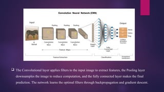
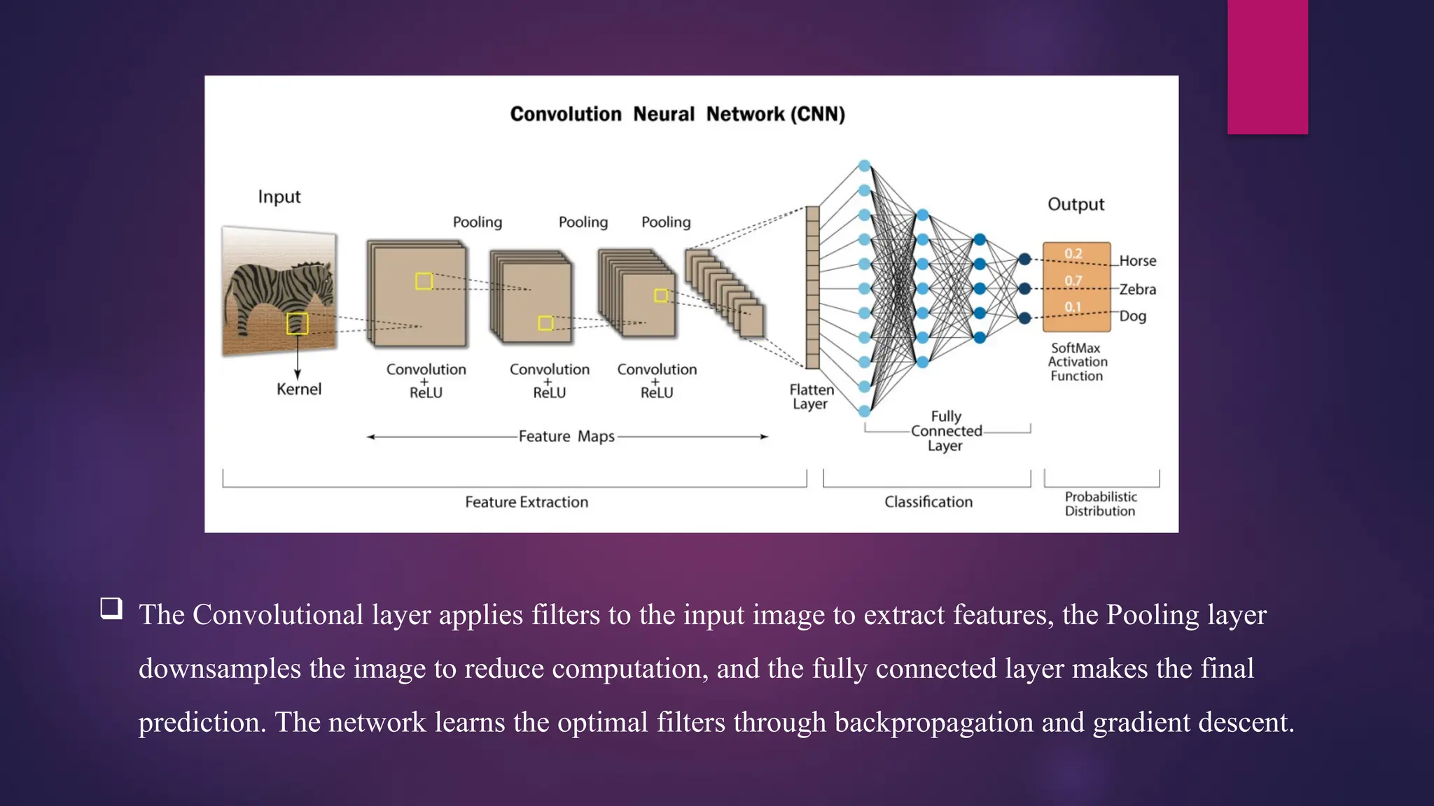
The Convolutionallayer applies filters to the input image to extract features, the Pooling layer
downsamples the image to reduce computation, and the fully connected layer makes the final
prediction. The network learns the optimal filters through backpropagation and gradient descent.
71.
Advantages of ConvolutionalNeural Networks (CNNs):
Good at detecting patterns and features in images, videos, and audio signals.
Robust to translation, rotation, and scaling invariance.
End-to-end training, no need for manual feature extraction.
Can handle large amounts of data and achieve high accuracy.
Disadvantages of Convolutional Neural Networks (CNNs):
Computationally expensive to train and require a lot of memory.
Can be prone to overfitting if not enough data or proper regularization is used.
Requires large amounts of labeled data.
Interpretability is limited, it’s hard to understand what the network has learned.
72.
Recurrent NeuralNetwork (RNN)
Recurrent Neural Network (RNN) is a type of Neural Network where the output from the previous
step is fed as input to the current step.
In traditional neural networks, all the inputs and outputs are independent of each other. Still, in cases
when it is required to predict the next word of a sentence, the previous words are required and hence
there is a need to remember the previous words. Thus RNN came into existence, which solved this
issue with the help of a Hidden Layer.
The main and most important feature of RNN is its Hidden state, which remembers some information
about a sequence. The state is also referred to as Memory State since it remembers the previous input
to the network. It uses the same parameters for each input as it performs the same task on all the
inputs or hidden layers to produce the output. This reduces the complexity of parameters, unlike other
neural networks.
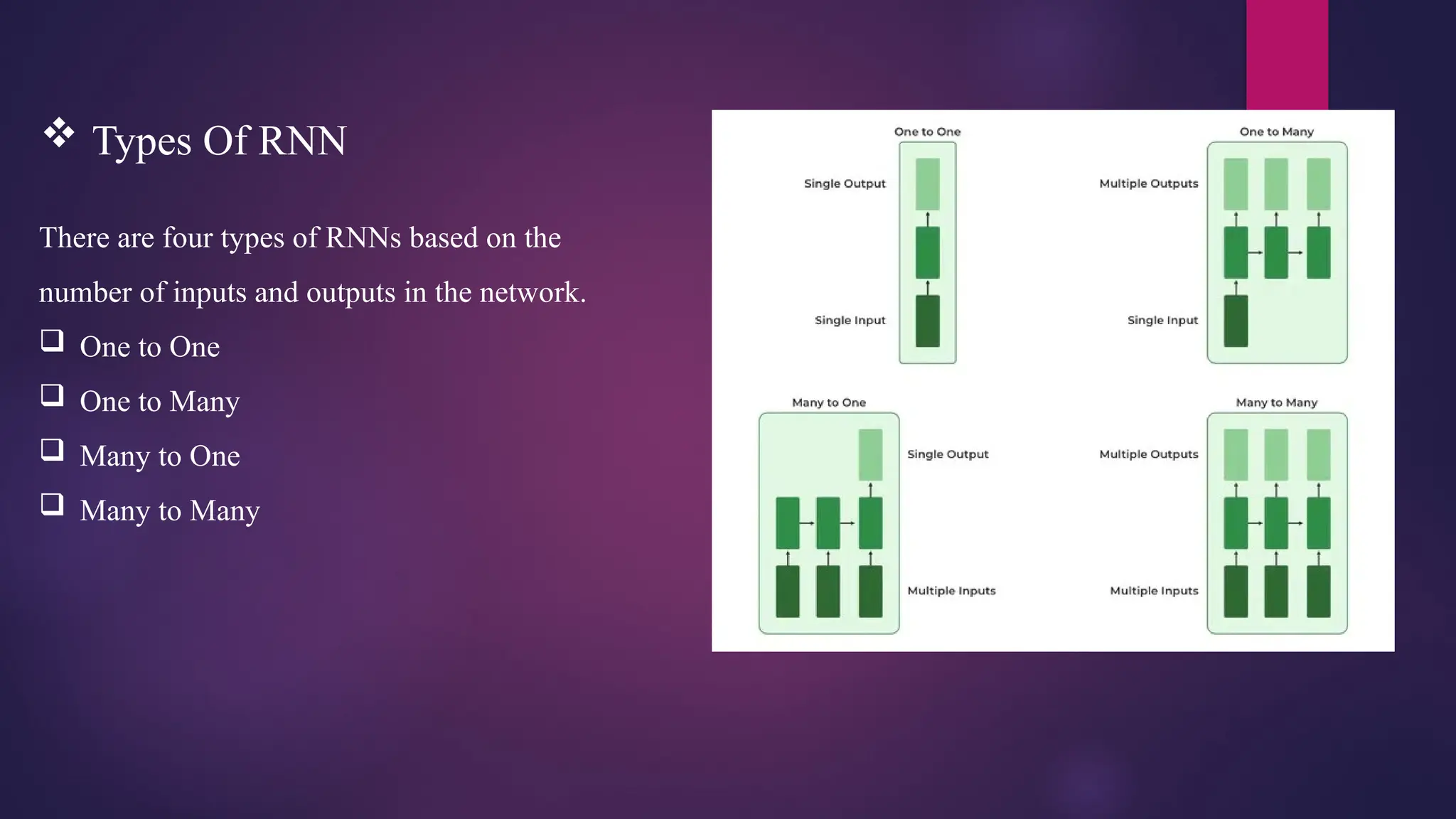
Types OfRNN
There are four types of RNNs based on the
number of inputs and outputs in the network.
One to One
One to Many
Many to One
Many to Many
75.
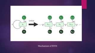
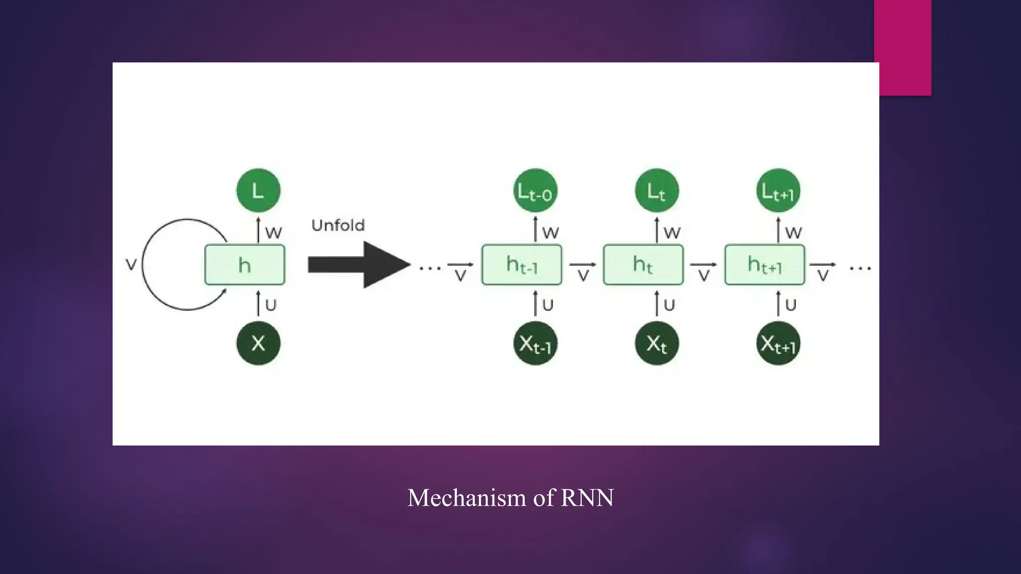
How doesRNN work?
The Recurrent Neural Network consists of multiple fixed activation function units, one for
each time step. Each unit has an internal state which is called the hidden state of the unit. This
hidden state signifies the past knowledge that the network currently holds at a given time
step. This hidden state is updated at every time step to signify the change in the knowledge of
the network about the past.
Applications of Recurrent Neural Network
• Language Modelling and Generating Text
• Speech Recognition
• Machine Translation
• Image Recognition, Face detection
• Time series Forecasting
76.
Long Short-TermMemory (LSTM)
LSTM networks are an extension of recurrent neural networks (RNN’s) mainly introduced to
handle situations where RNNs fail.
It fails to store information for a longer period of time. At times, a reference to certain
information stored quite a long time ago is required to predict the current output. But RNNs
are absolutely incapable of handling such “long-term dependencies”.
There is no finer control over which part of the context needs to be carried forward and how
much of the past needs to be ‘forgotten’.
Other issues with RNNs are exploding and vanishing gradients which occur during the
training process of a network through backtracking.
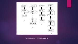
Figure-A representswhat a basic LSTM network looks like. Only one layer of LSTM between an input
and output layer has been shown here.
Figure B represents Deep LSTM which includes a number of LSTM layers in between the input and
output. The advantage is that the input values fed to the network not only go through several LSTM
layers but also propagate through time within one LSTM cell. Hence, parameters are well distributed
within multiple layers. This results in a thorough process of inputs in each time step.
Figure C represents LSTM with the Recurrent Projection layer where the recurrent connections are taken
from the projection layer to the LSTM layer input. This architecture was designed to reduce the high
learning computational complexity (O(N)) for each time step) of the standard LSTM RNN.
79.
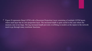
Figure Drepresents Deep LSTM with a Recurrent Projection Layer consisting of multiple LSTM layers
where each layer has its own projection layer. The increased depth is quite useful in the case where the
memory size is too large. Having increased depth prevents overfitting in models as the inputs to the network
need to go through many nonlinear functions.
Drawback ofLSTM Networks
Problem of vanishing gradients
Sometimes Inefficient
Different random weight initialization
More expectations required
82.
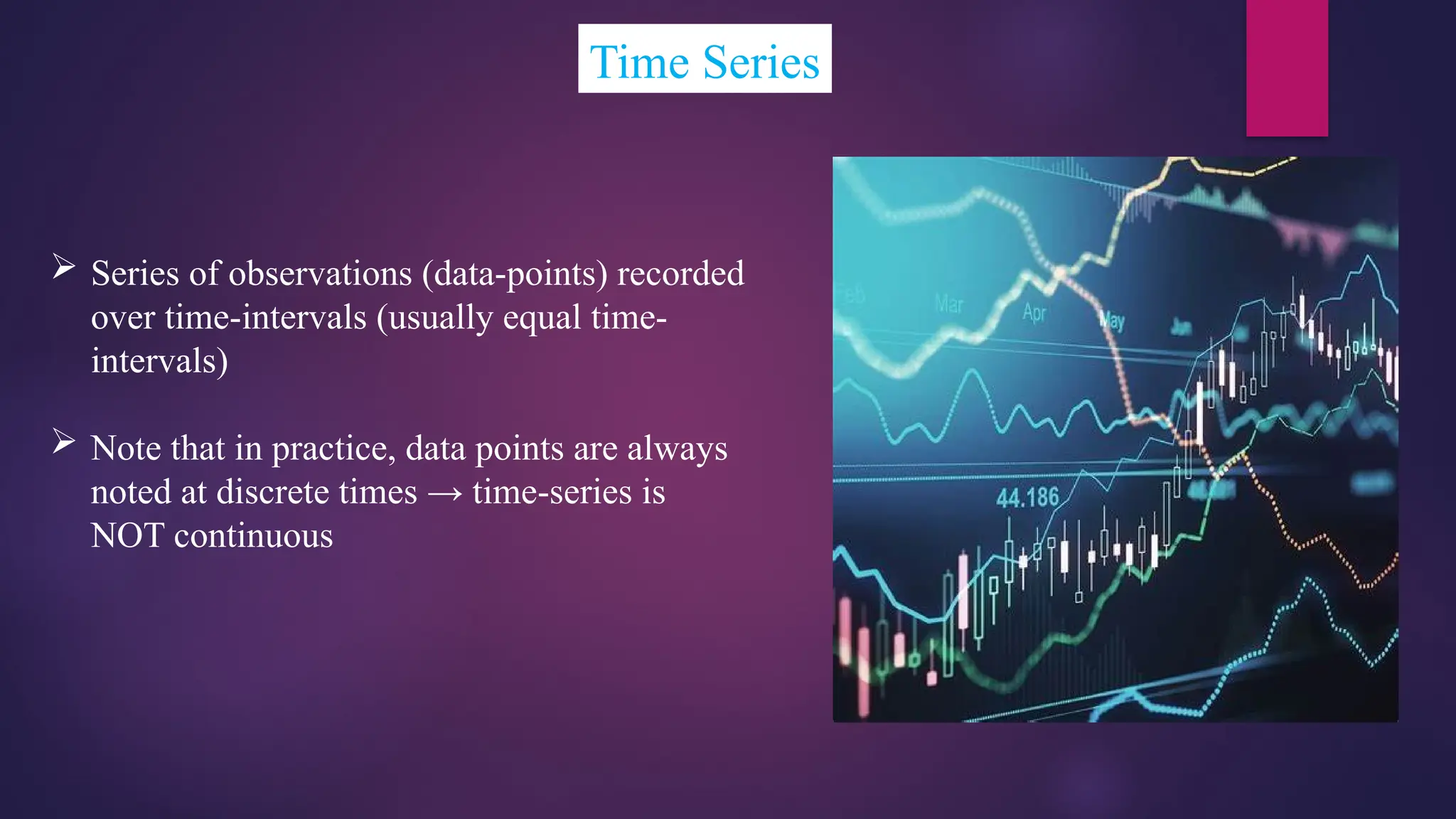
Time Series
Seriesof observations (data-points) recorded
over time-intervals (usually equal time-
intervals)
Note that in practice, data points are always
noted at discrete times → time-series is
NOT continuous
83.
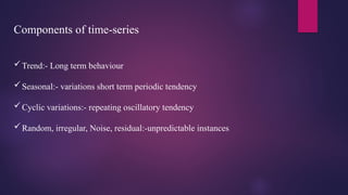
Components of time-series
Trend:-Long term behaviour
Seasonal:- variations short term periodic tendency
Cyclic variations:- repeating oscillatory tendency
Random, irregular, Noise, residual:-unpredictable instances
84.
Auto Regressivemodels (AR Model)
Self
Relation between two variables
predicting value of one variable to another variable
“So, Basically AR model is Predict future values from past self values”
85.
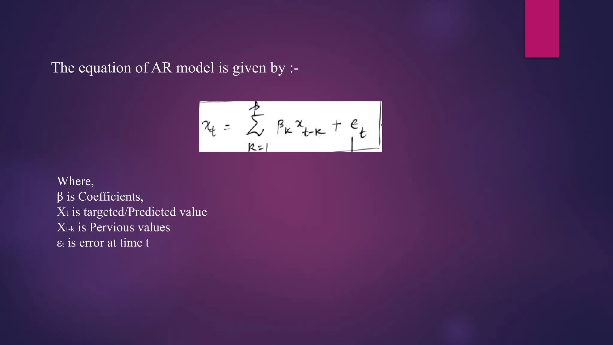
The equation ofAR model is given by :-
Where,
β is Coefficients,
Xt is targeted/Predicted value
Xt-k is Pervious values
εt is error at time t
86.
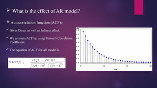
What isthe effect of AR model?
Autocorrelation function (ACF):-
Gives Direct as well as Indirect effect.
We estimate ACF by using Person’s Correlation
Coefficient.
The equation of ACF for AR model is
87.
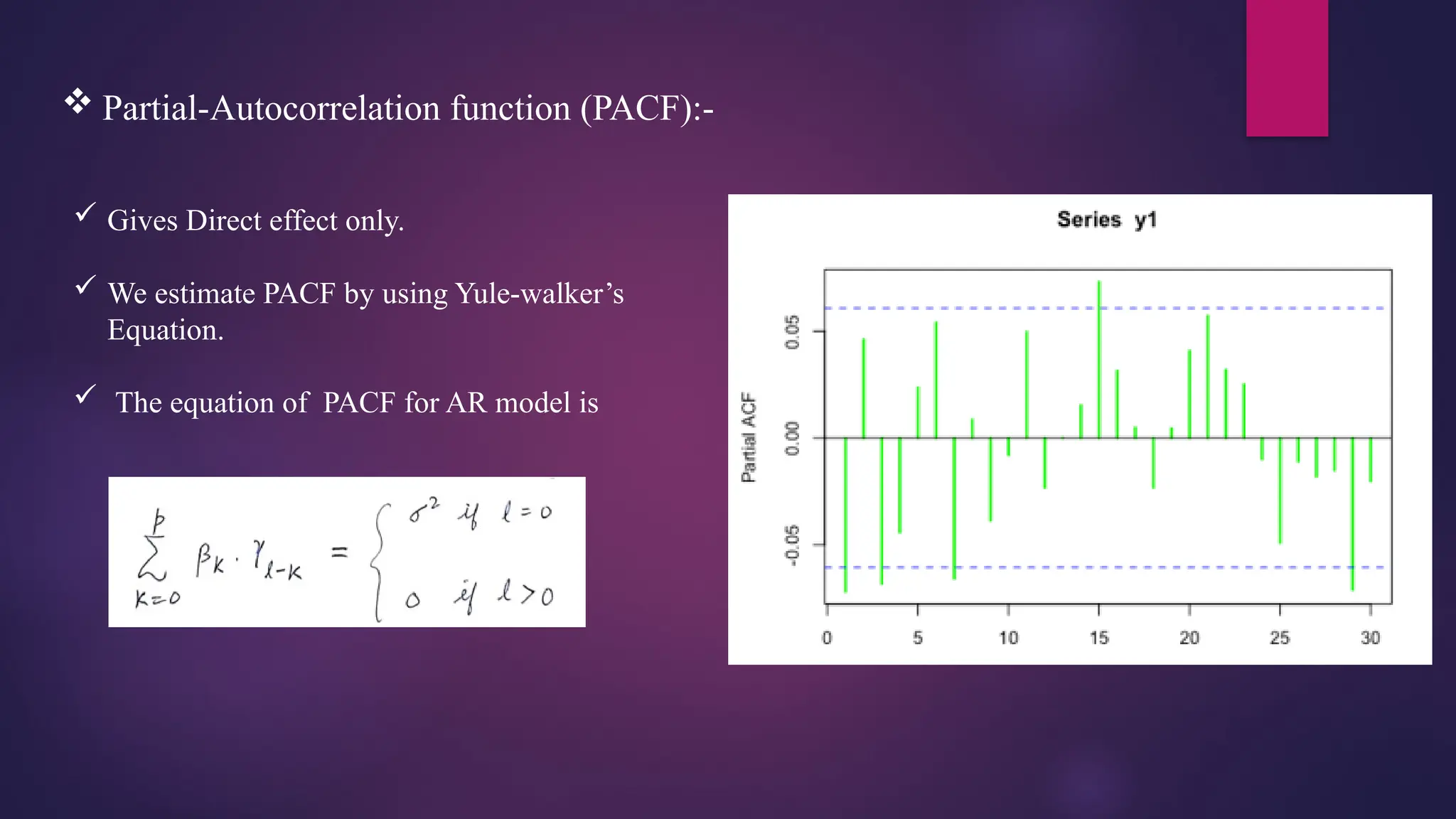
Partial-Autocorrelation function(PACF):-
Gives Direct effect only.
We estimate PACF by using Yule-walker’s
Equation.
The equation of PACF for AR model is
88.
Applications ofAuto-Regressive model
Benefits of Autoregressive Models:
Simplicity: AR models are relatively simple to understand and implement. They rely on past values of
the time series to predict future values, making them conceptually straightforward.
Interpretability: The coefficients in an AR model have clear interpretations. They represent the
strength and direction of the relationship between past and future values, making it easier to derive
insights from the model.
Useful for Stationary Data: AR models work well with stationary time series data. Stationary data
have stable statistical properties over time, which is an assumption that AR models are built upon.
Efficiency: AR models can be computationally efficient, especially for short time series or when you
have a reasonable amount of data.
89.
Drawbacks of AutoregressiveModels:
Stationarity Assumption: AR models assume that the time series is stationary, meaning that its statistical
properties do not change over time. In practice, many real-world time series are non-stationary, requiring
preprocessing steps like differencing.
Limited to Short-Term Dependencies: AR models are not well-suited for capturing long-term dependencies
in data. They are primarily designed for modeling short-term temporal patterns.
Lag Selection: Choosing the appropriate lag order (p) in an AR model can be challenging. Selecting too few
lags may lead to underfitting, while selecting too many may lead to overfitting. Techniques like ACF and
PACF plots are used to determine the lag order.
Sensitivity to Noise: AR models can be sensitive to random noise in the data. This sensitivity can lead to
overfitting, especially when dealing with noisy or irregular time series.


![Agentic Systems and Compliance - A brief intro [1.2]](https://cdn.slidesharecdn.com/ss_thumbnails/agenticsystemsandcompliace-1-251018025303-958a42ec-thumbnail.jpg?width=600ounds&width=560&fit=bounds)


