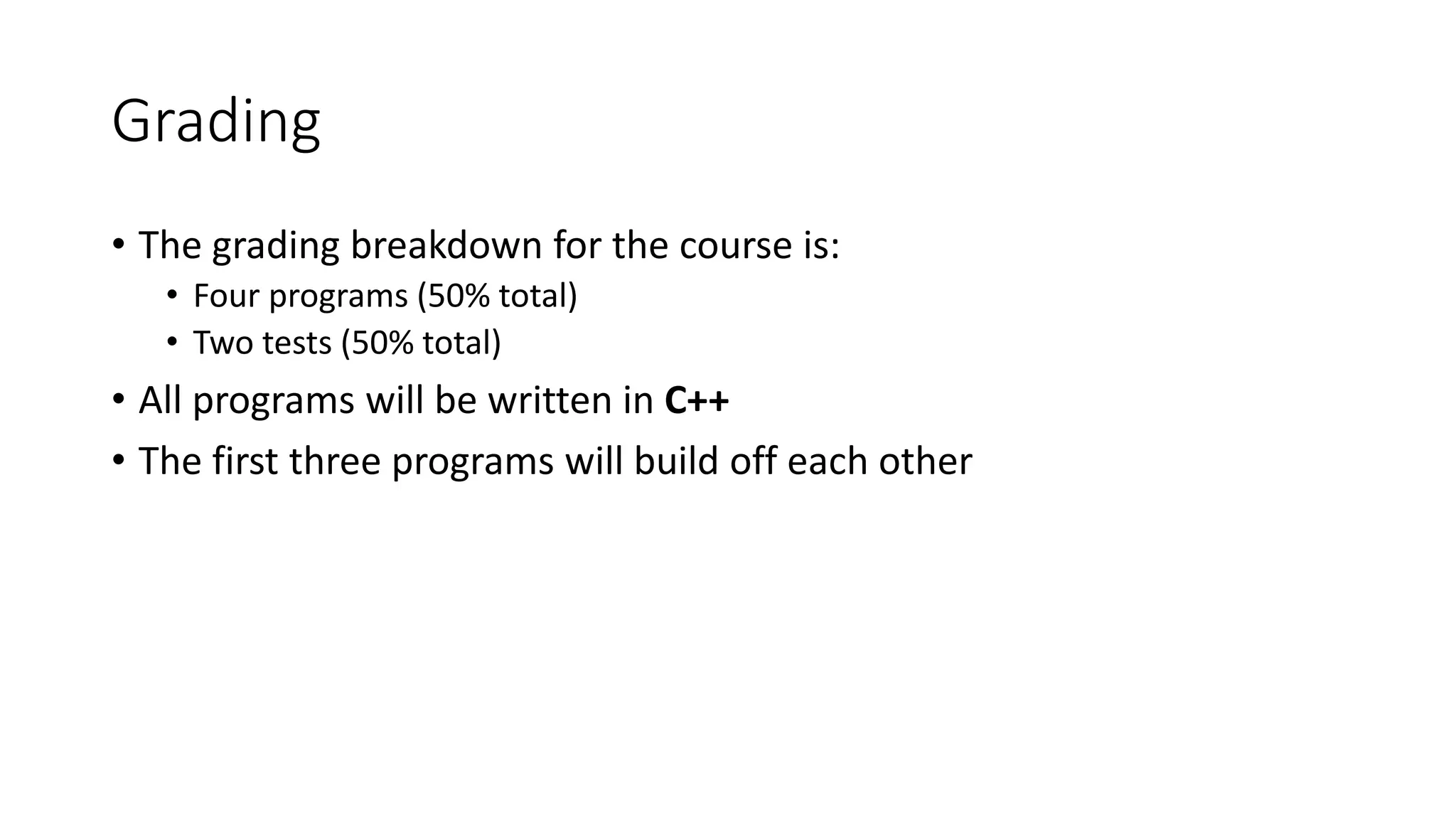
KEMBAR78
Review to the data structure and algorithm | PPTX
ECE365: Data Structures and
Algorithms II (DSA 2)
Course Intro and Review of DSA 1
The Basics
• Lectures will be in person, Wednesdays 4 pm – 6 pm in Rm. 505
• If we are forced to be remote at any point during the semester, those
lectures will take place via Teams
• My webpage: http://faculty.cooper.edu/sable2
• From there, you can fine a link to the course webpage
• I’ll post syllabus info and assignments on the course webpage
• My email: carl.sable@cooper.edu
The Textbook
• “Data Structures and Algorithm Analysis in C++” by Mark Allen Weiss
• I recommend the 4th Edition (updated for C++11)
• This is the same book that was used for DSA 1
• Other references (not required):
• “Algorithms”, by Sedgewick, the 3rd edition
• “Introduction to Algorithms”, the 3rd edition, by Cormen, Leiserson, Rivest,
and Stein
Grading
• The grading breakdown for the course is:
• Four programs (50% total)
• Two tests (50% total)
• All programs will be written in C++
• The first three programs will build off each other
What are Data Structures and Algorithms?
• Informal definitions:
• Data structures are constructs for organizing data
• Algorithms are methods of solving a problem
• Or: An algorithm is a well-defined sequence of computational steps that
transforms structured input into structured output
• We will see a more formal definition of an algorithm near the end of
this course
Helpful Notations for Analyzing Algorithms
• Big-O (a.k.a. Big-Oh): T(N) = O(f(N)) if there exist positive constants c and n0
such that T(N) ≤ c*f(N) when N >= n0
• Big-Omega (a.k.a. Omega): T(N) = Ω(g(N)) if there exist positive constants c
and n0 such that T(N) ≥ c*g(N) when N ≥ n0
• Big-Theta (a.k.a. Theta): T(N) = Θ(h(N)) if and only if T(N) = O(h(N)) and
T(N) = Ω(h(N))
• We also covered Little-O, but that is less commonly used
• Typically, we use these notations to analyze the worst-case running time
(really, the number of computational steps) of an algorithm
• Sometimes we analyze the average-case running time or the memory
requirements of an algorithm
Analyzing Pseudo-code or Code
• We covered a series of mathematical rules applying to Big-O or the related
notations
• Example: if T(N) is a polynomial of degree k, then T(N) = Θ(Nk)
• We also went over a series of rules that tell us how to use these notations to
analyze pseudo-code
• Example: work inside out and multiply when you are dealing with nested loops
• We also covered the Master Theorem which allows us to analyze certain
recurrences that occur when we analyze some recursive algorithms
• We analyzed various solutions to the Maximum Subsequence Sum Problem
• We saw that algorithms with different Big-O running times take vastly different
actual times to run
• We also explained why exponential running time algorithms are even much worse
than high-order polynomial time algorithms
Overview of Overview of C++ (not a typo)
• DSA 1 included an overview of C++
• Concepts covered included streams, strings, pointers, dynamic
memory, references, exception handling, overloaded functions, etc.
• We discussed object-oriented programming in C++
• Concepts covered include classes, objects, encapsulation, information
hiding, operator overloading, inheritance, polymorphism, etc.
• We also covered C++ templates, which allows generic programming
Lists
• We discussed the notion of an abstract data type (ADT); this defines the values
that can be stored and the types of operations that can be applied to the values
• An abstract data type does not imply how the actual data type is to be
implemented
• We discussed the list abstract data type, and discussed advantages and
disadvantages of implementing an array-based list vs. a linked list
• Arrays allow a constant time findKth operation, but require linear time for
insertion and deletion since existing elements need to be shifted
• Linked lists allow constant time insertions and deletions (given access to the
previous node), but findKth becomes a linear operation
• C++ provides a vector class that supports resizable arrays, and a list class that
provides doubly linked list functionality (both implementations rely on templates)
Stacks and Queues
• We covered stacks and queues, two simple but very important ADTs
• I tend to think of a stack as a closed bucket and a queue as an open pipe
• You can insert into either data structure using a push or delete using a pop; most
modern sources prefer the terms enqueue and dequeue when dealing with a queue
• A stack uses a LIFO strategy, and a queue uses a FIFO strategy
• Both stacks and queues can be implemented with arrays or linked lists
• One of your programming assignments involved linked lists, stacks, and queues; the
implementation required the use of classes, inheritance, polymorphism, and templates
• We covered at least a couple of linear algorithms that use stacks; e.g., an algorithm for
checking if an expression containing left- and right-markers is balanced
• We also discussed how every program you write with function calls relies on a call stack
(a.k.a. the stack) of activation records; without this, recursion would not be possible
Trees
• We covered was trees, starting with terminology; e.g., root, leaf,
internal node, child, parent, ancestor, descendant, depth, etc.
• Three traversal strategies, generally implemented with recursion, are
preorder traversal, postorder traversal, and inorder traversal
• Another traversal strategy, generally implemented using a queue, is
breadth-first search
• In a binary tree, every node can have at most two children
Binary Search Trees
• A binary search tree is a binary tree that constrains the ordering of nodes
based on their keys
• Binary search trees support average-case logarithmic time insertion and search
• Items can be traversed in sorted order (according to keys) in linear time using an
inorder traversal
• An ordinary binary search tree has worst-case linear insertion and search
• An AVL tree is one type of balanced binary search tree that guarantees
worst-case logarithmic time insertions and searches
• For each node, v, of an AVL tree, T, the heights of the two subtrees of v must differ by
at most 1
• We saw how this property can be maintained without violating logarithmic time
insertion by using single rotations and double rotations
• Other types of balanced trees include splay trees, red black trees, and B+
trees (not binary)
Sorting and Simple Sorts
• We spent a few weeks covering sorting algorithms
• Some of the sorts we covered are stable, meaning that items with
equal keys remain in the same relative order before and after the sort
• Three simple, quadratic-time sorts are bubble sort, selection sort, and
insertion sort
• Bubble sort and insertion sort can be very fast for sequences that
start off in close-to-sorted order
Θ(N log N) Sorting Algorithms
• Two Θ(N log N) sorts that we covered in detail are mergesort and quicksort
• Both sorts typically rely on recursion and use a divide-and-conquer strategy
• Mergesort sorts the left half of the sequence, then sorts the right half of
the sequence, them merges the two sorted halves together
• Quicksort relies on a partition, which uses a pivot; a common strategy for
choosing a pivot is called median-of-three partitioning
• Quicksort is one of the fastest general sorting algorithms in practice
• Most implementations of quicksort are Θ(N2) in the worst case, but this is
exponentially unlikely with a good implementation
• Quicksort is not a stable sort, whereas mergesort is stable
Linear Sorting Algorithms
• We proved that O(N log N) is the best you can do for any comparison-
based sort
• Bin sort (a.k.a. bucket sort or counting sort) is a linear time sort, but it
makes very strict assumptions about the possible data
• (Least-significant-digit) radix sort is an extension of this type of sort
that makes less strict assumptions about the data
• For example, radix sort it can be used to sort 32-bit integers and still
provides a linear time sort
Indirect Sorting
• If you are sorting very large structures, or items in a linked list, it
might be helpful to use indirect sorting
• Two methods of indirect sorting are a pointer sort or an index sort
(the latter cannot be applied to link lists)
• If an in-place sort is necessary, you can follow an indirect sort with
another routine to move items into their correct locations
Hash Tables and Hash Functions
• The last topic we covered was hash tables
• Hash tables typically support two or three operations: insert, search, and
(possibly) delete
• The goal of a hash table is to provide the supported operations in constant
average time
• A hash table typically makes use of a large array; it is often advisable to
make the size of the array a prime number
• A hash table implementation must rely on a hash function which maps a
key (often a string) to a slot in the hash table
• A modular hash function, as its last step, takes the remainder when some
calculated number is divided by the size of the hash table
Collisions and Collision Resolution Strategies
• A collision occurs when non-equal keys get mapped by the hash function to
the same location
• When this happens, the hash table must rely on a collision resolution
strategy
• The simplest collision resolution strategy is separate chaining, in which each slot
stores a linked list of items that hash to that slot
• For separate chaining, the load factor represents the average size of each list
• Two other commonly used collision resolution strategies are linear probing and
double hashing; these are examples of open addressing schemes
• For these strategies, the load factor is the fraction of the table that is occupied, and
it must be less than 1 (typically you want to keep it much lower; e.g., less than 0.5)
• Open addressing schemes are more complicated and only support lazy deletion;
however, they allow faster operations by avoiding dynamic memory allocation
Rehashing
• It is typically a good idea to keep the load factor small (e.g., less then
0.5), especially for the open addressing schemes
• One way to ensure this is with rehashing, which resizes the hash table
when it fills to a certain point
• Everything from the original table gets reinserted into the new, larger table
• When you rehash, you eliminate the lazily deleted items
• Although this will mean that occasionally there will be a relatively
slow (linear) insertion, they will still be fast (constant time) on average
• Even if you know the maximum amount of possible data, if there will
usually be much less data, rehashing can avoid wasting memory
Applications of Hash Tables
• Compilers use hash tables to keep track of symbol tables
• Some game-playing programs use them for transposition tables
• Database management systems use them (or B+ trees, or related data
structures) as indexes
• Information retrieval systems (e.g., web search) use them to map
words to document lists
• Spell checkers use them to detect errors and highlight them

Review to the data structure and algorithm

  • 1.
    ECE365: Data Structuresand Algorithms II (DSA 2) Course Intro and Review of DSA 1
  • 2.
    The Basics • Lectureswill be in person, Wednesdays 4 pm – 6 pm in Rm. 505 • If we are forced to be remote at any point during the semester, those lectures will take place via Teams • My webpage: http://faculty.cooper.edu/sable2 • From there, you can fine a link to the course webpage • I’ll post syllabus info and assignments on the course webpage • My email: carl.sable@cooper.edu
  • 3.
    The Textbook • “DataStructures and Algorithm Analysis in C++” by Mark Allen Weiss • I recommend the 4th Edition (updated for C++11) • This is the same book that was used for DSA 1 • Other references (not required): • “Algorithms”, by Sedgewick, the 3rd edition • “Introduction to Algorithms”, the 3rd edition, by Cormen, Leiserson, Rivest, and Stein
  • 4.
    Grading • The gradingbreakdown for the course is: • Four programs (50% total) • Two tests (50% total) • All programs will be written in C++ • The first three programs will build off each other
  • 5.
    What are DataStructures and Algorithms? • Informal definitions: • Data structures are constructs for organizing data • Algorithms are methods of solving a problem • Or: An algorithm is a well-defined sequence of computational steps that transforms structured input into structured output • We will see a more formal definition of an algorithm near the end of this course
  • 6.
    Helpful Notations forAnalyzing Algorithms • Big-O (a.k.a. Big-Oh): T(N) = O(f(N)) if there exist positive constants c and n0 such that T(N) ≤ c*f(N) when N >= n0 • Big-Omega (a.k.a. Omega): T(N) = Ω(g(N)) if there exist positive constants c and n0 such that T(N) ≥ c*g(N) when N ≥ n0 • Big-Theta (a.k.a. Theta): T(N) = Θ(h(N)) if and only if T(N) = O(h(N)) and T(N) = Ω(h(N)) • We also covered Little-O, but that is less commonly used • Typically, we use these notations to analyze the worst-case running time (really, the number of computational steps) of an algorithm • Sometimes we analyze the average-case running time or the memory requirements of an algorithm
  • 7.
    Analyzing Pseudo-code orCode • We covered a series of mathematical rules applying to Big-O or the related notations • Example: if T(N) is a polynomial of degree k, then T(N) = Θ(Nk) • We also went over a series of rules that tell us how to use these notations to analyze pseudo-code • Example: work inside out and multiply when you are dealing with nested loops • We also covered the Master Theorem which allows us to analyze certain recurrences that occur when we analyze some recursive algorithms • We analyzed various solutions to the Maximum Subsequence Sum Problem • We saw that algorithms with different Big-O running times take vastly different actual times to run • We also explained why exponential running time algorithms are even much worse than high-order polynomial time algorithms
  • 8.
    Overview of Overviewof C++ (not a typo) • DSA 1 included an overview of C++ • Concepts covered included streams, strings, pointers, dynamic memory, references, exception handling, overloaded functions, etc. • We discussed object-oriented programming in C++ • Concepts covered include classes, objects, encapsulation, information hiding, operator overloading, inheritance, polymorphism, etc. • We also covered C++ templates, which allows generic programming
  • 9.
    Lists • We discussedthe notion of an abstract data type (ADT); this defines the values that can be stored and the types of operations that can be applied to the values • An abstract data type does not imply how the actual data type is to be implemented • We discussed the list abstract data type, and discussed advantages and disadvantages of implementing an array-based list vs. a linked list • Arrays allow a constant time findKth operation, but require linear time for insertion and deletion since existing elements need to be shifted • Linked lists allow constant time insertions and deletions (given access to the previous node), but findKth becomes a linear operation • C++ provides a vector class that supports resizable arrays, and a list class that provides doubly linked list functionality (both implementations rely on templates)
  • 10.
    Stacks and Queues •We covered stacks and queues, two simple but very important ADTs • I tend to think of a stack as a closed bucket and a queue as an open pipe • You can insert into either data structure using a push or delete using a pop; most modern sources prefer the terms enqueue and dequeue when dealing with a queue • A stack uses a LIFO strategy, and a queue uses a FIFO strategy • Both stacks and queues can be implemented with arrays or linked lists • One of your programming assignments involved linked lists, stacks, and queues; the implementation required the use of classes, inheritance, polymorphism, and templates • We covered at least a couple of linear algorithms that use stacks; e.g., an algorithm for checking if an expression containing left- and right-markers is balanced • We also discussed how every program you write with function calls relies on a call stack (a.k.a. the stack) of activation records; without this, recursion would not be possible
  • 11.
    Trees • We coveredwas trees, starting with terminology; e.g., root, leaf, internal node, child, parent, ancestor, descendant, depth, etc. • Three traversal strategies, generally implemented with recursion, are preorder traversal, postorder traversal, and inorder traversal • Another traversal strategy, generally implemented using a queue, is breadth-first search • In a binary tree, every node can have at most two children
  • 12.
    Binary Search Trees •A binary search tree is a binary tree that constrains the ordering of nodes based on their keys • Binary search trees support average-case logarithmic time insertion and search • Items can be traversed in sorted order (according to keys) in linear time using an inorder traversal • An ordinary binary search tree has worst-case linear insertion and search • An AVL tree is one type of balanced binary search tree that guarantees worst-case logarithmic time insertions and searches • For each node, v, of an AVL tree, T, the heights of the two subtrees of v must differ by at most 1 • We saw how this property can be maintained without violating logarithmic time insertion by using single rotations and double rotations • Other types of balanced trees include splay trees, red black trees, and B+ trees (not binary)
  • 13.
    Sorting and SimpleSorts • We spent a few weeks covering sorting algorithms • Some of the sorts we covered are stable, meaning that items with equal keys remain in the same relative order before and after the sort • Three simple, quadratic-time sorts are bubble sort, selection sort, and insertion sort • Bubble sort and insertion sort can be very fast for sequences that start off in close-to-sorted order
  • 14.
    Θ(N log N)Sorting Algorithms • Two Θ(N log N) sorts that we covered in detail are mergesort and quicksort • Both sorts typically rely on recursion and use a divide-and-conquer strategy • Mergesort sorts the left half of the sequence, then sorts the right half of the sequence, them merges the two sorted halves together • Quicksort relies on a partition, which uses a pivot; a common strategy for choosing a pivot is called median-of-three partitioning • Quicksort is one of the fastest general sorting algorithms in practice • Most implementations of quicksort are Θ(N2) in the worst case, but this is exponentially unlikely with a good implementation • Quicksort is not a stable sort, whereas mergesort is stable
  • 15.
    Linear Sorting Algorithms •We proved that O(N log N) is the best you can do for any comparison- based sort • Bin sort (a.k.a. bucket sort or counting sort) is a linear time sort, but it makes very strict assumptions about the possible data • (Least-significant-digit) radix sort is an extension of this type of sort that makes less strict assumptions about the data • For example, radix sort it can be used to sort 32-bit integers and still provides a linear time sort
  • 16.
    Indirect Sorting • Ifyou are sorting very large structures, or items in a linked list, it might be helpful to use indirect sorting • Two methods of indirect sorting are a pointer sort or an index sort (the latter cannot be applied to link lists) • If an in-place sort is necessary, you can follow an indirect sort with another routine to move items into their correct locations
  • 17.
    Hash Tables andHash Functions • The last topic we covered was hash tables • Hash tables typically support two or three operations: insert, search, and (possibly) delete • The goal of a hash table is to provide the supported operations in constant average time • A hash table typically makes use of a large array; it is often advisable to make the size of the array a prime number • A hash table implementation must rely on a hash function which maps a key (often a string) to a slot in the hash table • A modular hash function, as its last step, takes the remainder when some calculated number is divided by the size of the hash table
  • 18.
    Collisions and CollisionResolution Strategies • A collision occurs when non-equal keys get mapped by the hash function to the same location • When this happens, the hash table must rely on a collision resolution strategy • The simplest collision resolution strategy is separate chaining, in which each slot stores a linked list of items that hash to that slot • For separate chaining, the load factor represents the average size of each list • Two other commonly used collision resolution strategies are linear probing and double hashing; these are examples of open addressing schemes • For these strategies, the load factor is the fraction of the table that is occupied, and it must be less than 1 (typically you want to keep it much lower; e.g., less than 0.5) • Open addressing schemes are more complicated and only support lazy deletion; however, they allow faster operations by avoiding dynamic memory allocation
  • 19.
    Rehashing • It istypically a good idea to keep the load factor small (e.g., less then 0.5), especially for the open addressing schemes • One way to ensure this is with rehashing, which resizes the hash table when it fills to a certain point • Everything from the original table gets reinserted into the new, larger table • When you rehash, you eliminate the lazily deleted items • Although this will mean that occasionally there will be a relatively slow (linear) insertion, they will still be fast (constant time) on average • Even if you know the maximum amount of possible data, if there will usually be much less data, rehashing can avoid wasting memory
  • 20.
    Applications of HashTables • Compilers use hash tables to keep track of symbol tables • Some game-playing programs use them for transposition tables • Database management systems use them (or B+ trees, or related data structures) as indexes • Information retrieval systems (e.g., web search) use them to map words to document lists • Spell checkers use them to detect errors and highlight them