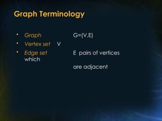
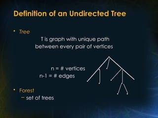
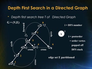
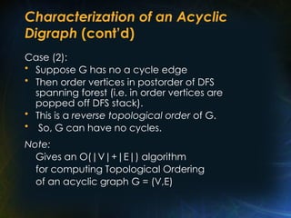
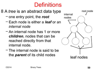
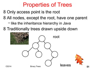
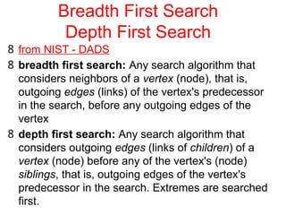
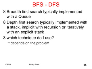
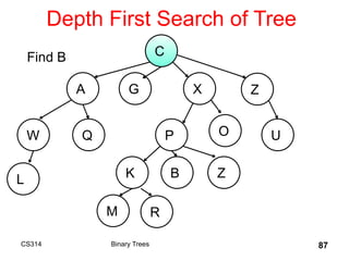
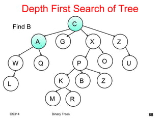
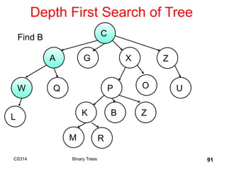
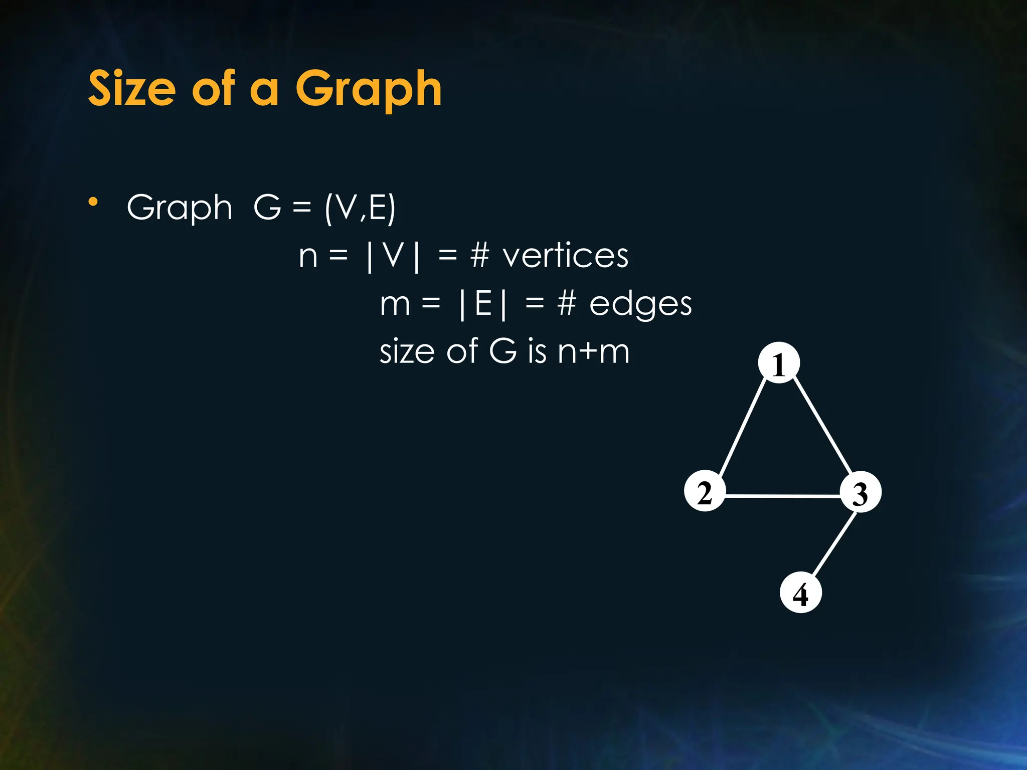
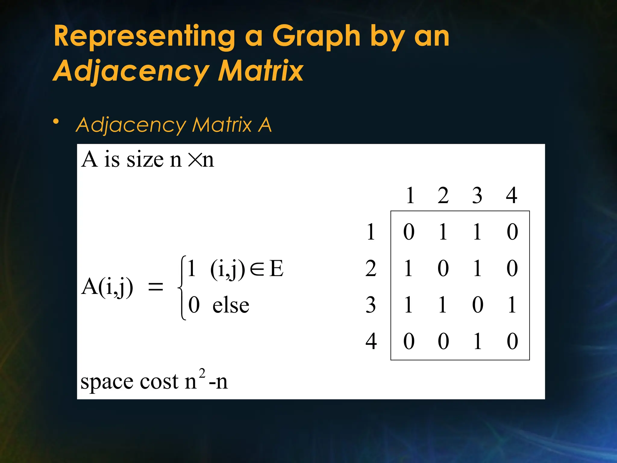
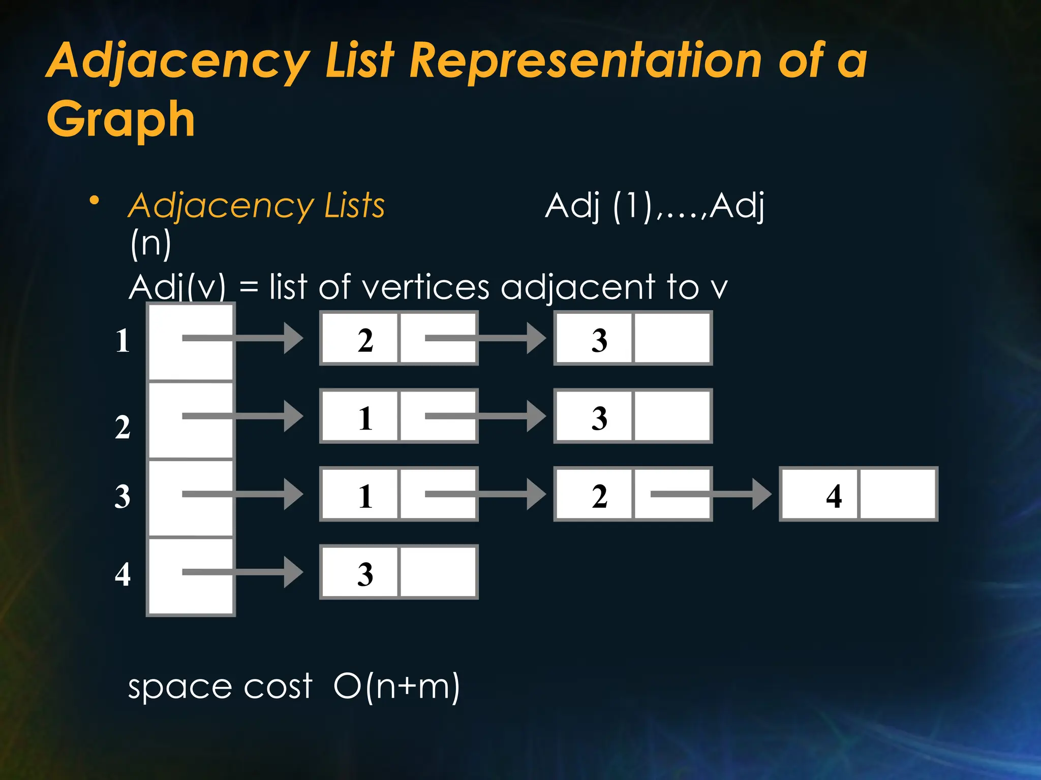
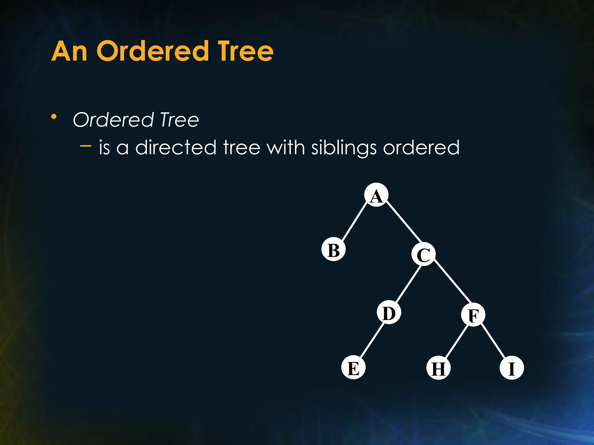
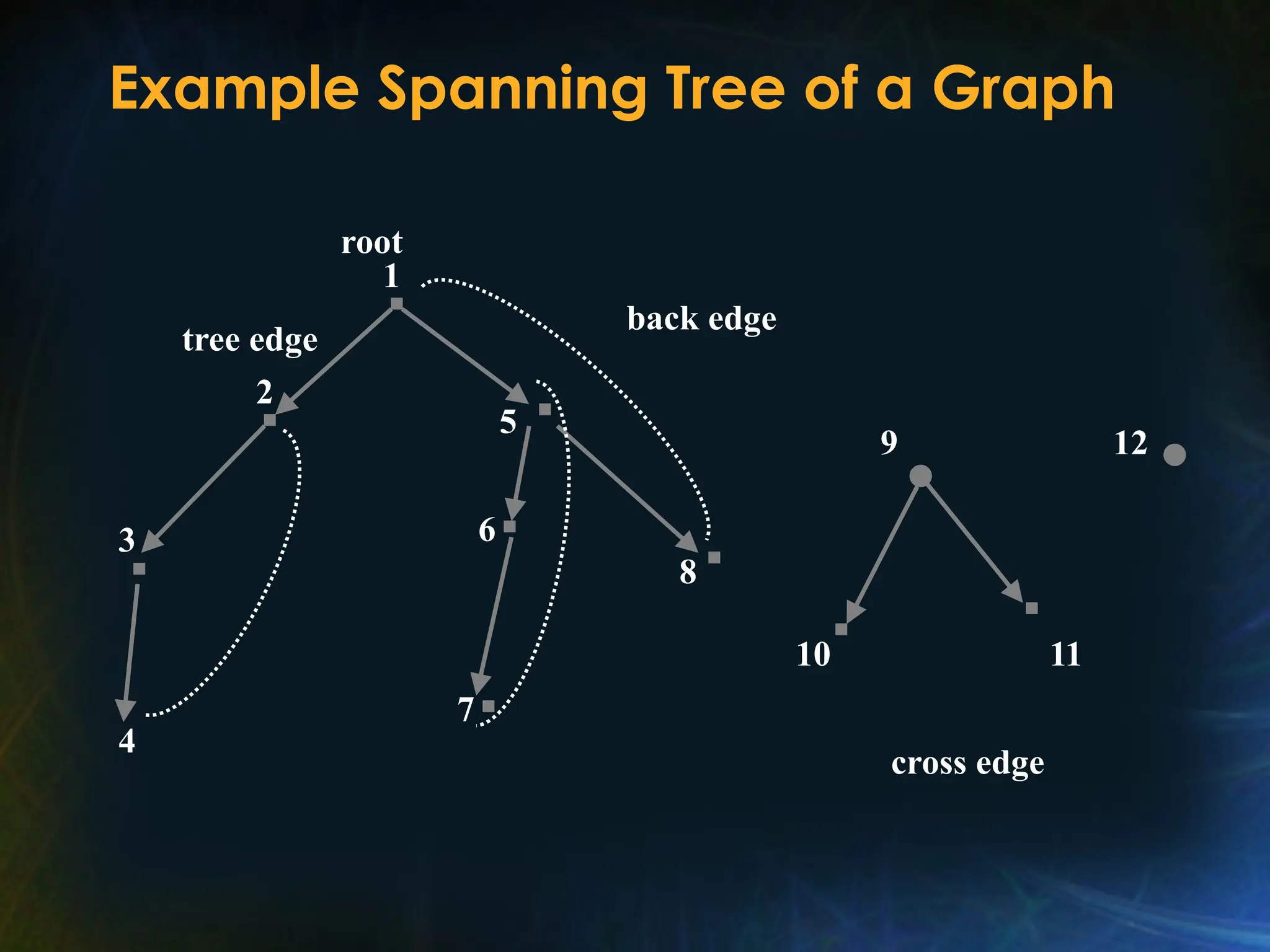
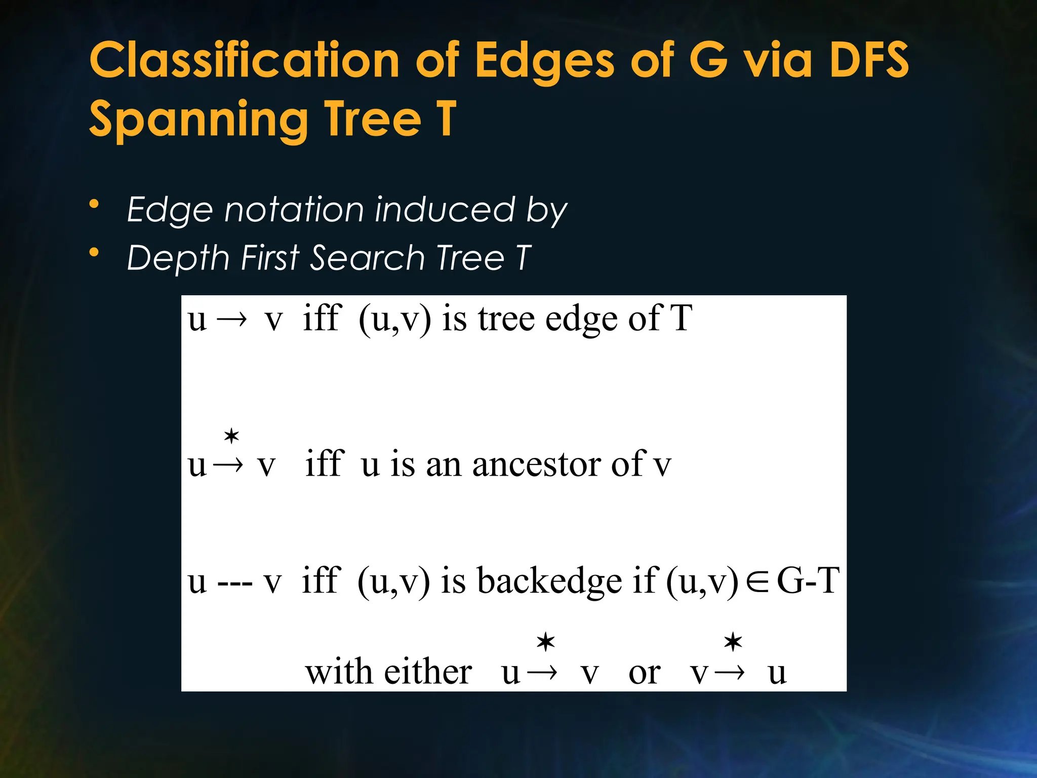
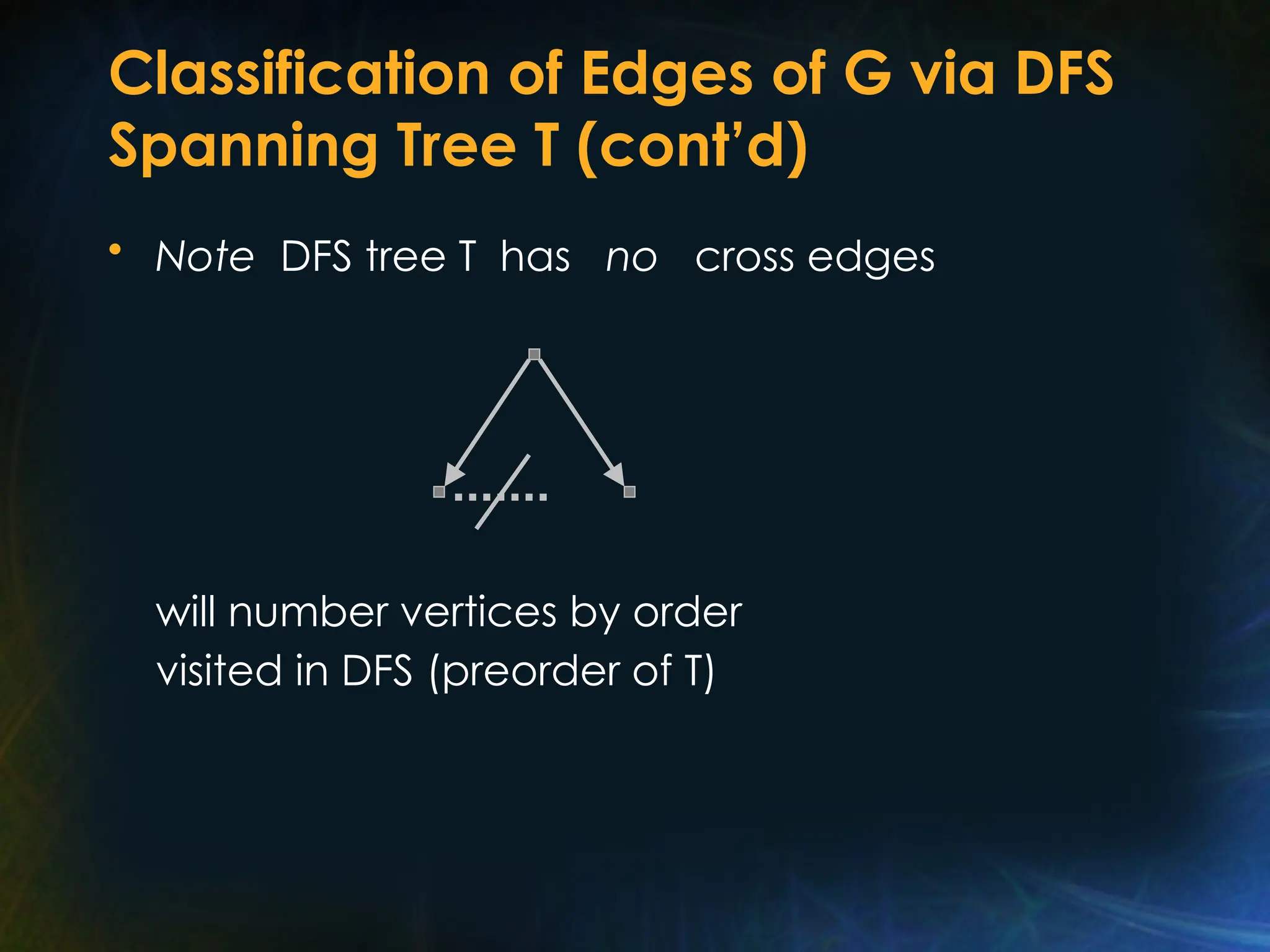
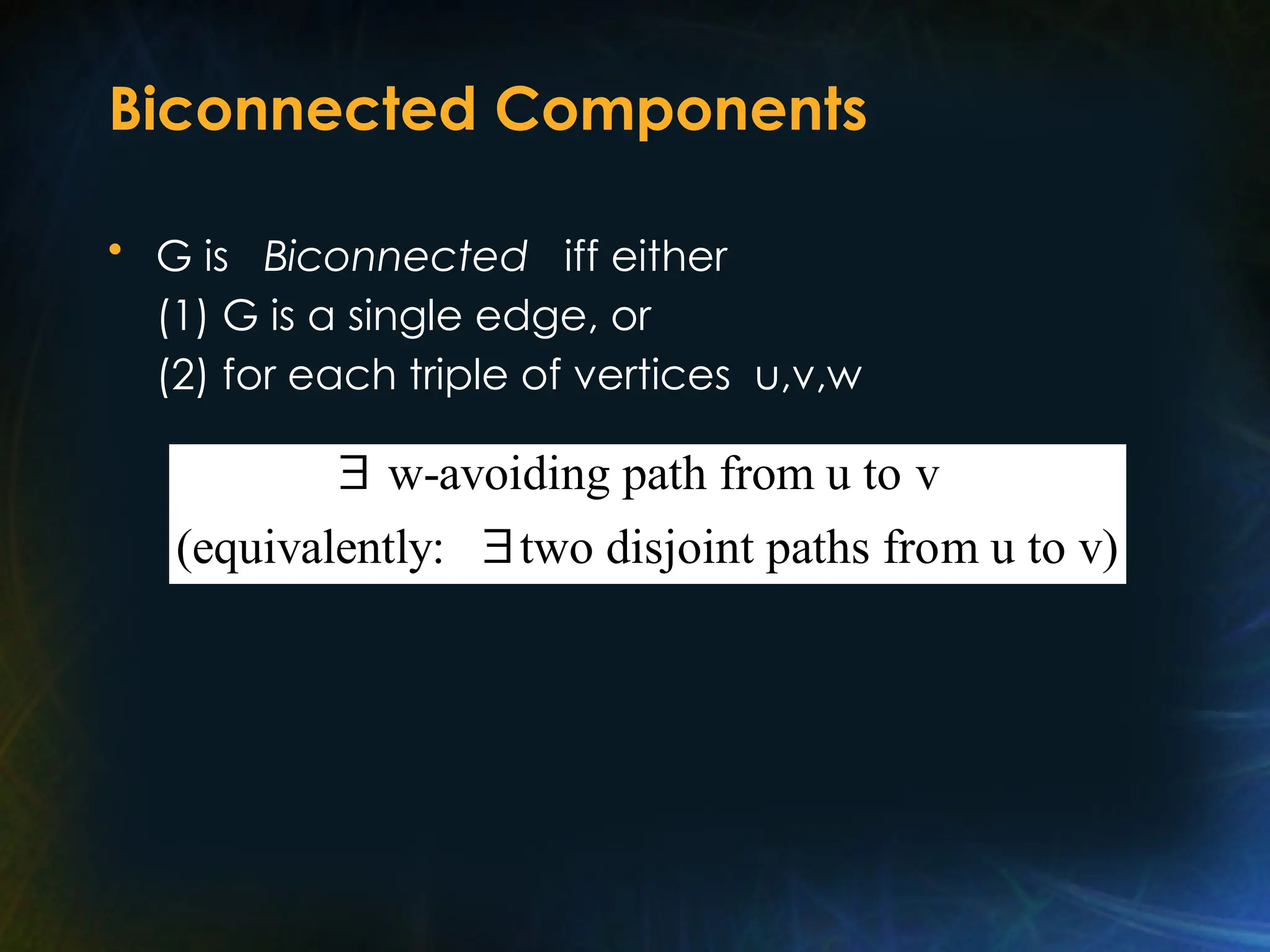
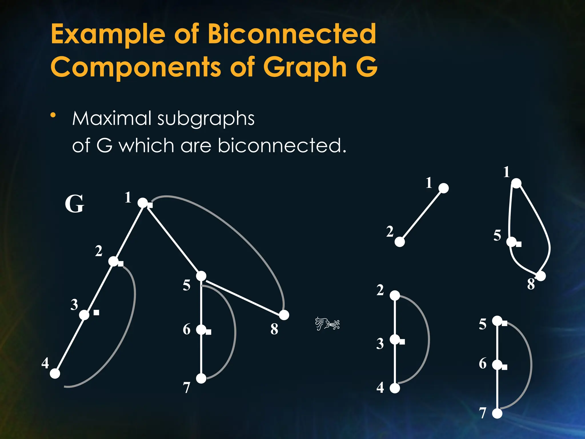
The document outlines various graph algorithms, particularly focusing on depth-first search (DFS), graph definitions, and spanning trees. It details concepts such as biconnected components, articulation points, and different representations of graphs, including adjacency matrices and lists. Additionally, it covers tree structures, including binary trees and their properties, along with traversal methods like preorder and postorder.


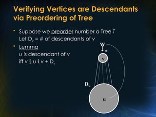
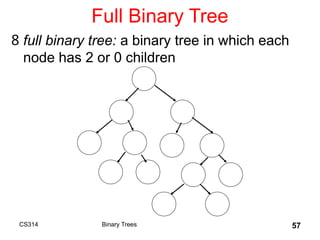
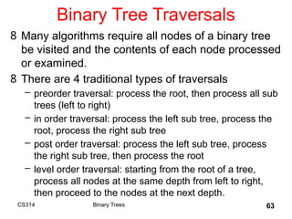
![Preorder Tree Traversal
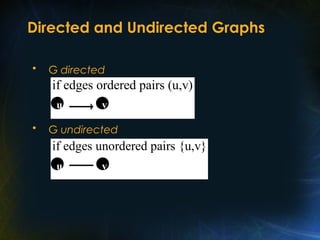
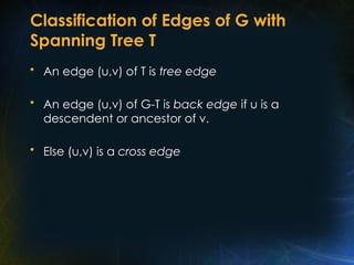
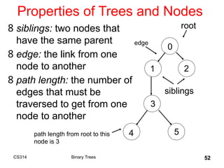
• Preorder A,B,C,D,E,F,H,I
[1] root (order vertices as pushed on
stack)
[2] preorder left subtree
[3] preorder right subtree
B
A
C
D
E
F
H I](https://image.slidesharecdn.com/unit4-partb-250122121219-e8a61200/85/Unit-4-PartB-of-data-design-and-algorithms-18-320.jpg)
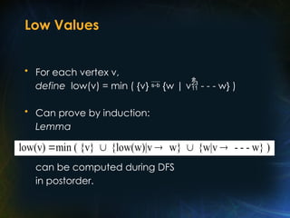
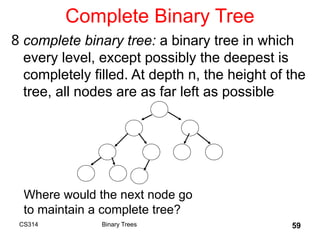
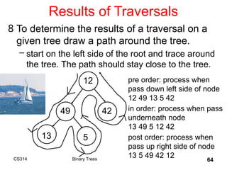
![Postorder Tree Traversal
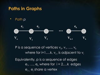
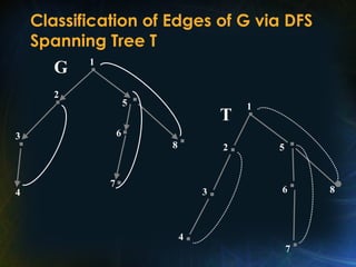
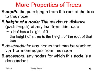
• Postorder B,E,D,H,I,F,C,A
[1] postorder left subtree
[2] postorder right subtree
[3] root (order vertices as popped off
stack)
B
A
C
D
E
F
H I](https://image.slidesharecdn.com/unit4-partb-250122121219-e8a61200/85/Unit-4-PartB-of-data-design-and-algorithms-19-320.jpg)
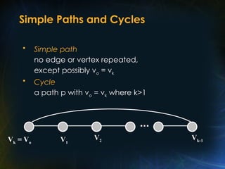
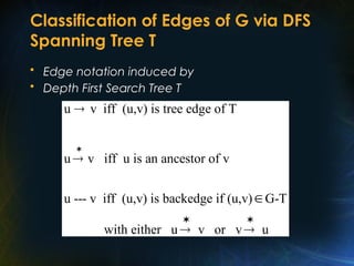
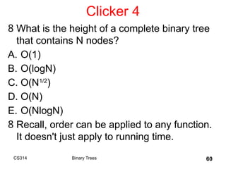
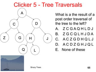
![Tarjan’s Depth First Search Algorithm
• We assume a RAM machine model
• Algorithm Depth First Search
graph G (V,E) represented by
adjacency lists Adj(v) for each v V
[0] N 0
[1] all v V (number (v) 0
children (v) ( ) )
[2] all v V do
Input
for do
od
for
number (v) 0 DFS(v)
[3] spanning forest defined by children
if then
output
](https://image.slidesharecdn.com/unit4-partb-250122121219-e8a61200/85/Unit-4-PartB-of-data-design-and-algorithms-23-320.jpg)
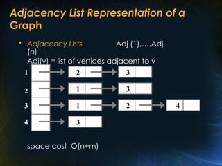
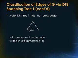
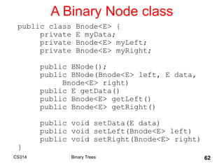
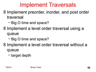
![Recursive DFS Procedure
DFS(v)
[1] N N + 1; number (v) N
[2] for each u Adj(v)
number (u) 0
(add u to children (v); DFS(u))
recursive procedure
do
if then
](https://image.slidesharecdn.com/unit4-partb-250122121219-e8a61200/85/Unit-4-PartB-of-data-design-and-algorithms-24-320.jpg)


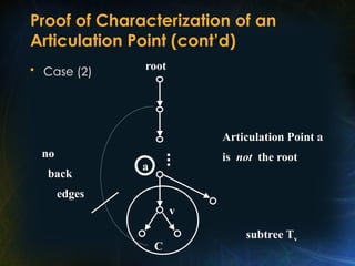
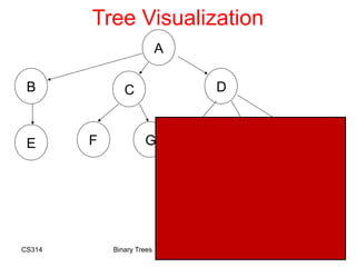
![Graph with DFS Numbering and Low
Values in Brackets
7[5]
1[1]
2[2]
4[2]
3[2]
5[1]
8[1]
6[5]
v[low(v)]
Number vertices
by DFS number](https://image.slidesharecdn.com/unit4-partb-250122121219-e8a61200/85/Unit-4-PartB-of-data-design-and-algorithms-32-320.jpg)


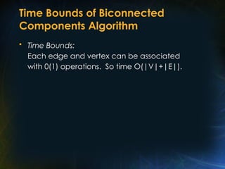
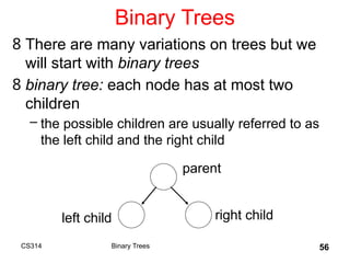
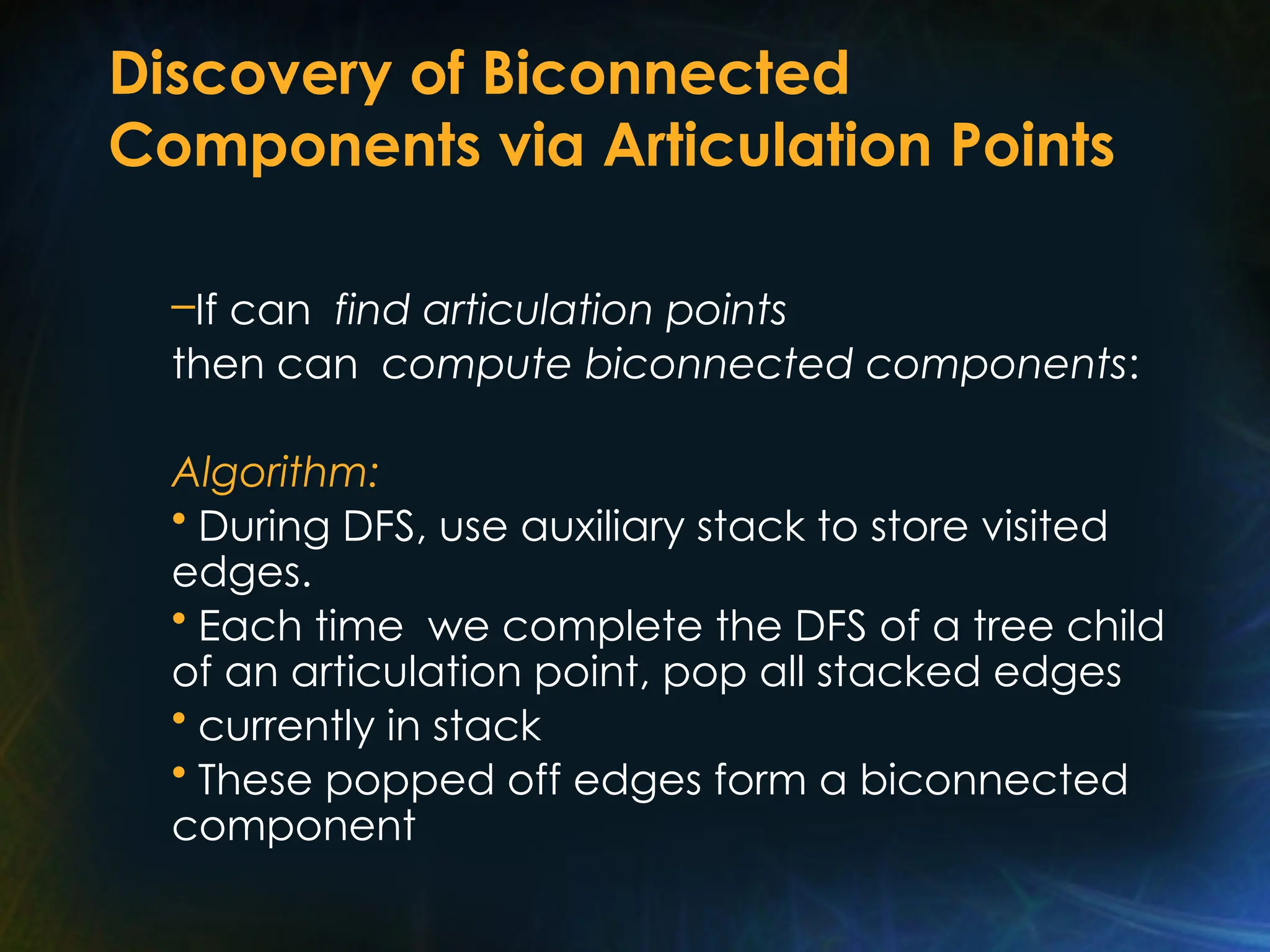
![Biconnected Components Algorithm
[0] initialize a STACK to empty
During a DFS traversal do
[1] add visited edge to STACK
[2] compute low of visited vertex v using Lemma
[3] test if v is an articulation point
[4] if so, for each u children (v) in order
where low (u) > v
do Pop all edges in STACK
upto and including tree edge (v,u)
Output popped edges as a
biconnected component of G
od](https://image.slidesharecdn.com/unit4-partb-250122121219-e8a61200/85/Unit-4-PartB-of-data-design-and-algorithms-42-320.jpg)


![Preorder Tree Traversal
• Preorder A,B,C,D,E,F,H,I
[1] root (order vertices as pushed on
stack)
[2] preorder left subtree
[3] preorder right subtree
B
A
C
D
E
F
H I](https://image.slidesharecdn.com/unit4-partb-250122121219-e8a61200/75/Unit-4-PartB-of-data-design-and-algorithms-18-2048.jpg)
![Postorder Tree Traversal
• Postorder B,E,D,H,I,F,C,A
[1] postorder left subtree
[2] postorder right subtree
[3] root (order vertices as popped off
stack)
B
A
C
D
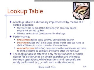
E
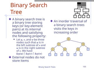
F
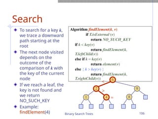
H I](https://image.slidesharecdn.com/unit4-partb-250122121219-e8a61200/75/Unit-4-PartB-of-data-design-and-algorithms-19-2048.jpg)


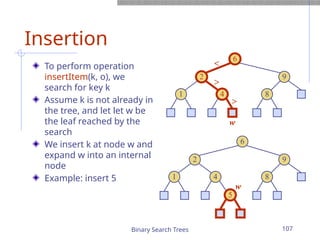
![Tarjan’s Depth First Search Algorithm
• We assume a RAM machine model
• Algorithm Depth First Search
graph G (V,E) represented by
adjacency lists Adj(v) for each v V
[0] N 0
[1] all v V (number (v) 0
children (v) ( ) )
[2] all v V do
Input
for do
od
for
number (v) 0 DFS(v)
[3] spanning forest defined by children
if then
output
](https://image.slidesharecdn.com/unit4-partb-250122121219-e8a61200/75/Unit-4-PartB-of-data-design-and-algorithms-23-2048.jpg)
![Recursive DFS Procedure
DFS(v)
[1] N N + 1; number (v) N
[2] for each u Adj(v)
number (u) 0
(add u to children (v); DFS(u))
recursive procedure
do
if then
](https://image.slidesharecdn.com/unit4-partb-250122121219-e8a61200/75/Unit-4-PartB-of-data-design-and-algorithms-24-2048.jpg)


![Graph with DFS Numbering and Low
Values in Brackets
7[5]
1[1]
2[2]
4[2]
3[2]
5[1]
8[1]
6[5]
v[low(v)]
Number vertices
by DFS number](https://image.slidesharecdn.com/unit4-partb-250122121219-e8a61200/75/Unit-4-PartB-of-data-design-and-algorithms-32-2048.jpg)


![Biconnected Components Algorithm
[0] initialize a STACK to empty
During a DFS traversal do
[1] add visited edge to STACK
[2] compute low of visited vertex v using Lemma
[3] test if v is an articulation point
[4] if so, for each u children (v) in order
where low (u) > v
do Pop all edges in STACK
upto and including tree edge (v,u)
Output popped edges as a
biconnected component of G
od](https://image.slidesharecdn.com/unit4-partb-250122121219-e8a61200/75/Unit-4-PartB-of-data-design-and-algorithms-42-2048.jpg)