Unit i basic concepts of algorithms

UNIT I
BASIC CONCEPTS OF
ALGORITHMS

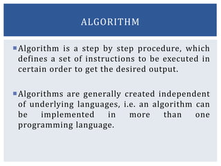
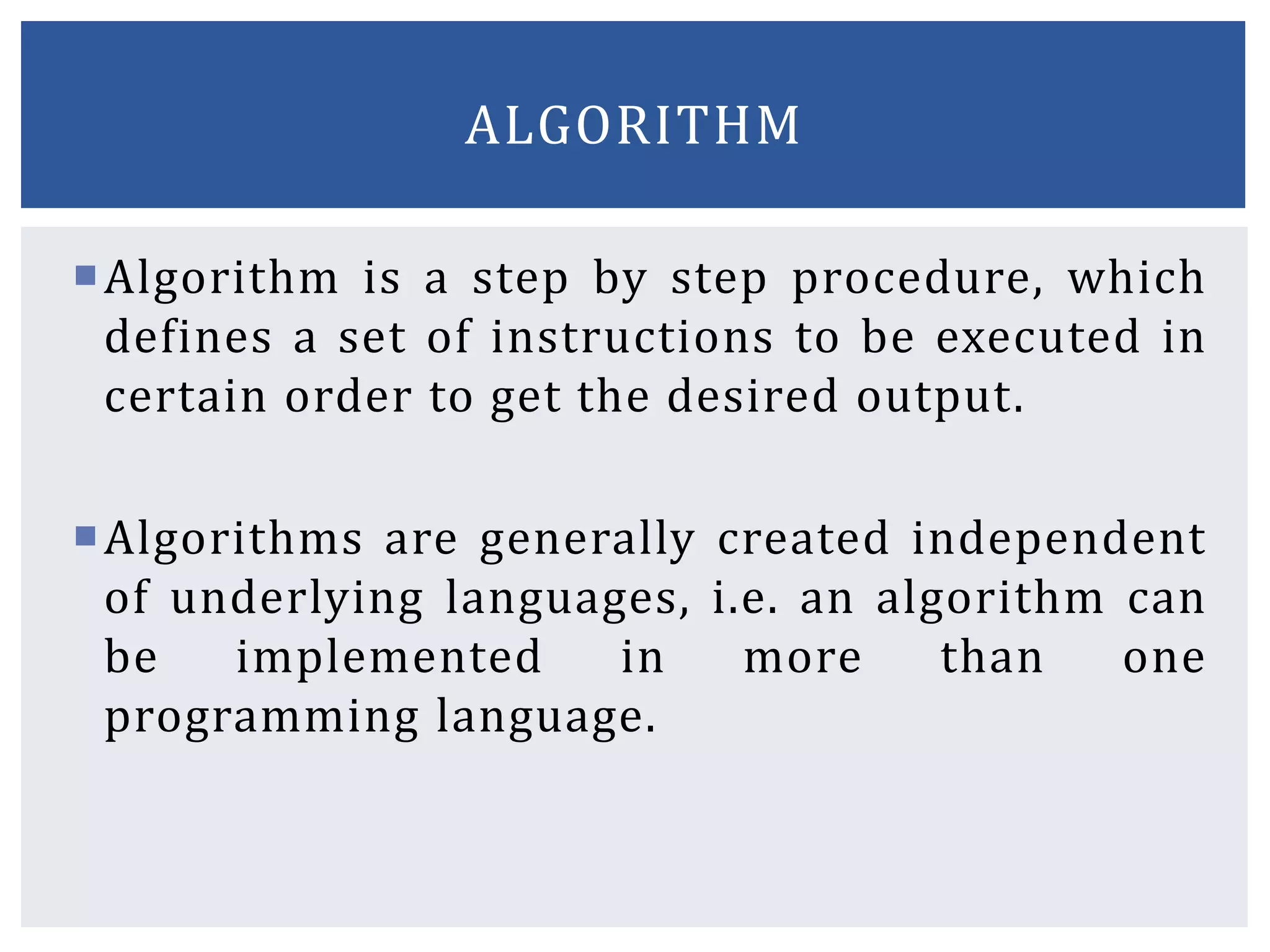
Algorithm is a step by step procedure, which
defines a set of instructions to be executed in
certain order to get the desired output.
Algorithms are generally created independent
of underlying languages, i.e. an algorithm can
be implemented in more than one
programming language.
ALGORITHM

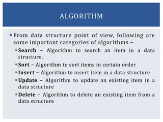
From data structure point of view, following are
some important categories of algorithms −
Search − Algorithm to search an item in a data
structure.
Sort − Algorithm to sort items in certain order
Insert − Algorithm to insert item in a data structure
Update − Algorithm to update an existing item in a
data structure
Delete − Algorithm to delete an existing item from a
data structure
ALGORITHM

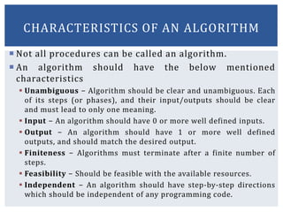
 Not all procedures can be called an algorithm.
 An algorithm should have the below mentioned
characteristics
 Unambiguous − Algorithm should be clear and unambiguous. Each
of its steps (or phases), and their input/outputs should be clear
and must lead to only one meaning.
 Input − An algorithm should have 0 or more well defined inputs.
 Output − An algorithm should have 1 or more well defined
outputs, and should match the desired output.
 Finiteness − Algorithms must terminate after a finite number of
steps.
 Feasibility − Should be feasible with the available resources.
 Independent − An algorithm should have step-by-step directions
which should be independent of any programming code.
CHARACTERISTICS OF AN ALGORITHM

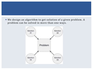
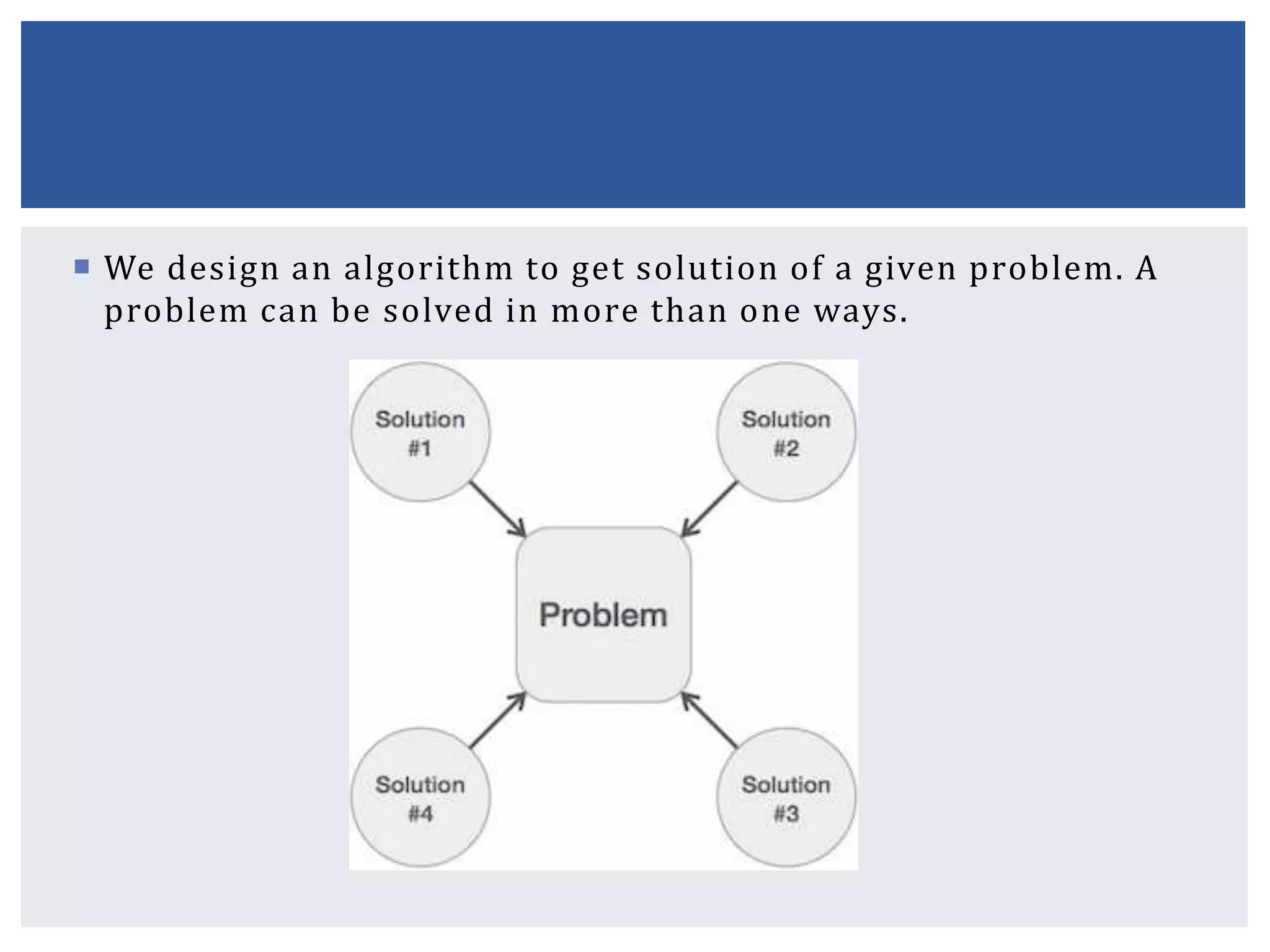
 We design an algorithm to get solution of a given problem. A
problem can be solved in more than one ways.

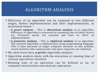
 Efficiency of an algorithm can be analyzed at two different
stages, before implementation and after implementation, as
mentioned below −
 A priori analysis − This is theoretical analysis of an algorithm.
Efficiency of algorithm is measured by assuming that all other factors
e.g. Processor speed, are constant and have no effect on
implementation.
 A posterior analysis − This is empirical analysis of an algorithm.
The selected algorithm is implemented using programming language.
This is then executed on target computer machine. In this analysis,
actual statistics like running time and space required, are collected.
 We shall learn here a priori algorithm analysis.
 Algorithm analysis deals with the execution or running time of
various operations involved.
 Running time of an operation can be defined as no. of
computer instructions executed per operation.
ALGORITHM ANALYSIS

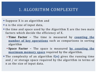
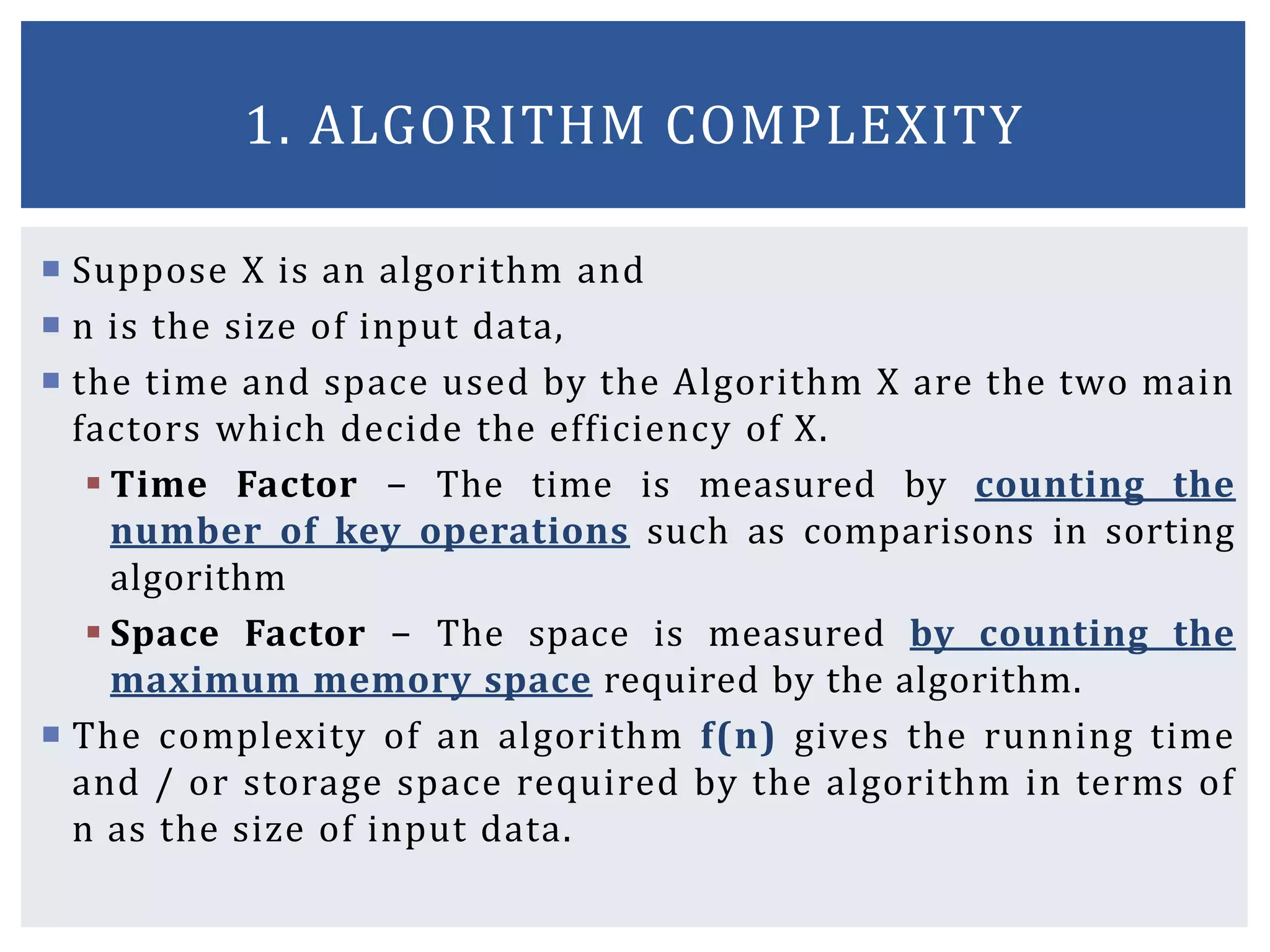
 Suppose X is an algorithm and
 n is the size of input data,
 the time and space used by the Algorithm X are the two main
factors which decide the efficiency of X.
 Time Factor − The time is measured by counting the
number of key operations such as comparisons in sorting
algorithm
 Space Factor − The space is measured by counting the
maximum memory space required by the algorithm.
 The complexity of an algorithm f(n) gives the running time
and / or storage space required by the algorithm in terms of
n as the size of input data.
1. ALGORITHM COMPLEXITY

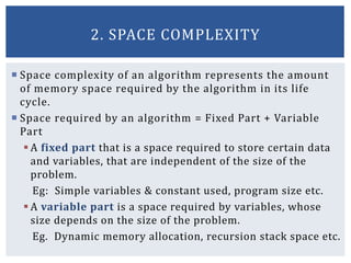
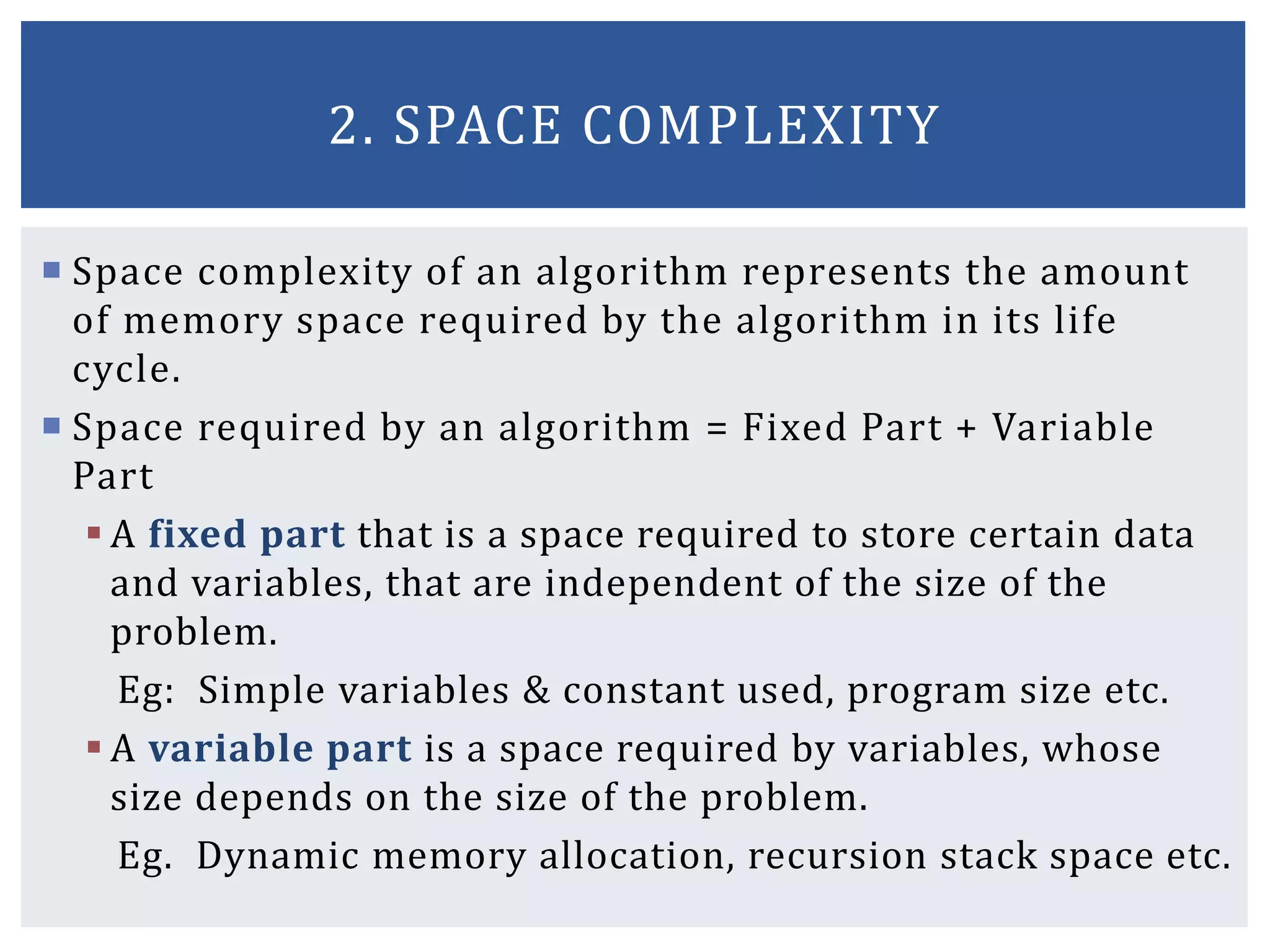
 Space complexity of an algorithm represents the amount
of memory space required by the algorithm in its life
cycle.
 Space required by an algorithm = Fixed Part + Variable
Part
 A fixed part that is a space required to store certain data
and variables, that are independent of the size of the
problem.
Eg: Simple variables & constant used, program size etc.
 A variable part is a space required by variables, whose
size depends on the size of the problem.
Eg. Dynamic memory allocation, recursion stack space etc.
2. SPACE COMPLEXITY

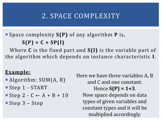
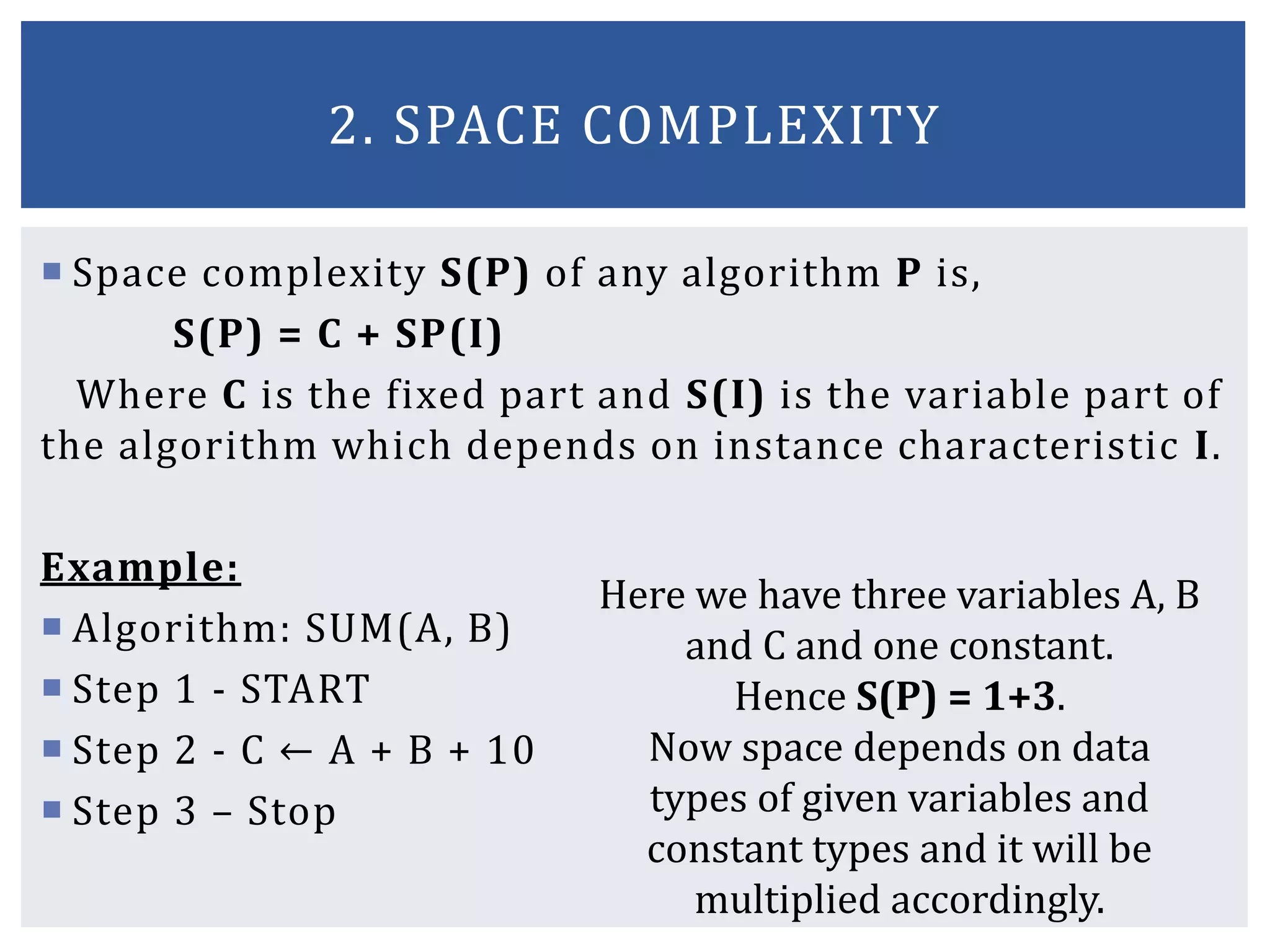
 Space complexity S(P) of any algorithm P is,
S(P) = C + SP(I)
Where C is the fixed part and S(I) is the variable part of
the algorithm which depends on instance characteristic I.
Example:
 Algorithm: SUM(A, B)
 Step 1 - START
 Step 2 - C ← A + B + 10
 Step 3 – Stop
2. SPACE COMPLEXITY
Here we have three variables A, B
and C and one constant.
Hence S(P) = 1+3.
Now space depends on data
types of given variables and
constant types and it will be
multiplied accordingly.

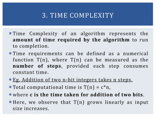
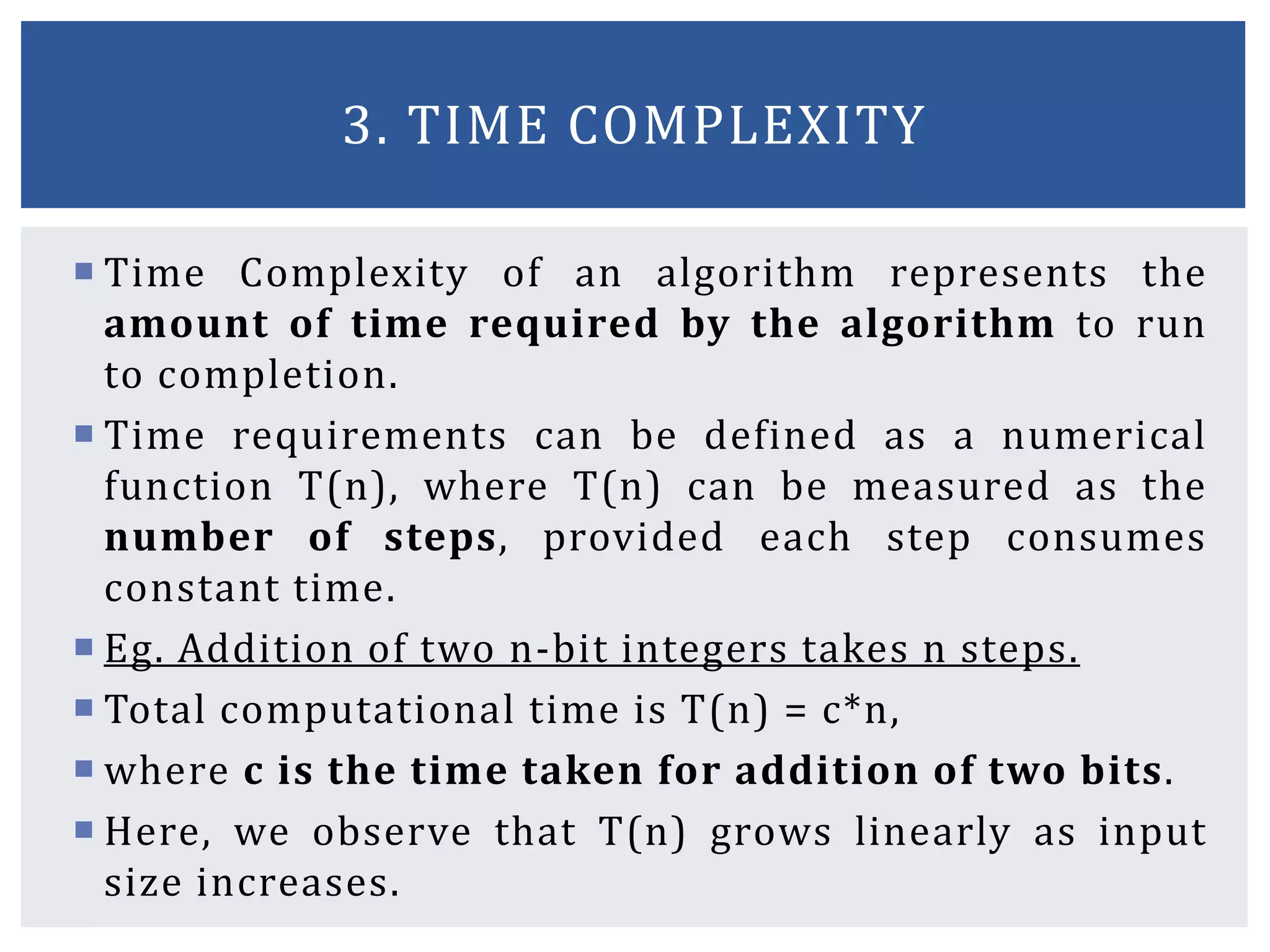
 Time Complexity of an algorithm represents the
amount of time required by the algorithm to run
to completion.
 Time requirements can be defined as a numerical
function T(n), where T(n) can be measured as the
number of steps, provided each step consumes
constant time.
 Eg. Addition of two n-bit integers takes n steps.
 Total computational time is T(n) = c*n,
 where c is the time taken for addition of two bits.
 Here, we observe that T(n) grows linearly as input
size increases.
3. TIME COMPLEXITY

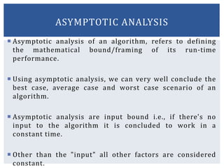
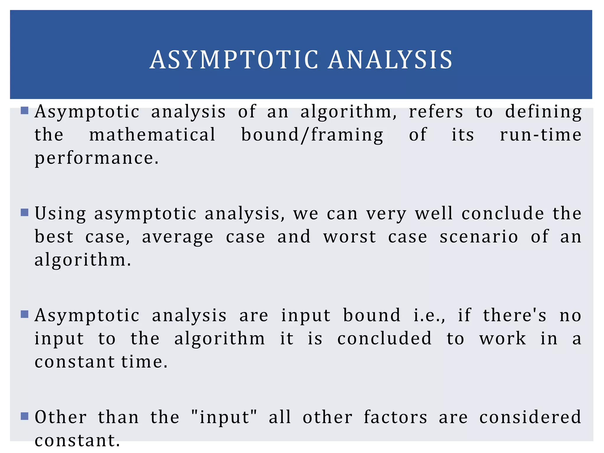
 Asymptotic analysis of an algorithm, refers to defining
the mathematical bound/framing of its run-time
performance.
 Using asymptotic analysis, we can very well conclude the
best case, average case and worst case scenario of an
algorithm.
 Asymptotic analysis are input bound i.e., if there's no
input to the algorithm it is concluded to work in a
constant time.
 Other than the "input" all other factors are considered
constant.
ASYMPTOTIC ANALYSIS

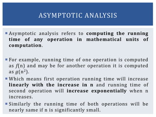
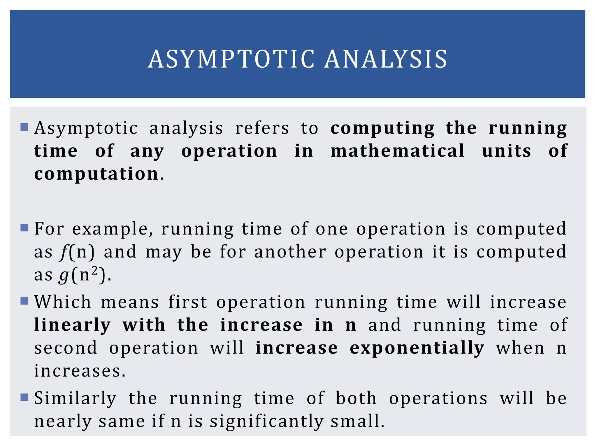
 Asymptotic analysis refers to computing the running
time of any operation in mathematical units of
computation.
 For example, running time of one operation is computed
as f(n) and may be for another operation it is computed
as g(n2).
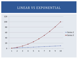
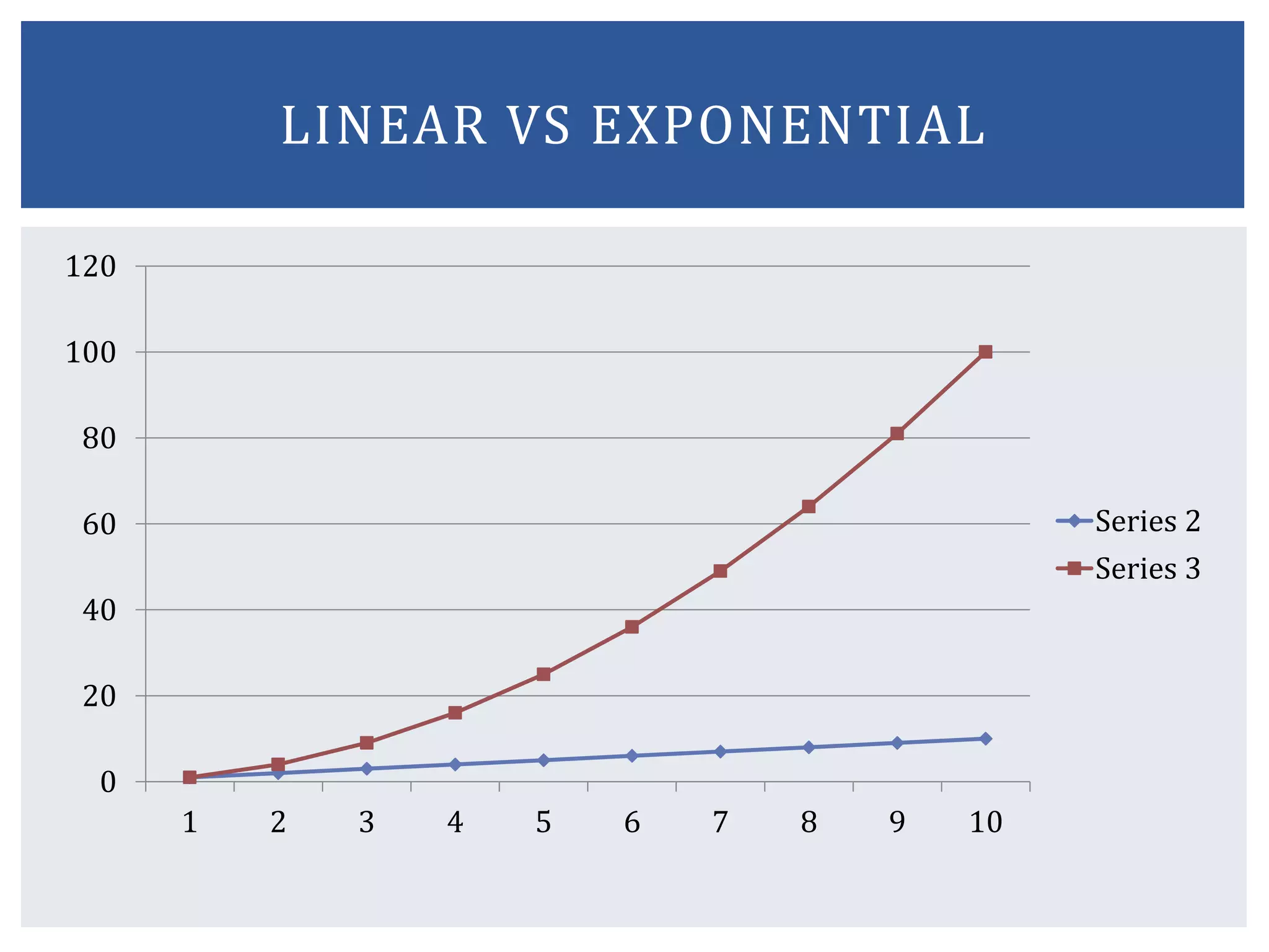
 Which means first operation running time will increase
linearly with the increase in n and running time of
second operation will increase exponentially when n
increases.
 Similarly the running time of both operations will be
nearly same if n is significantly small.
ASYMPTOTIC ANALYSIS

0
20
40
60
80
100
120
1 2 3 4 5 6 7 8 9 10
Series 2
Series 3
LINEAR VS EXPONENTIAL

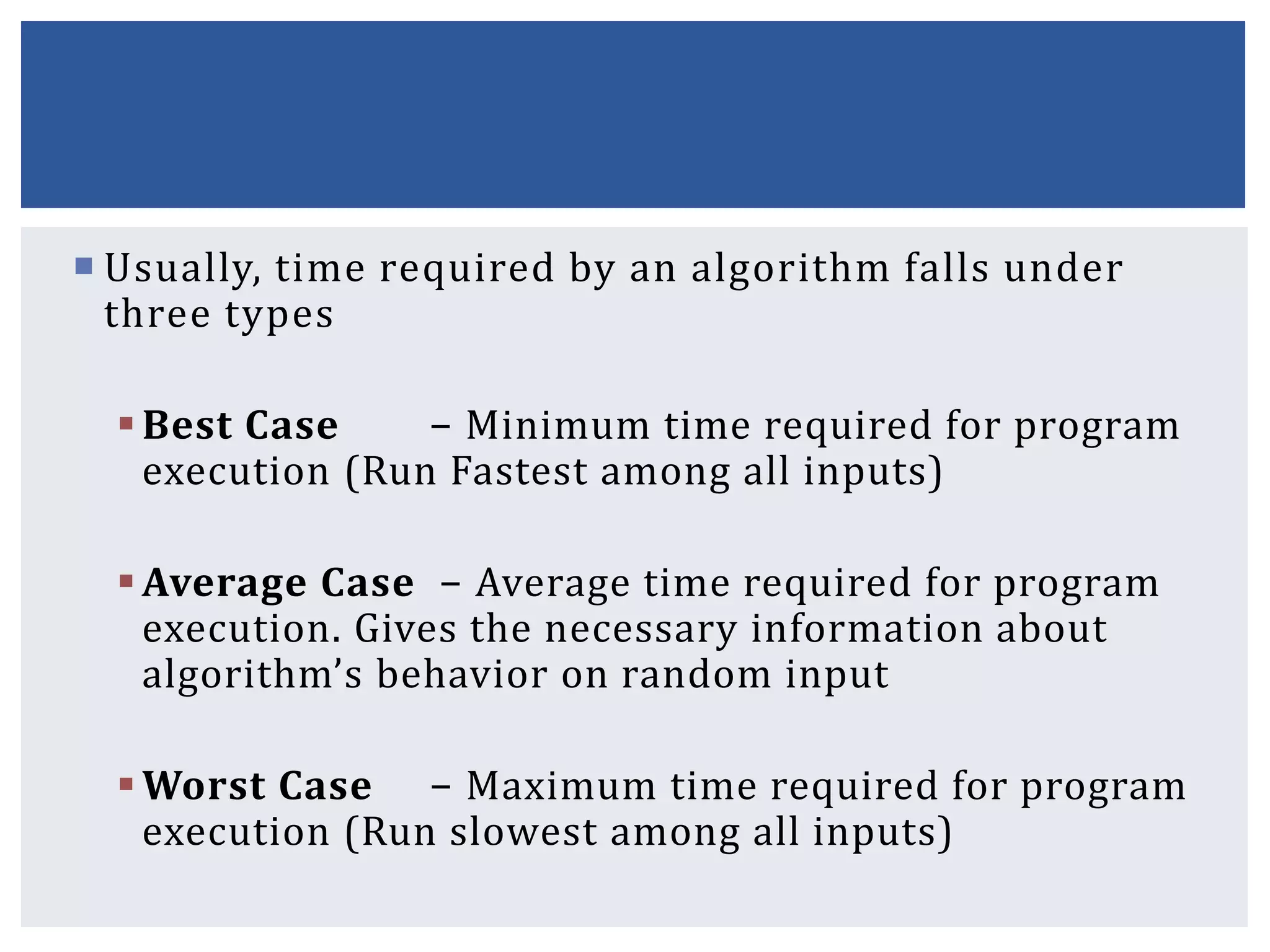
 Usually, time required by an algorithm falls under
three types
Best Case − Minimum time required for program
execution (Run Fastest among all inputs)
Average Case − Average time required for program
execution. Gives the necessary information about
algorithm’s behavior on random input
Worst Case − Maximum time required for program
execution (Run slowest among all inputs)

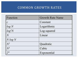
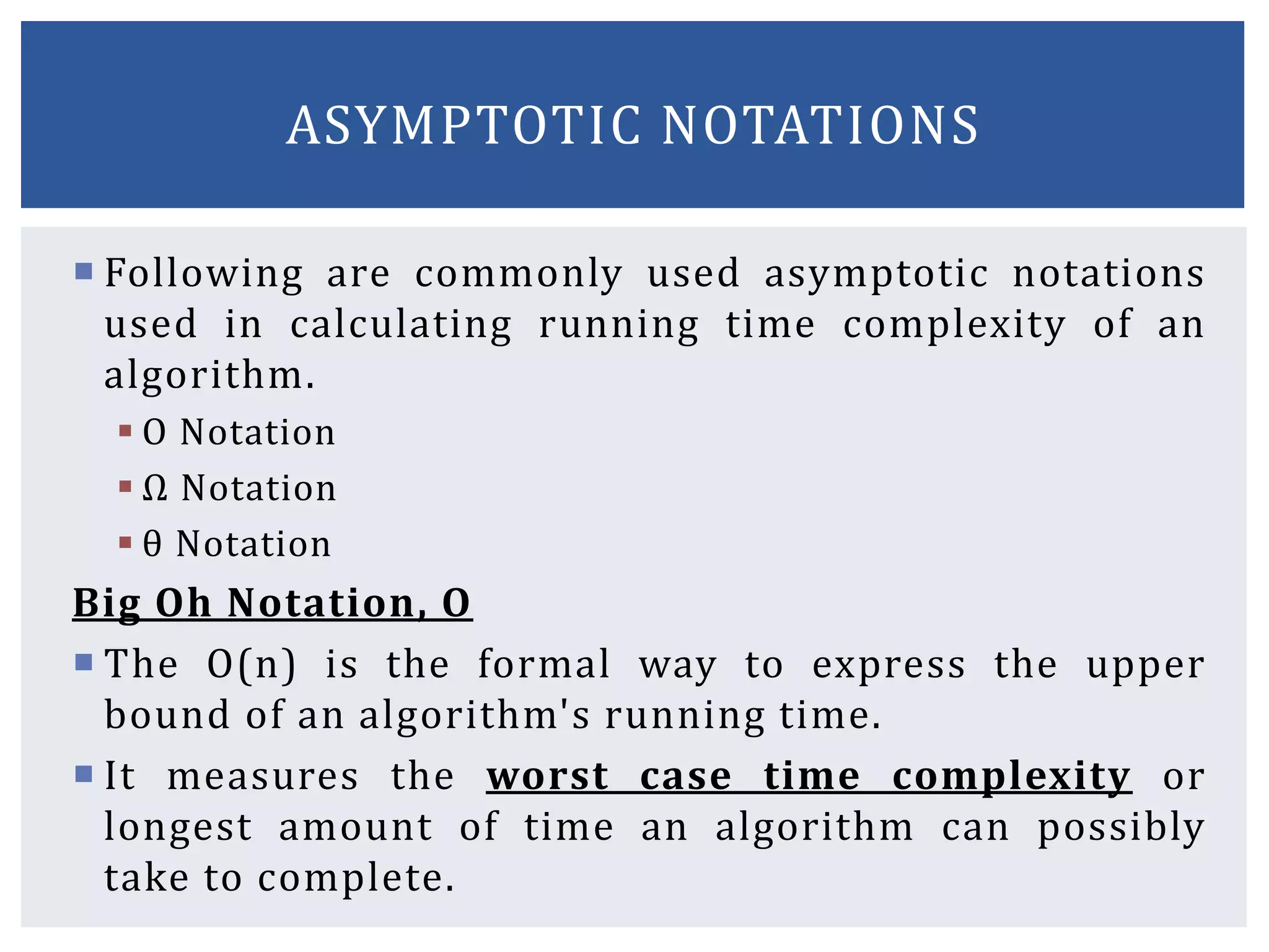
 Following are commonly used asymptotic notations
used in calculating running time complexity of an
algorithm.
 Ο Notation
 Ω Notation
 θ Notation
Big Oh Notation, Ο
 The Ο(n) is the formal way to express the upper
bound of an algorithm's running time.
 It measures the worst case time complexity or
longest amount of time an algorithm can possibly
take to complete.
ASYMPTOTIC NOTATIONS

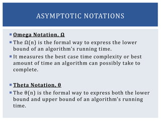
 Omega Notation, Ω
 The Ω(n) is the formal way to express the lower
bound of an algorithm's running time.
 It measures the best case time complexity or best
amount of time an algorithm can possibly take to
complete.
 Theta Notation, θ
 The θ(n) is the formal way to express both the lower
bound and upper bound of an algorithm's running
time.
ASYMPTOTIC NOTATIONS

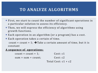
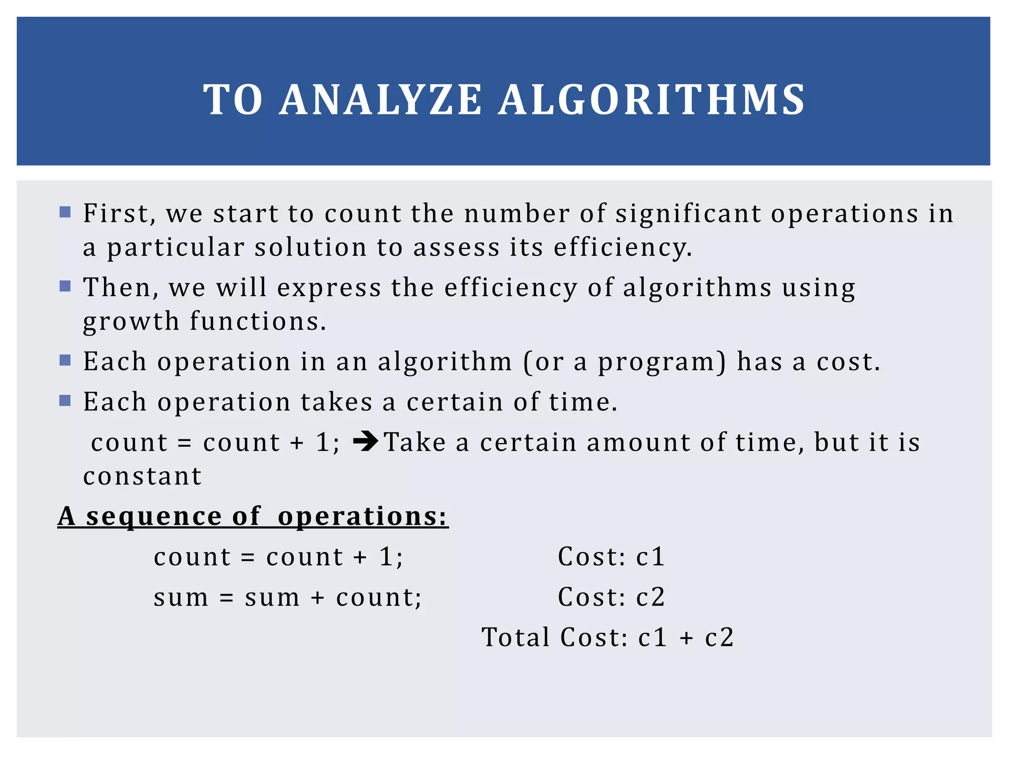
 First, we start to count the number of significant operations in
a particular solution to assess its efficiency.
 Then, we will express the efficiency of algorithms using
growth functions.
 Each operation in an algorithm (or a program) has a cost.
 Each operation takes a certain of time.
count = count + 1; Take a certain amount of time, but it is
constant
A sequence of operations:
count = count + 1; Cost: c1
sum = sum + count; Cost: c2
Total Cost: c1 + c2
TO ANALYZE ALGORITHMS

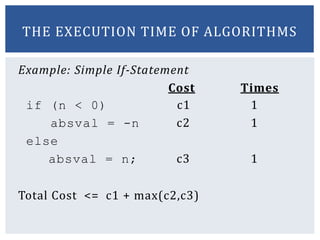
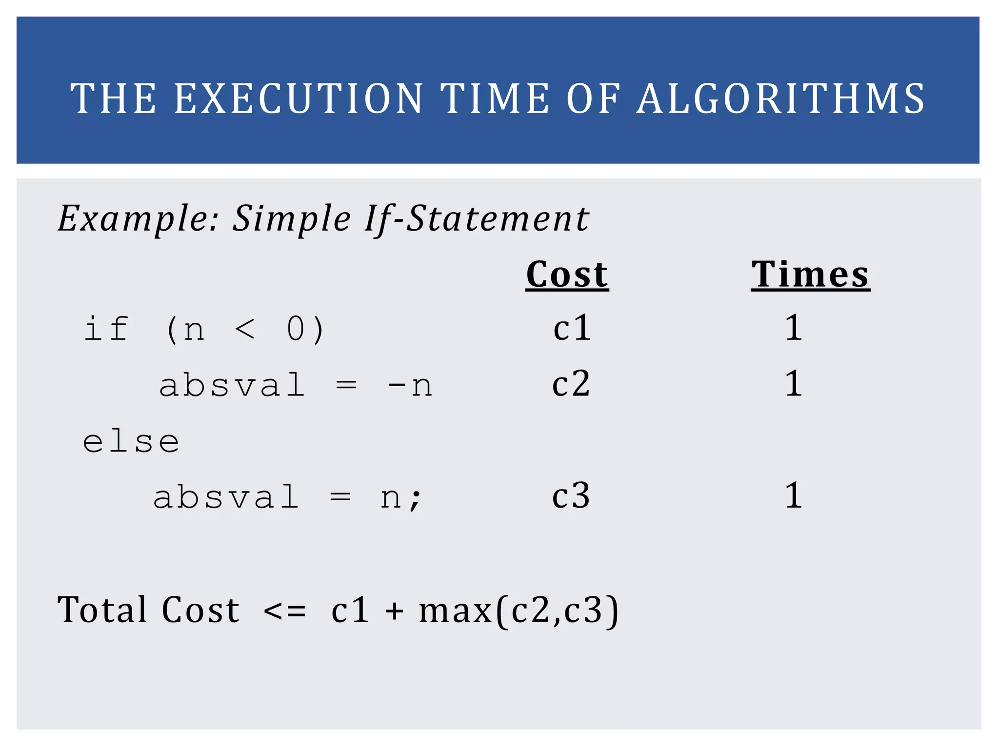
Example: Simple If-Statement
Cost Times
if (n < 0) c1 1
absval = -n c2 1
else
absval = n; c3 1
Total Cost <= c1 + max(c2,c3)
THE EXECUTION TIME OF ALGORITHMS

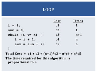
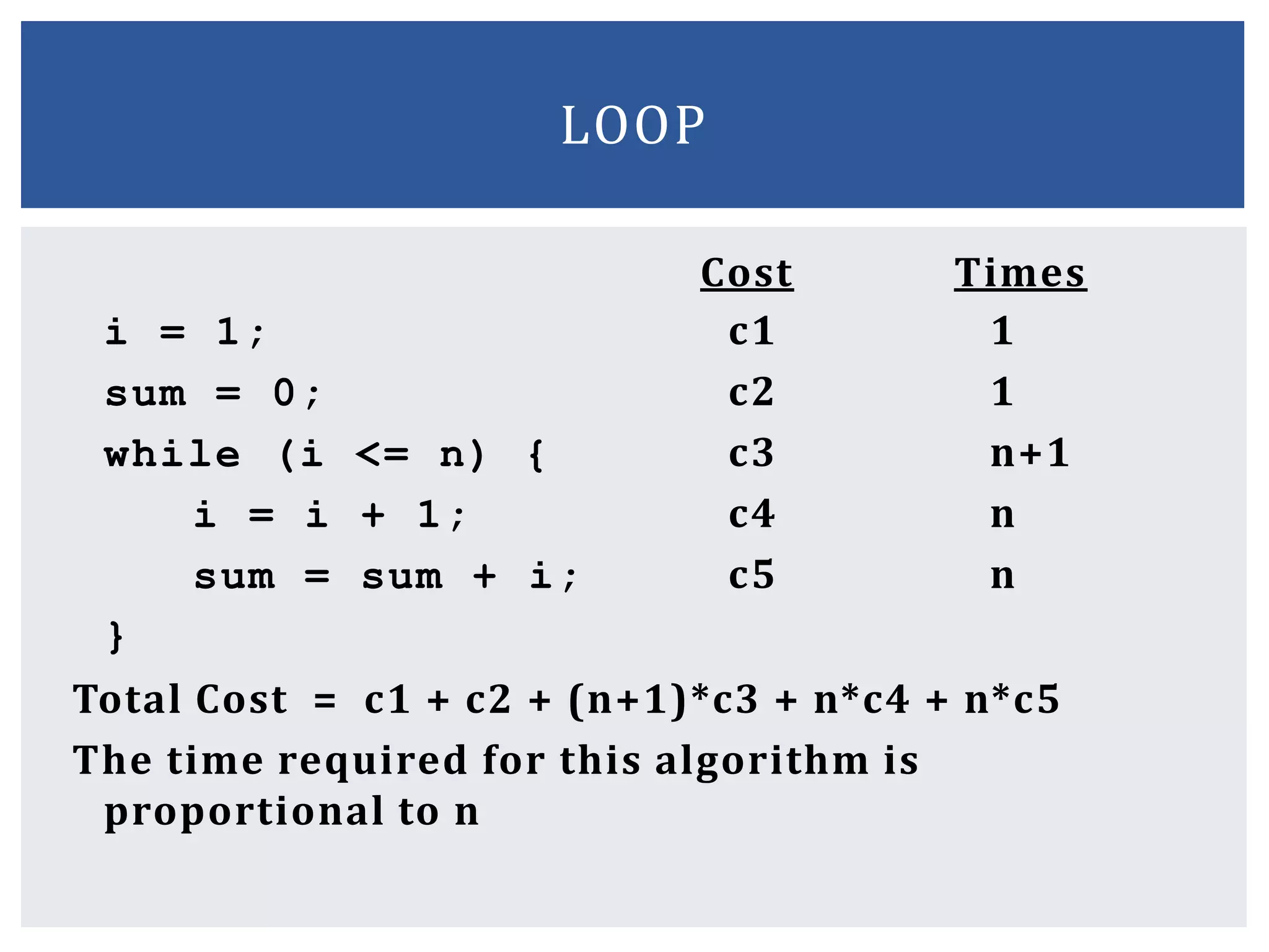
Cost Times
i = 1; c1 1
sum = 0; c2 1
while (i <= n) { c3 n+1
i = i + 1; c4 n
sum = sum + i; c5 n
}
Total Cost = c1 + c2 + (n+1)*c3 + n*c4 + n*c5
The time required for this algorithm is
proportional to n
LOOP

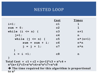
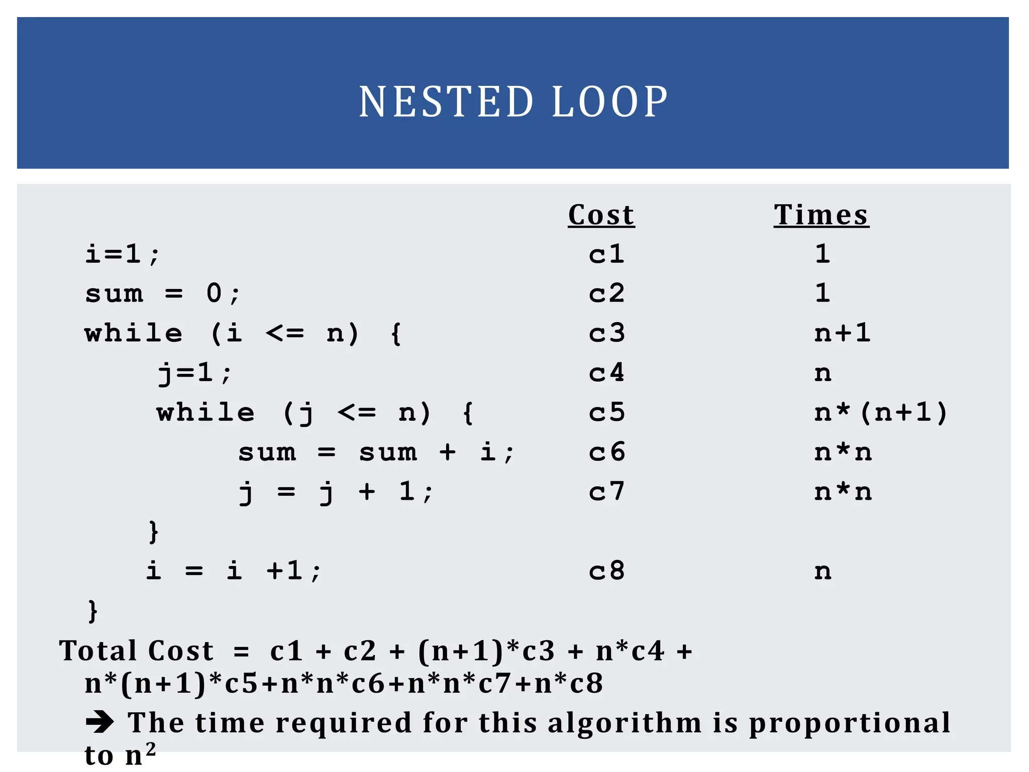
Cost Times
i=1; c1 1
sum = 0; c2 1
while (i <= n) { c3 n+1
j=1; c4 n
while (j <= n) { c5 n*(n+1)
sum = sum + i; c6 n*n
j = j + 1; c7 n*n
}
i = i +1; c8 n
}
Total Cost = c1 + c2 + (n+1)*c3 + n*c4 +
n*(n+1)*c5+n*n*c6+n*n*c7+n*c8
 The time required for this algorithm is proportional
to n2
NESTED LOOP

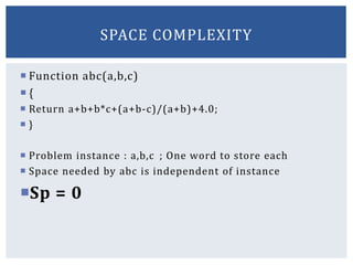
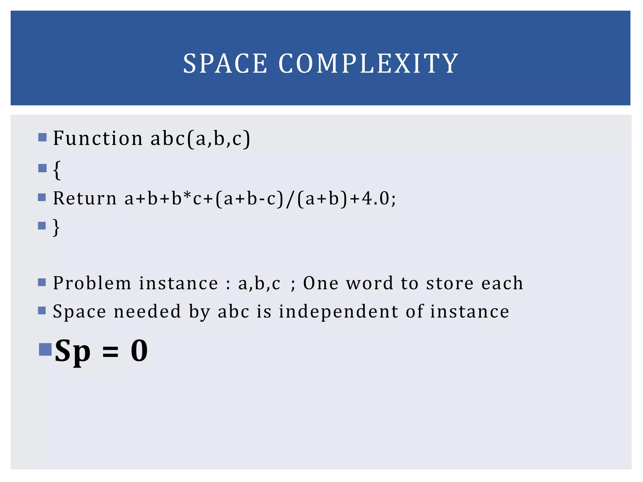
 Function abc(a,b,c)
 {
 Return a+b+b*c+(a+b-c)/(a+b)+4.0;
 }
 Problem instance : a,b,c ; One word to store each
 Space needed by abc is independent of instance
Sp = 0
SPACE COMPLEXITY

 Function Sum(a,n) {
 S:=0.0;
 For i:=1 to n do
 S:= s+a[i];
 Return S;
 }
 Characterized by n
 Space needed by a[n], n, i, S
Ssum(n) >= (n+3)
LOOP

Algorithm Rsum(a,n) {
If(n<=0) then return 0.0;
Else return Rsum(a,n-1)+a[n]; }
 Instances are characterized by n
 Stack Space: Formal parameter + Local variables +
Return Address
 Variables : a, n, and return address (3)
 Depth of recursion: n+1
SRSum(n) >= 3(n+1)
RECURSION

CENG 213 Data Structures 24
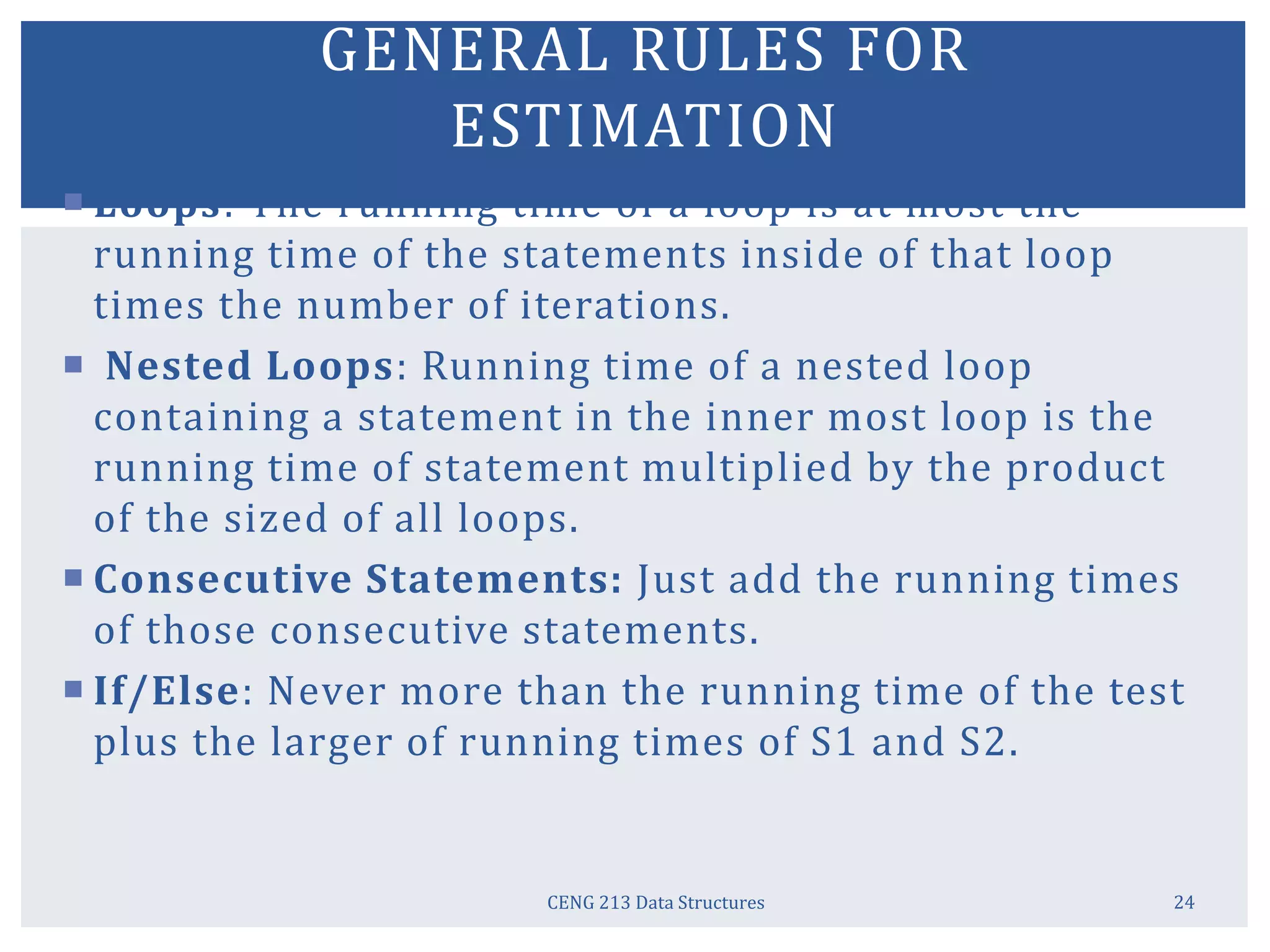
GENERAL RULES FOR
ESTIMATION
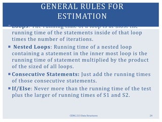
 Loops: The running time of a loop is at most the
running time of the statements inside of that loop
times the number of iterations.
 Nested Loops: Running time of a nested loop
containing a statement in the inner most loop is the
running time of statement multiplied by the product
of the sized of all loops.
 Consecutive Statements: Just add the running times
of those consecutive statements.
 If/Else: Never more than the running time of the test
plus the larger of running times of S1 and S2.

25
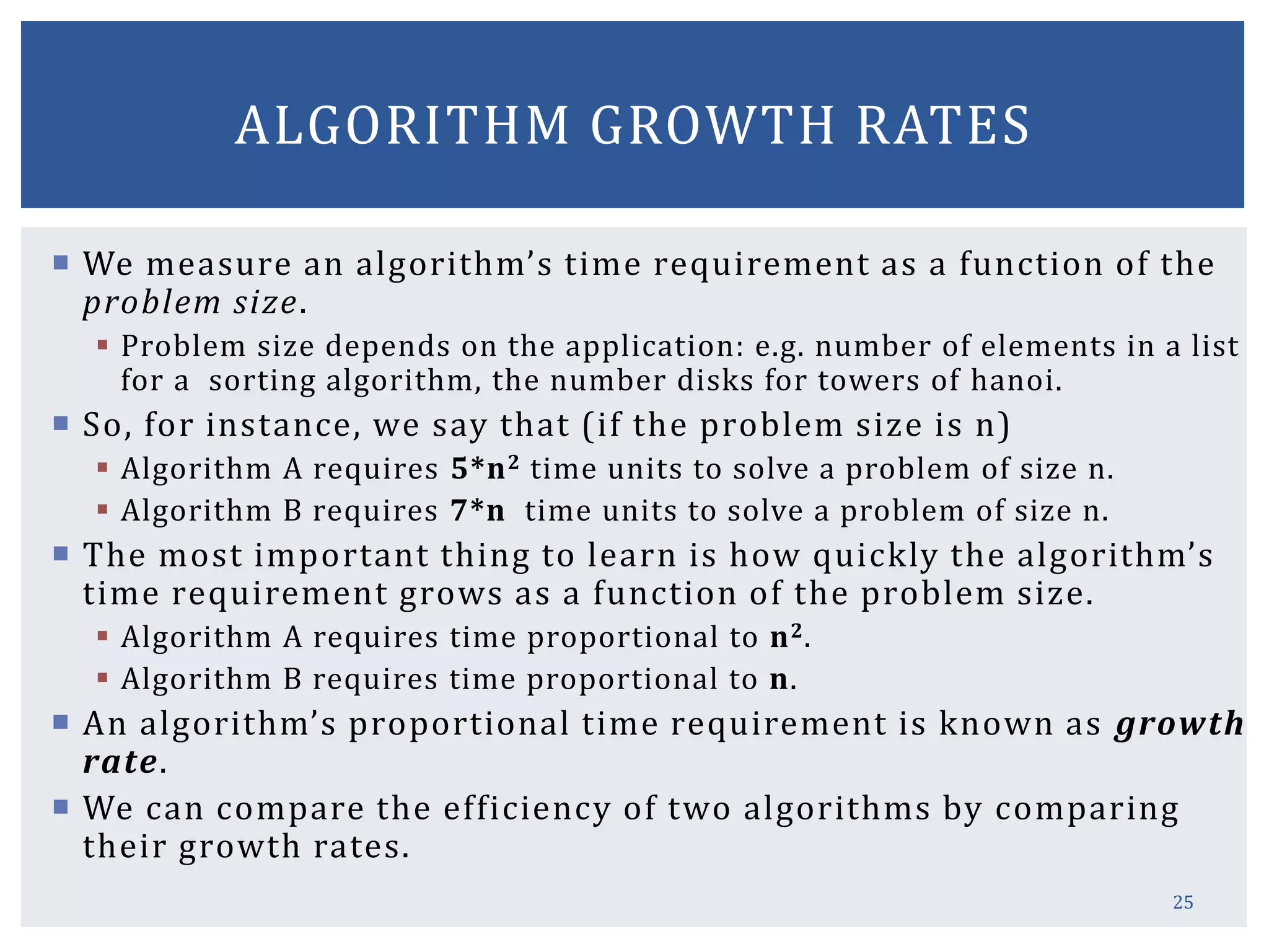
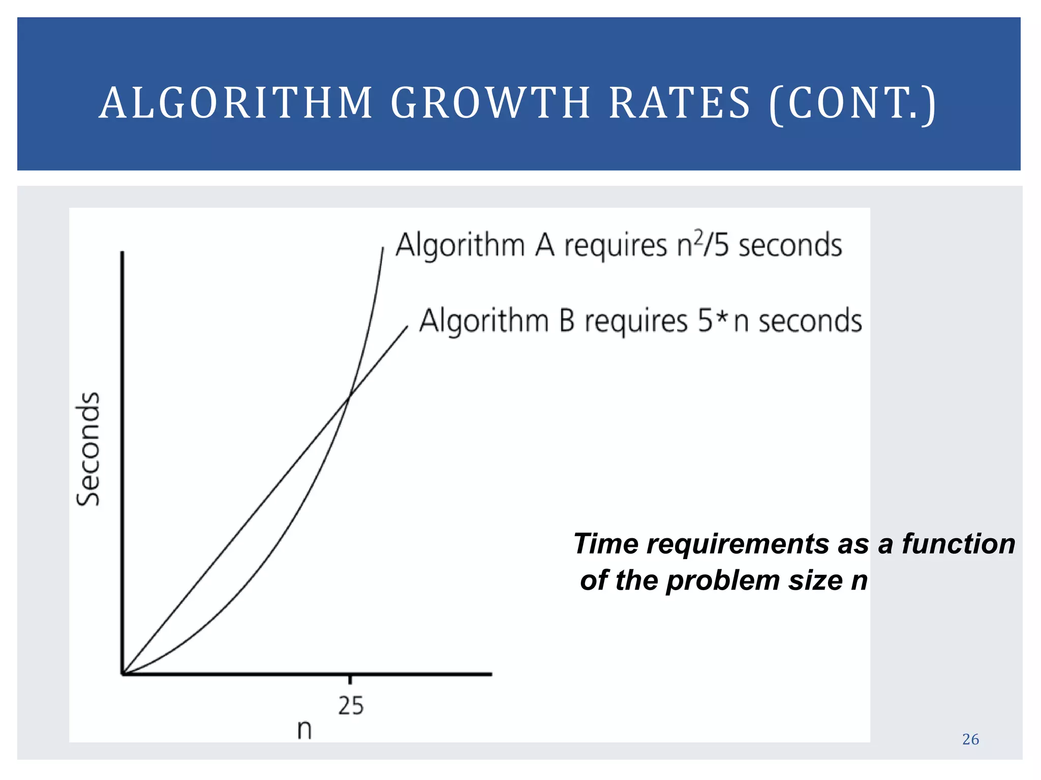
ALGORITHM GROWTH RATES
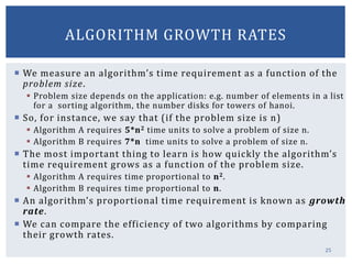
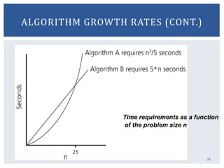
 We measure an algorithm’s time requirement as a function of the
problem size.
 Problem size depends on the application: e.g. number of elements in a list
for a sorting algorithm, the number disks for towers of hanoi.
 So, for instance, we say that (if the problem size is n)
 Algorithm A requires 5*n2 time units to solve a problem of size n.
 Algorithm B requires 7*n time units to solve a problem of size n.
 The most important thing to learn is how quickly the algorithm’s
time requirement grows as a function of the problem size.
 Algorithm A requires time proportional to n2.
 Algorithm B requires time proportional to n.
 An algorithm’s proportional time requirement is known as growth
rate.
 We can compare the efficiency of two algorithms by comparing
their growth rates.

26
ALGORITHM GROWTH RATES (CONT.)
Time requirements as a function
of the problem size n

27
COMMON GROWTH RATES
Function Growth Rate Name
c Constant
log N Logarithmic
log2N Log-squared
N Linear
N log N
N2 Quadratic
N3 Cubic
2N Exponential

28
Figure 6.1
Running times for small inputs

29
Figure 6.2
Running times for moderate inputs

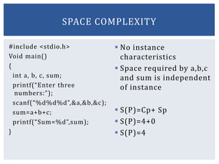
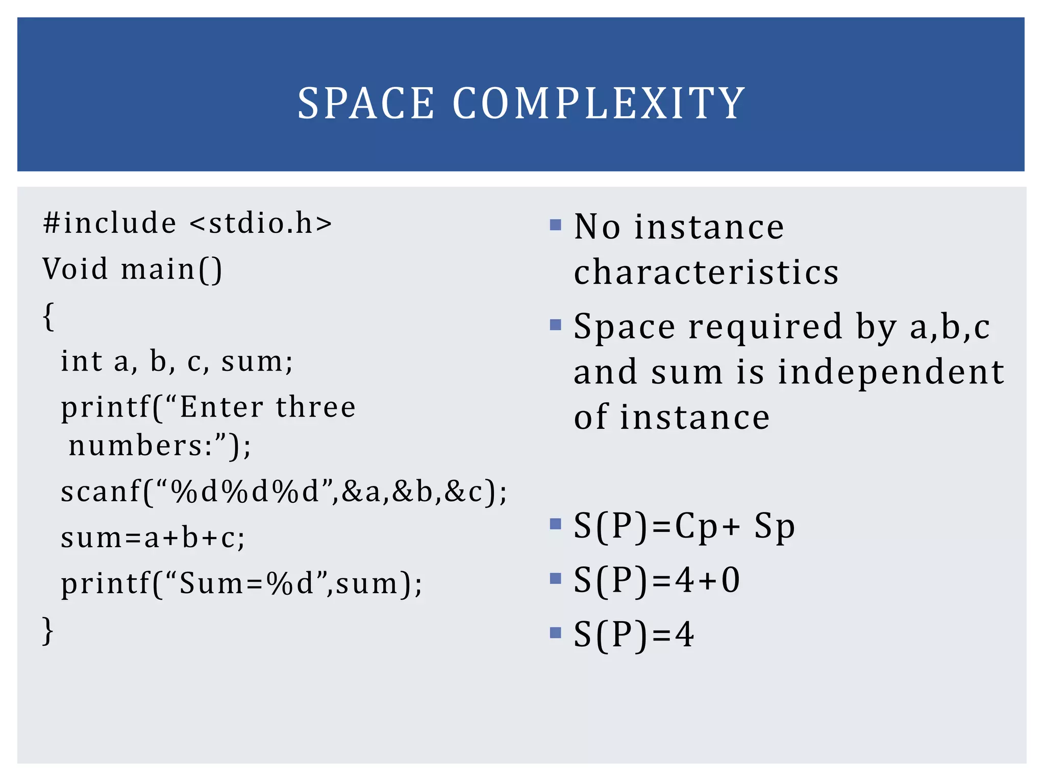
#include <stdio.h>
Void main()
{
int a, b, c, sum;
printf(“Enter three
numbers:”);
scanf(“%d%d%d”,&a,&b,&c);
sum=a+b+c;
printf(“Sum=%d”,sum);
}
 No instance
characteristics
 Space required by a,b,c
and sum is independent
of instance
 S(P)=Cp+ Sp
 S(P)=4+0
 S(P)=4
SPACE COMPLEXITY

int add(int x[], int n)
{
int total=0,i;
for(i=0;i<n;i++)
total=total+x[i];
return total;
}
 Instance = n
 Space required by total,
i, n: 3
 Space required by
constant: 1
 S(P)=Cp+ Sp
 S(P)=3+1+n
 S(P)=4+n
SPACE COMPLEXITY

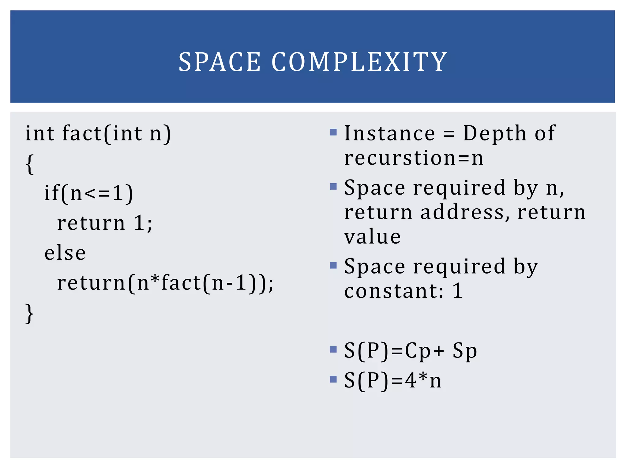
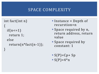
int fact(int n)
{
if(n<=1)
return 1;
else
return(n*fact(n-1));
}
 Instance = Depth of
recurstion=n
 Space required by n,
return address, return
value
 Space required by
constant: 1
 S(P)=Cp+ Sp
 S(P)=4*n
SPACE COMPLEXITY

Unit i basic concepts of algorithms

In this document

More Related Content

What's hot

Similar to Unit i basic concepts of algorithms

Recently uploaded

Unit i basic concepts of algorithms