Downloaded 23 times


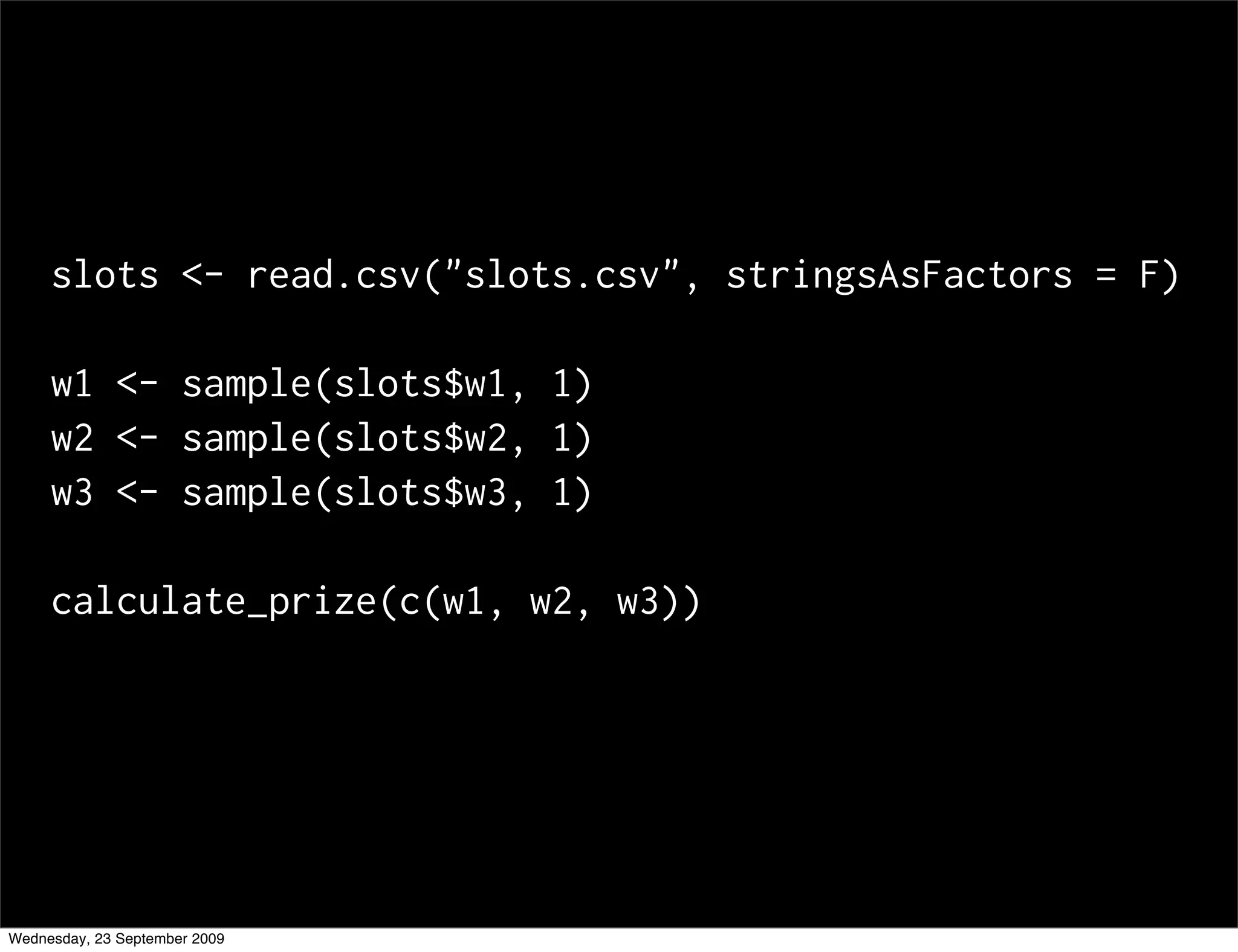
![calculate_prize <- function(windows) {
payoffs <- c("DD" = 800, "7" = 80, "BBB" = 40,
"BB" = 25, "B" = 10, "C" = 10, "0" = 0)
same <- length(unique(windows)) == 1
allbars <- all(windows %in% c("B", "BB", "BBB"))
if (same) {
prize <- payoffs[windows[1]]
} else if (allbars) {
prize <- 5
} else {
cherries <- sum(windows == "C")
diamonds <- sum(windows == "DD")
prize <- c(0, 2, 5)[cherries + 1] *
c(1, 2, 4)[diamonds + 1]
}
prize
}
Wednesday, 23 September 2009](https://image.slidesharecdn.com/09-simulation-090923150302-phpapp01/85/09-Simulation-5-320.jpg)

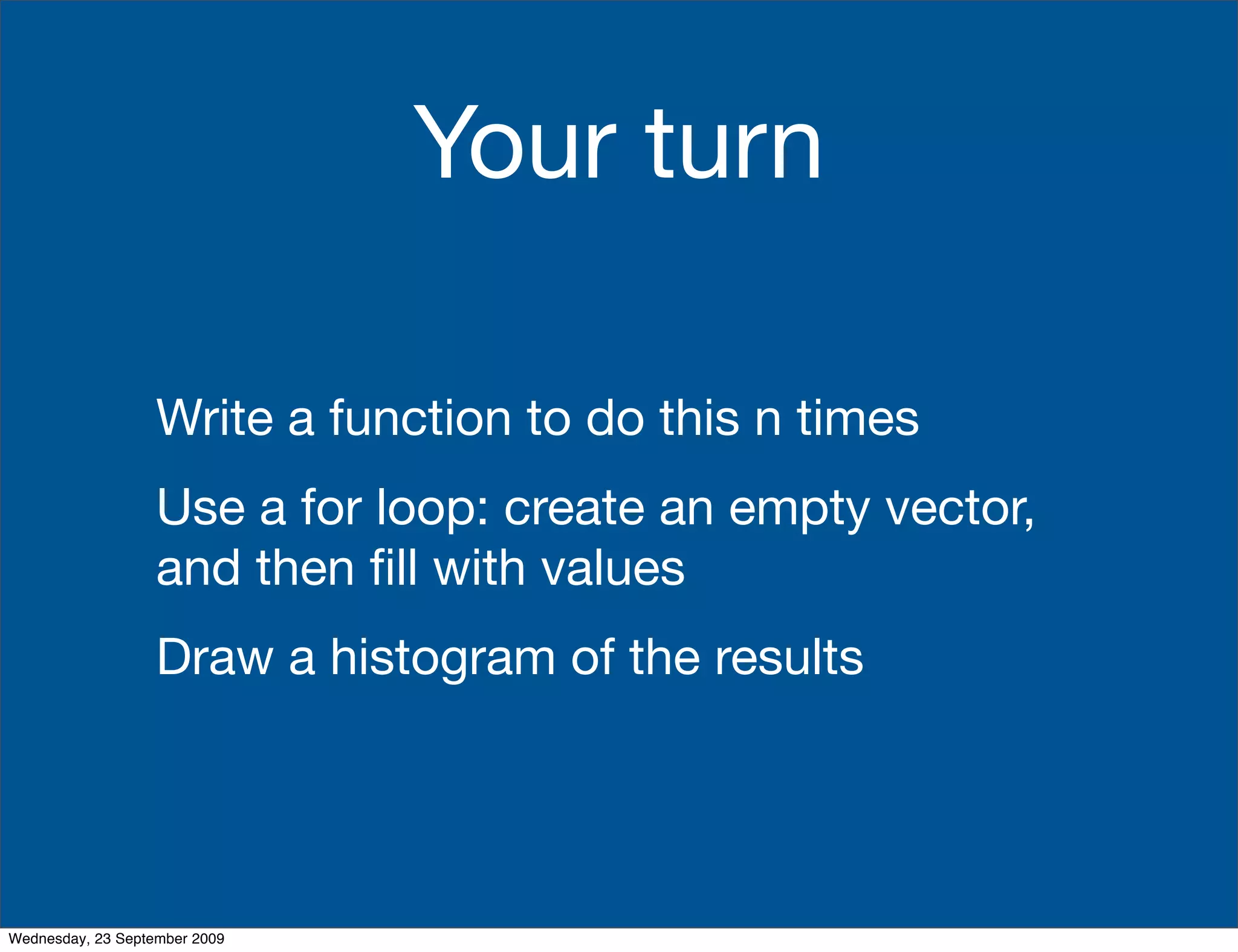
![n <- 100
prizes <- rep(NA, n)
for(i in seq_along(prizes)) {
prizes[i] <- random_prize()
}
Wednesday, 23 September 2009](https://image.slidesharecdn.com/09-simulation-090923150302-phpapp01/85/09-Simulation-10-320.jpg)
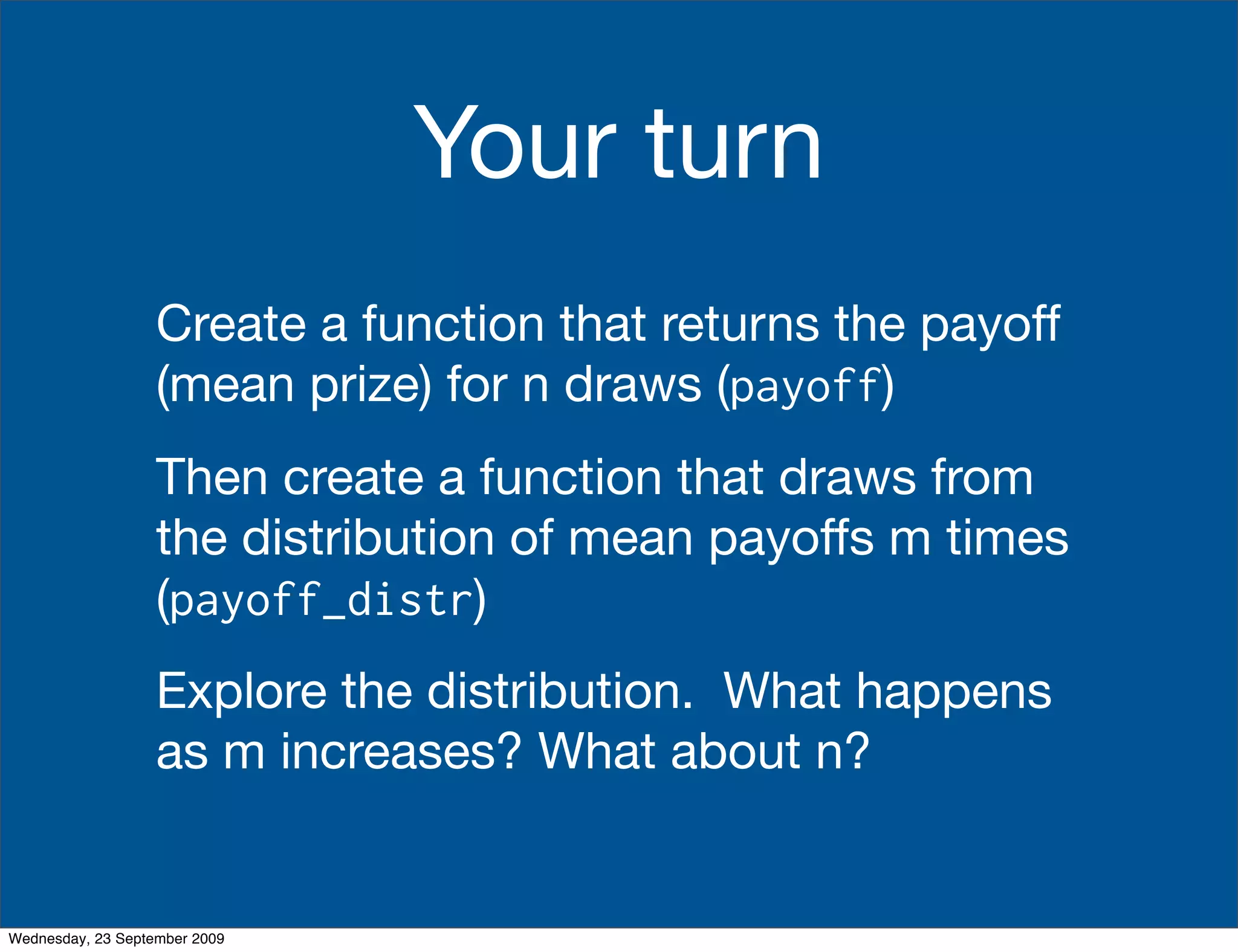
![random_prizes <- function(n) {
prizes <- rep(NA, n)
for(i in seq_along(prizes)) {
prizes[i] <- random_prize()
}
prizes
}
library(ggplot2)
qplot(random_prizes(100))
Wednesday, 23 September 2009](https://image.slidesharecdn.com/09-simulation-090923150302-phpapp01/85/09-Simulation-11-320.jpg)
![payoff <- function(n) {
mean(random_prizes(n))
}
m <- 100
n <- 10
payoffs <- rep(NA, m)
for(i in seq_along(payoffs)) {
payoffs[i] <- payoff(n)
}
qplot(payoffs, binwidth = 0.1)
Wednesday, 23 September 2009](https://image.slidesharecdn.com/09-simulation-090923150302-phpapp01/85/09-Simulation-13-320.jpg)
![payoff_distr <- function(m, n) {
payoffs <- rep(NA, m)
for(i in seq_along(payoffs)) {
payoffs[i] <- payoff(n)
}
payoffs
}
dist <- payoff_distr(100, 1000)
qplot(dist, binwidth = 0.05)
Wednesday, 23 September 2009](https://image.slidesharecdn.com/09-simulation-090923150302-phpapp01/85/09-Simulation-14-320.jpg)
![# Speeding things up a bit
system.time(payoff_distr(200, 100))
payoff <- function(n) {
w1 <- sample(slots$w1, n, rep = T)
w2 <- sample(slots$w2, n, rep = T)
w3 <- sample(slots$w2, n, rep = T)
prizes <- rep(NA, n)
for(i in seq_along(prizes)) {
prizes[i] <- calculate_prize(c(w1[i], w2[i], w3[i]))
}
mean(prizes)
}
system.time(payoff_distr(200, 100))
Wednesday, 23 September 2009](https://image.slidesharecdn.com/09-simulation-090923150302-phpapp01/85/09-Simulation-15-320.jpg)


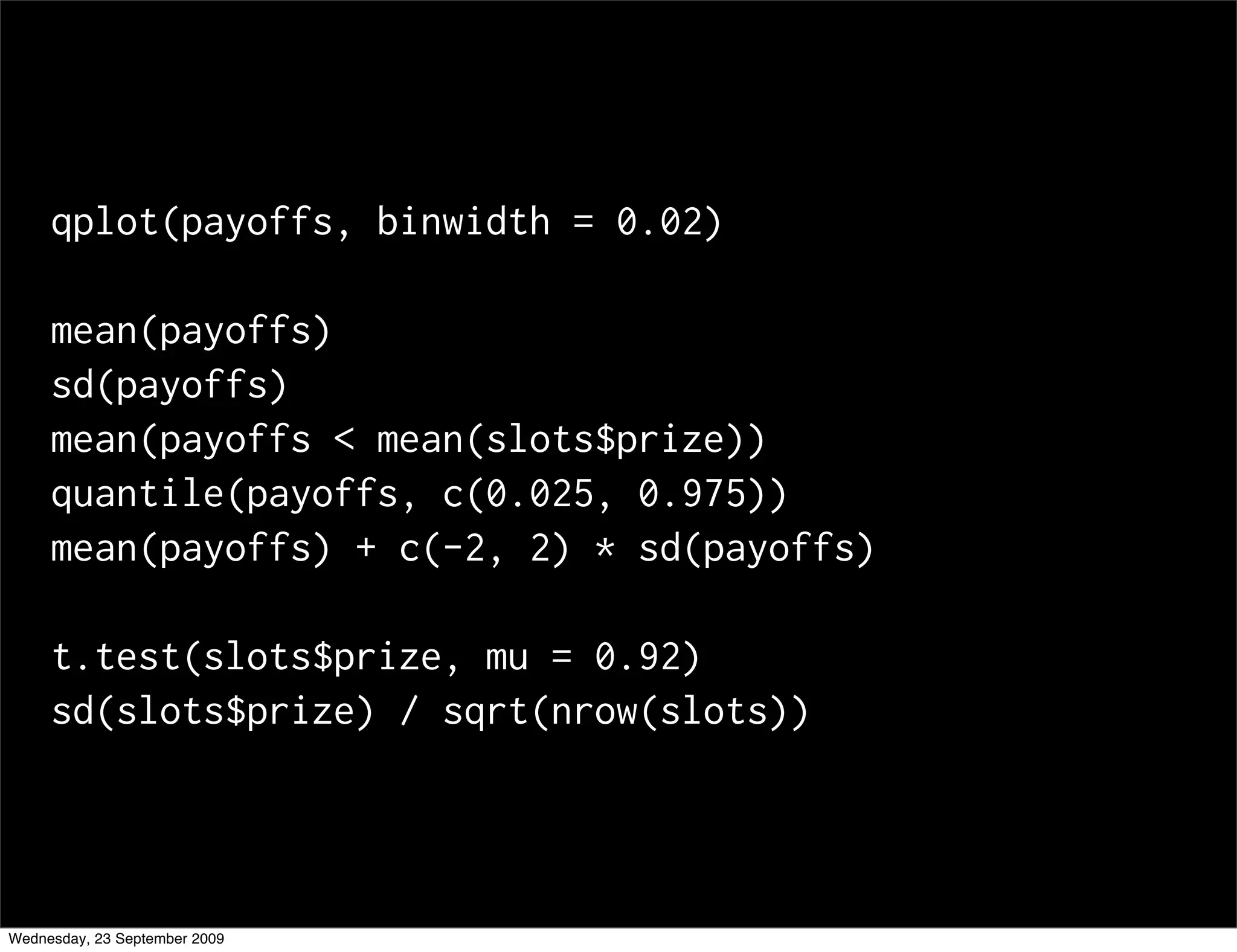
![poss <- with(distdf, expand.grid(
w1 = slot, w2 = slot, w3 = slot,
stringsAsFactors = FALSE
))
poss$prize <- NA
for(i in seq_len(nrow(poss))) {
window <- as.character(poss[i, 1:3])
poss$prize[i] <- calculate_prize(window)
}
Wednesday, 23 September 2009](https://image.slidesharecdn.com/09-simulation-090923150302-phpapp01/85/09-Simulation-20-320.jpg)
![poss$prob <- with(poss,
dist[w1] * dist[w2] * dist[w3])
(poss_mean <- with(poss, sum(prob * prize)))
# How do we determine the variance of this
# estimator?
Wednesday, 23 September 2009](https://image.slidesharecdn.com/09-simulation-090923150302-phpapp01/85/09-Simulation-22-320.jpg)


![calculate_prize <- function(windows) {
payoffs <- c("DD" = 800, "7" = 80, "BBB" = 40,
"BB" = 25, "B" = 10, "C" = 10, "0" = 0)
same <- length(unique(windows)) == 1
allbars <- all(windows %in% c("B", "BB", "BBB"))
if (same) {
prize <- payoffs[windows[1]]
} else if (allbars) {
prize <- 5
} else {
cherries <- sum(windows == "C")
diamonds <- sum(windows == "DD")
prize <- c(0, 2, 5)[cherries + 1] *
c(1, 2, 4)[diamonds + 1]
}
prize
}
Wednesday, 23 September 2009](https://image.slidesharecdn.com/09-simulation-090923150302-phpapp01/75/09-Simulation-5-2048.jpg)

![n <- 100
prizes <- rep(NA, n)
for(i in seq_along(prizes)) {
prizes[i] <- random_prize()
}
Wednesday, 23 September 2009](https://image.slidesharecdn.com/09-simulation-090923150302-phpapp01/75/09-Simulation-10-2048.jpg)
![random_prizes <- function(n) {
prizes <- rep(NA, n)
for(i in seq_along(prizes)) {
prizes[i] <- random_prize()
}
prizes
}
library(ggplot2)
qplot(random_prizes(100))
Wednesday, 23 September 2009](https://image.slidesharecdn.com/09-simulation-090923150302-phpapp01/75/09-Simulation-11-2048.jpg)
![payoff <- function(n) {
mean(random_prizes(n))
}
m <- 100
n <- 10
payoffs <- rep(NA, m)
for(i in seq_along(payoffs)) {
payoffs[i] <- payoff(n)
}
qplot(payoffs, binwidth = 0.1)
Wednesday, 23 September 2009](https://image.slidesharecdn.com/09-simulation-090923150302-phpapp01/75/09-Simulation-13-2048.jpg)
![payoff_distr <- function(m, n) {
payoffs <- rep(NA, m)
for(i in seq_along(payoffs)) {
payoffs[i] <- payoff(n)
}
payoffs
}
dist <- payoff_distr(100, 1000)
qplot(dist, binwidth = 0.05)
Wednesday, 23 September 2009](https://image.slidesharecdn.com/09-simulation-090923150302-phpapp01/75/09-Simulation-14-2048.jpg)
![# Speeding things up a bit
system.time(payoff_distr(200, 100))
payoff <- function(n) {
w1 <- sample(slots$w1, n, rep = T)
w2 <- sample(slots$w2, n, rep = T)
w3 <- sample(slots$w2, n, rep = T)
prizes <- rep(NA, n)
for(i in seq_along(prizes)) {
prizes[i] <- calculate_prize(c(w1[i], w2[i], w3[i]))
}
mean(prizes)
}
system.time(payoff_distr(200, 100))
Wednesday, 23 September 2009](https://image.slidesharecdn.com/09-simulation-090923150302-phpapp01/75/09-Simulation-15-2048.jpg)

![poss <- with(distdf, expand.grid(
w1 = slot, w2 = slot, w3 = slot,
stringsAsFactors = FALSE
))
poss$prize <- NA
for(i in seq_len(nrow(poss))) {
window <- as.character(poss[i, 1:3])
poss$prize[i] <- calculate_prize(window)
}
Wednesday, 23 September 2009](https://image.slidesharecdn.com/09-simulation-090923150302-phpapp01/75/09-Simulation-20-2048.jpg)
![poss$prob <- with(poss,
dist[w1] * dist[w2] * dist[w3])
(poss_mean <- with(poss, sum(prob * prize)))
# How do we determine the variance of this
# estimator?
Wednesday, 23 September 2009](https://image.slidesharecdn.com/09-simulation-090923150302-phpapp01/75/09-Simulation-22-2048.jpg)

This document discusses simulation methods for analyzing slot machine payout data. It includes sections on the mathematical approach, homework assignments, and feedback. Students are asked to write functions to simulate random slot machine draws, calculate payouts from multiple draws, and explore the distribution of mean payouts from increasing numbers of draws. The document suggests moving from simulation to calculating the expected value and variance of payouts mathematically.


![[112] 모바일 환경에서 실시간 Portrait Segmentation 구현하기](https://cdn.slidesharecdn.com/ss_thumbnails/112-181011023345-thumbnail.jpg?width=600ounds&width=560&fit=bounds)


