Downloaded 132 times
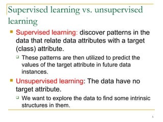
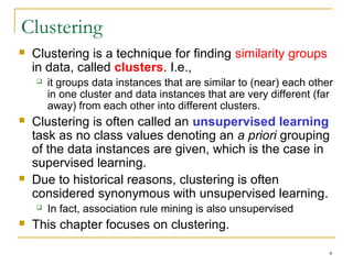
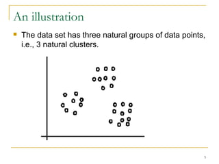
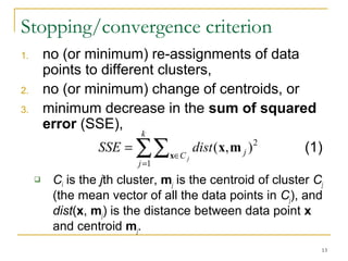
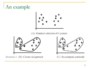
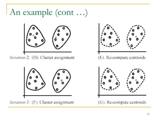
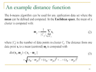


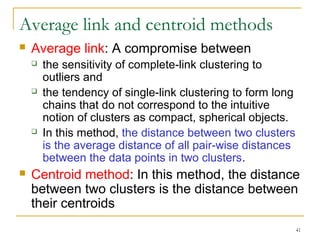

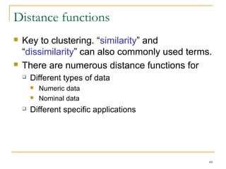
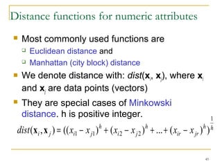

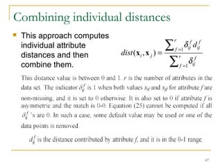
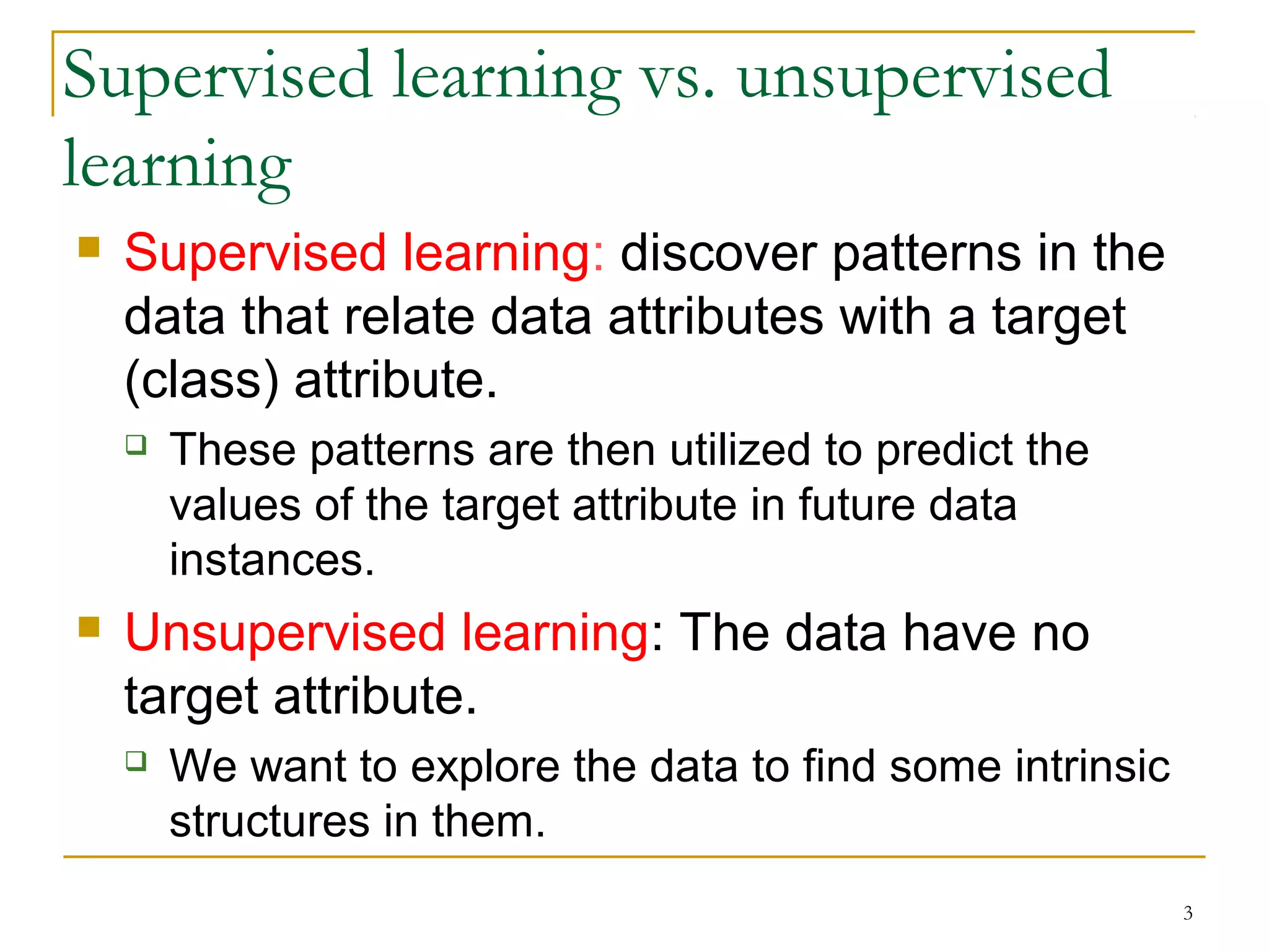
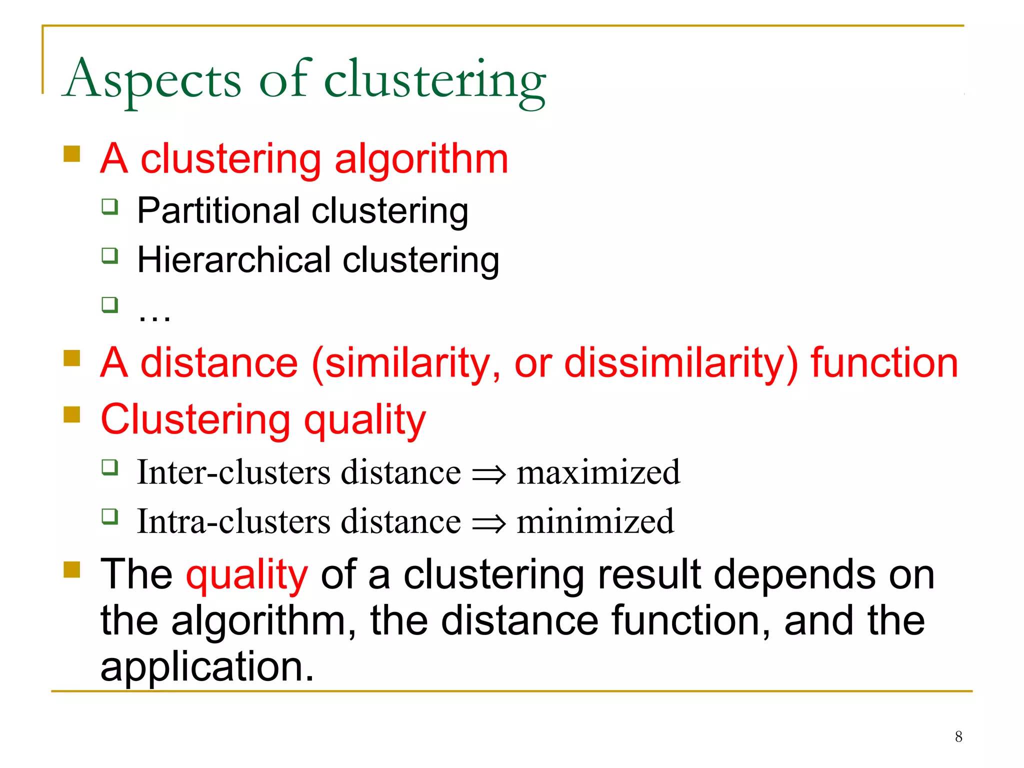
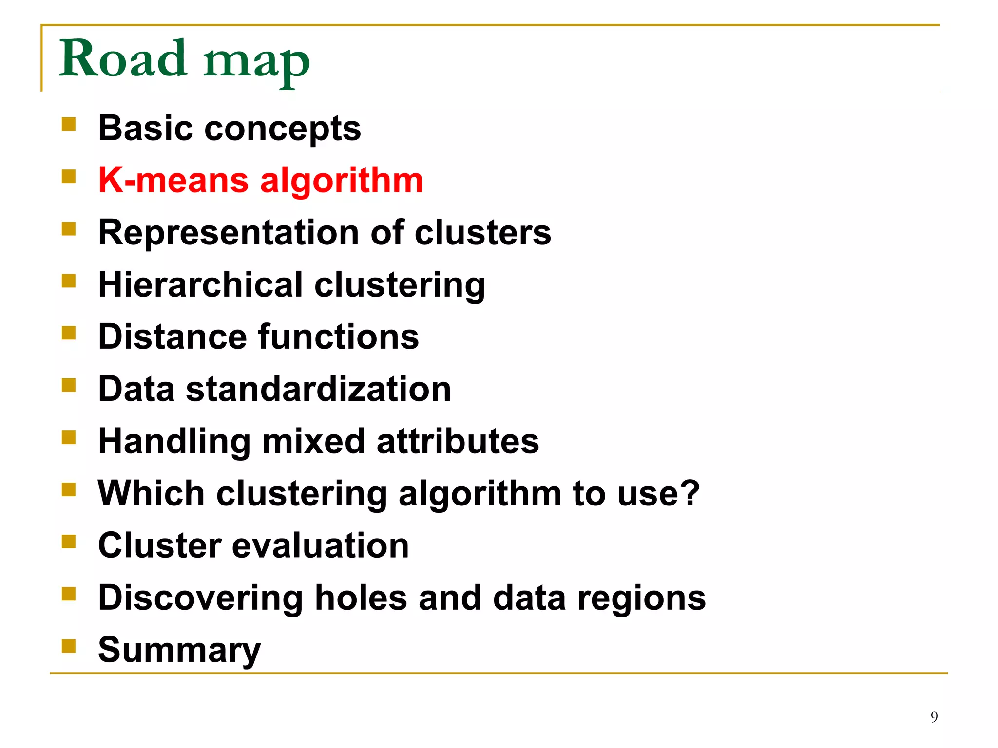
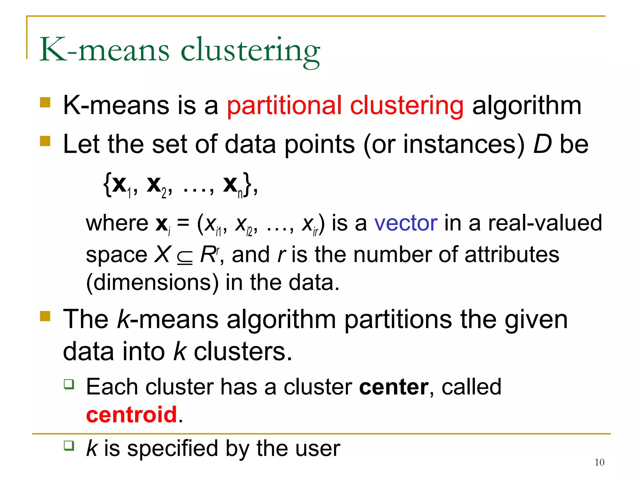
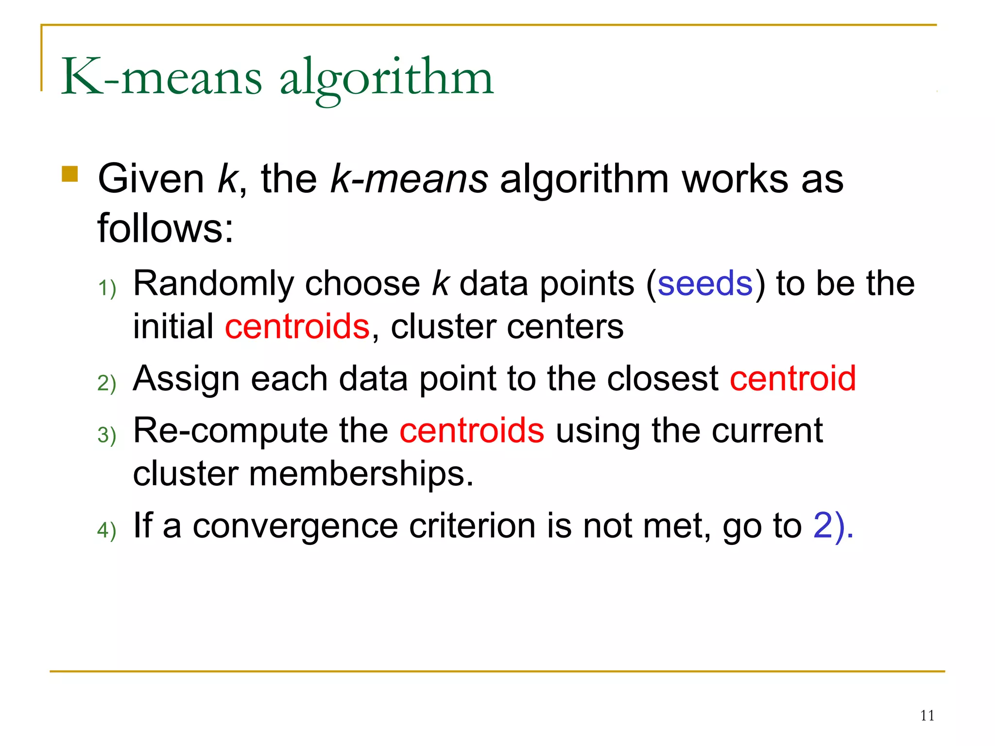
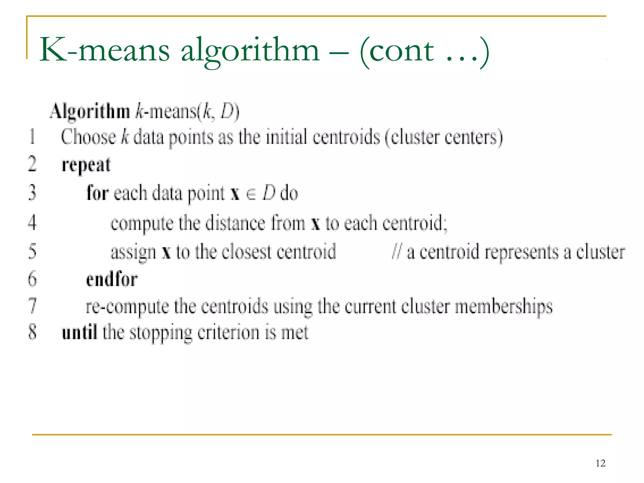
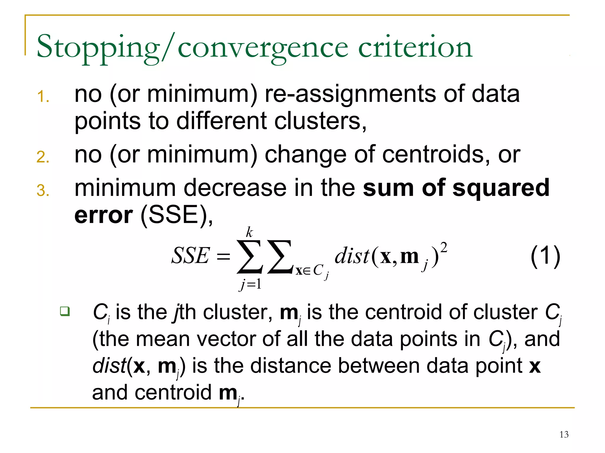
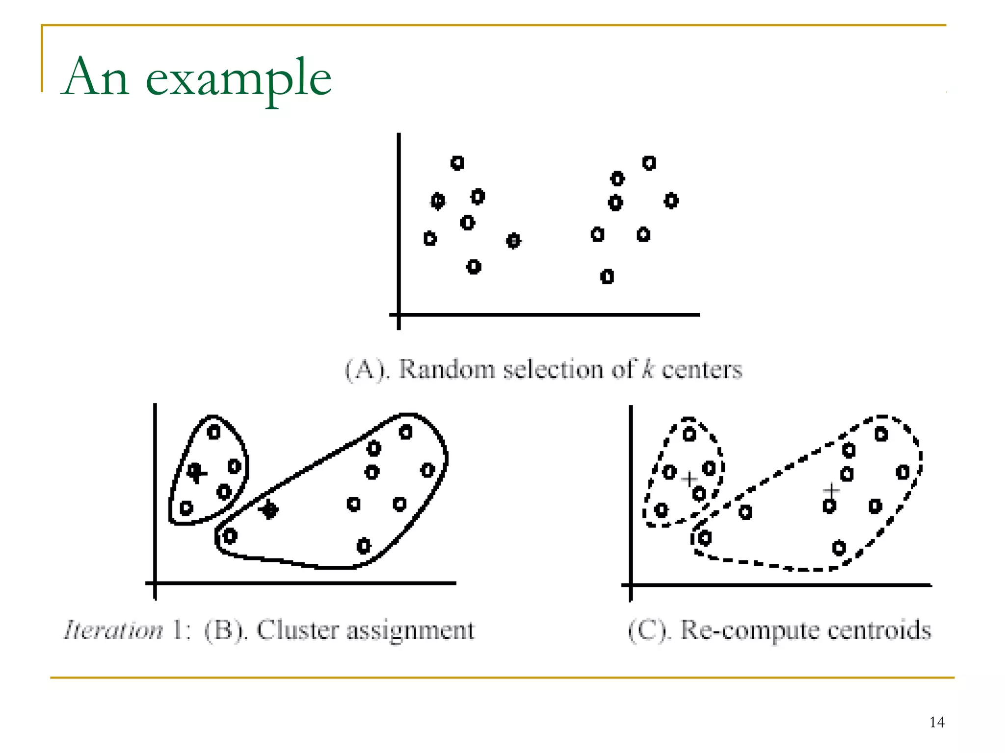
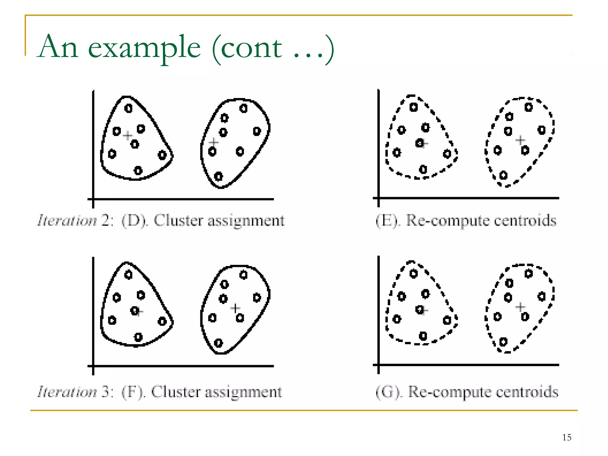
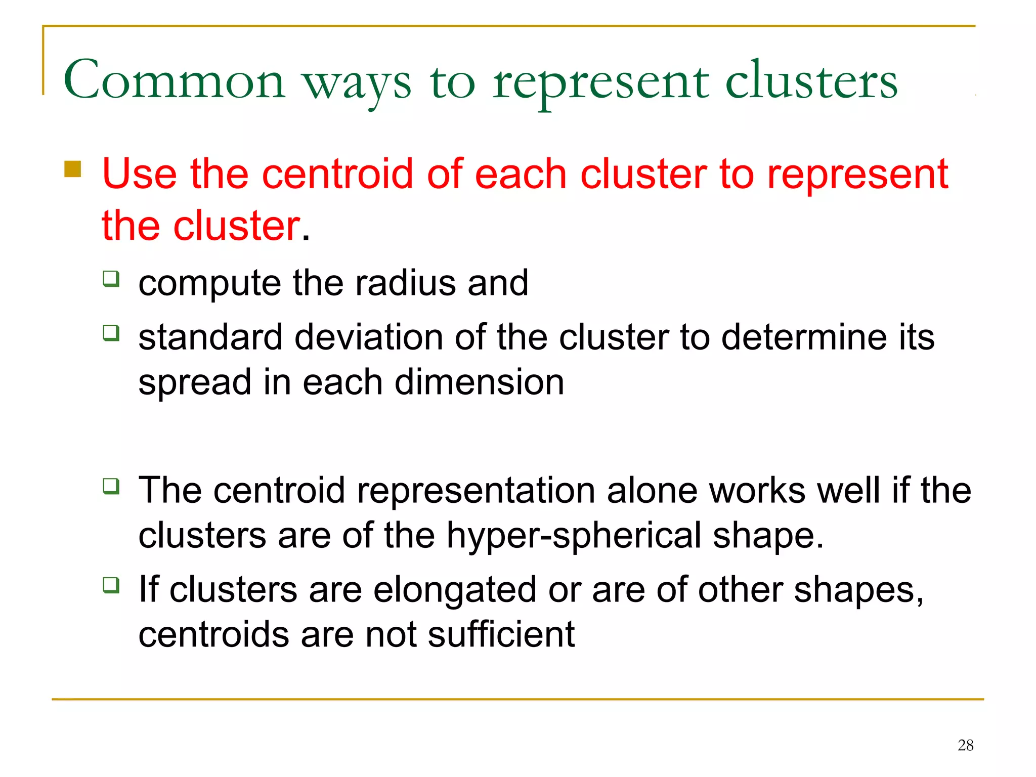
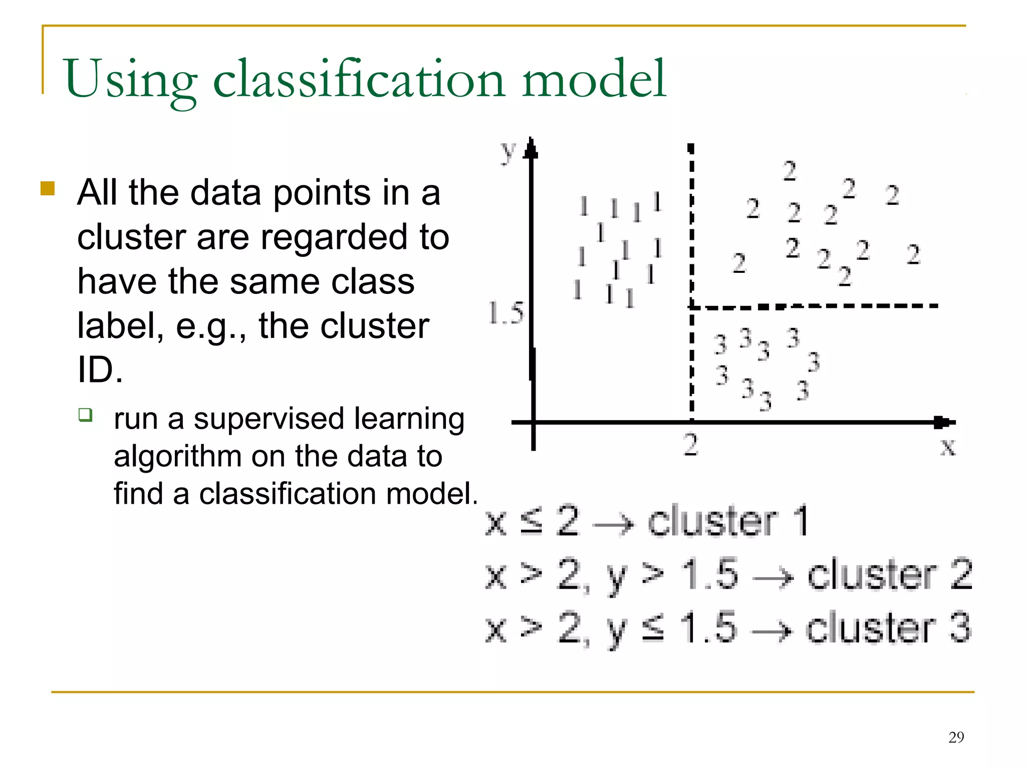

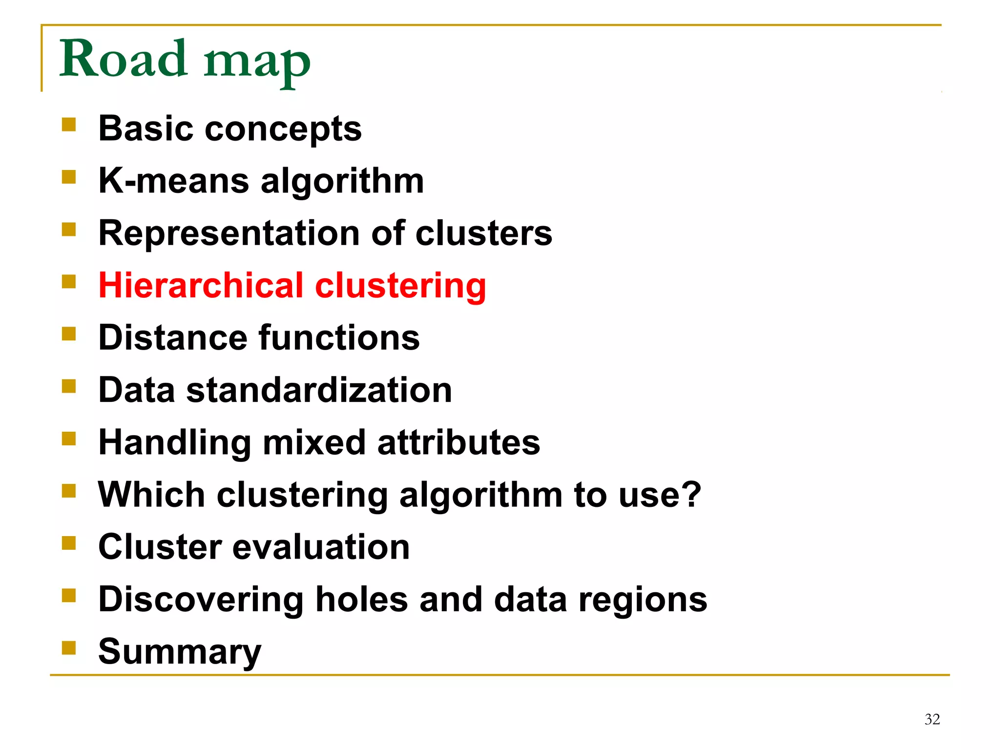
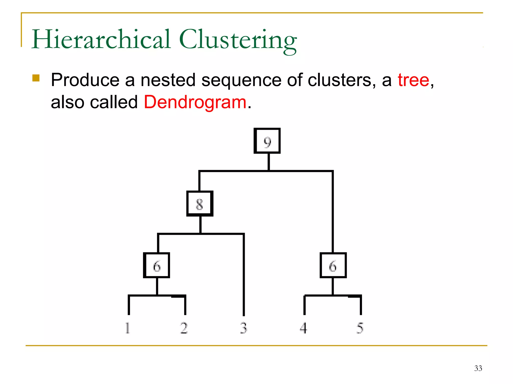
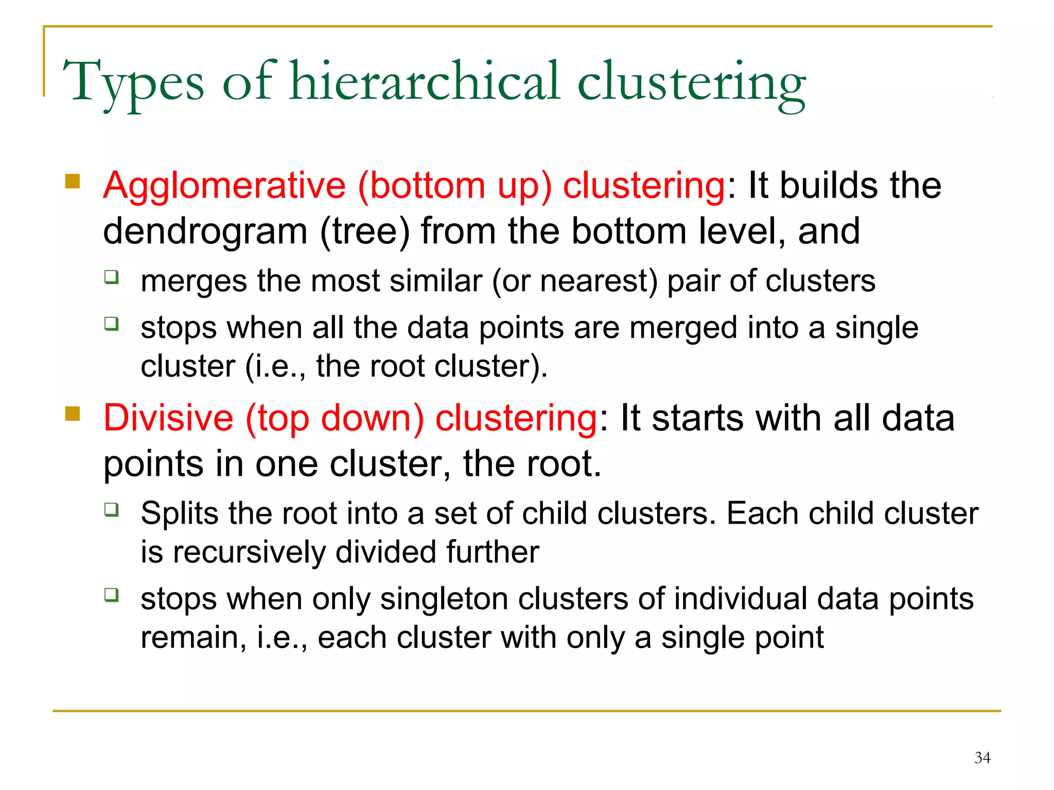
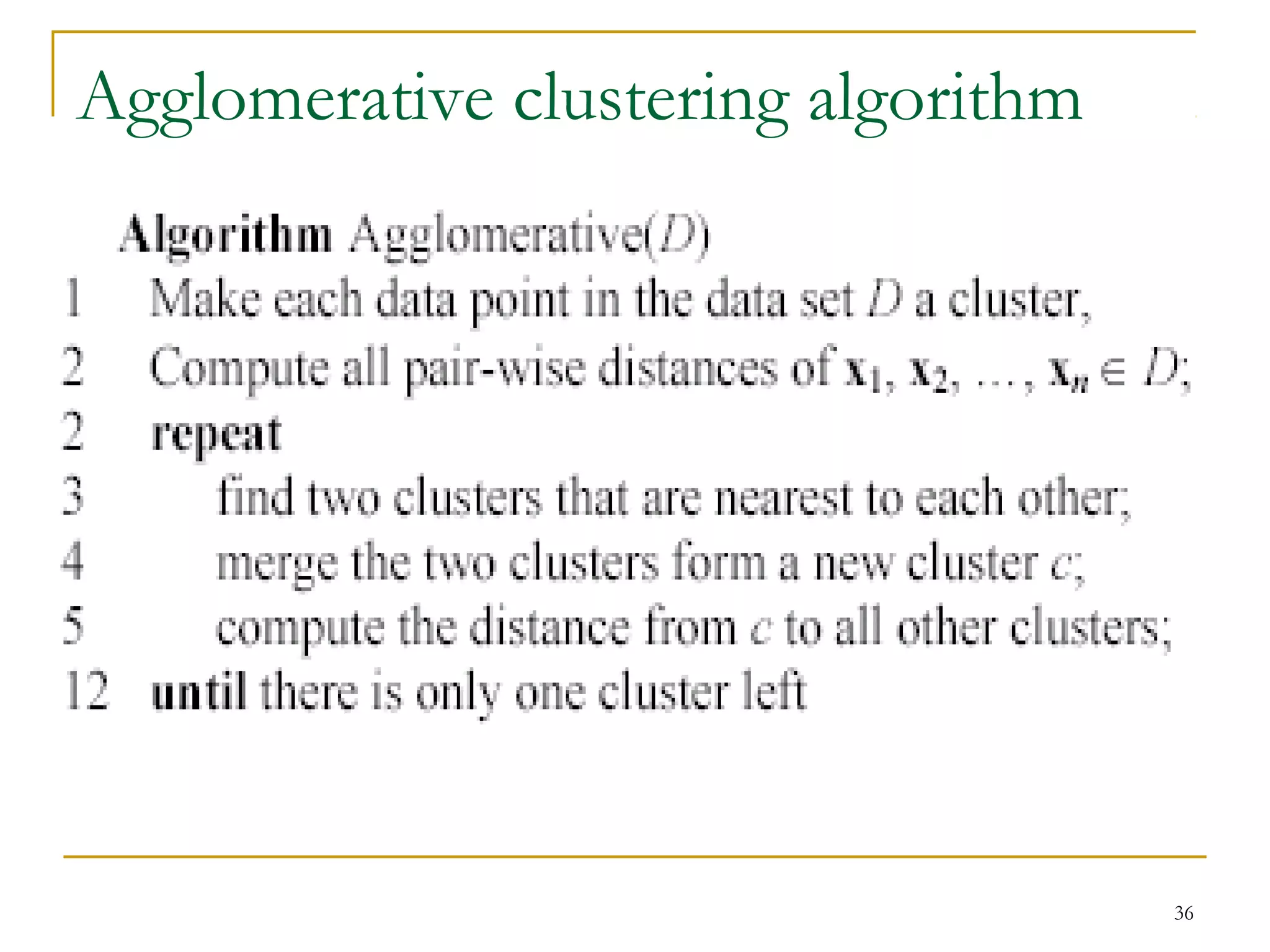

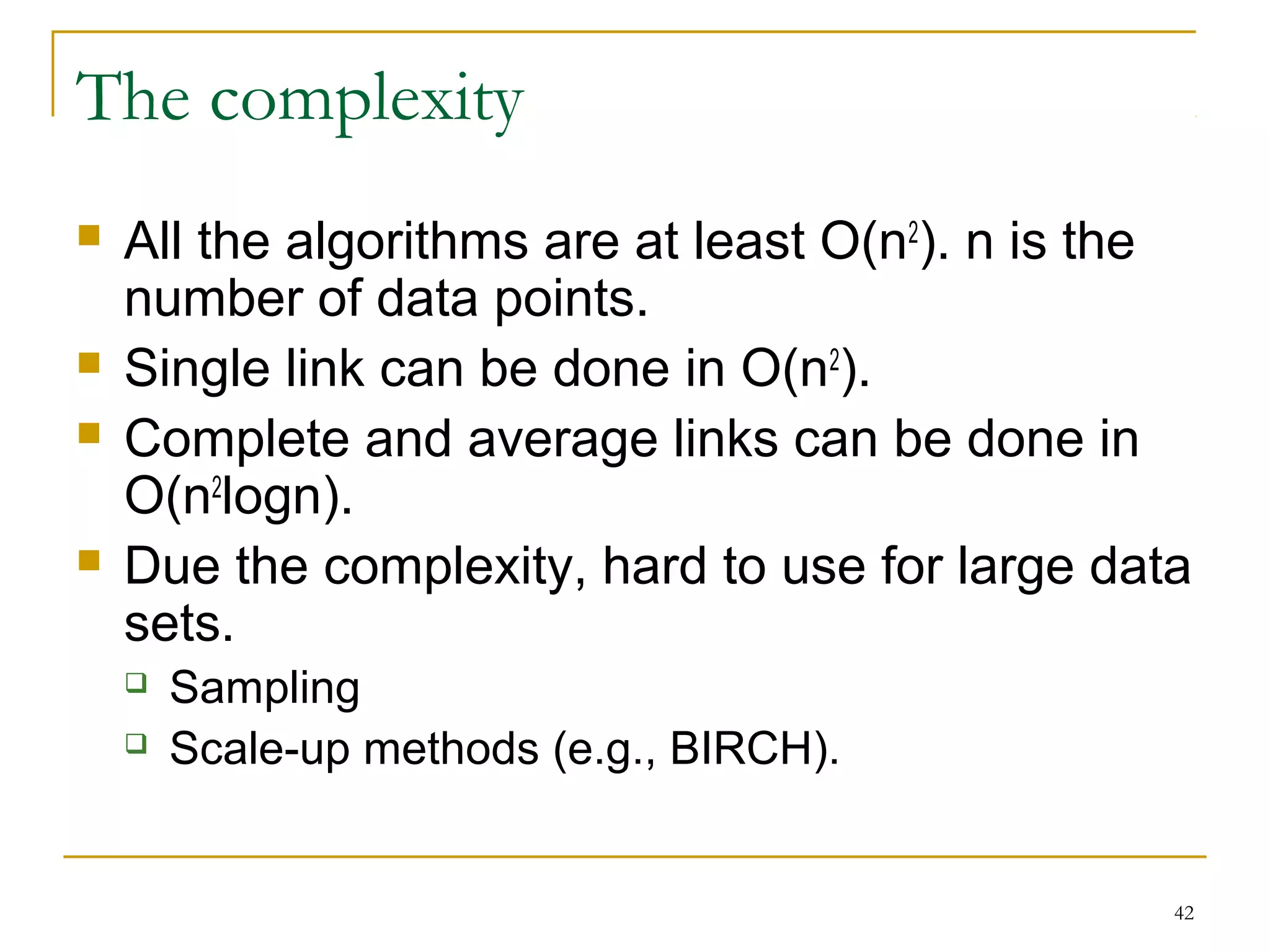
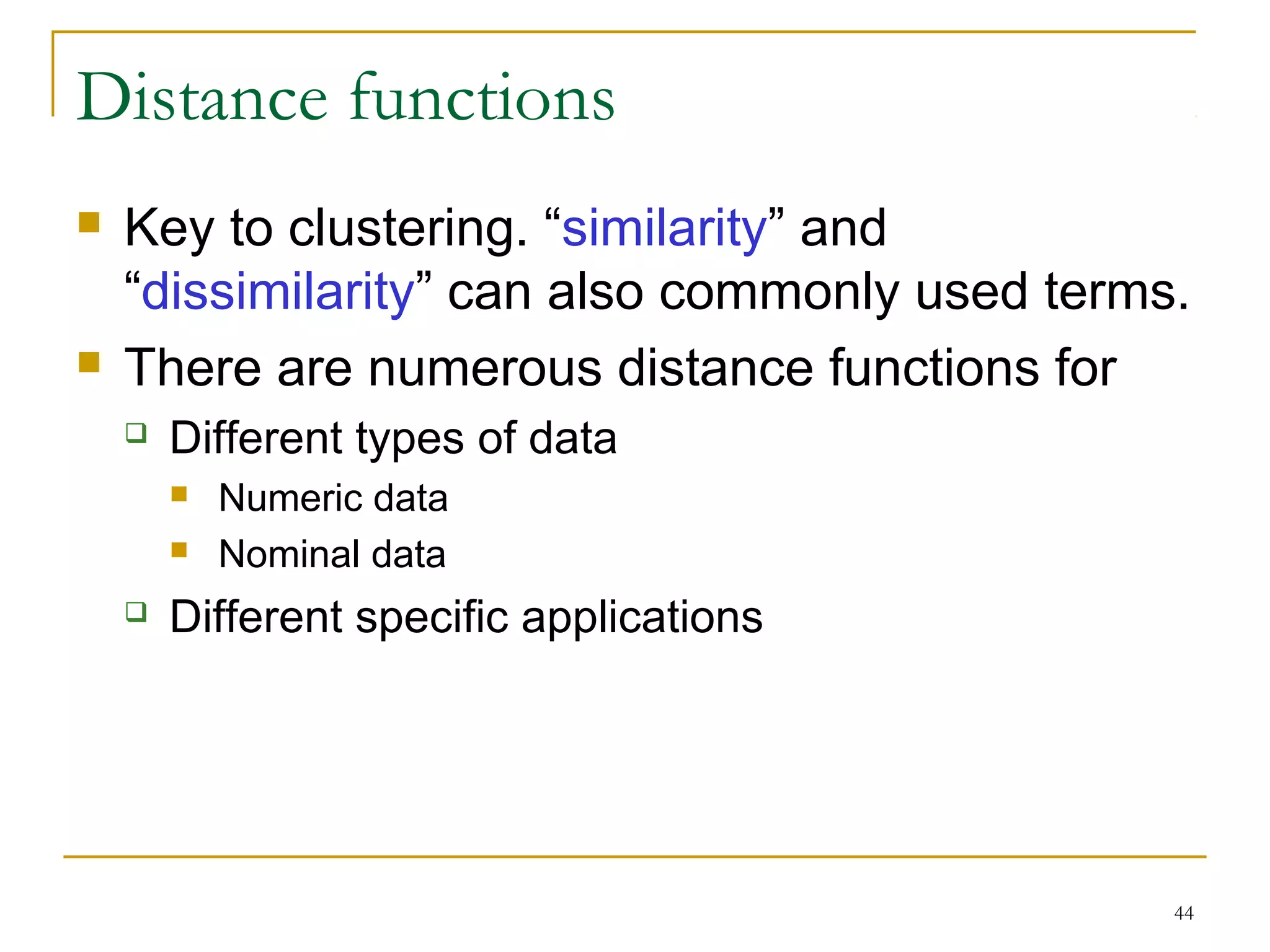

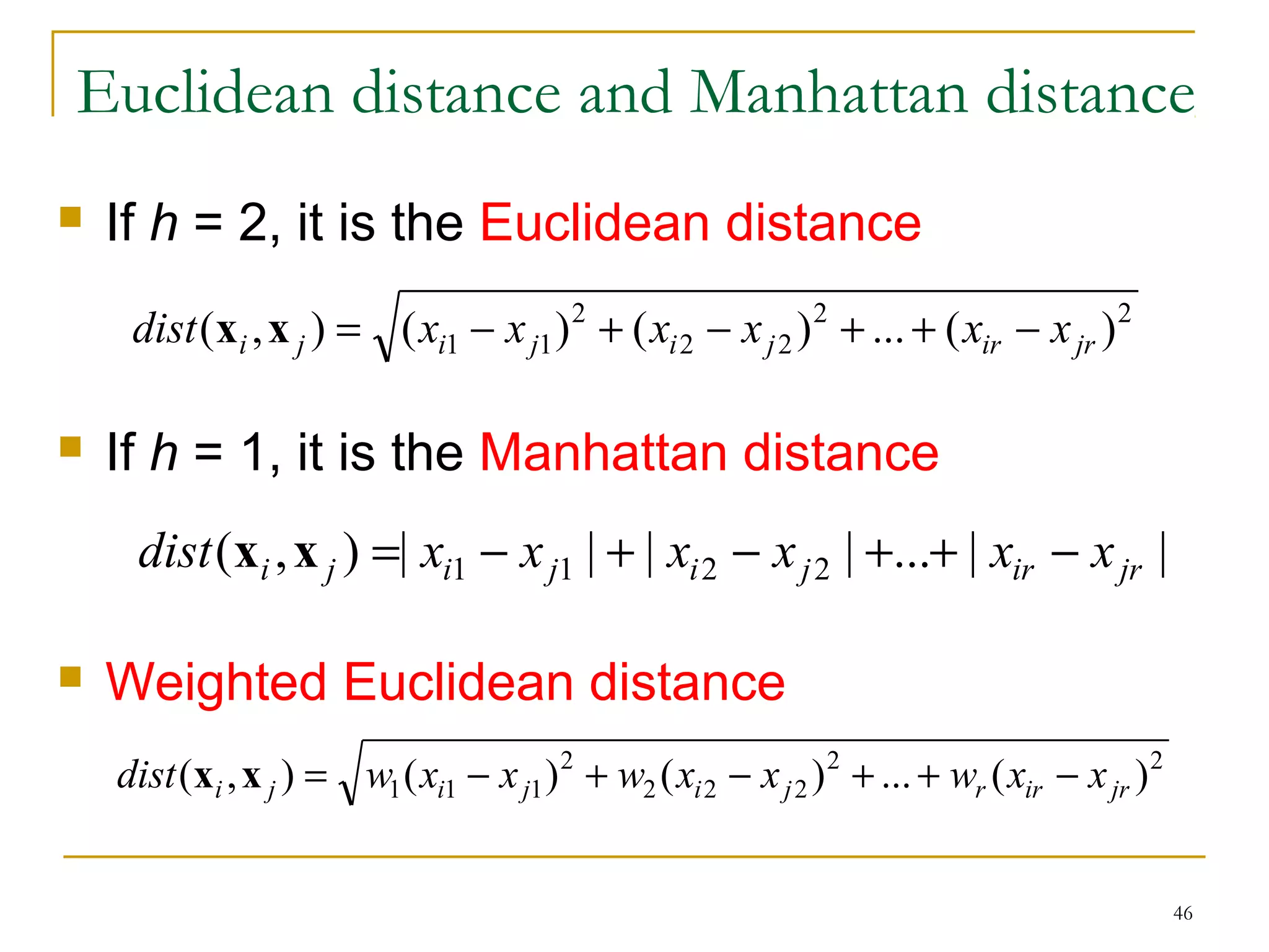

This document provides an overview of supervised and unsupervised learning, with a focus on clustering as an unsupervised learning technique. It describes the basic concepts of clustering, including how clustering groups similar data points together without labeled categories. It then covers two main clustering algorithms - k-means, a partitional clustering method, and hierarchical clustering. It discusses aspects like cluster representation, distance functions, strengths and weaknesses of different approaches. The document aims to introduce clustering and compare it with supervised learning.


![[ML]-Unsupervised-learning_Unit2.ppt.pdf](https://cdn.slidesharecdn.com/ss_thumbnails/ml-unsupervised-learningunit2-230916145038-acbd0397-thumbnail.jpg?width=600ounds&width=560&fit=bounds)


![UiPath Automation Suite Installation (Hands-On) [2/3]](https://cdn.slidesharecdn.com/ss_thumbnails/automationsuitecommunitysession2-251015095633-a6d862f1-thumbnail.jpg?width=600ounds&width=560&fit=bounds)


