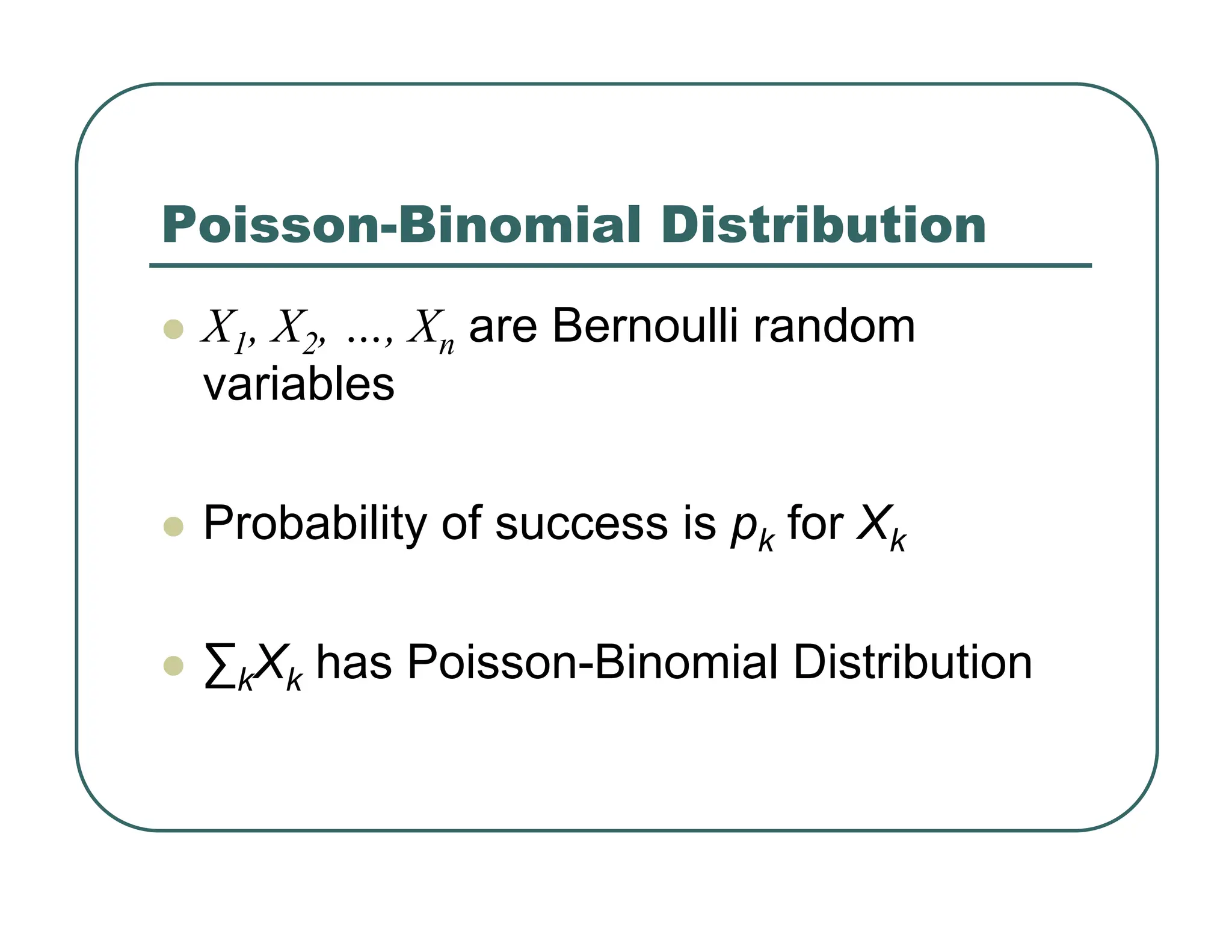
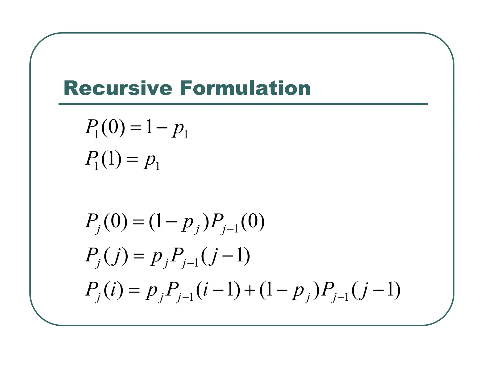
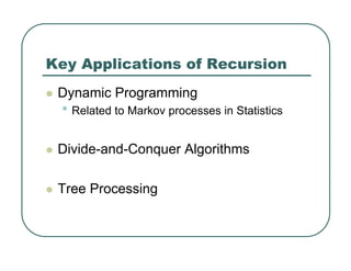
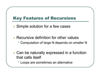
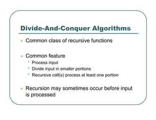
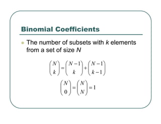
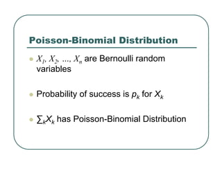
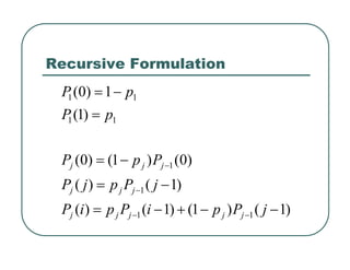
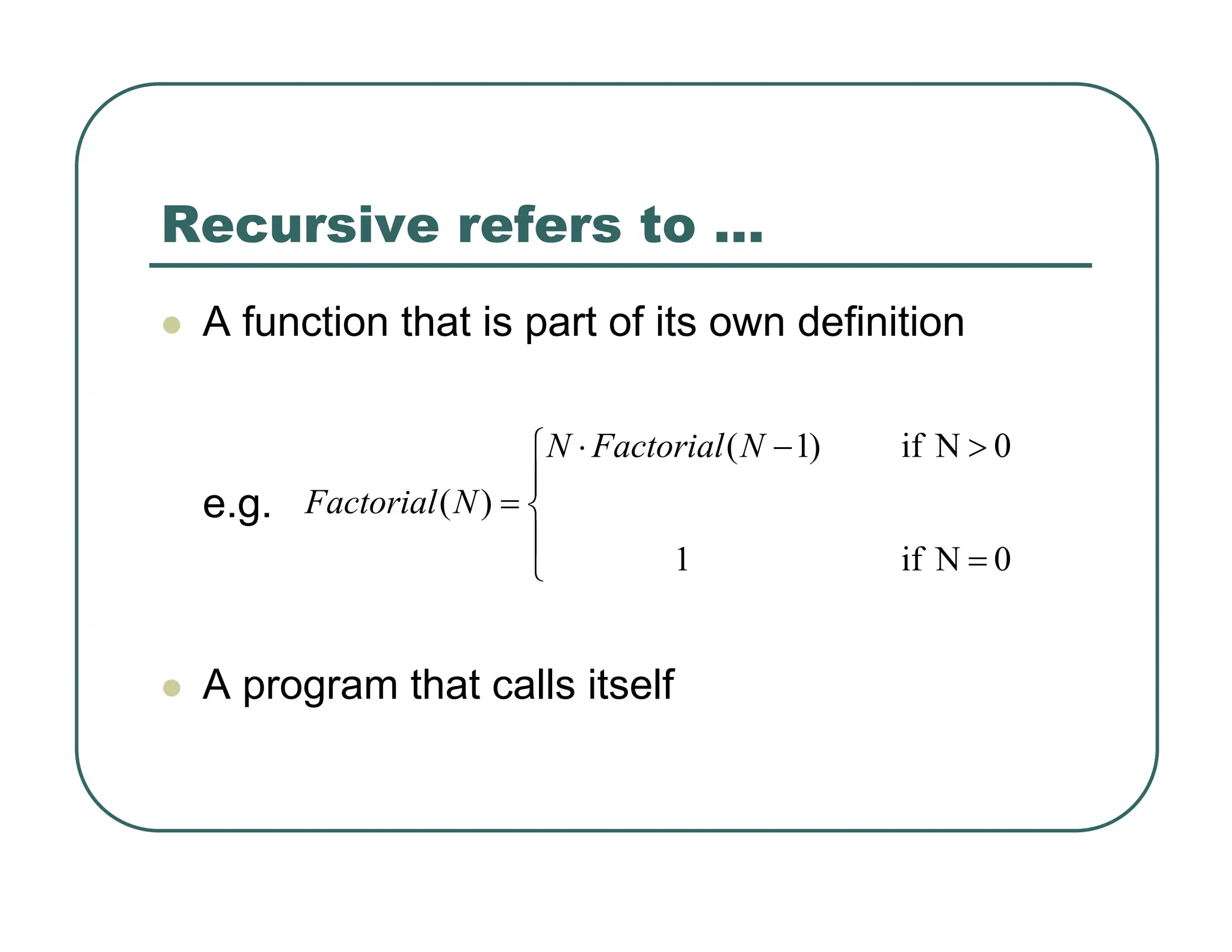
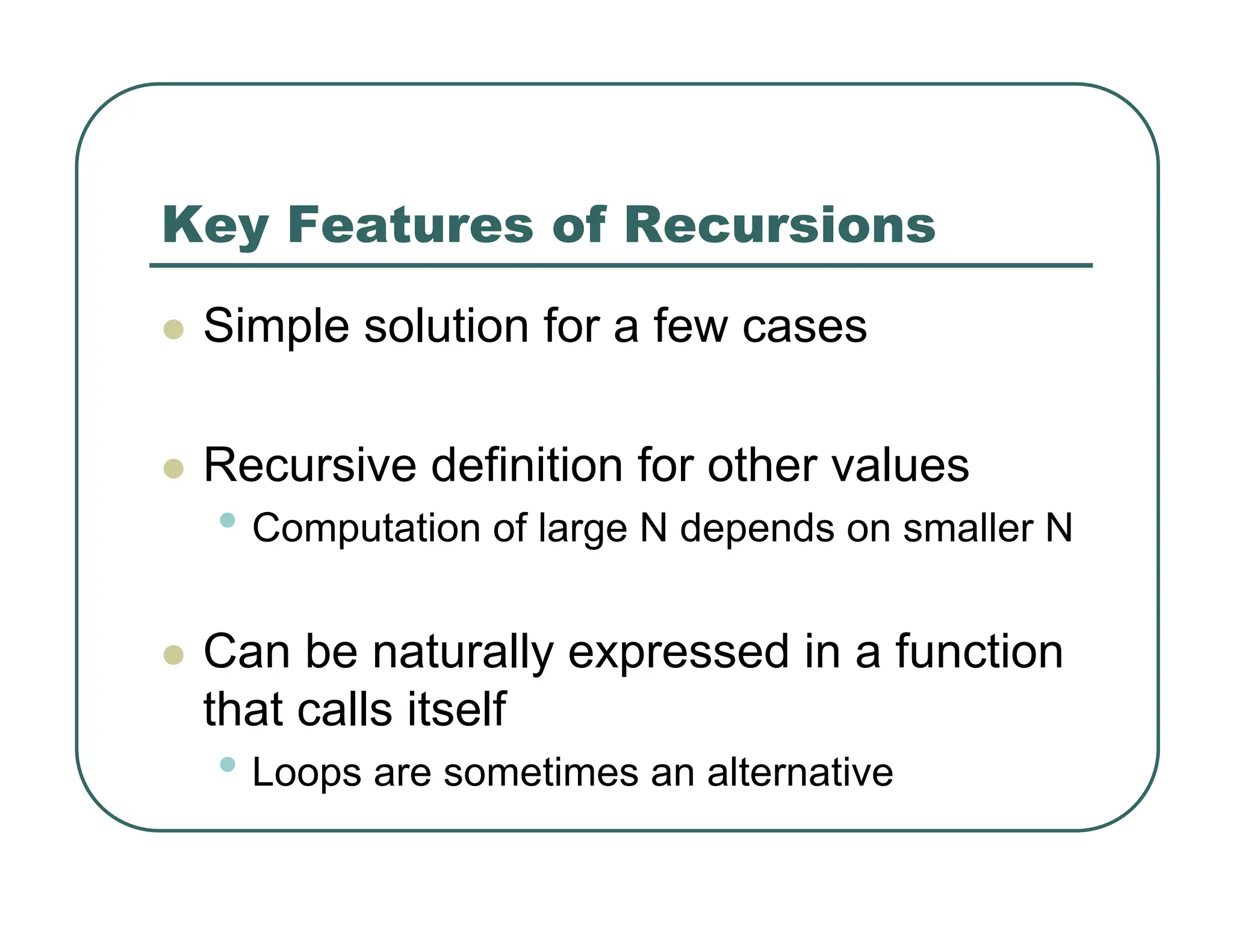
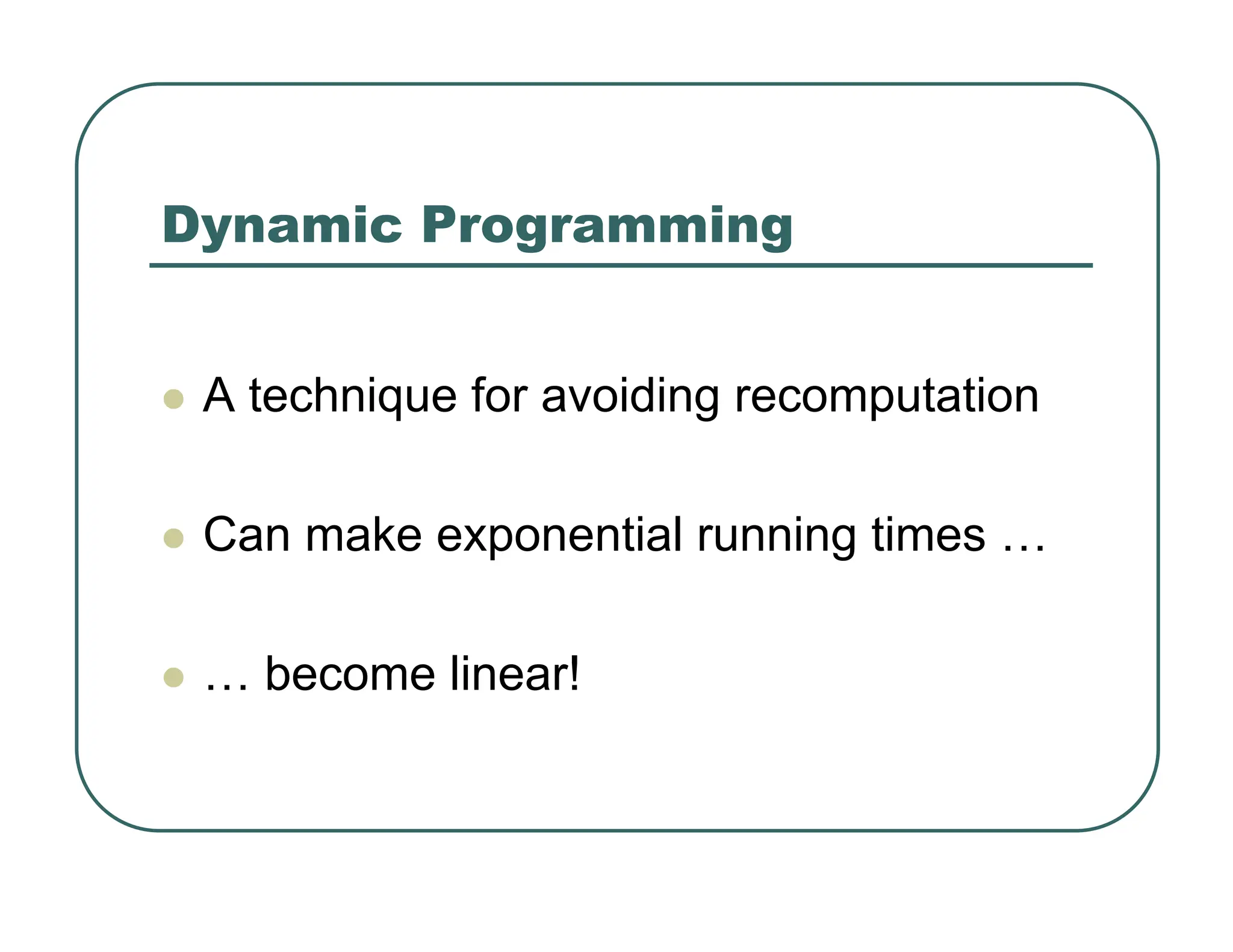
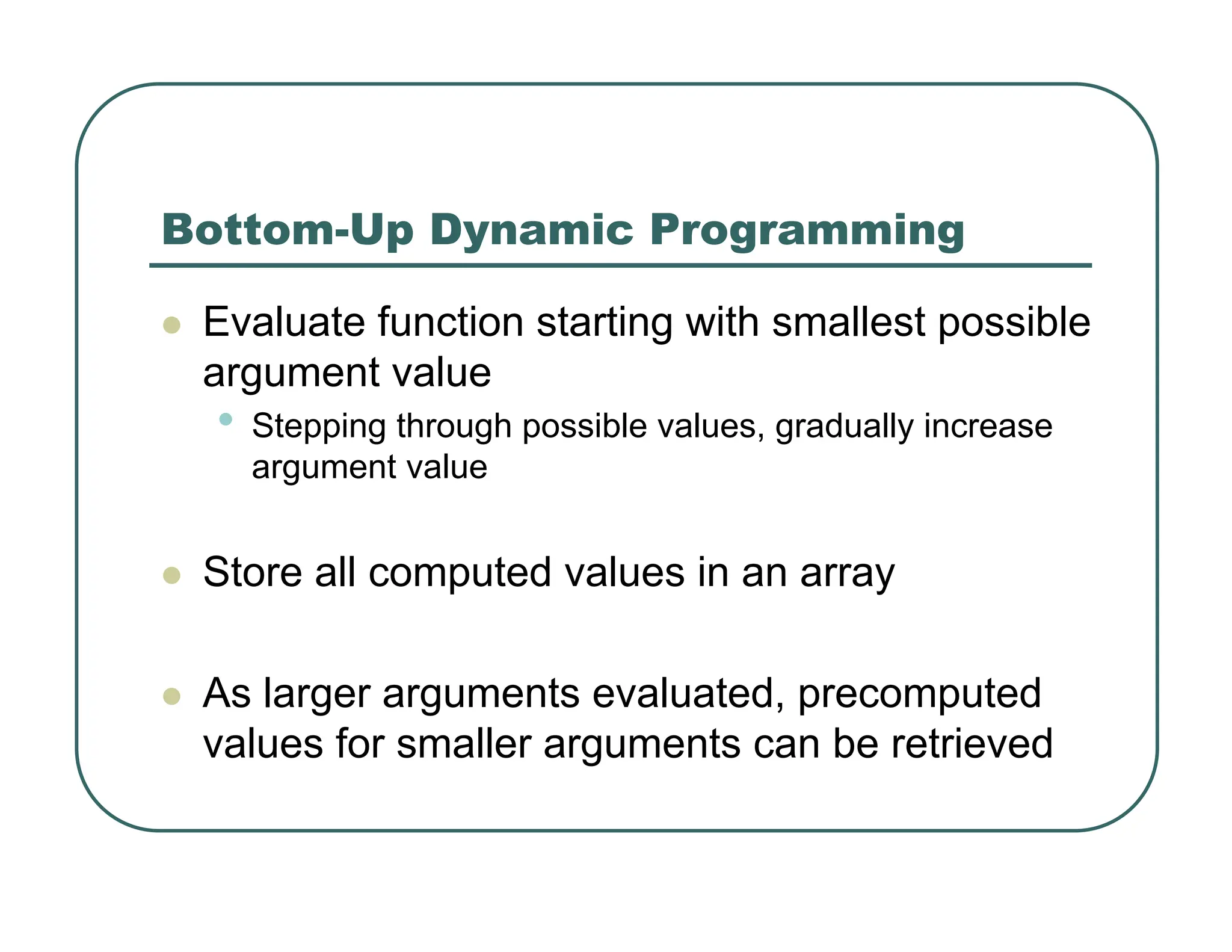
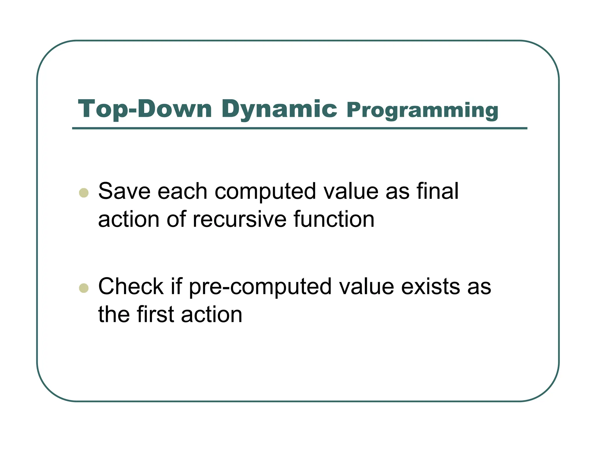
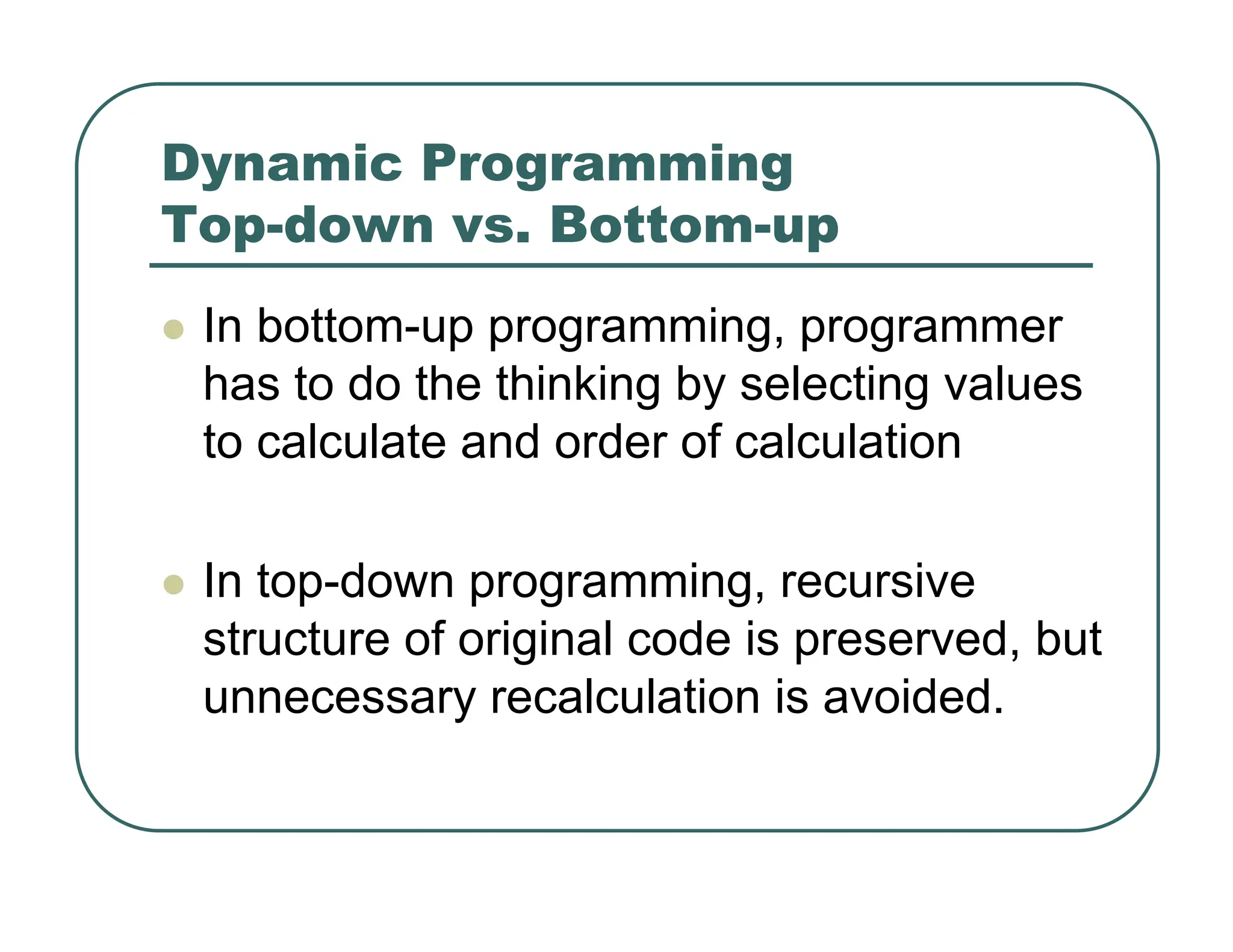
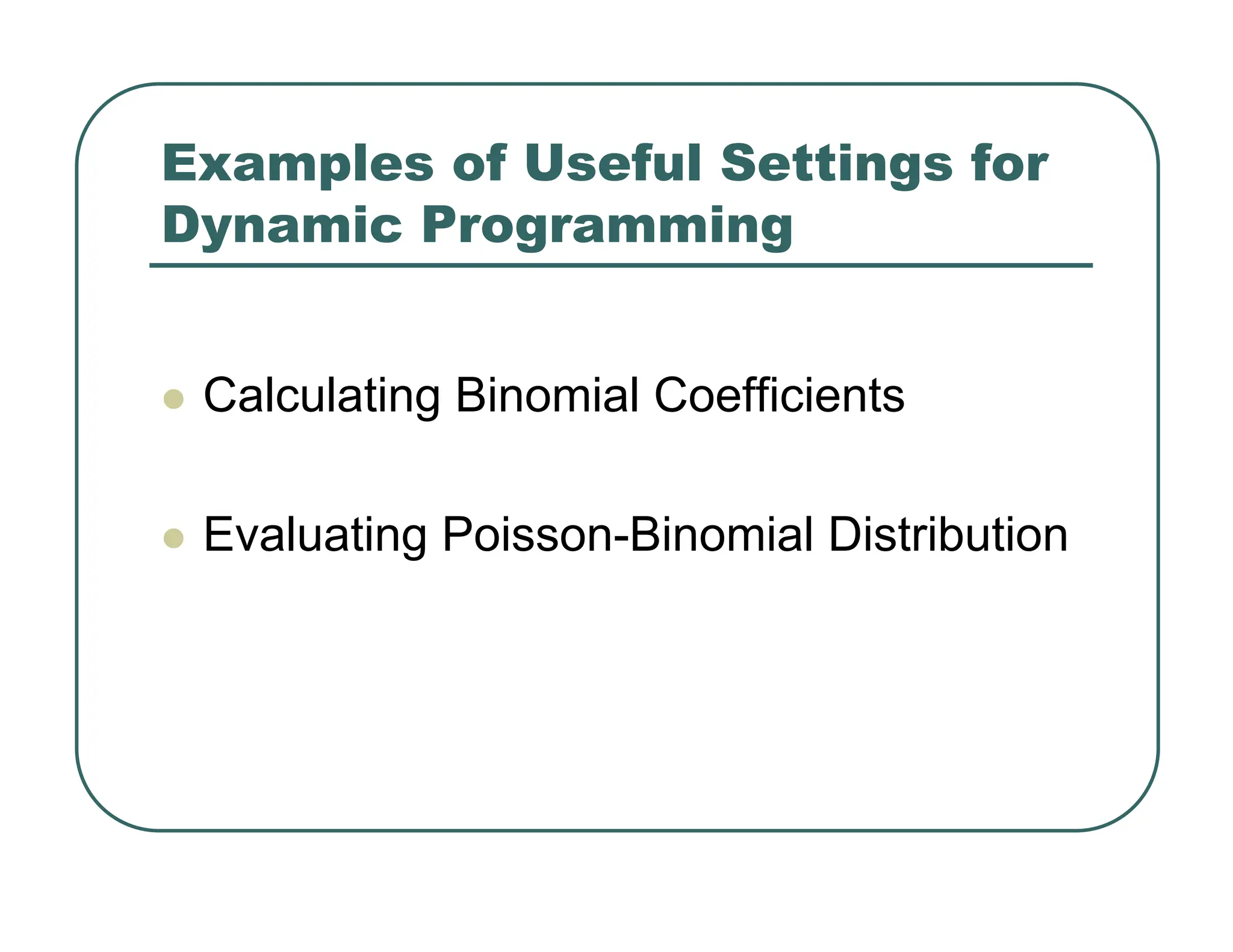
Recursive functions can be used to solve problems by breaking them down into smaller subproblems. Dynamic programming is a technique for solving recursive problems more efficiently by avoiding recomputing results. It works by either building up the solution from smallest to largest subproblems (bottom-up) or saving computed results to lookup later (top-down). Examples where dynamic programming improves performance include calculating factorials, Fibonacci numbers, binomial coefficients, and the Poisson-binomial distribution.

![Question 2
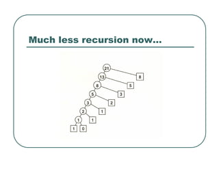
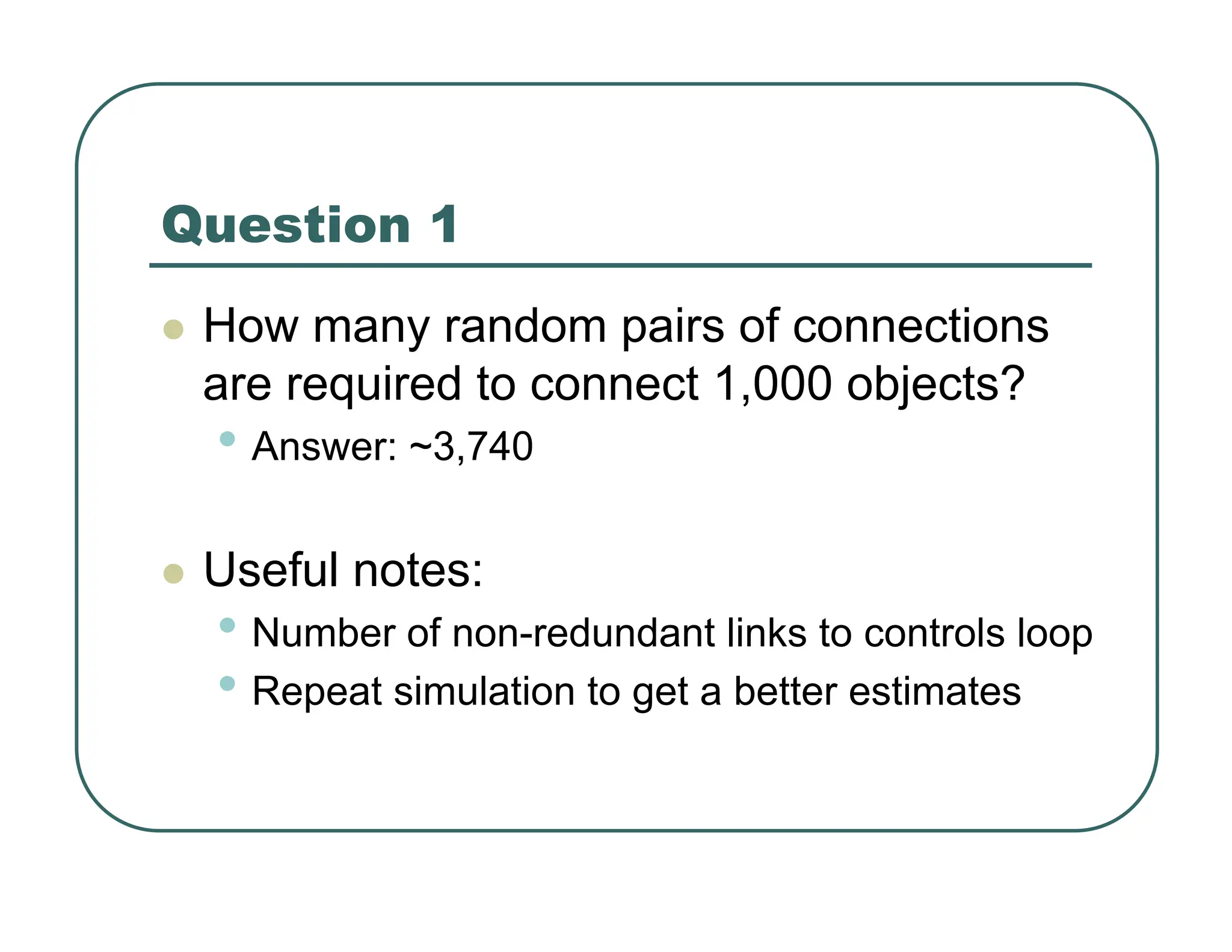
z Path lengths in the saturated tree…
• ~1.8 nodes on average
• ~5 nodes for maximum path
z Random data is far from worst case
• Worst case would be paths of log2 N nodes
z Path lengths can be calculated using weights[]](https://image.slidesharecdn.com/815-240316120018-c1feb61a/85/815-07-machine-learning-using-python-pdf-4-320.jpg)

![Recursive Binary Search
int search(int a[], int value, int start, int stop)
{
// Search failed
if (start > stop)
return -1;
// Find midpoint
int mid = (start + stop) / 2;
// Compare midpoint to value
if (value == a[mid]) return mid;
// Reduce input in half!!!
if (value < a[mid])
return search(a, start, mid – 1 };
else
return search(a, mid + 1, stop);
}](https://image.slidesharecdn.com/815-240316120018-c1feb61a/85/815-07-machine-learning-using-python-pdf-17-320.jpg)
![Recursive Maximum
int Maximum(int a[], int start, int stop)
{
int left, right;
// Maximum of one element
if (start == stop)
return a[start];
left = Maximum(a, start, (start + stop) / 2);
right = Maximum(a, (start + stop) / 2 + 1, stop);
// Reduce input in half!!!
if (left > right)
return left;
else
return right;
}](https://image.slidesharecdn.com/815-240316120018-c1feb61a/85/815-07-machine-learning-using-python-pdf-18-320.jpg)


![Fibonacci Numbers in C
int Fibonacci(int i)
{
int fib[LARGE_NUMBER], j;
fib[0] = 0;
fib[1] = 1;
for (j = 2; j <= i; j++)
fib[j] = fib[j – 1] + fib[j – 2];
return fib[i];
}](https://image.slidesharecdn.com/815-240316120018-c1feb61a/85/815-07-machine-learning-using-python-pdf-26-320.jpg)
![Fibonacci With Dynamic Memory
int Fibonacci(int i)
{
int * fib, j, result;
if (i < 2) return i;
fib = malloc(sizeof(int) * (i + 1));
fib[0] = 0; fib[1] = 1;
for (j = 2; j <= i; j++)
fib[j] = fib[j – 1] + fib[j – 2];
result = fib[i];
free(fib);
return result;
}](https://image.slidesharecdn.com/815-240316120018-c1feb61a/85/815-07-machine-learning-using-python-pdf-27-320.jpg)
![Fibonacci Numbers in R
Fibonacci <- function(i)
{
if (i < 2)
return(i)
// Arrays in R are zero based, so ensure i >= 1
i <- i + 1
fib <- rep(0, i)
fib[1] <- 0;
fib[2] <- 1;
for (j in seq(3,i))
fib[j] <- fib[j – 1] + fib[j – 2]
return (fib[i])
}](https://image.slidesharecdn.com/815-240316120018-c1feb61a/85/815-07-machine-learning-using-python-pdf-28-320.jpg)
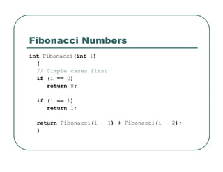
![Fibonacci Numbers
int Fibonacci(int i)
{
// Simple cases first
if (saveF[i] > 0)
return saveF[i];
if (i <= 1)
return i;
// Recursion
saveF[i] = Fibonacci(i – 1) + Fibonacci(i – 2);
return saveF[i];
}](https://image.slidesharecdn.com/815-240316120018-c1feb61a/85/815-07-machine-learning-using-python-pdf-30-320.jpg)
![Fibonacci Numbers
Fibonacci <- function(i)
{
# Simple cases first
if (i <= 1)
return (i)
if (saveF[i] > 0)
return (saveF[i])
# Recursion
saveF[i] <<- Fibonacci(i – 1) + Fibonacci(i – 2)
return (saveF[i])
}](https://image.slidesharecdn.com/815-240316120018-c1feb61a/85/815-07-machine-learning-using-python-pdf-32-320.jpg)

![Implementation in R
Choose <- function(N, k)
{
M <- matrix(nrow = N, ncol = N + 1)
for (i in 1:N)
{
M[i,1] <- M[i, i + 1] <- 1
if (i > 1)
for (j in 2:i)
M[i,j] <- M[i - 1, j - 1] + M[i - 1, j];
}
return(M[N,k + 1])
}](https://image.slidesharecdn.com/815-240316120018-c1feb61a/85/815-07-machine-learning-using-python-pdf-37-320.jpg)
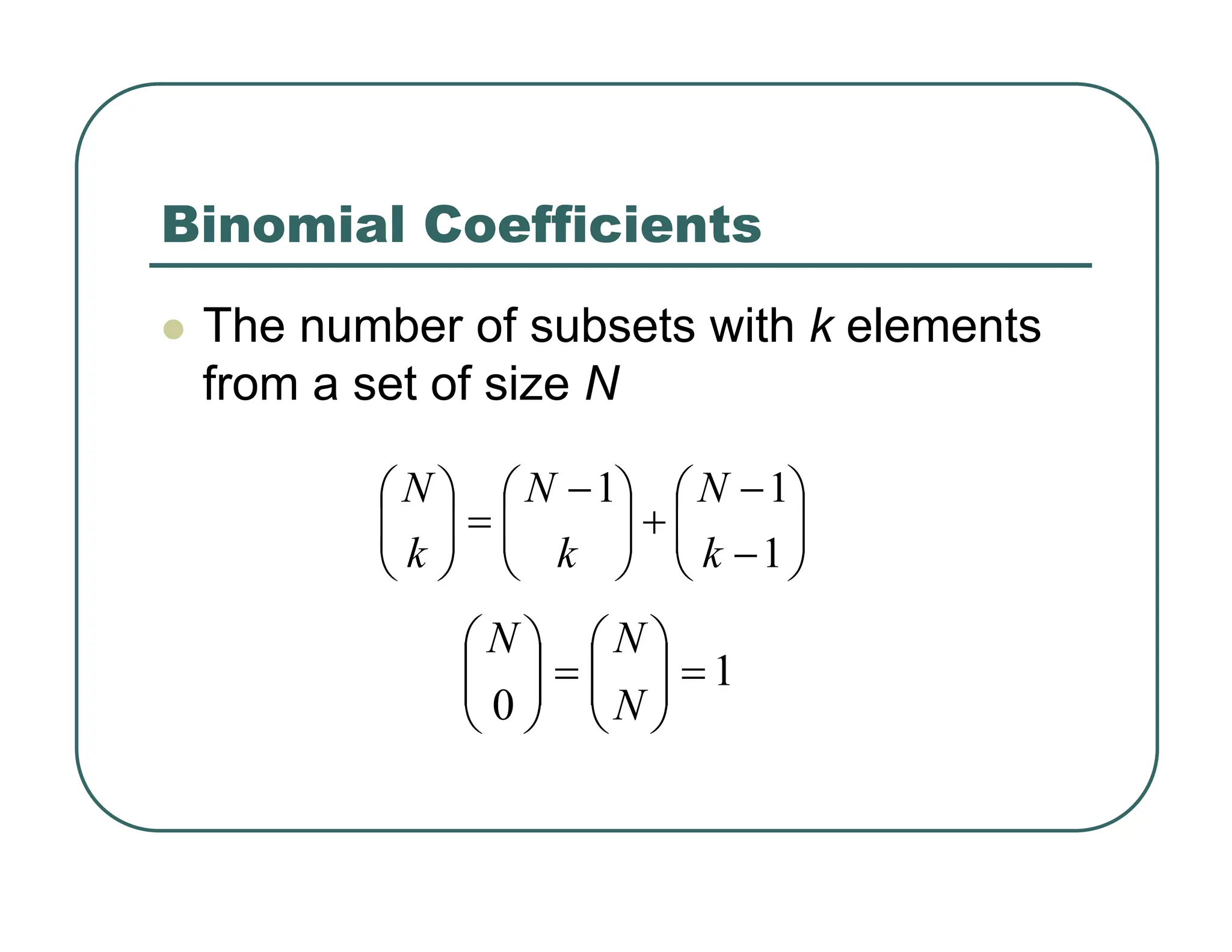
![Implementation in C
int Choose(int N, int k)
{
int i, j, M[MAX_N][MAX_N];
for (i = 1; i <= N; i++)
{
M[i][0] = M[i][i] = 1;
for (j = 1; j < i; j++)
M[i][j] = M[i - 1][j - 1] + M[i - 1][j];
}
return M[N][k];
}](https://image.slidesharecdn.com/815-240316120018-c1feb61a/85/815-07-machine-learning-using-python-pdf-38-320.jpg)

![Question 2
z Path lengths in the saturated tree…
• ~1.8 nodes on average
• ~5 nodes for maximum path
z Random data is far from worst case
• Worst case would be paths of log2 N nodes
z Path lengths can be calculated using weights[]](https://image.slidesharecdn.com/815-240316120018-c1feb61a/75/815-07-machine-learning-using-python-pdf-4-2048.jpg)


![Recursive Binary Search
int search(int a[], int value, int start, int stop)
{
// Search failed
if (start > stop)
return -1;
// Find midpoint
int mid = (start + stop) / 2;
// Compare midpoint to value
if (value == a[mid]) return mid;
// Reduce input in half!!!
if (value < a[mid])
return search(a, start, mid – 1 };
else
return search(a, mid + 1, stop);
}](https://image.slidesharecdn.com/815-240316120018-c1feb61a/75/815-07-machine-learning-using-python-pdf-17-2048.jpg)
![Recursive Maximum
int Maximum(int a[], int start, int stop)
{
int left, right;
// Maximum of one element
if (start == stop)
return a[start];
left = Maximum(a, start, (start + stop) / 2);
right = Maximum(a, (start + stop) / 2 + 1, stop);
// Reduce input in half!!!
if (left > right)
return left;
else
return right;
}](https://image.slidesharecdn.com/815-240316120018-c1feb61a/75/815-07-machine-learning-using-python-pdf-18-2048.jpg)


![Fibonacci Numbers in C
int Fibonacci(int i)
{
int fib[LARGE_NUMBER], j;
fib[0] = 0;
fib[1] = 1;
for (j = 2; j <= i; j++)
fib[j] = fib[j – 1] + fib[j – 2];
return fib[i];
}](https://image.slidesharecdn.com/815-240316120018-c1feb61a/75/815-07-machine-learning-using-python-pdf-26-2048.jpg)
![Fibonacci With Dynamic Memory
int Fibonacci(int i)
{
int * fib, j, result;
if (i < 2) return i;
fib = malloc(sizeof(int) * (i + 1));
fib[0] = 0; fib[1] = 1;
for (j = 2; j <= i; j++)
fib[j] = fib[j – 1] + fib[j – 2];
result = fib[i];
free(fib);
return result;
}](https://image.slidesharecdn.com/815-240316120018-c1feb61a/75/815-07-machine-learning-using-python-pdf-27-2048.jpg)
![Fibonacci Numbers in R
Fibonacci <- function(i)
{
if (i < 2)
return(i)
// Arrays in R are zero based, so ensure i >= 1
i <- i + 1
fib <- rep(0, i)
fib[1] <- 0;
fib[2] <- 1;
for (j in seq(3,i))
fib[j] <- fib[j – 1] + fib[j – 2]
return (fib[i])
}](https://image.slidesharecdn.com/815-240316120018-c1feb61a/75/815-07-machine-learning-using-python-pdf-28-2048.jpg)
![Fibonacci Numbers
int Fibonacci(int i)
{
// Simple cases first
if (saveF[i] > 0)
return saveF[i];
if (i <= 1)
return i;
// Recursion
saveF[i] = Fibonacci(i – 1) + Fibonacci(i – 2);
return saveF[i];
}](https://image.slidesharecdn.com/815-240316120018-c1feb61a/75/815-07-machine-learning-using-python-pdf-30-2048.jpg)
![Fibonacci Numbers
Fibonacci <- function(i)
{
# Simple cases first
if (i <= 1)
return (i)
if (saveF[i] > 0)
return (saveF[i])
# Recursion
saveF[i] <<- Fibonacci(i – 1) + Fibonacci(i – 2)
return (saveF[i])
}](https://image.slidesharecdn.com/815-240316120018-c1feb61a/75/815-07-machine-learning-using-python-pdf-32-2048.jpg)

![Implementation in R
Choose <- function(N, k)
{
M <- matrix(nrow = N, ncol = N + 1)
for (i in 1:N)
{
M[i,1] <- M[i, i + 1] <- 1
if (i > 1)
for (j in 2:i)
M[i,j] <- M[i - 1, j - 1] + M[i - 1, j];
}
return(M[N,k + 1])
}](https://image.slidesharecdn.com/815-240316120018-c1feb61a/75/815-07-machine-learning-using-python-pdf-37-2048.jpg)
![Implementation in C
int Choose(int N, int k)
{
int i, j, M[MAX_N][MAX_N];
for (i = 1; i <= N; i++)
{
M[i][0] = M[i][i] = 1;
for (j = 1; j < i; j++)
M[i][j] = M[i - 1][j - 1] + M[i - 1][j];
}
return M[N][k];
}](https://image.slidesharecdn.com/815-240316120018-c1feb61a/75/815-07-machine-learning-using-python-pdf-38-2048.jpg)