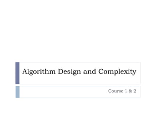

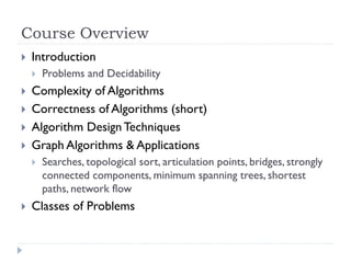

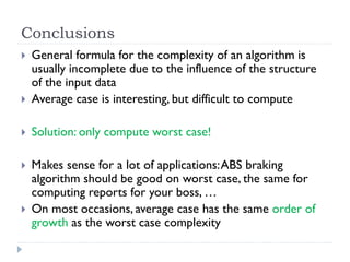
![Problems and Algorithms
Problems 1 – n Algorithms
Problem: Sorting
1+ algorithms to solve each problem
An algorithm usually solves only 1 problem
Given an array with n numbers A[n], arrange the elements in
the array such that any two consecutive elements are sorted
(A[i] <= A[i + 1] for i = 1..n-1)
Arrays A[1..n]
Algorithms:
Quick Sort, Merge Sort, Heap Sort, Bubble Sort, Insertion Sort,
Selection Sort, Radix Sort, Bucket Sort, …](https://image.slidesharecdn.com/adc12-101021042844-phpapp01/85/Algorithm-Design-and-Complexity-Course-1-2-9-320.jpg)


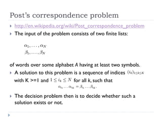

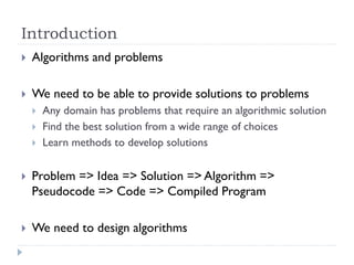
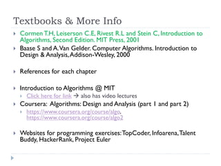
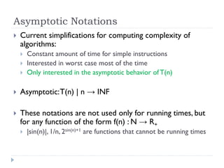
![Running Time
Measure of the time complexity of an algorithm
It is a theoretical measure that is dependent of the input
data and the processing performed by an algorithm
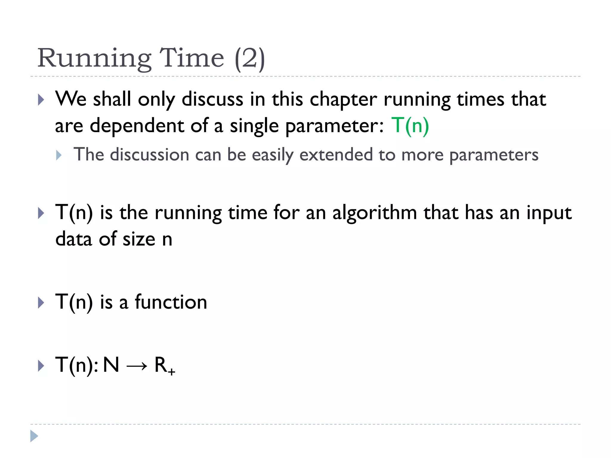
We define the running time as a function that only
depends on the size of the input data
The size of the input data is measured by positive integers
For arrays: A[n]
For graphs: G(V, E), |V| = n, |E| = m
For multiplying 3 matrices: lines1, columns1, columns2](https://image.slidesharecdn.com/adc12-101021042844-phpapp01/85/Algorithm-Design-and-Complexity-Course-1-2-24-320.jpg)
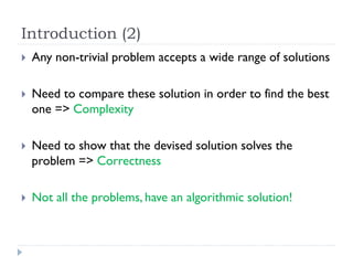
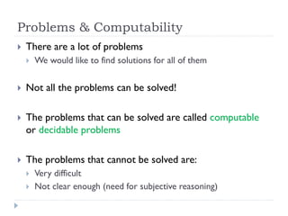
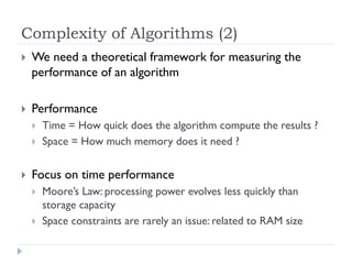
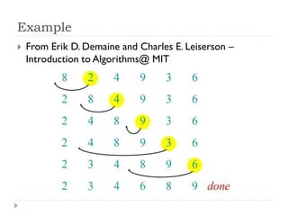
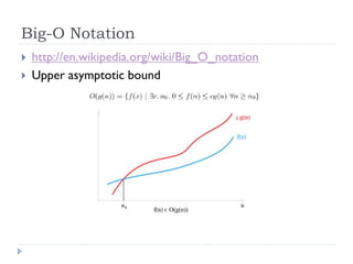
![Example – Insertion Sort
http://en.wikipedia.org/wiki/Insertion_sort
Problem: Sorting an array A[n]
Solution: Insertion sort
Every repetition of the main loop of insertion sort
removes an element from the input data, inserting it into
the correct position in the already-sorted list, until no
input elements remain.
The already-sorted list is the sub-array on the left side
Usually, the removed element is the next one](https://image.slidesharecdn.com/adc12-101021042844-phpapp01/85/Algorithm-Design-and-Complexity-Course-1-2-26-320.jpg)
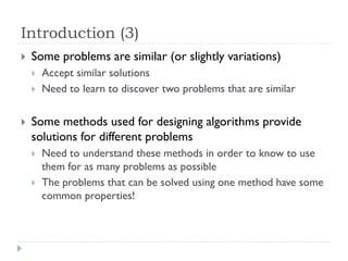
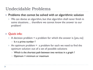
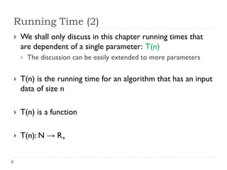
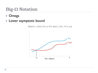
![Insertion Sort - Pseudocode
InsertionSort( A[1..n] )
1. FOR (j = 2 .. n)
2.
x = A[j]
3.
i=j–1
4.
5.
6.
7.
8.
// element to be inserted
// position on the right side of
//
the sorted sub-array
WHILE (i > 0 AND x < A[i]) // while not in position
A[i + 1] = A[i]
// move to right
i-// continue
A[i + 1] = x
RETURN A](https://image.slidesharecdn.com/adc12-101021042844-phpapp01/85/Algorithm-Design-and-Complexity-Course-1-2-27-320.jpg)
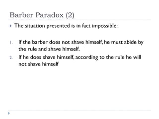
![Worst Case Complexity
Happens when the array is sorted descending
In this case, all the elements x = A[j] are lower than all
the previous elements
Therefore, they must be moved to the beginning of the
array
Thus:
tj = j (from j – 1 to 0)
T1 = (j=2..n) j = n*(n+1) / 2 – 1
T2 = (j=2..n) (j - 1) = n*(n-1) / 2
Tworst(n) = a*n2 + b*n + c
quadratic time](https://image.slidesharecdn.com/adc12-101021042844-phpapp01/85/Algorithm-Design-and-Complexity-Course-1-2-32-320.jpg)
![Best Case Complexity
Happens when the array is sorted ascending
In this case, all the elements x = A[j] are higher than all
the previous elements
Therefore, they are not moved
Thus:
tj = 1
T1 = (j=2..n) 1 = n-1
T2 = (j=2..n) (1 - 1) = 0
Tbest(n) = b1*n + c1
linear time](https://image.slidesharecdn.com/adc12-101021042844-phpapp01/85/Algorithm-Design-and-Complexity-Course-1-2-33-320.jpg)
![Average Case Complexity
It is interesting to compute it precisely
It is very difficult to compute it precisely!
Should take into consideration the distribution of the input
data and sum up over all possible instances of the input data
averaged by their distribution
See example of formula in blackboard
Not feasible
Simpler solution: on average, an element x = A[j] in inserted in
the middle of the already-sorted list
Recompute T1 and T2 for this case => still a quadratic solution](https://image.slidesharecdn.com/adc12-101021042844-phpapp01/85/Algorithm-Design-and-Complexity-Course-1-2-34-320.jpg)


![Exercises – Set 1
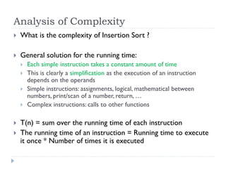
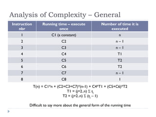
What is the complexity of the following algorithms ?
Matrix_add_1 (A[n][n],B[n][n]) {
for (i = 1,n) {
for (j = 1,n) {
C[i][j] = 0
}
}
for (i = 1,n) {
for (j = 1,n) {
C[i][j] = A[i][j] + B[i][j]
}
}
return C
}](https://image.slidesharecdn.com/adc12-101021042844-phpapp01/85/Algorithm-Design-and-Complexity-Course-1-2-46-320.jpg)
![Matrix_add_2 (A[n][n],B[n][n]) {
for (i = 1,n) {
for (j = 1,n) {
B[i][j] = A[i][j] + B[i][j]
}
}
return B
}](https://image.slidesharecdn.com/adc12-101021042844-phpapp01/85/Algorithm-Design-and-Complexity-Course-1-2-47-320.jpg)
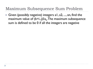
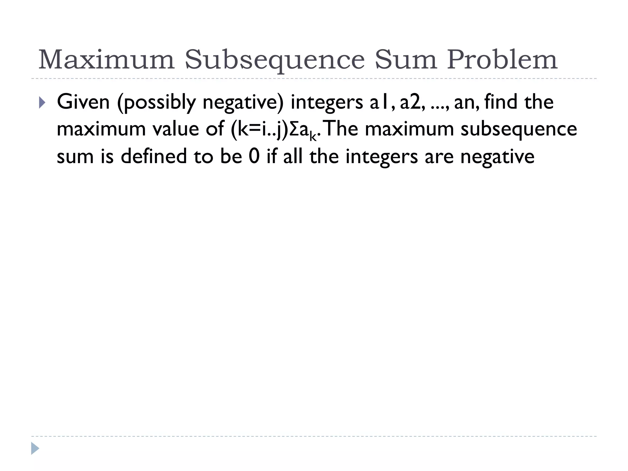
![Let A[1] … A[N] be an array of integers that contains a
sequence of length N.
Let sum and maxSum be integers initialized to 0.
For integer i = 1 to N do
Let sum = 0
For integer j = i to N do
Let sum = sum + A[ j ]
If( sum > maxSum ) then
Let maxSum = sum
Return maxSum](https://image.slidesharecdn.com/adc12-101021042844-phpapp01/85/Algorithm-Design-and-Complexity-Course-1-2-49-320.jpg)


![Problems and Algorithms
Problems 1 – n Algorithms
Problem: Sorting
1+ algorithms to solve each problem
An algorithm usually solves only 1 problem
Given an array with n numbers A[n], arrange the elements in
the array such that any two consecutive elements are sorted
(A[i] <= A[i + 1] for i = 1..n-1)
Arrays A[1..n]
Algorithms:
Quick Sort, Merge Sort, Heap Sort, Bubble Sort, Insertion Sort,
Selection Sort, Radix Sort, Bucket Sort, …](https://image.slidesharecdn.com/adc12-101021042844-phpapp01/75/Algorithm-Design-and-Complexity-Course-1-2-9-2048.jpg)


![Running Time
Measure of the time complexity of an algorithm
It is a theoretical measure that is dependent of the input
data and the processing performed by an algorithm
We define the running time as a function that only
depends on the size of the input data
The size of the input data is measured by positive integers
For arrays: A[n]
For graphs: G(V, E), |V| = n, |E| = m
For multiplying 3 matrices: lines1, columns1, columns2](https://image.slidesharecdn.com/adc12-101021042844-phpapp01/75/Algorithm-Design-and-Complexity-Course-1-2-24-2048.jpg)
![Example – Insertion Sort
http://en.wikipedia.org/wiki/Insertion_sort
Problem: Sorting an array A[n]
Solution: Insertion sort
Every repetition of the main loop of insertion sort
removes an element from the input data, inserting it into
the correct position in the already-sorted list, until no
input elements remain.
The already-sorted list is the sub-array on the left side
Usually, the removed element is the next one](https://image.slidesharecdn.com/adc12-101021042844-phpapp01/75/Algorithm-Design-and-Complexity-Course-1-2-26-2048.jpg)
![Insertion Sort - Pseudocode
InsertionSort( A[1..n] )
1. FOR (j = 2 .. n)
2.
x = A[j]
3.
i=j–1
4.
5.
6.
7.
8.
// element to be inserted
// position on the right side of
//
the sorted sub-array
WHILE (i > 0 AND x < A[i]) // while not in position
A[i + 1] = A[i]
// move to right
i-// continue
A[i + 1] = x
RETURN A](https://image.slidesharecdn.com/adc12-101021042844-phpapp01/75/Algorithm-Design-and-Complexity-Course-1-2-27-2048.jpg)


![Worst Case Complexity
Happens when the array is sorted descending
In this case, all the elements x = A[j] are lower than all
the previous elements
Therefore, they must be moved to the beginning of the
array
Thus:
tj = j (from j – 1 to 0)
T1 = (j=2..n) j = n*(n+1) / 2 – 1
T2 = (j=2..n) (j - 1) = n*(n-1) / 2
Tworst(n) = a*n2 + b*n + c
quadratic time](https://image.slidesharecdn.com/adc12-101021042844-phpapp01/75/Algorithm-Design-and-Complexity-Course-1-2-32-2048.jpg)
![Best Case Complexity
Happens when the array is sorted ascending
In this case, all the elements x = A[j] are higher than all
the previous elements
Therefore, they are not moved
Thus:
tj = 1
T1 = (j=2..n) 1 = n-1
T2 = (j=2..n) (1 - 1) = 0
Tbest(n) = b1*n + c1
linear time](https://image.slidesharecdn.com/adc12-101021042844-phpapp01/75/Algorithm-Design-and-Complexity-Course-1-2-33-2048.jpg)
![Average Case Complexity
It is interesting to compute it precisely
It is very difficult to compute it precisely!
Should take into consideration the distribution of the input
data and sum up over all possible instances of the input data
averaged by their distribution
See example of formula in blackboard
Not feasible
Simpler solution: on average, an element x = A[j] in inserted in
the middle of the already-sorted list
Recompute T1 and T2 for this case => still a quadratic solution](https://image.slidesharecdn.com/adc12-101021042844-phpapp01/75/Algorithm-Design-and-Complexity-Course-1-2-34-2048.jpg)


![Exercises – Set 1
What is the complexity of the following algorithms ?
Matrix_add_1 (A[n][n],B[n][n]) {
for (i = 1,n) {
for (j = 1,n) {
C[i][j] = 0
}
}
for (i = 1,n) {
for (j = 1,n) {
C[i][j] = A[i][j] + B[i][j]
}
}
return C
}](https://image.slidesharecdn.com/adc12-101021042844-phpapp01/75/Algorithm-Design-and-Complexity-Course-1-2-46-2048.jpg)
![Matrix_add_2 (A[n][n],B[n][n]) {
for (i = 1,n) {
for (j = 1,n) {
B[i][j] = A[i][j] + B[i][j]
}
}
return B
}](https://image.slidesharecdn.com/adc12-101021042844-phpapp01/75/Algorithm-Design-and-Complexity-Course-1-2-47-2048.jpg)
![Let A[1] … A[N] be an array of integers that contains a
sequence of length N.
Let sum and maxSum be integers initialized to 0.
For integer i = 1 to N do
Let sum = 0
For integer j = i to N do
Let sum = sum + A[ j ]
If( sum > maxSum ) then
Let maxSum = sum
Return maxSum](https://image.slidesharecdn.com/adc12-101021042844-phpapp01/75/Algorithm-Design-and-Complexity-Course-1-2-49-2048.jpg)

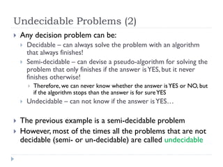
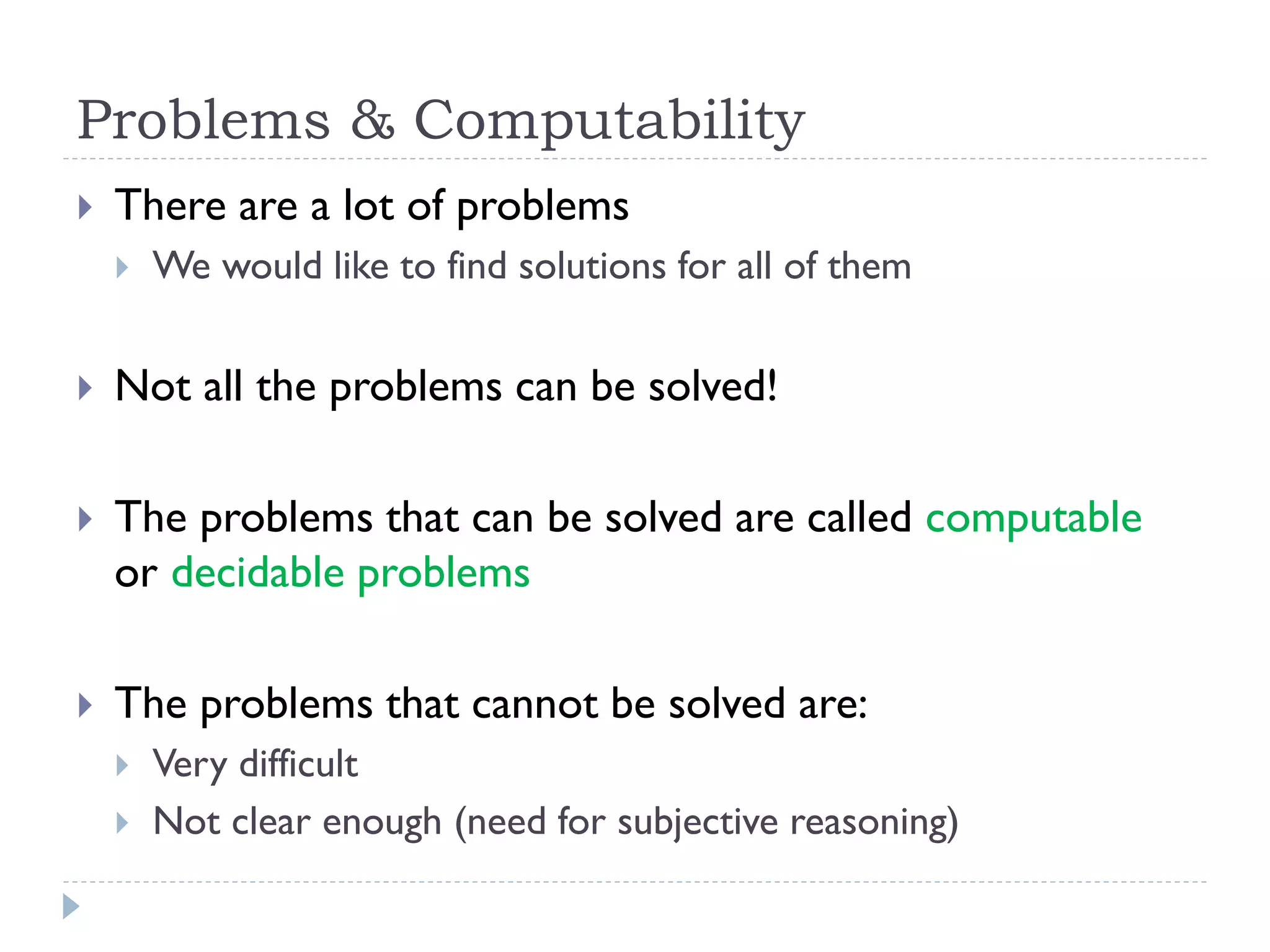
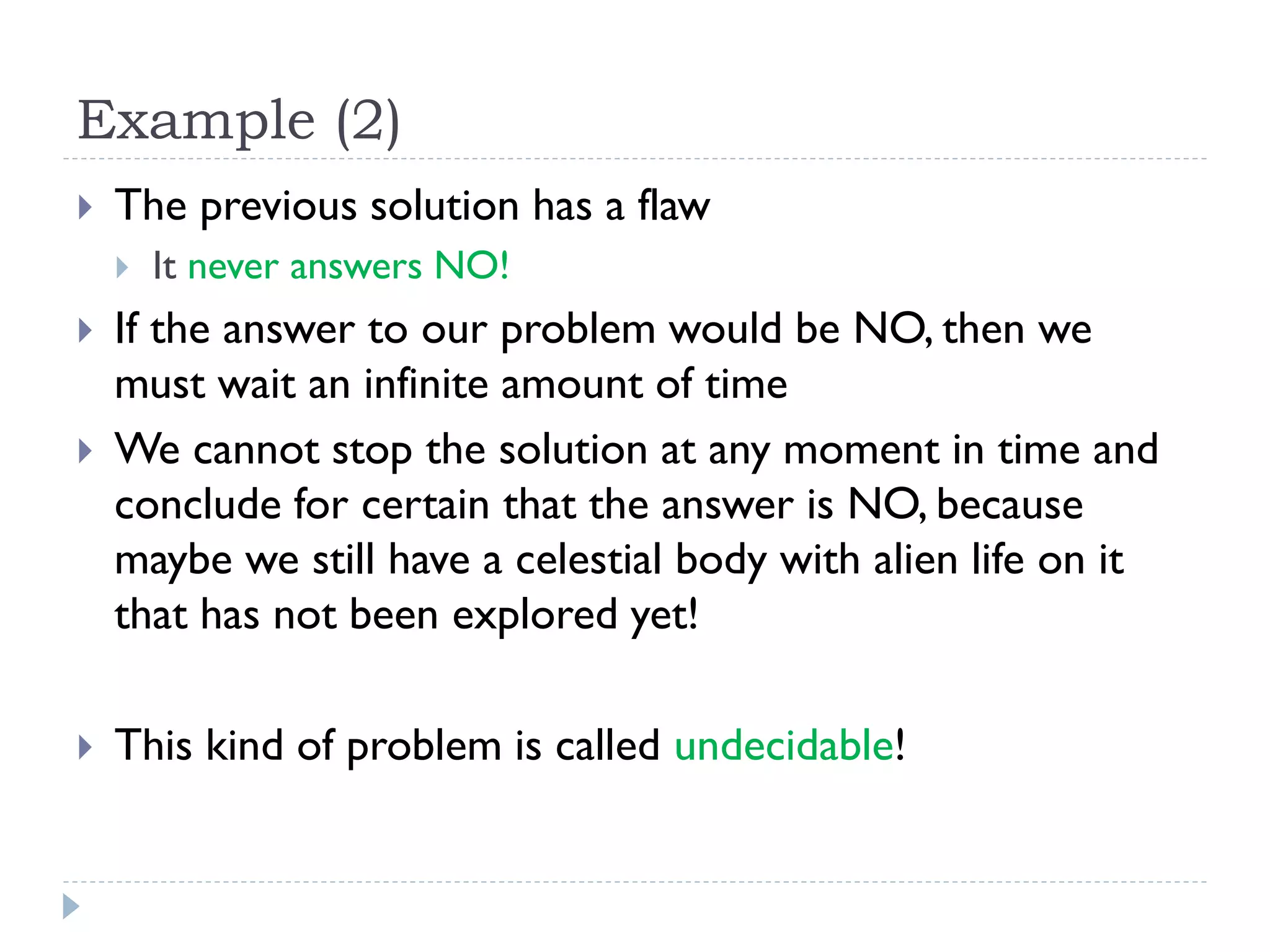
This document outlines a course on algorithm design and complexity, emphasizing the need to find the best algorithmic solutions to problems while evaluating the correctness and complexity of those solutions. It highlights different types of problems, including decidable and undecidable ones, and discusses algorithm performance and efficiency through measures like time and space complexity. The document also includes course information, grading criteria, and various references for further study.


