Downloaded 1,230 times


![Tutorial 1: Simulating Flow in a Static Mixer Using CFX in Standalone Mode: Defining a Simulation in ANSYS CFX-Pre
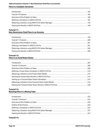
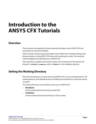
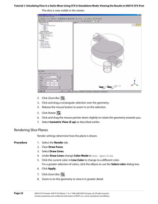
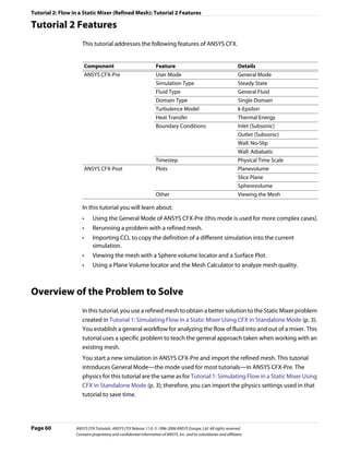
Defining Model Data
You need to define the type of flow and the physical models to use in the fluid domain.
You will specify the flow as steady state with turbulence and heat transfer. Turbulence is
modeled using the k - ε turbulence model and heat transfer using the thermal energy
model. The k - ε turbulence model is a commonly used model and is suitable for a wide
range of applications. The thermal energy model neglects high speed energy effects and is
therefore suitable for low speed flow applications.
Procedure 1. Ensure that Physics Definition is displayed.
2. Under Model Data, set Reference Pressure to 1 [atm].
All other pressure settings are relative to this reference pressure.
3. Set Heat Transfer to Thermal Energy.
4. Set Turbulence to k-Epsilon.
5. Click Next.
Defining Boundaries
The CFD model requires the definition of conditions on the boundaries of the domain.
Procedure 1. Ensure that Boundary Definition is displayed.
2. Delete Inlet and Outlet from the list by right-clicking each and selecting Delete.
3. Right-click in the blank area where Inlet and Outlet were listed, then select New.
4. Set Name to in1.
5. Click OK.
The boundary is created and, when selected, properties related to the boundary are
displayed.
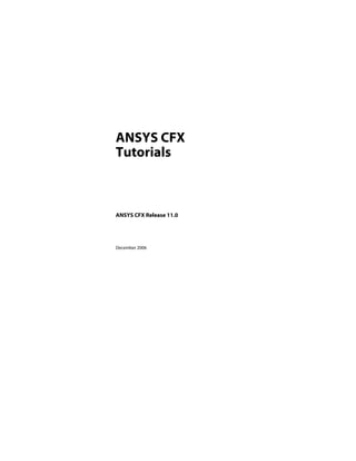
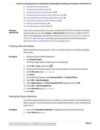
Setting Boundary Data
Once boundaries are created, you need to create associated data. Based on Figure 1, you will
define the first inlet boundary condition’s velocity and temperature.
Procedure 1. Ensure that Boundary Data is displayed.
2. Set Boundary Type to Inlet.
3. Set Location to in1.
Setting Flow Specification
Once boundary data is defined, the boundary needs to have the flow specification assigned.
Procedure 1. Ensure that Flow Specification is displayed.
2. Set Option to Normal Speed.
3. Set Normal Speed to 2 [m s^-1].
ANSYS CFX Tutorials. ANSYS CFX Release 11.0. © 1996-2006 ANSYS Europe, Ltd. All rights reserved. Page 9
Contains proprietary and confidential information of ANSYS, Inc. and its subsidiaries and affiliates.](https://image.slidesharecdn.com/ansys11tutorial-111218135319-phpapp01/85/Ansys-11-tutorial-21-320.jpg)
![Tutorial 1: Simulating Flow in a Static Mixer Using CFX in Standalone Mode: Defining a Simulation in ANSYS CFX-Pre
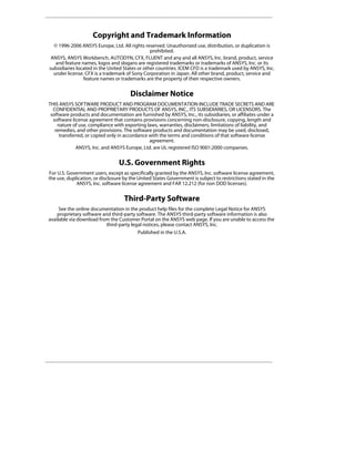
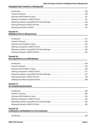
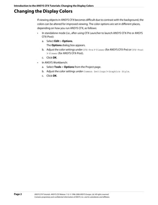
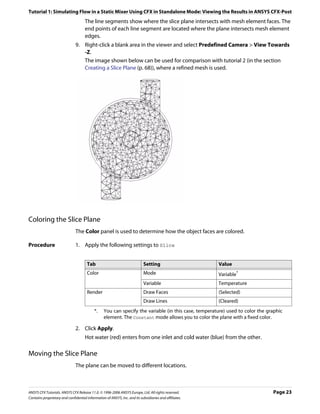
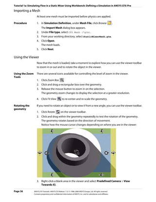
Setting Temperature Specification
Once flow specification is defined, the boundary needs to have temperature assigned.
Procedure 1. Ensure that Temperature Specification is displayed.
2. Set Static Temperature to 315 [K].
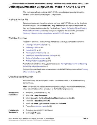
Reviewing the Boundary Condition Definitions
Defining the boundary condition for in1 required several steps. Here the settings are
reviewed for accuracy.
Based on Figure 1, the first inlet boundary condition consists of a velocity of 2 m/s and a
temperature of 315 K at one of the side inlets.
Procedure 1. Review the boundary in1 settings for accuracy. They should be as follows:
Tab Setting Value
Boundary Data Boundary Type Inlet
Location in1
Flow Specification Option Normal Speed
Normal Speed 2 [m s^-1]
Temperature Specification Static Temperature 315 [K]
Creating the Second Inlet Boundary Definition
Based on Figure 1, you know the second inlet boundary condition consists of a velocity of 2
m/s and a temperature of 285 K at one of the side inlets. You will define that now.
Procedure 1. Under Boundary Definition, right-click in the selector area and select New.
2. Create a new boundary named in2 with these settings:
Tab Setting Value
Boundary Data Boundary Type Inlet
Location in2
Flow Specification Option Normal Speed
Normal Speed 2 [m s^-1]
Temperature Specification Static Temperature 285 [K]
Creating the Outlet Boundary Definition
Now that the second inlet boundary has been created, the same concepts can be applied to
building the outlet boundary.
1. Create a new boundary named out with these settings:
Page 10 ANSYS CFX Tutorials. ANSYS CFX Release 11.0. © 1996-2006 ANSYS Europe, Ltd. All rights reserved.
Contains proprietary and confidential information of ANSYS, Inc. and its subsidiaries and affiliates.](https://image.slidesharecdn.com/ansys11tutorial-111218135319-phpapp01/85/Ansys-11-tutorial-22-320.jpg)
![Tutorial 1: Simulating Flow in a Static Mixer Using CFX in Standalone Mode: Defining a Simulation in ANSYS CFX-Pre
Tab Setting Value
Boundary Data Boundary Type Outlet
Location out
Flow Specification Option Average Static Pressure
Relative Pressure 0 [Pa]
2. Click Next.
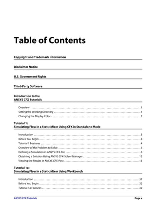
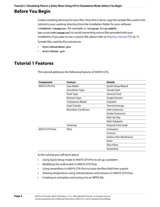
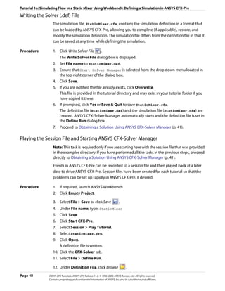
Moving to General Mode
There are no further boundary conditions that need to be set. All 2D exterior regions that
have not been assigned to a boundary condition are automatically assigned to the default
boundary condition.
Procedure 1. Set Operation to Enter General Mode and click Finish.
The three boundary conditions are displayed in the viewer as sets of arrows at the
boundary surfaces. Inlet boundary arrows are directed into the domain. Outlet
boundary arrows are directed out of the domain.
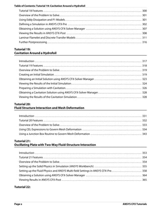
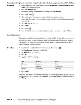
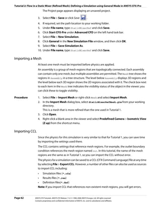
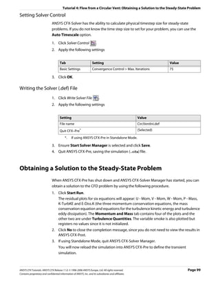
Setting Solver Control
Solver Control parameters control aspects of the numerical solution generation process.
While an upwind advection scheme is less accurate than other advection schemes, it is also
more robust. This advection scheme is suitable for obtaining an initial set of results, but in
general should not be used to obtain final accurate results.
The time scale can be calculated automatically by the solver or set manually. The Automatic
option tends to be conservative, leading to reliable, but often slow, convergence. It is often
possible to accelerate convergence by applying a time scale factor or by choosing a manual
value that is more aggressive than the Automatic option. In this tutorial, you will select a
physical time scale, leading to convergence that is twice as fast as the Automatic option.
Procedure 1. Click Solver Control .
2. On the Basic Settings tab, set Advection Scheme > Option to Upwind.
3. Set Convergence Control > Fluid Timescale Control > Timescale Control to
Physical Timescale and set the physical timescale value to 2 [s].
4. Click OK.
Writing the Solver (.def) File
The simulation file, StaticMixer.cfx, contains the simulation definition in a format that
can be loaded by ANSYS CFX-Pre, allowing you to complete (if applicable), restore, and
modify the simulation definition. The simulation file differs from the definition file in that it
can be saved at any time while defining the simulation.
Procedure 1. Click Write Solver File .
ANSYS CFX Tutorials. ANSYS CFX Release 11.0. © 1996-2006 ANSYS Europe, Ltd. All rights reserved. Page 11
Contains proprietary and confidential information of ANSYS, Inc. and its subsidiaries and affiliates.](https://image.slidesharecdn.com/ansys11tutorial-111218135319-phpapp01/85/Ansys-11-tutorial-23-320.jpg)
![Tutorial 1: Simulating Flow in a Static Mixer Using CFX in Standalone Mode: Viewing the Results in ANSYS CFX-Post
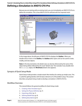
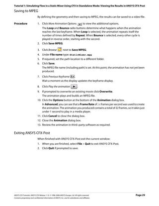
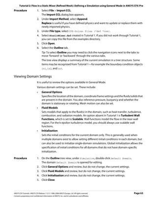
15. Creating the First Keyframe (p. 26)
16. Creating the Second Keyframe (p. 26)
17. Viewing the Animation (p. 27)
18. Modifying the Animation (p. 28)
19. Saving to MPEG (p. 29)
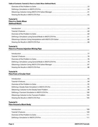
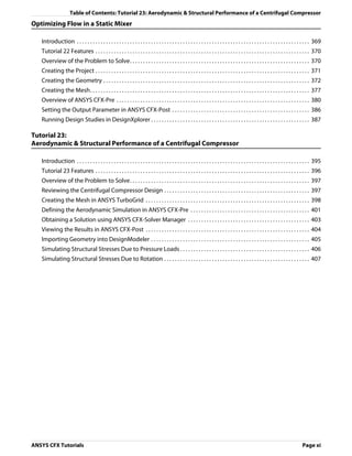
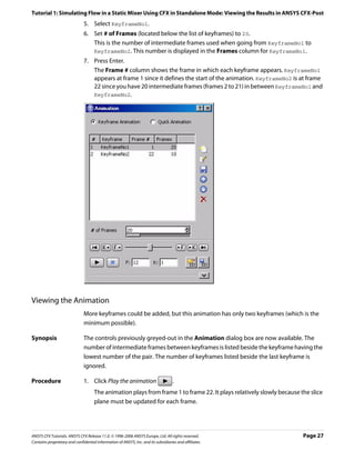
Setting the Edge Angle for a Wireframe Object
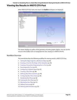
The outline of the geometry is called the wireframe or outline plot.
By default, ANSYS CFX-Post displays only some of the surface mesh. This sometimes means
that when you first load your results file, the geometry outline is not displayed clearly. You
can control the amount of the surface mesh shown by editing the Wireframe object listed
in the Outline.
The check boxes next to each object name in the Outline control the visibility of each
object. Currently only the Wireframe and Default Legend objects have visibility selected.
The edge angle determines how much of the surface mesh is visible. If the angle between
two adjacent faces is greater than the edge angle, then that edge is drawn. If the edge angle
is set to 0°, the entire surface mesh is drawn. If the edge angle is large, then only the most
significant corner edges of the geometry are drawn.
For this geometry, a setting of approximately 15° lets you view the model location without
displaying an excessive amount of the surface mesh.
In this module you can also modify the zoom settings and view of the wireframe.
Procedure 1. In the Outline, under User Locations and Plots, double-click Wireframe.
Tip: While it is not necessary to change the view to set the angle, do so to explore the
practical uses of this feature.
2. Right-click on a blank area anywhere in the viewer, select Predefined Camera from the
shortcut menu and select Isometric View (Z up).
3. In the Wireframe details view, under Definition, click in the Edge Angle box.
An embedded slider is displayed.
4. Type a value of 10 [degree].
5. Click Apply to update the object with the new setting.
Page 16 ANSYS CFX Tutorials. ANSYS CFX Release 11.0. © 1996-2006 ANSYS Europe, Ltd. All rights reserved.
Contains proprietary and confidential information of ANSYS, Inc. and its subsidiaries and affiliates.](https://image.slidesharecdn.com/ansys11tutorial-111218135319-phpapp01/85/Ansys-11-tutorial-28-320.jpg)
![Tutorial 1: Simulating Flow in a Static Mixer Using CFX in Standalone Mode: Viewing the Results in ANSYS CFX-Post
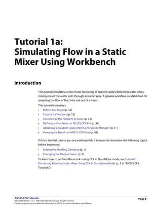
Notice that more surface mesh is displayed.
6. Drag the embedded slider to set the Edge Angle value to approximately 45 [degree].
7. Click Apply to update the object with the new setting.
Less of the outline of the geometry is displayed.
8. Type a value of 15 [degree].
9. Click Apply to update the object with the new setting.
10. Right-click on a blank area anywhere in the viewer, select Predefined Camera from the
shortcut menu and select View Towards -X.
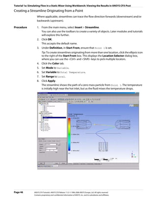
Creating a Point for the Origin of the Streamline
A streamline is the path that a particle of zero mass would follow through the domain.
Procedure 1. Select Insert > Location > Point from the main menu.
You can also use the toolbars to create a variety of objects. Later modules and tutorials
explore this further.
2. Click OK.
This accepts the default name.
3. Under Definition, ensure that Method is set to XYZ.
4. Under Point, enter the following coordinates: -1, -1, 1.
This is a point near the first inlet.
5. Click Apply.
The point appears as a symbol in the viewer as a crosshair symbol.
ANSYS CFX Tutorials. ANSYS CFX Release 11.0. © 1996-2006 ANSYS Europe, Ltd. All rights reserved. Page 17
Contains proprietary and confidential information of ANSYS, Inc. and its subsidiaries and affiliates.](https://image.slidesharecdn.com/ansys11tutorial-111218135319-phpapp01/85/Ansys-11-tutorial-29-320.jpg)


![Tutorial 1: Simulating Flow in a Static Mixer Using CFX in Standalone Mode: Viewing the Results in ANSYS CFX-Post
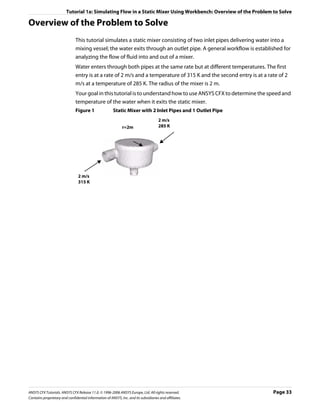
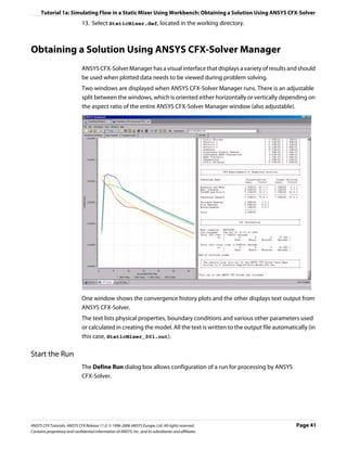
Modifying the Animation
To make the plane sweep through the whole geometry, you will set the starting position of
the plane to be at the top of the mixer. You will also modify the Range properties of the
plane so that it shows the temperature variation better. As the animation is played, you can
see the hot and cold water entering the mixer. Near the bottom of the mixer (where the
water flows out) you can see that the temperature is quite uniform. The new temperature
range lets you view the mixing process more accurately than the global range used in the
first animation.
Procedure 1. Apply the following settings to Slice
Tab Setting Value
Geometry Point 0, 0, 1.99
Color Variable Temperature
Range User Specified
Min 295 [K]
Max 305 [K]
2. Click Apply.
The slice plane moves to the top of the static mixer.
Note: Do not double click in the next step.
3. In the Animation dialog box, single click (do not double-click) KeyframeNo1 to select it.
If you had double-clicked KeyFrameNo1, the plane and viewer states would have been
redefined according to the stored settings for KeyFrameNo1. If this happens, click
Undo and try again to select the keyframe.
4. Click Set Keyframe .
The image in the Viewer replaces the one previously associated with KeyframeNo1.
5. Double-click KeyframeNo2.
The object properties for the slice plane are updated according to the settings in
KeyFrameNo2.
6. Apply the following settings to Slice
Tab Setting Value
Color Variable Temperature
Range User Specified
Min 295 [K]
Max 305 [K]
7. Click Apply.
8. In the Animation dialog box, single-click KeyframeNo2.
9. Click Set Keyframe to save the new settings to KeyframeNo2.
Page 28 ANSYS CFX Tutorials. ANSYS CFX Release 11.0. © 1996-2006 ANSYS Europe, Ltd. All rights reserved.
Contains proprietary and confidential information of ANSYS, Inc. and its subsidiaries and affiliates.](https://image.slidesharecdn.com/ansys11tutorial-111218135319-phpapp01/85/Ansys-11-tutorial-40-320.jpg)


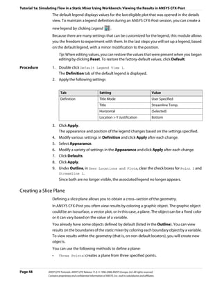
![Tutorial 1a: Simulating Flow in a Static Mixer Using Workbench: Defining a Simulation in ANSYS CFX-Pre
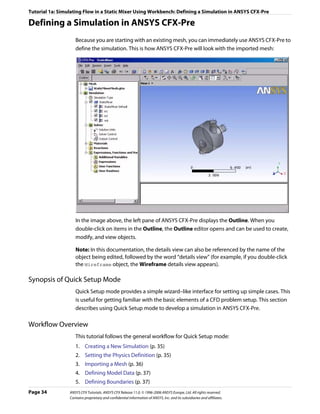
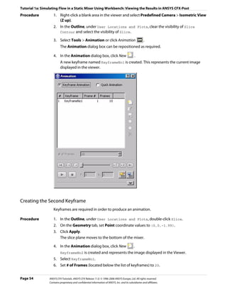
4. Right-click a blank area in the viewer and select Predefined Camera > Isometric View
(Z Up).
A clearer view of the mesh is displayed.
Defining Model Data
You need to define the type of flow and the physical models to use in the fluid domain.
You will specify the flow as steady state with turbulence and heat transfer. Turbulence is
modelled using the k - ε turbulence model and heat transfer using the thermal energy
model. The k - ε turbulence model is a commonly used model and is suitable for a wide
range of applications. The thermal energy model neglects high speed energy effects and is
therefore suitable for low speed flow applications.
Procedure 1. Ensure that Physics Definition is displayed.
2. Under Model Data, set Reference Pressure to 1 [atm].
All other pressure settings are relative to this reference pressure.
3. Set Heat Transfer to Thermal Energy.
4. Set Turbulence to k-Epsilon.
5. Click Next.
Defining Boundaries
The CFD model requires the definition of conditions on the boundaries of the domain.
Procedure 1. Ensure that Boundary Definition is displayed.
2. Delete Inlet and Outlet from the list by right-clicking each and selecting Delete.
3. Right-click in the blank area where Inlet and Outlet were listed, then select New.
4. Set Name to: in1
5. Click OK.
The boundary is created and, when selected, properties related to the boundary are
displayed.
Setting Boundary Data
Once boundaries are created, you need to create associated data. Based on Figure 1, you will
define the first inlet boundary condition to have a velocity of 2 m/s and a temperature of 315
K at one of the side inlets.
Procedure 1. Ensure that Boundary Data is displayed.
2. Set Boundary Type to Inlet.
3. Set Location to in1.
Setting Flow Specification
Once boundary data is defined, the boundary needs to have the flow specification assigned.
ANSYS CFX Tutorials. ANSYS CFX Release 11.0. © 1996-2006 ANSYS Europe, Ltd. All rights reserved. Page 37
Contains proprietary and confidential information of ANSYS, Inc. and its subsidiaries and affiliates.](https://image.slidesharecdn.com/ansys11tutorial-111218135319-phpapp01/85/Ansys-11-tutorial-49-320.jpg)
![Tutorial 1a: Simulating Flow in a Static Mixer Using Workbench: Defining a Simulation in ANSYS CFX-Pre
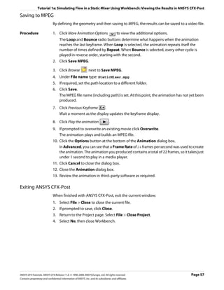
Procedure 1. Ensure that Flow Specification is displayed.
2. Set Option to Normal Speed.
3. Set Normal Speed to 2 [m s^-1].
Setting Temperature Specification
Once flow specification is defined, the boundary needs to have temperature assigned.
Procedure 1. Ensure that Temperature Specification is displayed.
2. Set Static Temperature to 315 [K].
Reviewing the Boundary Condition Definitions
Defining the boundary condition for in1 required several steps. Here the settings are
reviewed for accuracy.
Based on Figure 1, the first inlet boundary condition consists of a velocity of 2 m/s and a
temperature of 315 K at one of the side inlets.
Procedure 1. Review the boundary in1 settings for accuracy. They should be as follows:
Tab Setting Value
Boundary Data Boundary Type Inlet
Location in1
Flow Specification Option Normal Speed
Normal Speed 2 [m s^-1]
Temperature Specification Static Temperature 315 [K]
Creating the Second Inlet Boundary Definition
Based on Figure 1, you know the second inlet boundary condition consists of a velocity of 2
m/s and a temperature of 285 K at one of the side inlets. You will define that now.
Procedure 1. Under Boundary Definition, right-click in the selector area and select New.
2. Create a new boundary named in2 with these settings:
Tab Setting Value
Boundary Data Boundary Type Inlet
Location in2
Flow Specification Option Normal Speed
Normal Speed 2 [m s^-1]
Temperature Specification Static Temperature 285 [K]
Page 38 ANSYS CFX Tutorials. ANSYS CFX Release 11.0. © 1996-2006 ANSYS Europe, Ltd. All rights reserved.
Contains proprietary and confidential information of ANSYS, Inc. and its subsidiaries and affiliates.](https://image.slidesharecdn.com/ansys11tutorial-111218135319-phpapp01/85/Ansys-11-tutorial-50-320.jpg)
![Tutorial 1a: Simulating Flow in a Static Mixer Using Workbench: Defining a Simulation in ANSYS CFX-Pre
Creating the Outlet Boundary Definition
Now that the second inlet boundary has been created, the same concepts can be applied to
building the outlet boundary.
1. Create a new boundary named out with these settings:
Tab Setting Value
Boundary Data Boundary Type Outlet
Location out
Flow Specification Option Average Static Pressure
Relative Pressure 0 [Pa]
2. Click Next.
Moving to General Mode
There are no further boundary conditions that need to be set. All 2D exterior regions that
have not been assigned to a boundary condition are automatically assigned to the default
boundary condition.
Procedure 1. Set Operation to Enter General Mode and click Finish.
The three boundary conditions are displayed in the viewer as sets of arrows at the
boundary surfaces. Inlet boundary arrows are directed into the domain. Outlet
boundary arrows are directed out of the domain.
Setting Solver Control
Solver Control parameters control aspects of the numerical solution generation process.
While an upwind advection scheme is less accurate than other advection schemes, it is also
more robust. This advection scheme is suitable for obtaining an initial set of results, but in
general should not be used to obtain final accurate results.
The time scale can be calculated automatically by the solver or set manually. The Automatic
option tends to be conservative, leading to reliable, but often slow, convergence. It is often
possible to accelerate convergence by applying a time scale factor or by choosing a manual
value that is more aggressive than the Automatic option. In this tutorial, you will select a
physical time scale, leading to convergence that is twice as fast as the Automatic option.
Procedure 1. Click Solver Control .
2. On the Basic Settings tab, set Advection Scheme > Option to Upwind.
3. Set Convergence Control > Fluid Timescale Control > Timescale Control to
Physical Timescale and set the physical timescale value to 2 [s].
4. Click OK.
ANSYS CFX Tutorials. ANSYS CFX Release 11.0. © 1996-2006 ANSYS Europe, Ltd. All rights reserved. Page 39
Contains proprietary and confidential information of ANSYS, Inc. and its subsidiaries and affiliates.](https://image.slidesharecdn.com/ansys11tutorial-111218135319-phpapp01/85/Ansys-11-tutorial-51-320.jpg)
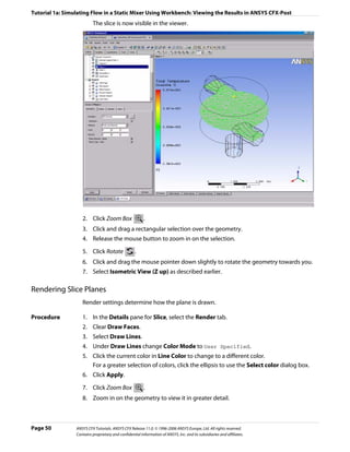
![Tutorial 1a: Simulating Flow in a Static Mixer Using Workbench: Viewing the Results in ANSYS CFX-Post
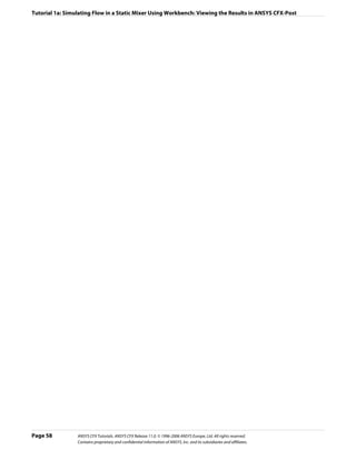
Setting the Edge Angle for a Wireframe Object
The outline of the geometry is called the wireframe or outline plot.
By default, ANSYS CFX-Post displays only some of the surface mesh. This sometimes means
that when you first load your results file, the geometry outline is not displayed clearly. You
can control the amount of the surface mesh shown by editing the Wireframe object listed
in the Outline.
The check boxes next to each object name in the Outline control the visibility of each
object. Currently only the Wireframe and Default Legend objects have visibility selected.
The edge angle determines how much of the surface mesh is visible. If the angle between
two adjacent faces is greater than the edge angle, then that edge is drawn. If the edge angle
is set to 0°, the entire surface mesh is drawn. If the edge angle is large, then only the most
significant corner edges of the geometry are drawn.
For this geometry, a setting of approximately 15° lets you view the model location without
displaying an excessive amount of the surface mesh.
In this module you can also modify the zoom settings and view of the wireframe.
Procedure 1. In the Outline, under User Locations and Plots, double-click Wireframe.
Tip: While it is not necessary to change the view to set the angle, do so to explore the
practical uses of this feature.
2. Right-click on a blank area anywhere in the viewer, select Predefined Camera from the
shortcut menu and select Isometric View (Z up).
3. In the Wireframe details view, under Definition, click in the Edge Angle box.
An embedded slider is displayed.
4. Type a value of 10 [degree].
5. Click Apply to update the object with the new setting.
Page 44 ANSYS CFX Tutorials. ANSYS CFX Release 11.0. © 1996-2006 ANSYS Europe, Ltd. All rights reserved.
Contains proprietary and confidential information of ANSYS, Inc. and its subsidiaries and affiliates.](https://image.slidesharecdn.com/ansys11tutorial-111218135319-phpapp01/85/Ansys-11-tutorial-56-320.jpg)
![Tutorial 1a: Simulating Flow in a Static Mixer Using Workbench: Viewing the Results in ANSYS CFX-Post
Notice that more surface mesh is displayed.
6. Drag the embedded slider to set the Edge Angle value to approximately 45 [degree].
7. Click Apply to update the object with the new setting.
Less of the outline of the geometry is displayed.
8. Type a value of 15 [degree].
9. Click Apply to update the object with the new setting.
10. Right-click on a blank area anywhere in the viewer, select Predefined Camera from the
shortcut menu and select View Towards -X.
Creating a Point for the Origin of the Streamline
A streamline is the path that a particle of zero mass would follow through the domain.
Procedure 1. Select Insert > Location > Point from the main menu.
You can also use the toolbars to create a variety of objects. Later modules and tutorials
explore this further.
2. Click OK.
This accepts the default name.
3. Under Definition, ensure that Method is set to XYZ.
4. Under Point, enter the following coordinates: -1, -1, 1.
This is a point near the first inlet.
5. Click Apply.
The point appears as a symbol in the viewer as a crosshair symbol.
ANSYS CFX Tutorials. ANSYS CFX Release 11.0. © 1996-2006 ANSYS Europe, Ltd. All rights reserved. Page 45
Contains proprietary and confidential information of ANSYS, Inc. and its subsidiaries and affiliates.](https://image.slidesharecdn.com/ansys11tutorial-111218135319-phpapp01/85/Ansys-11-tutorial-57-320.jpg)


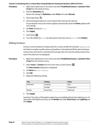

![Tutorial 1a: Simulating Flow in a Static Mixer Using Workbench: Viewing the Results in ANSYS CFX-Post
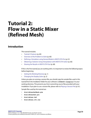
Modifying the Animation
To make the plane sweep through the whole geometry, you will set the starting position of
the plane to be at the top of the mixer. You will also modify the Range properties of the
plane so that it shows the temperature variation better. As the animation is played, you can
see the hot and cold water entering the mixer. Near the bottom of the mixer (where the
water flows out) you can see that the temperature is quite uniform. The new temperature
range lets you view the mixing process more accurately than the global range used in the
first animation.
Procedure 1. Apply the following settings to Slice
Tab Setting Value
Geometry Point 0, 0, 1.99
Color Mode Variable
Range User Specified
Min 295 [K]
Max 305 [K]
2. Click Apply.
The slice plane moves to the top of the static mixer.
Note: Do not double click in the next step.
3. In the Animation dialog box, single click (do not double-click) KeyframeNo1 to select it.
If you had double-clicked KeyFrameNo1, the plane and viewer states would have been
redefined according to the stored settings for KeyFrameNo1. If this happens, click
Undo and try again to select the keyframe.
4. Click Set Keyframe .
The image in the Viewer replaces the one previously associated with KeyframeNo1.
5. Double-click KeyframeNo2.
The object properties for the slice plane are updated according to the settings in
KeyFrameNo2.
6. Apply the following settings to Slice
Tab Setting Value
Color Mode Variable
Range User Specified
Min 295 [K]
Max 305 [K]
7. Click Apply.
8. In the Animation dialog box, single-click KeyframeNo2.
9. Click Set Keyframe to save the new settings to KeyframeNo2.
Page 56 ANSYS CFX Tutorials. ANSYS CFX Release 11.0. © 1996-2006 ANSYS Europe, Ltd. All rights reserved.
Contains proprietary and confidential information of ANSYS, Inc. and its subsidiaries and affiliates.](https://image.slidesharecdn.com/ansys11tutorial-111218135319-phpapp01/85/Ansys-11-tutorial-68-320.jpg)
![Tutorial 2: Flow in a Static Mixer (Refined Mesh): Defining a Simulation using General Mode in ANSYS CFX-Pre
Viewing the Boundary Condition Setting
For the k-epsilon turbulence model, you must specify the turbulent nature of the flow
entering through the inlet boundary. For this simulation, the default setting of Medium
(Intensity = 5%) is used. This is a sensible setting if you do not know the turbulence
properties of the incoming flow.
Procedure 1. Under Default Domain, double-click in1.
2. Click the Boundary Details tab and review the settings for Flow Regime, Mass and
Momentum, Turbulence and Heat Transfer.
3. Click Close.
Defining Solver Parameters
Solver Control parameters control aspects of the numerical-solution generation process.
In Tutorial 1 you set some solver control parameters, such as Advection Scheme and
Timescale Control, while other parameters were set automatically by ANSYS CFX-Pre.
In this tutorial, High Resolution is used for the advection scheme. This is more accurate
than the Upwind Scheme used in Tutorial 1. You usually require a smaller timestep when
using this model. You can also expect the solution to take a higher number of iterations to
converge when using this model.
Procedure 1. Select Insert > Solver > Solver Control from the main menu or click Solver Control .
2. Apply the following Basic Settings
Setting Value
Advection Scheme > Option High Resolution
Convergence Control > Max. Iterations* 150
Convergence Control > Fluid Timescale Control > Physical Timescale
Timescale Control
Convergence Control > Fluid Timescale Control > Physical 0.5 [s]
Timescale
*. If your solution does not meet the convergence criteria after this number of
timesteps, the ANSYS CFX-Solver will stop.
3. Click Apply.
4. Click the Advanced Options tab.
5. Ensure that Global Dynamic Model Control is selected.
6. Click OK.
Writing the Solver (.def) File
Once all boundaries are created you move from ANSYS CFX-Pre into ANSYS CFX-Solver.
Page 64 ANSYS CFX Tutorials. ANSYS CFX Release 11.0. © 1996-2006 ANSYS Europe, Ltd. All rights reserved.
Contains proprietary and confidential information of ANSYS, Inc. and its subsidiaries and affiliates.](https://image.slidesharecdn.com/ansys11tutorial-111218135319-phpapp01/85/Ansys-11-tutorial-76-320.jpg)

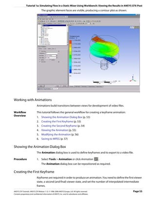
![Tutorial 2: Flow in a Static Mixer (Refined Mesh): Viewing the Results in ANSYS CFX-Post
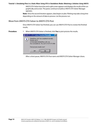
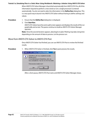
After a short pause, ANSYS CFX-Post starts.
Viewing the Results in ANSYS CFX-Post
In the following sections, you will explore the differences between the mesh and the results
from this tutorial and tutorial 1.
Creating a Slice Plane
More information exists for use by ANSYS CFX-Post in this tutorial than in Tutorial 1 because
the slice plane is more detailed.
Once a new slice plane is created it can be compared with Tutorial 1. There are three
noticeable differences between the two slice planes.
• Around the edges of the mixer geometry there are several layers of narrow rectangles.
This is the region where the mesh contains prismatic elements (which are created as
inflation layers). The bulk of the geometry contains tetrahedral elements.
• There are more lines on the plane than there were in Tutorial 1. This is because the slice
plane intersects with more mesh elements.
• The curves of the mixer are smoother than in Tutorial 1 because the finer mesh better
represents the true geometry.
Procedure 1. Right-click a blank area in the viewer and select Predefined Camera > Isometric View
(Z up).
2. From the main menu, select Insert > Location > Plane or under Location, click Plane.
3. In the Insert Plane dialog box, type Slice and click OK.
The Geometry, Color, Render and View tabs let you switch between settings.
4. Apply the following settings
Tab Setting Value
Geometry Domains Default Domain
Definition > Method XY Plane
Definition > Z 1 [m]
Render Draw Faces (Cleared)
Draw Lines (Selected)
5. Click Apply.
6. Right-click a blank area in the viewer and select Predefined Camera > View Towards
-Z.
7. Click Zoom Box .
8. Zoom in on the geometry to view it in greater detail.
Page 68 ANSYS CFX Tutorials. ANSYS CFX Release 11.0. © 1996-2006 ANSYS Europe, Ltd. All rights reserved.
Contains proprietary and confidential information of ANSYS, Inc. and its subsidiaries and affiliates.](https://image.slidesharecdn.com/ansys11tutorial-111218135319-phpapp01/85/Ansys-11-tutorial-80-320.jpg)
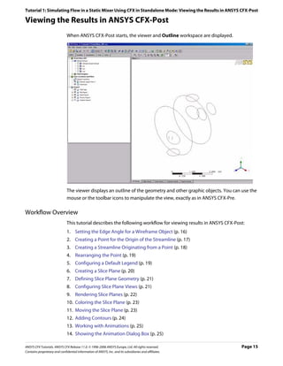
![Tutorial 2: Flow in a Static Mixer (Refined Mesh): Viewing the Results in ANSYS CFX-Post
3. On the right side of the dialog box, there are two frames. Under Results file option,
select Add to current results.
4. Select the Offset in Y direction check box.
5. Under Additional actions, ensure that the Clear user state before loading check box
is cleared.
6. Click Open to load the results.
In the tree view, there is now a second group of domains, meshes and boundary
conditions with the heading StaticMixer_001.
7. Double-click the Wireframe object under User Locations and Plots.
8. In the Definition tab, set Edge Angle to 5 [degree].
9. Click Apply.
10. Right-click a blank area in the viewer and select Predefined Camera > Isometric View
(Z up).
Both meshes are now displayed in a line along the Y axis. Notice that one mesh is of a
higher resolution than the other.
11. Set Edge Angle to 30 [degree].
12. Click Apply.
Creating a Second Slice Plane
Procedure 1. In the tree view, right-click the plane named Slice and select Duplicate.
2. Click OK to accept the default name Slice 1.
3. In the tree view, double-click the plane named Slice 1.
4. On the Geometry tab, set Domains to Default Domain 1.
5. On the Color tab, ensure that Range is set to Global.
6. Click Apply.
7. Double-click Slice and make sure that Range is set to Global.
Comparing Slice Planes using Multiple Views
Procedure 1. Select the option with the two vertical rectangles. Notice that the Viewer now has two
separate views.
The visibility status of each object is maintained separately for each view or figure that
can be displayed in a given viewport. This allows some planes to be shown while others
are hidden.
Page 70 ANSYS CFX Tutorials. ANSYS CFX Release 11.0. © 1996-2006 ANSYS Europe, Ltd. All rights reserved.
Contains proprietary and confidential information of ANSYS, Inc. and its subsidiaries and affiliates.](https://image.slidesharecdn.com/ansys11tutorial-111218135319-phpapp01/85/Ansys-11-tutorial-82-320.jpg)
![Tutorial 2: Flow in a Static Mixer (Refined Mesh): Viewing the Results in ANSYS CFX-Post
5. Click Zoom Box .
6. Zoom in on the geometry to view out in greater detail.
7. Click Rotate on the Viewing Tools toolbar.
8. Rotate the image as required to clearly see the mesh.
Looking at the Inflated Elements in Three Dimensions
To show more clearly what effect inflation has on the shape of the elements, you will use
volume objects to show two individual elements. The first element that will be shown is a
normal tetrahedral element; the second is a prismatic element from an inflation layer of the
mesh.
Leave the surface mesh on the outlet visible to help see how surface and volume meshes are
related.
Procedure 1. From the main menu, select Insert > Location > Volume or, under Location click
Volume.
2. In the Insert Volume dialog box, type Tet Volume and click OK.
3. Apply the following settings
Tab Setting Value
Geometry Definition > Method Sphere
Definition > Point * 0.08, 0, -2
Definition > Radius 0.14 [m]
Definition > Mode Below Intersection
Inclusive† (Cleared)
Color Color Red
Render Draw Faces > Transparency 0.3
Draw Lines (Selected)
Draw Lines > Line Width 1
Draw Lines > Color Mode User Specified
Draw Lines > Line Color Grey
*. The z slider’s minimum value corresponds to the minimum z value of the entire
geometry, which, in this case, occurs at the outlet.
†. Only elements that are entirely contained within the sphere volume will be
included.
4. Click Apply to create the volume object.
5. Right-click Tet Volume and choose Duplicate.
6. In the Duplicate Tet Volume dialog box, type Prism Volume and click OK.
7. Double-click Prism Volume.
8. Apply the following settings
Page 72 ANSYS CFX Tutorials. ANSYS CFX Release 11.0. © 1996-2006 ANSYS Europe, Ltd. All rights reserved.
Contains proprietary and confidential information of ANSYS, Inc. and its subsidiaries and affiliates.](https://image.slidesharecdn.com/ansys11tutorial-111218135319-phpapp01/85/Ansys-11-tutorial-84-320.jpg)
![Tutorial 2: Flow in a Static Mixer (Refined Mesh): Viewing the Results in ANSYS CFX-Post
Tab Setting Value
Geometry Definition > Point -0.22, 0.4, -1.85
Definition > Radius 0.206 [m]
Color Color Orange
9. Click Apply.
Viewing the Surface Mesh on the Mixer Body
Procedure 1. Double-click the Default Domain Default object.
2. Apply the following settings
Tab Setting Value
Render Draw Faces (Selected)
Draw Lines (Selected)
Line Width 2
3. Click Apply.
Viewing the Layers of Inflated Elements on a Plane
You will see the layers of inflated elements on the wall of the main body of the mixer. Within
the body of the mixer, there will be many lines that are drawn wherever the face of a mesh
element intersects the slice plane.
Procedure 1. From the main menu, select Insert > Location > Plane or under Location, click Plane.
2. In the Insert Plane dialog box, type Slice 2 and click OK.
3. Apply the following settings
Tab Setting Value
Geometry Definition > Method YZ Plane
Definition > X 0 [m]
Render Draw Faces (Cleared)
Draw Lines (Selected)
4. Click Apply.
5. Turn off the visibility of all objects except Slice 2.
6. To see the plane clearly, right-click in the viewer and select Predefined Camera > View
Towards -X.
Viewing the Mesh Statistics
You can use the Report Viewer to check the quality of your mesh. For example, you can load
a .def file into ANSYS CFX-Post and check the mesh quality before running the .def file in
the solver.
ANSYS CFX Tutorials. ANSYS CFX Release 11.0. © 1996-2006 ANSYS Europe, Ltd. All rights reserved. Page 73
Contains proprietary and confidential information of ANSYS, Inc. and its subsidiaries and affiliates.](https://image.slidesharecdn.com/ansys11tutorial-111218135319-phpapp01/85/Ansys-11-tutorial-85-320.jpg)
![Tutorial 2: Flow in a Static Mixer (Refined Mesh): Viewing the Results in ANSYS CFX-Post
Procedure 1. Click the Report Viewer tab (located below the viewer window).
A report appears. Look at the table shown in the “Mesh Report” section.
2. Double-click Report > Mesh Report in the Outline tree view.
3. In the Mesh Report details view, select Statistics > Maximum Face Angle.
4. Click Refresh Preview.
Note that a new table, showing the maximum face angle for all elements in the mesh,
has been added to the “Mesh Report” section of the report. The maximum face angle is
reported as 148.95°.
As a result of generating this mesh statistic for the report, a new variable, Maximum Face
Angle, has been created and stored at every node. This variable will be used in the next
section.
Viewing the Mesh Elements with Largest Face Angle
In this section, you will visualize the mesh elements that have a Maximum Face Angle value
greater than 140°.
Procedure 1. Click the 3D Viewer tab (located below the viewer window).
2. Right-click a blank area in the viewer and select Predefined Camera > Isometric View
(Z up).
3. In the Outline tree view, select the visibility check box of Wireframe.
4. From the main menu, select Insert > Location > Volume or under Location, click
Volume.
5. In the Insert Volume dialog box, type Max Face Angle Volume and click OK.
6. Apply the following settings
Tab Setting Value
Geometry Definition > Method Isovolume
Definition > Variable Maximum Face Angle*
Definition > Mode Above Value
Definition > Value 140 [degree]
Inclusive† (Selected)
*. Select Maximum Face Angle from the larger list of variables available by clicking
to the right of the Variable box.
†. This includes any elements that have at least one node with a variable value greater
than or equal to the given value.
7. Click Apply.
The volume object appears in the viewer.
Page 74 ANSYS CFX Tutorials. ANSYS CFX Release 11.0. © 1996-2006 ANSYS Europe, Ltd. All rights reserved.
Contains proprietary and confidential information of ANSYS, Inc. and its subsidiaries and affiliates.](https://image.slidesharecdn.com/ansys11tutorial-111218135319-phpapp01/85/Ansys-11-tutorial-86-320.jpg)

![Tutorial 3: Flow in a Process Injection Mixing Pipe: Defining a Simulation using General Mode in ANSYS CFX-Pre
Procedure 1. Select File > Import Mesh.
2. From your tutorial directory, select InjectMixerMesh.gtm.
3. Click Open.
4. Right-click a blank area in the viewer and select Predefined Camera > Isometric View
(Y up) from the shortcut menu.
Setting Temperature-Dependent Material Properties
You will create an expression for viscosity as a function of temperature and then use this
expression to modify the properties of the library material: Water.
Viscosity will be made to vary linearly with temperature between the following conditions:
• µ =1.8E-03 N s m-2 at T=275.0 K
• µ =5.45E-04 N s m-2 at T=325.0 K
The variable T (Temperature) is a ANSYS CFX System Variable recognized by ANSYS CFX-Pre,
denoting static temperature. All variables, expressions, locators, functions, and constants
can be viewed by double-clicking the appropriate entry (such as Additional Variables
or Expressions) in the tree view.
All expressions must have consistent units. You should be careful if using temperature in an
expression with units other than [K].
The Expressions tab lets you define, modify, evaluate, plot, copy, delete and browse
through expressions used within ANSYS CFX-Pre.
Procedure 1. From the main menu, select Insert > Expressions, Functions and Variables >
Expression.
2. In the New Expression dialog box, type Tupper.
3. Click OK.
The details view for the Tupper equation is displayed.
4. Under Definition, type 325 [K].
5. Click Apply to create the expression.
The expression is added to the list of existing expressions.
6. Right-click in the Expressions workspace and select New.
7. In the New Expression dialog box, type Tlower.
8. Click OK.
9. Under Definition, type 275 [K].
10. Click Apply to create the expression.
The expression is added to the list of existing expressions.
11. Create expressions for Visupper, Vislower and VisT using the following values.
Name Definition
Visupper 5.45E-04 [N s m^-2]
Vislower 1.8E-03 [N s m^-2]
VisT Vislower+(Visupper-Vislower)*(T-Tlower)/(Tupper-Tlower)
ANSYS CFX Tutorials. ANSYS CFX Release 11.0. © 1996-2006 ANSYS Europe, Ltd. All rights reserved. Page 81
Contains proprietary and confidential information of ANSYS, Inc. and its subsidiaries and affiliates.](https://image.slidesharecdn.com/ansys11tutorial-111218135319-phpapp01/85/Ansys-11-tutorial-93-320.jpg)
![Tutorial 3: Flow in a Process Injection Mixing Pipe: Defining a Simulation using General Mode in ANSYS CFX-Pre
Plotting an Expression
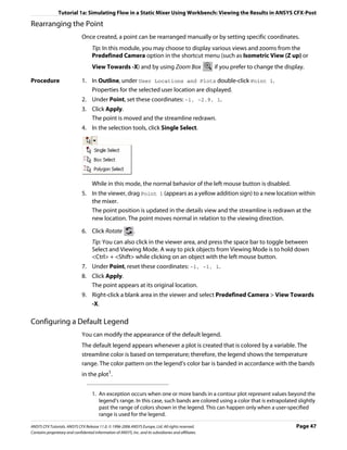
Procedure 1. Right-click VisT in the Expressions tree view, and then select Edit.
The Expressions details view for VisT appears.
Tip: Alternatively, double-clicking the expression also opens the Expressions details
view.
2. Click the Plot tab and apply the following settings
Tab Setting Value
Plot Number of Points 10
T (Selected)
Start of Range 275 [K]
End of Range 325 [K]
3. Click Plot Expression.
A plot showing the variation of the expression VisT with the variable T is displayed.
Evaluating an Expression
Procedure 1. Click the Evaluate tab.
2. In T, type 300 [K].
This is between the start and end range defined in the last module.
3. Click Evaluate Expression.
The value of VisT for the given value of T appears in the Value field.
Modify Material Properties
Default material properties (such as those of Water) can be modified when required.
Procedure 1. Click the Outline tab.
2. Double click Water under Materials to display the Basic Settings tab.
3. Click the Material Properties tab.
4. Expand Transport Properties.
5. Select Dynamic Viscosity.
6. Under Dynamic Viscosity, click in Dynamic Viscosity.
7. Click Enter Expression .
8. Enter the expression VisT into the data box.
9. Click OK.
Creating the Domain
The domain will be set to use the thermal energy heat transfer model, and the k-ε
(k-epsilon) turbulence model.
Page 82 ANSYS CFX Tutorials. ANSYS CFX Release 11.0. © 1996-2006 ANSYS Europe, Ltd. All rights reserved.
Contains proprietary and confidential information of ANSYS, Inc. and its subsidiaries and affiliates.](https://image.slidesharecdn.com/ansys11tutorial-111218135319-phpapp01/85/Ansys-11-tutorial-94-320.jpg)
![Tutorial 3: Flow in a Process Injection Mixing Pipe: Defining a Simulation using General Mode in ANSYS CFX-Pre
Both General Options and Fluid Models are changed in this module. The Initialization tab
is for setting domain-specific initial conditions, which are not used in this tutorial. Instead,
global initialization is used to set the starting conditions.
Procedure 1. Select Insert > Domain from the main menu or click Domain .
2. In the Insert Domain dialog box, type InjectMixer.
3. Click OK.
4. Apply the following settings
Tab Setting Value
General Options Basic Settings > Location B1.P3
Basic Settings > Fluids List Water
Domain Models > Pressure > 0 [atm]
Reference Pressure
5. Click Fluid Models.
6. Apply the following settings
Setting Value
Heat Transfer > Option Thermal Energy
7. Click OK.
Creating the Side Inlet Boundary Conditions
The side inlet boundary condition needs to be defined.
Procedure 1. Select Insert > Boundary Condition from the main menu or click Boundary Condition
.
2. Set Name to side inlet.
3. Click OK.
4. Apply the following settings
Tab Setting Value
Basic Settings Boundary Type Inlet
Location side inlet
Boundary Details Mass and Momentum > Option Normal Speed
Normal Speed 5 [m s^-1]
Heat Transfer > Option Static Temperature
Static Temperature 315 [K]
5. Click OK.
ANSYS CFX Tutorials. ANSYS CFX Release 11.0. © 1996-2006 ANSYS Europe, Ltd. All rights reserved. Page 83
Contains proprietary and confidential information of ANSYS, Inc. and its subsidiaries and affiliates.](https://image.slidesharecdn.com/ansys11tutorial-111218135319-phpapp01/85/Ansys-11-tutorial-95-320.jpg)
![Tutorial 3: Flow in a Process Injection Mixing Pipe: Defining a Simulation using General Mode in ANSYS CFX-Pre
Creating the Main Inlet Boundary Conditions
The main inlet boundary condition needs to be defined. This inlet is defined using a velocity
profile found in the example directory. Profile data needs to be initialized before the
boundary condition can be created.
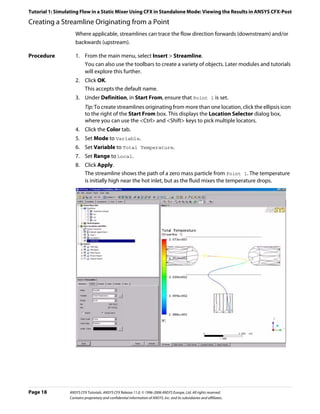
You will create a plot showing the velocity profile data, marked by higher velocities near the
center of the inlet, and lower velocities near the inlet walls.
Procedure 1. Select Tools > Initialize Profile Data.
2. Under Data File, click Browse .
3. From your working directory, select InjectMixer_velocity_profile.csv.
4. Click Open.
5. Click OK.
The profile data is read into memory.
6. Select Insert > Boundary Condition from the main menu or click Boundary Condition
.
7. Set name Name to main inlet.
8. Click OK.
9. Apply the following settings
Tab Setting Value
Basic Settings Boundary Type Inlet
Location main inlet
Profile Boundary Conditions (Selected)
> Use Profile Data
Profile Boundary Setup > main inlet
Profile Name
10. Click Generate Values.
This causes the profile values of U, V, W to be applied at the nodes on the main inlet
boundary, and U, V, W entries to be made in Boundary Details. To later modify the
velocity values at the main inlet and reset values to those read from the BC Profile file,
revisit Basic Settings for this boundary condition and click Generate Values.
11. Apply the following settings
Tab Setting Value
Boundary Details Flow Regime > Option Subsonic
Turbulence > Option Medium (Intensity = 5%)
Heat Transfer > Option Static Temperature
Static Temperature 285 [K]
Plot Options Boundary Contour (Selected)
Profile Variable W
12. Click OK.
Page 84 ANSYS CFX Tutorials. ANSYS CFX Release 11.0. © 1996-2006 ANSYS Europe, Ltd. All rights reserved.
Contains proprietary and confidential information of ANSYS, Inc. and its subsidiaries and affiliates.](https://image.slidesharecdn.com/ansys11tutorial-111218135319-phpapp01/85/Ansys-11-tutorial-96-320.jpg)
![Tutorial 3: Flow in a Process Injection Mixing Pipe: Defining a Simulation using General Mode in ANSYS CFX-Pre
13. Zoom into the main inlet to view the inlet velocity contour.
Creating the Main Outlet Boundary Condition
In this module you create the outlet boundary condition. All other surfaces which have not
been explicitly assigned a boundary condition will remain in the InjectMixer Default
object, which is shown in the tree view. This boundary condition uses a No-Slip
Adiabatic Wall by default.
Procedure 1. Select Insert > Boundary Condition from the main menu or click Boundary Condition
.
2. Set Name to outlet.
3. Click OK.
4. Apply the following settings
Tab Setting Value
Basic Settings Boundary Type Outlet
Location outlet
Boundary Details Flow Regime > Option Subsonic
Mass and Momentum > Option Average Static Pressure
Relative Pressure 0 [Pa]
5. Click OK.
Setting Initial Values
Procedure 1. Click Global Initialization .
2. Select Turbulence Eddy Dissipation.
3. Click OK.
Setting Solver Control
Procedure 1. Click Solver Control .
2. Apply the following settings
ANSYS CFX Tutorials. ANSYS CFX Release 11.0. © 1996-2006 ANSYS Europe, Ltd. All rights reserved. Page 85
Contains proprietary and confidential information of ANSYS, Inc. and its subsidiaries and affiliates.](https://image.slidesharecdn.com/ansys11tutorial-111218135319-phpapp01/85/Ansys-11-tutorial-97-320.jpg)
![Tutorial 3: Flow in a Process Injection Mixing Pipe: Defining a Simulation using General Mode in ANSYS CFX-Pre
Tab Setting Value
Basic Settings Advection Scheme > Option Specified Blend Factor
Advection Scheme > Blend 0.75
Factor
Convergence Control > Max. 50
Iterations
Convergence Control > Physical Timescale
Fluid Timescale Control >
Timescale Control
Convergence Control > 2 [s]
Fluid Timescale Control >
Physical Timescale
Convergence Criteria > RMS
Residual Type
Convergence Criteria > 1.E-4*
Residual Target
*. An RMS value of at least 1.E-5 is usually required for adequate convergence, but the
default value is sufficient for demonstration purposes.
3. Click OK.
Writing the Solver (.def) File
Once the problem has been defined you move from General Mode into ANSYS CFX-Solver.
Procedure 1. Click Write Solver File .
The Write Solver File dialog box appears.
2. Apply the following settings:
Setting Value
File name InjectMixer.def
Quit CFX–Pre* (Selected)
*. If using ANSYS CFX-Pre in Standalone Mode.
3. Ensure Start Solver Manager is selected and click Save.
4. If you are notified the file already exists, click Overwrite.
This file is provided in the tutorial directory and may exist in your working folder if you
have copied it there.
5. If prompted, click Yes or Save & Quit to save InjectMixer.cfx.
The definition file (InjectMixer.def), mesh file (InjectMixer.gtm) and the
simulation file (InjectMixer.cfx) are created. ANSYS CFX-Solver Manager
automatically starts and the definition file is set in the Definition File box of Define
Run.
6. Proceed to Obtaining a Solution Using ANSYS CFX-Solver Manager (p. 87).
Page 86 ANSYS CFX Tutorials. ANSYS CFX Release 11.0. © 1996-2006 ANSYS Europe, Ltd. All rights reserved.
Contains proprietary and confidential information of ANSYS, Inc. and its subsidiaries and affiliates.](https://image.slidesharecdn.com/ansys11tutorial-111218135319-phpapp01/85/Ansys-11-tutorial-98-320.jpg)
![Tutorial 3: Flow in a Process Injection Mixing Pipe: Viewing the Results in ANSYS CFX-Post
Moving from ANSYS CFX-Solver Manager to ANSYS CFX-Post
1. Select Tools > Post–Process Results or click Post–Process Results .
2. If using ANSYS CFX-Solver Manager in standalone mode, optionally select Shut down
Solver Manager.
3. Click OK.
Viewing the Results in ANSYS CFX-Post
When ANSYS CFX-Post starts, the viewer and Outline workspace display by default.
Workflow Overview
This section provides a brief summary of the topics to follow as a general workflow:
1. Modifying the Outline of the Geometry (p. 88)
2. Creating and Modifying Streamlines (p. 88)
3. Modifying Streamline Color Ranges (p. 89)
4. Coloring Streamlines with a Constant Color (p. 89)
5. Duplicating and Modifying a Streamline Object (p. 90)
6. Examining Turbulent Kinetic Energy (p. 90)
Modifying the Outline of the Geometry
Throughout this and the following examples, use your mouse and the Viewing Tools
toolbar to manipulate the geometry as required at any time.
Procedure 1. In the tree view, double click Wireframe.
2. Set the Edge Angle to 15 [degree].
3. Click Apply.
Creating and Modifying Streamlines
When you complete this module you will see streamlines (mainly blue and green) starting
at the main inlet of the geometry and proceeding to the outlet. Above where the side pipe
meets the main pipe, there is an area where the flow re-circulates rather than flowing
roughly tangent to the direction of the pipe walls.
Procedure 1. Select Insert > Streamline from the main menu or click Streamline .
2. Under Name, type MainStream.
3. Click OK.
4. Apply the following settings
Page 88 ANSYS CFX Tutorials. ANSYS CFX Release 11.0. © 1996-2006 ANSYS Europe, Ltd. All rights reserved.
Contains proprietary and confidential information of ANSYS, Inc. and its subsidiaries and affiliates.](https://image.slidesharecdn.com/ansys11tutorial-111218135319-phpapp01/85/Ansys-11-tutorial-100-320.jpg)
![Tutorial 3: Flow in a Process Injection Mixing Pipe: Viewing the Results in ANSYS CFX-Post
Tab Setting Value
Geometry Type 3D Streamline
Definition > Start From main inlet
5. Click Apply.
6. Right-click a blank area in the viewer, select Predefined Camera from the shortcut
menu, then select Isometric View (Y up).
The pipe is displayed with the main inlet in the bottom right of the viewer.
Modifying Streamline Color Ranges
You can change the appearance of the streamlines using the Range setting on the Color
tab.
Procedure 1. Under User Locations and Plots, modify the streamline object MainStream by
applying the following settings
Tab Setting Value
Color Range Local
2. Click Apply.
The color map is fitted to the range of velocities found along the streamlines. The
streamlines therefore collectively contain every color in the color map.
3. Apply the following settings
Tab Setting Value
Color Range User Specified
Min 0.2 [m s^-1]
Max 2.2 [m s^-1]
Note: Portions of streamlines that have values outside the range shown in the legend are
colored according to the color at the nearest end of the legend. When using tubes or
symbols (which contain faces), more accurate colors are obtained with lighting turned off.
4. Click Apply.
The streamlines are colored using the specified range of velocity values.
Coloring Streamlines with a Constant Color
1. Apply the following settings
Tab Setting Value
Color Mode Constant
Color (Green)
ANSYS CFX Tutorials. ANSYS CFX Release 11.0. © 1996-2006 ANSYS Europe, Ltd. All rights reserved. Page 89
Contains proprietary and confidential information of ANSYS, Inc. and its subsidiaries and affiliates.](https://image.slidesharecdn.com/ansys11tutorial-111218135319-phpapp01/85/Ansys-11-tutorial-101-320.jpg)
![Tutorial 3: Flow in a Process Injection Mixing Pipe: Viewing the Results in ANSYS CFX-Post
Color can be set to green by selecting it from the color pallet, or by repeatedly clicking
on the color box until it cycles through to the default green color.
2. Click Apply.
Duplicating and Modifying a Streamline Object
Any object can be duplicated to create a copy for modification without altering the original.
Procedure 1. Right-click MainStream and select Duplicate from the shortcut menu.
2. In the Name window, type SideStream.
3. Click OK.
4. Double click on the newly created streamline, SideStream.
5. Apply the following settings
Tab Setting Value
Geometry Definition > Start From side inlet
Color Mode Constant
Color (Red)
6. Click Apply.
Red streamlines appear, starting from the side inlet.
7. For better view, select Isometric View (Y up).
Examining Turbulent Kinetic Energy
A common way of viewing various quantities within the domain is to use a slice plane, as
demonstrated in this module.
Note: This module has multiple changes compiled into single steps in preparation for other
tutorials that provide fewer specific instructions.
Procedure 1. Clear visibility for both the MainStream and the SideStream objects.
2. Create a plane named Plane 1 that is normal to X and passing through the X = 0 Point.
To do so, specific instructions follow.
a. From the main menu, select Insert > Location > Plane and click OK.
b. In the Details view set Definition > Method to YZ Plane and X to 0 [m].
c. Click Apply.
3. Color the plane using the variable Turbulence Kinetic Energy, to show regions of
high turbulence. To do so, apply the settings below.
Tab Setting Value
Color Mode Variable
Variable Turbulence Kinetic Energy
4. Click Apply.
Page 90 ANSYS CFX Tutorials. ANSYS CFX Release 11.0. © 1996-2006 ANSYS Europe, Ltd. All rights reserved.
Contains proprietary and confidential information of ANSYS, Inc. and its subsidiaries and affiliates.](https://image.slidesharecdn.com/ansys11tutorial-111218135319-phpapp01/85/Ansys-11-tutorial-102-320.jpg)


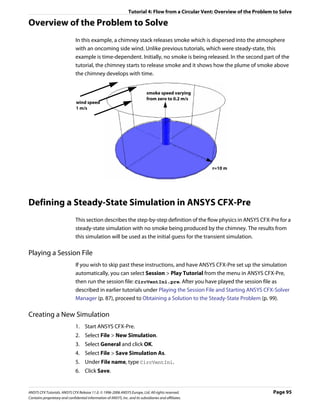
![Tutorial 4: Flow from a Circular Vent: Defining a Steady-State Simulation in ANSYS CFX-Pre
Importing the Mesh
1. Select File > Import Mesh.
2. From your working directory, select CircVentMesh.gtm.
3. Click Open.
4. Right-click a blank area in the viewer and select Predefined Camera > Isometric View
(Z up) from the shortcut menu.
Creating an Additional Variable
In this tutorial, an additional variable (non-reacting scalar component) will be used to model
the dispersion of smoke from the vent.
Note: While smoke is not required for the steady-state simulation, including it here prevents
the user from having to set up timevalue interpolation in the transient simulation.
1. From the main menu, select Insert > Expressions, Functions and Variables >
Additional Variable or click Additional Variable .
2. Under Name, type smoke.
3. Click OK.
4. Under Variable Type, select Volumetric.
5. Set Units to [kg m^-3].
6. Click OK.
Creating the Domain
The fluid domain will be created that includes the additional variable.
To Create a New 1. Select Insert > Domain from the main menu, or click Domain , then set the name to
Domain CircVent and click OK.
2. Apply the following settings
Tab Setting Value
General Options Fluids List Air at 25 C
Reference Pressure 0 [atm]
Fluid Models Heat Transfer > Option None
Additional Variable Details > smoke (Selected)
Additional Variable Details > smoke > (Selected)
Kinematic Diffusivity
Additional Variable Details > smoke > 1.0E-5 [m^2 s^-1]
Kinematic Diffusivity > Kinematic
Diffusivity
3. Click OK.
Page 96 ANSYS CFX Tutorials. ANSYS CFX Release 11.0. © 1996-2006 ANSYS Europe, Ltd. All rights reserved.
Contains proprietary and confidential information of ANSYS, Inc. and its subsidiaries and affiliates.](https://image.slidesharecdn.com/ansys11tutorial-111218135319-phpapp01/85/Ansys-11-tutorial-108-320.jpg)
![Tutorial 4: Flow from a Circular Vent: Defining a Steady-State Simulation in ANSYS CFX-Pre
Creating the Boundary Conditions
This is an example of external flow, since fluid is flowing over an object and not through an
enclosure such as a pipe network (which would be an example of internal flow). In such
problems, some inlets will be made sufficiently large that they do not affect the CFD
solution. However, the length scale values produced by the Default Intensity and
AutoCompute Length Scale option for turbulence are based on inlet size. They are
appropriate for internal flow problems and particularly, cylindrical pipes. In general, you
need to set the turbulence intensity and length scale explicitly for large inlets in external
flow problems. If you do not have a value for the length scale, you can use a length scale
based on a typical length of the object, over which the fluid is flowing. In this case, you will
choose a turbulence length scale which is one-tenth of the diameter of the vent.
Note: The boundary marker vectors used to display boundary conditions (Inlets, Outlets,
Openings) are normal to the boundary surface regardless of the actual direction
specification. To plot vectors in the direction of flow, select Boundary Vector under the
Plot Options tab for the inlet boundary condition and clear Show Inlet Markers on the
Boundary Marker Options tab of Labels and Markers (accessible by clicking
Label and Marker Visibility ).
For parts of the boundary where the flow direction changes, or is unknown, an opening
boundary condition can be used. An opening boundary condition allows flow to both enter
and leave the fluid domain during the course of the solution.
Inlet Boundary 1. Select Insert > Boundary Condition from the main menu or click Boundary Condition
.
2. Under Name, type Wind.
3. Click OK.
4. Apply the following settings
Tab Setting Value
Basic Settings Boundary Type Inlet
Location Wind
Boundary Details Mass and Momentum > Option Cart. Vel. Components
Mass and Momentum > U 1 [m s^-1]
Mass and Momentum > V 0 [m s^-1]
Mass and Momentum > W 0 [m s^-1]
Turbulence > Option Intensity and Length Scale
Turbulence > Value 0.05
Turbulence > Eddy Len. Scale 0.25 [m]
Additional Variables > smoke > Option Value
Additional Variables > smoke > Value 0 [kg m^-3]
5. Click OK.
ANSYS CFX Tutorials. ANSYS CFX Release 11.0. © 1996-2006 ANSYS Europe, Ltd. All rights reserved. Page 97
Contains proprietary and confidential information of ANSYS, Inc. and its subsidiaries and affiliates.](https://image.slidesharecdn.com/ansys11tutorial-111218135319-phpapp01/85/Ansys-11-tutorial-109-320.jpg)
![Tutorial 4: Flow from a Circular Vent: Defining a Steady-State Simulation in ANSYS CFX-Pre
Opening 1. Select Insert > Boundary Condition from the main menu or click Boundary Condition
Boundary .
2. Under Name, type Atmosphere.
3. Click OK.
4. Apply the following settings
Tab Setting Value
Basic Settings Boundary Type Opening
Location Atmosphere
Boundary Details Mass and Momentum > Option Opening Pres. and Dirn
Mass and Momentum > Relative Pressure 0 [Pa]
Flow Direction > Option Normal to Boundary
Condition
Turbulence > Option Intensity and Length Scale
Turbulence > Value 0.05
Turbulence > Eddy Len. Scale 0.25 [m]
Additional Variables > smoke > Option Value
Additional Variables > smoke > Value 0 [kg m^-3]
5. Click OK.
Inlet for the 1. Select Insert > Boundary Condition from the main menu or click Boundary Condition
Vent .
2. Under Name, type Vent.
3. Click OK.
4. Apply the following settings
Tab Setting Value
Basic Settings Boundary Type Inlet
Location Vent
Boundary Details Mass and Momentum > Normal Speed 0.01 [m s^-1]
Turbulence > Option Intensity and Eddy Viscosity
Ratio
Additional Variables > smoke > Option Value
Additional Variables > smoke > Value 0 [kg m^-3]
5. Click OK.
Setting Initial Values
1. Click Global Initialization .
2. Select Turbulence Eddy Dissipation.
3. Click OK.
Page 98 ANSYS CFX Tutorials. ANSYS CFX Release 11.0. © 1996-2006 ANSYS Europe, Ltd. All rights reserved.
Contains proprietary and confidential information of ANSYS, Inc. and its subsidiaries and affiliates.](https://image.slidesharecdn.com/ansys11tutorial-111218135319-phpapp01/85/Ansys-11-tutorial-110-320.jpg)
![Tutorial 4: Flow from a Circular Vent: Defining a Transient Simulation in ANSYS CFX-Pre
Defining a Transient Simulation in ANSYS CFX-Pre
In this part of the tutorial, you alter the simulation settings used for the steady-state
calculation to set up the model for the transient calculation in ANSYS CFX-Pre.
Playing a Session File
If you wish to skip past these instructions, and have ANSYS CFX-Pre set up the simulation
automatically, you can select Session > Play Tutorial from the menu in ANSYS CFX-Pre,
then run the session file: CircVent.pre. After you have played the session file as described
in earlier tutorials under Playing the Session File and Starting ANSYS CFX-Solver Manager
(p. 87), proceed to Obtaining a Solution to the Transient Problem (p. 104).
Opening the Existing Simulation
1. Start ANSYS CFX-Pre.
2. Select File > Open Simulation.
3. If required, set the path location to the tutorial folder.
4. Select the simulation file CircVentIni.cfx.
5. Click Open.
6. Select File > Save Simulation As.
7. Change the name to CircVent.cfx.
8. Click Save.
Modifying the Simulation Type
In this step you will make the problem transient. Later, you will set the concentration of
smoke to rise exponentially with time, so it is necessary to ensure that the interval between
the timesteps is smaller at the beginning of the simulation than at the end.
1. Click Simulation Type .
2. Apply the following settings
Tab Setting Value
Basic Settings Simulation Type > Option Transient
Simulation Type > Time Duration > 30 [s]
Total Time
Simulation Type > Time Steps > 4*0.25, 2*0.5, 2*1.0, 13*2.0 [s]
Timesteps*†
Simulation Type > Initial Time > Time 0 [s]
*. Do NOT click Enter Expression to enter lists of values. Enter the list without the
units, then set the units in the drop-down list.
†. This list specifies 4 timesteps of 0.25 [s], then 2 timesteps of 0.5 [s], etc.
3. Click OK.
Page 100 ANSYS CFX Tutorials. ANSYS CFX Release 11.0. © 1996-2006 ANSYS Europe, Ltd. All rights reserved.
Contains proprietary and confidential information of ANSYS, Inc. and its subsidiaries and affiliates.](https://image.slidesharecdn.com/ansys11tutorial-111218135319-phpapp01/85/Ansys-11-tutorial-112-320.jpg)
![Tutorial 4: Flow from a Circular Vent: Defining a Transient Simulation in ANSYS CFX-Pre
Modifying the Boundary Conditions
The only boundary condition which needs altering is the Vent boundary condition. In the
steady-state calculation, this boundary had a small amount of air flowing through it. In the
transient calculation, more air passes through the vent and there is a time-dependent
concentration of smoke in the air. This is initially zero, but builds up to a larger value. The
smoke concentration will be specified using the CFX Expression Language.
To Modify the 1. In the Outline workspace, expand the tree to Simulation > CircVent > Vent.
Vent Inlet 2. Right-click Vent and select Edit.
Boundary
Condition 3. Apply the following settings
Tab Setting Value
Boundary Details Mass and Momentum > Normal Speed 0.2 [m s^-1]
Leave the Vent details view open for now.
You are going to create an expression for smoke concentration. The concentration is
zero for time t=0 and builds up to a maximum of 1 kg m^-3.
4. Create a new expression by selecting Insert > Expressions, Functions and Variables
> Expression from the main menu. Set the name to TimeConstant.
5. Apply the following settings
Name Definition
TimeConstant 3 [s]
6. Click Apply to create the expression.
7. Create the following expressions with specific settings, remembering to click Apply
after each is defined.
Name Definition
FinalConcentration 1 [kg m^-3]
ExpFunction * FinalConcentration*abs(1-exp(-t/TimeConstant))
*. When entering this function, you can select most of the required items by
right-clicking in the Definition window in the Expression details view instead of
typing them. The names of the existing expressions are under the Expressions
menu. The exp and abs functions are under Functions > CEL. The variable t is
under Variables.
Note: The abs function takes the modulus (or magnitude) of its argument. Even though the
expression (1- exp (-t/TimeConstant)) can never be less than zero, the abs function is
included to ensure that the numerical error in evaluating it near to zero will never make the
expression evaluate to a negative number.
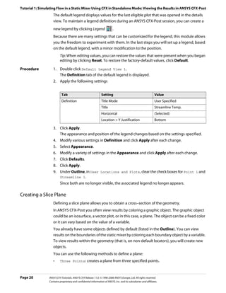
Next you will visualize how the expressions have scheduled the concentration of smoke
issued from the vent.
ANSYS CFX Tutorials. ANSYS CFX Release 11.0. © 1996-2006 ANSYS Europe, Ltd. All rights reserved. Page 101
Contains proprietary and confidential information of ANSYS, Inc. and its subsidiaries and affiliates.](https://image.slidesharecdn.com/ansys11tutorial-111218135319-phpapp01/85/Ansys-11-tutorial-113-320.jpg)
![Tutorial 4: Flow from a Circular Vent: Defining a Transient Simulation in ANSYS CFX-Pre
Plotting Smoke 1. Double-click ExpFunction in the Expressions tree view.
Concentration 2. Apply the following settings
Tab Setting Value
Plot t (Selected)
Start of Range 0 [s]
End of Range 30 [s]
3. Click Plot Expression.
The button name then changes to Define Plot, as shown.
As can be seen, the smoke concentration rises exponentially, and reaches 90% of its final
value at around 7 seconds.
4. Click the Boundary: Vent tab.
In the next step, you will apply the expression ExpFunction to the additional variable
smoke as it applies to the boundary Vent.
5. Apply the following settings
Tab Setting Value
Boundary Details Additional Variables > smoke > Option Value
Additional Variables > smoke > Value* ExpFunction
*. Click Enter Expression to enter text.
6. Click OK.
Page 102 ANSYS CFX Tutorials. ANSYS CFX Release 11.0. © 1996-2006 ANSYS Europe, Ltd. All rights reserved.
Contains proprietary and confidential information of ANSYS, Inc. and its subsidiaries and affiliates.](https://image.slidesharecdn.com/ansys11tutorial-111218135319-phpapp01/85/Ansys-11-tutorial-114-320.jpg)
![Tutorial 4: Flow from a Circular Vent: Defining a Transient Simulation in ANSYS CFX-Pre
Initialization Values
The steady state solution that you have finished calculating is used to supply the initial
values to the ANSYS CFX-Solver. You can leave all of the initialization data set to Automatic
and the initial values will be read automatically from the initial values file. Therefore, there
is no need to revisit the initialization tab.
Modifying the Solver Control
1. Click Solver Control .
2. Set Convergence Control > Max. Coeff. Loops to 3.
3. Leave the other settings at their default values.
4. Click OK to set the solver control parameters.
Output Control
To allow results to be viewed at different timesteps, it is necessary to create transient results
files at specified times. The transient results files do not have to contain all solution data. In
this step, you will create minimal transient results files.
To Create 1. From the main menu, select Insert > Solver > Output Control.
Minimal 2. Click the Trn Results tab.
Transient
Results Files 3. Click Add new item and then click OK to accept the default name for the object.
This creates a new transient results object. Each object can result in the production of
many transient results files.
4. Apply the following settings to Transient Results 1
Setting Value
Option Selected Variables
Output Variables List* Pressure, Velocity, smoke
Output Frequency > Option Time List
Output Frequency > Time List† 1, 2 , 3 [s]
*. Click the ellipsis icon to select items if they do not appear in the drop-down list. Use
the <Ctrl> key to select multiple items.
†. Do NOT click Enter Expression to enter lists of values. Enter the list without the
units, then set the units in the drop-down list.
5. Click Apply.
6. Create a second item with the default name Transient Results 2 and apply the
following settings to that item
Setting Value
Option Selected Variables
Output Variables List Pressure, Velocity, smoke
ANSYS CFX Tutorials. ANSYS CFX Release 11.0. © 1996-2006 ANSYS Europe, Ltd. All rights reserved. Page 103
Contains proprietary and confidential information of ANSYS, Inc. and its subsidiaries and affiliates.](https://image.slidesharecdn.com/ansys11tutorial-111218135319-phpapp01/85/Ansys-11-tutorial-115-320.jpg)
![Tutorial 4: Flow from a Circular Vent: Obtaining a Solution to the Transient Problem
Setting Value
Output Frequency > Option Time Interval
Output Frequency > Time Interval* 4 [s]
*. A transient results file will be produced every 4 s (including 0 s) and at 1 s, 2 s and
3 s. The files will contain no mesh and data for only the three selected variables. This
reduces the size of the minimal results files. A full results file is always written at the
end of the run.
7. Click OK.
Writing the Solver (.def) File
1. Click Write Solver File .
2. Apply the following settings
Setting Value
File name CircVent.def
Quit CFX–Pre * Select
*. If using ANSYS CFX-Pre in Standalone Mode.
3. Ensure Start Solver Manager is selected and click Save.
4. Quit ANSYS CFX-Pre, saving the simulation (.cfx) file at your discretion.
Obtaining a Solution to the Transient Problem
In this tutorial the ANSYS CFX-Solver will read the initial values for the problem from a file.
For details, see Initialization Values (p. 103). You need to specify the file name.
Define Run will be displayed when the ANSYS CFX-Solver Manager launches. Definition
File will already be set to the name of the definition file just written.
Notice that the text output generated by the ANSYS CFX-Solver will be more than you have
seen for steady-state problems. This is because each timestep consists of several inner
(coefficient) iterations. At the end of each timestep, information about various quantities is
printed to the text output area.
The variable smoke is now plotted under the Additional Variables tab.
1. Under Initial Values File, click Browse .
2. Select CircVentIni_001.res, which is the results file of the steady-state problem with
no smoke issuing from the chimney. If you have not run the first part of this tutorial, copy
CircVentIni_001.res from the <CFXROOT>/examples/ directory to your working
directory.
3. Click Open.
4. Click Start Run.
5. You may see a notice that the mesh from the initial values file will be used. This mesh is
the same as in the definition file. Click OK to continue.
Page 104 ANSYS CFX Tutorials. ANSYS CFX Release 11.0. © 1996-2006 ANSYS Europe, Ltd. All rights reserved.
Contains proprietary and confidential information of ANSYS, Inc. and its subsidiaries and affiliates.](https://image.slidesharecdn.com/ansys11tutorial-111218135319-phpapp01/85/Ansys-11-tutorial-116-320.jpg)
![Tutorial 4: Flow from a Circular Vent: Viewing the Results in ANSYS CFX-Post
ANSYS CFX-Solver runs and attempts to obtain a solution. This can take a long time
depending on your system. Eventually a dialog box is displayed.
6. When ANSYS CFX-Solver has finished, click Yes to post-process the results.
7. If using Standalone Mode, quit ANSYS CFX-Solver Manager.
Viewing the Results in ANSYS CFX-Post
In this tutorial, you will view the dispersion of smoke from the vent over time. When ANSYS
CFX-Post is loaded, the results that are immediately available are those at the final timestep;
in this case, at t = 30 s (this is nominally designated Final State).
Creating an Isosurface
An isosurface is a surface of constant value of a variable. For instance, it could be a surface
consisting of all points where the velocity is 1 [m s^-1]. In this case, you are going to create
an isosurface of smoke density (smoke is the additional variable that you specified earlier).
1. Right-click on a blank area in the viewer and select Predefined Camera > Isometric
View (Z up).
This ensures that the view is set to a position that is best suited to display the results.
2. From the main menu, select Insert > Location > Isosurface or under Location, click
Isosurface.
3. Click OK.
4. Apply the following settings
Tab Setting Value
Geometry Variable smoke
Value 0.005 [kg m^-3]
5. Click Apply.
• A bumpy surface will be displayed, showing the smoke starting to emerge from the
vent.
• The surface is rough because the mesh is coarse. For a smoother surface, you would
re-run the problem with a smaller mesh length scale.
• The surface will be a constant color as the default settings on the Color tab were
used.
• When Color Mode is set to either Constant or Use Plot Variable for an
isosurface, it appears as one color.
6. In Geometry, experiment by changing the Value so that you can see the shape of the
plume more clearly.
Zoom in and rotate the geometry, as required.
7. When you have finished, set the Value to 0.002 [kg m^-3].
8. Right-click on a blank spot in the viewer and select Predefined Camera > Isometric
View (Z up).
ANSYS CFX Tutorials. ANSYS CFX Release 11.0. © 1996-2006 ANSYS Europe, Ltd. All rights reserved. Page 105
Contains proprietary and confidential information of ANSYS, Inc. and its subsidiaries and affiliates.](https://image.slidesharecdn.com/ansys11tutorial-111218135319-phpapp01/85/Ansys-11-tutorial-117-320.jpg)
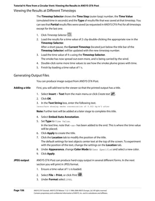
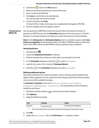
![Tutorial 5: Flow Around a Blunt Body: Defining a Simulation in ANSYS CFX-Pre
Setting Value
File name BluntBodyMesh.gtm
3. Click Open.
Creating the Domain
The flow in the domain is expected to be turbulent and approximately isothermal. The
Shear Stress Transport (SST) turbulence model with automatic wall function treatment will
be used because of its highly accurate predictions of flow separation. To take advantage of
the SST model, the boundary layer should be resolved with at least 10 mesh nodes. In order
to reduce computational time, the mesh in this tutorial is much coarser than that.
This tutorial uses an ideal gas as the fluid whereas previous tutorials have used a specific
fluid. When modeling a compressible flow using the ideal gas approximation to calculate
density variations, it is important to set a realistic reference pressure. This is because some
fluid properties depend on the absolute fluid pressure (calculated as the static pressure plus
the reference pressure).
1. Click Domain , and set the name to BluntBody.
2. Apply the following settings to BluntBody:
Tab Setting Value
General Options Basic Settings > Fluids List Air Ideal Gas
Domain Models > Pressure > Reference Pressure 1 [atm]
Fluid Models Heat Transfer > Option Isothermal
Heat Transfer > Fluid Temperature 288 [K]
Turbulence > Option Shear Stress Transport
3. Click OK.
Creating Composite Regions
An imported mesh may contain many 2D regions. For the purpose of creating boundary
conditions, it can sometimes be useful to group several 2D regions together and apply a
single boundary condition to the composite 2D region. In this case, you are going to create
a Union between two regions that both require a free slip wall boundary condition.
1. From the main menu, select Insert > Composite Region.
2. Set the name to FreeWalls and click OK.
3. Apply the following settings
Tab Setting Value
Basic Settings Dimension (Filter) 2D
4. In the region list, hold down the <Ctrl> key and select Free1 and Free2.
Page 112 ANSYS CFX Tutorials. ANSYS CFX Release 11.0. © 1996-2006 ANSYS Europe, Ltd. All rights reserved.
Contains proprietary and confidential information of ANSYS, Inc. and its subsidiaries and affiliates.](https://image.slidesharecdn.com/ansys11tutorial-111218135319-phpapp01/85/Ansys-11-tutorial-124-320.jpg)
![Tutorial 5: Flow Around a Blunt Body: Defining a Simulation in ANSYS CFX-Pre
5. Click OK.
Creating the Boundary Conditions
The simulation requires inlet, outlet, wall (no slip and free slip) and symmetry plane
boundary conditions. The regions for these boundary conditions were defined when the
mesh was created (except for the composite region just created for the free slip wall
boundary condition).
Inlet Boundary 1. Click Boundary Condition .
2. Under Name, type Inlet.
3. Apply the following settings
Tab Setting Value
Basic Settings Boundary Type Inlet
Location Inlet
Boundary Details Flow Regime > Option Subsonic
Mass and Momentum > Option Normal Speed
Mass and Momentum > Normal Speed 15 [m s^-1]
Turbulence > Option Intensity and Length Scale
Turbulence > Eddy Len. Scale 0.1 [m]
4. Click OK.
Outlet 1. Create a new boundary condition named Outlet.
Boundary 2. Apply the following settings
Tab Setting Value
Basic Settings Boundary Type Outlet
Location Outlet
Boundary Details Mass and Momentum > Option Static Pressure
Mass and Momentum > Relative Pressure 0 [Pa]
3. Click OK.
Free Slip Wall The top and side surfaces of the rectangular region will use free slip wall boundary
Boundary conditions.
• On free slip walls the shear stress is set to zero so that the fluid is not retarded.
• The velocity normal to the wall is also set to zero.
• The velocity parallel to the wall is calculated during the solution.
This is not an ideal boundary condition for this situation since the flow around the body will
be affected by the close proximity to the walls. If this case was modeling a wind tunnel
experiment, the domain should model the size and shape of the wind tunnel and use no-slip
walls. If this case was modeling a blunt body open to the atmosphere, a much larger domain
should be used to minimize the effect of the walls.
ANSYS CFX Tutorials. ANSYS CFX Release 11.0. © 1996-2006 ANSYS Europe, Ltd. All rights reserved. Page 113
Contains proprietary and confidential information of ANSYS, Inc. and its subsidiaries and affiliates.](https://image.slidesharecdn.com/ansys11tutorial-111218135319-phpapp01/85/Ansys-11-tutorial-125-320.jpg)
![Tutorial 5: Flow Around a Blunt Body: Defining a Simulation in ANSYS CFX-Pre
Tab Setting Value
Global Settings Initial Conditions > Cartesian Velocity Automatic with Value
Components > Option
Initial Conditions > Cartesian Velocity 15 [m s^-1]
Components > U
Initial Conditions > Cartesian Velocity 0 [m s^-1]
Components > V
Initial Conditions > Cartesian Velocity 0 [m s^-1]
Components > W
Initial Conditions > Turbulence Eddy (Selected)
Dissipation
3. Click OK.
Setting Solver Control
1. Click Solver Control .
2. Apply the following settings:
Tab Setting Value
Basic Settings Convergence Control > Max. Iterations 60
Convergence Control > Fluid Timescale Control > Physical Timescale
Timescale Control
Convergence Control > Fluid Timescale Control > 2 [s]
Physical Timescale
Convergence Criteria > Residual Target 1e-05
3. Click OK.
Writing the Solver (.def) File
1. Click Write Solver File .
2. Apply the following settings:
Setting Value
File name BluntBody.def
Quit CFX–Pre* (Selected)
*. If using ANSYS CFX-Pre in Standalone Mode.
3. Ensure Start Solver Manager is selected and click Save.
4. If using Standalone Mode, quit ANSYS CFX-Pre, saving the simulation (.cfx) file at your
discretion.
ANSYS CFX Tutorials. ANSYS CFX Release 11.0. © 1996-2006 ANSYS Europe, Ltd. All rights reserved. Page 115
Contains proprietary and confidential information of ANSYS, Inc. and its subsidiaries and affiliates.](https://image.slidesharecdn.com/ansys11tutorial-111218135319-phpapp01/85/Ansys-11-tutorial-127-320.jpg)

![Tutorial 5: Flow Around a Blunt Body: Viewing the Results in ANSYS CFX-Post
Creating Vectors
You are now going to create a vector plot to show velocity vectors behind the blunt body.
You need to first create an object to act as a locator, which, in this case, will be a sampling
plane. Then, create the vector plot itself.
Creating the A sampling plane is a plane with evenly spaced sampling points on it.
Sampling Plane
1. Right-click a blank area in the viewer and select Predefined Camera > View Towards
+Y.
This ensures that the changes can be seen.
2. Create a new plane named Sample.
3. Apply the following settings:
Tab Setting Value
Geometry Definition > Method Point and Normal
Definition > Point 6, -0.001, 1
Definition > Normal 0, 1, 0
Plane Bounds > Type Rectangular
Plane Bounds > X Size 2.5 [m]
Plane Bounds > Y Size 2.5 [m]
Plane Type Sample
Plane Type > X Samples 20
Plane Type > Y Samples 20
Render Draw Faces (Cleared)
Draw Lines (Selected)
4. Click Apply.
You can zoom in on the sampling plane to see the location of the sampling points
(where lines intersect). There are a total of 400 (20 * 20) sampling points on the plane. A
vector can be created at each sampling point.
5. Hide the plane by clearing the visibility check box next to Sample.
Creating a 1. Click Vector and accept the default name.
Vector Plot 2. Apply the following settings:
Using Different
Sampling
Methods Tab Setting Value
Geometry Definition > Locations Sample
Definition > Sampling Vertex
Symbol Symbol Size 0.25
3. Click Apply.
4. Zoom until the vector plot is roughly the same size as the viewer.
You should be able to see a region of recirculation behind the blunt body.
ANSYS CFX Tutorials. ANSYS CFX Release 11.0. © 1996-2006 ANSYS Europe, Ltd. All rights reserved. Page 121
Contains proprietary and confidential information of ANSYS, Inc. and its subsidiaries and affiliates.](https://image.slidesharecdn.com/ansys11tutorial-111218135319-phpapp01/85/Ansys-11-tutorial-133-320.jpg)
![Tutorial 5: Flow Around a Blunt Body: Viewing the Results in ANSYS CFX-Post
Tab Setting Value
Geometry Definition > Method YZ Plane
X -0.1 [m]
4. Click Apply.
The plane appears just upstream of the blunt body.
5. Clear the visibility check box for the plane.
This hides the plane from view, although the plane still exists.
6. Click Streamline . and click OK to accept the default name.
7. Apply the following settings:
Tab Setting Value
Geometry Type Surface Streamline
Definition > Surfaces Body
Definition > Start From Locations
Definition > Locations Starter
Definition > Max Points 100
Definition > Direction Forward
8. Apply the following settings.
The surface streamlines appear on half of the surface of the blunt body. They start near
the upstream end because the starting points were formed by projecting nodes from
the plane to the blunt body.
Moving Objects
In ANSYS CFX-Post, you can reposition some locator objects directly in the viewer by using
the mouse.
1. Select the visibility check box for the plane named Starter.
2. Select the Single Select mouse pointer from the Selection Tools toolbar.
3. In the viewer, click the Starter plane to select it, then use the left mouse button to drag
it along the X axis.
Notice that the streamlines are redrawn as the plane moves.
Creating a Surface Plot of y+
The velocity next to a no-slip wall boundary changes rapidly from a value of zero at the wall
to the free stream value a short distance away from the wall. This layer of high velocity
gradient is known as the boundary layer. Many meshes are not fine enough near a wall to
accurately resolve the velocity profile in the boundary layer. Wall functions can be used in
these cases to apply an assumed functional shape of the velocity profile. Other grids are fine
enough that they do not require wall functions, and application of the latter has little effect.
ANSYS CFX Tutorials. ANSYS CFX Release 11.0. © 1996-2006 ANSYS Europe, Ltd. All rights reserved. Page 123
Contains proprietary and confidential information of ANSYS, Inc. and its subsidiaries and affiliates.](https://image.slidesharecdn.com/ansys11tutorial-111218135319-phpapp01/85/Ansys-11-tutorial-135-320.jpg)


![Tutorial 6: Buoyant Flow in a Partitioned Cavity: Defining a Simulation in ANSYS CFX-Pre
2. Apply the following settings
Setting Value
File type CFX-4
File name Buoyancy2D.geo*
*. This file is in your tutorial directory.
3. Click Open.
Simulation Type
The default units and coordinate frame settings are suitable for this tutorial, but the
simulation type needs to be set to transient.
You will notice physics validation messages as the case is set to Transient. These errors will
be fixed in the later part of the tutorial.
1. Click Simulation Type .
2. Apply the following settings
Tab Setting Value
Basic Settings Simulation Type > Option Transient
Simulation Type > Time Duration > 2 [s]
Total Time*
Simulation Type > Time Steps > 0.025 [s]
Timesteps†
Simulation Type > Initial Time > Time 0 [s]
*. This is the total duration, in real time, for the simulation
†. This is the interval from one step, in real time, to the next. The simulation will
continue, moving forward in time by 0.025 s, until the total time has been reached
3. Click OK.
Page 130 ANSYS CFX Tutorials. ANSYS CFX Release 11.0. © 1996-2006 ANSYS Europe, Ltd. All rights reserved.
Contains proprietary and confidential information of ANSYS, Inc. and its subsidiaries and affiliates.](https://image.slidesharecdn.com/ansys11tutorial-111218135319-phpapp01/85/Ansys-11-tutorial-142-320.jpg)
![Tutorial 6: Buoyant Flow in a Partitioned Cavity: Defining a Simulation in ANSYS CFX-Pre
Creating the Domain
gsin30
30
gcos30
g
y
x
30
You will model the cavity as if it were tilted at an angle of 30°. You can do this by specifying
horizontal and vertical components of the gravity vector, which are aligned with the default
coordinate axes, as shown in the diagram above.
To Create a New 1. Click Domain , and set the name to Buoyancy2D.
Domain 2. Apply the following settings to Buoyancy2D
Tab Setting Value
General Basic Settings > Fluids List Air at 25 C
Options Domain Models > Pressure > Reference Pressure 1 [atm]
Domain Models > Buoyancy > Option Buoyant
Domain Models > Buoyancy > Gravity X Dirn. -4.9 [m s^-2]
Domain Models > Buoyancy > Gravity Y Dirn. -8.5 [m s^-2]
Domain Models > Buoyancy > Gravity Z Dirn. 0.0 [m s^-2]*
Domain Models > Buoyancy > Buoy. Ref. Temp. 40 [C]†
Fluid Models Heat Transfer > Option Thermal Energy
Turbulence > Option None (Laminar)
*. This produces a gravity vector which simulates the tilt of the cavity
†. Do not forget to change the units. This is just an approximate representative
domain temperature.
Initialization will be set up using Global Initialization , so there is no need to visit the
Initialization tab.
3. Click OK.
ANSYS CFX Tutorials. ANSYS CFX Release 11.0. © 1996-2006 ANSYS Europe, Ltd. All rights reserved. Page 131
Contains proprietary and confidential information of ANSYS, Inc. and its subsidiaries and affiliates.](https://image.slidesharecdn.com/ansys11tutorial-111218135319-phpapp01/85/Ansys-11-tutorial-143-320.jpg)
![Tutorial 6: Buoyant Flow in a Partitioned Cavity: Defining a Simulation in ANSYS CFX-Pre
Creating the Boundary Conditions
Hot and Cold You will create a wall boundary condition with a fixed temperature of 75 C on the bottom
Wall Boundary surface of the cavity, as follows:
1. Create a new boundary condition named hot.
2. Apply the following settings
Tab Setting Value
Basic Settings Boundary Type Wall
Location WALLHOT
Boundary Heat Transfer > Option Temperature
Details
Heat Transfer > Fixed Temperature 75 [C]
3. Click OK.
4. Create a new boundary condition named cold.
5. Apply the following settings
Tab Setting Value
Basic Settings Boundary Type Wall
Location WALLCOLD
Boundary Heat Transfer > Option Temperature
Details Heat Transfer > Fixed Temperature 5 [C]
6. Click OK.
Symmetry Plane A single symmetry plane boundary condition can be used for the front and back of the
Boundary cavity.
1. Create a new boundary condition named SymP.
2. Apply the following settings
Tab Setting Value
Basic Settings Boundary Type Symmetry
Location SYMMET1, SYMMET2*
*. Use the <Ctrl> key to select more than one region.
3. Click OK.
The default adiabatic wall boundary condition will automatically be applied to the
remaining boundaries.
Setting Initial Values
You should set initial settings using the Automatic with Value option when defining a
transient simulation. Using this option, the first run will use the specified initial conditions
while subsequent runs will use results file data for initial conditions.
Page 132 ANSYS CFX Tutorials. ANSYS CFX Release 11.0. © 1996-2006 ANSYS Europe, Ltd. All rights reserved.
Contains proprietary and confidential information of ANSYS, Inc. and its subsidiaries and affiliates.](https://image.slidesharecdn.com/ansys11tutorial-111218135319-phpapp01/85/Ansys-11-tutorial-144-320.jpg)
![Tutorial 6: Buoyant Flow in a Partitioned Cavity: Defining a Simulation in ANSYS CFX-Pre
1. Click Global Initialization .
2. Apply the following settings
Tab Setting Value
Global Settings Initial Conditions > Cartesian Velocity Automatic with
Components > Option Value
Initial Conditions > Cartesian Velocity 0 [m s^-1]
Components > U
Initial Conditions > Cartesian Velocity 0 [m s^-1]
Components > V
Initial Conditions > Cartesian Velocity 0 [m s^-1]
Components > W
Initial Conditions > Static Pressure > Relative 0 [Pa]
Pressure
Initial Conditions > Temperature > Temperature 5 [C]
3. Click OK.
Setting Output Control
1. Click Output Control .
2. Click the Trn Results tab.
3. Create a new Transient Results item with the default name.
4. Apply the following settings
Tab Setting Value
Trn Results Transient Results > Transient Results 1 > Selected Variables
Option
Transient Results > Transient Results 1 > Pressure, Temperature,
Output Variables List* Velocity
Transient Results > Transient Results 1 > Time Interval
Output Frequency > Option
Transient Results > Transient Results 1 > 0.1 [s]
Output Frequency > Time Interval
*. Click the ellipsis icon to select items if they do not appear in the drop-down list. Use
the <Ctrl> key to select multiple items.
5. Click OK.
Setting Solver Control
1. Click Solver Control .
2. Apply the following settings
ANSYS CFX Tutorials. ANSYS CFX Release 11.0. © 1996-2006 ANSYS Europe, Ltd. All rights reserved. Page 133
Contains proprietary and confidential information of ANSYS, Inc. and its subsidiaries and affiliates.](https://image.slidesharecdn.com/ansys11tutorial-111218135319-phpapp01/85/Ansys-11-tutorial-145-320.jpg)
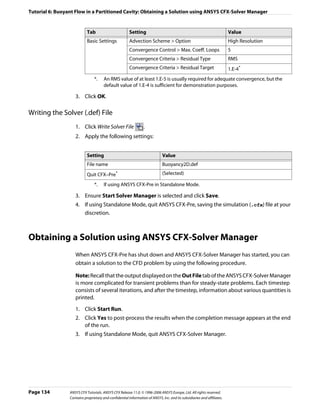
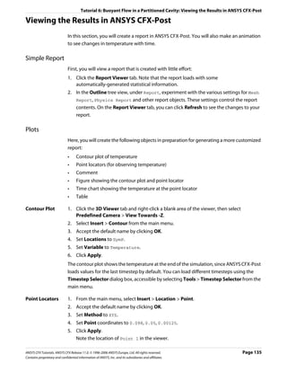
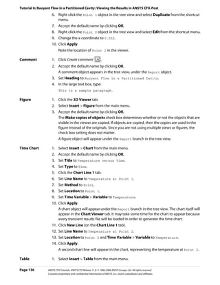
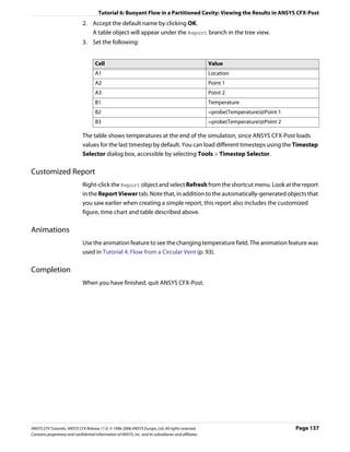

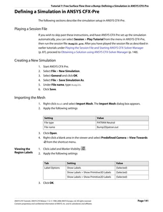
![Tutorial 7: Free Surface Flow Over a Bump: Defining a Simulation in ANSYS CFX-Pre
Creating Expressions for Initial and Boundary Conditions
Simulation of free surface flows usually requires defining boundary and initial conditions to
set up appropriate pressure and volume fraction fields. You will need to create expressions
using CEL (CFX Expression Language) to define these conditions.
In this simulation, the following conditions are set and require expressions:
• An inlet boundary where the volume fraction above the free surface is 1 for air and 0 for
water, and below the free surface is 0 for air and 1 for water.
• A pressure-specified outlet boundary, where the pressure above the free surface is
constant and the pressure below the free surface is a hydrostatic distribution. This
requires you to know the approximate height of the fluid at the outlet. In this case, an
analytical solution for 1D flow over a bump was used. The simulation is not sensitive to
the exact outlet fluid height, so an approximation is sufficient. You will examine the
effect of the outlet boundary condition in the post-processing section and confirm that
it does not affect the validity of the results. It is necessary to specify such a boundary
condition to force the flow downstream of the bump into the supercritical regime.
• An initial pressure field for the domain with a similar pressure distribution to that of the
outlet boundary.
Either create expressions using the Expressions workspace or import expressions from a
file.
• Creating Expressions (p. 142)
• Reading Expressions From a File (p. 143)
Creating 1. Right-click Expressions in the tree view and select Insert > Expression.
Expressions 2. Set the name to UpH and click OK.
3. Set Definition to 0.069 [m], and then click Apply.
4. Use the same method to create the expressions listed in the table below. These are
expressions for the downstream free surface height, the density of the fluid, the
upstream volume fractions of air and water, the upstream pressure distribution, the
downstream volume fractions of air and water, and the downstream pressure
distribution.
Name Definition
DownH 0.022 [m]
DenH 998 [kg m^-3]
UpVFAir step((y-UpH)/1[m])
UpVFWater 1-UpVFAir
UpPres DenH*g*UpVFWater*(UpH-y)
DownVFAir step((y-DownH)/1[m])
DownVFWater 1-DownVFAir
DownPres DenH*g*DownVFWater*(DownH-y)
5. Proceed to Creating the Domain (p. 143).
Page 142 ANSYS CFX Tutorials. ANSYS CFX Release 11.0. © 1996-2006 ANSYS Europe, Ltd. All rights reserved.
Contains proprietary and confidential information of ANSYS, Inc. and its subsidiaries and affiliates.](https://image.slidesharecdn.com/ansys11tutorial-111218135319-phpapp01/85/Ansys-11-tutorial-154-320.jpg)
![Tutorial 7: Free Surface Flow Over a Bump: Defining a Simulation in ANSYS CFX-Pre
Reading 1. Copy the file Bump2DExpressions.ccl to your working directory from the ANSYS CFX
Expressions examples directory.
From a File 2. Select File > Import CCL.
3. When Import CCL appears, ensure that Append is selected.
4. Select Bump2DExpressions.ccl.
5. Click Open.
6. After the file has been imported, use the Expression tree view to view the expressions
that have been created.
Creating the Domain
1. Right click Simulation in the Outline tree view and ensure that Automatic Default
Domain is selected. A domain named Default Domain should now appear under the
Simulation branch.
2. Double click Default Domain and apply the following settings
Tab Setting Value
General Basic Settings > Fluids List Air at 25 C, Water
Options Domain Models > Pressure > Reference Pressure 1 [atm]
Domain Models > Buoyancy > Option Buoyant
Domain Models > Buoyancy > Gravity X Dirn. 0 [m s^-2]
Domain Models > Buoyancy > Gravity Y Dirn.* -g
Domain Models > Buoyancy > Gravity Z Dirn. 0 [m s^-2]
Domain Models > Buoyancy > Buoy. Ref. Density† 1.185 [kg m^-3]
Domain Models > Buoyancy > Ref Location > Option Automatic
Fluid Models Multiphase Options > Homogeneous Model‡ (Selected)
Multiphase Options > Free Surface Model > Option Standard
Heat Transfer > Option Isothermal
Heat Transfer > Fluid Temperature 25 C
Turbulence > Option k-Epsilon
*. You need to click Enter Expression beside the field first.
†. Always set Buoyancy Reference Density to the density of the least dense fluid in free
surface calculations.
‡. The homogeneous model solves for a single solution field. This is only appropriate
in some simulations.
3. Click OK.
Creating the Boundary Conditions
Inlet Boundary 1. Create a new boundary condition named inflow.
2. Apply the following settings
ANSYS CFX Tutorials. ANSYS CFX Release 11.0. © 1996-2006 ANSYS Europe, Ltd. All rights reserved. Page 143
Contains proprietary and confidential information of ANSYS, Inc. and its subsidiaries and affiliates.](https://image.slidesharecdn.com/ansys11tutorial-111218135319-phpapp01/85/Ansys-11-tutorial-155-320.jpg)
![Tutorial 7: Free Surface Flow Over a Bump: Defining a Simulation in ANSYS CFX-Pre
Tab Setting Value
Basic Boundary Type Inlet
Settings
Location INFLOW
Boundary Mass and Momentum > Option Normal Speed
Details
Mass and Momentum > Option > Normal Speed 0.26 [m s^-1]
Turbulence > Option Intensity and Length Scale
Turbulence > Value 0.05
Turbulence > Eddy Len. Scale* UpH
Fluid Values Boundary Conditions Air as 25 C
Air at 25 C > Volume Fraction > Volume Fraction UpVFAir
Boundary Conditions Water
Water > Volume Fraction > Volume Fraction UpVFWater
*. Click the Enter Expression icon.
3. Click OK.
Outlet 1. Create a new boundary condition named outflow.
Boundary 2. Apply the following settings
Tab Setting Value
Basic Boundary Type Outlet
Settings Location OUTFLOW
Boundary Flow Regime> Option Subsonic
Details Mass and Momentum > Option Static Pressure
Mass and Momentum > Relative Pressure DownPres
3. Click OK.
Symmetry 1. Create a new boundary condition named front.
Boundary 2. Apply the following settings
Tab Setting Value
Basic Boundary Type Symmetry
Settings
Location FRONT
3. Click OK.
4. Create a new boundary condition named back.
5. Apply the following settings
Tab Setting Value
Basic Boundary Type Symmetry
Settings
Location BACK
Page 144 ANSYS CFX Tutorials. ANSYS CFX Release 11.0. © 1996-2006 ANSYS Europe, Ltd. All rights reserved.
Contains proprietary and confidential information of ANSYS, Inc. and its subsidiaries and affiliates.](https://image.slidesharecdn.com/ansys11tutorial-111218135319-phpapp01/85/Ansys-11-tutorial-156-320.jpg)
![Tutorial 7: Free Surface Flow Over a Bump: Defining a Simulation in ANSYS CFX-Pre
6. Click OK.
Wall and 1. Create a new boundary condition named top.
Opening 2. Apply the following settings
Boundaries
Tab Setting Value
Basic Settings Boundary Type Opening
Location TOP
Boundary Details Mass And Momentum > Option Static Pres. (Entrain)
Mass And Momentum > Relative Pressure 0 [Pa]
Turbulence > Option Zero Gradient
Fluid Values Boundary Conditions Air at 25 C
Boundary Conditions > Air at 25 C > 1.0
Volume Fraction > Volume Fraction
Boundary Conditions Water
Boundary Conditions > Water > Volume 0.0
Fraction > Volume Fraction
3. Click OK.
4. Create a new boundary condition named bottom.
5. Apply the following settings
Tab Setting Value
Basic Boundary Type Wall
Settings Location BOTTOM1, BOTTOM2, BOTTOM3
Boundary Wall Influence on Flow > Option No Slip
Details Wall Roughness > Option Smooth Wall
6. Click OK.
Setting Initial Values
1. Click Global Initialization .
2. Apply the following settings
ANSYS CFX Tutorials. ANSYS CFX Release 11.0. © 1996-2006 ANSYS Europe, Ltd. All rights reserved. Page 145
Contains proprietary and confidential information of ANSYS, Inc. and its subsidiaries and affiliates.](https://image.slidesharecdn.com/ansys11tutorial-111218135319-phpapp01/85/Ansys-11-tutorial-157-320.jpg)
![Tutorial 7: Free Surface Flow Over a Bump: Defining a Simulation in ANSYS CFX-Pre
Tab Setting Value
Global Settings Initial Conditions > Cartesian Velocity Automatic with Value
Components > Option
Initial Conditions > Cartesian Velocity 0.26 [m s^-1]
Components > U
Initial Conditions > Cartesian Velocity 0 [m s^-1]
Components > V
Initial Conditions > Cartesian Velocity 0 [m s^-1]
Components > W
Initial Conditions > Static Pressure > Option Automatic with Value
Initial Conditions > Static Pressure > Relative UpPres
Pressure
Initial Conditions > Turbulence Eddy Dissipation (Selected)
Fluid Settings Fluid Specific Initialization > Air at 25 C (Selected)
Air at 25 C > Initial Conditions > Volume Fraction > Automatic with Value
Option
Air at 25 C > Initial Conditions > Volume Fraction > UpVFAir
Volume Fraction
Fluid Settings Fluid Specific Initialization > Water (Selected)
Fluid Specific Initialization > Water > Initial Automatic with Value
Conditions > Volume Fraction > Option
Fluid Specific Initialization > Water > Initial UpVFWater
Conditions > Volume Fraction > Volume Fraction
3. Click OK.
Setting Mesh Adaption Parameters
1. Click Mesh Adaption .
2. Apply the following settings
Tab Setting Value
Basic Settings Activate Adaption (Selected)
Save Intermediate Files (Cleared)
Adaption Criteria > Variables List Air at 25 C.Volume Fraction
Adaption Criteria > Max. Num. Steps 2
Adaption Criteria > Option Multiple of Initial Mesh
Adaption Criteria > Node Factor 4
Adaption Convergence Criteria > Max. 100
Iter. per Step
Advanced Options Node Alloc. Param. 1.6
Number of Levels 2
3. Click OK.
Page 146 ANSYS CFX Tutorials. ANSYS CFX Release 11.0. © 1996-2006 ANSYS Europe, Ltd. All rights reserved.
Contains proprietary and confidential information of ANSYS, Inc. and its subsidiaries and affiliates.](https://image.slidesharecdn.com/ansys11tutorial-111218135319-phpapp01/85/Ansys-11-tutorial-158-320.jpg)
![Tutorial 7: Free Surface Flow Over a Bump: Defining a Simulation in ANSYS CFX-Pre
Setting Solver Control
Important: Setting Max Iterations to 200 and Number of Adaption Levels to 2 with a
maximum of 100 timesteps each, results in a total maximum number of timesteps of 400
(2*100+200=400).
1. Click Solver Control .
2. Apply the following settings
Tab Setting Value
Basic Settings Convergence Control > Max. Iterations 200
Convergence Control >Fluid Timescale Physical Timescale
Control > Timescale Control
Convergence Control >Fluid Timescale 0.25 [s]
Control > Physical Timescale
Advanced Options Multiphase Control (Selected)
Multiphase Control > Volume Fraction (Selected)
Coupling
Multiphase Control > Volume Fraction Coupled
Coupling > Option
Note: The options selected above activate the Coupled Volume Fraction solution algorithm.
This algorithm typically converges better than the Segregated Volume Faction algorithm for
buoyancy-driven problems such as this tutorial, which requires a 0.05 [s] timescale using the
Segregated Volume Faction algorithm compared with 0.25 [s] for the Coupled Volume
Fraction algorithm.
Note:
3. Click OK.
Writing the Solver (.def) File
1. Click Write Solver File .
2. Apply the following settings:
Setting Value
File name Bump2D.def
Quit CFX–Pre* (Selected)
*. If using ANSYS CFX-Pre in Standalone Mode.
3. Ensure Start Solver Manager is selected and click Save.
4. If using Standalone Mode, quit ANSYS CFX-Pre, saving the simulation (.cfx) file at your
discretion.
ANSYS CFX Tutorials. ANSYS CFX Release 11.0. © 1996-2006 ANSYS Europe, Ltd. All rights reserved. Page 147
Contains proprietary and confidential information of ANSYS, Inc. and its subsidiaries and affiliates.](https://image.slidesharecdn.com/ansys11tutorial-111218135319-phpapp01/85/Ansys-11-tutorial-159-320.jpg)
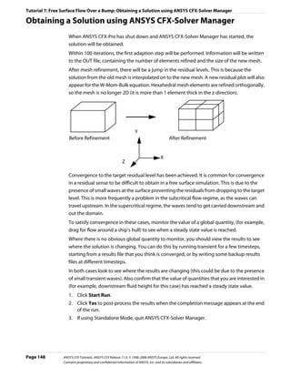
![Tutorial 7: Free Surface Flow Over a Bump: Viewing the Results in ANSYS CFX-Post
Viewing the Results in ANSYS CFX-Post
1. Select View Towards -Z by right-clicking on a blank area in the viewer and selecting
Predefined Camera > View Towards -Z.
2. Zoom in so the geometry fills the Viewer.
3. In the tree view under Bump2D, edit front.
4. Apply the following settings
Tab Setting Value
Color Mode Variable
Variable Water.Volume Fraction
5. Click Apply.
6. Clear the check box next to front.
Creating Velocity Vector Plots
The next step involves creating a sampling plane to display velocity vectors for Water.
1. Create a new plane named Plane 1.
2. Apply the following settings
Tab Setting Value
Geometry Definition > Method XY Plane
Plane Bounds > Type Rectangular
Plane Bounds > X Size 1.25 [m]
Plane Bounds > Y Size 0.3 [m]
Plane Bounds > X Angle 0 [degree]
Plane Type Sample
X Samples 160
Y Samples 40
Render Draw Faces (Cleared)
Draw Lines (Selected)
3. Click Apply.
4. Clear the check box next to Plane 1.
5. Create a new vector named Vector 1.
6. Apply the following settings
Tab Setting Value
Geometry Definition > Locations Plane 1
Definition > Variable * Water.Velocity
Symbol Symbol Size 0.5
ANSYS CFX Tutorials. ANSYS CFX Release 11.0. © 1996-2006 ANSYS Europe, Ltd. All rights reserved. Page 149
Contains proprietary and confidential information of ANSYS, Inc. and its subsidiaries and affiliates.](https://image.slidesharecdn.com/ansys11tutorial-111218135319-phpapp01/85/Ansys-11-tutorial-161-320.jpg)


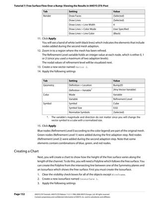
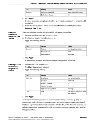
![Tutorial 7: Free Surface Flow Over a Bump: Using a Supercritical Outlet Condition
The chart shows a wiggle in the elevation of the free surface interface at the inlet. This is
related to an overspecification of conditions at the inlet, since both the inlet velocity and
elevation were specified. For a subcritical inlet, only the velocity or the total energy should
be specified. The wiggle is due to a small inconsistency between the specified elevation and
the elevation computed by the solver to obtain critical conditions at the bump. The wiggle
is analogous to one found if pressure and velocity were both specified at a subsonic inlet, in
a converging-diverging nozzle with choked flow at the throat.
Further Post-processing
You may wish to create some plots using the <Fluid>.Superficial Velocity variables.
This is the fluid volume fraction multiplied by the fluid velocity and is sometimes called the
volume flux. It is useful to use this variable for vector plots in separated multiphase flow, as
you will only see a vector where a significant amount of that phase exists.
Using a Supercritical Outlet Condition
For supercritical free surface flows, the supercritical outlet boundary condition is usually the
most appropriate boundary condition for the outlet, since it does not rely on the
specification of the outlet pressure distribution (which depends on an estimate of the free
surface height at the outlet). The supercritical outlet boundary condition requires a relative
pressure specification for the gas only; no pressure information is required for the liquid at
the outlet. For this tutorial, the relative gas pressure at the outlet should be set to 0 [Pa].
The supercritical outlet condition may admit multiple solutions. To find the supercritical
solution, it is often necessary to start with a static pressure outlet condition (as previously
done in this tutorial) or an average static pressure condition where the pressure is set
consistent with an elevation to drive the solution into the supercritical regime. The outlet
condition can then be changed to the supercritical option.
Page 154 ANSYS CFX Tutorials. ANSYS CFX Release 11.0. © 1996-2006 ANSYS Europe, Ltd. All rights reserved.
Contains proprietary and confidential information of ANSYS, Inc. and its subsidiaries and affiliates.](https://image.slidesharecdn.com/ansys11tutorial-111218135319-phpapp01/85/Ansys-11-tutorial-166-320.jpg)
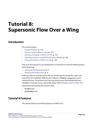
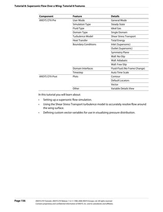
![Tutorial 8: Supersonic Flow Over a Wing: Overview of the Problem to Solve
Overview of the Problem to Solve
This example demonstrates the use of ANSYS CFX in simulating supersonic flow over a
symmetric NACA0012 airfoil at 0° angle of attack. A 2D section of the wing is modeled. A 2D
hexahedral mesh is provided that is imported into ANSYS CFX-Pre.
air speed 1.25 [m]
u = 600 m/s
outlet
30 [m]
wing surface
70 [m]
Defining a Simulation in ANSYS CFX-Pre
The following sections describe the simulation setup in ANSYS CFX-Pre.
Playing a Session File
If you wish to skip past these instructions, and have ANSYS CFX-Pre set up the simulation
automatically, you can select Session > Play Tutorial from the menu in ANSYS CFX-Pre,
then run the session file: WingSPS.pre. After you have played the session file as described
in earlier tutorials under Playing the Session File and Starting ANSYS CFX-Solver Manager
(p. 87), proceed to Obtaining a Solution using ANSYS CFX-Solver Manager (p. 162).
Creating a New Simulation
1. Start ANSYS CFX-Pre.
2. Select File > New Simulation.
3. Select General and click OK.
4. Select File > Save Simulation As.
5. Under File name, type WingSPS.
6. Click Save.
ANSYS CFX Tutorials. ANSYS CFX Release 11.0. © 1996-2006 ANSYS Europe, Ltd. All rights reserved. Page 157
Contains proprietary and confidential information of ANSYS, Inc. and its subsidiaries and affiliates.](https://image.slidesharecdn.com/ansys11tutorial-111218135319-phpapp01/85/Ansys-11-tutorial-169-320.jpg)
![Tutorial 8: Supersonic Flow Over a Wing: Defining a Simulation in ANSYS CFX-Pre
Importing the Mesh
1. Right-click Mesh and select Import Mesh. The Import Mesh dialog box appears.
2. Apply the following settings
Setting Value
File type PATRAN Neutral
File name WingSPSMesh.out
3. Click Open.
4. Right-click a blank area in the viewer and select Predefined Camera > Isometric View
(Y up) from the shortcut menu.
Creating the Domain
Creating a New 1. Right click Simulation in the Outline tree view and ensure that Automatic Default
Domain Domain is selected. A domain named Default Domain should now appear under the
Simulation branch.
2. Double click it and apply the following settings
Tab Setting Value
General Options Basic Settings > Location WING
Fluids List Air Ideal Gas
Domain Models > Pressure > 1 [atm]
Reference Pressure*
Fluid Models Heat Transfer > Option Total Energy†
Turbulence > Option Shear Stress Transport
*. When using an ideal gas, it is important to set an appropriate reference pressure
since some properties depend on the absolute pressure level.
†. The Total Energy model is appropriate for high speed flows since it includes kinetic
energy effects.
3. Click OK.
Creating the Boundary Conditions
Inlet Boundary 1. Create a new boundary condition named Inlet.
2. Apply the following settings
Tab Setting Value
Basic Settings Boundary Type Inlet
Location INLET
Page 158 ANSYS CFX Tutorials. ANSYS CFX Release 11.0. © 1996-2006 ANSYS Europe, Ltd. All rights reserved.
Contains proprietary and confidential information of ANSYS, Inc. and its subsidiaries and affiliates.](https://image.slidesharecdn.com/ansys11tutorial-111218135319-phpapp01/85/Ansys-11-tutorial-170-320.jpg)
![Tutorial 8: Supersonic Flow Over a Wing: Defining a Simulation in ANSYS CFX-Pre
Tab Setting Value
Boundary Details Flow Regime > Option Supersonic
Mass and Momentum > Option Cart. Vel. & Pressure
Mass and Momentum > U 600 [m s^-1]
Mass and Momentum > V 0 [m s^-1]
Mass and Momentum > W 0 [m s^-1]
Mass and Momentum > Rel. Static Pres. 0 [Pa]
Turbulence > Option Intensity and Length Scale
Turbulence > Value 0.01
Turbulence > Eddy Len. Scale 0.02 [m]
Heat Transfer > Static Temperature 300 [K]
3. Click OK.
Outlet 1. Create a new boundary condition named Outlet.
Boundary 2. Apply the following settings
Tab Setting Value
Basic Settings Boundary Type Outlet
Location OUTLET
Boundary Details Flow Regime > Option Supersonic
3. Click OK.
Symmetry Plane 1. Create a new boundary condition named SymP1.
Boundary 2. Apply the following settings
Tab Setting Value
Basic Settings Boundary Type Symmetry
Location SIDE1
3. Click OK.
4. Create a new boundary condition named SymP2.
5. Apply the following settings
Tab Setting Value
Basic Settings Boundary Type Symmetry
Location SIDE2
6. Click OK.
7. Create a new boundary condition named Bottom.
8. Apply the following settings
ANSYS CFX Tutorials. ANSYS CFX Release 11.0. © 1996-2006 ANSYS Europe, Ltd. All rights reserved. Page 159
Contains proprietary and confidential information of ANSYS, Inc. and its subsidiaries and affiliates.](https://image.slidesharecdn.com/ansys11tutorial-111218135319-phpapp01/85/Ansys-11-tutorial-171-320.jpg)
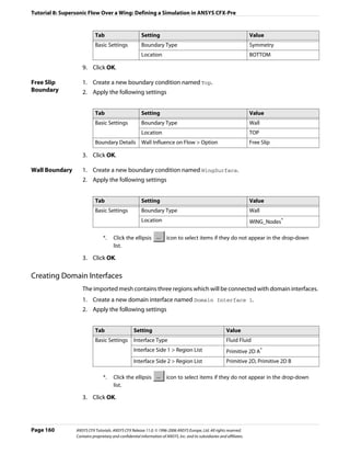
![Tutorial 8: Supersonic Flow Over a Wing: Defining a Simulation in ANSYS CFX-Pre
Setting Initial Values
For high speed compressible flow, the ANSYS CFX-Solver usually requires sensible initial
conditions to be set for the velocity field.
1. Click Global Initialization .
2. Apply the following settings
Tab Setting Value
Global Initial Conditions > Cartesian Velocity Components > Option Automatic
Settings with Value
Initial Conditions > Cartesian Velocity Components > U 600 [m s^-1]
Initial Conditions > Cartesian Velocity Components > V 0 [m s^-1]
Initial Conditions > Cartesian Velocity Components > W 0 [m s^-1]
Initial Conditions > Temperature > Option Automatic
with Value
Initial Conditions > Temperature > Temperature 300 [K]
Initial Conditions > Turbulence Eddy Dissipation (Selected)
3. Click OK.
Setting Solver Control
The residence time for the fluid is approximately:
70 [m] / 600 [m s^-1] = 0.117 [s]
In the next step, you will start with a conservative time scale that gradually increases
towards the fluid residence time as the residuals decrease. A user specified maximum time
scale can be combined with an auto timescale in ANSYS CFX-Pre.
1. Click Solver Control .
2. Apply the following settings
Tab Setting Value
Basic Settings Convergence Control > Fluid Timescale (Selected)
Control > Maximum Timescale
Convergence Control > Fluid Timescale 0.1 [s]
Control > Maximum Timescale > Maximum
Timescale
Convergence Criteria > Residual Target 1.0e-05
3. Click OK.
Writing the Solver (.def) File
Since this tutorial uses domain interfaces and the Summarize Interface Data toggle was
selected, an information window is displayed that informs you of the connection type used
for each domain interface.
ANSYS CFX Tutorials. ANSYS CFX Release 11.0. © 1996-2006 ANSYS Europe, Ltd. All rights reserved. Page 161
Contains proprietary and confidential information of ANSYS, Inc. and its subsidiaries and affiliates.](https://image.slidesharecdn.com/ansys11tutorial-111218135319-phpapp01/85/Ansys-11-tutorial-173-320.jpg)
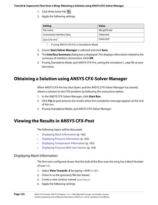

![Tutorial 8: Supersonic Flow Over a Wing: Viewing the Results in ANSYS CFX-Post
1. Create a new variable named Variable 1.
2. Apply the following settings
Name Setting Value
Variable 1 Vector (Selected)
X Expression (Pressure+101325[Pa])*Normal X
Y Expression (Pressure+101325[Pa])*Normal Y
Z Expression (Pressure+101325[Pa])*Normal Z
3. Click Apply.
4. Create a new vector named Vector 1.
5. Apply the following settings
Tab Setting Value
Geometry Locations WingSurface
Variable Variable 1
Symbol Symbol Size 0.04
6. Click Apply.
7. Zoom in on the wing in order to see the created vector plot.
Page 164 ANSYS CFX Tutorials. ANSYS CFX Release 11.0. © 1996-2006 ANSYS Europe, Ltd. All rights reserved.
Contains proprietary and confidential information of ANSYS, Inc. and its subsidiaries and affiliates.](https://image.slidesharecdn.com/ansys11tutorial-111218135319-phpapp01/85/Ansys-11-tutorial-176-320.jpg)
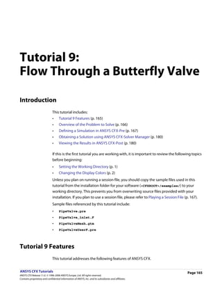
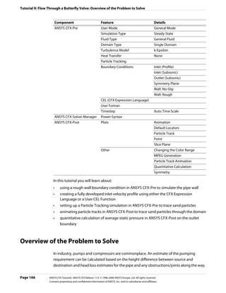
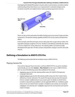
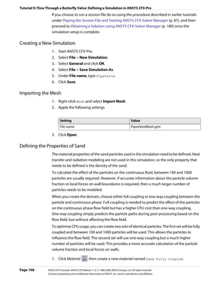
![Tutorial 9: Flow Through a Butterfly Valve: Defining a Simulation in ANSYS CFX-Pre
2. Apply the following settings:
Tab Setting Value
Basic Settings Material Group Particle Solids
Thermodynamic State (Selected)
Material Properties Thermodynamic Properties > Equation of 2300 [kg m^-3]
State > Density
Thermodynamic Properties >Specific Heat (Selected)
Capacity
Thermodynamic Properties >Specific Heat 0 [J kg^-1 K^-1]*
Capacity > Specific Heat Capacity
Thermodynamic Properties > Reference (Selected)
State
Thermodynamic Properties > Reference Specified Point
State > Option
Thermodynamic Properties > Reference 300 [K]
State > Ref. Temperature
*. This value is not used because heat transfer is not modeled in this tutorial.
3. Click OK.
4. Under Materials, right-click Sand Fully Coupled and select Duplicate from the
shortcut menu.
5. Name the duplicate Sand One Way Coupled.
6. Click OK.
Sand One Way Coupled is created with properties identical to Sand Fully Coupled.
Creating the Domain
1. Right click Simulation in the Outline tree view and ensure that Automatic Default
Domain is selected. A domain named Default Domain should now appear under the
Simulation branch.
2. Double click Default Domain and apply the following settings
Tab Setting Value
General Options Basic Settings > Fluids List Water
Basic Settings > Particle Tracking (Selected)
Basic Settings > Particle Tracking > Particles List Sand Fully Coupled,
Sand One Way Coupled
Domain Models > Pressure > Reference Pressure 1 [atm]
Fluid Models Heat Transfer > Option None
Turbulence > Option k-Epsilon*
ANSYS CFX Tutorials. ANSYS CFX Release 11.0. © 1996-2006 ANSYS Europe, Ltd. All rights reserved. Page 169
Contains proprietary and confidential information of ANSYS, Inc. and its subsidiaries and affiliates.](https://image.slidesharecdn.com/ansys11tutorial-111218135319-phpapp01/85/Ansys-11-tutorial-181-320.jpg)
![Tutorial 9: Flow Through a Butterfly Valve: Defining a Simulation in ANSYS CFX-Pre
Tab Setting Value
Fluid Details Sand Fully Coupled (Selected)
Sand Fully Coupled > Morphology > Option Solid Particles
Sand Fully Coupled > Morphology > Particle (Selected)
Diameter Distribution
Sand Fully Coupled > Morphology > Particle Normal in Diameter by
Diameter Distribution > Option Mass
Sand Fully Coupled > Morphology > Particle 50e-6 [m]
Diameter Distribution > Minimum Diameter
Sand Fully Coupled > Morphology > Particle 500e-6 [m]
Diameter Distribution > Maximum Diameter
Sand Fully Coupled > Morphology > Particle 250e-6 [m]
Diameter Distribution > Mean Diameter
Sand Fully Coupled > Morphology > Particle 70e-6 [m]
Diameter Distribution > Std. Deviation
Sand Fully Coupled > Erosion Model (Selected)
Sand Fully Coupled > Erosion Model > Option Finnie
Sand Fully Coupled > Erosion Model > Vel. 2.0
Power Factor
Sand Fully Coupled > Erosion Model > Reference 1 [m s^-1]
Velocity
*. The turbulence model only applies to the continuous phase and not the particle
phases.
3. Apply the following settings
Page 170 ANSYS CFX Tutorials. ANSYS CFX Release 11.0. © 1996-2006 ANSYS Europe, Ltd. All rights reserved.
Contains proprietary and confidential information of ANSYS, Inc. and its subsidiaries and affiliates.](https://image.slidesharecdn.com/ansys11tutorial-111218135319-phpapp01/85/Ansys-11-tutorial-182-320.jpg)
![Tutorial 9: Flow Through a Butterfly Valve: Defining a Simulation in ANSYS CFX-Pre
Tab Setting Value
Fluid Details Sand One Way Coupled (Selected)
Sand One Way Coupled > Morphology > Solid Particles
Option
Sand One Way Coupled > Morphology > (Selected)
Particle Diameter Distribution
Sand One Way Coupled > Morphology > Normal in Diameter by Mass
Particle Diameter Distribution > Option
Sand One Way Coupled > Morphology > 50e-6 [m]
Particle Diameter Distribution > Minimum
Diameter
Sand One Way Coupled > Morphology > 500e-6 [m]
Particle Diameter Distribution > Maximum
Diameter
Sand One Way Coupled > Morphology > 250e-6 [m]
Particle Diameter Distribution > Mean
Diameter
Sand One Way Coupled > Morphology > 70e-6 [m]
Particle Diameter Distribution > Std.
Deviation
Sand One Way Coupled > Erosion Model (Selected)
Sand One Way Coupled > Erosion Model > Finnie
Option
Sand One Way Coupled > Erosion Model > 2.0
Vel. Power Factor
Sand One Way Coupled > Erosion Model > 1 [m s^-1]
Reference Velocity
4. Apply the following settings
Tab Setting Value
Fluid Details Water (Selected)
Water > Morphology > Option Continuous Fluid
Fluid Pairs Fluid Pairs Water | Sand Fully
Coupled
Fluid Pairs > Water | Sand Fully Coupled > Fully Coupled
Particle Coupling
Fluid Pairs > Water | Sand Fully Coupled > Schiller Naumann
Momentum Transfer > Drag Force > Option
Fluid Pairs Water | Sand One Way
Coupled
Fluid Pairs > Water | Sand One Way Coupled > One-way Coupling
Particle Coupling
Fluid Pairs > Water | Sand One Way Coupled > Schiller Naumann
Momentum Transfer > Drag Force > Option
5. Click OK.
ANSYS CFX Tutorials. ANSYS CFX Release 11.0. © 1996-2006 ANSYS Europe, Ltd. All rights reserved. Page 171
Contains proprietary and confidential information of ANSYS, Inc. and its subsidiaries and affiliates.](https://image.slidesharecdn.com/ansys11tutorial-111218135319-phpapp01/85/Ansys-11-tutorial-183-320.jpg)
![Tutorial 9: Flow Through a Butterfly Valve: Defining a Simulation in ANSYS CFX-Pre
Creating the Inlet Velocity Profile
In previous tutorials you have often defined a uniform velocity profile at an inlet boundary.
This means that the inlet velocity near to the walls is the same as that at the center of the
inlet. If you look at the results from these simulations, you will see that downstream of the
inlet, a boundary layer will develop, so that the downstream near wall velocity is much lower
than the inlet near wall velocity.
You can simulate an inlet more accurately by defining an inlet velocity profile, so that the
boundary layer is already fully developed at the inlet. The one seventh power law will be
used in this tutorial to describe the profile at the pipe inlet. The equation for this is:
1
--
r 7
U = W max ⎛ 1 – ---------- ⎞
- (Eqn. 1)
⎝ R max⎠
where W max is the pipe centerline velocity, R max is the pipe radius, and r is the distance
from the pipe centerline.
A non uniform (profile) boundary condition can be created by:
• Creating an expression using CEL that describes the inlet profile.
OR
• Creating a User CEL Function which uses a user subroutine (linked to the ANSYS
CFX-Solver during execution) to describe the inlet profile.
OR
• Loading a BC profile file (a file which contains profile data).
Profiles created from data files are not used in this tutorial, but are used in the tutorial
Tutorial 3: Flow in a Process Injection Mixing Pipe (p. 77).
In this tutorial, you use one of the first two methods listed above to define the velocity
profile for the inlet boundary condition. The results from each method will be identical.
Using a CEL expression is the easiest way to create the profile. The User CEL Function
method is more complex but is provided as an example of how to use this feature. For more
complex profiles, it may be necessary to use a User CEL Function or a BC profile file.
To use the User CEL Function method, continue with this tutorial from User CEL Function
Method for the Inlet Velocity Profile (p. 173). Note that you will need access to a Fortran
compiler to be able to complete the tutorial by the User CEL Function method.
To use the expression method, continue with the tutorial from this point.
Expression 1. Create the following expressions.
Method for the
Inlet Velocity
Profile Name Definition
Rmax 20 [mm]
Wmax 5 [m s^-1]
Wprof Wmax*(abs(1-r/Rmax)^0.143)
Page 172 ANSYS CFX Tutorials. ANSYS CFX Release 11.0. © 1996-2006 ANSYS Europe, Ltd. All rights reserved.
Contains proprietary and confidential information of ANSYS, Inc. and its subsidiaries and affiliates.](https://image.slidesharecdn.com/ansys11tutorial-111218135319-phpapp01/85/Ansys-11-tutorial-184-320.jpg)
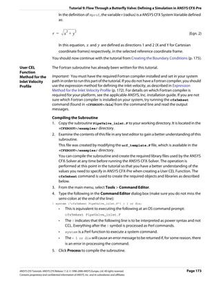
![Tutorial 9: Flow Through a Butterfly Valve: Defining a Simulation in ANSYS CFX-Pre
The output produced when this command is executed will be printed to your terminal
window.
Note: You can use the -double option (that is, cfx5mkext -double PipeValve_inlet.F)
to compile the subroutine for use with double precision.
A subdirectory will have been created in your working directory whose name is system
dependent (for example, on IRIX it is named irix). This subdirectory contains the
shared object library.
Note: If you are running problems in parallel over multiple platforms then you will need to
create these subdirectories using the cfx5mkext command for each different platform.
• You can view more details about the cfx5mkext command by running
cfx5mkext -help
• You can set a Library Name and Library Path using the -name and -dest options
respectively.
• If these are not specified, the default Library Name is that of your Fortran file and the
default Library Path is your current working directory.
6. Close the Command Editor dialog box.
Creating the Input Arguments
Next, you will create some values that will be used as input arguments when the subroutine
is called.
1. Click Expression .
2. Set Name to Wmax, and then click OK.
3. Type 5 [m s^-1] into the Definition box, and then click Apply.
The expression will be listed in the Expressions tree view.
4. Use the same method to create an expression named Rmax defined to be 20 [mm].
Creating the User CEL Function
Two steps are required to define a User CEL Function that uses the compiled Fortran
subroutine. First, a User Routine that points to the Fortran subroutine will be created. Then
a User CEL Function that points to the User Routine will be created.
1. From the main toolbar, click User Routine .
2. Set Name to WprofRoutine, and then click OK.
The User Routine details view appears.
3. Set Option to User CEL Function.
4. Set Calling Name to inlet_velocity.
• This is the name of the subroutine within the Fortran file.
• Always use lower case letters for the calling name, even if the subroutine name in
the Fortran file is in upper case.
5. Set Library Name to PipeValve_inlet.
• This is the name passed to the cfx5mkext command by the -name option.
• If the -name option is not specified, a default is used.
Page 174 ANSYS CFX Tutorials. ANSYS CFX Release 11.0. © 1996-2006 ANSYS Europe, Ltd. All rights reserved.
Contains proprietary and confidential information of ANSYS, Inc. and its subsidiaries and affiliates.](https://image.slidesharecdn.com/ansys11tutorial-111218135319-phpapp01/85/Ansys-11-tutorial-186-320.jpg)
![Tutorial 9: Flow Through a Butterfly Valve: Defining a Simulation in ANSYS CFX-Pre
• The default is the Fortran file name without the .F extension.
6. Set Library Path to the directory where the cfx5mkext command was executed
(usually the current working directory). For example:
• UNIX: /home/user/cfx/tutorials/PipeValve.
• Windows: c:usercfxtutorialsPipeValve.
This can be accomplished quickly by clicking Browse (next to Library Path),
browsing to the appropriate folder in Select Directory (not necessary if selecting
the working directory), and clicking OK (in Select Directory).
7. Click OK to complete the definition of the user routine.
8. Click User Function .
9. Set Name to WprofFunction, and then click OK.
The Function details view appears.
Important: You must not use the same name for the function and the routine.
10. Set Option to User Function.
11. Set User Routine Name to WprofRoutine.
12. Set Argument Units to [m s^-1], [m], [m]. These are the units for the three input
arguments: Wmax, r, and Rmax.
Set Result Units to [m s^-1], since the result will be a velocity for the inlet.
1. Click OK to complete the User Function specification.
You can now use the user function (WprofFunction) in place of a velocity value by
entering the expression WprofFunction(Wmax, r, Rmax) (although it only makes
sense for the W component of the inlet velocity in this tutorial).
In the definition of WprofFunction, the variable r (radius) is a system variable defined
as:
2 2
r = x +y (Eqn. 3)
In this equation, x and y are defined as directions 1 and 2 (X and Y for Cartesian
coordinate frames) respectively, in the selected reference coordinate frame.
Creating the Boundary Conditions
Inlet Boundary 1. Create a new boundary condition named inlet.
2. Apply the following settings
Tab Setting Value
Basic Settings Boundary Type Inlet
Location inlet
ANSYS CFX Tutorials. ANSYS CFX Release 11.0. © 1996-2006 ANSYS Europe, Ltd. All rights reserved. Page 175
Contains proprietary and confidential information of ANSYS, Inc. and its subsidiaries and affiliates.](https://image.slidesharecdn.com/ansys11tutorial-111218135319-phpapp01/85/Ansys-11-tutorial-187-320.jpg)
![Tutorial 9: Flow Through a Butterfly Valve: Defining a Simulation in ANSYS CFX-Pre
Tab Setting Value
Boundary Mass And Momentum > Option Cart. Vel. Components
Details Mass And Momentum > U 0 [m s^-1]
Mass And Momentum > V 0 [m s^-1]
Mass And Momentum > W Wprof -OR-
WprofFunction(Wmax,
r, Rmax)*
Fluid Values† Boundary Conditions Sand Fully Coupled
Sand Fully Coupled > Particle Behavior > Define (Selected)
Particle Behavior
Sand Fully Coupled > Mass and Momentum > Cart. Vel. Components‡
Option
Sand Fully Coupled > Mass And Momentum > U 0 [m s^-1]
Sand Fully Coupled > Mass And Momentum > V 0 [m s^-1]
Sand Fully Coupled > Mass And Momentum > W Wprof -OR-
WprofFunction(Wmax,
r, Rmax)**
Sand Fully Coupled > Particle Position > Option Uniform Injection
Sand Fully Coupled > Particle Position > Number Direct Specification
of Positions > Option
Sand Fully Coupled > Particle Position > Number 200
of Positions > Number
Sand Fully Coupled > Particle Mass Flow > Mass 0.01 [kg s^-1]
Flow Rate
Fluid Values Boundary Conditions Sand One Way Coupled
Sand One Way Coupled > Particle Behavior > (Selected)
Define Particle Behavior
Sand One Way Coupled > Mass and Momentum > Cart. Vel. Components††
Option
Sand One Way Coupled > Mass And Momentum > 0 [m s^-1]
U
Sand One Way Coupled > Mass And Momentum > 0 [m s^-1]
V
Sand One Way Coupled > Mass And Momentum > Wprof -OR-
W WprofFunction(Wmax,
r, Rmax)‡‡
Sand One Way Coupled > Particle Position > Uniform Injection
Option
Sand One Way Coupled > Particle Position > Direct Specification
Number of Positions > Option
Sand One Way Coupled > Particle Position > 5000
Number of Positions > Number
Sand One Way Coupled > Particle Position > 0.01 [kg s^-1]
Particle Mass Flow Rate > Mass Flow Rate
Page 176 ANSYS CFX Tutorials. ANSYS CFX Release 11.0. © 1996-2006 ANSYS Europe, Ltd. All rights reserved.
Contains proprietary and confidential information of ANSYS, Inc. and its subsidiaries and affiliates.](https://image.slidesharecdn.com/ansys11tutorial-111218135319-phpapp01/85/Ansys-11-tutorial-188-320.jpg)
![Tutorial 9: Flow Through a Butterfly Valve: Defining a Simulation in ANSYS CFX-Pre
*. Use the Expressions details view to enter either Wprof if using the expression
method, or WprofFunction(Wmax, r, Rmax) if using the User CEL Function
method.
†. Do NOT select Particle Diameter Distribution. The diameter distribution was
defined when creating the domain; this option would override those settings for
this boundary only.
‡. Instead of manually specifying the same velocity profile as the fluid, you can also
select the Zero Slip Velocity option.
**. as you did on the Boundary Details tab
††. Instead of manually specifying the same velocity profile as the fluid, you can also
select the Zero Slip Velocity option.
‡‡. as you did on the Boundary Details tab
3. Click OK.
One-way coupled particles are tracked as a function of the fluid flow field. The latter is not
influenced by the one-way coupled particles. The fluid flow will therefore be influenced by
the 0.01 [kg s^-1] flow of two-way coupled particles, but not by the 0.01 [kg s^-1] flow of
one-way coupled particles.
Outlet 1. Create a new boundary condition named outlet.
Boundary 2. Apply the following settings
Tab Setting Value
Basic Settings Boundary Type Outlet
Location outlet
Boundary Flow Regime > Option Subsonic
Details Mass and Momentum > Option Average Static Pressure
Mass and Momentum > Relative Pressure 0 [Pa]
3. Click OK.
Symmetry Plane 1. Create a new boundary condition named symP.
Boundary 2. Apply the following settings
Tab Setting Value
Basic Settings Boundary Type Symmetry
Location symP
3. Click OK.
Pipe Wall 1. Create a new boundary condition named pipe wall.
Boundary 2. Apply the following settings
Tab Setting Value
Basic Boundary Type Wall
Settings
Location pipe wall
ANSYS CFX Tutorials. ANSYS CFX Release 11.0. © 1996-2006 ANSYS Europe, Ltd. All rights reserved. Page 177
Contains proprietary and confidential information of ANSYS, Inc. and its subsidiaries and affiliates.](https://image.slidesharecdn.com/ansys11tutorial-111218135319-phpapp01/85/Ansys-11-tutorial-189-320.jpg)
![Tutorial 9: Flow Through a Butterfly Valve: Defining a Simulation in ANSYS CFX-Pre
Tab Setting Value
Boundary Wall Roughness > Option Rough Wall
Details Roughness Height 0.2 [mm]*
Fluid Boundary Conditions Sand Fully Coupled
Values Boundary Conditions > Sand Fully Coupled > Velocity Restitution Coefficient
> Option
Boundary Conditions > Sand Fully Coupled > Velocity 0.8
> Perpendicular Coeff.
Boundary Conditions > Sand Fully Coupled > Velocity 1
> Parallel Coeff.
Boundary Conditions Sand One Way Coupled
Boundary Conditions > Sand One Way Coupled > Restitution Coefficient
Velocity > Option
Boundary Conditions > Sand One Way Coupled > 0.8
Velocity > Perpendicular Coeff.
Boundary Conditions > Sand One Way Coupled > 1
Velocity > Parallel Coeff.
*. Make sure that you change the units to millimetres. The thickness of the first
element should be of the same order as the roughness height.
3. Click OK.
Editing the 1. In the Outline tree view, edit the boundary condition named Default Domain
Default Default.
Boundary 2. Apply the following settings
Condition
Tab Setting Value
Fluid Values Boundary Conditions Sand Fully Coupled
Boundary Conditions > Sand Fully 0.9
Coupled > Velocity > Perpendicular Coeff.
Boundary Conditions Sand One Way Coupled
Boundary Conditions > Sand One Way 0.9
Coupled > Velocity > Perpendicular Coeff.
3. Click OK.
Setting Initial Values
1. Click Global Initialization .
2. Apply the following settings
Page 178 ANSYS CFX Tutorials. ANSYS CFX Release 11.0. © 1996-2006 ANSYS Europe, Ltd. All rights reserved.
Contains proprietary and confidential information of ANSYS, Inc. and its subsidiaries and affiliates.](https://image.slidesharecdn.com/ansys11tutorial-111218135319-phpapp01/85/Ansys-11-tutorial-190-320.jpg)
![Tutorial 9: Flow Through a Butterfly Valve: Defining a Simulation in ANSYS CFX-Pre
Tab Setting Value
Global Settings Initial Conditions > Cartesian Velocity Automatic with Value
Components > Option
Initial Conditions > Cartesian Velocity 0 [m s^-1]
Components > Option > U
Initial Conditions > Cartesian Velocity 0 [m s^-1]
Components > Option > V
Initial Conditions > Cartesian Velocity Wprof -OR-
Components > Option > W WprofFunction(Wmax, r,
Rmax)*
Initial Conditions > Turbulence Eddy (Selected)
Dissipation
*. Use Enter Expression to enter Wprof if using the Expression method; enter
WprofFunction(Wmax, r, Rmax) if using the User CEL Function method.
3. Click OK.
Setting Solver Control
1. Click Solver Control .
2. Apply the following settings
Tab Setting Value
Basic Settings Advection Scheme > Option Specified Blend Factor
Advection Scheme > Blend Factor 0.75
Particle Control Particle Integration > Maximum Tracking Time (Selected)
Particle Integration > Maximum Tracking Time 10 [s]
> Value
Particle Integration > Maximum Tracking (Selected)
Distance
Particle Integration > Maximum Tracking 10 [m]
Distance > Value
Particle Integration > Max. Num. Integration (Selected)
Steps
Particle Integration > Max. Num. Integration 10000
Steps > Value
Particle Integration > Max. Particle Intg. Time (Selected)
Step
Particle Integration > Max. Particle Intg. Time 1e+10 [s]
Step > Value
3. Click OK.
ANSYS CFX Tutorials. ANSYS CFX Release 11.0. © 1996-2006 ANSYS Europe, Ltd. All rights reserved. Page 179
Contains proprietary and confidential information of ANSYS, Inc. and its subsidiaries and affiliates.](https://image.slidesharecdn.com/ansys11tutorial-111218135319-phpapp01/85/Ansys-11-tutorial-191-320.jpg)

![Tutorial 9: Flow Through a Butterfly Valve: Viewing the Results in ANSYS CFX-Post
Tab Setting Value
Color Mode Variable
Variable Sand One Way Coupled.Erosion Rate Density*
Range User Specified
Min 0 [kg m^-2 s^-1]
Max 25 [kg m^-2 s^-1]†
*. This is statistically better than Sand Fully Coupled.Erosion Rate Density since
many more particles were calculated for Sand One Way Coupled.
†. This range is used to gain a better resolution of the wall shear stress values around
the edge of the valve surfaces.
3. Click Apply.
As can be seen, the highest values occur on the edges of the valve where most particles
strike. Erosion of the low Z side of the valve would occur more quickly than for the high
Z side.
Particle Tracks
Default particle track objects are created at the start of the session. One particle track is
created for each set of particles in the simulation. You are going to make use of the default
object for Sand Fully Coupled.
The default object draws 10 tracks as lines from the inlet to outlet. Info shows information
about the total number of tracks, index range and the track numbers which are drawn.
1. Edit the object named Res PT for Sand Fully Coupled.
2. Apply the following settings
Tab Setting Value
Geometry Max Tracks 20
3. Click Apply.
Erosion on the Pipe Wall
The User Specified range for coloring will be set to resolve areas of stress on the pipe wall
near of the valve.
1. Clear the check box next to Res PT for Sand Fully Coupled.
2. Clear the check box next to Default Domain Default.
3. Edit the object named pipe wall.
4. Apply the following settings
ANSYS CFX Tutorials. ANSYS CFX Release 11.0. © 1996-2006 ANSYS Europe, Ltd. All rights reserved. Page 181
Contains proprietary and confidential information of ANSYS, Inc. and its subsidiaries and affiliates.](https://image.slidesharecdn.com/ansys11tutorial-111218135319-phpapp01/85/Ansys-11-tutorial-193-320.jpg)
![Tutorial 9: Flow Through a Butterfly Valve: Viewing the Results in ANSYS CFX-Post
Tab Setting Value
Color Mode Variable
Variable Sand One Way Coupled.Erosion Rate Density
Range User Specified
Min 0 [kg m^-2 s^-1]
Max 25 [kg m^-2 s^-1]
5. Click Apply.
Particle Track Symbols
1. Clear visibility for all objects except Wireframe.
2. Edit the object named Res PT for Sand Fully Coupled.
3. Apply the following settings
Tab Setting Value
Color Mode Variable
Variable Sand Fully Coupled.Velocity w
Symbol Draw Symbols (Selected)
Draw Symbols > Max Time 0 [s]
Draw Symbols > Min Time 0 [s]
Draw Symbols > Interval 0.07 [s]
Draw Symbols > Symbol Fish3D
Draw Symbols > Symbol Size 0.5
4. Clear Draw Tracks.
5. Click Apply.
Symbols are placed at the start of each track.
Creating a Particle Track Animation
The following steps describe how to create a particle tracking animation using Quick
Animation. Similar effects can be achieved in more detail using the Keyframe Animation
option, which allows full control over all aspects on an animation.
1. Select Tools > Animation or click Animation .
2. Select Quick Animation.
3. Select Res PT for Sand Fully Coupled:
4. Click Options to display the Animation Options dialog box, then clear Override
Symbol Settings to ensure the symbol type and size are kept at their specified settings
for the animation playback. Click OK.
Note: The arrow pointing downward in the bottom right corner of the Animation Window
will reveal the Options button if it is not immediately visible.
Page 182 ANSYS CFX Tutorials. ANSYS CFX Release 11.0. © 1996-2006 ANSYS Europe, Ltd. All rights reserved.
Contains proprietary and confidential information of ANSYS, Inc. and its subsidiaries and affiliates.](https://image.slidesharecdn.com/ansys11tutorial-111218135319-phpapp01/85/Ansys-11-tutorial-194-320.jpg)
![Tutorial 9: Flow Through a Butterfly Valve: Viewing the Results in ANSYS CFX-Post
5. Select Loop.
6. Deselect Repeat forever and ensure Repeat is set to 1.
7. Select Save MPEG.
8. Click Browse and enter tracks.mpg as the file name.
9. Click Play the animation .
10. If prompted to overwrite an existing movie, click Overwrite.
The animation plays and builds an .mpg file.
11. Close the Animation dialog box.
Performing Quantitative Calculations
On the outlet boundary condition you created in ANSYS CFX-Pre, you set the Average
Static Pressure to 0.0 [Pa]. To see the effect of this:
1. From the main menu select Tools > Function Calculator.
The Function Calculator is displayed. It allows you to perform a wide range of
quantitative calculations on your results.
Note: You should use Conservative variable values when performing calculations and
Hybrid values for visualization purposes. Conservative values are set by default in ANSYS
CFX-Post but you can manually change the setting for each variable in the Variables
Workspace, or the settings for all variables by using the Function Calculator.
2. Set Function to maxVal.
3. Set Location to outlet.
4. Set Variable to Pressure.
5. Click Calculate.
The result is the maximum value of pressure at the outlet.
6. Perform the calculation again using minVal to obtain the minimum pressure at the
outlet.
7. Select areaAve, and then click Calculate.
• This calculates the area weighted average of pressure.
• The average pressure is approximately zero, as specified by the boundary condition.
Other Features The geometry was created using a symmetry plane. You can display the other half of the
geometry by creating a YZ Plane at X = 0 and then editing the Default Transform object
to use this plane as a reflection plane.
1. When you have finished viewing the results, quit ANSYS CFX-Post.
ANSYS CFX Tutorials. ANSYS CFX Release 11.0. © 1996-2006 ANSYS Europe, Ltd. All rights reserved. Page 183
Contains proprietary and confidential information of ANSYS, Inc. and its subsidiaries and affiliates.](https://image.slidesharecdn.com/ansys11tutorial-111218135319-phpapp01/85/Ansys-11-tutorial-195-320.jpg)


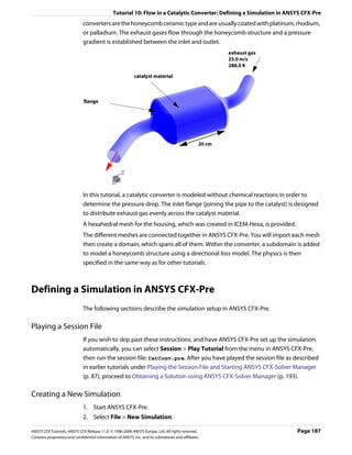
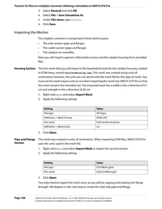
![Tutorial 10: Flow in a Catalytic Converter: Defining a Simulation in ANSYS CFX-Pre
Applying a Transform
The pipe and flange are located at the outlet end of the housing. The flange will be rotated
about an axis that points in the y-direction and is located at the center of the housing.
1. Right-click CatConvMesh.gtm and select Transform Mesh. The Mesh Transformation
Editor dialog box appears.
2. Apply the following settings
Tab Setting Value
Definition Apply Rotation > Rotation Option Rotation Axis
Apply Rotation > From 0, 0, 0.16
Apply Rotation > To 0, 1, 0.16*
Apply Rotation > Rotation Angle 180 [degree]
Multiple Copies (Selected)
Multiple Copies > # of Copies 1
*. This specifies an axis located at the center of the housing parallel to the y-axis.
3. Click OK.
Creating a Union Region
Three separate regions now exist, but since there is no relative motion between each region,
you only need to create a single domain. This can be done by simply using all three regions
in the domain Location list or, as in this case, by using the Region details view to create a
union of the three regions.
1. Create a new composite region named CatConverter.
2. Apply the following settings
Tab Setting Value
Basic Settings Dimension (Filter) 3D
Region List B1.P3, B1.P3 2, LIVE
3. Click OK.
Creating the Domain
For this simulation you will use an isothermal heat transfer model and assume turbulent
flow.
1. Click Domain and set the name to CatConv.
2. Apply the following settings
ANSYS CFX Tutorials. ANSYS CFX Release 11.0. © 1996-2006 ANSYS Europe, Ltd. All rights reserved. Page 189
Contains proprietary and confidential information of ANSYS, Inc. and its subsidiaries and affiliates.](https://image.slidesharecdn.com/ansys11tutorial-111218135319-phpapp01/85/Ansys-11-tutorial-201-320.jpg)
![Tutorial 10: Flow in a Catalytic Converter: Defining a Simulation in ANSYS CFX-Pre
Tab Setting Value
General Basic Settings > Location CatConverter
Options
Basic Settings > Fluid List Air Ideal Gas
Domain Models > Pressure > Reference Pressure 1 [atm]
Fluid Models Heat Transfer > Option Isothermal
Heat Transfer > Fluid Temperature 600 [K]
3. Click OK.
Creating a Subdomain to Model the Catalyst Structure
The catalyst-coated honeycomb structure will be modeled using a subdomain with a
directional source of resistance.
For quadratic resistances, the pressure drop is modeled using:
∂p
------ = – K Q U U i
- (Eqn. 1)
∂x i
where K Q is the quadratic resistance coefficient, U i is the local velocity in the i direction,
∂p
and ------ is the pressure drop gradient in the i direction.
-
∂x i
1. Select Insert > Subdomain from the main menu or click Subdomain
2. In the Insert Subdomain dialog box, type catalyst.
3. Apply the following settings
Tab Setting Value
Basic Settings Location LIVE*
Sources† Sources (Selected)
Sources > Momentum Source/Porous Loss (Selected)
Sources > Momentum Source/Porous Loss > (Selected)
Directional Loss
*. This is the entire housing section.
†. Used to set sources of momentum, resistance and mass for the subdomain (Other
sources are available for different problem physics).
4. Apply the following settings in the Directional Loss section
Setting Value
Streamwise Direction > X Component 0
Streamwise Direction > Y Component 0
Streamwise Direction > Z Component 1
Page 190 ANSYS CFX Tutorials. ANSYS CFX Release 11.0. © 1996-2006 ANSYS Europe, Ltd. All rights reserved.
Contains proprietary and confidential information of ANSYS, Inc. and its subsidiaries and affiliates.](https://image.slidesharecdn.com/ansys11tutorial-111218135319-phpapp01/85/Ansys-11-tutorial-202-320.jpg)
![Tutorial 10: Flow in a Catalytic Converter: Defining a Simulation in ANSYS CFX-Pre
Setting Value
Streamwise Loss > Option Linear and Quadratic
Coefs
Streamwise Loss > Quadratic Resistance Coefficient (Selected)
Streamwise Loss > Quadratic Resistance Coefficient > Quadratic 650 [kg m^-4]
Coefficient
5. Click OK.
Creating Boundary Conditions
Inlet Boundary 1. Create a new boundary condition named Inlet.
2. Apply the following settings
Tab Setting Value
Basic Settings Boundary Type Inlet
Location PipeEnd 2
Boundary Details Mass and Momentum > Normal Speed 25 [m s^-1]
3. Click OK.
Outlet 1. Create a new boundary condition named Outlet.
Boundary 2. Apply the following settings
Tab Setting Value
Basic Settings Boundary Type Outlet
Location PipeEnd
Boundary Details Mass and Momentum > Option Static Pressure
Mass and Momentum > Relative Pressure 0 [Pa]
3. Click OK.
The remaining surfaces are automatically grouped into the default no slip wall
boundary condition.
Creating the Domain Interfaces
Domain interfaces are used to define the connecting boundaries between meshes where
the faces do not match or when a frame change occurs. Meshes are ‘glued’ together using
the General Grid Interface (GGI) functionality of ANSYS CFX. Different types of GGI
connections can be made. In this case, you require a simple Fluid-Fluid Static connection (no
Frame Change). Other options allow you to change reference frame across the interface or
create a periodic boundary with dissimilar meshes on each periodic face.
Two Interfaces are required, one to connect the inlet flange to the catalyst housing and one
to connect the outlet flange to the catalyst housing.
ANSYS CFX Tutorials. ANSYS CFX Release 11.0. © 1996-2006 ANSYS Europe, Ltd. All rights reserved. Page 191
Contains proprietary and confidential information of ANSYS, Inc. and its subsidiaries and affiliates.](https://image.slidesharecdn.com/ansys11tutorial-111218135319-phpapp01/85/Ansys-11-tutorial-203-320.jpg)
![Tutorial 10: Flow in a Catalytic Converter: Defining a Simulation in ANSYS CFX-Pre
Inlet Pipe / 1. Create a new domain interface named InletSide.
Housing 2. Apply the following settings
Interface
Tab Setting Value
Basic Settings Interface Side 1 > Region List FlangeEnd 2
Interface Side 2 > Region List INLET
3. Click OK.
Outlet Pipe / 1. Create a new domain interface named OutletSide.
Housing 2. Apply the following settings
Interface
Tab Setting Value
Basic Settings Interface Side 1 > Region List FlangeEnd
Interface Side 2 > Region List OUTLET
3. Click OK.
Setting Initial Values
A sensible guess for the initial velocity is to set it to the expected velocity through the
catalyst housing. As the inlet velocity is 25 [m s^-1] and the cross sectional area of the inlet
and housing are known, you can apply conservation of mass to obtain an approximate
velocity of 2 [m s^-1] through the housing.
1. Click Global Initialization .
2. Apply the following settings
Tab Setting Value
Global Initial Conditions > Cartesian Velocity Automatic with Value
Settings Components > Option
Initial Conditions > Cartesian Velocity 0 [m s^-1]
Components > U
Initial Conditions > Cartesian Velocity 0 [m s^-1]
Components > V
Initial Conditions > Cartesian Velocity -2 [m s^-1]
Components > W
Initial Conditions > Turbulence Eddy (Selected)
Dissipation
3. Click OK.
Setting Solver Control
Assuming velocities of 25 [m s^-1] in the inlet and outlet pipes, and 2 [m s^-1] in the catalyst
housing, an approximate fluid residence time of 0.1 [s] can be calculated. A sensible
timestep of 0.04 [s] (1/4 to 1/2 of the fluid residence time) will be applied.
Page 192 ANSYS CFX Tutorials. ANSYS CFX Release 11.0. © 1996-2006 ANSYS Europe, Ltd. All rights reserved.
Contains proprietary and confidential information of ANSYS, Inc. and its subsidiaries and affiliates.](https://image.slidesharecdn.com/ansys11tutorial-111218135319-phpapp01/85/Ansys-11-tutorial-204-320.jpg)
![Tutorial 10: Flow in a Catalytic Converter: Obtaining a Solution using ANSYS CFX-Solver Manager
For the convergence criteria, an RMS value of at least 1e-05 is usually required for adequate
convergence, but the default value is sufficient for demonstration purposes.
1. Click Solver Control .
2. Apply the following settings
Tab Setting Value
Basic Settings Convergence Control > Fluid Timescale Physical Timescale
Control > Timescale Control
Convergence Control >Fluid Timescale 0.04 [s]
Control > Physical Timescale
3. Click OK.
Writing the Solver (.def) File
While writing the solver file, you will use the Summarize Interface Data option to display
information about the connection type used for each domain interface.
1. Click Write Solver File .
2. Apply the following settings
Setting Value
File name CatConv.def
Summarize Interface Data (Selected)
Quit CFX–Pre * (Selected)
*. If using ANSYS CFX-Pre in Standalone Mode.
3. Ensure Start Solver Manager is selected and click Save.
4. Once ANSYS CFX-Solver Manager launches, return to ANSYS CFX-Pre.
The Interface Summary dialog box is displayed. This displays information related to the
summary of interface connections.
5. Click OK.
6. If using Standalone Mode, quit ANSYS CFX-Pre, saving the simulation (.cfx) file at your
discretion.
Obtaining a Solution using ANSYS CFX-Solver Manager
When ANSYS CFX-Pre has shut down and the ANSYS CFX-Solver Manager has started, you
can obtain a solution to the CFD problem by following the instructions below:
1. Ensure Define Run is displayed.
2. Click Start Run.
ANSYS CFX-Solver runs and attempts to obtain a solution. This can take a long time
depending on your system. Eventually a dialog box is displayed.
ANSYS CFX Tutorials. ANSYS CFX Release 11.0. © 1996-2006 ANSYS Europe, Ltd. All rights reserved. Page 193
Contains proprietary and confidential information of ANSYS, Inc. and its subsidiaries and affiliates.](https://image.slidesharecdn.com/ansys11tutorial-111218135319-phpapp01/85/Ansys-11-tutorial-205-320.jpg)
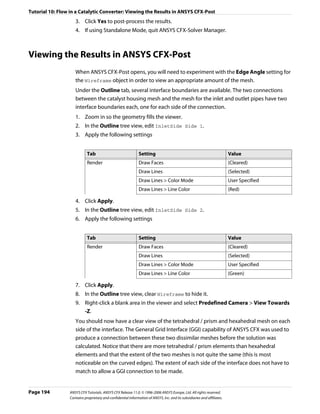
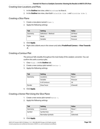
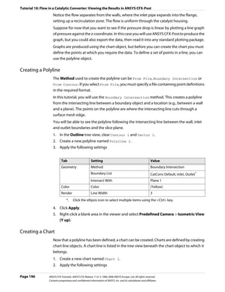
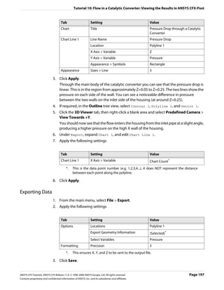
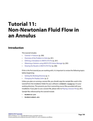
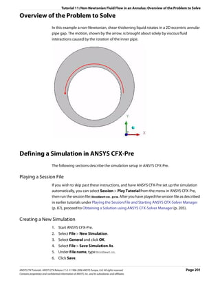
![Tutorial 11: Non-Newtonian Fluid Flow in an Annulus: Defining a Simulation in ANSYS CFX-Pre
Importing the Mesh
1. Right-click Mesh and select Import Mesh.
2. Apply the following settings
Setting Value
File name NonNewtonMesh.gtm
3. Click Open.
Creating an Expression for Shear Rate Dependent Viscosity
You can use an expression to define the dependency of fluid properties on other variables.
In this case, the fluid does not obey the simple linear Newtonian relationship between shear
stress and shear strain rate. The general relationship for the fluid you will model is given by:
n–1
µ = Kγ (Eqn. 1)
where γ is the shear strain rate and K and n are constants. For your fluid, n =1.5 and this
results in shear-thickening behavior of the fluid, i.e., the viscosity increases with increasing
shear strain rate. The shear strain rate is available as a ANSYS CFX-Pre System Variable
(sstrnr).
In order to describe this relationship using CEL, the dimensions must be consistent on both
sides of the equation. Clearly this means that K must have dimensions and requires units to
satisfy the equation. If the units of viscosity are kg m^-1 s^-1, and those of γ are s^-1, then
the expression is consistent if the units of K are kg m^-1 s^(-0.5).
1. Create the following expressions, remembering to click Apply after each is defined.
Name Definition
K 10.0 [kg m^-1 s^-0.5]
n 1.5
You should bound the viscosity to ensure that it remains physically meaningful. To do
so, you will create two additional parameters that will be used to guarantee the value of
the shear strain rate.
2. Create the following expressions for upper and lower bounds.
Name Definition
UpperS 100 [s^-1]
LowerS 1.0E-3 [s^-1]
ViscEqn K*(min(UpperS,max(sstrnr,LowerS))^(n-1))
3. Close the Expressions tab.
Page 202 ANSYS CFX Tutorials. ANSYS CFX Release 11.0. © 1996-2006 ANSYS Europe, Ltd. All rights reserved.
Contains proprietary and confidential information of ANSYS, Inc. and its subsidiaries and affiliates.](https://image.slidesharecdn.com/ansys11tutorial-111218135319-phpapp01/85/Ansys-11-tutorial-214-320.jpg)
![Tutorial 11: Non-Newtonian Fluid Flow in an Annulus: Defining a Simulation in ANSYS CFX-Pre
Creating a New Fluid
1. Create a new material named myfluid.
2. Apply the following settings
Tab Setting Value
Basic Settings Thermodynamic State (Selected)
Material Properties Equation of State > Molar Mass 1 [kg kmol^-1]*
Equation of State > Density 1.0E+4 [kg m^-3]
Specific Heat Capacity (Selected)
Specific Heat Capacity > Specific Heat Capacity 0 [J kg^-1 K^-1]†
Reference State (Selected)
Reference State > Option Specified Point
Reference State > Ref. Temperature 25 [C]
Reference State > Reference Pressure 1 [atm]
Transport Properties > Dynamic Viscosity (Selected)
Transport Properties > Dynamic Viscosity > ViscEqn
Dynamic Viscosity
*. This is not the correct Molar Mass value, but this material property will not be used
by the ANSYS CFX-Solver for this case. In other cases it will be used.
†. This is not the correct value for specific heat, but this property will not be used in
the ANSYS CFX-Solver.
3. Click OK.
Creating the Domain
1. Click Domain and set the name to NonNewton.
2. Apply the following settings to NonNewton
Tab Setting Value
General Basic Settings > Fluids List myfluid
Options Domain Models > Pressure > Reference Pressure 1 [atm]
Fluid Models Heat Transfer > Option Isothermal
Heat Transfer > Fluid Temperature 25 C
Turbulence > Option None (Laminar)
3. Click OK.
Creating the Boundary Conditions
Wall Boundary 1. Create a new boundary condition named rotwall.
2. Apply the following settings
ANSYS CFX Tutorials. ANSYS CFX Release 11.0. © 1996-2006 ANSYS Europe, Ltd. All rights reserved. Page 203
Contains proprietary and confidential information of ANSYS, Inc. and its subsidiaries and affiliates.](https://image.slidesharecdn.com/ansys11tutorial-111218135319-phpapp01/85/Ansys-11-tutorial-215-320.jpg)
![Tutorial 11: Non-Newtonian Fluid Flow in an Annulus: Defining a Simulation in ANSYS CFX-Pre
Tab Setting Value
Basic Settings Boundary Type Wall
Location rotwall
Boundary Details Wall Influence on Flow > Wall Velocity (Selected)
Wall Influence on Flow > Wall Velocity > Rotating Wall
Option
Wall Influence on Flow > Wall Velocity > 31.33 [rev min^-1]
Angular Velocity
3. Click OK.
Symmetry Plane 1. Create a new boundary condition named SymP1.
Boundary 2. Apply the following settings
Tab Setting Value
Basic Settings Boundary Type Symmetry
Location SymP1
3. Click OK.
4. Create a new boundary condition named SymP2.
5. Apply the following settings
Tab Setting Value
Basic Settings Boundary Type Symmetry
Location SymP2
6. Click OK.
The outer annulus surfaces will default to the no-slip stationary wall boundary
condition.
Setting Initial Values
A reasonable initial guess for the velocity field is a value of zero throughout the domain.
1. Click Global Initialization .
2. Apply the following settings
Tab Setting Value
Global Initial Conditions > Cartesian Velocity Components > Option Automatic with
Settings Value
Initial Conditions > Cartesian Velocity Components > U 0 [m s^-1]
Initial Conditions > Cartesian Velocity Components > V 0 [m s^-1]
Initial Conditions > Cartesian Velocity Components > W 0 [m s^-1]
3. Click OK.
Page 204 ANSYS CFX Tutorials. ANSYS CFX Release 11.0. © 1996-2006 ANSYS Europe, Ltd. All rights reserved.
Contains proprietary and confidential information of ANSYS, Inc. and its subsidiaries and affiliates.](https://image.slidesharecdn.com/ansys11tutorial-111218135319-phpapp01/85/Ansys-11-tutorial-216-320.jpg)
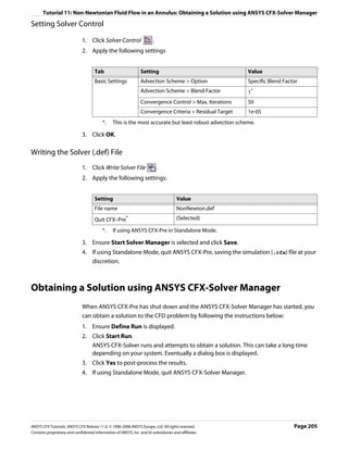
![Tutorial 11: Non-Newtonian Fluid Flow in an Annulus: Viewing the Results in ANSYS CFX-Post
Viewing the Results in ANSYS CFX-Post
In this tutorial you have used CEL to create an expression for the dynamic viscosity. If you
now perform calculations or color graphics objects using the Dynamic Viscosity variable, its
values will have been calculated from the expression you defined in ANSYS CFX-Pre.
These steps instruct the user on how to create a vector plot to show the velocity values in
the domain.
1. Right-click a blank area in the viewer and select Predefined Camera > View Towards
-Z from the shortcut menu.
2. Create a new plane named Plane 1.
3. Apply the following settings
Tab Setting Value
Geometry Definition > Method Point and Normal
Definition > Point 0, 0, 0.02
Definition > Normal 0, 0, 1
Plane Bounds > Type Circular
Plane Bounds > Radius 0.3 [m]
Plane Type Sample
Plane Type > R Samples 32
Plane Type > Theta Samples 24
Render Draw Faces (Cleared)
4. Click Apply.
5. Create a new vector plot named Vector 1.
6. Apply the following settings
Tab Setting Value
Geometry Definition > Locations Plane 1
Definition > Variable Velocity
Symbol Symbol Size 3
7. Click Apply.
8. Try creating some plots of your own, including one that shows the variation of dynamic
viscosity.
9. When you have finished, quit ANSYS CFX-Post.
Page 206 ANSYS CFX Tutorials. ANSYS CFX Release 11.0. © 1996-2006 ANSYS Europe, Ltd. All rights reserved.
Contains proprietary and confidential information of ANSYS, Inc. and its subsidiaries and affiliates.](https://image.slidesharecdn.com/ansys11tutorial-111218135319-phpapp01/85/Ansys-11-tutorial-218-320.jpg)
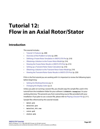
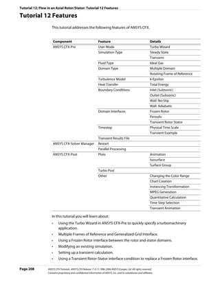
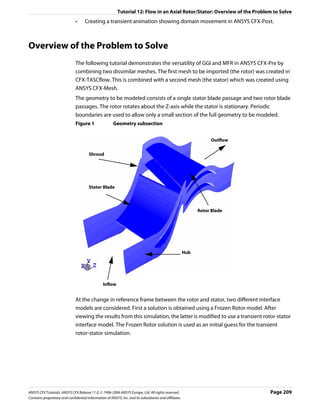

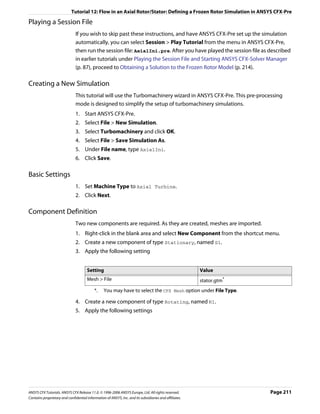
![Tutorial 12: Flow in an Axial Rotor/Stator: Defining a Frozen Rotor Simulation in ANSYS CFX-Pre
Setting Value
Component Type > Value 523.6 [radian s^-1]
Mesh File > File rotor.grd*
*. You may have to select the CFX-TASCflow option under File Type.
Note: The components must be ordered as above (stator then rotor) in order for the
interface to be created correctly. The order of the two components can be changed by right
clicking on S1 and selecting Move Component Up.
When a component is defined, Turbo Mode will automatically select a list of regions that
correspond to certain boundary condition types. This information should be reviewed
in the Region Information section to ensure that all is correct. This information will be
used to help set up boundary conditions and interfaces. The upper case turbo regions
that are selected (e.g., HUB) correspond to the region names in the CFX-TASCflow grd
file. CFX-TASCflow turbomachinery meshes use these names consistently.
6. Click Next.
Physics Definition
In this section, you will set properties of the fluid domain and some solver parameters.
1. Apply the following settings
Tab Setting Value
Physics Fluid Air Ideal Gas
Definition Simulation Type > Type Steady State
Model Data > Reference Pressure 0.25 [atm]
Model Data > Heat Transfer Total Energy
Model Data > Turbulence k-Epsilon
Boundary Templates > P-Total Inlet Mass Flow Outlet (Selected)
Boundary Templates > P-Total 0 [atm]
Boundary Templates > T-Total 340 [K]
Boundary Templates > Mass Flow Rate 0.06 [kg s^-1]
Interface > Default Type Frozen Rotor
Solver Parameters > Convergence Control Physical Timescale
Solver Parameters > Physical Timescale 0.002 [s]*
*. This time scale is approximately equal to 1 / ω , which is often appropriate for
rotating machinery applications.
2. Click Next.
Page 212 ANSYS CFX Tutorials. ANSYS CFX Release 11.0. © 1996-2006 ANSYS Europe, Ltd. All rights reserved.
Contains proprietary and confidential information of ANSYS, Inc. and its subsidiaries and affiliates.](https://image.slidesharecdn.com/ansys11tutorial-111218135319-phpapp01/85/Ansys-11-tutorial-224-320.jpg)
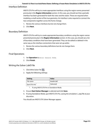
![Tutorial 12: Flow in an Axial Rotor/Stator: Setting up a Transient Rotor-Stator Calculation
Tab Setting Value
Physics Fluid Air Ideal Gas
Definition
Simulation Type > Type Transient
Simulation Type > Total Time 2.124e-4 [s]*
Simulation Type > Time Steps 2.124e-5 [s]†
Interface > Default Type Transient Rotor Stator
*. This gives 10 timesteps of 2.124e-5 s
†. This timestep will be used until the total time is reached
Note: A transient rotor-stator calculation often runs through more than one pitch. In these
cases, it may be useful to look at variable data averaged over the time interval required to
complete 1 pitch. You can then compare data for each pitch rotation to see if a “steady state”
has been achieved, or if the flow is still developing.
4. Click Next.
Interface Definition is displayed.
5. Click Next.
Boundary Definition is displayed.
6. Click Next.
Final Operations is displayed.
7. Ensure that Operation is set to Enter General Mode.
8. Click Finish.
Initial values are required, but will be supplied later using a results file.
Setting Output Control
1. Click Output Control .
2. Click the Trn Results tab.
3. Create a new transient result with the name Transient Results 1.
4. Apply the following settings to Transient Results 1
Setting Value
Option Selected Variables
Output Variables List * Pressure, Velocity, Velocity in Stn Frame
Output Frequency > Option Time Interval
Output Frequency > Time Interval 2.124e-5 [s]
*. Use the <Ctrl> key to select more than one variable.
5. Click OK.
Writing the Solver (.def) File
1. Click Write Solver File .
Page 218 ANSYS CFX Tutorials. ANSYS CFX Release 11.0. © 1996-2006 ANSYS Europe, Ltd. All rights reserved.
Contains proprietary and confidential information of ANSYS, Inc. and its subsidiaries and affiliates.](https://image.slidesharecdn.com/ansys11tutorial-111218135319-phpapp01/85/Ansys-11-tutorial-230-320.jpg)
![Tutorial 12: Flow in an Axial Rotor/Stator: Viewing the Transient Rotor-Stator Results in ANSYS CFX-Post
2. Under the Color panel select Variable and set it to Pressure with a user specified range
of -10000 [Pa] to -7000 [Pa].
Setting up Instancing Transformations
Next, you will use instancing transformations to view a larger section of the model. The
properties for each domain have already been entered during the initialization phase, so
only the number of instances needs to be set.
1. In the Turbo tree view, double-click the 3D View object.
2. In the Instancing section of the form, set # of Copies to 6 for R1.
3. Click Apply.
4. In the Instancing section of the form, set # of Copies to 6 for S1.
5. Click Apply.
6. Return to the Outline tab and ensure that the turbo surface is visible again.
Creating a Transient Animation
Start by loading the first timestep:
1. Click Timestep Selector .
2. Select time value 0.
3. Click Apply to load the timestep.
The rotor blades move to their starting position. This is exactly 1 pitch from the previous
position so the blades will not appear to move.
4. Clear Visibility for Wireframe.
5. Position the geometry as shown below, ready for the animation. During the animation
the rotor blades will move to the right. Make sure you have at least two rotor blades out
of view to the left side of the viewer. They will come into view during the animation.
6. In the toolbar at the top of the window click Animation .
7. In the Animation dialog box, click New to create KeyFrameNo1.
8. Highlight KeyframeNo1, then set # of Frames to 9.
9. Use the Timestep Selector to load the final timestep.
ANSYS CFX Tutorials. ANSYS CFX Release 11.0. © 1996-2006 ANSYS Europe, Ltd. All rights reserved. Page 221
Contains proprietary and confidential information of ANSYS, Inc. and its subsidiaries and affiliates.](https://image.slidesharecdn.com/ansys11tutorial-111218135319-phpapp01/85/Ansys-11-tutorial-233-320.jpg)
![Tutorial 13: Reacting Flow in a Mixing Tube: Defining a Simulation in ANSYS CFX-Pre
Tab Setting Value
Material Properties Thermodynamic Properties > Equation of State 19.52 [kg kmol^-1]*
> Molar Mass
Thermodynamic Properties > Equation of State 1080 [kg m^-3]
> Density
Thermodynamic Properties > Specific Heat (Selected)
Capacity
Thermodynamic Properties > Specific Heat 4190 [J kg^-1 K^-1]
Capacity > Specific Heat Capacity
Transport Properties > Dynamic Viscosity (Selected)
Transport Properties > Dynamic Viscosity > Value
Option
Transport Properties > Dynamic Viscosity > 0.001 [kg m^-1 s^-1]
Dynamic Viscosity
Transport Properties > Thermal Conductivity (Selected)
Transport Properties > Thermal Conductivity > 0.6 [W m^-1 K^-1]
Thermal Conductivity
*. The Molar Masses for the three materials created are only set for completeness
since they are not used when solving this problem.
3. Click OK.
Alkali 1. Create a new material named alkali.
properties 2. Apply the following settings
Tab Setting Value
Basic Settings Option Pure Substance
Thermodynamic State (Selected)
Thermodynamic State > Thermodynamic State Liquid
Material Properties Thermodynamic Properties > Equation of State 20.42 [kg kmol^-1]
> Molar Mass
Thermodynamic Properties > Equation of State 1130 [kg m^-3]
> Density
Thermodynamic Properties > Specific Heat (Selected)
Capacity
Thermodynamic Properties > Specific Heat 4190 [J kg^-1 K^-1]
Capacity > Specific Heat Capacity
Transport Properties > Dynamic Viscosity (Selected)
Transport Properties > Dynamic Viscosity > 0.001 [kg m^-1 s^-1]
Dynamic Viscosity
Transport Properties > Thermal Conductivity (Selected)
Transport Properties > Thermal Conductivity > 0.6 [W m^-1 K^-1]
Thermal Conductivity
3. Click OK.
ANSYS CFX Tutorials. ANSYS CFX Release 11.0. © 1996-2006 ANSYS Europe, Ltd. All rights reserved. Page 227
Contains proprietary and confidential information of ANSYS, Inc. and its subsidiaries and affiliates.](https://image.slidesharecdn.com/ansys11tutorial-111218135319-phpapp01/85/Ansys-11-tutorial-239-320.jpg)
![Tutorial 13: Reacting Flow in a Mixing Tube: Defining a Simulation in ANSYS CFX-Pre
Product of the 1. Create a new material named product.
reaction 2. Apply the following settings
properties
Tab Setting Value
Basic Settings Option Pure Substance
Thermodynamic State (Selected)
Thermodynamic State > Thermodynamic State Liquid
Material Properties Thermodynamic Properties > Equation of State 21.51 [kg kmol^-1]
> Molar Mass
Thermodynamic Properties > Equation of State 1190 [kg m^-3]
> Density
Thermodynamic Properties > Specific Heat (Selected)
Capacity
Thermodynamic Properties > Specific Heat 4190 [J kg^-1 K^-1]
Capacity > Specific Heat Capacity
Transport Properties > Dynamic Viscosity (Selected)
Transport Properties > Dynamic Viscosity > 0.001 [kg m^-1 s^-1]
Dynamic Viscosity
Transport Properties > Thermal Conductivity (Selected)
Transport Properties > Thermal Conductivity > 0.6 [W m^-1 K^-1]
Thermal Conductivity
3. Click OK.
Fluid properties 1. Create a new material named mixture.
2. Apply the following settings
Tab Setting Value
Basic Settings Option Variable Composition Mixture
Material Group User, Water Data
Materials List Water, acid, alkali, product
Thermodynamic State (Selected)
Thermodynamic State > Liquid
Thermodynamic State
3. Click OK.
Creating an Additional Variable to Model pH
You are going to use an additional variable to model the distribution of pH in the mixing
tube. You can create additional variables and use them in selected fluids in your domain.
1. Create a new additional variable named MixturePH.
2. Apply the following settings
Page 228 ANSYS CFX Tutorials. ANSYS CFX Release 11.0. © 1996-2006 ANSYS Europe, Ltd. All rights reserved.
Contains proprietary and confidential information of ANSYS, Inc. and its subsidiaries and affiliates.](https://image.slidesharecdn.com/ansys11tutorial-111218135319-phpapp01/85/Ansys-11-tutorial-240-320.jpg)
![Tutorial 13: Reacting Flow in a Mixing Tube: Defining a Simulation in ANSYS CFX-Pre
Tab Setting Value
Basic Settings Units [kg kg^-1]
3. Click OK.
This additional variable is now available for use when you create or modify a domain.
Defining the Reaction
Reactions and reaction kinetics can be modeled using CFX Expression Language (CEL),
together with appropriate settings for Component sources. This section shows you how to
develop an Eddy Break Up (EBU) type term using CEL to simulate the reaction between acid
and alkali.
Reaction Source The reaction and reaction rate are modeled using a basic Eddy Break Up formulation for the
Terms component and energy sources, so that, for example, the transport equation for mass
fraction of acid is
∂
d ---- ( ρm f acid ) + ∇•( ρU mf acid ) – ∇ • ( ρD A ∇m f acid )
-
∂t
(Eqn. 3)
ε mf alkali
= – 4ρ --min ⎛ mf acid, ---------------- ⎞
-
k ⎝ i ⎠
where mf is mass fraction, D A is the kinematic diffusivity (set above) and i is the
stoichiometric ratio. The right hand side represents the source term applied to the transport
equation for the mass fraction of acid. The left hand side consists of the transient, advection
and diffusion terms.
For acid-alkali reactions, the stoichiometric ratio is usually based on volume fractions. To
correctly model the reaction using an Eddy Break Up formulation based on mass fractions,
you must calculate the stoichiometric ratio based on mass fractions.
In this tutorial the reaction is modeled by introducing source terms for the acid, alkali and
product components. You can now also model this type of flow more easily using a reacting
mixture as your fluid. There is also a tutorial example using a reacting mixture. For details,
see Tutorial 18: Combustion and Radiation in a Can Combustor (p. 299).
Technical Note (Reference Only)
In ANSYS CFX, Release 11.0, a source is fully specified by an expression for its value S.
A source coefficient C is optional, but can be specified to provide convergence
enhancement or stability for strongly-varying sources. The value of C may affect the rate of
convergence but should not affect the converged results.
ANSYS CFX Tutorials. ANSYS CFX Release 11.0. © 1996-2006 ANSYS Europe, Ltd. All rights reserved. Page 229
Contains proprietary and confidential information of ANSYS, Inc. and its subsidiaries and affiliates.](https://image.slidesharecdn.com/ansys11tutorial-111218135319-phpapp01/85/Ansys-11-tutorial-241-320.jpg)
![Tutorial 13: Reacting Flow in a Mixing Tube: Defining a Simulation in ANSYS CFX-Pre
If no suitable value is available for C , the solution time scale or timestep can still be reduced
to help improve convergence of difficult source terms.
Important: C must never be positive.
An optimal value for C when solving an individual equation for a positive variable φ with a
source S whose strength decreases with increasing φ is
∂S
C = (Eqn. 4)
∂φ
Where this derivative cannot be computed easily,
S
C = --
- (Eqn. 5)
φ
may be sufficient to ensure convergence.
Another useful recipe for C is
ρ
C = – --
- (Eqn. 6)
τ
where τ is a local estimate for the source time scale. Provided that the source time scale is
not excessively short compared to flow or mixing time scales, this may be a useful approach
for controlling sources with positive feedback ( ∂S ⁄ ∂φ > 0 ) or sources that do not depend
directly on the solved variable φ .
Calculating pH The pH (or acidity) of the mixture is a function of the mass fraction of acid, alkali and product.
For the purposes of this calculation, acid is assumed to be dilute and fully dissociated into
+ -
its respective ions ( H and X ); alkali is assumed to be dilute and fully dissociated into its
+ -
respective ions ( Y and OH ); product is assumed to be a salt solution including further
+ -
H and OH ions in a stoichiometric ratio.
The concentrations of hydrogen and hydroxyl ions can be calculated from the mass
fractions of the components using the following expressions:
mf prod
[ H ] acid = αρ ⎛ mf acid + --------------- ⎞ = [ X ]
+ i–i
- (Eqn. 7)
⎝ 1+i ⎠
imf prod
[ OH ] alkali = βρ ⎛ mf alkali + ----------------- ⎞ = [ Y ]
- i+i
- (Eqn. 8)
⎝ 1+i ⎠
Page 230 ANSYS CFX Tutorials. ANSYS CFX Release 11.0. © 1996-2006 ANSYS Europe, Ltd. All rights reserved.
Contains proprietary and confidential information of ANSYS, Inc. and its subsidiaries and affiliates.](https://image.slidesharecdn.com/ansys11tutorial-111218135319-phpapp01/85/Ansys-11-tutorial-242-320.jpg)
![Tutorial 13: Reacting Flow in a Mixing Tube: Defining a Simulation in ANSYS CFX-Pre
- +
where α and β are the X ion and Y ion concentrations in the acid and alkali
-
respectively. For this problem, α is set to 1.0E-05 kmole X per kg of acid, and β = α ⁄ i .
Applying charge conservation and equilibrium conditions,
+ + - -
[ H ] + [ Y ] = [ X ] + [ OH ] (Eqn. 9)
+ -
[ H ] [ OH ] = K W (Eqn. 10)
gives the following quadratic equation for free hydrogen ion concentration:
+ + + -
[ H ] ( [ H ] + [ Y ] –[ X ] ) = K W (Eqn. 11)
+ 2 + - +
[H ] + ([Y ] – [X ])[H ] – K W = 0 (Eqn. 12)
i+i
pH = – log 10 [ H ] (Eqn. 13)
where K W is the equilibrium constant (1.0 x 10E-14 kmoles2 m-6).
+
The quadratic equation can be solved for [ H ] using the equation
2
+ – b + b – 4ac + -
[ H ] = ------------------------------------- where a = 1 , b = [ Y ] – [ X ] and c = – K W .
-
2a
Creating You can create the expressions required to model the reaction sources and pH by either
expressions to reading them in from a file or by defining them in the Expressions workspace. Note that the
model the
expressions used here do not refer to a particular fluid since there is only a single fluid. In a
reaction
multiphase simulation you must prefix variables with a fluid name, for example
Mixture.acid.mf instead of acid.mf.
In this tutorial the expressions can be imported from a file to avoid typing them.
Reading 1. Select File > Import CCL.
expressions 2. Ensure that Import Method is set to Append.
from a file
3. Select ReactorExpressions.ccl, which should be in your working directory.
4. Click Open.
Note that the expressions have been loaded.
Creating the Domain
1. Right click Simulation in the Outline tree view and ensure that Automatic Default
Domain is selected. A domain named Default Domain should now appear under the
Simulation branch.
2. Double click Default Domain and apply the following settings
ANSYS CFX Tutorials. ANSYS CFX Release 11.0. © 1996-2006 ANSYS Europe, Ltd. All rights reserved. Page 231
Contains proprietary and confidential information of ANSYS, Inc. and its subsidiaries and affiliates.](https://image.slidesharecdn.com/ansys11tutorial-111218135319-phpapp01/85/Ansys-11-tutorial-243-320.jpg)
![Tutorial 13: Reacting Flow in a Mixing Tube: Defining a Simulation in ANSYS CFX-Pre
Tab Setting Value
General Basic Settings > Domain Type Fluid Domain
Options
Basic Settings > Fluids List mixture
Domain Models > Pressure > Reference Pressure 1 [atm]
Fluid Models Heat Transfer > Option Thermal Energy
Component Details acid
Component Details > acid > Option Transport Equation
Component Details > acid > Kinematic Diffusivity (Selected)
Component Details > acid > Kinematic Diffusivity > 0.001 [m^2 s^-1]
Kinematic Diffusivity
3. Use the same Option and Kinematic Diffusivity settings for alkali and product as
you have just set for acid.
4. For Water, set Option to Constraint as follows
Tab Setting Value
Fluid Models Component Details Water
Component Details > Water > Option Constraint
One component must always use Constraint. This is the component used to balance
the mass fraction equation; the sum of the mass fractions of all components of a fluid
must equal unity.
5. Apply the following settings
Tab Setting Value
Fluid Models Additional Variable Details > MixturePH (Selected)
Additional Variable Details > MixturePH > Algebraic Equation
Option
Additional Variable Details > MixturePH > pH
Value
6. Click OK.
Creating a Subdomain to Model the Chemical Reactions
To provide the correct modeling for the chemical reaction you need to define sources for
the fluid components acid, alkali ,and product. To do this, you need to create a
subdomain where the relevant sources can be specified. In this case, sources need to be
provided within the entire domain of the mixing tube since the reaction occurs throughout
the domain.
1. Create a new subdomain named sources.
2. Apply the following settings
Page 232 ANSYS CFX Tutorials. ANSYS CFX Release 11.0. © 1996-2006 ANSYS Europe, Ltd. All rights reserved.
Contains proprietary and confidential information of ANSYS, Inc. and its subsidiaries and affiliates.](https://image.slidesharecdn.com/ansys11tutorial-111218135319-phpapp01/85/Ansys-11-tutorial-244-320.jpg)
![Tutorial 13: Reacting Flow in a Mixing Tube: Defining a Simulation in ANSYS CFX-Pre
Tab Setting Value
Sources Sources (Selected)
Sources > Equation Sources acid.mf
Sources > Equation Sources > acid.mf (Selected)
Sources > Equation Sources > acid.mf > Source AcidSource
Sources > Equation Sources > acid.mf > Source Coefficient (Selected)
Sources > Equation Sources > acid.mf > Source Coefficient > AcidSourceCoeff
Source Coefficient
Sources > Equation Sources alkali.mf
Sources > Equation Sources > alkali.mf (Selected)
Sources > Equation Sources > alkali.mf > Source AlkaliSource
Sources > Equation Sources > alkali.mf > Source Coefficient (Selected)
Sources > Equation Sources > alkali.mf > Source Coefficient > AlkaliSourceCoeff
Source Coefficient
Sources > Equation Sources Energy
Sources > Equation Sources > Energy (Selected)
Sources > Equation Sources > Energy > Source HeatSource
Sources > Equation Sources product.mf
Sources > Equation Sources > product.mf (Selected)
Sources > Equation Sources > product.mf > Source ProductSource
Sources > Equation Sources > product.mf > Source Coefficient (Selected)
Sources > Equation Sources > product.mf > Source Coefficient 0 [kg m^-3 s^-1]
> Source Coefficient
3. Click OK.
Creating the Boundary Conditions
Water Inlet 1. Create a new boundary condition named InWater.
Boundary 2. Apply the following settings
Tab Setting Value
Basic Settings Boundary Type Inlet
Location InWater
Boundary Details Mass and Momentum > Normal Speed 2 [m s^-1]
Heat Transfer > Option Static Temperature
Heat Transfer > Static Temperature 300 [K]
3. Leave mass fractions for all components set to zero. Since Water is the constraint fluid,
it will be automatically given a mass fraction of 1 on this inlet.
4. Click OK.
Acid Inlet 1. Create a new boundary condition named InAcid.
Boundary
ANSYS CFX Tutorials. ANSYS CFX Release 11.0. © 1996-2006 ANSYS Europe, Ltd. All rights reserved. Page 233
Contains proprietary and confidential information of ANSYS, Inc. and its subsidiaries and affiliates.](https://image.slidesharecdn.com/ansys11tutorial-111218135319-phpapp01/85/Ansys-11-tutorial-245-320.jpg)
![Tutorial 13: Reacting Flow in a Mixing Tube: Defining a Simulation in ANSYS CFX-Pre
2. Apply the following settings
Tab Setting Value
Basic Settings Boundary Type Inlet
Location InAcid
Boundary Details Mass and Momentum > Normal Speed 2 [m s^-1]
Heat Transfer > Option Static Temperature
Heat Transfer > Static Temperature 300 [K]
Component Details acid
Component Details > acid > Mass Fraction 1.0
Component Details alkali
Component Details > alkali > Mass Fraction 0
Component Details product
Component Details > product > Mass Fraction 0
3. Click OK.
Alkali Inlet The inlet area for the alkali is twice that of the acid and it also enters at a higher velocity. The
Boundary result is an acid-to-alkali volume inflow ratio of 1:2.667. Recall that a stoichiometric ratio of
2.7905 was specified based on mass fractions. When the density of the acid (1080 [kg m^3])
and alkali (1130 [kg m^3]) are considered, the acid-to-alkali mass flow ratio can be
calculated as 1:2.7905. You are therefore providing enough acid and alkali to produce a
neutral solution if they react together completely.
1. Create a new boundary condition named InAlkali.
2. Apply the following settings
Tab Setting Value
Basic Settings Boundary Type Inlet
Location InAlkali
Boundary Details Mass and Momentum > Normal Speed 2.667 [m s^-1]
Heat Transfer > Option Static Temperature
Heat Transfer > Static Temperature 300 [K]
Component Details > acid (Selected)
Component Details > acid > Mass Fraction 0
Component Details > alkali (Selected)
Component Details > alkali > Mass Fraction 1
Component Details > product (Selected)
Component Details > product > Mass Fraction 0
3. Click OK.
Outlet 1. Create a new boundary condition named out.
Boundary 2. Apply the following settings
Page 234 ANSYS CFX Tutorials. ANSYS CFX Release 11.0. © 1996-2006 ANSYS Europe, Ltd. All rights reserved.
Contains proprietary and confidential information of ANSYS, Inc. and its subsidiaries and affiliates.](https://image.slidesharecdn.com/ansys11tutorial-111218135319-phpapp01/85/Ansys-11-tutorial-246-320.jpg)
![Tutorial 13: Reacting Flow in a Mixing Tube: Defining a Simulation in ANSYS CFX-Pre
Tab Setting Value
Basic Settings Boundary Type Outlet
Location out
Boundary Details Mass and Momentum > Option Static Pressure
Mass and Momentum > Relative Pressure 0 [Pa]
3. Click OK.
Symmetry 1. Create a new boundary condition named sym1.
Boundary 2. Apply the following settings
Tab Setting Value
Basic Settings Boundary Type Symmetry
Location sym1
3. Click OK.
4. Create a new boundary condition named sym2.
5. Apply the following settings
Tab Setting Value
Basic Settings Boundary Type Symmetry
Location sym2
6. Click OK.
The default adiabatic wall boundary condition will automatically be applied to the
remaining unspecified boundary.
Setting Initial Values
The values for acid, alkali and product will be initialized to 0. Since Water is the
constrained component, it will make up the remaining mass fraction which, in this case, is 1.
1. Click Global Initialization .
2. Apply the following settings
ANSYS CFX Tutorials. ANSYS CFX Release 11.0. © 1996-2006 ANSYS Europe, Ltd. All rights reserved. Page 235
Contains proprietary and confidential information of ANSYS, Inc. and its subsidiaries and affiliates.](https://image.slidesharecdn.com/ansys11tutorial-111218135319-phpapp01/85/Ansys-11-tutorial-247-320.jpg)
![Tutorial 13: Reacting Flow in a Mixing Tube: Defining a Simulation in ANSYS CFX-Pre
Tab Setting Value
Global Initial Conditions > Cartesian Velocity Components > Automatic with Value
Settings Option
Initial Conditions > Cartesian Velocity Components > U 2 [m s^-1]
Initial Conditions > Cartesian Velocity Components > V 0 [m s^-1]
Initial Conditions > Cartesian Velocity Components > W 0 [m s^-1]
Initial Conditions > Turbulence Eddy Dissipation (Selected)
Initial Conditions > Turbulence Eddy Dissipation > Automatic
Option
Initial Conditions > Component Details acid
Initial Conditions > Component Details > acid > Option Automatic with Value
Initial Conditions > Component Details > acid > Mass 0
Fraction
Initial Conditions > Component Details alkali
Initial Conditions > Component Details > alkali > Option Automatic with Value
Initial Conditions > Component Details > alkali > Mass 0
Fraction
Initial Conditions > Component Details product
Initial Conditions > Component Details > product > Automatic with Value
Option
Initial Conditions > Component Details > product > Mass 0
Fraction
3. Click OK.
Setting Solver Control
1. Click Solver Control .
2. Apply the following settings
Tab Setting Value
Basic Settings Advection Scheme > Option Specific Blend Factor
Advection Scheme > Blend Factor 0.75
Convergence Control > Max. Iterations 50
Convergence Control > Fluid Timescale Physical Timescale
Control > Timescale Control
Convergence Control > Fluid Timescale 0.01 [s]*
Control > Physical Timescale
*. The length of mixing tube is 0.06 [m] and inlet velocity is 2 [m s^-1]. An estimate of
the dynamic time scale is 0.03 [s]. An appropriate timestep would be 1/4 to 1/2 of
this value.
Page 236 ANSYS CFX Tutorials. ANSYS CFX Release 11.0. © 1996-2006 ANSYS Europe, Ltd. All rights reserved.
Contains proprietary and confidential information of ANSYS, Inc. and its subsidiaries and affiliates.](https://image.slidesharecdn.com/ansys11tutorial-111218135319-phpapp01/85/Ansys-11-tutorial-248-320.jpg)

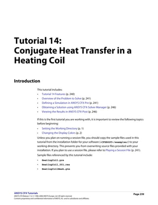
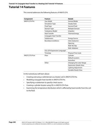

![Tutorial 14: Conjugate Heat Transfer in a Heating Coil: Defining a Simulation in ANSYS CFX-Pre
6. Click Save.
Importing the Mesh
1. Right-click Mesh and select Import Mesh.
2. Apply the following settings
Setting Value
File name HeatingCoilMesh.gtm
3. Click Open.
4. Right-click a blank area in the viewer and select Predefined Camera > Isometric View
(Z up) from the shortcut menu.
Creating the Domains
This simulation requires both a fluid and a solid domain. First, you will create a fluid domain
for the annular region of the heat exchanger.
Creating a Fluid The fluid domain will include the region of fluid flow but exclude the solid copper heater.
Domain
1. Click Domain and set the name to FluidZone.
2. Apply the following settings to FluidZone
Tab Setting Value
General Basic Settings > Location B1.P3*
Options
Basic Settings > Fluids List Water
Domain Models > Pressure > Reference Pressure 1 [atm]
Fluid Models Heat Transfer > Option Thermal Energy
Initialization Domain Initialization (Selected)
Domain Initialization > Initial Conditions (Selected)
Domain Initialization > Initial Conditions > Turbulence (Selected)
Eddy Dissipation
*. This region name may be different depending on how the mesh was created. You
should pick the region that forms the exterior surface of the volume surrounding
the coil.
3. Click OK.
Creating a Solid Since you know that the copper heating element will be much hotter than the fluid, you can
Domain initialize the temperature to a reasonable value. The initialization option that is set when
creating a domain applies only to that domain.
1. Create a new domain named SolidZone.
2. Apply the following settings
Page 242 ANSYS CFX Tutorials. ANSYS CFX Release 11.0. © 1996-2006 ANSYS Europe, Ltd. All rights reserved.
Contains proprietary and confidential information of ANSYS, Inc. and its subsidiaries and affiliates.](https://image.slidesharecdn.com/ansys11tutorial-111218135319-phpapp01/85/Ansys-11-tutorial-254-320.jpg)
![Tutorial 14: Conjugate Heat Transfer in a Heating Coil: Defining a Simulation in ANSYS CFX-Pre
Tab Setting Value
General Basic Settings > Location B2.P3
Options
Basic Settings > Domain Type Solid Domain
Basic Settings > Solids List Copper
Solid Models Heat Transfer > Option Thermal Energy
Initialization Domain Initialization (Selected)
Domain Initialization > Initial Conditions (Selected)
Domain Initialization > Initial Conditions > Automatic with
Temperature > Option Value
Domain Initialization > Initial Conditions > 550 [K]
Temperature > Temperature
3. Click OK.
Creating a Subdomain to Specify a Thermal Energy Source
To allow a thermal energy source to be specified for the copper heating element, you need
to create a subdomain.
1. Create a new subdomain named Heater in the domain SolidZone.
2. Apply the following settings
Tab Setting Value
Basic Settings Basic Settings > Location B2.P3*
Sources Sources (Selected)
Sources > Equation Sources > Energy (Selected)
Sources > Equation Sources > Energy > Source 1.0E+07 [W m^-3]
*. This is the same location as for the domain SolidZone, because you want the source
term to apply to the entire solid domain.
3. Click OK.
Creating the Boundary Conditions
Inlet Boundary You will now create an inlet boundary condition for the cooling fluid (Water).
1. Create a new boundary condition named inflow in the domain FluidZone.
2. Apply the following settings
Tab Setting Value
Basic Settings Boundary Type Inlet
Location inflow
Boundary Details Mass and Momentum > Normal Speed 0.4 [m s^-1]
Heat Transfer > Static Temperature 300 [K]
3. Click OK.
ANSYS CFX Tutorials. ANSYS CFX Release 11.0. © 1996-2006 ANSYS Europe, Ltd. All rights reserved. Page 243
Contains proprietary and confidential information of ANSYS, Inc. and its subsidiaries and affiliates.](https://image.slidesharecdn.com/ansys11tutorial-111218135319-phpapp01/85/Ansys-11-tutorial-255-320.jpg)
![Tutorial 14: Conjugate Heat Transfer in a Heating Coil: Defining a Simulation in ANSYS CFX-Pre
Opening The opening boundary condition type is used in this case because at some stage during the
boundary solution, the coiled heating element will cause some recirculation at the exit. At an opening
boundary you need to set the temperature of fluid that enters through the boundary. In this
case it is useful to base this temperature on the fluid temperature at the outlet, since you
expect the fluid to be flowing mostly out through this opening.
1. Create a new expression named OutletTemperature.
2. Set Definition to areaAve(T)@REGION:outflow
3. Click Apply.
4. Create a new boundary condition named outflow in the domain FluidZone.
5. Apply the following settings:
Tab Setting Value
Basic Settings Boundary Type Opening
Location outflow
Boundary Details Mass and Momentum > Option Opening Pres. and Dirn
Mass and Momentum > Relative Pressure 0 [Pa]
Heat Transfer > Option Static Temperature
Heat Transfer > Static Temperature OutletTemperature
6. Click OK.
The default adiabatic wall boundary condition will automatically be applied to the
remaining unspecified external boundaries of the fluid domain. The default Fluid-Solid
Interface boundary condition (flux conserved) will be applied to the surfaces between
the solid domain and the fluid domain.
Creating the Domain Interface
If you have the Generate Default Domain Interfaces option turned on (from Edit >
Options > CFX-Pre), then you will see that an interface called
Default Fluid Solid Interface already exists, and is listed in the Outline tree view. If
this is the case, you can optionally skip the following instructions for creating a domain
interface (since the domain interface set here will have the same settings as, and will
automatically replace, the default domain interface).
If you have the Generate Default Domain Interfaces option turned off, then there is no
domain interface defined at this point. In this case, create a domain interface using either
one of the following methods (the result is the same):
Creating a 1. Right click Simulation in the Outline tree view and ensure that Automatic Default
Default Domain Interfaces is selected. An interface named Default Fluid Solid Interface should
Interface
now appear under the Simulation branch.
Creating a 1. Double click Default Fluid Solid Interface and apply the following settings:
Domain
Interface
Manually
Page 244 ANSYS CFX Tutorials. ANSYS CFX Release 11.0. © 1996-2006 ANSYS Europe, Ltd. All rights reserved.
Contains proprietary and confidential information of ANSYS, Inc. and its subsidiaries and affiliates.](https://image.slidesharecdn.com/ansys11tutorial-111218135319-phpapp01/85/Ansys-11-tutorial-256-320.jpg)
![Tutorial 14: Conjugate Heat Transfer in a Heating Coil: Defining a Simulation in ANSYS CFX-Pre
Tab Setting Value
Basic Settings Interface Type Fluid Solid
Interface Side 1 > Domain (Filter) FluidZone
Interface Side 1 > Region List F10.B1.P3, F5.B1.P3,
F6.B1.P3, F7.B1.P3, F8.B1.P3,
F9.B1.P3
Interface Side 2 > Domain (Filter) SolidZone
Interface Side 2 > Region List F10.B2.P3, F5.B2.P3,
F6.B2.P3, F7.B2.P3, F8.B2.P3,
F9.B2.P3
Interface Models > Option General Connection
Interface Models > Frame Change/Mixing None
Model > Option
Interface Models > Pitch Change > Option None
Mesh Connection Method > Option Automatic
2. Click OK.
Setting Solver Control
1. Click Solver Control .
2. Apply the following settings:
Tab Setting Value
Basic Settings Convergence Control > Fluid Timescale Physical Timescale
Control > Timescale Control
Convergence Control >Fluid Timescale 2 [s]
Control > Physical Timescale
For the Convergence Criteria, an RMS value of at least 1e-05 is usually required for
adequate convergence, but the default value is sufficient for demonstration purposes.
3. Click OK.
Writing the Solver (.def) File
1. Click Write Solver File .
2. Apply the following settings:
Setting Value
File name HeatingCoil.def
Quit CFX–Pre * (Selected)
*. If using ANSYS CFX-Pre in Standalone Mode.
3. Ensure Start Solver Manager is selected and click Save.
ANSYS CFX Tutorials. ANSYS CFX Release 11.0. © 1996-2006 ANSYS Europe, Ltd. All rights reserved. Page 245
Contains proprietary and confidential information of ANSYS, Inc. and its subsidiaries and affiliates.](https://image.slidesharecdn.com/ansys11tutorial-111218135319-phpapp01/85/Ansys-11-tutorial-257-320.jpg)
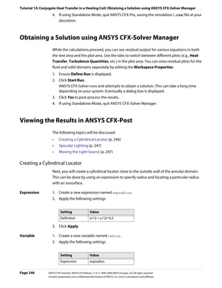
![Tutorial 14: Conjugate Heat Transfer in a Heating Coil: Exporting the Results to ANSYS
3. Click Apply.
Isosurface of the 1. Create a new isosurface named Isosurface 1.
variable 2. Apply the following settings
Tab Setting Value
Geometry Definition > Variable radius
Definition > Value 0.8 [m]*
Color Mode Variable
Variable Temperature
Range User Specified
Min 300 [K]
Max 302 [K]
Render Draw Faces (Selected)
*. The maximum radius is 1 m, so a cylinder locator at a radius of 0.8 m is suitable.
3. Click Apply.
Specular Lighting
Specular lighting is on by default. Specular lighting allows glaring bright spots on the
surface of an object, depending on the orientation of the surface and the position of the
light.
1. Apply the following settings to Isosurface 1
Tab Setting Value
Render Draw Faces > Specular (Cleared)
2. Click Apply.
Moving the Light Source
To move the light source, click within the 3-D Viewer, then press and hold <Shift> while
pressing the arrow keys left, right, up or down.
Tip: If using the Standalone version, you can move the light source by positioning the
mouse pointer in the viewer, holding down the <Ctrl> key, and dragging using the right
mouse button.
Exporting the Results to ANSYS
This optional step involves generating an ANSYS .cdb data file from the results generated
in ANSYS CFX-Solver. The .cdb file could then be used with the ANSYS Multi-field solver to
measure the combined effects of thermal and mechanical stresses on the solid heating coil.
There are two possible ways to export data to ANSYS:
ANSYS CFX Tutorials. ANSYS CFX Release 11.0. © 1996-2006 ANSYS Europe, Ltd. All rights reserved. Page 247
Contains proprietary and confidential information of ANSYS, Inc. and its subsidiaries and affiliates.](https://image.slidesharecdn.com/ansys11tutorial-111218135319-phpapp01/85/Ansys-11-tutorial-259-320.jpg)
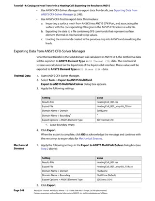


![Tutorial 15: Multiphase Flow in Mixing Vessel: Defining a Simulation in ANSYS CFX-Pre
Tab Setting Value
General Basic Settings > Location Main
Options
Basic Settings > Fluids List Air at 25 C, Water
Domain Models > Pressure > Reference Pressure 1 [atm]
Domain Models > Buoyancy > Option Buoyant
Domain Models > Buoyancy > Gravity X Dirn. -9.81 [m s^-2]
Domain Models > Buoyancy > Gravity Y Dirn. 0 [m s^-2]
Domain Models > Buoyancy > Gravity Z Dirn. 0 [m s^-2]
Domain Models > Buoyancy > Buoy. Ref. Density* 997 [kg m^-3]
Domain Models > Domain Motion > Option Rotating
Domain Models > Domain Motion > Angular Velocity 84 [rev min-1]†
Domain Models > Domain Motion > Axis Definition > Global X
Rotation Axis
Fluid Multiphase Options > Homogeneous Model (Cleared)
Models Multiphase Options > Allow Musig Fluids (Cleared)
Multiphase Options > Free Surface Model > Option None
Heat Transfer > Homogeneous Model (Cleared)
Heat Transfer > Option Isothermal
Heat Transfer > Fluid Temperature 25 [C]
Turbulence > Homogeneous Model (Cleared)
Turbulence > Option Fluid Dependent
Fluid Fluid Details Air at 25 C
Details
Fluid Details > Air at 25 C > Morphology > Option Dispersed Fluid
Fluid Details > Air at 25 C > Morphology > Mean Diameter 3 [mm]
Fluid Fluid Pairs Air at 25 C | Water
Pairs Fluid Pairs > Air at 25 C | Water > Surface Tension Coefficient (Selected)
Fluid Pairs > Air at 25 C | Water > Surface Tension Coefficient 0.073 [N m^-1]‡
> Surf. Tension Coeff.
Fluid Pairs > Air at 25 C | Water > Momentum Transfer > Drag Grace
Force > Option
Fluid Pairs > Air at 25 C | Water > Momentum Transfer > Drag (Selected)
Force > Volume Fraction Correction Exponent
Fluid Pairs > Air at 25 C | Water > Momentum Transfer > Drag 4
Force > Volume Fraction Correction Exponent > Value
Fluid Pairs > Air at 25 C | Water > Momentum Transfer > Lopez de
Non-drag forces > Turbulent Dispersion Force > Option Bertodano
Fluid Pairs > Air at 25 C | Water > Momentum Transfer > 0.1
Non-drag forces > Turbulent Dispersion Force > Dispersion
Coeff.
Fluid Pairs > Air at 25 C | Water > Turbulence Transfer > Sato Enhanced
Option Eddy Viscosity
Page 256 ANSYS CFX Tutorials. ANSYS CFX Release 11.0. © 1996-2006 ANSYS Europe, Ltd. All rights reserved.
Contains proprietary and confidential information of ANSYS, Inc. and its subsidiaries and affiliates.](https://image.slidesharecdn.com/ansys11tutorial-111218135319-phpapp01/85/Ansys-11-tutorial-268-320.jpg)
![Tutorial 15: Multiphase Flow in Mixing Vessel: Defining a Simulation in ANSYS CFX-Pre
Tab Setting Value
Fluid Values Boundary Conditions Air at 25 C
Boundary Conditions > Air at 25 C > Velocity 5 [m s^-1]
> Normal Speed
Boundary Conditions > Air at 25 C > Volume 1
Fraction > Volume Fraction
Boundary Conditions Water
Boundary Conditions > Water > Velocity > 5 [m s^-1]
Normal Speed
Boundary Conditions > Water > Volume 0
Fraction > Volume Fraction
3. Click OK.
Degassing 1. Create a new boundary condition in the domain tank named LiquidSurface.
Outlet 2. Apply the following settings
Boundary
Tab Setting Value
Basic Settings Boundary Type Outlet
Location WALL_LIQUID_SURFACE
Boundary Details Mass and Momentum > Option Degassing Condition
3. Click OK.
Thin Surface for In ANSYS CFX-Pre, thin surfaces can be created by specifying wall boundary conditions on
the Baffle both sides of internal 2D regions. Both sides of the baffle regions will be specified as walls in
this case.
1. Create a new boundary condition in the domain tank named Baffle.
2. Apply the following settings
Tab Setting Value
Basic Settings Boundary Type Wall
Location WALL_BAFFLES*
Boundary Details Wall Influence On Flow > Option Fluid Dependent
Fluid Values Boundary Conditions Air at 25 C
Boundary Conditions > Air at 25 C > Wall Free Slip
Influence on Flow > Option
Boundary Conditions Water
Boundary Conditions > Water > Wall No Slip†
Influence on Flow > Option
*. The WALL_BAFFLES region includes the surfaces on both sides of the baffle (you can
confirm this by examining WALL_BAFFLES in the region selector). Therefore, you do
not need to use the Create Thin Surface Partner option.
†. The Free Slip condition can be used for the gas phase since the contact area with
the walls is near zero for low gas phase volume fractions.
3. Click OK.
Page 258 ANSYS CFX Tutorials. ANSYS CFX Release 11.0. © 1996-2006 ANSYS Europe, Ltd. All rights reserved.
Contains proprietary and confidential information of ANSYS, Inc. and its subsidiaries and affiliates.](https://image.slidesharecdn.com/ansys11tutorial-111218135319-phpapp01/85/Ansys-11-tutorial-270-320.jpg)
![Tutorial 15: Multiphase Flow in Mixing Vessel: Defining a Simulation in ANSYS CFX-Pre
Wall Boundary The next stage involves setting up a boundary condition for the shaft, which exists in the
Condition for tank (stationary domain). These regions are connected to the shaft in the impeller domain.
the Shaft
Since the tank domain is not rotating, you need to specify a moving wall to account for the
rotation of the shaft.
Part of the shaft is located directly above the air inlet, so the volume fraction of air in this
location will be high and the assumption of zero contact area for the gas phase is not
physically correct. In this case, a no slip boundary condition is more appropriate than a free
slip condition for the air phase. When the volume fraction of air in contact with a wall is low,
a free slip condition is more appropriate for the air phase.
In cases where it is important to correctly model the dispersed phase slip properties at walls
for all volume fractions, you can declare both fluids as no slip, but set up an expression for
the dispersed phase wall area fraction. The expression should result in an area fraction of
zero for dispersed phase volume fractions from 0 to 0.3, for example, and then linearly
increase to an area fraction of 1 as the volume fraction increases to 1.
1. Create a new boundary condition in the domain tank named TankShaft.
2. Apply the following settings
Tab Setting Value
Basic Settings Boundary Type Wall
Location WALL_SHAFT,
WALL_SHAFT_CENTER
Boundary Details Wall Influence On Flow > Option Fluid Dependent
Fluid Values Boundary Conditions Air at 25 C
Boundary Conditions > Air at 25 C > Wall No Slip
Influence on Flow > Option
Boundary Conditions > Air at 25 C > Wall (Selected)
Influence on Flow > Wall Velocity
Boundary Conditions > Air at 25 C > Wall Rotating Wall
Influence on Flow > Wall Velocity > Option
Boundary Conditions > Air at 25 C > Wall 84 [rev min-1]*
Influence on Flow > Wall Velocity > Angular
Velocity
Boundary Conditions > Air at 25 C > Wall Global X
Influence on Flow > Wall Velocity > Axis
Definition > Rotation Axis
*. Note the unit.
3. Select Water and set the same values as for Air at 25 C.
4. Click OK.
Required 1. Create a new boundary condition in the domain impeller named Blade.
Boundary 2. Apply the following settings
Conditions in
the Impeller
Domain
ANSYS CFX Tutorials. ANSYS CFX Release 11.0. © 1996-2006 ANSYS Europe, Ltd. All rights reserved. Page 259
Contains proprietary and confidential information of ANSYS, Inc. and its subsidiaries and affiliates.](https://image.slidesharecdn.com/ansys11tutorial-111218135319-phpapp01/85/Ansys-11-tutorial-271-320.jpg)

![Tutorial 15: Multiphase Flow in Mixing Vessel: Defining a Simulation in ANSYS CFX-Pre
Setting Initial Values
The initialization for volume fraction is 0 for air and automatic for water. Therefore, the initial
volume fraction for water will be set to 1 so that the sum of the two fluid volume fractions is
1.
It is important to understand how the velocity is initialized in this tutorial. Here, both fluids
use Automatic for the Cartesian Velocity Components. When the Automatic option is
used, the initial velocity field will be based on the velocity values set at inlets, openings, and
outlets. In this tutorial, the only boundary that has a set velocity value is the inlet, which
specifies a velocity of 5 [m s^-1] for both phases. Without setting the Velocity Scale
parameter, the resulting initial guess would be a uniform velocity of 5 [m s^-1] in the
X-direction throughout the domains for both phases. This is clearly not suitable since the
water phase is enclosed by the tank. When the boundary velocity conditions are not
representative of the expected domain velocities, the Velocity Scale parameter should be
used to set a representative domain velocity. In this case the velocity scale for water is set to
zero, causing the initial velocity for the water to be zero. The velocity scale is not set for air,
resulting in an initial velocity of 5 [m s^-1] in the X-direction for the air. This should not be a
problem since the initial volume fraction of the air is zero everywhere.
1. Click Global Initialization .
2. Apply the following settings
Tab Setting Value
Fluid Settings Fluid Specific Initialization Air at 25 C
Fluid Specific Initialization > Air at 25 C > Initial Automatic with Value
Conditions > Volume Fraction > Option
Fluid Specific Initialization > Air at 25 C > Initial 0
Conditions > Volume Fraction > Volume Fraction
Fluid Specific Initialization Water
Fluid Specific Initialization > Water > Initial (Selected)
Conditions > Cartesian Velocity Components >
Velocity Scale
Fluid Specific Initialization > Water > Initial 0 [m s^-1]
Conditions > Cartesian Velocity Components >
Velocity Scale > Value
Fluid Specific Initialization > Water > Initial (Selected)
Conditions > Turbulence Eddy Dissipation
3. Click OK.
Setting Solver Control
Generally, two different time scales exist for multiphase mixers. The first is a small time scale
based on the rotational speed of the impeller, typically taken as 1 / ω , resulting in a time
scale of 0.11 s for this case. The second time scale is usually larger and based on the
recirculation time of the continuous phase in the mixer.
ANSYS CFX Tutorials. ANSYS CFX Release 11.0. © 1996-2006 ANSYS Europe, Ltd. All rights reserved. Page 263
Contains proprietary and confidential information of ANSYS, Inc. and its subsidiaries and affiliates.](https://image.slidesharecdn.com/ansys11tutorial-111218135319-phpapp01/85/Ansys-11-tutorial-275-320.jpg)
![Tutorial 15: Multiphase Flow in Mixing Vessel: Defining a Simulation in ANSYS CFX-Pre
Using a timestep based on the rotational speed of the impeller will be more robust, but
convergence will be slow since it takes time for the flow field in the mixer to develop. Using
a larger timestep reduces the number of iterations required for the mixer flow field to
develop, but reduces robustness. You will need to experiment to find an optimum timestep.
Note: You may find it useful to monitor the value of an expression during the solver run so
that you can view the volume fraction of air in the tank (the gas hold up). The gas hold up is
often used to judge convergence in these types of simulations by converging until a
steady-state value is achieved. You could create the following expressions:
TankAirHoldUp = volumeAve(Air at 25 C.vf)@tank
ImpellerAirHoldUp = volumeAve(Air at 25 C.vf)@impeller
TotalAirHoldUp = (volume()@tank * TankAirHoldUp + volume()@impeller *
ImpellerAirHoldUp) / (volume()@tank + volume()@impeller)
and then monitor the value of TotalAirHoldUp.
1. Click Solver Control .
2. Apply the following settings
Tab Setting Value
Basic Settings Convergence Control > Fluid Timescale Physical Timescale
Control > Timescale Control
Convergence Control > Fluid Timescale 2 [s]*
Control > Physical Timescale
*. This is an aggressive timestep for this case.
3. Click OK.
Setting Output Control
In the next step, you will choose to write additional data to the results file which allows force
and torque calculations to be performed in post-processing.
1. Click Output Control .
2. Apply the following settings
Tab Setting Value
Results Output Boundary Flows (Selected)
Output Boundary Flows > Boundary Flows All
3. Click OK.
Writing the Solver (.def) File
Since this tutorial uses domain interfaces and you choose to summarize the interface data,
an information window is displayed that informs you of the connection type used for each
domain interface.
1. Click Write Solver File .
2. Apply the following settings:
Page 264 ANSYS CFX Tutorials. ANSYS CFX Release 11.0. © 1996-2006 ANSYS Europe, Ltd. All rights reserved.
Contains proprietary and confidential information of ANSYS, Inc. and its subsidiaries and affiliates.](https://image.slidesharecdn.com/ansys11tutorial-111218135319-phpapp01/85/Ansys-11-tutorial-276-320.jpg)
![Tutorial 15: Multiphase Flow in Mixing Vessel: Viewing the Results in ANSYS CFX-Post
Visualizing the Mixing Process
Creating a plane 1. Create a new plane named Plane 1.
2. Apply the following settings
Tab Setting Value
Geometry Definition > Method Three Points
Definition > Point 1 1, 0, 0
Definition > Point 2 0, 1, -0.9
Definition > Point 3 0, 0, 0
Color Mode Variable
Variable Air at 25 C.Volume Fraction
Range User Specified
Min 0
Max 0.04
3. Click Apply.
4. Observe the plane, then apply the following settings:
Tab Setting Value
Color Variable Air at 25 C.Shear Strain Rate
Range User Specified
Min 0 [s^-1]
Max 15 [s^-1]
5. Click Apply.
Areas of high shear strain rate or shear stress are typically also areas where the highest
mixing occurs.
6. Observe the plane, then apply the following settings:
Tab Setting Value
Color Variable Pressure
Range Local
7. Click Apply.
Note that the hydrostatic contribution to pressure is excluded due to the use of an
appropriate buoyancy reference density. If you plot the variable called Absolute
Pressure, you will see the true pressure including the hydrostatic contribution.
Creating a 1. Create a new vector named Vector 1.
vector 2. Apply the following settings
Page 266 ANSYS CFX Tutorials. ANSYS CFX Release 11.0. © 1996-2006 ANSYS Europe, Ltd. All rights reserved.
Contains proprietary and confidential information of ANSYS, Inc. and its subsidiaries and affiliates.](https://image.slidesharecdn.com/ansys11tutorial-111218135319-phpapp01/85/Ansys-11-tutorial-278-320.jpg)
![Tutorial 15: Multiphase Flow in Mixing Vessel: Viewing the Results in ANSYS CFX-Post
Tab Setting Value
Geometry Definition > Locations Plane 1
Variable Water.Velocity in Stn Frame*
Symbol Symbol Size 0.2
Normalize Symbols (Selected)
*. Using this variable, instead of Water.Velocity, results in the velocity vectors
appearing to be continuous at the interface between the rotating and stationary
domains. Velocity variables that do not include a frame specification always use the
local reference frame.
3. Observe the vector plot, then change the variable to Air at 25 C.Velocity in Stn
Frame. Observe this as well, then clear the visibility of Vector 1.
4. Modify the tank Default object.
5. Apply the following settings:
Tab Setting Value
Color Mode Variable
Variable Water.Wall Shear
Range Local
The legend for this plot shows the range of wall shear values.
The global maximum wall shear is much higher than the maximum value on the default
walls. The global maximum values occur on the TankShaft boundary directly above the
inlet. Although these values are very high, the shear force exerted on this boundary will
be small since the contact area fraction of water here is very small.
Calculating 1. Select Tools > Function Calculator from the main menu or click Show Function
Power and
Calculator from the main toolbar.
Torque
Required by the 2. Apply the following settings:
Impeller
Tab Setting Value
Function Function torque
Calculator Location Blade
Axis Global X
Fluid All Fluids
3. Click Calculate to find the torque required to rotate Blade about the X-axis.
4. Repeat the calculation setting Location to Blade Other Side.
The sum of these two results is the torque required by the single impeller blade,
approximately 70 [N m]. This must be multiplied by the number of blades in the full
geometry to obtain the total torque required by the impeller; the result is a value of
approximately 282 [N m]. You could also include the results from the locations HubShaft
and TankShaft; however in this case their contributions are negligible.
ANSYS CFX Tutorials. ANSYS CFX Release 11.0. © 1996-2006 ANSYS Europe, Ltd. All rights reserved. Page 267
Contains proprietary and confidential information of ANSYS, Inc. and its subsidiaries and affiliates.](https://image.slidesharecdn.com/ansys11tutorial-111218135319-phpapp01/85/Ansys-11-tutorial-279-320.jpg)
![Tutorial 15: Multiphase Flow in Mixing Vessel: Viewing the Results in ANSYS CFX-Post
The power requirement is simply the required torque multiplied by the rotational speed
(8.8 rad/s): Power = 282*8.8 = 2482 [W].
Remember that this value is the power requirement for the work done on the fluid only, it
does not account for any mechanical losses, efficiencies etc. Also note that the accuracy of
these results is significantly affected by the coarseness of the mesh. You should not use a
mesh of this length scale to obtain accurate quantitative results.
Page 268 ANSYS CFX Tutorials. ANSYS CFX Release 11.0. © 1996-2006 ANSYS Europe, Ltd. All rights reserved.
Contains proprietary and confidential information of ANSYS, Inc. and its subsidiaries and affiliates.](https://image.slidesharecdn.com/ansys11tutorial-111218135319-phpapp01/85/Ansys-11-tutorial-280-320.jpg)

![Tutorial 16: Gas-Liquid Flow in an Airlift Reactor: Defining a Simulation in ANSYS CFX-Pre
Setting Value
File name BubbleColumnMesh.gtm
3. Click Open.
Creating the Domain
1. Right click Simulation in the Outline tree view and ensure that Automatic Default
Domain is selected. A domain named Default Domain should now appear under the
Simulation branch.
2. Double click Default Domain and apply the following settings:
Tab Setting Value
General Basic Settings > Location B1.P3, B2.P3
Options
Basic Settings > Fluids List Air at 25 C, Water
Domain Models > Pressure > Reference Pressure 1 [atm]
Domain Models > Buoyancy > Option Buoyant
Domain Models > Buoyancy > Gravity X Dirn. 0 [m s^-2]
Domain Models > Buoyancy > Gravity Y Dirn. -9.81 [m s^-2]
Domain Models > Buoyancy > Gravity Z Dirn. 0 [m s^-2]
Domain Models > Buoyancy > Buoy. Ref. Density* 997 [kg m^-3]
Fluid Multiphase Options > Homogeneous Model (Cleared)
Models
Multiphase Options > Allow Musig Fluids (Cleared)
Free Surface Model > Option None
Heat Transfer > Option Isothermal
Heat Transfer > Fluid Temperature 25 C
Turbulence > Option Fluid Dependent
Fluid Fluid Details Air at 25 C
Details Fluid Details > Air at 25 C > Morphology > Option Dispersed Fluid
Fluid Details > Air at 25 C > Morphology > Mean Diameter 6 [mm]
Page 272 ANSYS CFX Tutorials. ANSYS CFX Release 11.0. © 1996-2006 ANSYS Europe, Ltd. All rights reserved.
Contains proprietary and confidential information of ANSYS, Inc. and its subsidiaries and affiliates.](https://image.slidesharecdn.com/ansys11tutorial-111218135319-phpapp01/85/Ansys-11-tutorial-284-320.jpg)
![Tutorial 16: Gas-Liquid Flow in an Airlift Reactor: Defining a Simulation in ANSYS CFX-Pre
Tab Setting Value
Fluid Fluid Pairs > Air at 25 C | Water > Surface Tension Coefficient (Selected)
Pairs Fluid Pairs > Air at 25 C | Water > Surface Tension Coefficient 0.072 [N m^-1]†
> Surf. Tension Coeff.
Fluid Pairs > Air at 25 C | Water > Momentum Transfer > Drag Grace
Force > Option
Fluid Pairs > Air at 25 C | Water > Momentum Transfer > Drag (Selected)
Force > Volume Fraction Correction Exponent
Fluid Pairs > Air at 25 C | Water > Momentum Transfer > Drag 2
Force > Volume Fraction Correction Exponent > Value
Fluid Pairs > Air at 25 C | Water > Momentum Transfer > Lopez de
Non-drag Forces > Turbulent Dispersion Force > Option Bertodano
Fluid Pairs > Air at 25 C | Water > Momentum Transfer > 0.3
Non-drag Forces > Turbulent Dispersion Force > Dispersion
Coeff.
Fluid Pairs > Air at 25 C | Water > Turbulence Transfer > Sato Enhanced
Option Eddy Viscosity
*. For dilute dispersed multiphase flow, always set the buoyancy reference density to
that for continuous fluid.
†. This must be set to allow the Grace drag model to be used.
3. Click OK.
Creating the Boundary Conditions
For this simulation of the airlift reactor, the boundary conditions required are:
• An inlet for air on the sparger.
• A degassing outlet for air at the liquid surface.
• A thin surface wall for the draft tube.
• An exterior wall for the outer wall, base and sparger tube.
• Symmetry planes for the cross sections.
Inlet Boundary There are an infinite number of inlet velocity/volume fraction combinations that will
produce the same mass inflow of air. The combination chosen gives an air inlet velocity
close to the terminal rise velocity. Since the water inlet velocity is zero, you can adjust its
volume fraction until the required mass flow rate of air is obtained for a given air inlet
velocity.
1. Create a new boundary condition named Sparger.
2. Apply the following settings
Tab Setting Value
Basic Settings Boundary Type Inlet
Location Sparger
Boundary Details Mass And Momentum > Option Fluid Dependent
ANSYS CFX Tutorials. ANSYS CFX Release 11.0. © 1996-2006 ANSYS Europe, Ltd. All rights reserved. Page 273
Contains proprietary and confidential information of ANSYS, Inc. and its subsidiaries and affiliates.](https://image.slidesharecdn.com/ansys11tutorial-111218135319-phpapp01/85/Ansys-11-tutorial-285-320.jpg)
![Tutorial 16: Gas-Liquid Flow in an Airlift Reactor: Defining a Simulation in ANSYS CFX-Pre
Tab Setting Value
Fluid Values Boundary Conditions Air at 25 C
Boundary Conditions > Air at 25 C > Velocity 0.3 [m s^-1]
> Normal Speed
Boundary Conditions > Air at 25 C > Volume 0.25
Fraction > Volume Fraction
Boundary Conditions Water
Boundary Conditions > Water > Velocity > 0 [m s^-1]
Normal Speed
Boundary Conditions > Water > Volume 0.75
Fraction > Volume Fraction
3. Click OK.
Outlet The top of the reactor will be a degassing boundary, which is classified as an outlet
Boundary boundary.
1. Create a new boundary condition named Top.
2. Apply the following settings
Tab Setting Value
Basic Settings Boundary Type Outlet
Location Top
Boundary Details Mass and Momentum > Option Degassing Condition
3. Click OK.
Thin Surface Thin surfaces are created by specifying a wall boundary condition on both sides of an
Draft Tube internal region. If only one side has a boundary condition then the ANSYS CFX-Solver will
Boundary
fail. To assist with this, you can select only one side of a thin surface and then enable the
Create Thin Surface Partner toggle. ANSYS CFX-Pre will then try to automatically create
another boundary condition for the other side.
1. Create a new boundary condition named DraftTube.
2. Apply the following settings
Tab Setting Value
Basic Settings Boundary Type Wall
Location Draft Tube
Thin Surfaces > Create Thin Surface Partner (Selected)
Boundary Details Wall Influence On Flow > Option Fluid Dependent
Fluid Values Boundary Conditions Air at 25 C
Boundary Conditions > Air at 25 C > Wall Free Slip
Influence On Flow > Option
Boundary Conditions Water
Boundary Conditions > Water > Wall No Slip
Influence On Flow > Option
Page 274 ANSYS CFX Tutorials. ANSYS CFX Release 11.0. © 1996-2006 ANSYS Europe, Ltd. All rights reserved.
Contains proprietary and confidential information of ANSYS, Inc. and its subsidiaries and affiliates.](https://image.slidesharecdn.com/ansys11tutorial-111218135319-phpapp01/85/Ansys-11-tutorial-286-320.jpg)

![Tutorial 16: Gas-Liquid Flow in an Airlift Reactor: Defining a Simulation in ANSYS CFX-Pre
1. Click Global Initialization .
Since a single pressure field exists for a multiphase calculation you do not set pressure
values on a per fluid basis.
2. Apply the following settings
Tab Setting Value
Fluid Settings Fluid Specific Initialization Air at 25 C
Fluid Specific Initialization > Air at 25 C (Selected)
Fluid Specific Initialization > Air at 25 C > Initial Automatic with Value
Conditions > Cartesian Velocity Components >
Option
Fluid Specific Initialization > Air at 25 C > Initial 0 [m s^-1]
Conditions > Cartesian Velocity Components > U
Fluid Specific Initialization > Air at 25 C > Initial 0.3 [m s^-1]
Conditions > Cartesian Velocity Components > V
Fluid Specific Initialization > Air at 25 C > Initial 0 [m s^-1]
Conditions > Cartesian Velocity Components > W
Fluid Specific Initialization Water*
Fluid Specific Initialization > Water (Selected)
Fluid Specific Initialization > Water > Initial Automatic with Value
Conditions > Cartesian Velocity Components >
Option
Fluid Specific Initialization > Water > Initial 0 [m s^-1]
Conditions > Cartesian Velocity Components > U
Fluid Specific Initialization > Water > Initial 0 [m s^-1]
Conditions > Cartesian Velocity Components > V
Fluid Specific Initialization > Water > Initial 0 [m s^-1]
Conditions > Cartesian Velocity Components > W
Fluid Specific Initialization > Water > Initial Automatic
Conditions > Turbulence Kinetic Energy > Option
Fluid Specific Initialization > Water > Initial (Selected)
Conditions > Turbulence Eddy Dissipation
Fluid Specific Initialization > Water > Initial Automatic
Conditions > Turbulence Eddy Dissipation >
Option
Fluid Specific Initialization > Water > Initial Automatic with Value
Conditions > Volume Fraction > Option
Fluid Specific Initialization > Water > Initial 1†
Conditions > Volume Fraction > Volume Fraction
*. Since there is no water entering or leaving the domain, a stationary initial guess is
recommended.
†. The volume fractions must sum to unity over all fluids. Since a value has been set for
water, the volume fraction of air will be calculated as the remaining difference, in
this case, 0.
3. Click OK.
Page 276 ANSYS CFX Tutorials. ANSYS CFX Release 11.0. © 1996-2006 ANSYS Europe, Ltd. All rights reserved.
Contains proprietary and confidential information of ANSYS, Inc. and its subsidiaries and affiliates.](https://image.slidesharecdn.com/ansys11tutorial-111218135319-phpapp01/85/Ansys-11-tutorial-288-320.jpg)
![Tutorial 16: Gas-Liquid Flow in an Airlift Reactor: Obtaining a Solution using ANSYS CFX-Solver Manager
Setting Solver Control
If you are using a maximum edge length of 0.005 m or less to produce a finer mesh, use a
Target Residual of 1.0E-05 to obtain a more accurate solution.
1. Click Solver Control .
2. Apply the following settings
Tab Setting Value
Basic Settings Convergence Control > Fluid Timescale Physical Timescale
Control > Timescale Control
Convergence Control > Fluid Timescale 1 [s]
Control > Physical Timescale
3. Click OK.
Writing the Solver (.def) File
1. Click Write Solver File .
2. Apply the following settings:
Setting Value
File name BubbleColumn.def
Quit CFX–Pre* (Selected)
*. If using ANSYS CFX-Pre in Standalone Mode.
3. Ensure Start Solver Manager is selected and click Save.
4. If using Standalone Mode, quit ANSYS CFX-Pre, saving the simulation (.cfx) file at your
discretion.
Obtaining a Solution using ANSYS CFX-Solver Manager
The ANSYS CFX-Solver Manager will be launched after ANSYS CFX-Pre has closed down. You
will be able to obtain a solution to the CFD problem by following the instructions below.
Note: If a fine mesh is used for a formal quantitative analysis of the flow in the reactor, the
solution time will be significantly longer than for the coarse mesh. You can run the
simulation in parallel to reduce the solution time. For details, see Obtaining a Solution in
Parallel (p. 116).
1. Ensure Define Run is displayed.
2. Click Start Run.
ANSYS CFX-Solver runs and attempts to obtain a solution. This can take a long time
depending on your system. Eventually a dialog box is displayed stating that the
simulation has completed.
ANSYS CFX Tutorials. ANSYS CFX Release 11.0. © 1996-2006 ANSYS Europe, Ltd. All rights reserved. Page 277
Contains proprietary and confidential information of ANSYS, Inc. and its subsidiaries and affiliates.](https://image.slidesharecdn.com/ansys11tutorial-111218135319-phpapp01/85/Ansys-11-tutorial-289-320.jpg)


![Tutorial 17: Air Conditioning Simulation: Defining a Simulation in ANSYS CFX-Pre
*. This is the name of the subroutine within the Fortran file. Always use lower case
letters for the calling name, even if the subroutine name in the Fortran file is in
upper case.
†. This is the name passed to the cfx5mkext command by the -name option. If the
-name option is not specified, a default is used. The default is the Fortran file name
without the .F extension.
‡. Set this to your working directory.
4. Click OK.
5. Create a new user function named Thermostat Function by selecting Insert >
Expressions, Functions and Variables > User Function from the main menu.
6. Apply the following settings
Tab Setting Value
Basic Settings Option User Function
Argument Units [K], [K], [K], []*
Result Units []†
*. These are the units for the four input arguments: TSensor, TSet, TTol, and aitern.
†. The result will be a dimensionless integer flag of values 1 or 0.
7. Click OK.
The function you have just prepared is called during the evaluation of the expression for
ACOn (that you imported earlier). The expression is:
Thermostat Function(TSensor,TSet,TTol,aitern)
It evaluates to 1 or 0, depending on whether the air conditioner should be on (1) or off
(0).
Setting the Simulation Type
1. Click Simulation Type .
2. Apply the following settings
Tab Setting Value
Basic Settings Simulation Type > Option Transient
Simulation Type > Time Duration > Total Time tTotal
Simulation Type > Time Steps > Timesteps tStep
Simulation Type > Initial Time > Time 0 [s]
3. Click OK.
Creating the Domain
1. Right click Simulation in the Outline tree view and ensure that Automatic Default
Domain is selected. A domain named Default Domain should now appear under the
Simulation branch.
2. Double click Default Domain and apply the following settings:
ANSYS CFX Tutorials. ANSYS CFX Release 11.0. © 1996-2006 ANSYS Europe, Ltd. All rights reserved. Page 289
Contains proprietary and confidential information of ANSYS, Inc. and its subsidiaries and affiliates.](https://image.slidesharecdn.com/ansys11tutorial-111218135319-phpapp01/85/Ansys-11-tutorial-301-320.jpg)
![Tutorial 17: Air Conditioning Simulation: Defining a Simulation in ANSYS CFX-Pre
Tab Setting Value
General Basic Settings > Location B1.P3
Options
Fluids List Air Ideal Gas
Domain Models > Pressure > Reference Pressure 1 [atm]
Domain Models > Buoyancy > Option Buoyant
Domain Models > Buoyancy > Gravity X Dirn. 0 [m s^-2]
Domain Models > Buoyancy > Gravity Y Dirn. 0 [m s^-2]
Domain Models > Buoyancy > Gravity Z Dirn. -g
Domain Models > Buoyancy > Buoy. Ref. Density 1.2 [kg m^-3]
Fluid Models Heat Transfer > Option Thermal Energy
Thermal Radiation Model > Option Monte Carlo
3. Click OK.
Setting Boundary Conditions
In this section you will define the locations and values of the boundary conditions.
Inlet Boundary 1. Create a new boundary condition named Inlet.
2. Apply the following settings
Tab Setting Value
Basic Settings Boundary Type Inlet
Location Inlet
Boundary Details Mass and Momentum > Option Mass Flow Rate
Mass and Momentum > Mass Flow Rate MassFlow
Flow Direction > Option Cartesian Components
Flow Direction > X Component XCompInlet
Flow Direction > Y Component 0
Flow Direction > Z Component ZCompInlet
Heat Transfer > Static Temperature TIn
Plot Options Boundary Vector (Selected)
3. Click OK.
Note: Ignore the physics errors that appear. They will be fixed by setting up the rest of the
simulation. The error you see is due to a reference to Thermometer which has not been set
up yet. This will be done as part of the output control.
Outlet 1. Create a new boundary condition named VentOut.
Boundary 2. Apply the following settings
Page 290 ANSYS CFX Tutorials. ANSYS CFX Release 11.0. © 1996-2006 ANSYS Europe, Ltd. All rights reserved.
Contains proprietary and confidential information of ANSYS, Inc. and its subsidiaries and affiliates.](https://image.slidesharecdn.com/ansys11tutorial-111218135319-phpapp01/85/Ansys-11-tutorial-302-320.jpg)
![Tutorial 17: Air Conditioning Simulation: Defining a Simulation in ANSYS CFX-Pre
Tab Setting Value
Basic Settings Boundary Type Outlet
Location VentOut
Boundary Details Mass and Momentum > Relative Pressure 0 [Pa]
3. Click OK.
Window To model incoming radiation at the window boundaries, a directional radiation source will
Boundary be created. The windows will also contribute heat to the room via a fixed temperature of
26 [C].
1. Create a new boundary condition named Windows.
2. Apply the following settings
Tab Setting Value
Basic Boundary Type Wall
Settings Location Window1, Window2
Boundary Heat Transfer > Option Temperature
Details Heat Transfer > Fixed Temperature 26 [C]
3. Apply the following settings
Tab Setting Value
Sources Boundary Source (Selected)
Boundary Source > Sources (Selected)
4. Create a new radiation source item by clicking Add New Item and accepting the
default name.
5. Apply the following settings to Radiation Source 1
Setting Value
Option Directional Radiation Flux
Radiation Flux 600 [W m^-2]
Direction > Option Cartesian Components
Direction > X Component 0.33
Direction > Y Component 0.33
Direction > Z Component -0.33
6. Apply the following setting
Tab Setting Value
Plot Boundary Vector (Selected)
Options
ANSYS CFX Tutorials. ANSYS CFX Release 11.0. © 1996-2006 ANSYS Europe, Ltd. All rights reserved. Page 291
Contains proprietary and confidential information of ANSYS, Inc. and its subsidiaries and affiliates.](https://image.slidesharecdn.com/ansys11tutorial-111218135319-phpapp01/85/Ansys-11-tutorial-303-320.jpg)
![Tutorial 17: Air Conditioning Simulation: Defining a Simulation in ANSYS CFX-Pre
7. Click OK.
The directional source of radiation is displayed.
Default Wall The default boundary condition for any undefined surface in ANSYS CFX-Pre is a no-slip,
Boundary smooth, adiabatic wall. For radiation purposes, the default wall is assumed to be a perfectly
absorbing and emitting surface (emissivity = 1), and this will be preserved when setting up
the boundary condition.
In this tutorial, a fixed temperature of 26 °C will be assumed to exist at the wall during the
simulation. A more detailed analysis would model heat transfer through the walls, but as
this tutorial is designed only for demonstration purposes, a fixed temperature wall is
sufficient.
1. Modify the boundary condition named Default Domain Default.
2. Apply the following settings
Tab Setting Value
Boundary Heat Transfer > Option Temperature
Details Heat Transfer > Fixed Temperature 26 [C]
3. Click OK.
This setting will include the Door region, which will be modeled as a wall (closed door) for
simplicity. Since the region is part of the entire default boundary, it will not appear in the
wireframe when the results file is opened in ANSYS CFX-Post (but can still be viewed in the
Regions list).
Setting Initial Values
1. Click Global Initialization .
2. Apply the following settings
Page 292 ANSYS CFX Tutorials. ANSYS CFX Release 11.0. © 1996-2006 ANSYS Europe, Ltd. All rights reserved.
Contains proprietary and confidential information of ANSYS, Inc. and its subsidiaries and affiliates.](https://image.slidesharecdn.com/ansys11tutorial-111218135319-phpapp01/85/Ansys-11-tutorial-304-320.jpg)
![Tutorial 17: Air Conditioning Simulation: Defining a Simulation in ANSYS CFX-Pre
Tab Setting Value
Global Settings Initial Conditions > Velocity Type Cartesian
Initial Conditions > Cartesian Velocity Automatic with Value
Components > Option
Initial Conditions > Cartesian Velocity 0 [m s^-1]
Components > U
Initial Conditions > Cartesian Velocity 0 [m s^-1]
Components > V
Initial Conditions > Cartesian Velocity 0 [m s^-1]
Components > W
Initial Conditions > Static Pressure > Relative 0 [Pa]
Pressure
Initial Conditions > Temperature > Temperature 22 [C]
Initial Conditions > Turbulence Kinetic Energy > (Selected)
Fractional Intensity
Initial Conditions > Turbulence Eddy Dissipation (Selected)
Initial Conditions > Turbulence Eddy Dissipation (Selected)
> Eddy Length Scale
Initial Conditions > Turbulence Eddy Dissipation 0.25 [m]
> Eddy Length Scale > Eddy Len. Scale
Initial Conditions > Radiation Intensity > (Selected)
Blackbody Temperature
Initial Conditions > Radiation Intensity > 22 [C]
Blackbody Temperature > Blackbody Temp.
3. Click OK.
Setting Solver Control
1. Click Solver Control .
2. Apply the following settings
Tab Setting Value
Basic Settings Transient Scheme > Option Second Order Backward
Euler
Convergence Control > Max. Coeff. Loops 3
3. Click OK.
Setting Output Control
Transient results files will be set up to record transient values of a chosen set of variables.
Monitor points will be created to show the on/off status of the air conditioner, the
temperature at the inlet, the temperature at the outlet, and the temperature at a prescribed
thermometer location.
ANSYS CFX Tutorials. ANSYS CFX Release 11.0. © 1996-2006 ANSYS Europe, Ltd. All rights reserved. Page 293
Contains proprietary and confidential information of ANSYS, Inc. and its subsidiaries and affiliates.](https://image.slidesharecdn.com/ansys11tutorial-111218135319-phpapp01/85/Ansys-11-tutorial-305-320.jpg)
![Tutorial 17: Air Conditioning Simulation: Viewing the Results in ANSYS CFX-Post
Creating Graphics Objects
Plane locators will be placed vertically through the vents and horizontally above the floor.
Plane Locators 1. Load the res file (HVAC_001.res) if you did not elect to load the results directly from the
ANSYS CFX-Solver Manager.
2. Right-click a blank area in the viewer, select Predefined Camera > Isometric View (Z
up).
3. Create a ZX-Plane named Plane 1 with Y=1.5 [m]. Color it by Temperature using a
user specified range from 19 [C] to 23 [C], and clear Lighting.
4. Create an XY Plane named Plane 2 with Z=0.35 [m]. Color it using the same settings
as for the first plane, and clear Lighting.
Isosurface 1. Click Timestep Selector .
Locator The Timestep Selector appears.
2. Double-click the value (12s) in the Timestep Selector.
The Timestep is set to 12s so that the cold plume is visible.
3. Create an isosurface named Cold Plume which is a surface of Temperature=19 [C].
Use conservative values for Temperature.
4. Color the isosurface by Temperature and use the same range as for the planes.
Although the color of the isosurface will not show variation (by definition), it will be
consistent with the other graphic objects.
5. On the Render tab for the isosurface, set Transparency to 0.5, and clear Lighting.
6. Click Apply.
Note: The isosurface will not be visible in some timesteps, but you will be able to see it when
playing the animation (a step carried out later).
Adjusting the The legend title should not name the locator of any particular object since all objects are
Legend colored by the same variable and use the same range.
1. In the tree view, double-click Default Legend View 1.
2. In the Definition tab, change Title Mode to Variable.
This will remove the locator name from the legend.
3. Click the Appearance tab, then:
a. Change Precision to 2, Fixed.
b. Change Text Height to 0.03.
4. Click Apply.
A label will be used to show the simulation time and the temperature of the thermometer
which controls the thermostat. This will be especially useful for the animation which is
created later in this tutorial.
Page 296 ANSYS CFX Tutorials. ANSYS CFX Release 11.0. © 1996-2006 ANSYS Europe, Ltd. All rights reserved.
Contains proprietary and confidential information of ANSYS, Inc. and its subsidiaries and affiliates.](https://image.slidesharecdn.com/ansys11tutorial-111218135319-phpapp01/85/Ansys-11-tutorial-308-320.jpg)
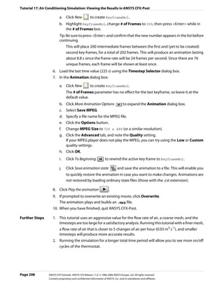

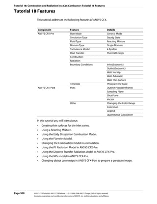

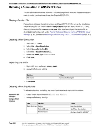
![Tutorial 18: Combustion and Radiation in a Can Combustor: Defining a Simulation in ANSYS CFX-Pre
Tab Setting Value
Mixture Mixture Properties (Selected)
Properties Mixture Properties > Radiation Properties > (Selected)†
Refractive Index
Mixture Properties > Radiation Properties > (Selected)
Absorption Coefficient
Mixture Properties > Radiation Properties > (Selected)
Scattering Coefficient
*. The Methane Air WD1 NO PDF reaction specifies complete combustion of the fuel
into its products in a single-step reaction. The formation of NO is also modeled and
occurs in an additional reaction step.
Click to display the Reactions List dialog box, then click Import Library Data
and select the appropriate reaction to import.
†. Setting the radiation properties explicitly will significantly shorten the solution time
since the ANSYS CFX-Solver will not have to calculate radiation mixture properties.
3. Click OK.
Creating the Domain
1. Right click Simulation in the Outline tree view and ensure that Automatic Default
Domain is selected. A domain named Default Domain should now appear under the
Simulation branch.
2. Double click Default Domain and apply the following settings
Tab Setting Value
General Basic Settings > Locations B152, B153, B154,
Options B155, B156
Basic Settings > Fluids List Methane Air Mixture
Domain Models > Pressure > Reference Pressure 1 [atm]*
Fluid Models Heat Transfer > Option Thermal Energy
Reaction or Combustion > Option Eddy Dissipation
Reaction or Combustion > Eddy Dissipation Model (Selected)
Coefficient B
Reaction or Combustion > Eddy Dissipation Model 0.5†
Coefficient B > EDM Coeff. B
Thermal Radiation Model > Option P1
Component Details > N2 (Selected)
Component Details > N2 > Option Constraint
*. It is important to set a realistic reference pressure in this tutorial because the
components of Methane Air Mixture are ideal gases.
†. This includes a simple model for partial premixing effects by turning on the Product
Limiter. When it is selected, non-zero initial values are required for the products. The
products limiter is not recommended for multi-step eddy dissipation reactions, and
so is set for this single step reaction only.
3. Click OK.
ANSYS CFX Tutorials. ANSYS CFX Release 11.0. © 1996-2006 ANSYS Europe, Ltd. All rights reserved. Page 303
Contains proprietary and confidential information of ANSYS, Inc. and its subsidiaries and affiliates.](https://image.slidesharecdn.com/ansys11tutorial-111218135319-phpapp01/85/Ansys-11-tutorial-315-320.jpg)
![Tutorial 18: Combustion and Radiation in a Can Combustor: Defining a Simulation in ANSYS CFX-Pre
Creating the Boundary Conditions
Fuel Inlet 1. Create a new boundary condition named fuelin.
Boundary 2. Apply the following settings
Tab Setting Value
Basic Settings Boundary Type Inlet
Location fuelin
Boundary Details Mass and Momentum > Normal Speed 40 [m s^-1]
Heat Transfer > Static Temperature 300 [K]
Component Details CH4
Component Details > CH4 > Mass Fraction 1
3. Click OK.
Bottom Air Inlet Two separate boundary conditions will be applied for the incoming air. The first is at the
Boundary base of the can combustor. The can combustor employs vanes downstream of the fuel inlet
to give the incoming air a swirling velocity.
1. Create a new boundary condition named airin.
2. Apply the following settings
Tab Setting Value
Basic Settings Boundary Type Inlet
Location airin
Boundary Details Mass and Momentum > Normal Speed 10 [m s^-1]
Heat Transfer > Static Temperature 300 [K]
Component Details O2
Component Details > O2 > Mass Fraction 0.232*
*. The remaining mass fraction at the inlet will be made up from the constraint
component, N2.
3. Click OK.
Side Air Inlet The secondary air inlets are located on the side of the vessel and introduce extra air to aid
Boundary combustion.
1. Create a new boundary condition named secairin.
2. Apply the following settings
Tab Setting Value
Basic Settings Boundary Type Inlet
Location secairin
Page 304 ANSYS CFX Tutorials. ANSYS CFX Release 11.0. © 1996-2006 ANSYS Europe, Ltd. All rights reserved.
Contains proprietary and confidential information of ANSYS, Inc. and its subsidiaries and affiliates.](https://image.slidesharecdn.com/ansys11tutorial-111218135319-phpapp01/85/Ansys-11-tutorial-316-320.jpg)
![Tutorial 18: Combustion and Radiation in a Can Combustor: Defining a Simulation in ANSYS CFX-Pre
Tab Setting Value
Boundary Details Mass and Momentum > Option Normal Speed
Mass and Momentum > Normal Speed 6 [m s^-1]
Heat Transfer > Option Static Temperature
Heat Transfer > Static Temperature 300 [K]
Component Details O2
Component Details > O2 > Mass Fraction 0.232*
*. The remaining mass fraction at the inlet will be made up from the constraint
component, N2.
3. Click OK.
Outlet 1. Create a new boundary condition named out.
Boundary 2. Apply the following settings
Tab Setting Value
Basic Settings Boundary Type Outlet
Location out
Boundary Details Mass and Momentum > Option Average Static Pressure
Mass and Momentum > Relative Pressure 0 [Pa]
3. Click OK.
Vanes Boundary The vanes above the main air inlet are to be modeled as thin surfaces. To create a vane as a
thin surface in ANSYS CFX-Pre, you must specify a wall boundary condition on each side of
the vanes. The Create Thin Surface Partner feature in ANSYS CFX-Pre will automatically
match the other side of a thin surface if you pick just a single side.
You will first create a new region which contains one side of each of the eight vanes, then
use the Create Thin Surface Partner feature to match the other side.
1. Create a new composite region named Vane Surfaces.
2. Apply the following settings
Tab Setting Value
Basic Settings Dimension (Filter) 2D*
Region List F129.152, F132.152, F136.152,
F138.152, F141.152, F145.152,
F147.152, F150.152
*. This will filter out the 3D regions, leaving only 2D regions
3. Click OK.
4. Create a new boundary condition named vanes.
5. Apply the following settings
ANSYS CFX Tutorials. ANSYS CFX Release 11.0. © 1996-2006 ANSYS Europe, Ltd. All rights reserved. Page 305
Contains proprietary and confidential information of ANSYS, Inc. and its subsidiaries and affiliates.](https://image.slidesharecdn.com/ansys11tutorial-111218135319-phpapp01/85/Ansys-11-tutorial-317-320.jpg)
![Tutorial 18: Combustion and Radiation in a Can Combustor: Defining a Simulation in ANSYS CFX-Pre
Tab Setting Value
Basic Settings Boundary Type Wall
Location Vane Surfaces
Create Thin Surface Partner (Selected)*
*. This feature will attempt to match all primitives specified in the location list to
create a thin surface boundary condition.
6. Click OK.
Default Wall The default boundary condition for any undefined surface in ANSYS CFX-Pre is a no-slip,
Boundary smooth, adiabatic wall.
• For radiation purposes, the wall is assumed to be a perfectly absorbing and emitting
surface (emissivity = 1).
• The wall is non-catalytic, i.e., it does not take part in the reaction.
Since this tutorial serves as a basic model, heat transfer through the wall is neglected. As a
result, no further boundary conditions need to be defined.
Setting Initial Values
1. Click Global Initialization .
2. Apply the following settings
Tab Setting Value
Global Initial Conditions > Cartesian Velocity Components > Automatic with Value
Settings Option
Initial Conditions > Cartesian Velocity Components > U 0 [m s^-1]
Initial Conditions > Cartesian Velocity Components > V 0 [m s^-1]
Initial Conditions > Cartesian Velocity Components > W 5 [m s^-1]
Initial Conditions > Turbulence Eddy Dissipation (Selected)
Initial Conditions > Turbulence Eddy Dissipation > Automatic
Option
Initial Conditions > Component Details O2
Initial Conditions > Component Details > O2> Option Automatic with Value
Initial Conditions > Component Details > O2 > Mass 0.232*
Fraction
Initial Conditions > Component Details CO2
Initial Conditions > Component Details > CO2 > Option Automatic with Value
Initial Conditions > Component Details > CO2 > Mass 0.01
Fraction
Initial Conditions > Component Details H2O
Initial Conditions > Component Details> H2O > Option Automatic with Value
Initial Conditions > Component Details > H2O > Mass 0.01
Fraction
Page 306 ANSYS CFX Tutorials. ANSYS CFX Release 11.0. © 1996-2006 ANSYS Europe, Ltd. All rights reserved.
Contains proprietary and confidential information of ANSYS, Inc. and its subsidiaries and affiliates.](https://image.slidesharecdn.com/ansys11tutorial-111218135319-phpapp01/85/Ansys-11-tutorial-318-320.jpg)
![Tutorial 18: Combustion and Radiation in a Can Combustor: Obtaining a Solution using ANSYS CFX-Solver Manager
*. The initial conditions assume the domain consists mainly of air and the fraction of
oxygen in air is 0.232. A small mass fraction of reaction products (CO2 and H2O) is
needed for the EDM model to initiate combustion.
3. Click OK.
Setting Solver Control
1. Click Solver Control .
2. Apply the following settings
Tab Setting Value
Basic Settings Convergence Control > Max. Iterations 100
Convergence Control > Fluid Timescale Control > Physical Timescale
Timescale Control
Convergence Control > Fluid Timescale Control > 0.025 [s]
Physical Timescale
3. Click OK.
Writing the Solver (.def) File
1. Click Write Solver File .
2. Apply the following settings:
Setting Value
File name CombustorEDM.def
Quit CFX–Pre* (Selected)
*. If using ANSYS CFX-Pre in Standalone Mode.
3. Ensure Start Solver Manager is selected and click Save.
4. If using Standalone Mode, quit ANSYS CFX-Pre, saving the simulation (.cfx) file.
Obtaining a Solution using ANSYS CFX-Solver Manager
The ANSYS CFX-Solver Manager will be launched after ANSYS CFX-Pre saves the definition
file. You will be able to obtain a solution to the CFD problem by following the instructions
below.
Note: If a fine mesh is used for a formal quantitative analysis of the flow in the combustor,
the solution time will be significantly longer than for the coarse mesh. You can run the
simulation in parallel to reduce the solution time. For details, see Obtaining a Solution in
Parallel (p. 116).
1. Ensure Define Run is displayed.
Definition File should be set to CombustorEDM.def.
ANSYS CFX Tutorials. ANSYS CFX Release 11.0. © 1996-2006 ANSYS Europe, Ltd. All rights reserved. Page 307
Contains proprietary and confidential information of ANSYS, Inc. and its subsidiaries and affiliates.](https://image.slidesharecdn.com/ansys11tutorial-111218135319-phpapp01/85/Ansys-11-tutorial-319-320.jpg)
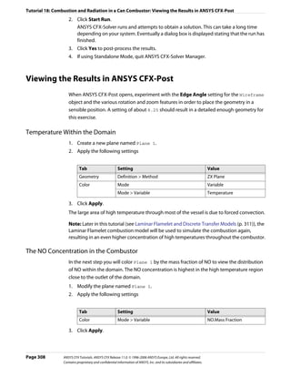
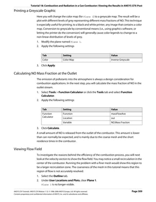
![Tutorial 18: Combustion and Radiation in a Can Combustor: Viewing the Results in ANSYS CFX-Post
3. Create a new vector named Vector 1.
4. Apply the following settings
Tab Setting Value
Geometry Definition > Locations Plane 1
Symbol Symbol Size 2
5. Click Apply.
6. Create a new plane named Plane 2.
7. Apply the following settings
Tab Setting Value
Geometry Definition > Method XY Plane
Definition > Z 0.03
Plane Bounds > Type Rectangular
Plane Bounds > X Size 0.5 [m]
Plane Bounds > Y Size 0.5 [m]
Plane Type > Sample (Selected)
Plane Type > X Samples 30
Plane Type > Y Samples 30
Render Draw Faces (Cleared)
8. Click Apply.
9. Modify Vector 1.
10. Apply the following setting
Tab Setting Value
Geometry Definition > Locations Plane 2
11. Click Apply.
To view the swirling velocity field, right-click in the viewer and select Predefined Camera >
View Towards -Z.
You may also want to turn off the wireframe visibility. In the region near the fuel and air
inlets, the swirl component of momentum (theta direction) results in increased mixing with
the surrounding fluid and a higher residence time in this region. As a result, more fuel is
burned.
Viewing Radiation
Try examining the distribution of Incident Radiation and Radiation Intensity
throughout the domain.
When you are finished, quit ANSYS CFX-Post.
Page 310 ANSYS CFX Tutorials. ANSYS CFX Release 11.0. © 1996-2006 ANSYS Europe, Ltd. All rights reserved.
Contains proprietary and confidential information of ANSYS, Inc. and its subsidiaries and affiliates.](https://image.slidesharecdn.com/ansys11tutorial-111218135319-phpapp01/85/Ansys-11-tutorial-322-320.jpg)
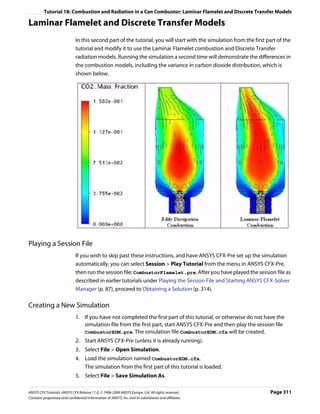
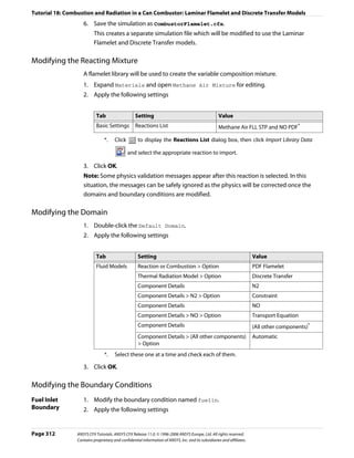
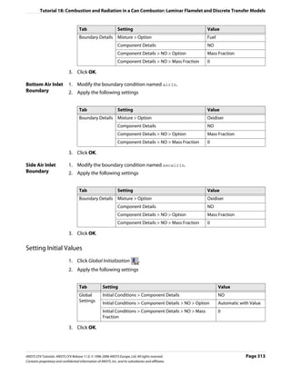

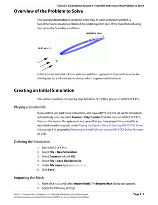
![Tutorial 19: Cavitation Around a Hydrofoil: Creating an Initial Simulation
Setting Value
File type CFX-Solver (*.def, *.ref, *.trn, *.bak)
File name HydrofoilGrid.def
3. Click Open.
4. Right-click a blank area in the viewer and select Predefined Camera > View Towards
-Z.
Loading Materials
Since this tutorial uses Water Vapour at 25 C and Water at 25 C you need to load these
materials.
1. In the Outline tree view, right-click Materials and select Import Library Data.
The Select Library Data to Import dialog box is displayed.
2. Expand Water Data.
3. Select both Water Vapour at 25 C and Water at 25 C by holding <Crtl> when
selecting.
4. Click OK.
Creating the Domain
The fluid domain used for this simulation contains liquid water and water vapour. The
volume fractions are initially set so that the domain is filled entirely with liquid.
1. Right click Simulation in the Outline tree view and ensure that Automatic Default
Domain is selected. A domain named Default Domain should now appear under the
Simulation branch.
2. Double click Default Domain and apply the following settings
Tab Setting Value
General Basic Settings > Fluids List * Water at 25 C, Water
Options Vapour at 25 C
Domain Models > Pressure > Reference Pressure 0 [atm]
Fluid Models Multiphase Options > Homogeneous Model (Selected)
Heat Transfer > Option Isothermal
Heat Transfer > Fluid Temperature 300 [K]
Turbulence > Option k-Epsilon
*. These two fluids have consistent reference enthalpies.
3. Click OK.
Creating the Boundary Conditions
The simulation requires inlet, outlet, wall and symmetry plane boundary conditions. The
regions for these boundary conditions were imported with the grid file.
Page 320 ANSYS CFX Tutorials. ANSYS CFX Release 11.0. © 1996-2006 ANSYS Europe, Ltd. All rights reserved.
Contains proprietary and confidential information of ANSYS, Inc. and its subsidiaries and affiliates.](https://image.slidesharecdn.com/ansys11tutorial-111218135319-phpapp01/85/Ansys-11-tutorial-332-320.jpg)
![Tutorial 19: Cavitation Around a Hydrofoil: Creating an Initial Simulation
Inlet Boundary 1. Create a new boundary condition named Inlet.
2. Apply the following settings
Tab Setting Value
Basic Settings Boundary Type Inlet
Location IN
Boundary Details Mass and Momentum > Normal Speed 16.91 [m s^-1]
Turbulence > Option Intensity and Length Scale
Turbulence > Value 0.03
Turbulence > Eddy Len. Scale 0.0076 [m]
Fluid Values Boundary Conditions Water at 25 C
Boundary Conditions > Water at 25 C> 1
Volume Fraction > Volume Fraction
Boundary Conditions Water Vapour at 25 C
Boundary Conditions > Water Vapour at 25 C > 0
Volume Fraction > Volume Fraction
3. Click OK.
Outlet 1. Create a new boundary condition named Outlet.
Boundary 2. Apply the following settings
Tab Setting Value
Basic Settings Boundary Type Outlet
Location OUT
Boundary Details Mass and Momentum > Option Static Pressure
Mass and Momentum > Relative Pressure 51957 [Pa]
3. Click OK.
Free Slip Wall 1. Create a new boundary condition named SlipWalls.
Boundary 2. Apply the following settings
Tab Setting Value
Basic Settings Boundary Type Wall
Location BOT, TOP
Boundary Details Wall Influence on Flow > Option Free Slip
3. Click OK.
Symmetry Plane 1. Create a new boundary condition named Sym1.
Boundaries 2. Apply the following settings
ANSYS CFX Tutorials. ANSYS CFX Release 11.0. © 1996-2006 ANSYS Europe, Ltd. All rights reserved. Page 321
Contains proprietary and confidential information of ANSYS, Inc. and its subsidiaries and affiliates.](https://image.slidesharecdn.com/ansys11tutorial-111218135319-phpapp01/85/Ansys-11-tutorial-333-320.jpg)
![Tutorial 19: Cavitation Around a Hydrofoil: Creating an Initial Simulation
Tab Setting Value
Basic Settings Boundary Type Symmetry
Location SYM1
3. Click OK.
1. Create a new boundary condition named Sym2.
2. Apply the following settings
Tab Setting Value
Basic Settings Boundary Type Symmetry
Location SYM2
3. Click OK.
Setting Initial Values
1. Click Global Initialization .
2. Apply the following settings
Tab Setting Value
Global Initial Conditions > Cartesian Velocity Components > Automatic with Value
Settings Option
Initial Conditions > Cartesian Velocity Components > U 16.91 [m s^-1]
Initial Conditions > Cartesian Velocity Components > V 0 [m s^-1]
Initial Conditions > Cartesian Velocity Components > W 0 [m s^-1]
Initial Conditions > Turbulence Eddy Dissipation (Selected)
Fluid Fluid Specific Initialization Water
Settings at 25 C
Fluid Specific Initialization > Water at 25 C (Selected)
Fluid Specific Initialization > Water at 25 C > Initial Automatic with Value
Conditions > Volume Fraction > Option
Fluid Specific Initialization > Water at 25 C > Initial 1
Conditions > Volume Fraction > Volume Fraction
Fluid Specific Initialization Water Vapour at 25 C
Fluid Specific Initialization > Water Vapour at 25 C (Selected)
Fluid Specific Initialization > Water Vapour at 25 C > Initial Automatic with Value
Conditions > Volume Fraction > Option
Fluid Specific Initialization > Water Vapour at 25 C > Initial 0
Conditions > Volume Fraction > Volume Fraction
3. Click OK.
Page 322 ANSYS CFX Tutorials. ANSYS CFX Release 11.0. © 1996-2006 ANSYS Europe, Ltd. All rights reserved.
Contains proprietary and confidential information of ANSYS, Inc. and its subsidiaries and affiliates.](https://image.slidesharecdn.com/ansys11tutorial-111218135319-phpapp01/85/Ansys-11-tutorial-334-320.jpg)
![Tutorial 19: Cavitation Around a Hydrofoil: Obtaining an Initial Solution using ANSYS CFX-Solver Manager
Setting Solver Control
1. Click Solver Control .
2. Apply the following settings
Tab Setting Value
Basic Settings Convergence Control > Max. Iterations 35
Convergence Control > Fluid Timescale Physical Timescale
Control > Timescale Control
Convergence Control > Fluid Timescale 0.01 [s]
Control > Physical Timescale
Note: For the Convergence Criteria, an RMS value of at least 1e-05 is usually required for
adequate convergence, but the default value is sufficient for demonstration purposes.
3. Click OK.
Writing the Solver (.def) File
1. Click Write Solver File .
2. Apply the following settings
Setting Value
File name HydrofoilIni.def
Quit CFX–Pre * (Selected)
*. If using ANSYS CFX-Pre in Standalone Mode.
3. Ensure Start Solver Manager is selected and click Save.
4. Quit ANSYS CFX-Pre, saving the simulation (.cfx) file at your discretion.
Obtaining an Initial Solution using ANSYS CFX-Solver Manager
While the calculations proceed, you can see residual output for various equations in both
the text area and the plot area. Use the tabs to switch between different plots (e.g.,
Momentum and Mass, Turbulence Quantities, etc.) in the plot area. You can view residual
plots for the fluid and solid domains separately by editing the workspace properties.
1. Ensure that the Define Run dialog box is displayed.
2. Click Start Run.
ANSYS CFX-Solver runs and attempts to obtain a solution. This can take a long time
depending on your system. Eventually a dialog box is displayed.
3. Click Yes to post-process the results.
4. If using Standalone Mode, quit ANSYS CFX-Solver Manager.
ANSYS CFX Tutorials. ANSYS CFX Release 11.0. © 1996-2006 ANSYS Europe, Ltd. All rights reserved. Page 323
Contains proprietary and confidential information of ANSYS, Inc. and its subsidiaries and affiliates.](https://image.slidesharecdn.com/ansys11tutorial-111218135319-phpapp01/85/Ansys-11-tutorial-335-320.jpg)
![Tutorial 19: Cavitation Around a Hydrofoil: Viewing the Results of the Initial Simulation
Viewing the Results of the Initial Simulation
The following topics will be discussed:
• Plotting Pressure Distribution Data (p. 324)
• Exporting Pressure Distribution Data (p. 325)
• Saving the Post-Processing State (p. 326)
Plotting Pressure Distribution Data
In this section, you will create a plot of the pressure coefficient distribution around the
hydrofoil. The data will then be exported to a file for later comparison with data from the
cavitating flow case, which will be run later in this tutorial.
1. Right-click a blank area in the viewer and select Predefined Camera > View Towards
-Z.
2. Insert a new plane named Slice.
3. Apply the following settings
Tab Setting Value
Geometry Definition > Method XY Plane
Definition > Z 5e-5 [m]
Render Draw Faces (Cleared)
4. Click Apply.
5. Create a new polyline named Foil by selecting Insert > Location > Polyline from the
main menu.
6. Apply the following settings
Tab Setting Value
Geometry Method Boundary Intersection
Boundary List Default Domain Default
Intersect With Slice
7. Click Apply.
Zoom in on the center of the hydrofoil (near the cavity) to confirm the polyline wraps
around the hydrofoil.
8. Create a new variable named Pressure Coefficient.
9. Apply the following settings
Setting Value
Expression (Pressure-51957[Pa])/(0.5*996.2[kg m^-3]*16.91[m s^-1]^2)
10. Click Apply.
11. Create a new variable named Chord.
12. Apply the following settings
Page 324 ANSYS CFX Tutorials. ANSYS CFX Release 11.0. © 1996-2006 ANSYS Europe, Ltd. All rights reserved.
Contains proprietary and confidential information of ANSYS, Inc. and its subsidiaries and affiliates.](https://image.slidesharecdn.com/ansys11tutorial-111218135319-phpapp01/85/Ansys-11-tutorial-336-320.jpg)

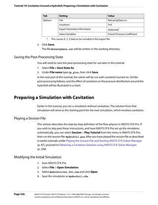
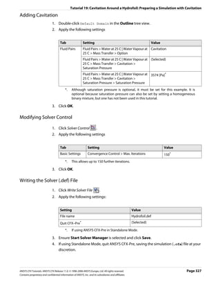
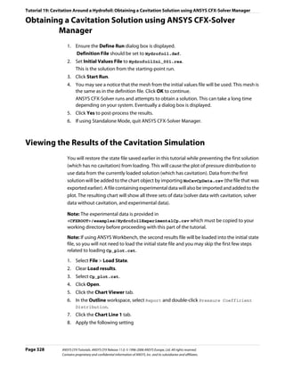
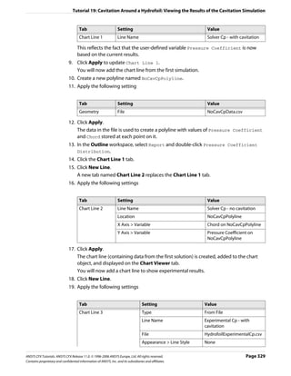
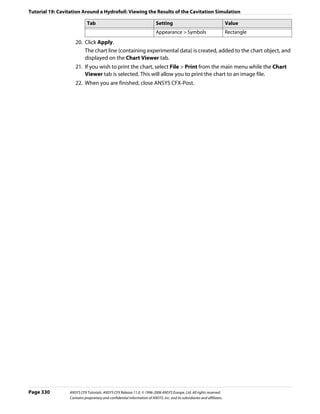


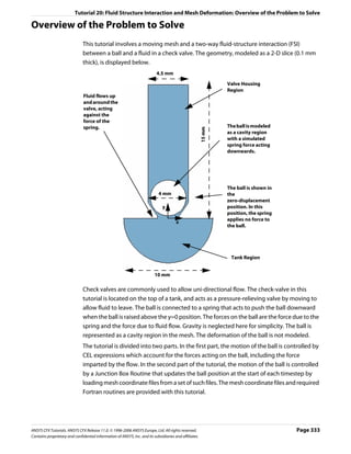


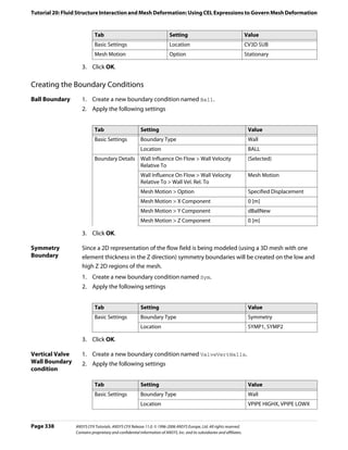
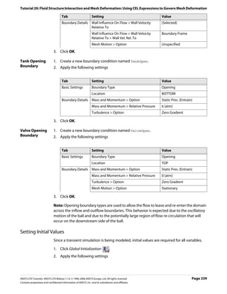
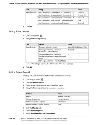
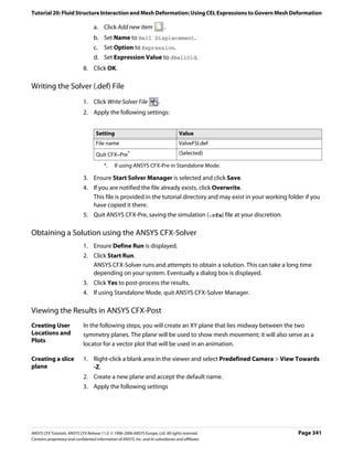

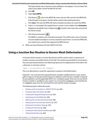
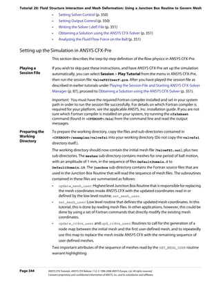

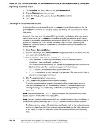
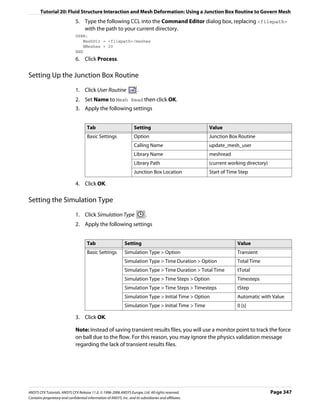
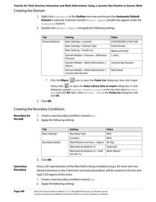

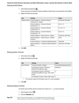


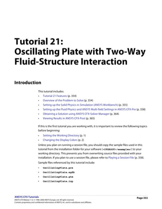
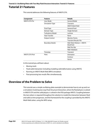

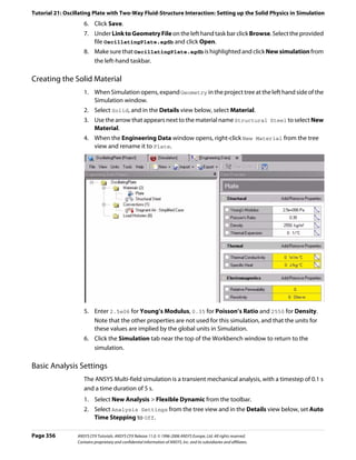
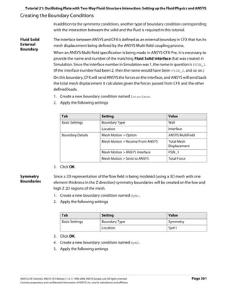

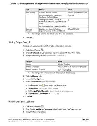
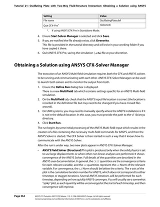

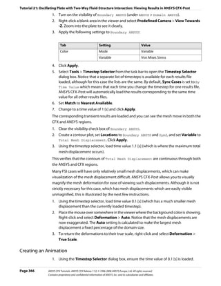
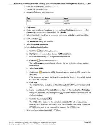
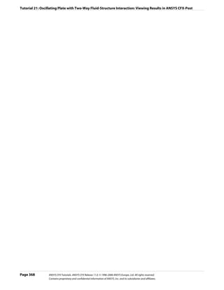
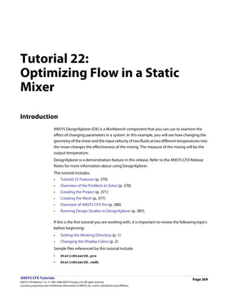
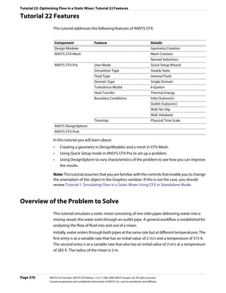
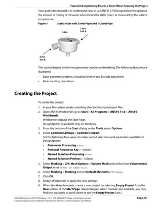

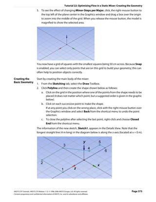

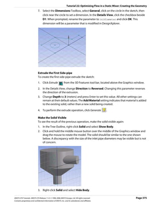
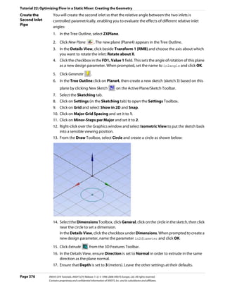
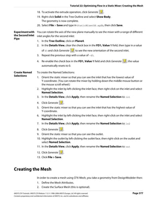
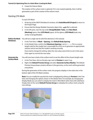
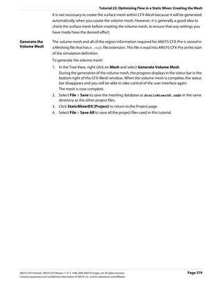
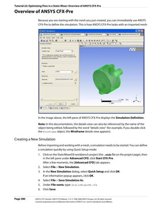
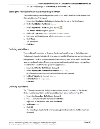
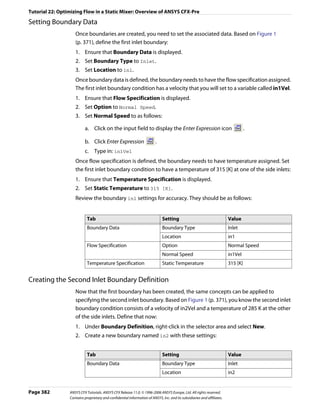

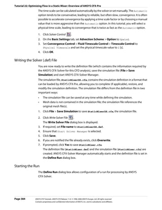
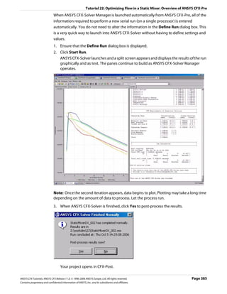
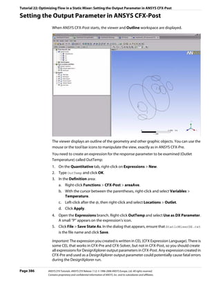
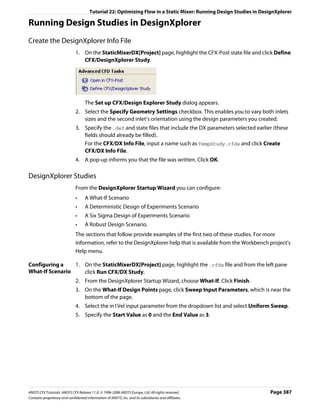
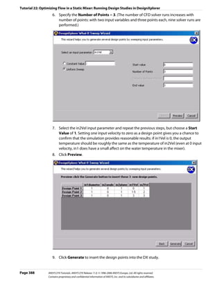
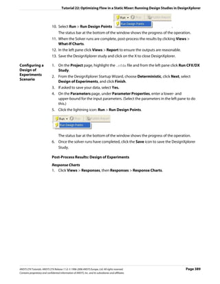
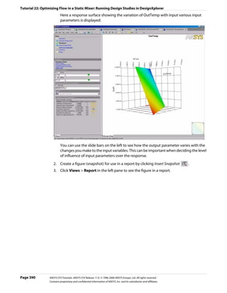
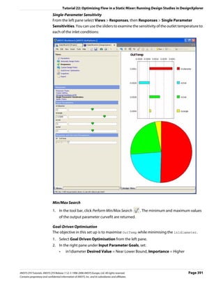
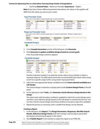


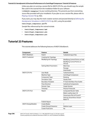
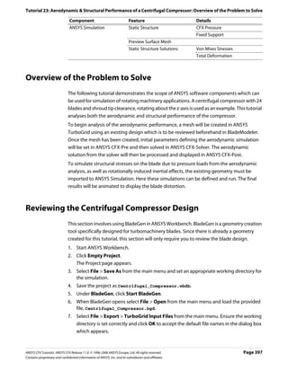
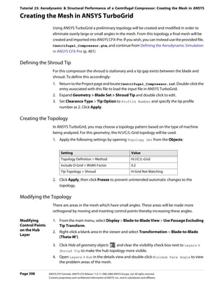
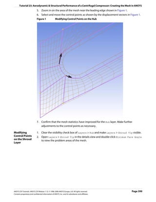
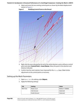
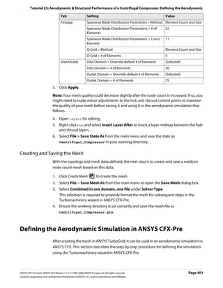


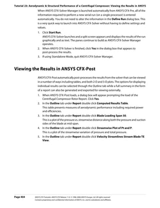
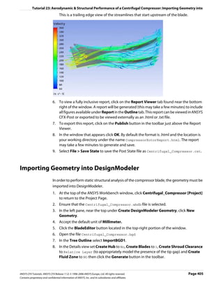

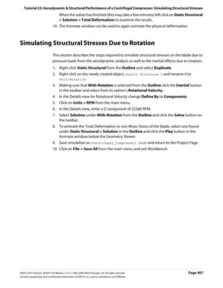

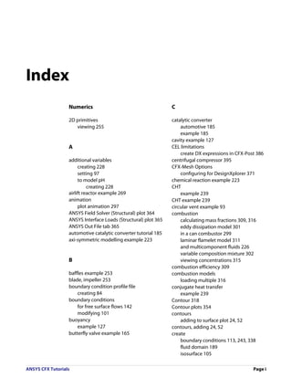
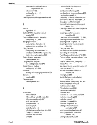
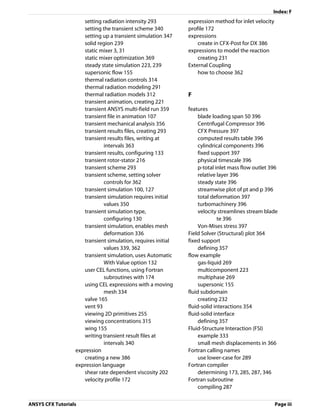

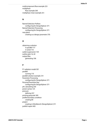


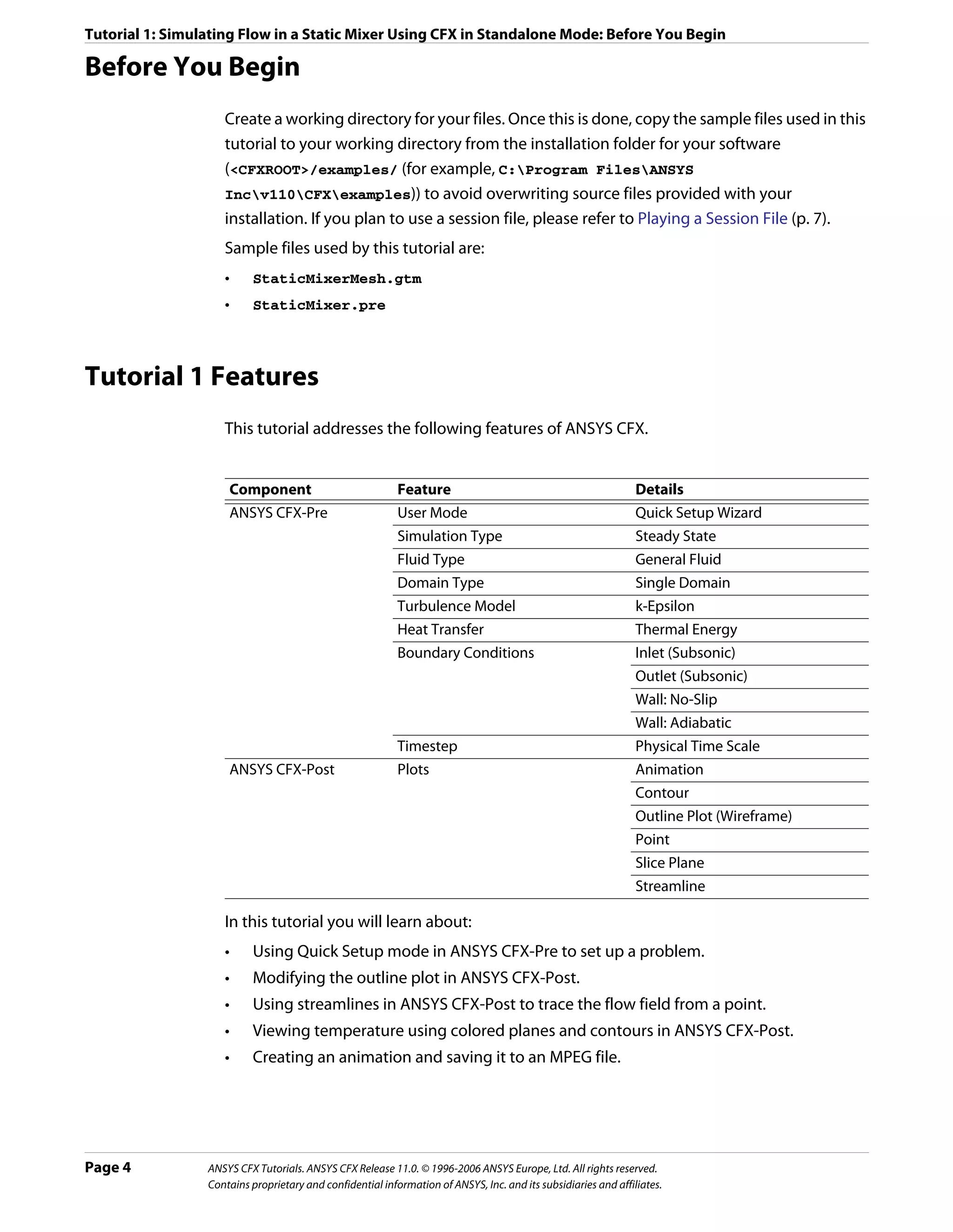
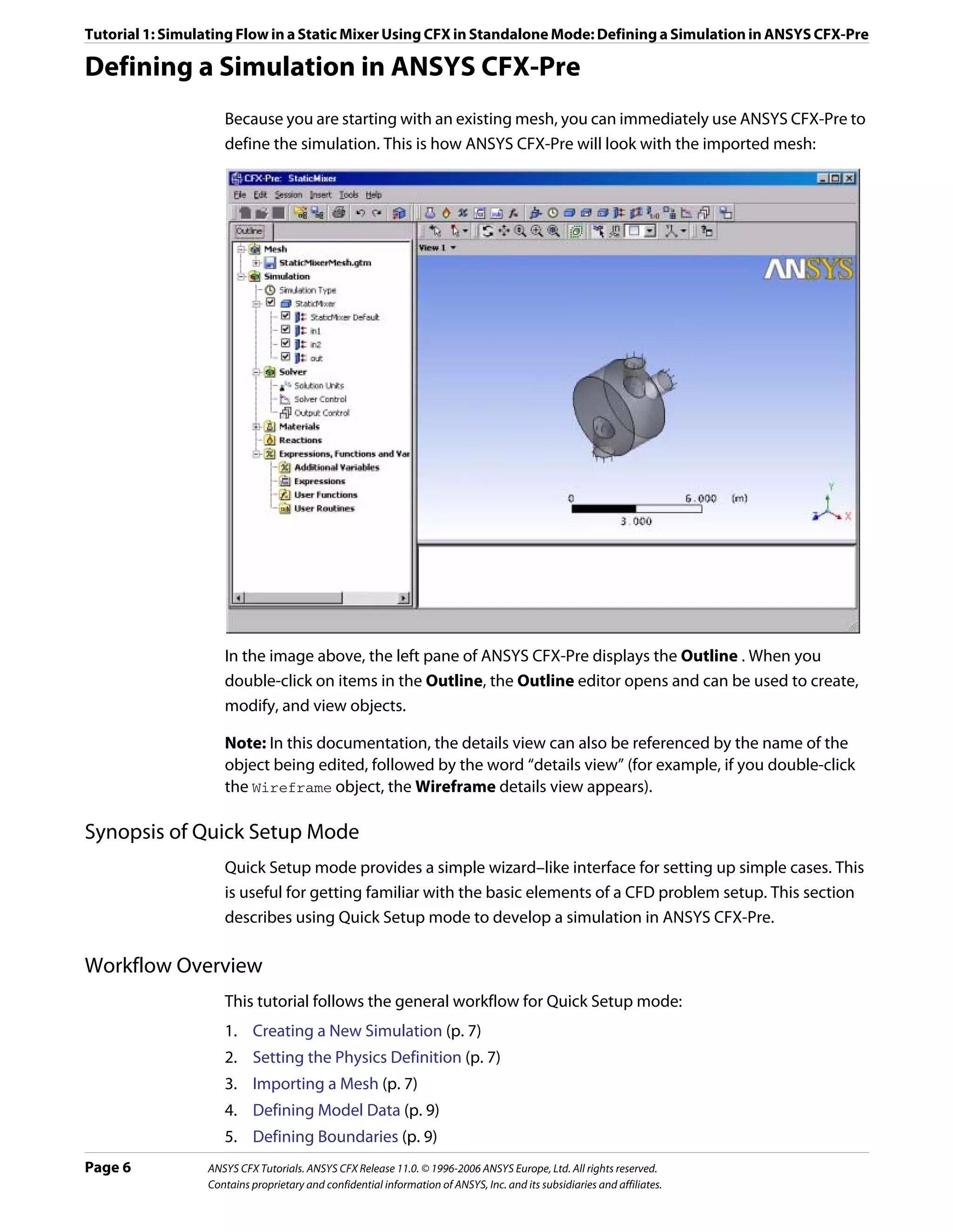

![Tutorial 1: Simulating Flow in a Static Mixer Using CFX in Standalone Mode: Defining a Simulation in ANSYS CFX-Pre
Defining Model Data
You need to define the type of flow and the physical models to use in the fluid domain.
You will specify the flow as steady state with turbulence and heat transfer. Turbulence is
modeled using the k - ε turbulence model and heat transfer using the thermal energy
model. The k - ε turbulence model is a commonly used model and is suitable for a wide
range of applications. The thermal energy model neglects high speed energy effects and is
therefore suitable for low speed flow applications.
Procedure 1. Ensure that Physics Definition is displayed.
2. Under Model Data, set Reference Pressure to 1 [atm].
All other pressure settings are relative to this reference pressure.
3. Set Heat Transfer to Thermal Energy.
4. Set Turbulence to k-Epsilon.
5. Click Next.
Defining Boundaries
The CFD model requires the definition of conditions on the boundaries of the domain.
Procedure 1. Ensure that Boundary Definition is displayed.
2. Delete Inlet and Outlet from the list by right-clicking each and selecting Delete.
3. Right-click in the blank area where Inlet and Outlet were listed, then select New.
4. Set Name to in1.
5. Click OK.
The boundary is created and, when selected, properties related to the boundary are
displayed.
Setting Boundary Data
Once boundaries are created, you need to create associated data. Based on Figure 1, you will
define the first inlet boundary condition’s velocity and temperature.
Procedure 1. Ensure that Boundary Data is displayed.
2. Set Boundary Type to Inlet.
3. Set Location to in1.
Setting Flow Specification
Once boundary data is defined, the boundary needs to have the flow specification assigned.
Procedure 1. Ensure that Flow Specification is displayed.
2. Set Option to Normal Speed.
3. Set Normal Speed to 2 [m s^-1].
ANSYS CFX Tutorials. ANSYS CFX Release 11.0. © 1996-2006 ANSYS Europe, Ltd. All rights reserved. Page 9
Contains proprietary and confidential information of ANSYS, Inc. and its subsidiaries and affiliates.](https://image.slidesharecdn.com/ansys11tutorial-111218135319-phpapp01/75/Ansys-11-tutorial-21-2048.jpg)
![Tutorial 1: Simulating Flow in a Static Mixer Using CFX in Standalone Mode: Defining a Simulation in ANSYS CFX-Pre
Setting Temperature Specification
Once flow specification is defined, the boundary needs to have temperature assigned.
Procedure 1. Ensure that Temperature Specification is displayed.
2. Set Static Temperature to 315 [K].
Reviewing the Boundary Condition Definitions
Defining the boundary condition for in1 required several steps. Here the settings are
reviewed for accuracy.
Based on Figure 1, the first inlet boundary condition consists of a velocity of 2 m/s and a
temperature of 315 K at one of the side inlets.
Procedure 1. Review the boundary in1 settings for accuracy. They should be as follows:
Tab Setting Value
Boundary Data Boundary Type Inlet
Location in1
Flow Specification Option Normal Speed
Normal Speed 2 [m s^-1]
Temperature Specification Static Temperature 315 [K]
Creating the Second Inlet Boundary Definition
Based on Figure 1, you know the second inlet boundary condition consists of a velocity of 2
m/s and a temperature of 285 K at one of the side inlets. You will define that now.
Procedure 1. Under Boundary Definition, right-click in the selector area and select New.
2. Create a new boundary named in2 with these settings:
Tab Setting Value
Boundary Data Boundary Type Inlet
Location in2
Flow Specification Option Normal Speed
Normal Speed 2 [m s^-1]
Temperature Specification Static Temperature 285 [K]
Creating the Outlet Boundary Definition
Now that the second inlet boundary has been created, the same concepts can be applied to
building the outlet boundary.
1. Create a new boundary named out with these settings:
Page 10 ANSYS CFX Tutorials. ANSYS CFX Release 11.0. © 1996-2006 ANSYS Europe, Ltd. All rights reserved.
Contains proprietary and confidential information of ANSYS, Inc. and its subsidiaries and affiliates.](https://image.slidesharecdn.com/ansys11tutorial-111218135319-phpapp01/75/Ansys-11-tutorial-22-2048.jpg)
![Tutorial 1: Simulating Flow in a Static Mixer Using CFX in Standalone Mode: Defining a Simulation in ANSYS CFX-Pre
Tab Setting Value
Boundary Data Boundary Type Outlet
Location out
Flow Specification Option Average Static Pressure
Relative Pressure 0 [Pa]
2. Click Next.
Moving to General Mode
There are no further boundary conditions that need to be set. All 2D exterior regions that
have not been assigned to a boundary condition are automatically assigned to the default
boundary condition.
Procedure 1. Set Operation to Enter General Mode and click Finish.
The three boundary conditions are displayed in the viewer as sets of arrows at the
boundary surfaces. Inlet boundary arrows are directed into the domain. Outlet
boundary arrows are directed out of the domain.
Setting Solver Control
Solver Control parameters control aspects of the numerical solution generation process.
While an upwind advection scheme is less accurate than other advection schemes, it is also
more robust. This advection scheme is suitable for obtaining an initial set of results, but in
general should not be used to obtain final accurate results.
The time scale can be calculated automatically by the solver or set manually. The Automatic
option tends to be conservative, leading to reliable, but often slow, convergence. It is often
possible to accelerate convergence by applying a time scale factor or by choosing a manual
value that is more aggressive than the Automatic option. In this tutorial, you will select a
physical time scale, leading to convergence that is twice as fast as the Automatic option.
Procedure 1. Click Solver Control .
2. On the Basic Settings tab, set Advection Scheme > Option to Upwind.
3. Set Convergence Control > Fluid Timescale Control > Timescale Control to
Physical Timescale and set the physical timescale value to 2 [s].
4. Click OK.
Writing the Solver (.def) File
The simulation file, StaticMixer.cfx, contains the simulation definition in a format that
can be loaded by ANSYS CFX-Pre, allowing you to complete (if applicable), restore, and
modify the simulation definition. The simulation file differs from the definition file in that it
can be saved at any time while defining the simulation.
Procedure 1. Click Write Solver File .
ANSYS CFX Tutorials. ANSYS CFX Release 11.0. © 1996-2006 ANSYS Europe, Ltd. All rights reserved. Page 11
Contains proprietary and confidential information of ANSYS, Inc. and its subsidiaries and affiliates.](https://image.slidesharecdn.com/ansys11tutorial-111218135319-phpapp01/75/Ansys-11-tutorial-23-2048.jpg)
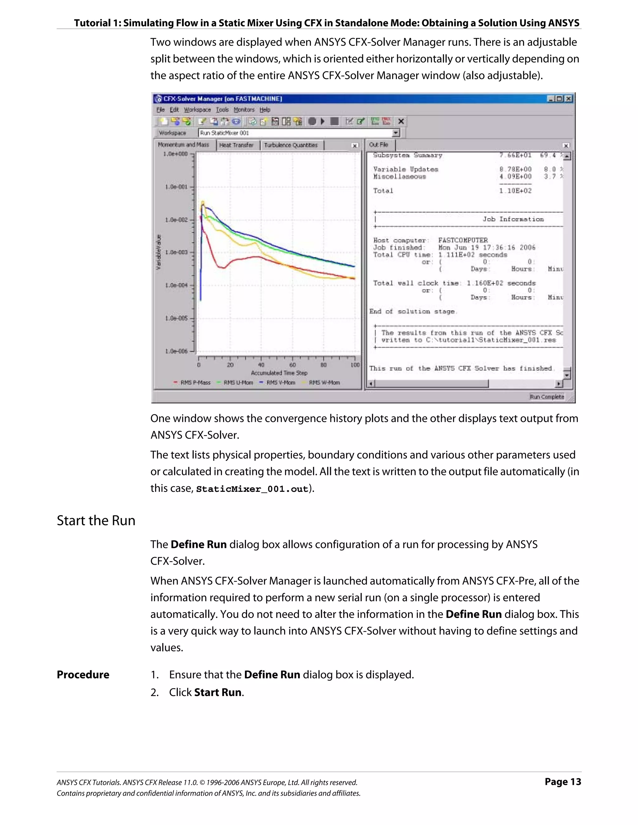
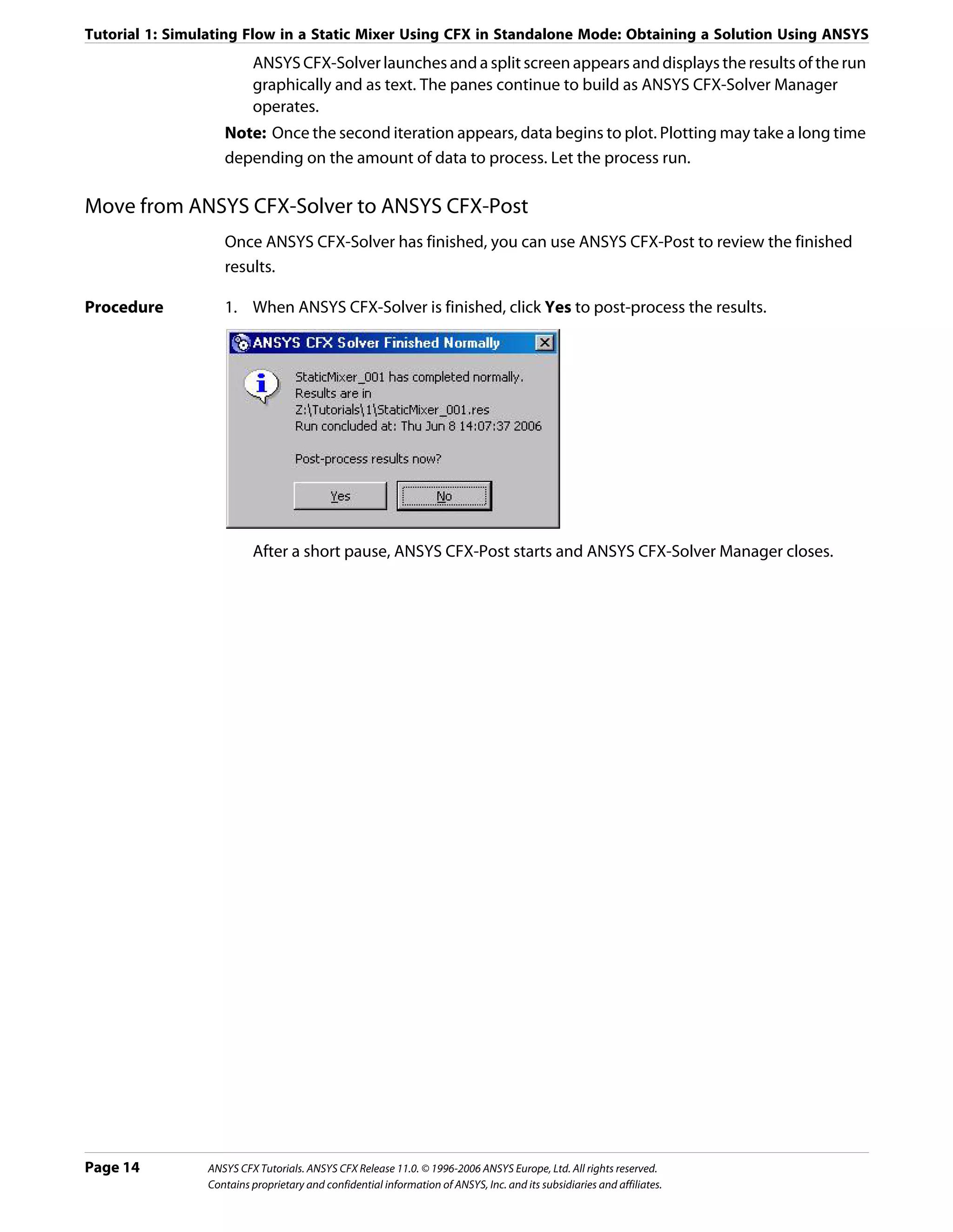

![Tutorial 1: Simulating Flow in a Static Mixer Using CFX in Standalone Mode: Viewing the Results in ANSYS CFX-Post
15. Creating the First Keyframe (p. 26)
16. Creating the Second Keyframe (p. 26)
17. Viewing the Animation (p. 27)
18. Modifying the Animation (p. 28)
19. Saving to MPEG (p. 29)
Setting the Edge Angle for a Wireframe Object
The outline of the geometry is called the wireframe or outline plot.
By default, ANSYS CFX-Post displays only some of the surface mesh. This sometimes means
that when you first load your results file, the geometry outline is not displayed clearly. You
can control the amount of the surface mesh shown by editing the Wireframe object listed
in the Outline.
The check boxes next to each object name in the Outline control the visibility of each
object. Currently only the Wireframe and Default Legend objects have visibility selected.
The edge angle determines how much of the surface mesh is visible. If the angle between
two adjacent faces is greater than the edge angle, then that edge is drawn. If the edge angle
is set to 0°, the entire surface mesh is drawn. If the edge angle is large, then only the most
significant corner edges of the geometry are drawn.
For this geometry, a setting of approximately 15° lets you view the model location without
displaying an excessive amount of the surface mesh.
In this module you can also modify the zoom settings and view of the wireframe.
Procedure 1. In the Outline, under User Locations and Plots, double-click Wireframe.
Tip: While it is not necessary to change the view to set the angle, do so to explore the
practical uses of this feature.
2. Right-click on a blank area anywhere in the viewer, select Predefined Camera from the
shortcut menu and select Isometric View (Z up).
3. In the Wireframe details view, under Definition, click in the Edge Angle box.
An embedded slider is displayed.
4. Type a value of 10 [degree].
5. Click Apply to update the object with the new setting.
Page 16 ANSYS CFX Tutorials. ANSYS CFX Release 11.0. © 1996-2006 ANSYS Europe, Ltd. All rights reserved.
Contains proprietary and confidential information of ANSYS, Inc. and its subsidiaries and affiliates.](https://image.slidesharecdn.com/ansys11tutorial-111218135319-phpapp01/75/Ansys-11-tutorial-28-2048.jpg)
![Tutorial 1: Simulating Flow in a Static Mixer Using CFX in Standalone Mode: Viewing the Results in ANSYS CFX-Post
Notice that more surface mesh is displayed.
6. Drag the embedded slider to set the Edge Angle value to approximately 45 [degree].
7. Click Apply to update the object with the new setting.
Less of the outline of the geometry is displayed.
8. Type a value of 15 [degree].
9. Click Apply to update the object with the new setting.
10. Right-click on a blank area anywhere in the viewer, select Predefined Camera from the
shortcut menu and select View Towards -X.
Creating a Point for the Origin of the Streamline
A streamline is the path that a particle of zero mass would follow through the domain.
Procedure 1. Select Insert > Location > Point from the main menu.
You can also use the toolbars to create a variety of objects. Later modules and tutorials
explore this further.
2. Click OK.
This accepts the default name.
3. Under Definition, ensure that Method is set to XYZ.
4. Under Point, enter the following coordinates: -1, -1, 1.
This is a point near the first inlet.
5. Click Apply.
The point appears as a symbol in the viewer as a crosshair symbol.
ANSYS CFX Tutorials. ANSYS CFX Release 11.0. © 1996-2006 ANSYS Europe, Ltd. All rights reserved. Page 17
Contains proprietary and confidential information of ANSYS, Inc. and its subsidiaries and affiliates.](https://image.slidesharecdn.com/ansys11tutorial-111218135319-phpapp01/75/Ansys-11-tutorial-29-2048.jpg)
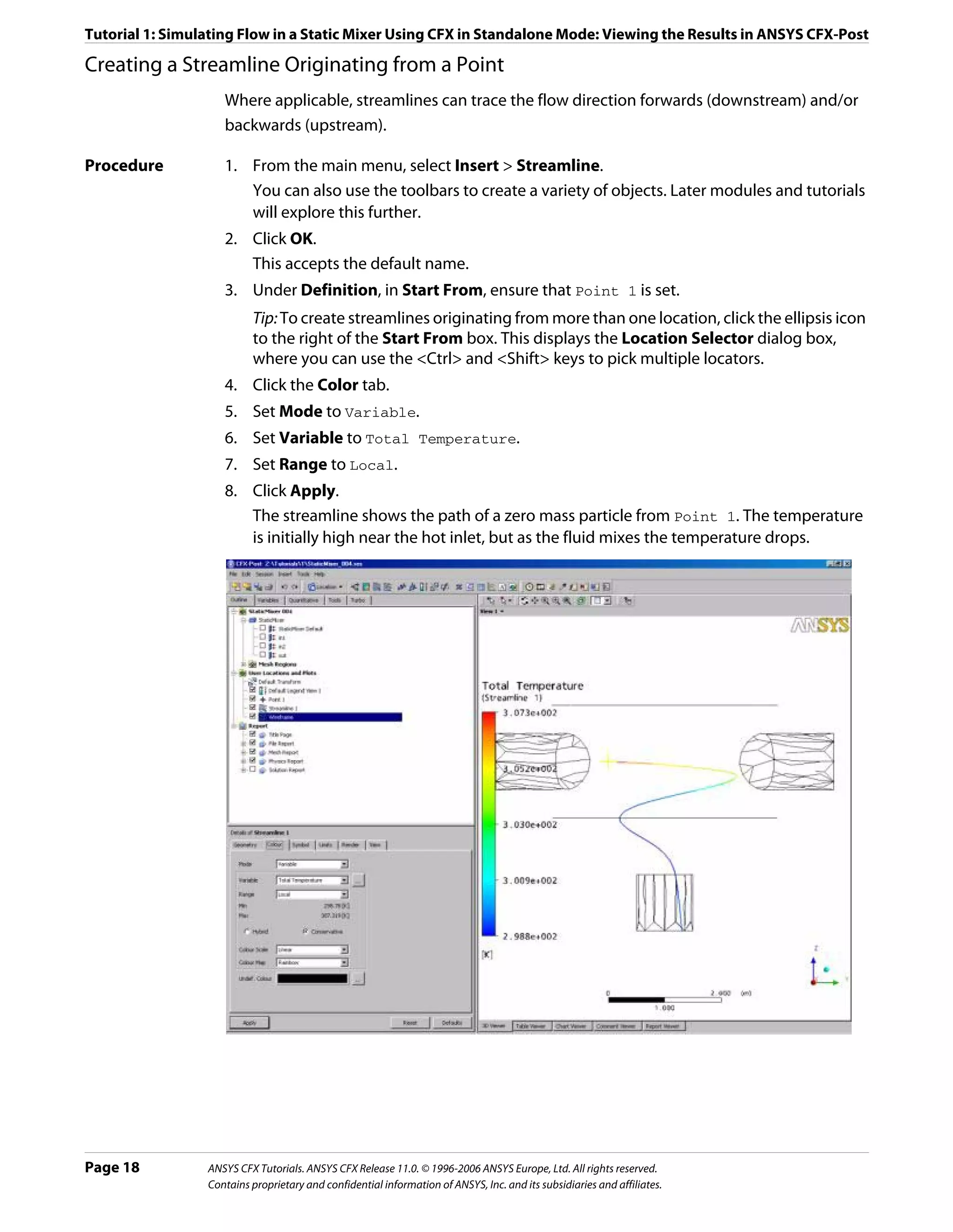
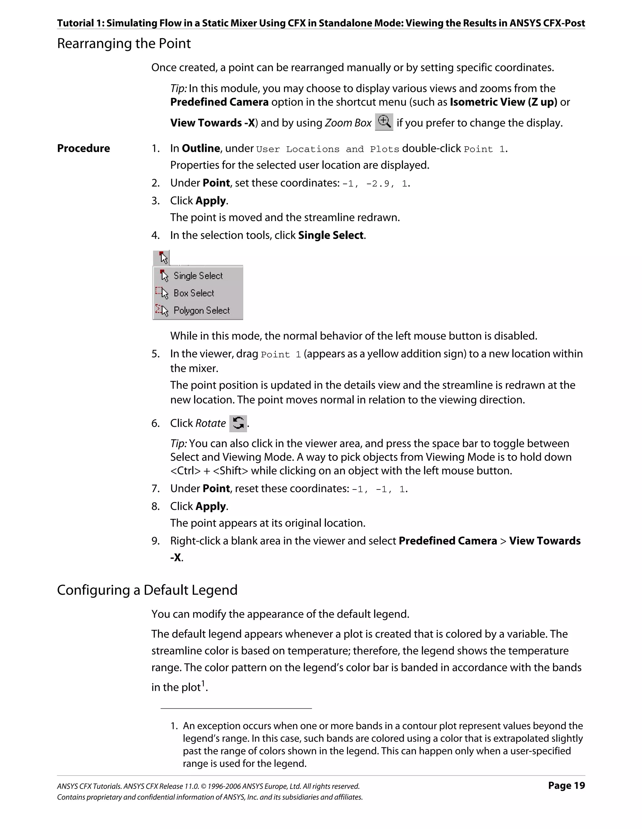
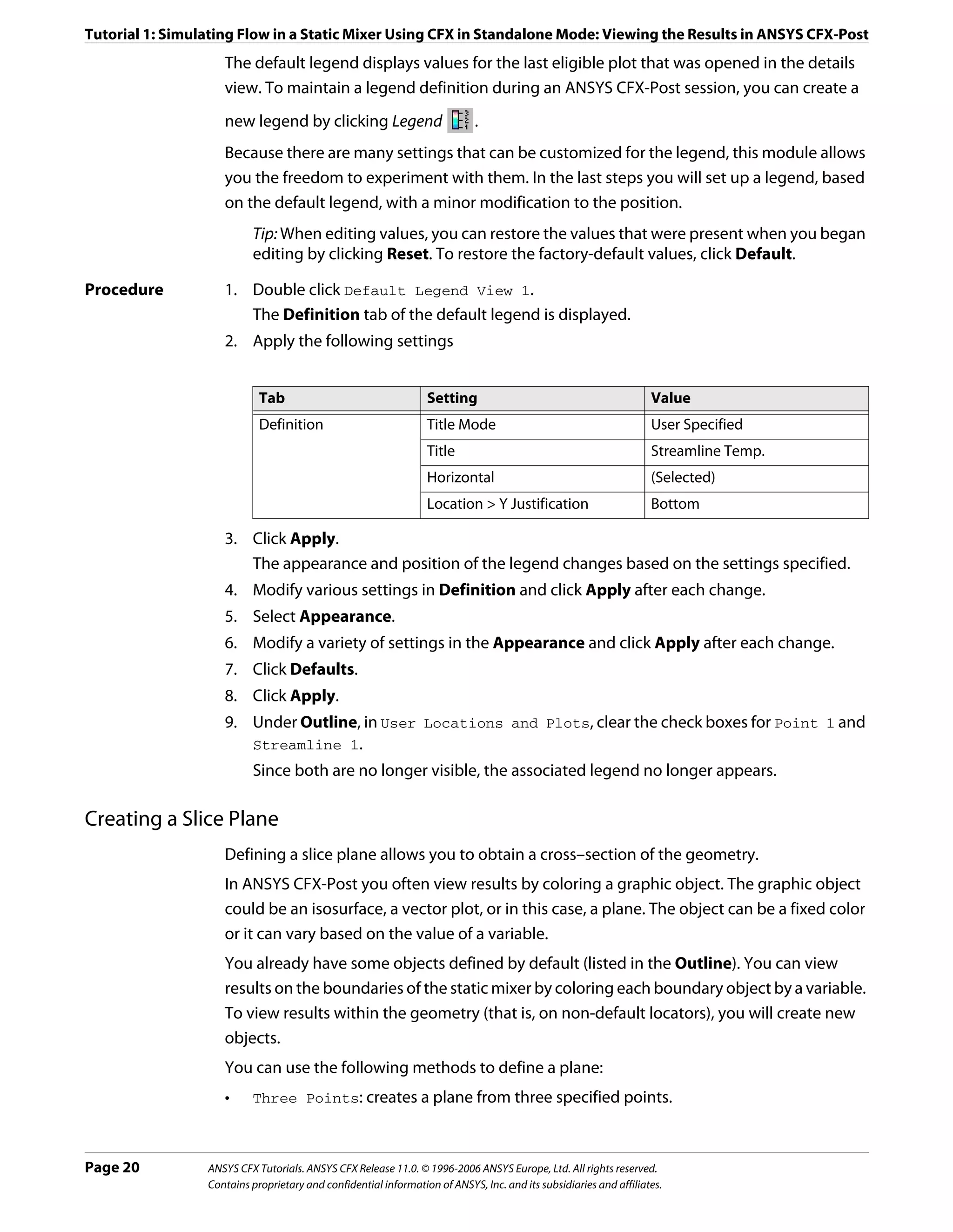

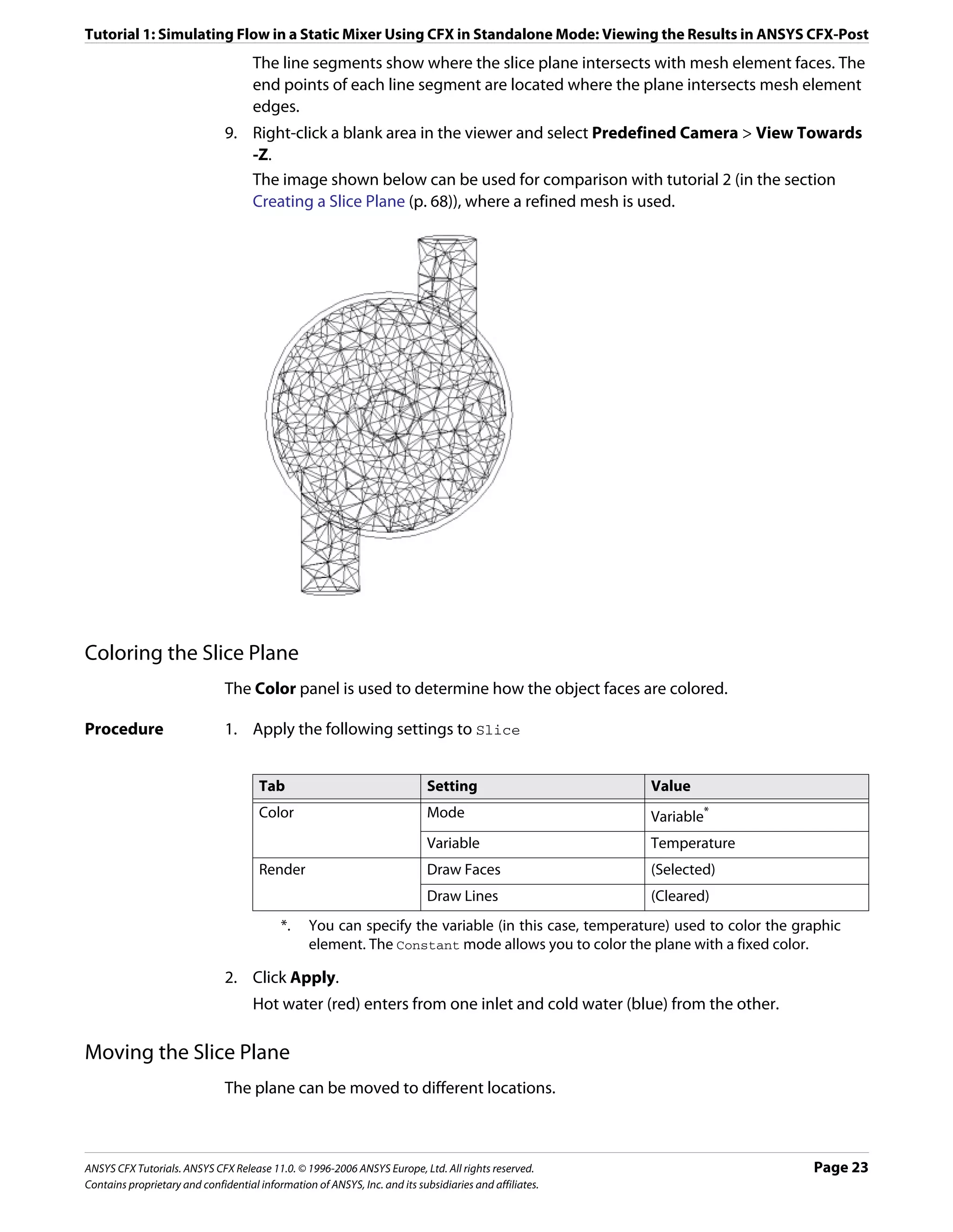

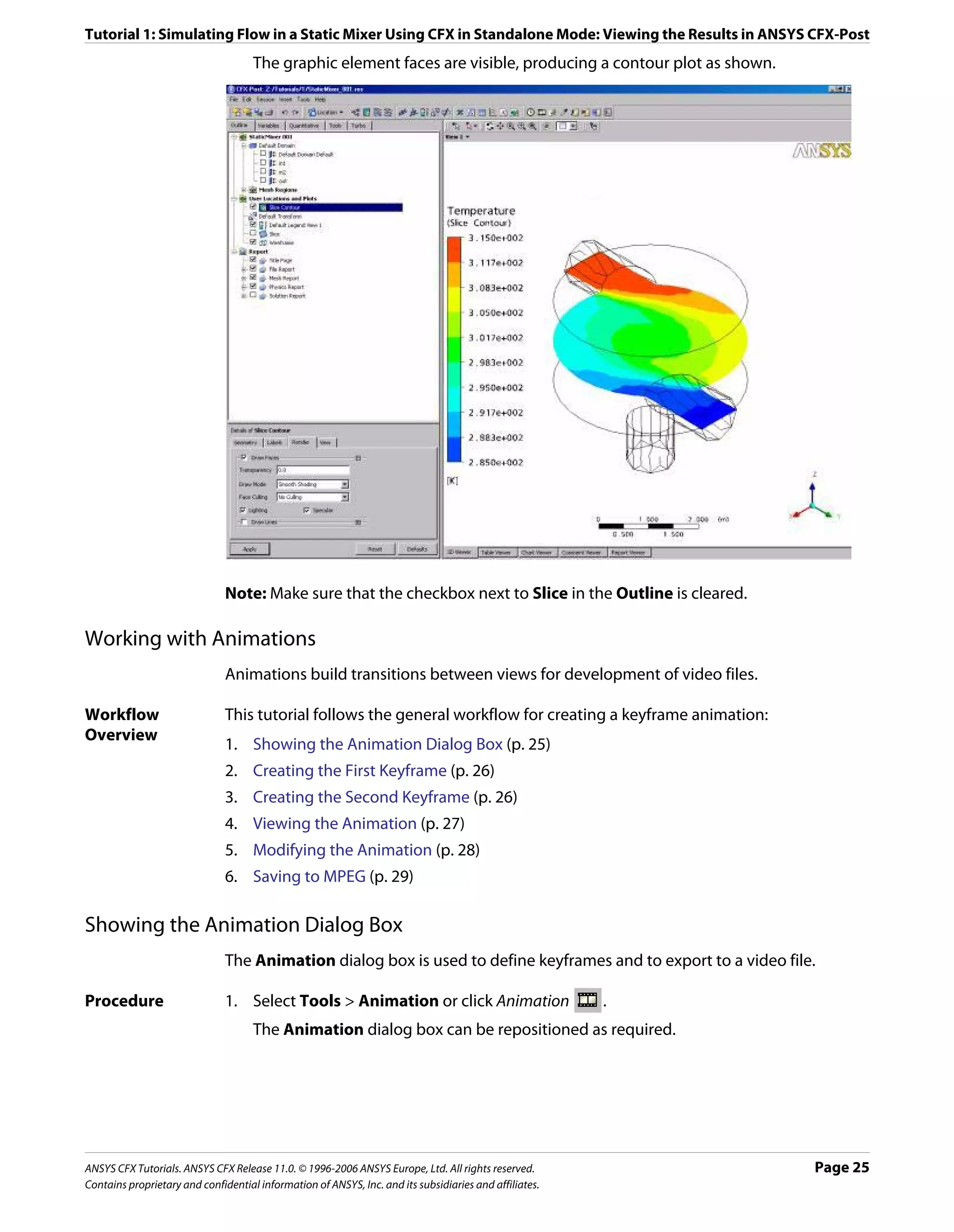
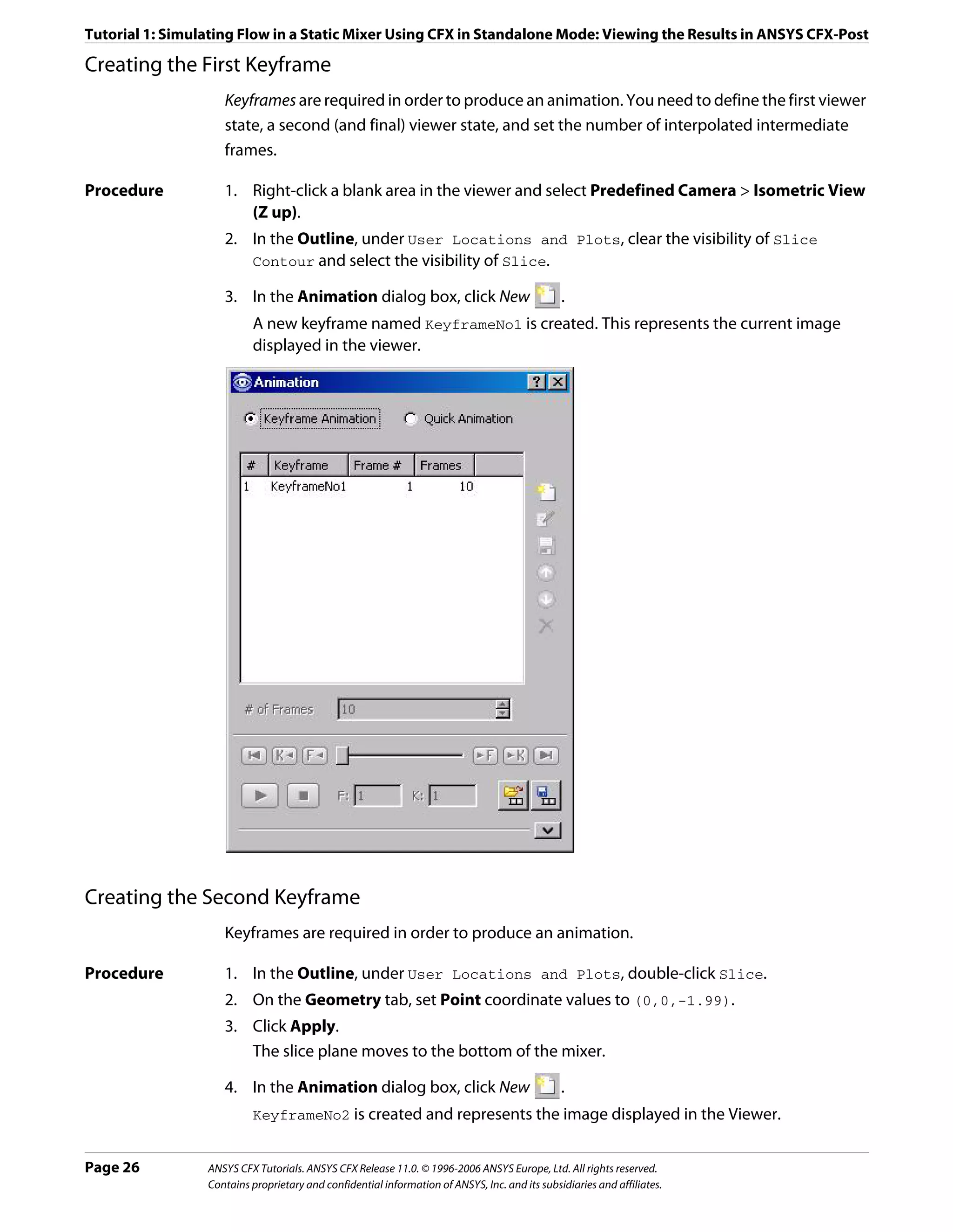
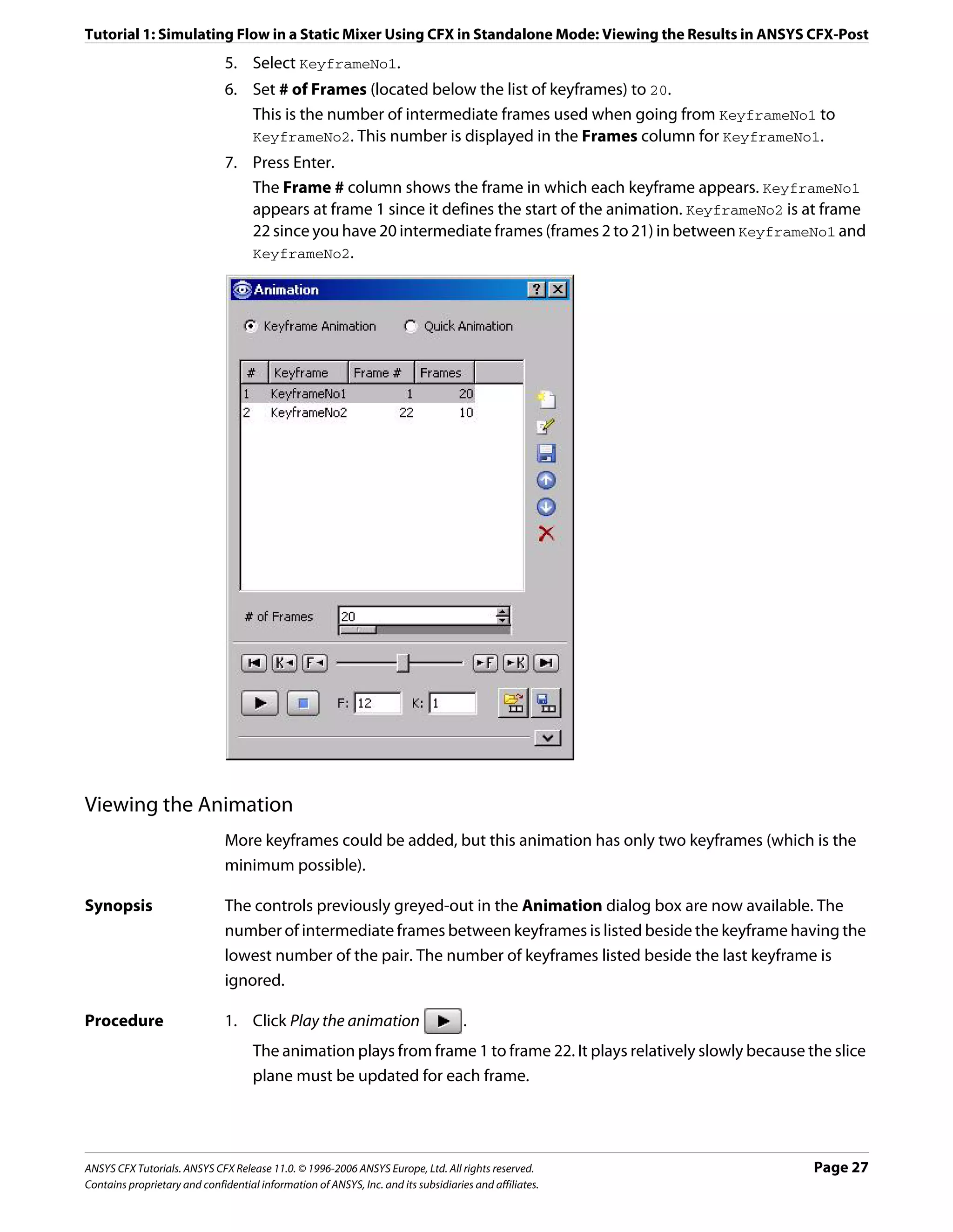
![Tutorial 1: Simulating Flow in a Static Mixer Using CFX in Standalone Mode: Viewing the Results in ANSYS CFX-Post
Modifying the Animation
To make the plane sweep through the whole geometry, you will set the starting position of
the plane to be at the top of the mixer. You will also modify the Range properties of the
plane so that it shows the temperature variation better. As the animation is played, you can
see the hot and cold water entering the mixer. Near the bottom of the mixer (where the
water flows out) you can see that the temperature is quite uniform. The new temperature
range lets you view the mixing process more accurately than the global range used in the
first animation.
Procedure 1. Apply the following settings to Slice
Tab Setting Value
Geometry Point 0, 0, 1.99
Color Variable Temperature
Range User Specified
Min 295 [K]
Max 305 [K]
2. Click Apply.
The slice plane moves to the top of the static mixer.
Note: Do not double click in the next step.
3. In the Animation dialog box, single click (do not double-click) KeyframeNo1 to select it.
If you had double-clicked KeyFrameNo1, the plane and viewer states would have been
redefined according to the stored settings for KeyFrameNo1. If this happens, click
Undo and try again to select the keyframe.
4. Click Set Keyframe .
The image in the Viewer replaces the one previously associated with KeyframeNo1.
5. Double-click KeyframeNo2.
The object properties for the slice plane are updated according to the settings in
KeyFrameNo2.
6. Apply the following settings to Slice
Tab Setting Value
Color Variable Temperature
Range User Specified
Min 295 [K]
Max 305 [K]
7. Click Apply.
8. In the Animation dialog box, single-click KeyframeNo2.
9. Click Set Keyframe to save the new settings to KeyframeNo2.
Page 28 ANSYS CFX Tutorials. ANSYS CFX Release 11.0. © 1996-2006 ANSYS Europe, Ltd. All rights reserved.
Contains proprietary and confidential information of ANSYS, Inc. and its subsidiaries and affiliates.](https://image.slidesharecdn.com/ansys11tutorial-111218135319-phpapp01/75/Ansys-11-tutorial-40-2048.jpg)
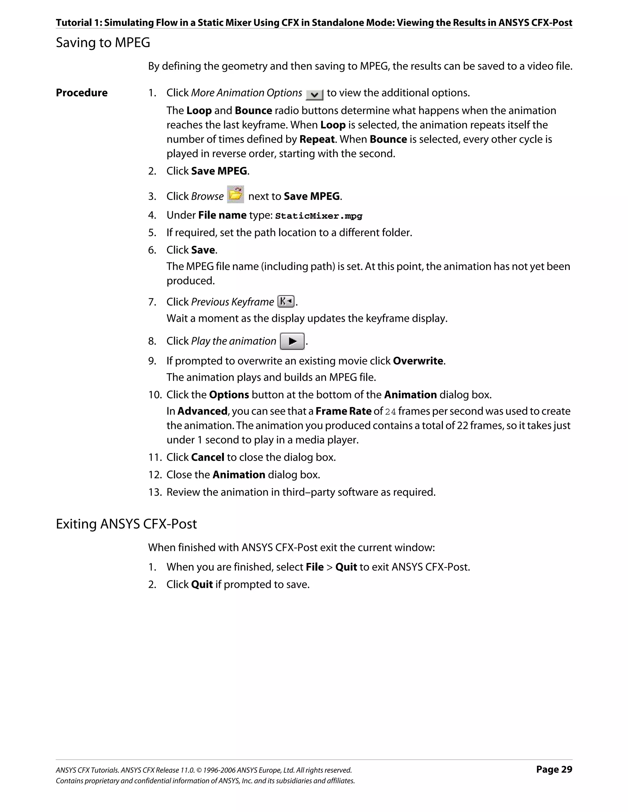

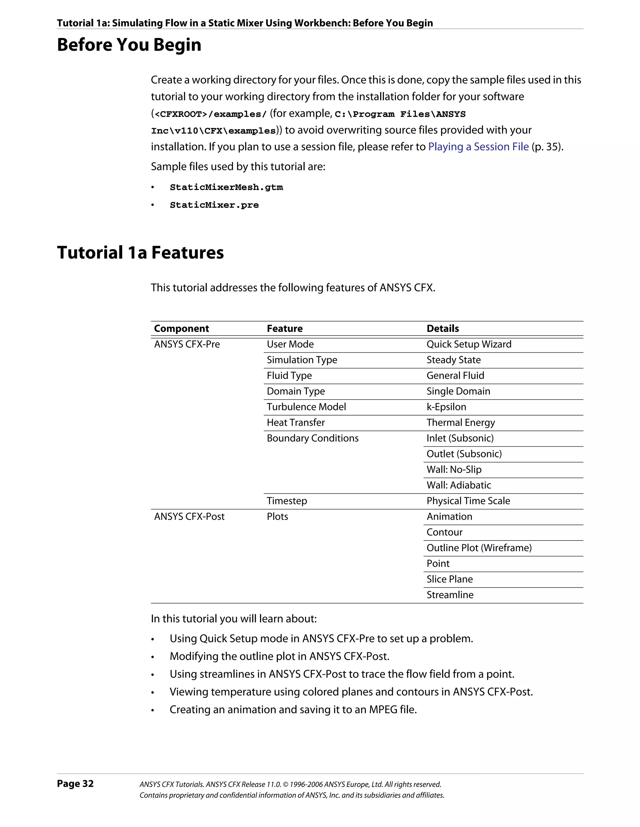
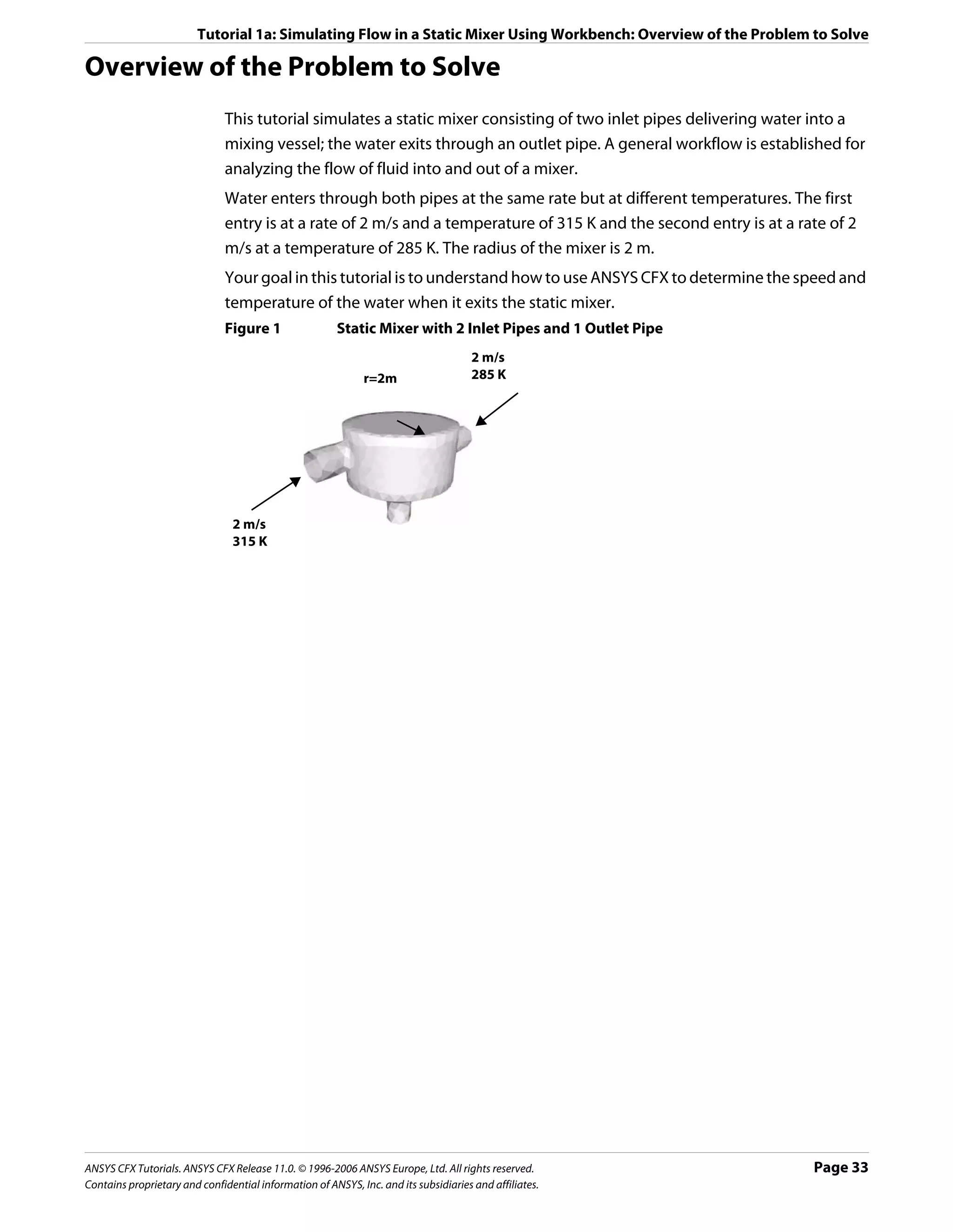
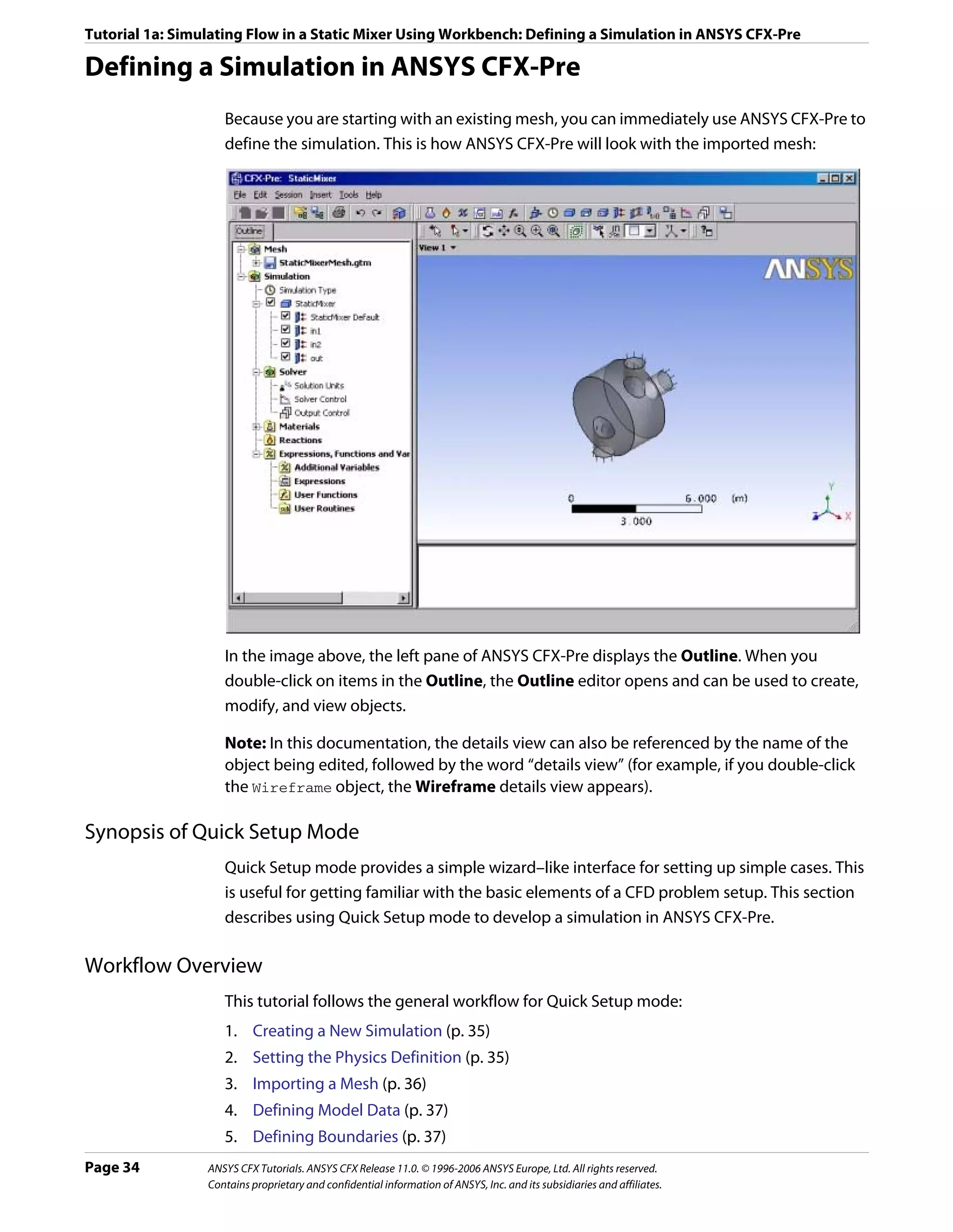
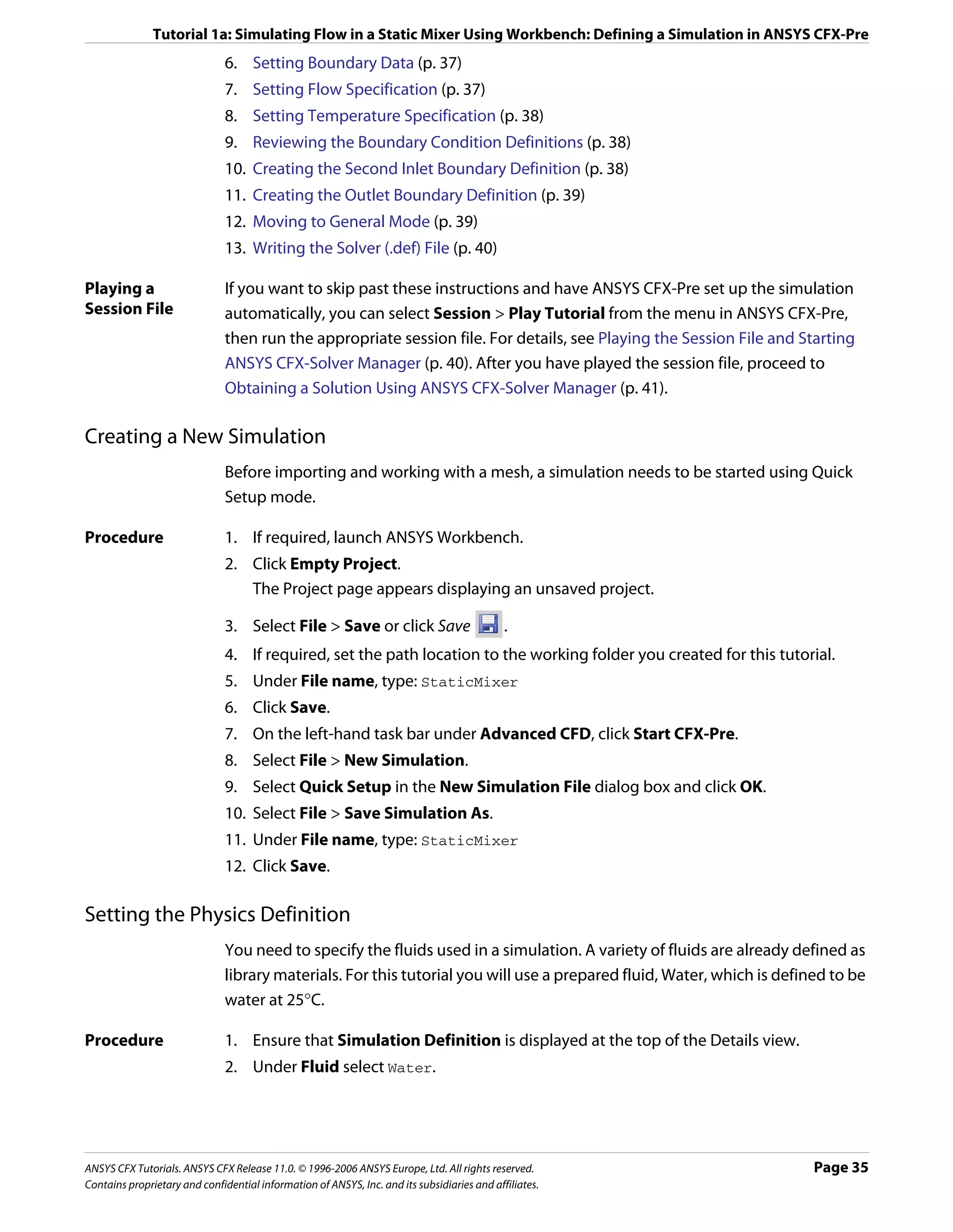
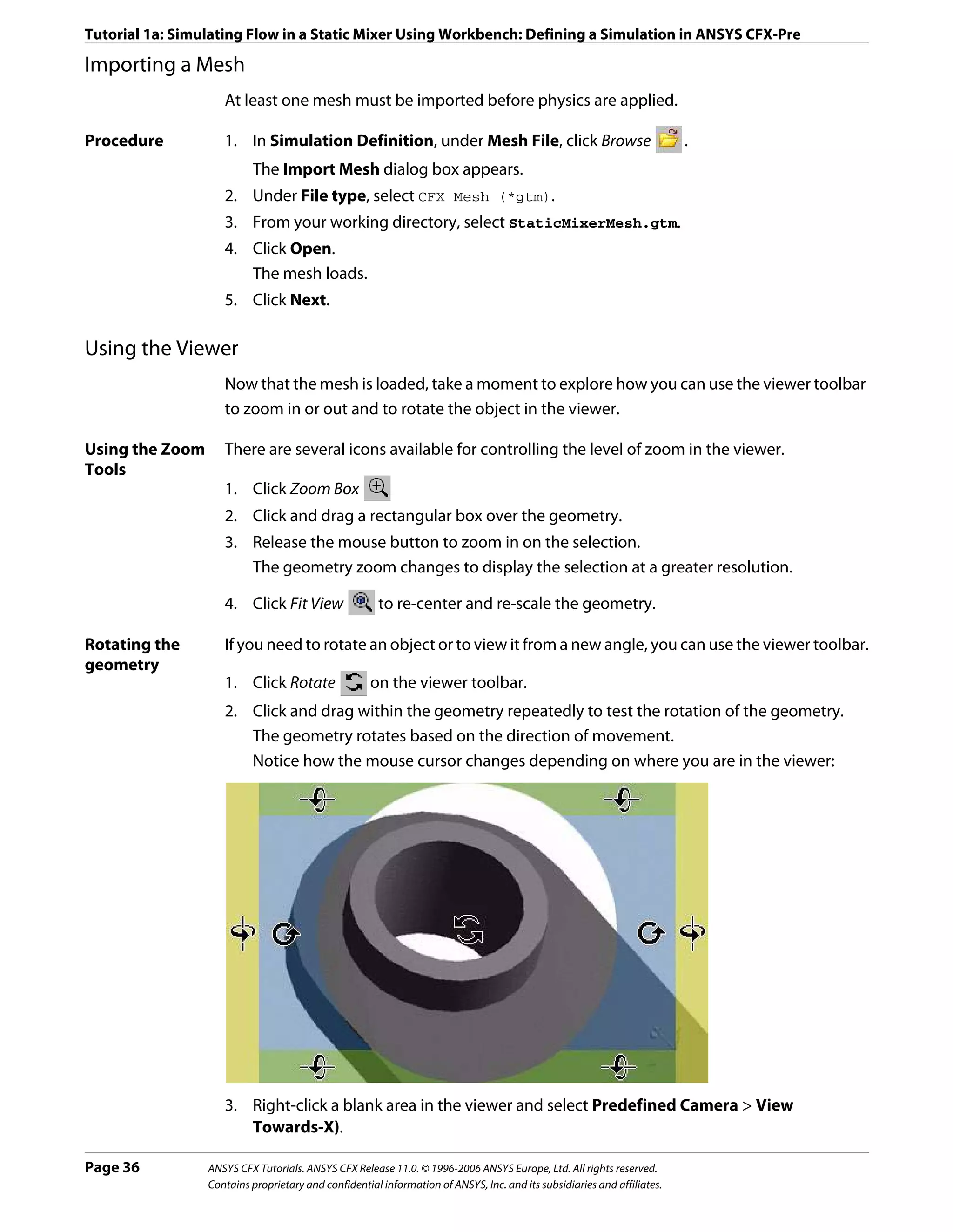
![Tutorial 1a: Simulating Flow in a Static Mixer Using Workbench: Defining a Simulation in ANSYS CFX-Pre
4. Right-click a blank area in the viewer and select Predefined Camera > Isometric View
(Z Up).
A clearer view of the mesh is displayed.
Defining Model Data
You need to define the type of flow and the physical models to use in the fluid domain.
You will specify the flow as steady state with turbulence and heat transfer. Turbulence is
modelled using the k - ε turbulence model and heat transfer using the thermal energy
model. The k - ε turbulence model is a commonly used model and is suitable for a wide
range of applications. The thermal energy model neglects high speed energy effects and is
therefore suitable for low speed flow applications.
Procedure 1. Ensure that Physics Definition is displayed.
2. Under Model Data, set Reference Pressure to 1 [atm].
All other pressure settings are relative to this reference pressure.
3. Set Heat Transfer to Thermal Energy.
4. Set Turbulence to k-Epsilon.
5. Click Next.
Defining Boundaries
The CFD model requires the definition of conditions on the boundaries of the domain.
Procedure 1. Ensure that Boundary Definition is displayed.
2. Delete Inlet and Outlet from the list by right-clicking each and selecting Delete.
3. Right-click in the blank area where Inlet and Outlet were listed, then select New.
4. Set Name to: in1
5. Click OK.
The boundary is created and, when selected, properties related to the boundary are
displayed.
Setting Boundary Data
Once boundaries are created, you need to create associated data. Based on Figure 1, you will
define the first inlet boundary condition to have a velocity of 2 m/s and a temperature of 315
K at one of the side inlets.
Procedure 1. Ensure that Boundary Data is displayed.
2. Set Boundary Type to Inlet.
3. Set Location to in1.
Setting Flow Specification
Once boundary data is defined, the boundary needs to have the flow specification assigned.
ANSYS CFX Tutorials. ANSYS CFX Release 11.0. © 1996-2006 ANSYS Europe, Ltd. All rights reserved. Page 37
Contains proprietary and confidential information of ANSYS, Inc. and its subsidiaries and affiliates.](https://image.slidesharecdn.com/ansys11tutorial-111218135319-phpapp01/75/Ansys-11-tutorial-49-2048.jpg)
![Tutorial 1a: Simulating Flow in a Static Mixer Using Workbench: Defining a Simulation in ANSYS CFX-Pre
Procedure 1. Ensure that Flow Specification is displayed.
2. Set Option to Normal Speed.
3. Set Normal Speed to 2 [m s^-1].
Setting Temperature Specification
Once flow specification is defined, the boundary needs to have temperature assigned.
Procedure 1. Ensure that Temperature Specification is displayed.
2. Set Static Temperature to 315 [K].
Reviewing the Boundary Condition Definitions
Defining the boundary condition for in1 required several steps. Here the settings are
reviewed for accuracy.
Based on Figure 1, the first inlet boundary condition consists of a velocity of 2 m/s and a
temperature of 315 K at one of the side inlets.
Procedure 1. Review the boundary in1 settings for accuracy. They should be as follows:
Tab Setting Value
Boundary Data Boundary Type Inlet
Location in1
Flow Specification Option Normal Speed
Normal Speed 2 [m s^-1]
Temperature Specification Static Temperature 315 [K]
Creating the Second Inlet Boundary Definition
Based on Figure 1, you know the second inlet boundary condition consists of a velocity of 2
m/s and a temperature of 285 K at one of the side inlets. You will define that now.
Procedure 1. Under Boundary Definition, right-click in the selector area and select New.
2. Create a new boundary named in2 with these settings:
Tab Setting Value
Boundary Data Boundary Type Inlet
Location in2
Flow Specification Option Normal Speed
Normal Speed 2 [m s^-1]
Temperature Specification Static Temperature 285 [K]
Page 38 ANSYS CFX Tutorials. ANSYS CFX Release 11.0. © 1996-2006 ANSYS Europe, Ltd. All rights reserved.
Contains proprietary and confidential information of ANSYS, Inc. and its subsidiaries and affiliates.](https://image.slidesharecdn.com/ansys11tutorial-111218135319-phpapp01/75/Ansys-11-tutorial-50-2048.jpg)
![Tutorial 1a: Simulating Flow in a Static Mixer Using Workbench: Defining a Simulation in ANSYS CFX-Pre
Creating the Outlet Boundary Definition
Now that the second inlet boundary has been created, the same concepts can be applied to
building the outlet boundary.
1. Create a new boundary named out with these settings:
Tab Setting Value
Boundary Data Boundary Type Outlet
Location out
Flow Specification Option Average Static Pressure
Relative Pressure 0 [Pa]
2. Click Next.
Moving to General Mode
There are no further boundary conditions that need to be set. All 2D exterior regions that
have not been assigned to a boundary condition are automatically assigned to the default
boundary condition.
Procedure 1. Set Operation to Enter General Mode and click Finish.
The three boundary conditions are displayed in the viewer as sets of arrows at the
boundary surfaces. Inlet boundary arrows are directed into the domain. Outlet
boundary arrows are directed out of the domain.
Setting Solver Control
Solver Control parameters control aspects of the numerical solution generation process.
While an upwind advection scheme is less accurate than other advection schemes, it is also
more robust. This advection scheme is suitable for obtaining an initial set of results, but in
general should not be used to obtain final accurate results.
The time scale can be calculated automatically by the solver or set manually. The Automatic
option tends to be conservative, leading to reliable, but often slow, convergence. It is often
possible to accelerate convergence by applying a time scale factor or by choosing a manual
value that is more aggressive than the Automatic option. In this tutorial, you will select a
physical time scale, leading to convergence that is twice as fast as the Automatic option.
Procedure 1. Click Solver Control .
2. On the Basic Settings tab, set Advection Scheme > Option to Upwind.
3. Set Convergence Control > Fluid Timescale Control > Timescale Control to
Physical Timescale and set the physical timescale value to 2 [s].
4. Click OK.
ANSYS CFX Tutorials. ANSYS CFX Release 11.0. © 1996-2006 ANSYS Europe, Ltd. All rights reserved. Page 39
Contains proprietary and confidential information of ANSYS, Inc. and its subsidiaries and affiliates.](https://image.slidesharecdn.com/ansys11tutorial-111218135319-phpapp01/75/Ansys-11-tutorial-51-2048.jpg)
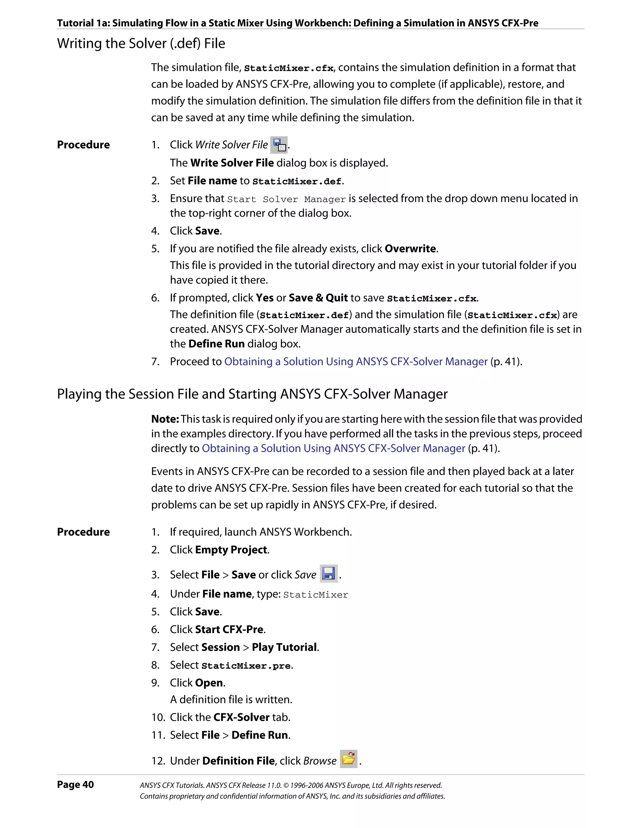
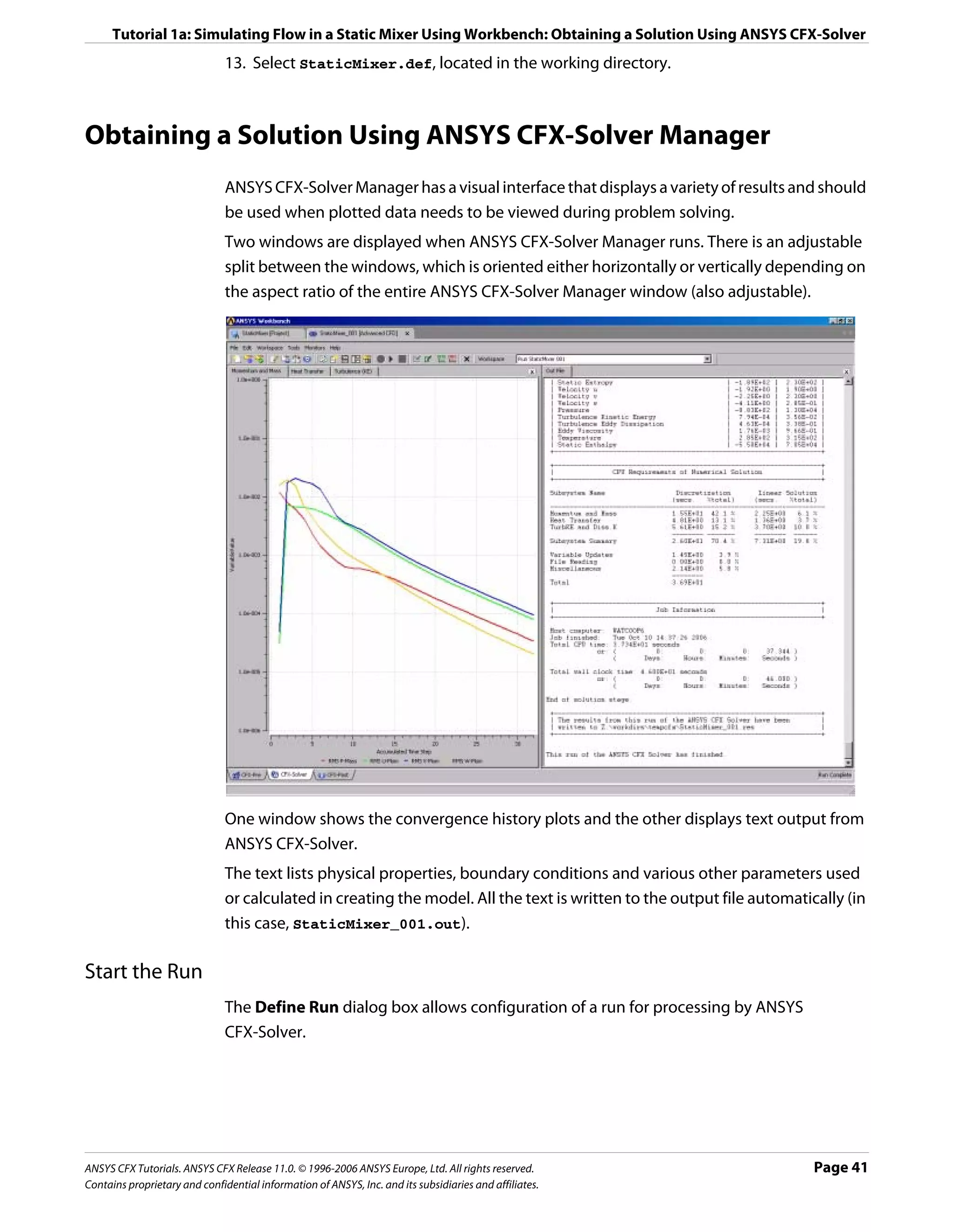
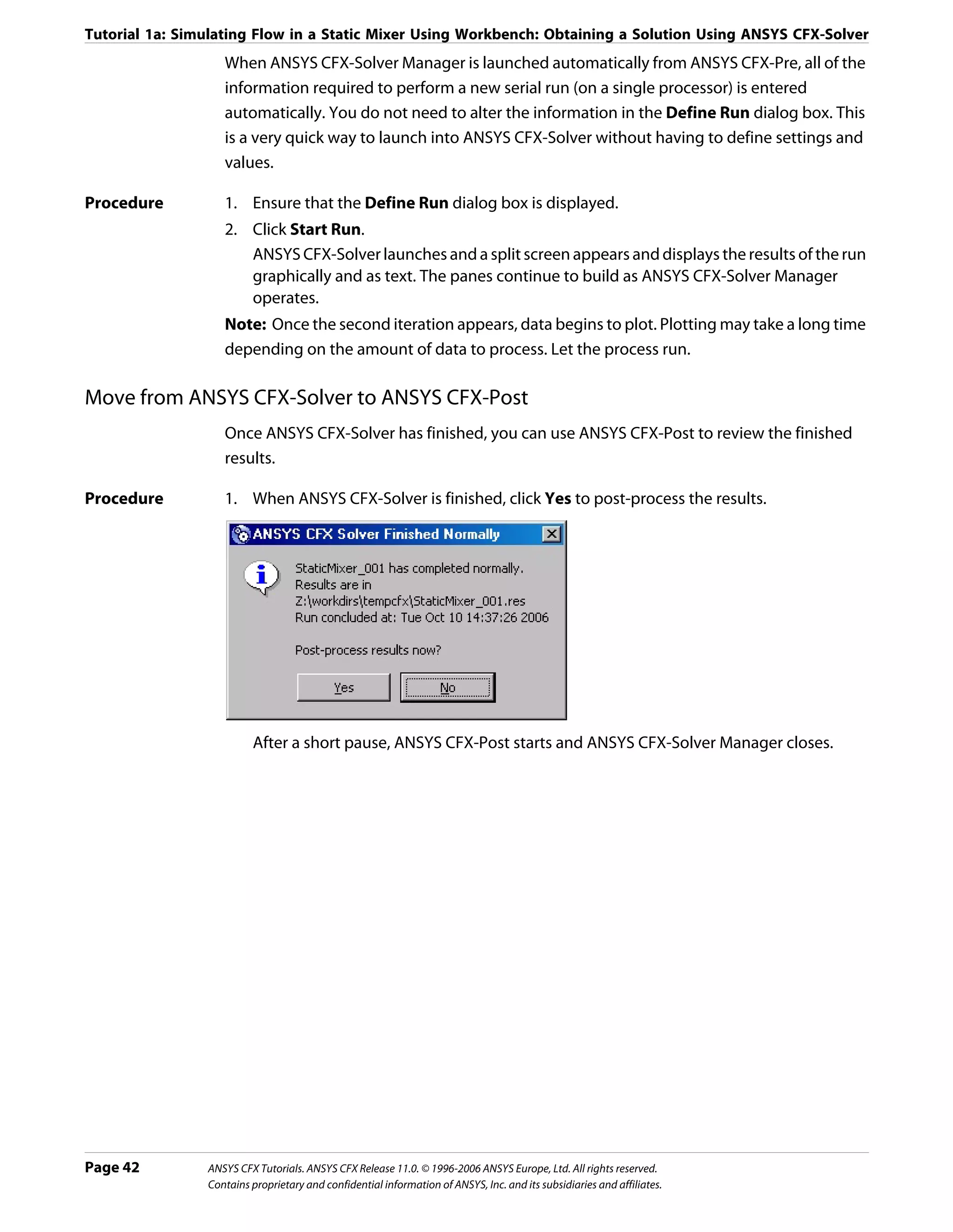
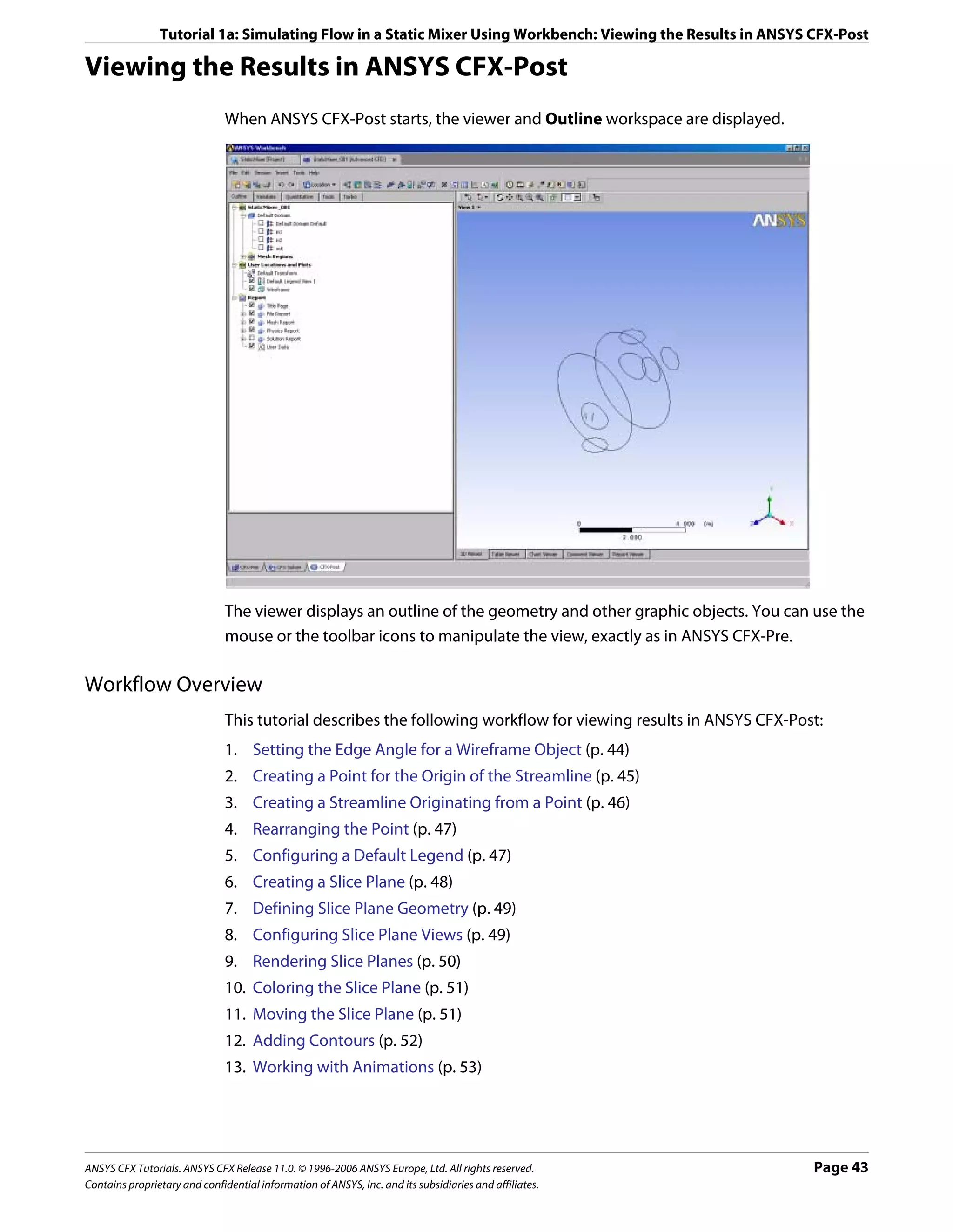
![Tutorial 1a: Simulating Flow in a Static Mixer Using Workbench: Viewing the Results in ANSYS CFX-Post
Setting the Edge Angle for a Wireframe Object
The outline of the geometry is called the wireframe or outline plot.
By default, ANSYS CFX-Post displays only some of the surface mesh. This sometimes means
that when you first load your results file, the geometry outline is not displayed clearly. You
can control the amount of the surface mesh shown by editing the Wireframe object listed
in the Outline.
The check boxes next to each object name in the Outline control the visibility of each
object. Currently only the Wireframe and Default Legend objects have visibility selected.
The edge angle determines how much of the surface mesh is visible. If the angle between
two adjacent faces is greater than the edge angle, then that edge is drawn. If the edge angle
is set to 0°, the entire surface mesh is drawn. If the edge angle is large, then only the most
significant corner edges of the geometry are drawn.
For this geometry, a setting of approximately 15° lets you view the model location without
displaying an excessive amount of the surface mesh.
In this module you can also modify the zoom settings and view of the wireframe.
Procedure 1. In the Outline, under User Locations and Plots, double-click Wireframe.
Tip: While it is not necessary to change the view to set the angle, do so to explore the
practical uses of this feature.
2. Right-click on a blank area anywhere in the viewer, select Predefined Camera from the
shortcut menu and select Isometric View (Z up).
3. In the Wireframe details view, under Definition, click in the Edge Angle box.
An embedded slider is displayed.
4. Type a value of 10 [degree].
5. Click Apply to update the object with the new setting.
Page 44 ANSYS CFX Tutorials. ANSYS CFX Release 11.0. © 1996-2006 ANSYS Europe, Ltd. All rights reserved.
Contains proprietary and confidential information of ANSYS, Inc. and its subsidiaries and affiliates.](https://image.slidesharecdn.com/ansys11tutorial-111218135319-phpapp01/75/Ansys-11-tutorial-56-2048.jpg)
![Tutorial 1a: Simulating Flow in a Static Mixer Using Workbench: Viewing the Results in ANSYS CFX-Post
Notice that more surface mesh is displayed.
6. Drag the embedded slider to set the Edge Angle value to approximately 45 [degree].
7. Click Apply to update the object with the new setting.
Less of the outline of the geometry is displayed.
8. Type a value of 15 [degree].
9. Click Apply to update the object with the new setting.
10. Right-click on a blank area anywhere in the viewer, select Predefined Camera from the
shortcut menu and select View Towards -X.
Creating a Point for the Origin of the Streamline
A streamline is the path that a particle of zero mass would follow through the domain.
Procedure 1. Select Insert > Location > Point from the main menu.
You can also use the toolbars to create a variety of objects. Later modules and tutorials
explore this further.
2. Click OK.
This accepts the default name.
3. Under Definition, ensure that Method is set to XYZ.
4. Under Point, enter the following coordinates: -1, -1, 1.
This is a point near the first inlet.
5. Click Apply.
The point appears as a symbol in the viewer as a crosshair symbol.
ANSYS CFX Tutorials. ANSYS CFX Release 11.0. © 1996-2006 ANSYS Europe, Ltd. All rights reserved. Page 45
Contains proprietary and confidential information of ANSYS, Inc. and its subsidiaries and affiliates.](https://image.slidesharecdn.com/ansys11tutorial-111218135319-phpapp01/75/Ansys-11-tutorial-57-2048.jpg)
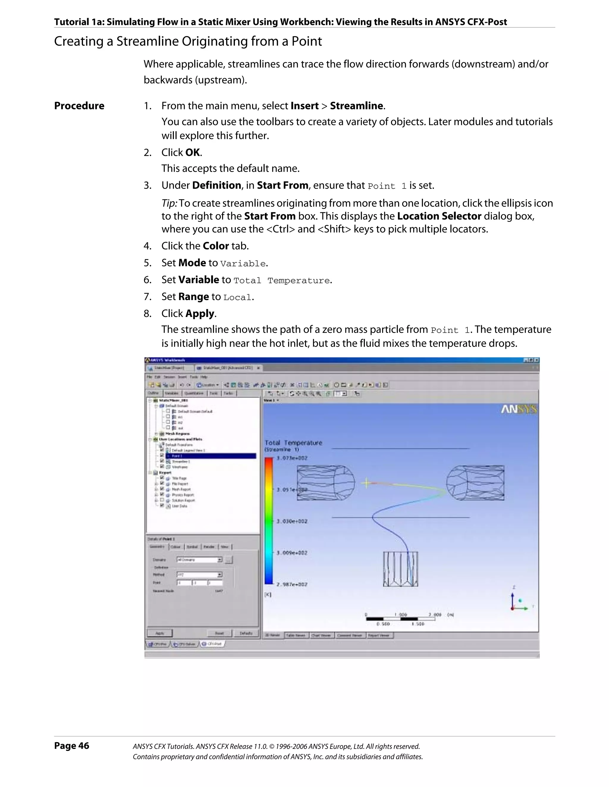
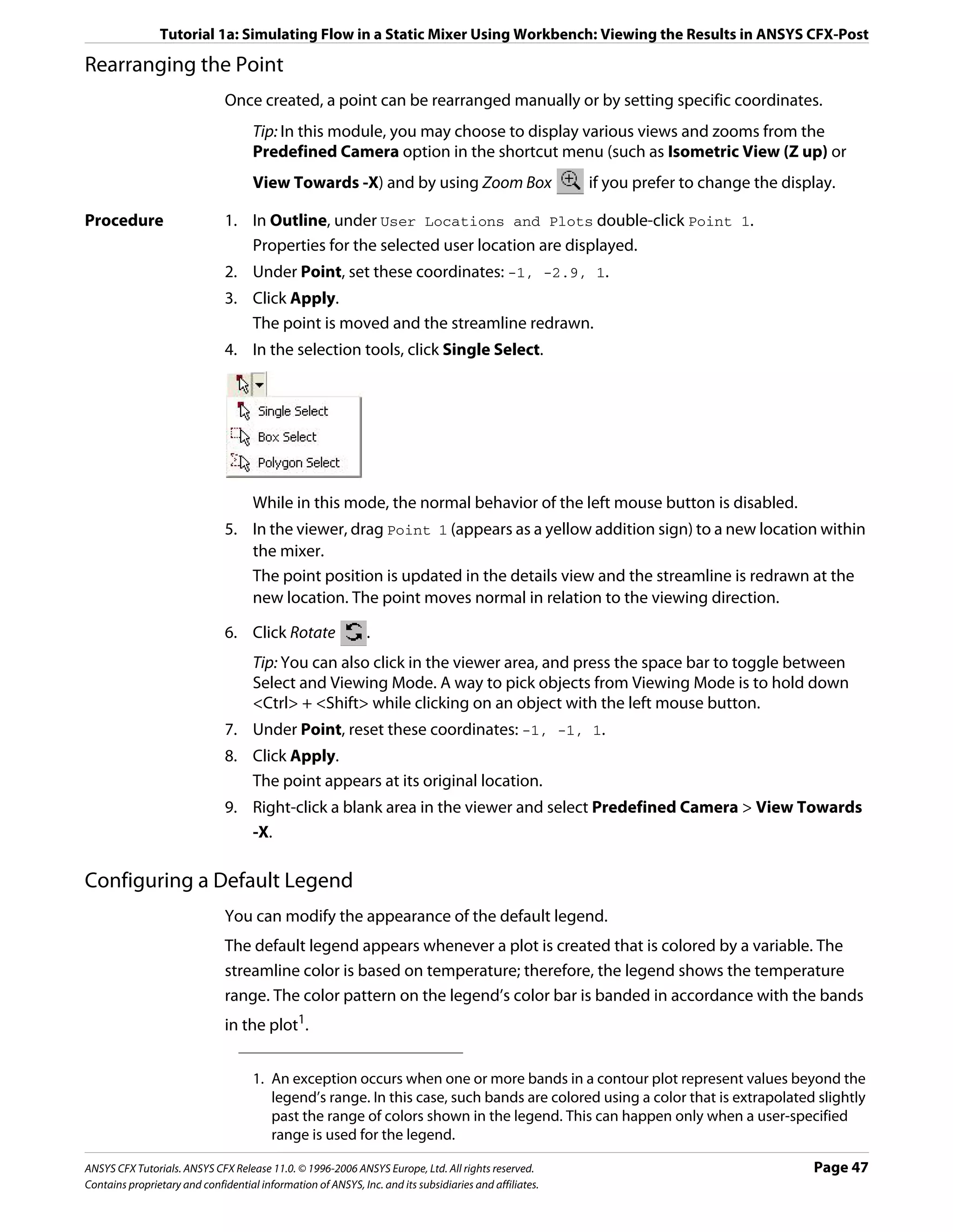
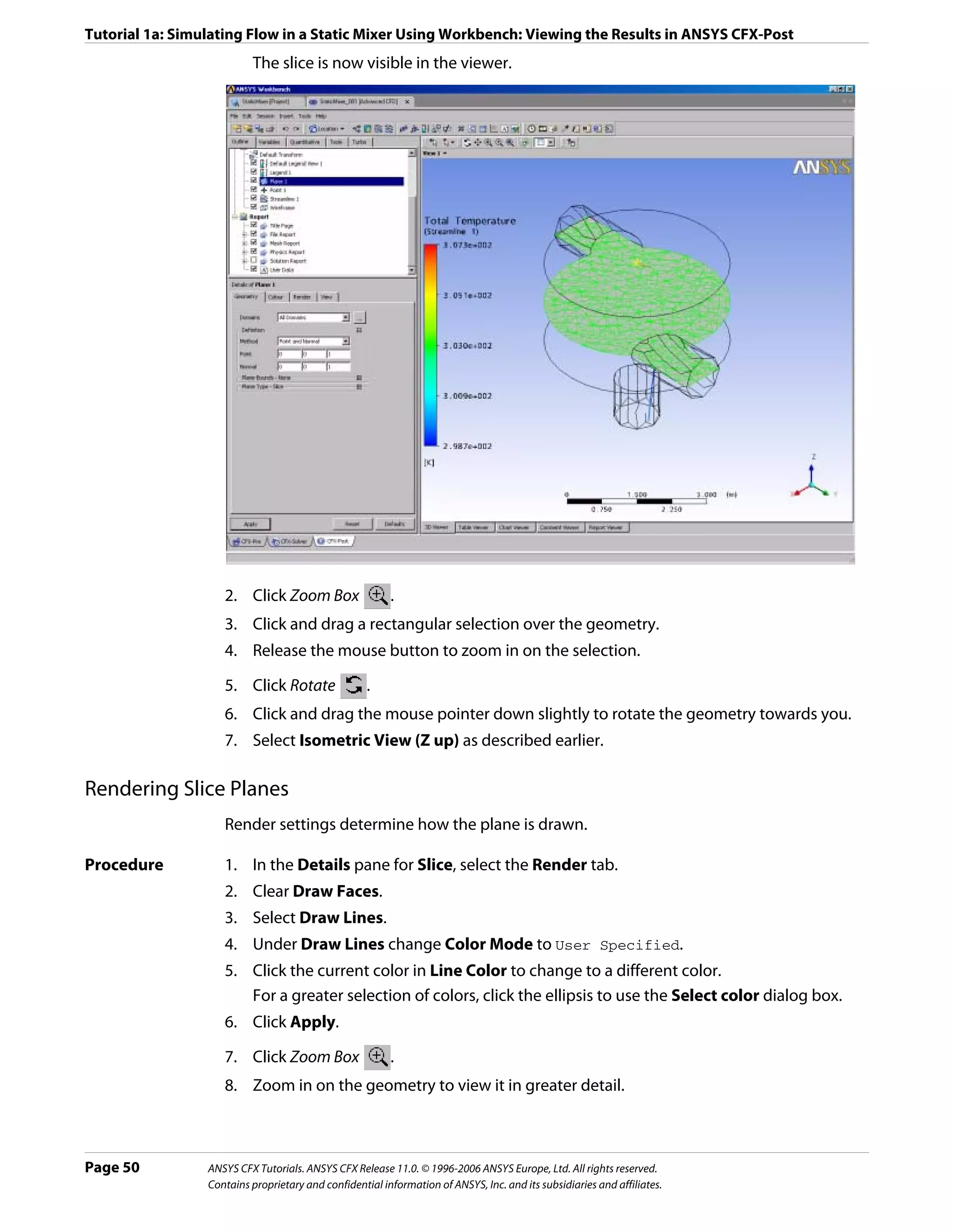


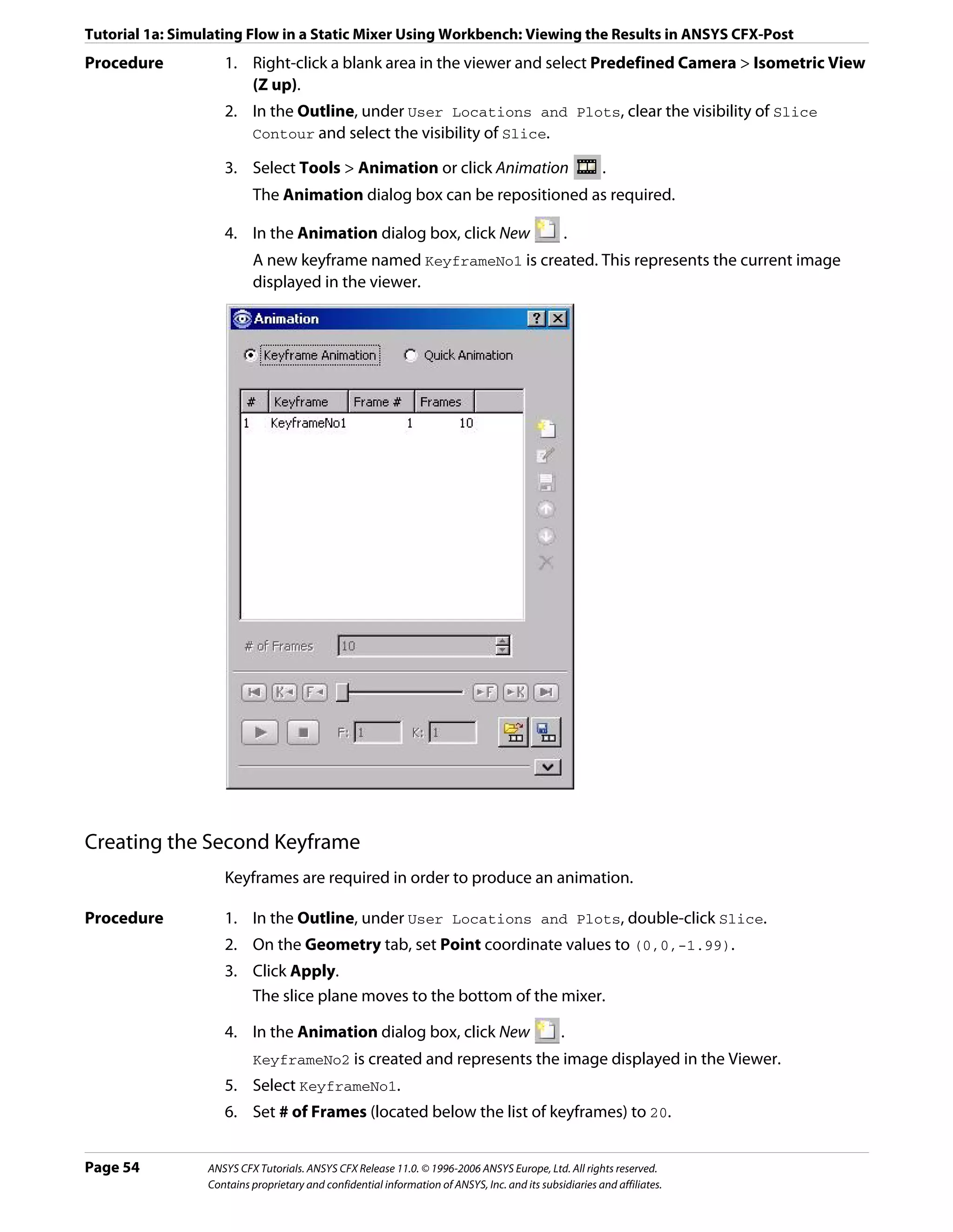
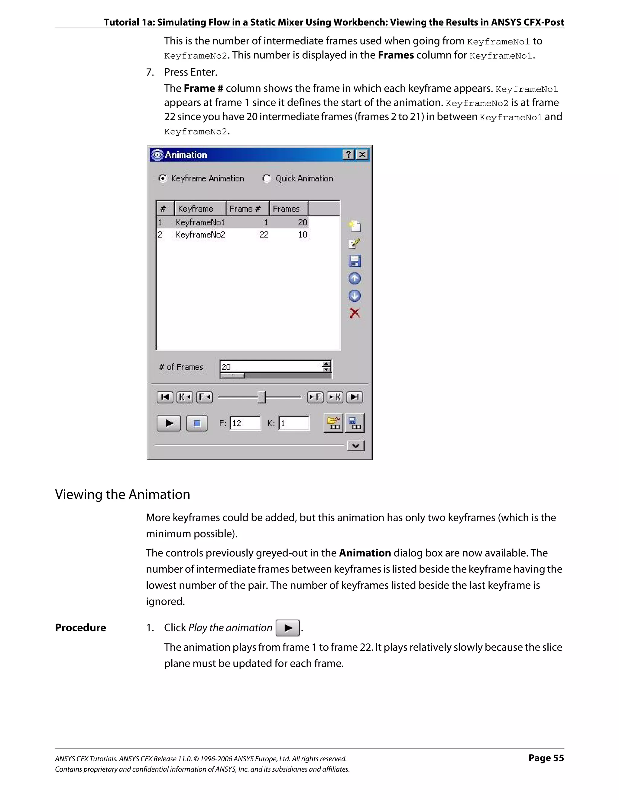
![Tutorial 1a: Simulating Flow in a Static Mixer Using Workbench: Viewing the Results in ANSYS CFX-Post
Modifying the Animation
To make the plane sweep through the whole geometry, you will set the starting position of
the plane to be at the top of the mixer. You will also modify the Range properties of the
plane so that it shows the temperature variation better. As the animation is played, you can
see the hot and cold water entering the mixer. Near the bottom of the mixer (where the
water flows out) you can see that the temperature is quite uniform. The new temperature
range lets you view the mixing process more accurately than the global range used in the
first animation.
Procedure 1. Apply the following settings to Slice
Tab Setting Value
Geometry Point 0, 0, 1.99
Color Mode Variable
Range User Specified
Min 295 [K]
Max 305 [K]
2. Click Apply.
The slice plane moves to the top of the static mixer.
Note: Do not double click in the next step.
3. In the Animation dialog box, single click (do not double-click) KeyframeNo1 to select it.
If you had double-clicked KeyFrameNo1, the plane and viewer states would have been
redefined according to the stored settings for KeyFrameNo1. If this happens, click
Undo and try again to select the keyframe.
4. Click Set Keyframe .
The image in the Viewer replaces the one previously associated with KeyframeNo1.
5. Double-click KeyframeNo2.
The object properties for the slice plane are updated according to the settings in
KeyFrameNo2.
6. Apply the following settings to Slice
Tab Setting Value
Color Mode Variable
Range User Specified
Min 295 [K]
Max 305 [K]
7. Click Apply.
8. In the Animation dialog box, single-click KeyframeNo2.
9. Click Set Keyframe to save the new settings to KeyframeNo2.
Page 56 ANSYS CFX Tutorials. ANSYS CFX Release 11.0. © 1996-2006 ANSYS Europe, Ltd. All rights reserved.
Contains proprietary and confidential information of ANSYS, Inc. and its subsidiaries and affiliates.](https://image.slidesharecdn.com/ansys11tutorial-111218135319-phpapp01/75/Ansys-11-tutorial-68-2048.jpg)


![Tutorial 2: Flow in a Static Mixer (Refined Mesh): Defining a Simulation using General Mode in ANSYS CFX-Pre
Viewing the Boundary Condition Setting
For the k-epsilon turbulence model, you must specify the turbulent nature of the flow
entering through the inlet boundary. For this simulation, the default setting of Medium
(Intensity = 5%) is used. This is a sensible setting if you do not know the turbulence
properties of the incoming flow.
Procedure 1. Under Default Domain, double-click in1.
2. Click the Boundary Details tab and review the settings for Flow Regime, Mass and
Momentum, Turbulence and Heat Transfer.
3. Click Close.
Defining Solver Parameters
Solver Control parameters control aspects of the numerical-solution generation process.
In Tutorial 1 you set some solver control parameters, such as Advection Scheme and
Timescale Control, while other parameters were set automatically by ANSYS CFX-Pre.
In this tutorial, High Resolution is used for the advection scheme. This is more accurate
than the Upwind Scheme used in Tutorial 1. You usually require a smaller timestep when
using this model. You can also expect the solution to take a higher number of iterations to
converge when using this model.
Procedure 1. Select Insert > Solver > Solver Control from the main menu or click Solver Control .
2. Apply the following Basic Settings
Setting Value
Advection Scheme > Option High Resolution
Convergence Control > Max. Iterations* 150
Convergence Control > Fluid Timescale Control > Physical Timescale
Timescale Control
Convergence Control > Fluid Timescale Control > Physical 0.5 [s]
Timescale
*. If your solution does not meet the convergence criteria after this number of
timesteps, the ANSYS CFX-Solver will stop.
3. Click Apply.
4. Click the Advanced Options tab.
5. Ensure that Global Dynamic Model Control is selected.
6. Click OK.
Writing the Solver (.def) File
Once all boundaries are created you move from ANSYS CFX-Pre into ANSYS CFX-Solver.
Page 64 ANSYS CFX Tutorials. ANSYS CFX Release 11.0. © 1996-2006 ANSYS Europe, Ltd. All rights reserved.
Contains proprietary and confidential information of ANSYS, Inc. and its subsidiaries and affiliates.](https://image.slidesharecdn.com/ansys11tutorial-111218135319-phpapp01/75/Ansys-11-tutorial-76-2048.jpg)
![Tutorial 2: Flow in a Static Mixer (Refined Mesh): Viewing the Results in ANSYS CFX-Post
After a short pause, ANSYS CFX-Post starts.
Viewing the Results in ANSYS CFX-Post
In the following sections, you will explore the differences between the mesh and the results
from this tutorial and tutorial 1.
Creating a Slice Plane
More information exists for use by ANSYS CFX-Post in this tutorial than in Tutorial 1 because
the slice plane is more detailed.
Once a new slice plane is created it can be compared with Tutorial 1. There are three
noticeable differences between the two slice planes.
• Around the edges of the mixer geometry there are several layers of narrow rectangles.
This is the region where the mesh contains prismatic elements (which are created as
inflation layers). The bulk of the geometry contains tetrahedral elements.
• There are more lines on the plane than there were in Tutorial 1. This is because the slice
plane intersects with more mesh elements.
• The curves of the mixer are smoother than in Tutorial 1 because the finer mesh better
represents the true geometry.
Procedure 1. Right-click a blank area in the viewer and select Predefined Camera > Isometric View
(Z up).
2. From the main menu, select Insert > Location > Plane or under Location, click Plane.
3. In the Insert Plane dialog box, type Slice and click OK.
The Geometry, Color, Render and View tabs let you switch between settings.
4. Apply the following settings
Tab Setting Value
Geometry Domains Default Domain
Definition > Method XY Plane
Definition > Z 1 [m]
Render Draw Faces (Cleared)
Draw Lines (Selected)
5. Click Apply.
6. Right-click a blank area in the viewer and select Predefined Camera > View Towards
-Z.
7. Click Zoom Box .
8. Zoom in on the geometry to view it in greater detail.
Page 68 ANSYS CFX Tutorials. ANSYS CFX Release 11.0. © 1996-2006 ANSYS Europe, Ltd. All rights reserved.
Contains proprietary and confidential information of ANSYS, Inc. and its subsidiaries and affiliates.](https://image.slidesharecdn.com/ansys11tutorial-111218135319-phpapp01/75/Ansys-11-tutorial-80-2048.jpg)
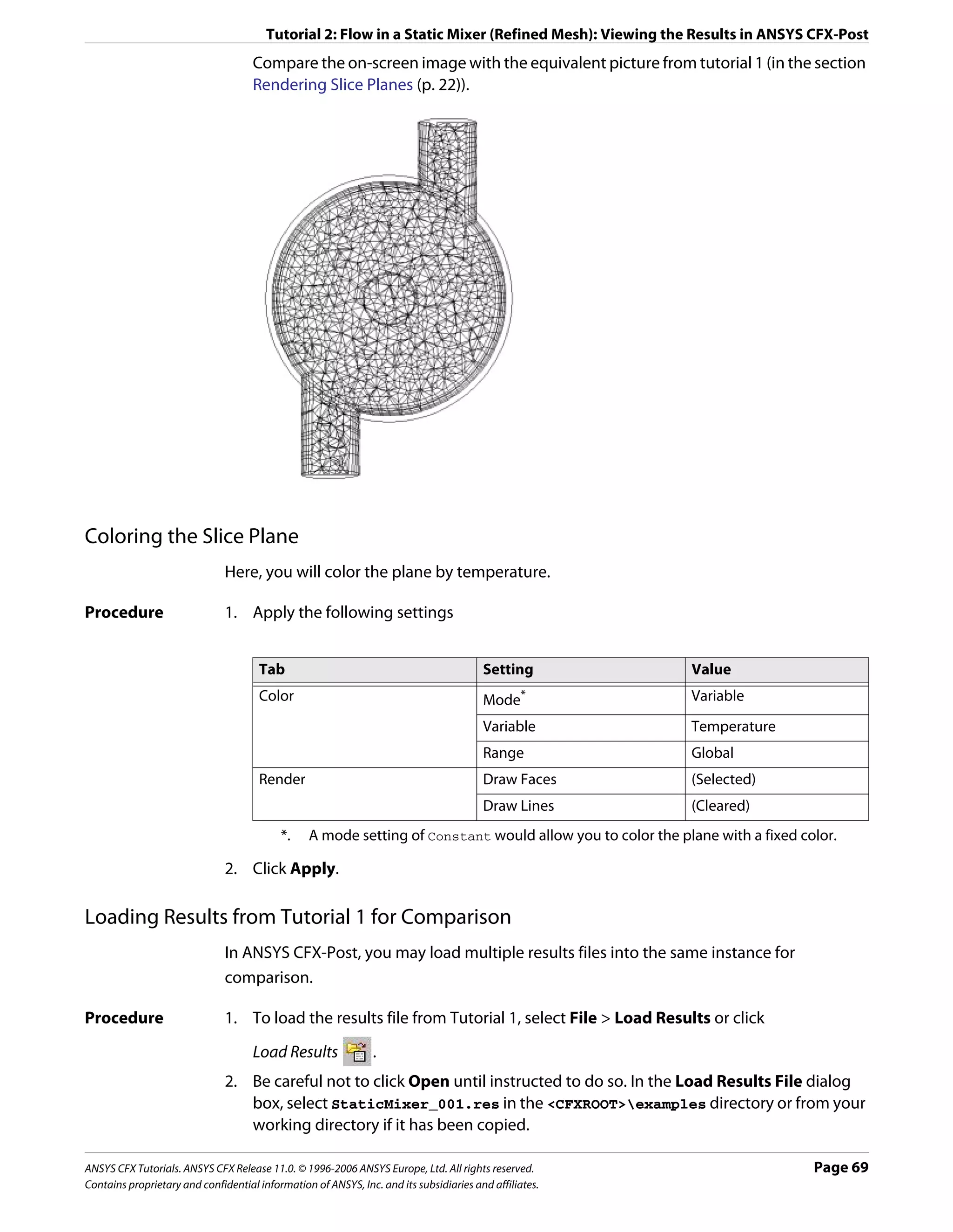
![Tutorial 2: Flow in a Static Mixer (Refined Mesh): Viewing the Results in ANSYS CFX-Post
3. On the right side of the dialog box, there are two frames. Under Results file option,
select Add to current results.
4. Select the Offset in Y direction check box.
5. Under Additional actions, ensure that the Clear user state before loading check box
is cleared.
6. Click Open to load the results.
In the tree view, there is now a second group of domains, meshes and boundary
conditions with the heading StaticMixer_001.
7. Double-click the Wireframe object under User Locations and Plots.
8. In the Definition tab, set Edge Angle to 5 [degree].
9. Click Apply.
10. Right-click a blank area in the viewer and select Predefined Camera > Isometric View
(Z up).
Both meshes are now displayed in a line along the Y axis. Notice that one mesh is of a
higher resolution than the other.
11. Set Edge Angle to 30 [degree].
12. Click Apply.
Creating a Second Slice Plane
Procedure 1. In the tree view, right-click the plane named Slice and select Duplicate.
2. Click OK to accept the default name Slice 1.
3. In the tree view, double-click the plane named Slice 1.
4. On the Geometry tab, set Domains to Default Domain 1.
5. On the Color tab, ensure that Range is set to Global.
6. Click Apply.
7. Double-click Slice and make sure that Range is set to Global.
Comparing Slice Planes using Multiple Views
Procedure 1. Select the option with the two vertical rectangles. Notice that the Viewer now has two
separate views.
The visibility status of each object is maintained separately for each view or figure that
can be displayed in a given viewport. This allows some planes to be shown while others
are hidden.
Page 70 ANSYS CFX Tutorials. ANSYS CFX Release 11.0. © 1996-2006 ANSYS Europe, Ltd. All rights reserved.
Contains proprietary and confidential information of ANSYS, Inc. and its subsidiaries and affiliates.](https://image.slidesharecdn.com/ansys11tutorial-111218135319-phpapp01/75/Ansys-11-tutorial-82-2048.jpg)
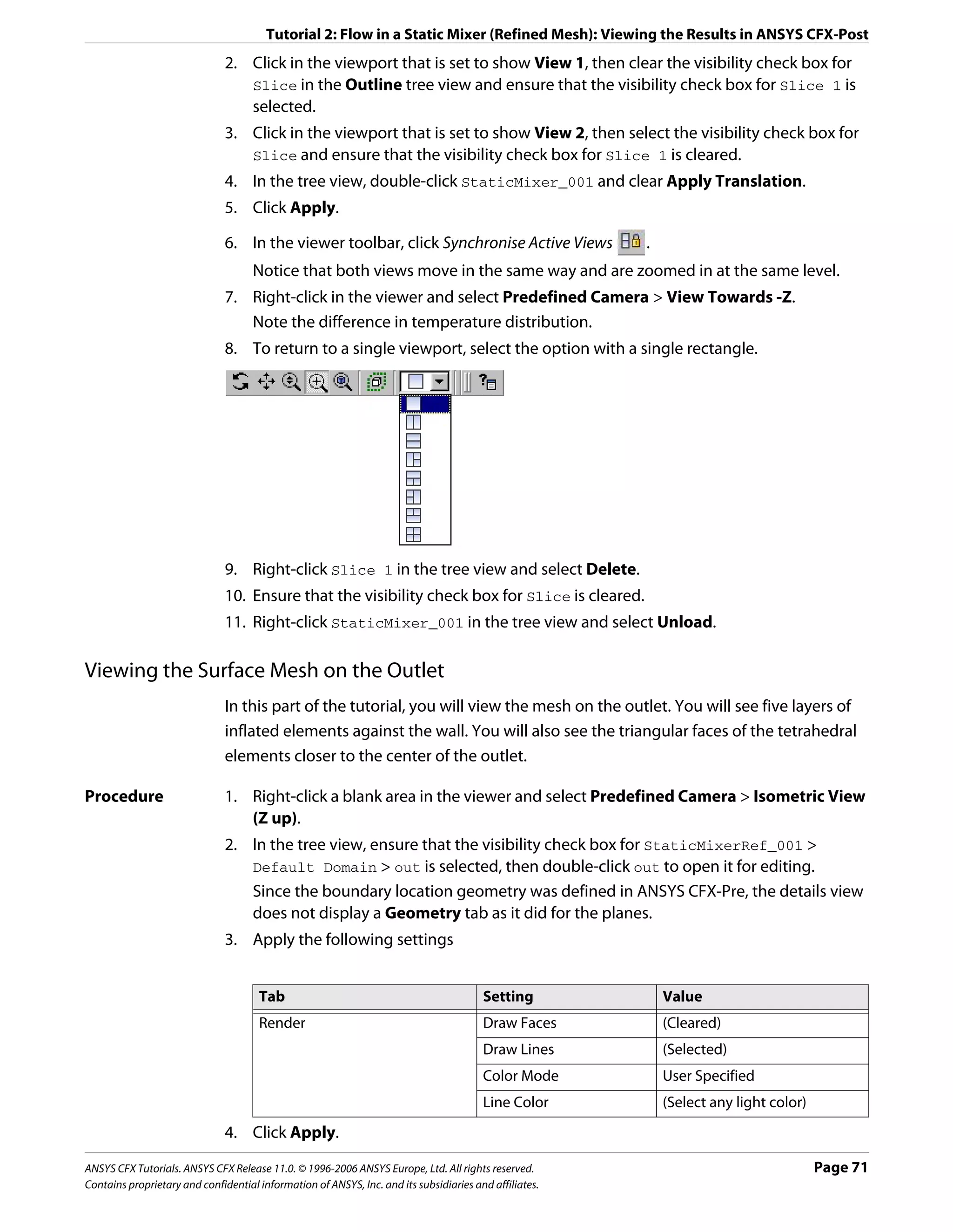
![Tutorial 2: Flow in a Static Mixer (Refined Mesh): Viewing the Results in ANSYS CFX-Post
5. Click Zoom Box .
6. Zoom in on the geometry to view out in greater detail.
7. Click Rotate on the Viewing Tools toolbar.
8. Rotate the image as required to clearly see the mesh.
Looking at the Inflated Elements in Three Dimensions
To show more clearly what effect inflation has on the shape of the elements, you will use
volume objects to show two individual elements. The first element that will be shown is a
normal tetrahedral element; the second is a prismatic element from an inflation layer of the
mesh.
Leave the surface mesh on the outlet visible to help see how surface and volume meshes are
related.
Procedure 1. From the main menu, select Insert > Location > Volume or, under Location click
Volume.
2. In the Insert Volume dialog box, type Tet Volume and click OK.
3. Apply the following settings
Tab Setting Value
Geometry Definition > Method Sphere
Definition > Point * 0.08, 0, -2
Definition > Radius 0.14 [m]
Definition > Mode Below Intersection
Inclusive† (Cleared)
Color Color Red
Render Draw Faces > Transparency 0.3
Draw Lines (Selected)
Draw Lines > Line Width 1
Draw Lines > Color Mode User Specified
Draw Lines > Line Color Grey
*. The z slider’s minimum value corresponds to the minimum z value of the entire
geometry, which, in this case, occurs at the outlet.
†. Only elements that are entirely contained within the sphere volume will be
included.
4. Click Apply to create the volume object.
5. Right-click Tet Volume and choose Duplicate.
6. In the Duplicate Tet Volume dialog box, type Prism Volume and click OK.
7. Double-click Prism Volume.
8. Apply the following settings
Page 72 ANSYS CFX Tutorials. ANSYS CFX Release 11.0. © 1996-2006 ANSYS Europe, Ltd. All rights reserved.
Contains proprietary and confidential information of ANSYS, Inc. and its subsidiaries and affiliates.](https://image.slidesharecdn.com/ansys11tutorial-111218135319-phpapp01/75/Ansys-11-tutorial-84-2048.jpg)
![Tutorial 2: Flow in a Static Mixer (Refined Mesh): Viewing the Results in ANSYS CFX-Post
Tab Setting Value
Geometry Definition > Point -0.22, 0.4, -1.85
Definition > Radius 0.206 [m]
Color Color Orange
9. Click Apply.
Viewing the Surface Mesh on the Mixer Body
Procedure 1. Double-click the Default Domain Default object.
2. Apply the following settings
Tab Setting Value
Render Draw Faces (Selected)
Draw Lines (Selected)
Line Width 2
3. Click Apply.
Viewing the Layers of Inflated Elements on a Plane
You will see the layers of inflated elements on the wall of the main body of the mixer. Within
the body of the mixer, there will be many lines that are drawn wherever the face of a mesh
element intersects the slice plane.
Procedure 1. From the main menu, select Insert > Location > Plane or under Location, click Plane.
2. In the Insert Plane dialog box, type Slice 2 and click OK.
3. Apply the following settings
Tab Setting Value
Geometry Definition > Method YZ Plane
Definition > X 0 [m]
Render Draw Faces (Cleared)
Draw Lines (Selected)
4. Click Apply.
5. Turn off the visibility of all objects except Slice 2.
6. To see the plane clearly, right-click in the viewer and select Predefined Camera > View
Towards -X.
Viewing the Mesh Statistics
You can use the Report Viewer to check the quality of your mesh. For example, you can load
a .def file into ANSYS CFX-Post and check the mesh quality before running the .def file in
the solver.
ANSYS CFX Tutorials. ANSYS CFX Release 11.0. © 1996-2006 ANSYS Europe, Ltd. All rights reserved. Page 73
Contains proprietary and confidential information of ANSYS, Inc. and its subsidiaries and affiliates.](https://image.slidesharecdn.com/ansys11tutorial-111218135319-phpapp01/75/Ansys-11-tutorial-85-2048.jpg)
![Tutorial 2: Flow in a Static Mixer (Refined Mesh): Viewing the Results in ANSYS CFX-Post
Procedure 1. Click the Report Viewer tab (located below the viewer window).
A report appears. Look at the table shown in the “Mesh Report” section.
2. Double-click Report > Mesh Report in the Outline tree view.
3. In the Mesh Report details view, select Statistics > Maximum Face Angle.
4. Click Refresh Preview.
Note that a new table, showing the maximum face angle for all elements in the mesh,
has been added to the “Mesh Report” section of the report. The maximum face angle is
reported as 148.95°.
As a result of generating this mesh statistic for the report, a new variable, Maximum Face
Angle, has been created and stored at every node. This variable will be used in the next
section.
Viewing the Mesh Elements with Largest Face Angle
In this section, you will visualize the mesh elements that have a Maximum Face Angle value
greater than 140°.
Procedure 1. Click the 3D Viewer tab (located below the viewer window).
2. Right-click a blank area in the viewer and select Predefined Camera > Isometric View
(Z up).
3. In the Outline tree view, select the visibility check box of Wireframe.
4. From the main menu, select Insert > Location > Volume or under Location, click
Volume.
5. In the Insert Volume dialog box, type Max Face Angle Volume and click OK.
6. Apply the following settings
Tab Setting Value
Geometry Definition > Method Isovolume
Definition > Variable Maximum Face Angle*
Definition > Mode Above Value
Definition > Value 140 [degree]
Inclusive† (Selected)
*. Select Maximum Face Angle from the larger list of variables available by clicking
to the right of the Variable box.
†. This includes any elements that have at least one node with a variable value greater
than or equal to the given value.
7. Click Apply.
The volume object appears in the viewer.
Page 74 ANSYS CFX Tutorials. ANSYS CFX Release 11.0. © 1996-2006 ANSYS Europe, Ltd. All rights reserved.
Contains proprietary and confidential information of ANSYS, Inc. and its subsidiaries and affiliates.](https://image.slidesharecdn.com/ansys11tutorial-111218135319-phpapp01/75/Ansys-11-tutorial-86-2048.jpg)


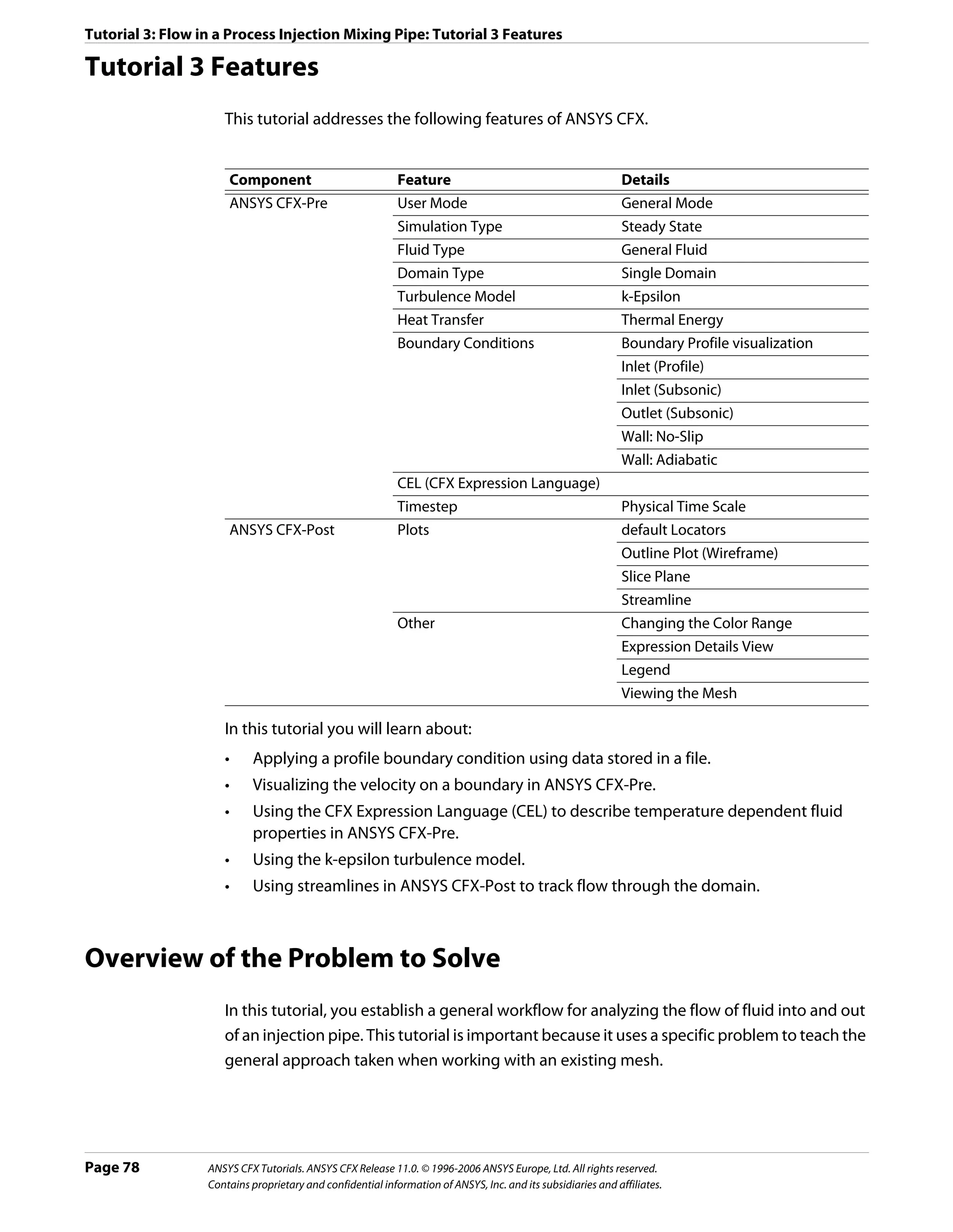
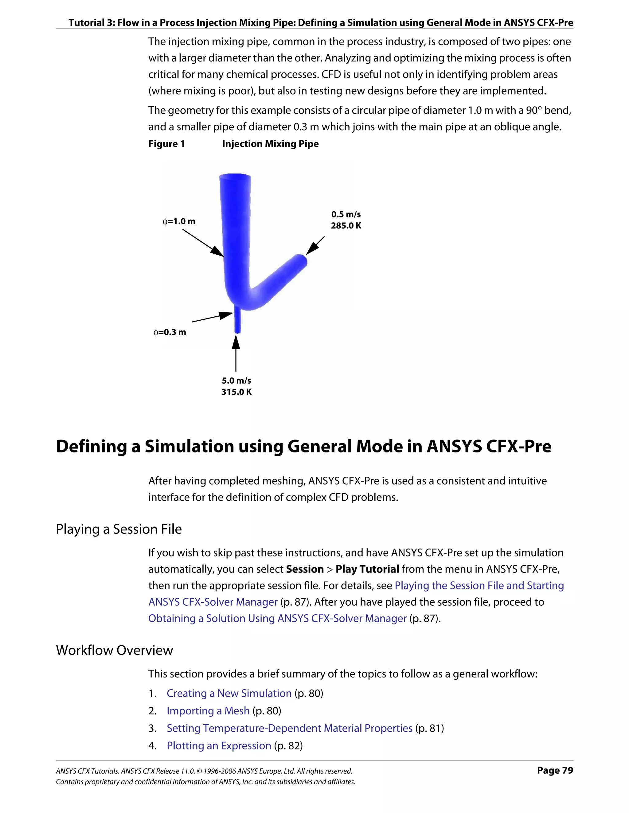

![Tutorial 3: Flow in a Process Injection Mixing Pipe: Defining a Simulation using General Mode in ANSYS CFX-Pre
Procedure 1. Select File > Import Mesh.
2. From your tutorial directory, select InjectMixerMesh.gtm.
3. Click Open.
4. Right-click a blank area in the viewer and select Predefined Camera > Isometric View
(Y up) from the shortcut menu.
Setting Temperature-Dependent Material Properties
You will create an expression for viscosity as a function of temperature and then use this
expression to modify the properties of the library material: Water.
Viscosity will be made to vary linearly with temperature between the following conditions:
• µ =1.8E-03 N s m-2 at T=275.0 K
• µ =5.45E-04 N s m-2 at T=325.0 K
The variable T (Temperature) is a ANSYS CFX System Variable recognized by ANSYS CFX-Pre,
denoting static temperature. All variables, expressions, locators, functions, and constants
can be viewed by double-clicking the appropriate entry (such as Additional Variables
or Expressions) in the tree view.
All expressions must have consistent units. You should be careful if using temperature in an
expression with units other than [K].
The Expressions tab lets you define, modify, evaluate, plot, copy, delete and browse
through expressions used within ANSYS CFX-Pre.
Procedure 1. From the main menu, select Insert > Expressions, Functions and Variables >
Expression.
2. In the New Expression dialog box, type Tupper.
3. Click OK.
The details view for the Tupper equation is displayed.
4. Under Definition, type 325 [K].
5. Click Apply to create the expression.
The expression is added to the list of existing expressions.
6. Right-click in the Expressions workspace and select New.
7. In the New Expression dialog box, type Tlower.
8. Click OK.
9. Under Definition, type 275 [K].
10. Click Apply to create the expression.
The expression is added to the list of existing expressions.
11. Create expressions for Visupper, Vislower and VisT using the following values.
Name Definition
Visupper 5.45E-04 [N s m^-2]
Vislower 1.8E-03 [N s m^-2]
VisT Vislower+(Visupper-Vislower)*(T-Tlower)/(Tupper-Tlower)
ANSYS CFX Tutorials. ANSYS CFX Release 11.0. © 1996-2006 ANSYS Europe, Ltd. All rights reserved. Page 81
Contains proprietary and confidential information of ANSYS, Inc. and its subsidiaries and affiliates.](https://image.slidesharecdn.com/ansys11tutorial-111218135319-phpapp01/75/Ansys-11-tutorial-93-2048.jpg)
![Tutorial 3: Flow in a Process Injection Mixing Pipe: Defining a Simulation using General Mode in ANSYS CFX-Pre
Plotting an Expression
Procedure 1. Right-click VisT in the Expressions tree view, and then select Edit.
The Expressions details view for VisT appears.
Tip: Alternatively, double-clicking the expression also opens the Expressions details
view.
2. Click the Plot tab and apply the following settings
Tab Setting Value
Plot Number of Points 10
T (Selected)
Start of Range 275 [K]
End of Range 325 [K]
3. Click Plot Expression.
A plot showing the variation of the expression VisT with the variable T is displayed.
Evaluating an Expression
Procedure 1. Click the Evaluate tab.
2. In T, type 300 [K].
This is between the start and end range defined in the last module.
3. Click Evaluate Expression.
The value of VisT for the given value of T appears in the Value field.
Modify Material Properties
Default material properties (such as those of Water) can be modified when required.
Procedure 1. Click the Outline tab.
2. Double click Water under Materials to display the Basic Settings tab.
3. Click the Material Properties tab.
4. Expand Transport Properties.
5. Select Dynamic Viscosity.
6. Under Dynamic Viscosity, click in Dynamic Viscosity.
7. Click Enter Expression .
8. Enter the expression VisT into the data box.
9. Click OK.
Creating the Domain
The domain will be set to use the thermal energy heat transfer model, and the k-ε
(k-epsilon) turbulence model.
Page 82 ANSYS CFX Tutorials. ANSYS CFX Release 11.0. © 1996-2006 ANSYS Europe, Ltd. All rights reserved.
Contains proprietary and confidential information of ANSYS, Inc. and its subsidiaries and affiliates.](https://image.slidesharecdn.com/ansys11tutorial-111218135319-phpapp01/75/Ansys-11-tutorial-94-2048.jpg)
![Tutorial 3: Flow in a Process Injection Mixing Pipe: Defining a Simulation using General Mode in ANSYS CFX-Pre
Both General Options and Fluid Models are changed in this module. The Initialization tab
is for setting domain-specific initial conditions, which are not used in this tutorial. Instead,
global initialization is used to set the starting conditions.
Procedure 1. Select Insert > Domain from the main menu or click Domain .
2. In the Insert Domain dialog box, type InjectMixer.
3. Click OK.
4. Apply the following settings
Tab Setting Value
General Options Basic Settings > Location B1.P3
Basic Settings > Fluids List Water
Domain Models > Pressure > 0 [atm]
Reference Pressure
5. Click Fluid Models.
6. Apply the following settings
Setting Value
Heat Transfer > Option Thermal Energy
7. Click OK.
Creating the Side Inlet Boundary Conditions
The side inlet boundary condition needs to be defined.
Procedure 1. Select Insert > Boundary Condition from the main menu or click Boundary Condition
.
2. Set Name to side inlet.
3. Click OK.
4. Apply the following settings
Tab Setting Value
Basic Settings Boundary Type Inlet
Location side inlet
Boundary Details Mass and Momentum > Option Normal Speed
Normal Speed 5 [m s^-1]
Heat Transfer > Option Static Temperature
Static Temperature 315 [K]
5. Click OK.
ANSYS CFX Tutorials. ANSYS CFX Release 11.0. © 1996-2006 ANSYS Europe, Ltd. All rights reserved. Page 83
Contains proprietary and confidential information of ANSYS, Inc. and its subsidiaries and affiliates.](https://image.slidesharecdn.com/ansys11tutorial-111218135319-phpapp01/75/Ansys-11-tutorial-95-2048.jpg)
![Tutorial 3: Flow in a Process Injection Mixing Pipe: Defining a Simulation using General Mode in ANSYS CFX-Pre
Creating the Main Inlet Boundary Conditions
The main inlet boundary condition needs to be defined. This inlet is defined using a velocity
profile found in the example directory. Profile data needs to be initialized before the
boundary condition can be created.
You will create a plot showing the velocity profile data, marked by higher velocities near the
center of the inlet, and lower velocities near the inlet walls.
Procedure 1. Select Tools > Initialize Profile Data.
2. Under Data File, click Browse .
3. From your working directory, select InjectMixer_velocity_profile.csv.
4. Click Open.
5. Click OK.
The profile data is read into memory.
6. Select Insert > Boundary Condition from the main menu or click Boundary Condition
.
7. Set name Name to main inlet.
8. Click OK.
9. Apply the following settings
Tab Setting Value
Basic Settings Boundary Type Inlet
Location main inlet
Profile Boundary Conditions (Selected)
> Use Profile Data
Profile Boundary Setup > main inlet
Profile Name
10. Click Generate Values.
This causes the profile values of U, V, W to be applied at the nodes on the main inlet
boundary, and U, V, W entries to be made in Boundary Details. To later modify the
velocity values at the main inlet and reset values to those read from the BC Profile file,
revisit Basic Settings for this boundary condition and click Generate Values.
11. Apply the following settings
Tab Setting Value
Boundary Details Flow Regime > Option Subsonic
Turbulence > Option Medium (Intensity = 5%)
Heat Transfer > Option Static Temperature
Static Temperature 285 [K]
Plot Options Boundary Contour (Selected)
Profile Variable W
12. Click OK.
Page 84 ANSYS CFX Tutorials. ANSYS CFX Release 11.0. © 1996-2006 ANSYS Europe, Ltd. All rights reserved.
Contains proprietary and confidential information of ANSYS, Inc. and its subsidiaries and affiliates.](https://image.slidesharecdn.com/ansys11tutorial-111218135319-phpapp01/75/Ansys-11-tutorial-96-2048.jpg)
![Tutorial 3: Flow in a Process Injection Mixing Pipe: Defining a Simulation using General Mode in ANSYS CFX-Pre
13. Zoom into the main inlet to view the inlet velocity contour.
Creating the Main Outlet Boundary Condition
In this module you create the outlet boundary condition. All other surfaces which have not
been explicitly assigned a boundary condition will remain in the InjectMixer Default
object, which is shown in the tree view. This boundary condition uses a No-Slip
Adiabatic Wall by default.
Procedure 1. Select Insert > Boundary Condition from the main menu or click Boundary Condition
.
2. Set Name to outlet.
3. Click OK.
4. Apply the following settings
Tab Setting Value
Basic Settings Boundary Type Outlet
Location outlet
Boundary Details Flow Regime > Option Subsonic
Mass and Momentum > Option Average Static Pressure
Relative Pressure 0 [Pa]
5. Click OK.
Setting Initial Values
Procedure 1. Click Global Initialization .
2. Select Turbulence Eddy Dissipation.
3. Click OK.
Setting Solver Control
Procedure 1. Click Solver Control .
2. Apply the following settings
ANSYS CFX Tutorials. ANSYS CFX Release 11.0. © 1996-2006 ANSYS Europe, Ltd. All rights reserved. Page 85
Contains proprietary and confidential information of ANSYS, Inc. and its subsidiaries and affiliates.](https://image.slidesharecdn.com/ansys11tutorial-111218135319-phpapp01/75/Ansys-11-tutorial-97-2048.jpg)
![Tutorial 3: Flow in a Process Injection Mixing Pipe: Defining a Simulation using General Mode in ANSYS CFX-Pre
Tab Setting Value
Basic Settings Advection Scheme > Option Specified Blend Factor
Advection Scheme > Blend 0.75
Factor
Convergence Control > Max. 50
Iterations
Convergence Control > Physical Timescale
Fluid Timescale Control >
Timescale Control
Convergence Control > 2 [s]
Fluid Timescale Control >
Physical Timescale
Convergence Criteria > RMS
Residual Type
Convergence Criteria > 1.E-4*
Residual Target
*. An RMS value of at least 1.E-5 is usually required for adequate convergence, but the
default value is sufficient for demonstration purposes.
3. Click OK.
Writing the Solver (.def) File
Once the problem has been defined you move from General Mode into ANSYS CFX-Solver.
Procedure 1. Click Write Solver File .
The Write Solver File dialog box appears.
2. Apply the following settings:
Setting Value
File name InjectMixer.def
Quit CFX–Pre* (Selected)
*. If using ANSYS CFX-Pre in Standalone Mode.
3. Ensure Start Solver Manager is selected and click Save.
4. If you are notified the file already exists, click Overwrite.
This file is provided in the tutorial directory and may exist in your working folder if you
have copied it there.
5. If prompted, click Yes or Save & Quit to save InjectMixer.cfx.
The definition file (InjectMixer.def), mesh file (InjectMixer.gtm) and the
simulation file (InjectMixer.cfx) are created. ANSYS CFX-Solver Manager
automatically starts and the definition file is set in the Definition File box of Define
Run.
6. Proceed to Obtaining a Solution Using ANSYS CFX-Solver Manager (p. 87).
Page 86 ANSYS CFX Tutorials. ANSYS CFX Release 11.0. © 1996-2006 ANSYS Europe, Ltd. All rights reserved.
Contains proprietary and confidential information of ANSYS, Inc. and its subsidiaries and affiliates.](https://image.slidesharecdn.com/ansys11tutorial-111218135319-phpapp01/75/Ansys-11-tutorial-98-2048.jpg)
![Tutorial 3: Flow in a Process Injection Mixing Pipe: Viewing the Results in ANSYS CFX-Post
Moving from ANSYS CFX-Solver Manager to ANSYS CFX-Post
1. Select Tools > Post–Process Results or click Post–Process Results .
2. If using ANSYS CFX-Solver Manager in standalone mode, optionally select Shut down
Solver Manager.
3. Click OK.
Viewing the Results in ANSYS CFX-Post
When ANSYS CFX-Post starts, the viewer and Outline workspace display by default.
Workflow Overview
This section provides a brief summary of the topics to follow as a general workflow:
1. Modifying the Outline of the Geometry (p. 88)
2. Creating and Modifying Streamlines (p. 88)
3. Modifying Streamline Color Ranges (p. 89)
4. Coloring Streamlines with a Constant Color (p. 89)
5. Duplicating and Modifying a Streamline Object (p. 90)
6. Examining Turbulent Kinetic Energy (p. 90)
Modifying the Outline of the Geometry
Throughout this and the following examples, use your mouse and the Viewing Tools
toolbar to manipulate the geometry as required at any time.
Procedure 1. In the tree view, double click Wireframe.
2. Set the Edge Angle to 15 [degree].
3. Click Apply.
Creating and Modifying Streamlines
When you complete this module you will see streamlines (mainly blue and green) starting
at the main inlet of the geometry and proceeding to the outlet. Above where the side pipe
meets the main pipe, there is an area where the flow re-circulates rather than flowing
roughly tangent to the direction of the pipe walls.
Procedure 1. Select Insert > Streamline from the main menu or click Streamline .
2. Under Name, type MainStream.
3. Click OK.
4. Apply the following settings
Page 88 ANSYS CFX Tutorials. ANSYS CFX Release 11.0. © 1996-2006 ANSYS Europe, Ltd. All rights reserved.
Contains proprietary and confidential information of ANSYS, Inc. and its subsidiaries and affiliates.](https://image.slidesharecdn.com/ansys11tutorial-111218135319-phpapp01/75/Ansys-11-tutorial-100-2048.jpg)
![Tutorial 3: Flow in a Process Injection Mixing Pipe: Viewing the Results in ANSYS CFX-Post
Tab Setting Value
Geometry Type 3D Streamline
Definition > Start From main inlet
5. Click Apply.
6. Right-click a blank area in the viewer, select Predefined Camera from the shortcut
menu, then select Isometric View (Y up).
The pipe is displayed with the main inlet in the bottom right of the viewer.
Modifying Streamline Color Ranges
You can change the appearance of the streamlines using the Range setting on the Color
tab.
Procedure 1. Under User Locations and Plots, modify the streamline object MainStream by
applying the following settings
Tab Setting Value
Color Range Local
2. Click Apply.
The color map is fitted to the range of velocities found along the streamlines. The
streamlines therefore collectively contain every color in the color map.
3. Apply the following settings
Tab Setting Value
Color Range User Specified
Min 0.2 [m s^-1]
Max 2.2 [m s^-1]
Note: Portions of streamlines that have values outside the range shown in the legend are
colored according to the color at the nearest end of the legend. When using tubes or
symbols (which contain faces), more accurate colors are obtained with lighting turned off.
4. Click Apply.
The streamlines are colored using the specified range of velocity values.
Coloring Streamlines with a Constant Color
1. Apply the following settings
Tab Setting Value
Color Mode Constant
Color (Green)
ANSYS CFX Tutorials. ANSYS CFX Release 11.0. © 1996-2006 ANSYS Europe, Ltd. All rights reserved. Page 89
Contains proprietary and confidential information of ANSYS, Inc. and its subsidiaries and affiliates.](https://image.slidesharecdn.com/ansys11tutorial-111218135319-phpapp01/75/Ansys-11-tutorial-101-2048.jpg)
![Tutorial 3: Flow in a Process Injection Mixing Pipe: Viewing the Results in ANSYS CFX-Post
Color can be set to green by selecting it from the color pallet, or by repeatedly clicking
on the color box until it cycles through to the default green color.
2. Click Apply.
Duplicating and Modifying a Streamline Object
Any object can be duplicated to create a copy for modification without altering the original.
Procedure 1. Right-click MainStream and select Duplicate from the shortcut menu.
2. In the Name window, type SideStream.
3. Click OK.
4. Double click on the newly created streamline, SideStream.
5. Apply the following settings
Tab Setting Value
Geometry Definition > Start From side inlet
Color Mode Constant
Color (Red)
6. Click Apply.
Red streamlines appear, starting from the side inlet.
7. For better view, select Isometric View (Y up).
Examining Turbulent Kinetic Energy
A common way of viewing various quantities within the domain is to use a slice plane, as
demonstrated in this module.
Note: This module has multiple changes compiled into single steps in preparation for other
tutorials that provide fewer specific instructions.
Procedure 1. Clear visibility for both the MainStream and the SideStream objects.
2. Create a plane named Plane 1 that is normal to X and passing through the X = 0 Point.
To do so, specific instructions follow.
a. From the main menu, select Insert > Location > Plane and click OK.
b. In the Details view set Definition > Method to YZ Plane and X to 0 [m].
c. Click Apply.
3. Color the plane using the variable Turbulence Kinetic Energy, to show regions of
high turbulence. To do so, apply the settings below.
Tab Setting Value
Color Mode Variable
Variable Turbulence Kinetic Energy
4. Click Apply.
Page 90 ANSYS CFX Tutorials. ANSYS CFX Release 11.0. © 1996-2006 ANSYS Europe, Ltd. All rights reserved.
Contains proprietary and confidential information of ANSYS, Inc. and its subsidiaries and affiliates.](https://image.slidesharecdn.com/ansys11tutorial-111218135319-phpapp01/75/Ansys-11-tutorial-102-2048.jpg)

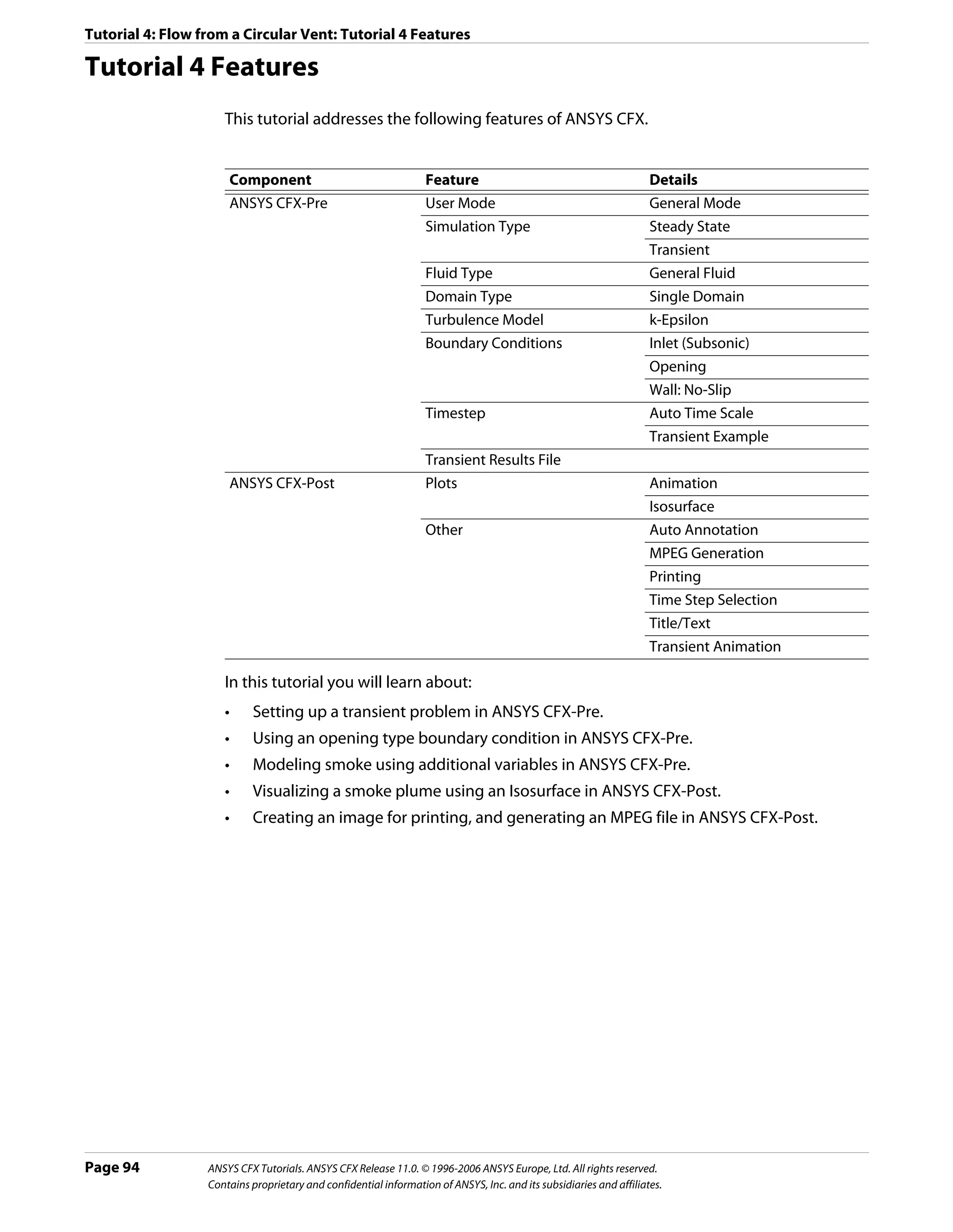

![Tutorial 4: Flow from a Circular Vent: Defining a Steady-State Simulation in ANSYS CFX-Pre
Importing the Mesh
1. Select File > Import Mesh.
2. From your working directory, select CircVentMesh.gtm.
3. Click Open.
4. Right-click a blank area in the viewer and select Predefined Camera > Isometric View
(Z up) from the shortcut menu.
Creating an Additional Variable
In this tutorial, an additional variable (non-reacting scalar component) will be used to model
the dispersion of smoke from the vent.
Note: While smoke is not required for the steady-state simulation, including it here prevents
the user from having to set up timevalue interpolation in the transient simulation.
1. From the main menu, select Insert > Expressions, Functions and Variables >
Additional Variable or click Additional Variable .
2. Under Name, type smoke.
3. Click OK.
4. Under Variable Type, select Volumetric.
5. Set Units to [kg m^-3].
6. Click OK.
Creating the Domain
The fluid domain will be created that includes the additional variable.
To Create a New 1. Select Insert > Domain from the main menu, or click Domain , then set the name to
Domain CircVent and click OK.
2. Apply the following settings
Tab Setting Value
General Options Fluids List Air at 25 C
Reference Pressure 0 [atm]
Fluid Models Heat Transfer > Option None
Additional Variable Details > smoke (Selected)
Additional Variable Details > smoke > (Selected)
Kinematic Diffusivity
Additional Variable Details > smoke > 1.0E-5 [m^2 s^-1]
Kinematic Diffusivity > Kinematic
Diffusivity
3. Click OK.
Page 96 ANSYS CFX Tutorials. ANSYS CFX Release 11.0. © 1996-2006 ANSYS Europe, Ltd. All rights reserved.
Contains proprietary and confidential information of ANSYS, Inc. and its subsidiaries and affiliates.](https://image.slidesharecdn.com/ansys11tutorial-111218135319-phpapp01/75/Ansys-11-tutorial-108-2048.jpg)
![Tutorial 4: Flow from a Circular Vent: Defining a Steady-State Simulation in ANSYS CFX-Pre
Creating the Boundary Conditions
This is an example of external flow, since fluid is flowing over an object and not through an
enclosure such as a pipe network (which would be an example of internal flow). In such
problems, some inlets will be made sufficiently large that they do not affect the CFD
solution. However, the length scale values produced by the Default Intensity and
AutoCompute Length Scale option for turbulence are based on inlet size. They are
appropriate for internal flow problems and particularly, cylindrical pipes. In general, you
need to set the turbulence intensity and length scale explicitly for large inlets in external
flow problems. If you do not have a value for the length scale, you can use a length scale
based on a typical length of the object, over which the fluid is flowing. In this case, you will
choose a turbulence length scale which is one-tenth of the diameter of the vent.
Note: The boundary marker vectors used to display boundary conditions (Inlets, Outlets,
Openings) are normal to the boundary surface regardless of the actual direction
specification. To plot vectors in the direction of flow, select Boundary Vector under the
Plot Options tab for the inlet boundary condition and clear Show Inlet Markers on the
Boundary Marker Options tab of Labels and Markers (accessible by clicking
Label and Marker Visibility ).
For parts of the boundary where the flow direction changes, or is unknown, an opening
boundary condition can be used. An opening boundary condition allows flow to both enter
and leave the fluid domain during the course of the solution.
Inlet Boundary 1. Select Insert > Boundary Condition from the main menu or click Boundary Condition
.
2. Under Name, type Wind.
3. Click OK.
4. Apply the following settings
Tab Setting Value
Basic Settings Boundary Type Inlet
Location Wind
Boundary Details Mass and Momentum > Option Cart. Vel. Components
Mass and Momentum > U 1 [m s^-1]
Mass and Momentum > V 0 [m s^-1]
Mass and Momentum > W 0 [m s^-1]
Turbulence > Option Intensity and Length Scale
Turbulence > Value 0.05
Turbulence > Eddy Len. Scale 0.25 [m]
Additional Variables > smoke > Option Value
Additional Variables > smoke > Value 0 [kg m^-3]
5. Click OK.
ANSYS CFX Tutorials. ANSYS CFX Release 11.0. © 1996-2006 ANSYS Europe, Ltd. All rights reserved. Page 97
Contains proprietary and confidential information of ANSYS, Inc. and its subsidiaries and affiliates.](https://image.slidesharecdn.com/ansys11tutorial-111218135319-phpapp01/75/Ansys-11-tutorial-109-2048.jpg)
![Tutorial 4: Flow from a Circular Vent: Defining a Steady-State Simulation in ANSYS CFX-Pre
Opening 1. Select Insert > Boundary Condition from the main menu or click Boundary Condition
Boundary .
2. Under Name, type Atmosphere.
3. Click OK.
4. Apply the following settings
Tab Setting Value
Basic Settings Boundary Type Opening
Location Atmosphere
Boundary Details Mass and Momentum > Option Opening Pres. and Dirn
Mass and Momentum > Relative Pressure 0 [Pa]
Flow Direction > Option Normal to Boundary
Condition
Turbulence > Option Intensity and Length Scale
Turbulence > Value 0.05
Turbulence > Eddy Len. Scale 0.25 [m]
Additional Variables > smoke > Option Value
Additional Variables > smoke > Value 0 [kg m^-3]
5. Click OK.
Inlet for the 1. Select Insert > Boundary Condition from the main menu or click Boundary Condition
Vent .
2. Under Name, type Vent.
3. Click OK.
4. Apply the following settings
Tab Setting Value
Basic Settings Boundary Type Inlet
Location Vent
Boundary Details Mass and Momentum > Normal Speed 0.01 [m s^-1]
Turbulence > Option Intensity and Eddy Viscosity
Ratio
Additional Variables > smoke > Option Value
Additional Variables > smoke > Value 0 [kg m^-3]
5. Click OK.
Setting Initial Values
1. Click Global Initialization .
2. Select Turbulence Eddy Dissipation.
3. Click OK.
Page 98 ANSYS CFX Tutorials. ANSYS CFX Release 11.0. © 1996-2006 ANSYS Europe, Ltd. All rights reserved.
Contains proprietary and confidential information of ANSYS, Inc. and its subsidiaries and affiliates.](https://image.slidesharecdn.com/ansys11tutorial-111218135319-phpapp01/75/Ansys-11-tutorial-110-2048.jpg)

![Tutorial 4: Flow from a Circular Vent: Defining a Transient Simulation in ANSYS CFX-Pre
Defining a Transient Simulation in ANSYS CFX-Pre
In this part of the tutorial, you alter the simulation settings used for the steady-state
calculation to set up the model for the transient calculation in ANSYS CFX-Pre.
Playing a Session File
If you wish to skip past these instructions, and have ANSYS CFX-Pre set up the simulation
automatically, you can select Session > Play Tutorial from the menu in ANSYS CFX-Pre,
then run the session file: CircVent.pre. After you have played the session file as described
in earlier tutorials under Playing the Session File and Starting ANSYS CFX-Solver Manager
(p. 87), proceed to Obtaining a Solution to the Transient Problem (p. 104).
Opening the Existing Simulation
1. Start ANSYS CFX-Pre.
2. Select File > Open Simulation.
3. If required, set the path location to the tutorial folder.
4. Select the simulation file CircVentIni.cfx.
5. Click Open.
6. Select File > Save Simulation As.
7. Change the name to CircVent.cfx.
8. Click Save.
Modifying the Simulation Type
In this step you will make the problem transient. Later, you will set the concentration of
smoke to rise exponentially with time, so it is necessary to ensure that the interval between
the timesteps is smaller at the beginning of the simulation than at the end.
1. Click Simulation Type .
2. Apply the following settings
Tab Setting Value
Basic Settings Simulation Type > Option Transient
Simulation Type > Time Duration > 30 [s]
Total Time
Simulation Type > Time Steps > 4*0.25, 2*0.5, 2*1.0, 13*2.0 [s]
Timesteps*†
Simulation Type > Initial Time > Time 0 [s]
*. Do NOT click Enter Expression to enter lists of values. Enter the list without the
units, then set the units in the drop-down list.
†. This list specifies 4 timesteps of 0.25 [s], then 2 timesteps of 0.5 [s], etc.
3. Click OK.
Page 100 ANSYS CFX Tutorials. ANSYS CFX Release 11.0. © 1996-2006 ANSYS Europe, Ltd. All rights reserved.
Contains proprietary and confidential information of ANSYS, Inc. and its subsidiaries and affiliates.](https://image.slidesharecdn.com/ansys11tutorial-111218135319-phpapp01/75/Ansys-11-tutorial-112-2048.jpg)
![Tutorial 4: Flow from a Circular Vent: Defining a Transient Simulation in ANSYS CFX-Pre
Modifying the Boundary Conditions
The only boundary condition which needs altering is the Vent boundary condition. In the
steady-state calculation, this boundary had a small amount of air flowing through it. In the
transient calculation, more air passes through the vent and there is a time-dependent
concentration of smoke in the air. This is initially zero, but builds up to a larger value. The
smoke concentration will be specified using the CFX Expression Language.
To Modify the 1. In the Outline workspace, expand the tree to Simulation > CircVent > Vent.
Vent Inlet 2. Right-click Vent and select Edit.
Boundary
Condition 3. Apply the following settings
Tab Setting Value
Boundary Details Mass and Momentum > Normal Speed 0.2 [m s^-1]
Leave the Vent details view open for now.
You are going to create an expression for smoke concentration. The concentration is
zero for time t=0 and builds up to a maximum of 1 kg m^-3.
4. Create a new expression by selecting Insert > Expressions, Functions and Variables
> Expression from the main menu. Set the name to TimeConstant.
5. Apply the following settings
Name Definition
TimeConstant 3 [s]
6. Click Apply to create the expression.
7. Create the following expressions with specific settings, remembering to click Apply
after each is defined.
Name Definition
FinalConcentration 1 [kg m^-3]
ExpFunction * FinalConcentration*abs(1-exp(-t/TimeConstant))
*. When entering this function, you can select most of the required items by
right-clicking in the Definition window in the Expression details view instead of
typing them. The names of the existing expressions are under the Expressions
menu. The exp and abs functions are under Functions > CEL. The variable t is
under Variables.
Note: The abs function takes the modulus (or magnitude) of its argument. Even though the
expression (1- exp (-t/TimeConstant)) can never be less than zero, the abs function is
included to ensure that the numerical error in evaluating it near to zero will never make the
expression evaluate to a negative number.
Next you will visualize how the expressions have scheduled the concentration of smoke
issued from the vent.
ANSYS CFX Tutorials. ANSYS CFX Release 11.0. © 1996-2006 ANSYS Europe, Ltd. All rights reserved. Page 101
Contains proprietary and confidential information of ANSYS, Inc. and its subsidiaries and affiliates.](https://image.slidesharecdn.com/ansys11tutorial-111218135319-phpapp01/75/Ansys-11-tutorial-113-2048.jpg)
![Tutorial 4: Flow from a Circular Vent: Defining a Transient Simulation in ANSYS CFX-Pre
Plotting Smoke 1. Double-click ExpFunction in the Expressions tree view.
Concentration 2. Apply the following settings
Tab Setting Value
Plot t (Selected)
Start of Range 0 [s]
End of Range 30 [s]
3. Click Plot Expression.
The button name then changes to Define Plot, as shown.
As can be seen, the smoke concentration rises exponentially, and reaches 90% of its final
value at around 7 seconds.
4. Click the Boundary: Vent tab.
In the next step, you will apply the expression ExpFunction to the additional variable
smoke as it applies to the boundary Vent.
5. Apply the following settings
Tab Setting Value
Boundary Details Additional Variables > smoke > Option Value
Additional Variables > smoke > Value* ExpFunction
*. Click Enter Expression to enter text.
6. Click OK.
Page 102 ANSYS CFX Tutorials. ANSYS CFX Release 11.0. © 1996-2006 ANSYS Europe, Ltd. All rights reserved.
Contains proprietary and confidential information of ANSYS, Inc. and its subsidiaries and affiliates.](https://image.slidesharecdn.com/ansys11tutorial-111218135319-phpapp01/75/Ansys-11-tutorial-114-2048.jpg)
![Tutorial 4: Flow from a Circular Vent: Defining a Transient Simulation in ANSYS CFX-Pre
Initialization Values
The steady state solution that you have finished calculating is used to supply the initial
values to the ANSYS CFX-Solver. You can leave all of the initialization data set to Automatic
and the initial values will be read automatically from the initial values file. Therefore, there
is no need to revisit the initialization tab.
Modifying the Solver Control
1. Click Solver Control .
2. Set Convergence Control > Max. Coeff. Loops to 3.
3. Leave the other settings at their default values.
4. Click OK to set the solver control parameters.
Output Control
To allow results to be viewed at different timesteps, it is necessary to create transient results
files at specified times. The transient results files do not have to contain all solution data. In
this step, you will create minimal transient results files.
To Create 1. From the main menu, select Insert > Solver > Output Control.
Minimal 2. Click the Trn Results tab.
Transient
Results Files 3. Click Add new item and then click OK to accept the default name for the object.
This creates a new transient results object. Each object can result in the production of
many transient results files.
4. Apply the following settings to Transient Results 1
Setting Value
Option Selected Variables
Output Variables List* Pressure, Velocity, smoke
Output Frequency > Option Time List
Output Frequency > Time List† 1, 2 , 3 [s]
*. Click the ellipsis icon to select items if they do not appear in the drop-down list. Use
the <Ctrl> key to select multiple items.
†. Do NOT click Enter Expression to enter lists of values. Enter the list without the
units, then set the units in the drop-down list.
5. Click Apply.
6. Create a second item with the default name Transient Results 2 and apply the
following settings to that item
Setting Value
Option Selected Variables
Output Variables List Pressure, Velocity, smoke
ANSYS CFX Tutorials. ANSYS CFX Release 11.0. © 1996-2006 ANSYS Europe, Ltd. All rights reserved. Page 103
Contains proprietary and confidential information of ANSYS, Inc. and its subsidiaries and affiliates.](https://image.slidesharecdn.com/ansys11tutorial-111218135319-phpapp01/75/Ansys-11-tutorial-115-2048.jpg)
![Tutorial 4: Flow from a Circular Vent: Obtaining a Solution to the Transient Problem
Setting Value
Output Frequency > Option Time Interval
Output Frequency > Time Interval* 4 [s]
*. A transient results file will be produced every 4 s (including 0 s) and at 1 s, 2 s and
3 s. The files will contain no mesh and data for only the three selected variables. This
reduces the size of the minimal results files. A full results file is always written at the
end of the run.
7. Click OK.
Writing the Solver (.def) File
1. Click Write Solver File .
2. Apply the following settings
Setting Value
File name CircVent.def
Quit CFX–Pre * Select
*. If using ANSYS CFX-Pre in Standalone Mode.
3. Ensure Start Solver Manager is selected and click Save.
4. Quit ANSYS CFX-Pre, saving the simulation (.cfx) file at your discretion.
Obtaining a Solution to the Transient Problem
In this tutorial the ANSYS CFX-Solver will read the initial values for the problem from a file.
For details, see Initialization Values (p. 103). You need to specify the file name.
Define Run will be displayed when the ANSYS CFX-Solver Manager launches. Definition
File will already be set to the name of the definition file just written.
Notice that the text output generated by the ANSYS CFX-Solver will be more than you have
seen for steady-state problems. This is because each timestep consists of several inner
(coefficient) iterations. At the end of each timestep, information about various quantities is
printed to the text output area.
The variable smoke is now plotted under the Additional Variables tab.
1. Under Initial Values File, click Browse .
2. Select CircVentIni_001.res, which is the results file of the steady-state problem with
no smoke issuing from the chimney. If you have not run the first part of this tutorial, copy
CircVentIni_001.res from the <CFXROOT>/examples/ directory to your working
directory.
3. Click Open.
4. Click Start Run.
5. You may see a notice that the mesh from the initial values file will be used. This mesh is
the same as in the definition file. Click OK to continue.
Page 104 ANSYS CFX Tutorials. ANSYS CFX Release 11.0. © 1996-2006 ANSYS Europe, Ltd. All rights reserved.
Contains proprietary and confidential information of ANSYS, Inc. and its subsidiaries and affiliates.](https://image.slidesharecdn.com/ansys11tutorial-111218135319-phpapp01/75/Ansys-11-tutorial-116-2048.jpg)
![Tutorial 4: Flow from a Circular Vent: Viewing the Results in ANSYS CFX-Post
ANSYS CFX-Solver runs and attempts to obtain a solution. This can take a long time
depending on your system. Eventually a dialog box is displayed.
6. When ANSYS CFX-Solver has finished, click Yes to post-process the results.
7. If using Standalone Mode, quit ANSYS CFX-Solver Manager.
Viewing the Results in ANSYS CFX-Post
In this tutorial, you will view the dispersion of smoke from the vent over time. When ANSYS
CFX-Post is loaded, the results that are immediately available are those at the final timestep;
in this case, at t = 30 s (this is nominally designated Final State).
Creating an Isosurface
An isosurface is a surface of constant value of a variable. For instance, it could be a surface
consisting of all points where the velocity is 1 [m s^-1]. In this case, you are going to create
an isosurface of smoke density (smoke is the additional variable that you specified earlier).
1. Right-click on a blank area in the viewer and select Predefined Camera > Isometric
View (Z up).
This ensures that the view is set to a position that is best suited to display the results.
2. From the main menu, select Insert > Location > Isosurface or under Location, click
Isosurface.
3. Click OK.
4. Apply the following settings
Tab Setting Value
Geometry Variable smoke
Value 0.005 [kg m^-3]
5. Click Apply.
• A bumpy surface will be displayed, showing the smoke starting to emerge from the
vent.
• The surface is rough because the mesh is coarse. For a smoother surface, you would
re-run the problem with a smaller mesh length scale.
• The surface will be a constant color as the default settings on the Color tab were
used.
• When Color Mode is set to either Constant or Use Plot Variable for an
isosurface, it appears as one color.
6. In Geometry, experiment by changing the Value so that you can see the shape of the
plume more clearly.
Zoom in and rotate the geometry, as required.
7. When you have finished, set the Value to 0.002 [kg m^-3].
8. Right-click on a blank spot in the viewer and select Predefined Camera > Isometric
View (Z up).
ANSYS CFX Tutorials. ANSYS CFX Release 11.0. © 1996-2006 ANSYS Europe, Ltd. All rights reserved. Page 105
Contains proprietary and confidential information of ANSYS, Inc. and its subsidiaries and affiliates.](https://image.slidesharecdn.com/ansys11tutorial-111218135319-phpapp01/75/Ansys-11-tutorial-117-2048.jpg)


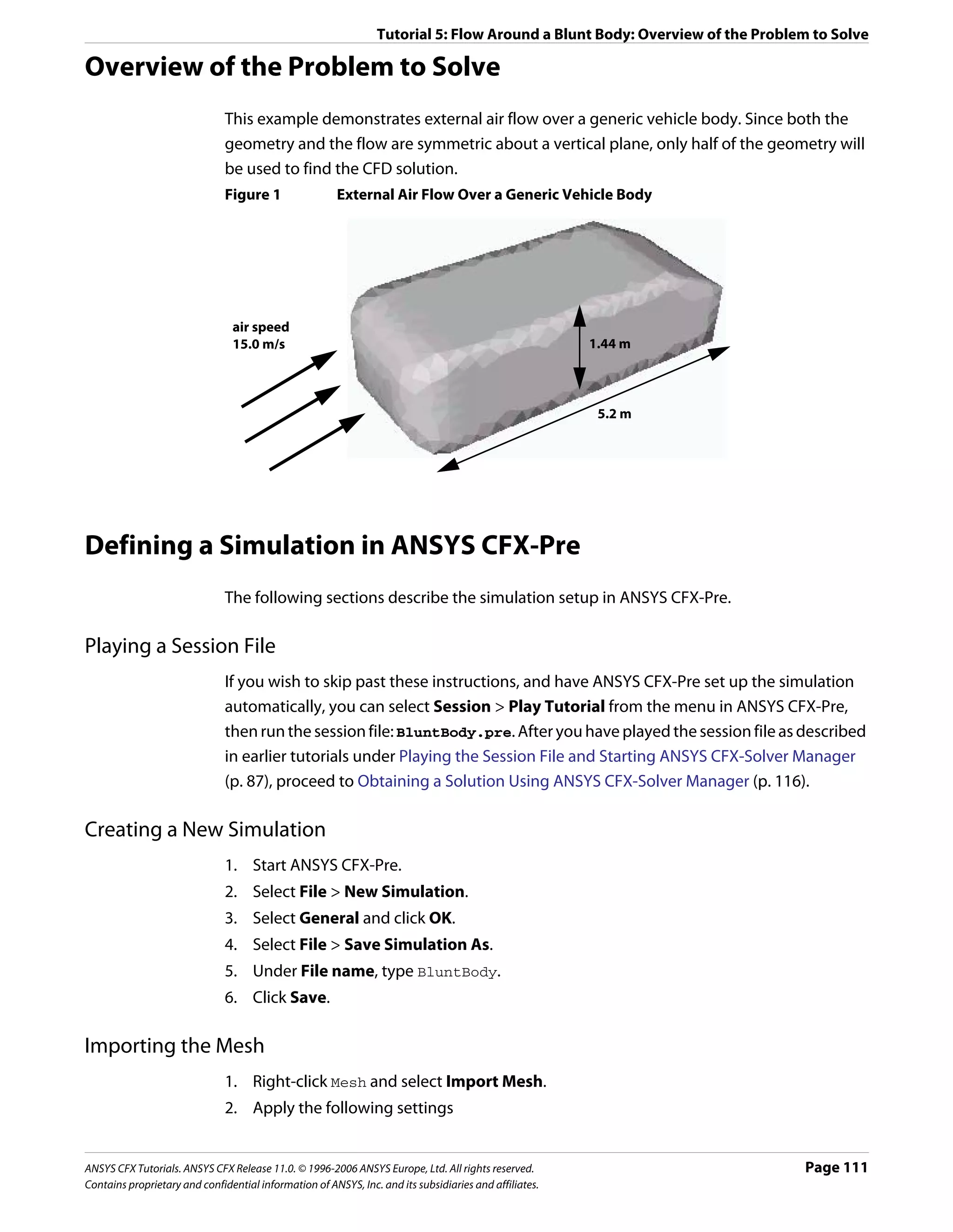
![Tutorial 5: Flow Around a Blunt Body: Defining a Simulation in ANSYS CFX-Pre
Setting Value
File name BluntBodyMesh.gtm
3. Click Open.
Creating the Domain
The flow in the domain is expected to be turbulent and approximately isothermal. The
Shear Stress Transport (SST) turbulence model with automatic wall function treatment will
be used because of its highly accurate predictions of flow separation. To take advantage of
the SST model, the boundary layer should be resolved with at least 10 mesh nodes. In order
to reduce computational time, the mesh in this tutorial is much coarser than that.
This tutorial uses an ideal gas as the fluid whereas previous tutorials have used a specific
fluid. When modeling a compressible flow using the ideal gas approximation to calculate
density variations, it is important to set a realistic reference pressure. This is because some
fluid properties depend on the absolute fluid pressure (calculated as the static pressure plus
the reference pressure).
1. Click Domain , and set the name to BluntBody.
2. Apply the following settings to BluntBody:
Tab Setting Value
General Options Basic Settings > Fluids List Air Ideal Gas
Domain Models > Pressure > Reference Pressure 1 [atm]
Fluid Models Heat Transfer > Option Isothermal
Heat Transfer > Fluid Temperature 288 [K]
Turbulence > Option Shear Stress Transport
3. Click OK.
Creating Composite Regions
An imported mesh may contain many 2D regions. For the purpose of creating boundary
conditions, it can sometimes be useful to group several 2D regions together and apply a
single boundary condition to the composite 2D region. In this case, you are going to create
a Union between two regions that both require a free slip wall boundary condition.
1. From the main menu, select Insert > Composite Region.
2. Set the name to FreeWalls and click OK.
3. Apply the following settings
Tab Setting Value
Basic Settings Dimension (Filter) 2D
4. In the region list, hold down the <Ctrl> key and select Free1 and Free2.
Page 112 ANSYS CFX Tutorials. ANSYS CFX Release 11.0. © 1996-2006 ANSYS Europe, Ltd. All rights reserved.
Contains proprietary and confidential information of ANSYS, Inc. and its subsidiaries and affiliates.](https://image.slidesharecdn.com/ansys11tutorial-111218135319-phpapp01/75/Ansys-11-tutorial-124-2048.jpg)
![Tutorial 5: Flow Around a Blunt Body: Defining a Simulation in ANSYS CFX-Pre
5. Click OK.
Creating the Boundary Conditions
The simulation requires inlet, outlet, wall (no slip and free slip) and symmetry plane
boundary conditions. The regions for these boundary conditions were defined when the
mesh was created (except for the composite region just created for the free slip wall
boundary condition).
Inlet Boundary 1. Click Boundary Condition .
2. Under Name, type Inlet.
3. Apply the following settings
Tab Setting Value
Basic Settings Boundary Type Inlet
Location Inlet
Boundary Details Flow Regime > Option Subsonic
Mass and Momentum > Option Normal Speed
Mass and Momentum > Normal Speed 15 [m s^-1]
Turbulence > Option Intensity and Length Scale
Turbulence > Eddy Len. Scale 0.1 [m]
4. Click OK.
Outlet 1. Create a new boundary condition named Outlet.
Boundary 2. Apply the following settings
Tab Setting Value
Basic Settings Boundary Type Outlet
Location Outlet
Boundary Details Mass and Momentum > Option Static Pressure
Mass and Momentum > Relative Pressure 0 [Pa]
3. Click OK.
Free Slip Wall The top and side surfaces of the rectangular region will use free slip wall boundary
Boundary conditions.
• On free slip walls the shear stress is set to zero so that the fluid is not retarded.
• The velocity normal to the wall is also set to zero.
• The velocity parallel to the wall is calculated during the solution.
This is not an ideal boundary condition for this situation since the flow around the body will
be affected by the close proximity to the walls. If this case was modeling a wind tunnel
experiment, the domain should model the size and shape of the wind tunnel and use no-slip
walls. If this case was modeling a blunt body open to the atmosphere, a much larger domain
should be used to minimize the effect of the walls.
ANSYS CFX Tutorials. ANSYS CFX Release 11.0. © 1996-2006 ANSYS Europe, Ltd. All rights reserved. Page 113
Contains proprietary and confidential information of ANSYS, Inc. and its subsidiaries and affiliates.](https://image.slidesharecdn.com/ansys11tutorial-111218135319-phpapp01/75/Ansys-11-tutorial-125-2048.jpg)

![Tutorial 5: Flow Around a Blunt Body: Defining a Simulation in ANSYS CFX-Pre
Tab Setting Value
Global Settings Initial Conditions > Cartesian Velocity Automatic with Value
Components > Option
Initial Conditions > Cartesian Velocity 15 [m s^-1]
Components > U
Initial Conditions > Cartesian Velocity 0 [m s^-1]
Components > V
Initial Conditions > Cartesian Velocity 0 [m s^-1]
Components > W
Initial Conditions > Turbulence Eddy (Selected)
Dissipation
3. Click OK.
Setting Solver Control
1. Click Solver Control .
2. Apply the following settings:
Tab Setting Value
Basic Settings Convergence Control > Max. Iterations 60
Convergence Control > Fluid Timescale Control > Physical Timescale
Timescale Control
Convergence Control > Fluid Timescale Control > 2 [s]
Physical Timescale
Convergence Criteria > Residual Target 1e-05
3. Click OK.
Writing the Solver (.def) File
1. Click Write Solver File .
2. Apply the following settings:
Setting Value
File name BluntBody.def
Quit CFX–Pre* (Selected)
*. If using ANSYS CFX-Pre in Standalone Mode.
3. Ensure Start Solver Manager is selected and click Save.
4. If using Standalone Mode, quit ANSYS CFX-Pre, saving the simulation (.cfx) file at your
discretion.
ANSYS CFX Tutorials. ANSYS CFX Release 11.0. © 1996-2006 ANSYS Europe, Ltd. All rights reserved. Page 115
Contains proprietary and confidential information of ANSYS, Inc. and its subsidiaries and affiliates.](https://image.slidesharecdn.com/ansys11tutorial-111218135319-phpapp01/75/Ansys-11-tutorial-127-2048.jpg)

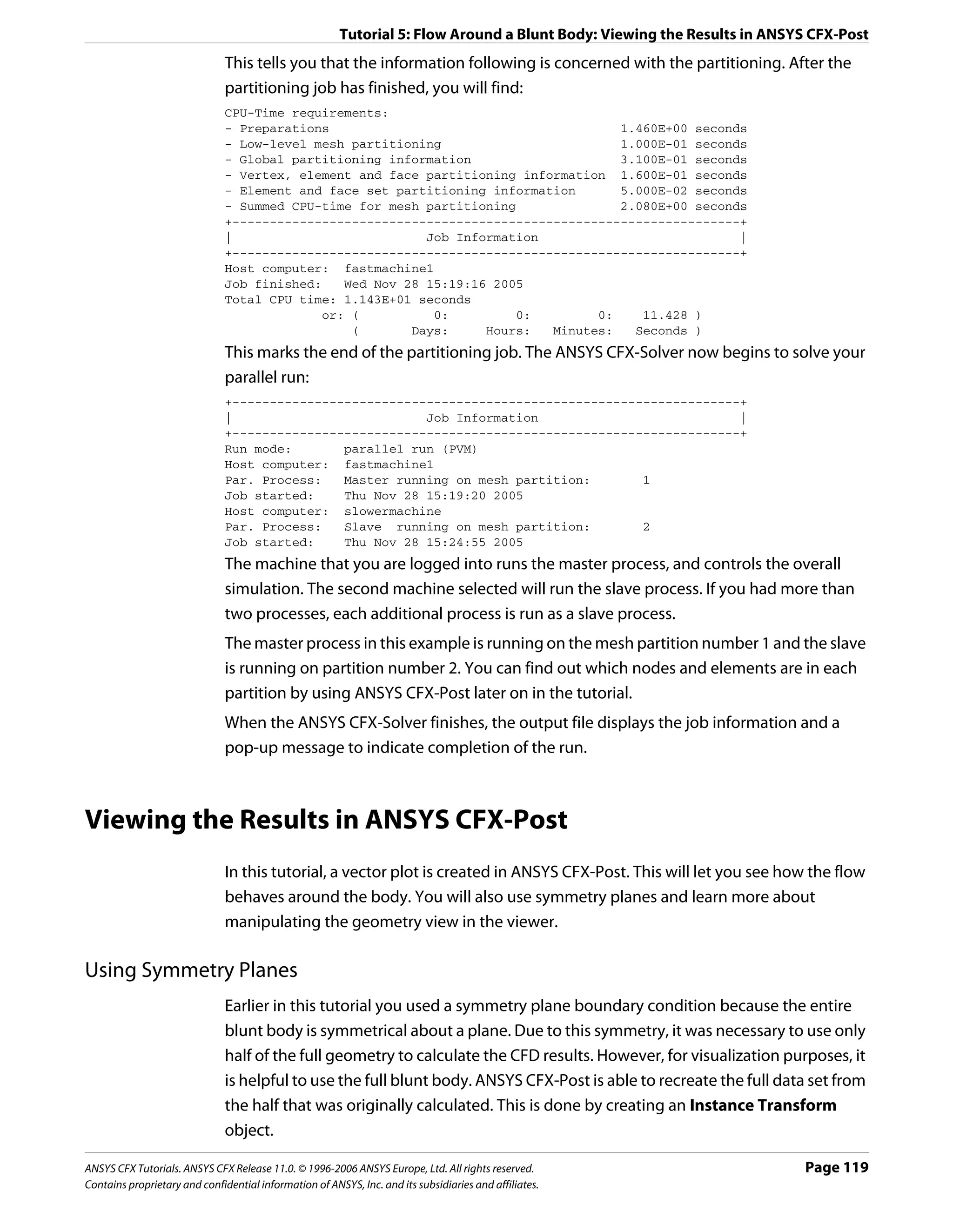

![Tutorial 5: Flow Around a Blunt Body: Viewing the Results in ANSYS CFX-Post
Creating Vectors
You are now going to create a vector plot to show velocity vectors behind the blunt body.
You need to first create an object to act as a locator, which, in this case, will be a sampling
plane. Then, create the vector plot itself.
Creating the A sampling plane is a plane with evenly spaced sampling points on it.
Sampling Plane
1. Right-click a blank area in the viewer and select Predefined Camera > View Towards
+Y.
This ensures that the changes can be seen.
2. Create a new plane named Sample.
3. Apply the following settings:
Tab Setting Value
Geometry Definition > Method Point and Normal
Definition > Point 6, -0.001, 1
Definition > Normal 0, 1, 0
Plane Bounds > Type Rectangular
Plane Bounds > X Size 2.5 [m]
Plane Bounds > Y Size 2.5 [m]
Plane Type Sample
Plane Type > X Samples 20
Plane Type > Y Samples 20
Render Draw Faces (Cleared)
Draw Lines (Selected)
4. Click Apply.
You can zoom in on the sampling plane to see the location of the sampling points
(where lines intersect). There are a total of 400 (20 * 20) sampling points on the plane. A
vector can be created at each sampling point.
5. Hide the plane by clearing the visibility check box next to Sample.
Creating a 1. Click Vector and accept the default name.
Vector Plot 2. Apply the following settings:
Using Different
Sampling
Methods Tab Setting Value
Geometry Definition > Locations Sample
Definition > Sampling Vertex
Symbol Symbol Size 0.25
3. Click Apply.
4. Zoom until the vector plot is roughly the same size as the viewer.
You should be able to see a region of recirculation behind the blunt body.
ANSYS CFX Tutorials. ANSYS CFX Release 11.0. © 1996-2006 ANSYS Europe, Ltd. All rights reserved. Page 121
Contains proprietary and confidential information of ANSYS, Inc. and its subsidiaries and affiliates.](https://image.slidesharecdn.com/ansys11tutorial-111218135319-phpapp01/75/Ansys-11-tutorial-133-2048.jpg)
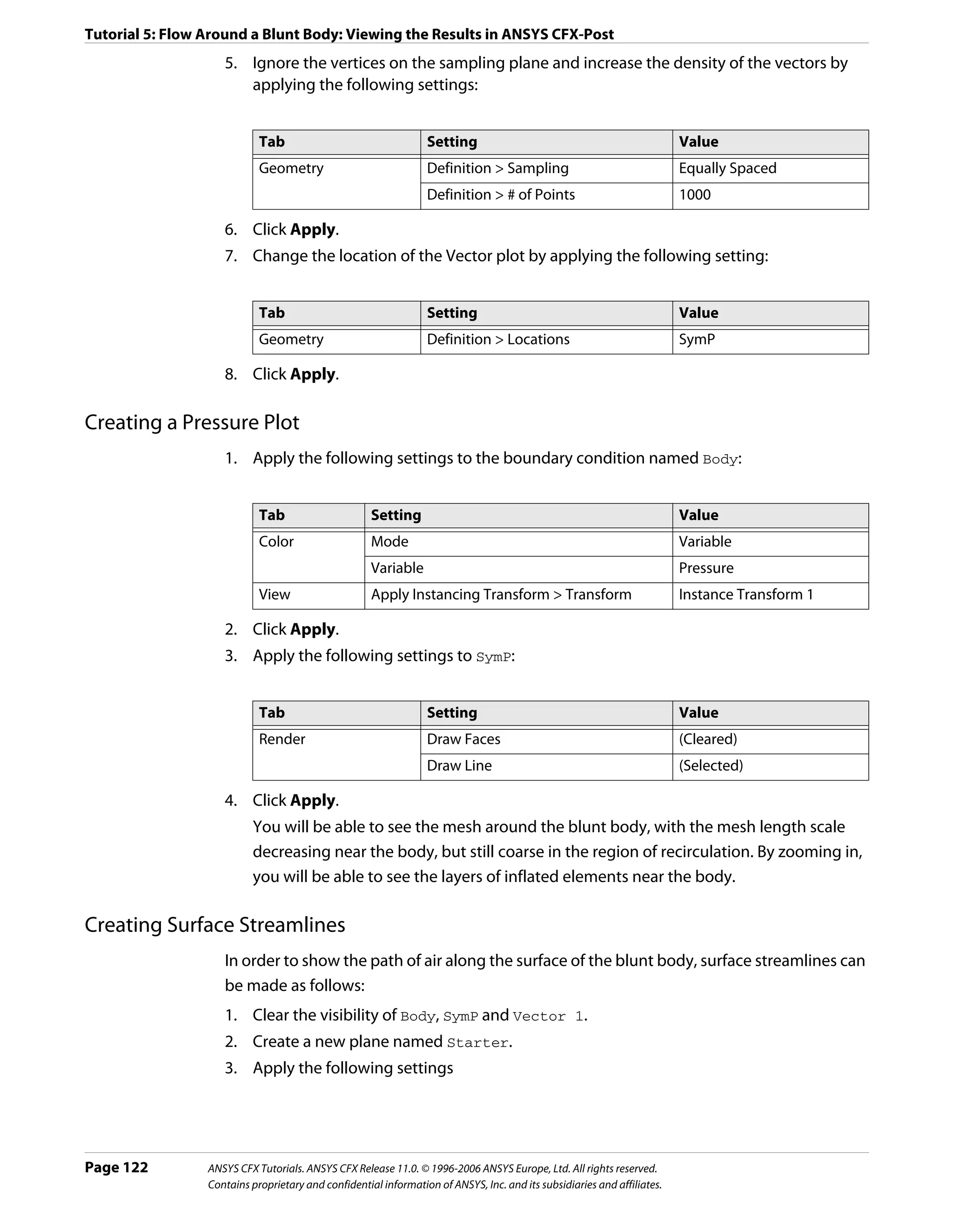
![Tutorial 5: Flow Around a Blunt Body: Viewing the Results in ANSYS CFX-Post
Tab Setting Value
Geometry Definition > Method YZ Plane
X -0.1 [m]
4. Click Apply.
The plane appears just upstream of the blunt body.
5. Clear the visibility check box for the plane.
This hides the plane from view, although the plane still exists.
6. Click Streamline . and click OK to accept the default name.
7. Apply the following settings:
Tab Setting Value
Geometry Type Surface Streamline
Definition > Surfaces Body
Definition > Start From Locations
Definition > Locations Starter
Definition > Max Points 100
Definition > Direction Forward
8. Apply the following settings.
The surface streamlines appear on half of the surface of the blunt body. They start near
the upstream end because the starting points were formed by projecting nodes from
the plane to the blunt body.
Moving Objects
In ANSYS CFX-Post, you can reposition some locator objects directly in the viewer by using
the mouse.
1. Select the visibility check box for the plane named Starter.
2. Select the Single Select mouse pointer from the Selection Tools toolbar.
3. In the viewer, click the Starter plane to select it, then use the left mouse button to drag
it along the X axis.
Notice that the streamlines are redrawn as the plane moves.
Creating a Surface Plot of y+
The velocity next to a no-slip wall boundary changes rapidly from a value of zero at the wall
to the free stream value a short distance away from the wall. This layer of high velocity
gradient is known as the boundary layer. Many meshes are not fine enough near a wall to
accurately resolve the velocity profile in the boundary layer. Wall functions can be used in
these cases to apply an assumed functional shape of the velocity profile. Other grids are fine
enough that they do not require wall functions, and application of the latter has little effect.
ANSYS CFX Tutorials. ANSYS CFX Release 11.0. © 1996-2006 ANSYS Europe, Ltd. All rights reserved. Page 123
Contains proprietary and confidential information of ANSYS, Inc. and its subsidiaries and affiliates.](https://image.slidesharecdn.com/ansys11tutorial-111218135319-phpapp01/75/Ansys-11-tutorial-135-2048.jpg)
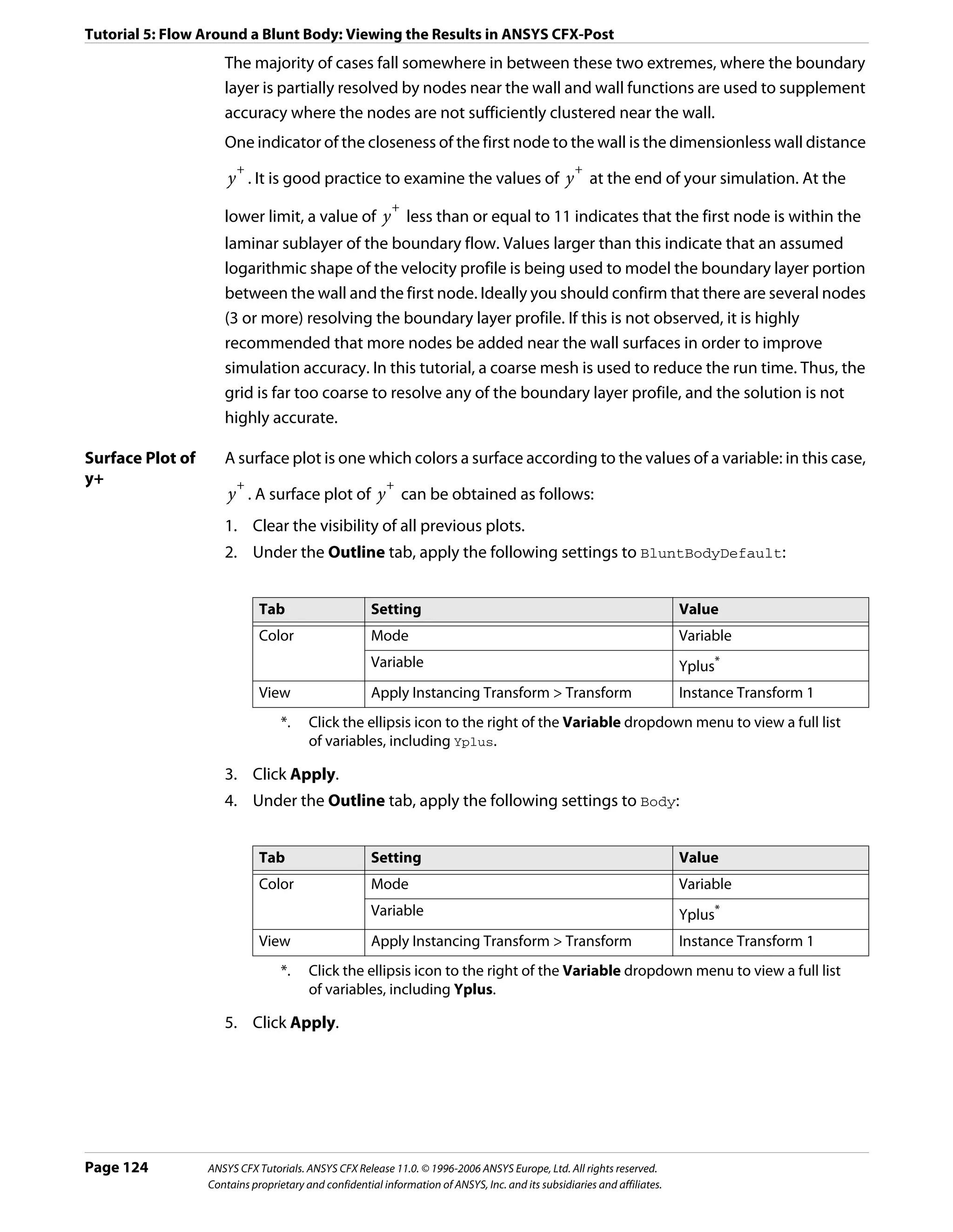
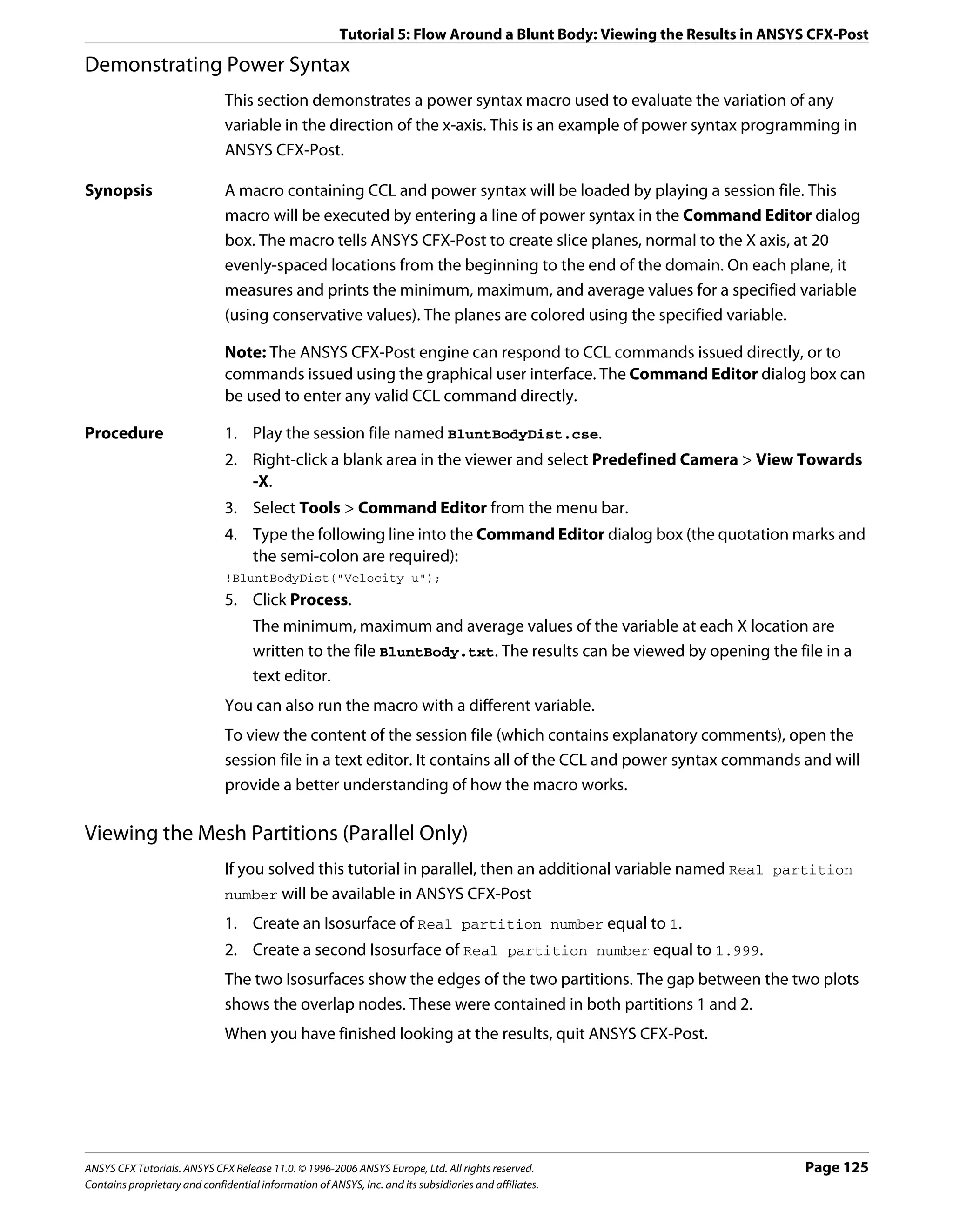
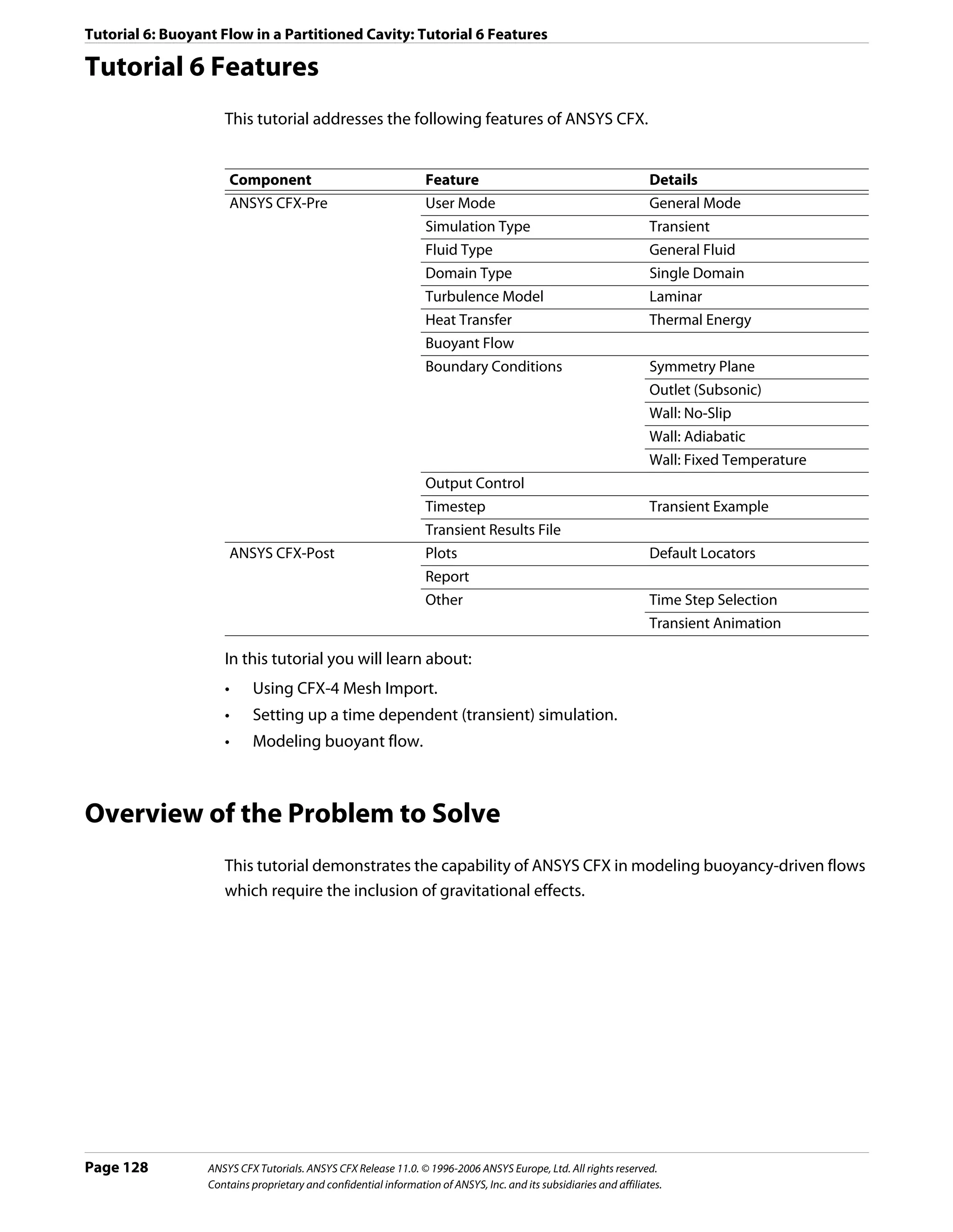

![Tutorial 6: Buoyant Flow in a Partitioned Cavity: Defining a Simulation in ANSYS CFX-Pre
2. Apply the following settings
Setting Value
File type CFX-4
File name Buoyancy2D.geo*
*. This file is in your tutorial directory.
3. Click Open.
Simulation Type
The default units and coordinate frame settings are suitable for this tutorial, but the
simulation type needs to be set to transient.
You will notice physics validation messages as the case is set to Transient. These errors will
be fixed in the later part of the tutorial.
1. Click Simulation Type .
2. Apply the following settings
Tab Setting Value
Basic Settings Simulation Type > Option Transient
Simulation Type > Time Duration > 2 [s]
Total Time*
Simulation Type > Time Steps > 0.025 [s]
Timesteps†
Simulation Type > Initial Time > Time 0 [s]
*. This is the total duration, in real time, for the simulation
†. This is the interval from one step, in real time, to the next. The simulation will
continue, moving forward in time by 0.025 s, until the total time has been reached
3. Click OK.
Page 130 ANSYS CFX Tutorials. ANSYS CFX Release 11.0. © 1996-2006 ANSYS Europe, Ltd. All rights reserved.
Contains proprietary and confidential information of ANSYS, Inc. and its subsidiaries and affiliates.](https://image.slidesharecdn.com/ansys11tutorial-111218135319-phpapp01/75/Ansys-11-tutorial-142-2048.jpg)
![Tutorial 6: Buoyant Flow in a Partitioned Cavity: Defining a Simulation in ANSYS CFX-Pre
Creating the Domain
gsin30
30
gcos30
g
y
x
30
You will model the cavity as if it were tilted at an angle of 30°. You can do this by specifying
horizontal and vertical components of the gravity vector, which are aligned with the default
coordinate axes, as shown in the diagram above.
To Create a New 1. Click Domain , and set the name to Buoyancy2D.
Domain 2. Apply the following settings to Buoyancy2D
Tab Setting Value
General Basic Settings > Fluids List Air at 25 C
Options Domain Models > Pressure > Reference Pressure 1 [atm]
Domain Models > Buoyancy > Option Buoyant
Domain Models > Buoyancy > Gravity X Dirn. -4.9 [m s^-2]
Domain Models > Buoyancy > Gravity Y Dirn. -8.5 [m s^-2]
Domain Models > Buoyancy > Gravity Z Dirn. 0.0 [m s^-2]*
Domain Models > Buoyancy > Buoy. Ref. Temp. 40 [C]†
Fluid Models Heat Transfer > Option Thermal Energy
Turbulence > Option None (Laminar)
*. This produces a gravity vector which simulates the tilt of the cavity
†. Do not forget to change the units. This is just an approximate representative
domain temperature.
Initialization will be set up using Global Initialization , so there is no need to visit the
Initialization tab.
3. Click OK.
ANSYS CFX Tutorials. ANSYS CFX Release 11.0. © 1996-2006 ANSYS Europe, Ltd. All rights reserved. Page 131
Contains proprietary and confidential information of ANSYS, Inc. and its subsidiaries and affiliates.](https://image.slidesharecdn.com/ansys11tutorial-111218135319-phpapp01/75/Ansys-11-tutorial-143-2048.jpg)
![Tutorial 6: Buoyant Flow in a Partitioned Cavity: Defining a Simulation in ANSYS CFX-Pre
Creating the Boundary Conditions
Hot and Cold You will create a wall boundary condition with a fixed temperature of 75 C on the bottom
Wall Boundary surface of the cavity, as follows:
1. Create a new boundary condition named hot.
2. Apply the following settings
Tab Setting Value
Basic Settings Boundary Type Wall
Location WALLHOT
Boundary Heat Transfer > Option Temperature
Details
Heat Transfer > Fixed Temperature 75 [C]
3. Click OK.
4. Create a new boundary condition named cold.
5. Apply the following settings
Tab Setting Value
Basic Settings Boundary Type Wall
Location WALLCOLD
Boundary Heat Transfer > Option Temperature
Details Heat Transfer > Fixed Temperature 5 [C]
6. Click OK.
Symmetry Plane A single symmetry plane boundary condition can be used for the front and back of the
Boundary cavity.
1. Create a new boundary condition named SymP.
2. Apply the following settings
Tab Setting Value
Basic Settings Boundary Type Symmetry
Location SYMMET1, SYMMET2*
*. Use the <Ctrl> key to select more than one region.
3. Click OK.
The default adiabatic wall boundary condition will automatically be applied to the
remaining boundaries.
Setting Initial Values
You should set initial settings using the Automatic with Value option when defining a
transient simulation. Using this option, the first run will use the specified initial conditions
while subsequent runs will use results file data for initial conditions.
Page 132 ANSYS CFX Tutorials. ANSYS CFX Release 11.0. © 1996-2006 ANSYS Europe, Ltd. All rights reserved.
Contains proprietary and confidential information of ANSYS, Inc. and its subsidiaries and affiliates.](https://image.slidesharecdn.com/ansys11tutorial-111218135319-phpapp01/75/Ansys-11-tutorial-144-2048.jpg)
![Tutorial 6: Buoyant Flow in a Partitioned Cavity: Defining a Simulation in ANSYS CFX-Pre
1. Click Global Initialization .
2. Apply the following settings
Tab Setting Value
Global Settings Initial Conditions > Cartesian Velocity Automatic with
Components > Option Value
Initial Conditions > Cartesian Velocity 0 [m s^-1]
Components > U
Initial Conditions > Cartesian Velocity 0 [m s^-1]
Components > V
Initial Conditions > Cartesian Velocity 0 [m s^-1]
Components > W
Initial Conditions > Static Pressure > Relative 0 [Pa]
Pressure
Initial Conditions > Temperature > Temperature 5 [C]
3. Click OK.
Setting Output Control
1. Click Output Control .
2. Click the Trn Results tab.
3. Create a new Transient Results item with the default name.
4. Apply the following settings
Tab Setting Value
Trn Results Transient Results > Transient Results 1 > Selected Variables
Option
Transient Results > Transient Results 1 > Pressure, Temperature,
Output Variables List* Velocity
Transient Results > Transient Results 1 > Time Interval
Output Frequency > Option
Transient Results > Transient Results 1 > 0.1 [s]
Output Frequency > Time Interval
*. Click the ellipsis icon to select items if they do not appear in the drop-down list. Use
the <Ctrl> key to select multiple items.
5. Click OK.
Setting Solver Control
1. Click Solver Control .
2. Apply the following settings
ANSYS CFX Tutorials. ANSYS CFX Release 11.0. © 1996-2006 ANSYS Europe, Ltd. All rights reserved. Page 133
Contains proprietary and confidential information of ANSYS, Inc. and its subsidiaries and affiliates.](https://image.slidesharecdn.com/ansys11tutorial-111218135319-phpapp01/75/Ansys-11-tutorial-145-2048.jpg)
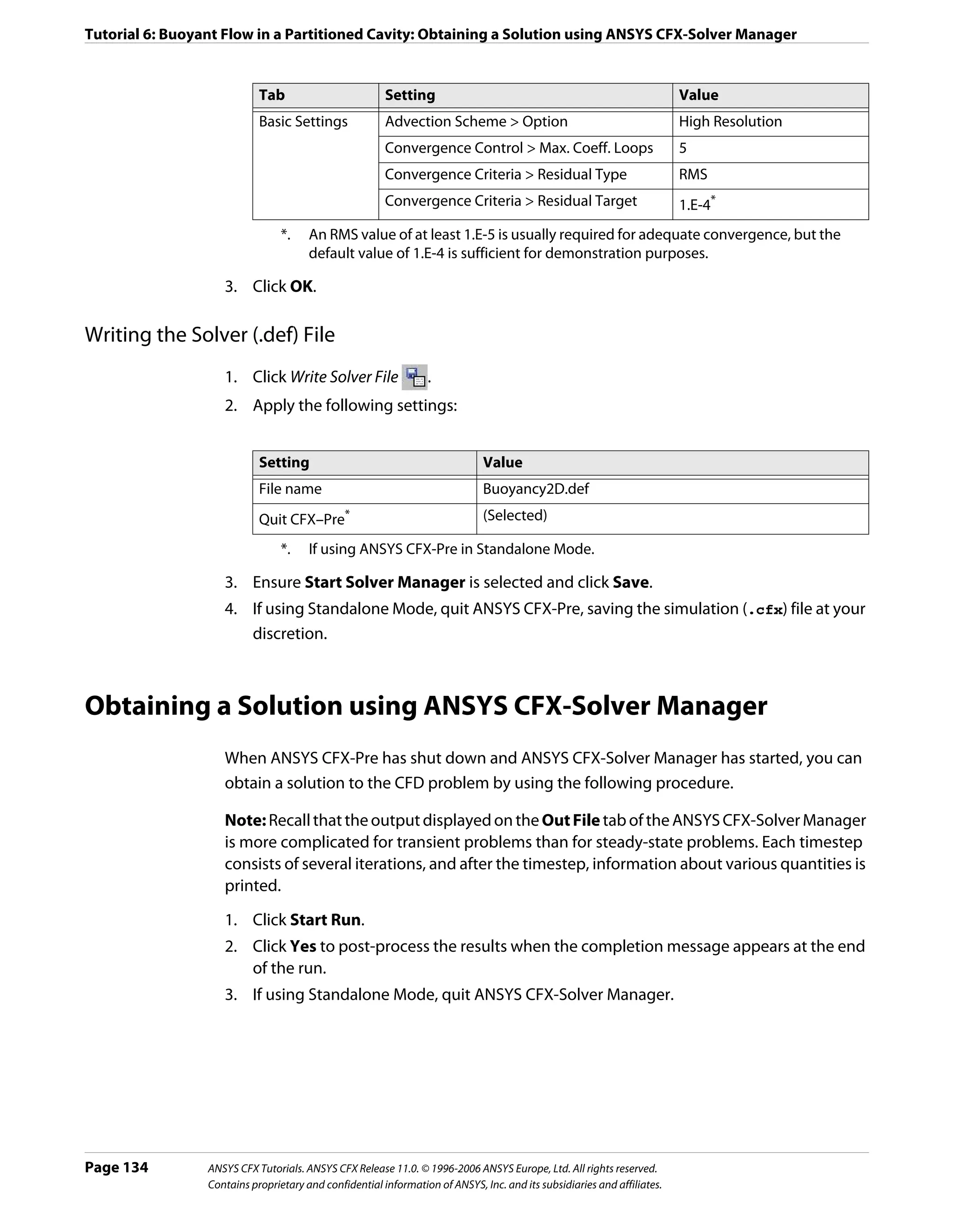


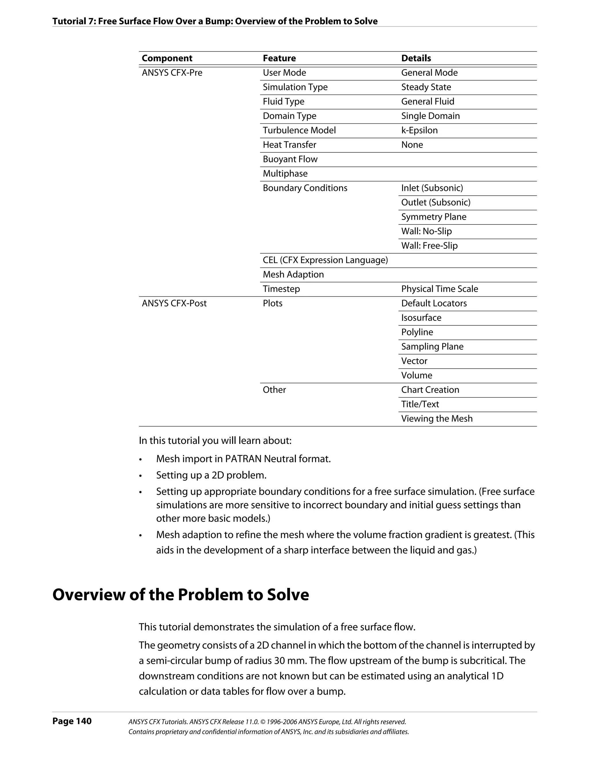
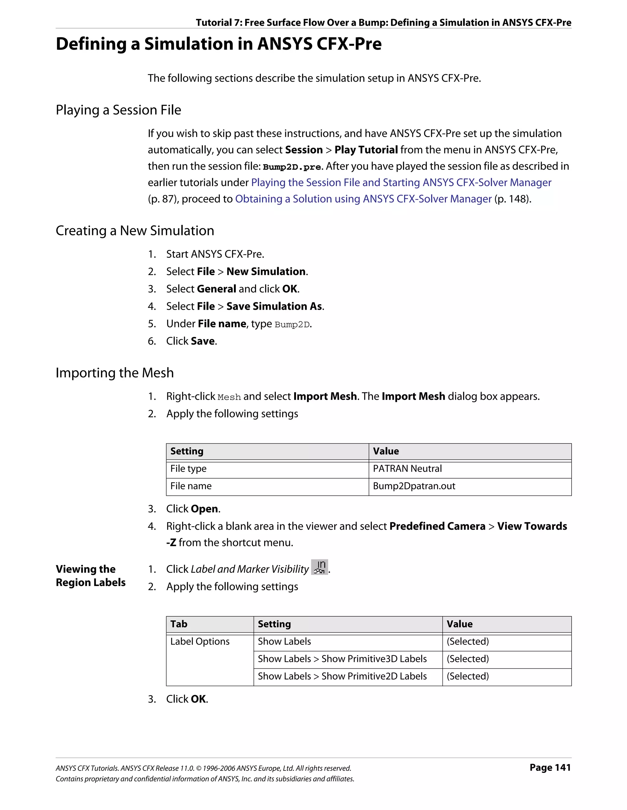
![Tutorial 7: Free Surface Flow Over a Bump: Defining a Simulation in ANSYS CFX-Pre
Creating Expressions for Initial and Boundary Conditions
Simulation of free surface flows usually requires defining boundary and initial conditions to
set up appropriate pressure and volume fraction fields. You will need to create expressions
using CEL (CFX Expression Language) to define these conditions.
In this simulation, the following conditions are set and require expressions:
• An inlet boundary where the volume fraction above the free surface is 1 for air and 0 for
water, and below the free surface is 0 for air and 1 for water.
• A pressure-specified outlet boundary, where the pressure above the free surface is
constant and the pressure below the free surface is a hydrostatic distribution. This
requires you to know the approximate height of the fluid at the outlet. In this case, an
analytical solution for 1D flow over a bump was used. The simulation is not sensitive to
the exact outlet fluid height, so an approximation is sufficient. You will examine the
effect of the outlet boundary condition in the post-processing section and confirm that
it does not affect the validity of the results. It is necessary to specify such a boundary
condition to force the flow downstream of the bump into the supercritical regime.
• An initial pressure field for the domain with a similar pressure distribution to that of the
outlet boundary.
Either create expressions using the Expressions workspace or import expressions from a
file.
• Creating Expressions (p. 142)
• Reading Expressions From a File (p. 143)
Creating 1. Right-click Expressions in the tree view and select Insert > Expression.
Expressions 2. Set the name to UpH and click OK.
3. Set Definition to 0.069 [m], and then click Apply.
4. Use the same method to create the expressions listed in the table below. These are
expressions for the downstream free surface height, the density of the fluid, the
upstream volume fractions of air and water, the upstream pressure distribution, the
downstream volume fractions of air and water, and the downstream pressure
distribution.
Name Definition
DownH 0.022 [m]
DenH 998 [kg m^-3]
UpVFAir step((y-UpH)/1[m])
UpVFWater 1-UpVFAir
UpPres DenH*g*UpVFWater*(UpH-y)
DownVFAir step((y-DownH)/1[m])
DownVFWater 1-DownVFAir
DownPres DenH*g*DownVFWater*(DownH-y)
5. Proceed to Creating the Domain (p. 143).
Page 142 ANSYS CFX Tutorials. ANSYS CFX Release 11.0. © 1996-2006 ANSYS Europe, Ltd. All rights reserved.
Contains proprietary and confidential information of ANSYS, Inc. and its subsidiaries and affiliates.](https://image.slidesharecdn.com/ansys11tutorial-111218135319-phpapp01/75/Ansys-11-tutorial-154-2048.jpg)
![Tutorial 7: Free Surface Flow Over a Bump: Defining a Simulation in ANSYS CFX-Pre
Reading 1. Copy the file Bump2DExpressions.ccl to your working directory from the ANSYS CFX
Expressions examples directory.
From a File 2. Select File > Import CCL.
3. When Import CCL appears, ensure that Append is selected.
4. Select Bump2DExpressions.ccl.
5. Click Open.
6. After the file has been imported, use the Expression tree view to view the expressions
that have been created.
Creating the Domain
1. Right click Simulation in the Outline tree view and ensure that Automatic Default
Domain is selected. A domain named Default Domain should now appear under the
Simulation branch.
2. Double click Default Domain and apply the following settings
Tab Setting Value
General Basic Settings > Fluids List Air at 25 C, Water
Options Domain Models > Pressure > Reference Pressure 1 [atm]
Domain Models > Buoyancy > Option Buoyant
Domain Models > Buoyancy > Gravity X Dirn. 0 [m s^-2]
Domain Models > Buoyancy > Gravity Y Dirn.* -g
Domain Models > Buoyancy > Gravity Z Dirn. 0 [m s^-2]
Domain Models > Buoyancy > Buoy. Ref. Density† 1.185 [kg m^-3]
Domain Models > Buoyancy > Ref Location > Option Automatic
Fluid Models Multiphase Options > Homogeneous Model‡ (Selected)
Multiphase Options > Free Surface Model > Option Standard
Heat Transfer > Option Isothermal
Heat Transfer > Fluid Temperature 25 C
Turbulence > Option k-Epsilon
*. You need to click Enter Expression beside the field first.
†. Always set Buoyancy Reference Density to the density of the least dense fluid in free
surface calculations.
‡. The homogeneous model solves for a single solution field. This is only appropriate
in some simulations.
3. Click OK.
Creating the Boundary Conditions
Inlet Boundary 1. Create a new boundary condition named inflow.
2. Apply the following settings
ANSYS CFX Tutorials. ANSYS CFX Release 11.0. © 1996-2006 ANSYS Europe, Ltd. All rights reserved. Page 143
Contains proprietary and confidential information of ANSYS, Inc. and its subsidiaries and affiliates.](https://image.slidesharecdn.com/ansys11tutorial-111218135319-phpapp01/75/Ansys-11-tutorial-155-2048.jpg)
![Tutorial 7: Free Surface Flow Over a Bump: Defining a Simulation in ANSYS CFX-Pre
Tab Setting Value
Basic Boundary Type Inlet
Settings
Location INFLOW
Boundary Mass and Momentum > Option Normal Speed
Details
Mass and Momentum > Option > Normal Speed 0.26 [m s^-1]
Turbulence > Option Intensity and Length Scale
Turbulence > Value 0.05
Turbulence > Eddy Len. Scale* UpH
Fluid Values Boundary Conditions Air as 25 C
Air at 25 C > Volume Fraction > Volume Fraction UpVFAir
Boundary Conditions Water
Water > Volume Fraction > Volume Fraction UpVFWater
*. Click the Enter Expression icon.
3. Click OK.
Outlet 1. Create a new boundary condition named outflow.
Boundary 2. Apply the following settings
Tab Setting Value
Basic Boundary Type Outlet
Settings Location OUTFLOW
Boundary Flow Regime> Option Subsonic
Details Mass and Momentum > Option Static Pressure
Mass and Momentum > Relative Pressure DownPres
3. Click OK.
Symmetry 1. Create a new boundary condition named front.
Boundary 2. Apply the following settings
Tab Setting Value
Basic Boundary Type Symmetry
Settings
Location FRONT
3. Click OK.
4. Create a new boundary condition named back.
5. Apply the following settings
Tab Setting Value
Basic Boundary Type Symmetry
Settings
Location BACK
Page 144 ANSYS CFX Tutorials. ANSYS CFX Release 11.0. © 1996-2006 ANSYS Europe, Ltd. All rights reserved.
Contains proprietary and confidential information of ANSYS, Inc. and its subsidiaries and affiliates.](https://image.slidesharecdn.com/ansys11tutorial-111218135319-phpapp01/75/Ansys-11-tutorial-156-2048.jpg)
![Tutorial 7: Free Surface Flow Over a Bump: Defining a Simulation in ANSYS CFX-Pre
6. Click OK.
Wall and 1. Create a new boundary condition named top.
Opening 2. Apply the following settings
Boundaries
Tab Setting Value
Basic Settings Boundary Type Opening
Location TOP
Boundary Details Mass And Momentum > Option Static Pres. (Entrain)
Mass And Momentum > Relative Pressure 0 [Pa]
Turbulence > Option Zero Gradient
Fluid Values Boundary Conditions Air at 25 C
Boundary Conditions > Air at 25 C > 1.0
Volume Fraction > Volume Fraction
Boundary Conditions Water
Boundary Conditions > Water > Volume 0.0
Fraction > Volume Fraction
3. Click OK.
4. Create a new boundary condition named bottom.
5. Apply the following settings
Tab Setting Value
Basic Boundary Type Wall
Settings Location BOTTOM1, BOTTOM2, BOTTOM3
Boundary Wall Influence on Flow > Option No Slip
Details Wall Roughness > Option Smooth Wall
6. Click OK.
Setting Initial Values
1. Click Global Initialization .
2. Apply the following settings
ANSYS CFX Tutorials. ANSYS CFX Release 11.0. © 1996-2006 ANSYS Europe, Ltd. All rights reserved. Page 145
Contains proprietary and confidential information of ANSYS, Inc. and its subsidiaries and affiliates.](https://image.slidesharecdn.com/ansys11tutorial-111218135319-phpapp01/75/Ansys-11-tutorial-157-2048.jpg)
![Tutorial 7: Free Surface Flow Over a Bump: Defining a Simulation in ANSYS CFX-Pre
Tab Setting Value
Global Settings Initial Conditions > Cartesian Velocity Automatic with Value
Components > Option
Initial Conditions > Cartesian Velocity 0.26 [m s^-1]
Components > U
Initial Conditions > Cartesian Velocity 0 [m s^-1]
Components > V
Initial Conditions > Cartesian Velocity 0 [m s^-1]
Components > W
Initial Conditions > Static Pressure > Option Automatic with Value
Initial Conditions > Static Pressure > Relative UpPres
Pressure
Initial Conditions > Turbulence Eddy Dissipation (Selected)
Fluid Settings Fluid Specific Initialization > Air at 25 C (Selected)
Air at 25 C > Initial Conditions > Volume Fraction > Automatic with Value
Option
Air at 25 C > Initial Conditions > Volume Fraction > UpVFAir
Volume Fraction
Fluid Settings Fluid Specific Initialization > Water (Selected)
Fluid Specific Initialization > Water > Initial Automatic with Value
Conditions > Volume Fraction > Option
Fluid Specific Initialization > Water > Initial UpVFWater
Conditions > Volume Fraction > Volume Fraction
3. Click OK.
Setting Mesh Adaption Parameters
1. Click Mesh Adaption .
2. Apply the following settings
Tab Setting Value
Basic Settings Activate Adaption (Selected)
Save Intermediate Files (Cleared)
Adaption Criteria > Variables List Air at 25 C.Volume Fraction
Adaption Criteria > Max. Num. Steps 2
Adaption Criteria > Option Multiple of Initial Mesh
Adaption Criteria > Node Factor 4
Adaption Convergence Criteria > Max. 100
Iter. per Step
Advanced Options Node Alloc. Param. 1.6
Number of Levels 2
3. Click OK.
Page 146 ANSYS CFX Tutorials. ANSYS CFX Release 11.0. © 1996-2006 ANSYS Europe, Ltd. All rights reserved.
Contains proprietary and confidential information of ANSYS, Inc. and its subsidiaries and affiliates.](https://image.slidesharecdn.com/ansys11tutorial-111218135319-phpapp01/75/Ansys-11-tutorial-158-2048.jpg)
![Tutorial 7: Free Surface Flow Over a Bump: Defining a Simulation in ANSYS CFX-Pre
Setting Solver Control
Important: Setting Max Iterations to 200 and Number of Adaption Levels to 2 with a
maximum of 100 timesteps each, results in a total maximum number of timesteps of 400
(2*100+200=400).
1. Click Solver Control .
2. Apply the following settings
Tab Setting Value
Basic Settings Convergence Control > Max. Iterations 200
Convergence Control >Fluid Timescale Physical Timescale
Control > Timescale Control
Convergence Control >Fluid Timescale 0.25 [s]
Control > Physical Timescale
Advanced Options Multiphase Control (Selected)
Multiphase Control > Volume Fraction (Selected)
Coupling
Multiphase Control > Volume Fraction Coupled
Coupling > Option
Note: The options selected above activate the Coupled Volume Fraction solution algorithm.
This algorithm typically converges better than the Segregated Volume Faction algorithm for
buoyancy-driven problems such as this tutorial, which requires a 0.05 [s] timescale using the
Segregated Volume Faction algorithm compared with 0.25 [s] for the Coupled Volume
Fraction algorithm.
Note:
3. Click OK.
Writing the Solver (.def) File
1. Click Write Solver File .
2. Apply the following settings:
Setting Value
File name Bump2D.def
Quit CFX–Pre* (Selected)
*. If using ANSYS CFX-Pre in Standalone Mode.
3. Ensure Start Solver Manager is selected and click Save.
4. If using Standalone Mode, quit ANSYS CFX-Pre, saving the simulation (.cfx) file at your
discretion.
ANSYS CFX Tutorials. ANSYS CFX Release 11.0. © 1996-2006 ANSYS Europe, Ltd. All rights reserved. Page 147
Contains proprietary and confidential information of ANSYS, Inc. and its subsidiaries and affiliates.](https://image.slidesharecdn.com/ansys11tutorial-111218135319-phpapp01/75/Ansys-11-tutorial-159-2048.jpg)
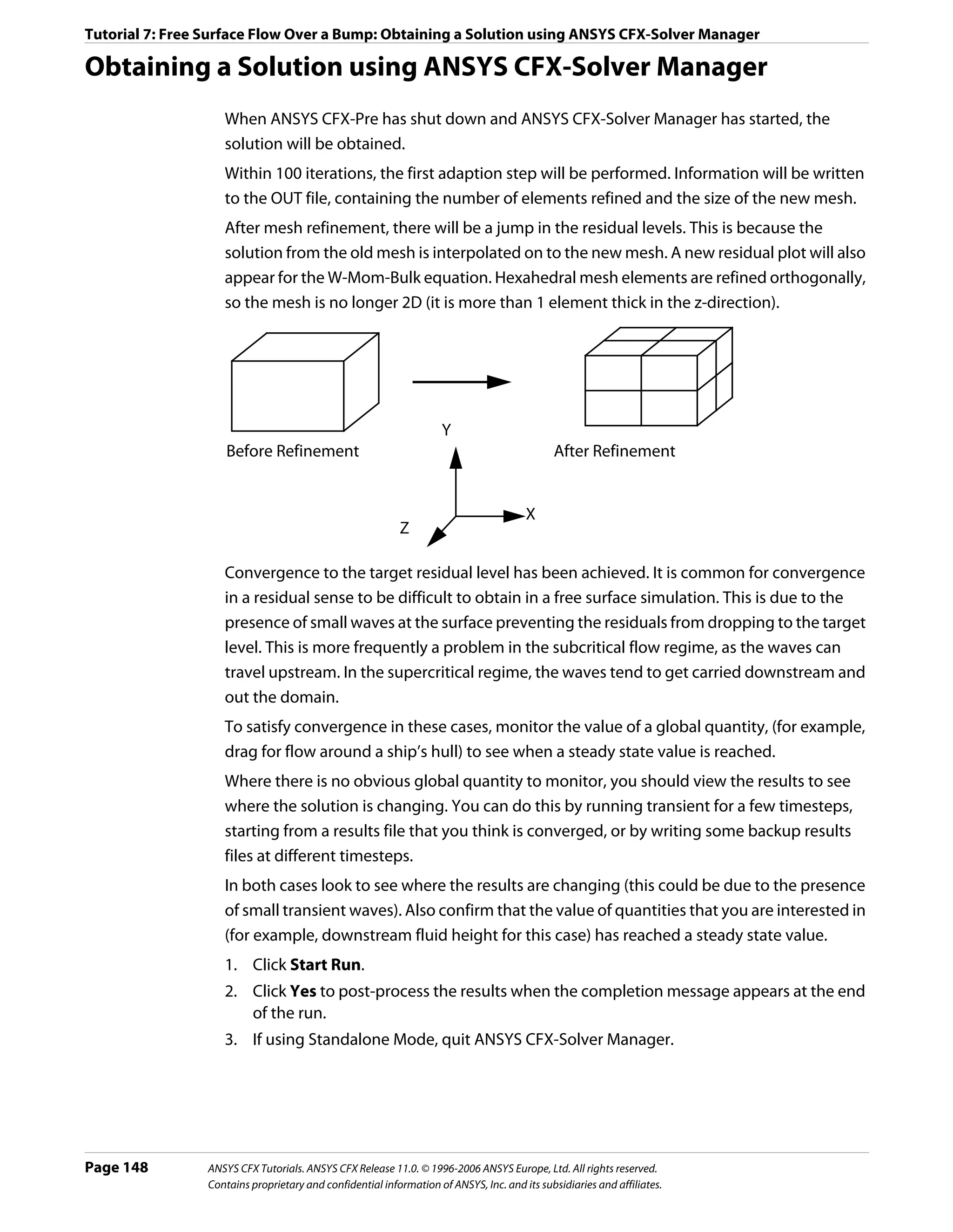
![Tutorial 7: Free Surface Flow Over a Bump: Viewing the Results in ANSYS CFX-Post
Viewing the Results in ANSYS CFX-Post
1. Select View Towards -Z by right-clicking on a blank area in the viewer and selecting
Predefined Camera > View Towards -Z.
2. Zoom in so the geometry fills the Viewer.
3. In the tree view under Bump2D, edit front.
4. Apply the following settings
Tab Setting Value
Color Mode Variable
Variable Water.Volume Fraction
5. Click Apply.
6. Clear the check box next to front.
Creating Velocity Vector Plots
The next step involves creating a sampling plane to display velocity vectors for Water.
1. Create a new plane named Plane 1.
2. Apply the following settings
Tab Setting Value
Geometry Definition > Method XY Plane
Plane Bounds > Type Rectangular
Plane Bounds > X Size 1.25 [m]
Plane Bounds > Y Size 0.3 [m]
Plane Bounds > X Angle 0 [degree]
Plane Type Sample
X Samples 160
Y Samples 40
Render Draw Faces (Cleared)
Draw Lines (Selected)
3. Click Apply.
4. Clear the check box next to Plane 1.
5. Create a new vector named Vector 1.
6. Apply the following settings
Tab Setting Value
Geometry Definition > Locations Plane 1
Definition > Variable * Water.Velocity
Symbol Symbol Size 0.5
ANSYS CFX Tutorials. ANSYS CFX Release 11.0. © 1996-2006 ANSYS Europe, Ltd. All rights reserved. Page 149
Contains proprietary and confidential information of ANSYS, Inc. and its subsidiaries and affiliates.](https://image.slidesharecdn.com/ansys11tutorial-111218135319-phpapp01/75/Ansys-11-tutorial-161-2048.jpg)
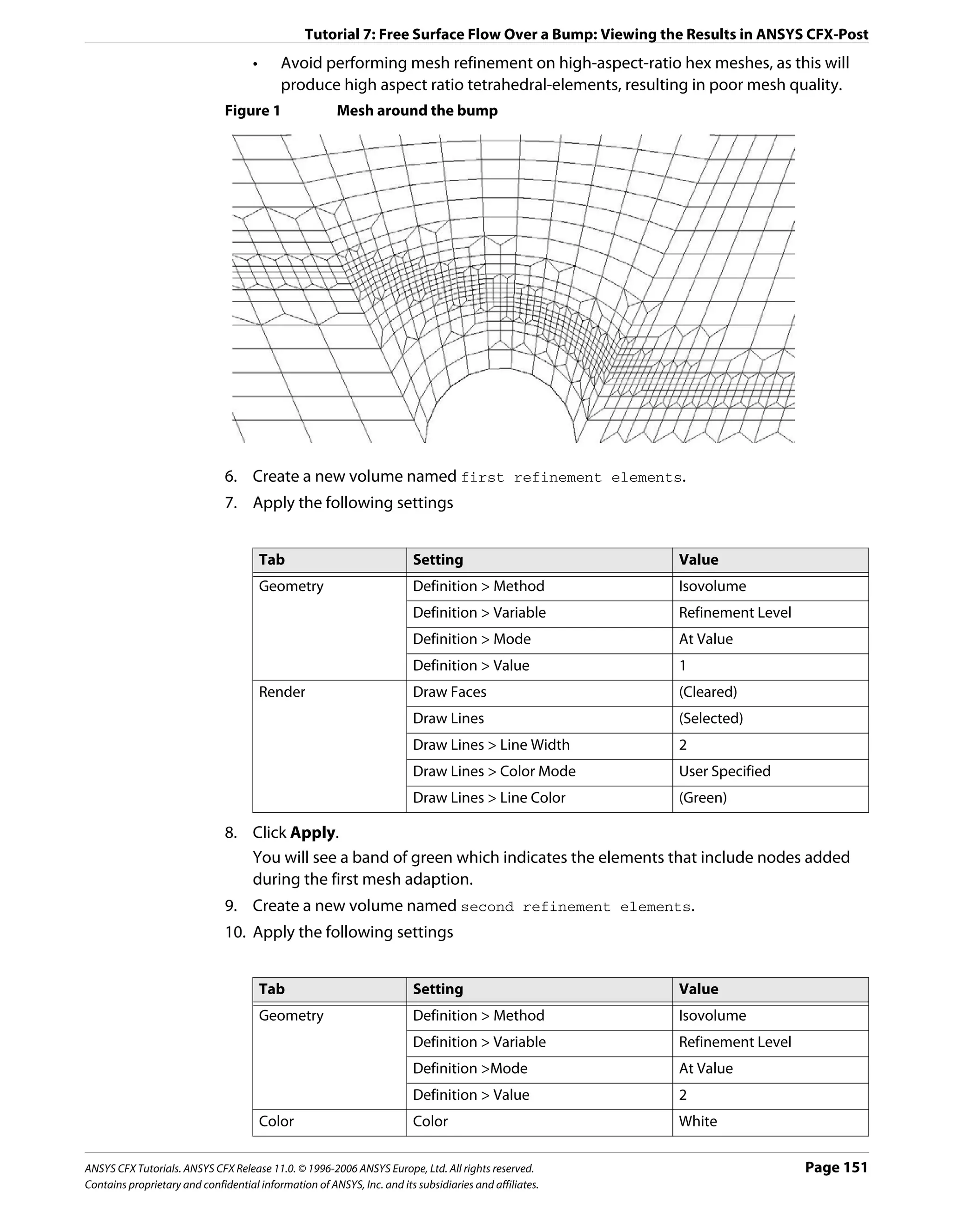
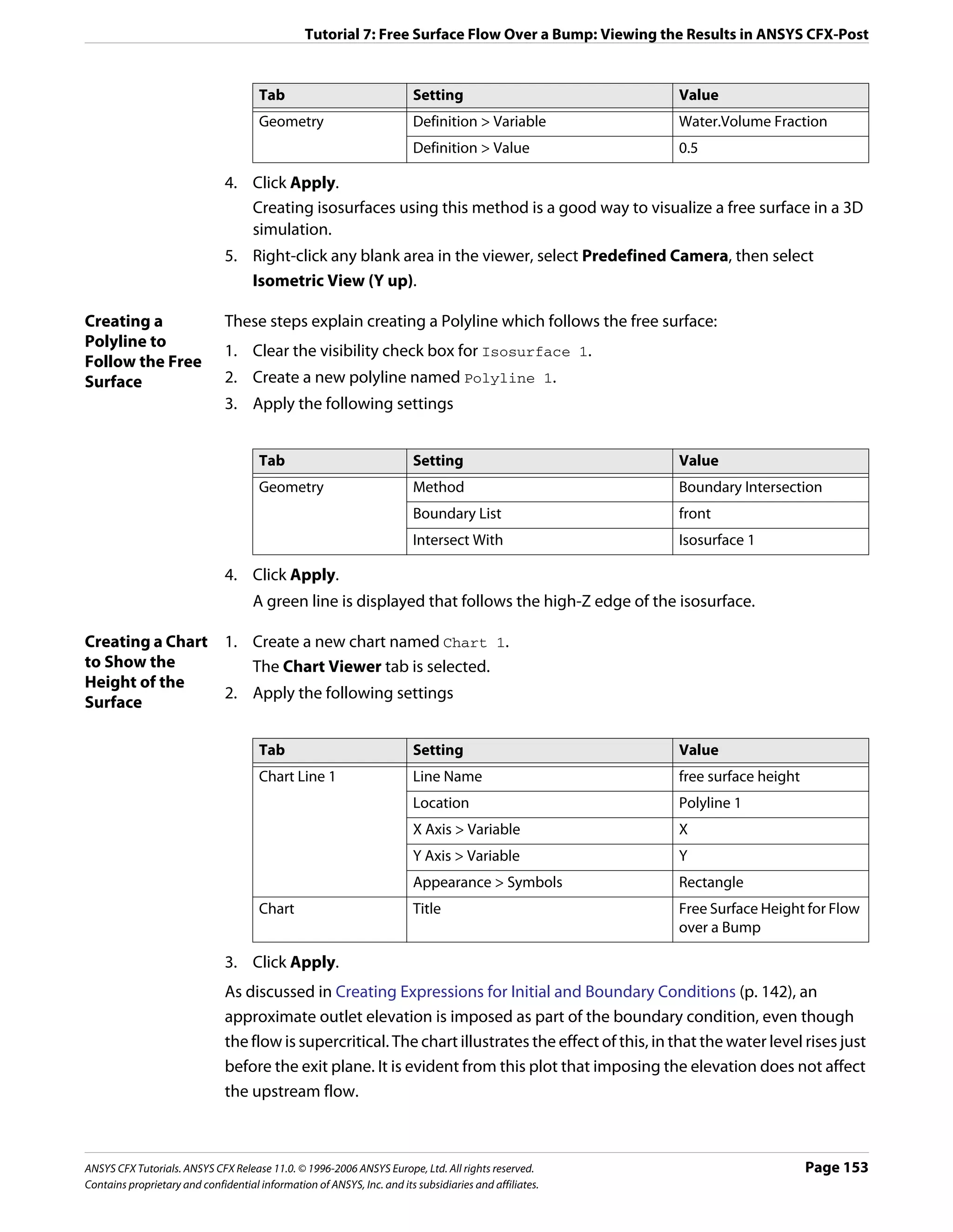
![Tutorial 7: Free Surface Flow Over a Bump: Using a Supercritical Outlet Condition
The chart shows a wiggle in the elevation of the free surface interface at the inlet. This is
related to an overspecification of conditions at the inlet, since both the inlet velocity and
elevation were specified. For a subcritical inlet, only the velocity or the total energy should
be specified. The wiggle is due to a small inconsistency between the specified elevation and
the elevation computed by the solver to obtain critical conditions at the bump. The wiggle
is analogous to one found if pressure and velocity were both specified at a subsonic inlet, in
a converging-diverging nozzle with choked flow at the throat.
Further Post-processing
You may wish to create some plots using the <Fluid>.Superficial Velocity variables.
This is the fluid volume fraction multiplied by the fluid velocity and is sometimes called the
volume flux. It is useful to use this variable for vector plots in separated multiphase flow, as
you will only see a vector where a significant amount of that phase exists.
Using a Supercritical Outlet Condition
For supercritical free surface flows, the supercritical outlet boundary condition is usually the
most appropriate boundary condition for the outlet, since it does not rely on the
specification of the outlet pressure distribution (which depends on an estimate of the free
surface height at the outlet). The supercritical outlet boundary condition requires a relative
pressure specification for the gas only; no pressure information is required for the liquid at
the outlet. For this tutorial, the relative gas pressure at the outlet should be set to 0 [Pa].
The supercritical outlet condition may admit multiple solutions. To find the supercritical
solution, it is often necessary to start with a static pressure outlet condition (as previously
done in this tutorial) or an average static pressure condition where the pressure is set
consistent with an elevation to drive the solution into the supercritical regime. The outlet
condition can then be changed to the supercritical option.
Page 154 ANSYS CFX Tutorials. ANSYS CFX Release 11.0. © 1996-2006 ANSYS Europe, Ltd. All rights reserved.
Contains proprietary and confidential information of ANSYS, Inc. and its subsidiaries and affiliates.](https://image.slidesharecdn.com/ansys11tutorial-111218135319-phpapp01/75/Ansys-11-tutorial-166-2048.jpg)

![Tutorial 8: Supersonic Flow Over a Wing: Overview of the Problem to Solve
Overview of the Problem to Solve
This example demonstrates the use of ANSYS CFX in simulating supersonic flow over a
symmetric NACA0012 airfoil at 0° angle of attack. A 2D section of the wing is modeled. A 2D
hexahedral mesh is provided that is imported into ANSYS CFX-Pre.
air speed 1.25 [m]
u = 600 m/s
outlet
30 [m]
wing surface
70 [m]
Defining a Simulation in ANSYS CFX-Pre
The following sections describe the simulation setup in ANSYS CFX-Pre.
Playing a Session File
If you wish to skip past these instructions, and have ANSYS CFX-Pre set up the simulation
automatically, you can select Session > Play Tutorial from the menu in ANSYS CFX-Pre,
then run the session file: WingSPS.pre. After you have played the session file as described
in earlier tutorials under Playing the Session File and Starting ANSYS CFX-Solver Manager
(p. 87), proceed to Obtaining a Solution using ANSYS CFX-Solver Manager (p. 162).
Creating a New Simulation
1. Start ANSYS CFX-Pre.
2. Select File > New Simulation.
3. Select General and click OK.
4. Select File > Save Simulation As.
5. Under File name, type WingSPS.
6. Click Save.
ANSYS CFX Tutorials. ANSYS CFX Release 11.0. © 1996-2006 ANSYS Europe, Ltd. All rights reserved. Page 157
Contains proprietary and confidential information of ANSYS, Inc. and its subsidiaries and affiliates.](https://image.slidesharecdn.com/ansys11tutorial-111218135319-phpapp01/75/Ansys-11-tutorial-169-2048.jpg)
![Tutorial 8: Supersonic Flow Over a Wing: Defining a Simulation in ANSYS CFX-Pre
Importing the Mesh
1. Right-click Mesh and select Import Mesh. The Import Mesh dialog box appears.
2. Apply the following settings
Setting Value
File type PATRAN Neutral
File name WingSPSMesh.out
3. Click Open.
4. Right-click a blank area in the viewer and select Predefined Camera > Isometric View
(Y up) from the shortcut menu.
Creating the Domain
Creating a New 1. Right click Simulation in the Outline tree view and ensure that Automatic Default
Domain Domain is selected. A domain named Default Domain should now appear under the
Simulation branch.
2. Double click it and apply the following settings
Tab Setting Value
General Options Basic Settings > Location WING
Fluids List Air Ideal Gas
Domain Models > Pressure > 1 [atm]
Reference Pressure*
Fluid Models Heat Transfer > Option Total Energy†
Turbulence > Option Shear Stress Transport
*. When using an ideal gas, it is important to set an appropriate reference pressure
since some properties depend on the absolute pressure level.
†. The Total Energy model is appropriate for high speed flows since it includes kinetic
energy effects.
3. Click OK.
Creating the Boundary Conditions
Inlet Boundary 1. Create a new boundary condition named Inlet.
2. Apply the following settings
Tab Setting Value
Basic Settings Boundary Type Inlet
Location INLET
Page 158 ANSYS CFX Tutorials. ANSYS CFX Release 11.0. © 1996-2006 ANSYS Europe, Ltd. All rights reserved.
Contains proprietary and confidential information of ANSYS, Inc. and its subsidiaries and affiliates.](https://image.slidesharecdn.com/ansys11tutorial-111218135319-phpapp01/75/Ansys-11-tutorial-170-2048.jpg)
![Tutorial 8: Supersonic Flow Over a Wing: Defining a Simulation in ANSYS CFX-Pre
Tab Setting Value
Boundary Details Flow Regime > Option Supersonic
Mass and Momentum > Option Cart. Vel. & Pressure
Mass and Momentum > U 600 [m s^-1]
Mass and Momentum > V 0 [m s^-1]
Mass and Momentum > W 0 [m s^-1]
Mass and Momentum > Rel. Static Pres. 0 [Pa]
Turbulence > Option Intensity and Length Scale
Turbulence > Value 0.01
Turbulence > Eddy Len. Scale 0.02 [m]
Heat Transfer > Static Temperature 300 [K]
3. Click OK.
Outlet 1. Create a new boundary condition named Outlet.
Boundary 2. Apply the following settings
Tab Setting Value
Basic Settings Boundary Type Outlet
Location OUTLET
Boundary Details Flow Regime > Option Supersonic
3. Click OK.
Symmetry Plane 1. Create a new boundary condition named SymP1.
Boundary 2. Apply the following settings
Tab Setting Value
Basic Settings Boundary Type Symmetry
Location SIDE1
3. Click OK.
4. Create a new boundary condition named SymP2.
5. Apply the following settings
Tab Setting Value
Basic Settings Boundary Type Symmetry
Location SIDE2
6. Click OK.
7. Create a new boundary condition named Bottom.
8. Apply the following settings
ANSYS CFX Tutorials. ANSYS CFX Release 11.0. © 1996-2006 ANSYS Europe, Ltd. All rights reserved. Page 159
Contains proprietary and confidential information of ANSYS, Inc. and its subsidiaries and affiliates.](https://image.slidesharecdn.com/ansys11tutorial-111218135319-phpapp01/75/Ansys-11-tutorial-171-2048.jpg)
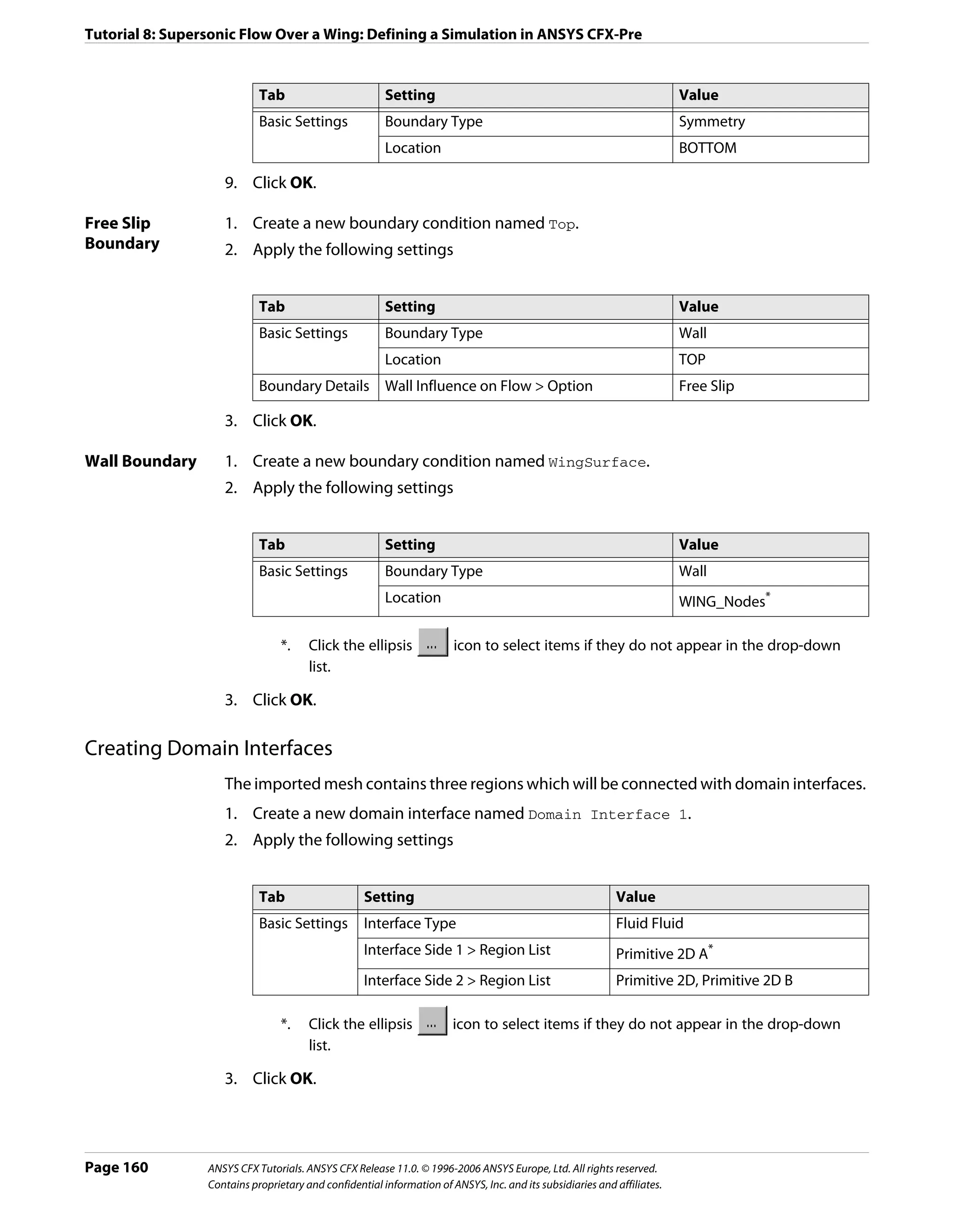
![Tutorial 8: Supersonic Flow Over a Wing: Defining a Simulation in ANSYS CFX-Pre
Setting Initial Values
For high speed compressible flow, the ANSYS CFX-Solver usually requires sensible initial
conditions to be set for the velocity field.
1. Click Global Initialization .
2. Apply the following settings
Tab Setting Value
Global Initial Conditions > Cartesian Velocity Components > Option Automatic
Settings with Value
Initial Conditions > Cartesian Velocity Components > U 600 [m s^-1]
Initial Conditions > Cartesian Velocity Components > V 0 [m s^-1]
Initial Conditions > Cartesian Velocity Components > W 0 [m s^-1]
Initial Conditions > Temperature > Option Automatic
with Value
Initial Conditions > Temperature > Temperature 300 [K]
Initial Conditions > Turbulence Eddy Dissipation (Selected)
3. Click OK.
Setting Solver Control
The residence time for the fluid is approximately:
70 [m] / 600 [m s^-1] = 0.117 [s]
In the next step, you will start with a conservative time scale that gradually increases
towards the fluid residence time as the residuals decrease. A user specified maximum time
scale can be combined with an auto timescale in ANSYS CFX-Pre.
1. Click Solver Control .
2. Apply the following settings
Tab Setting Value
Basic Settings Convergence Control > Fluid Timescale (Selected)
Control > Maximum Timescale
Convergence Control > Fluid Timescale 0.1 [s]
Control > Maximum Timescale > Maximum
Timescale
Convergence Criteria > Residual Target 1.0e-05
3. Click OK.
Writing the Solver (.def) File
Since this tutorial uses domain interfaces and the Summarize Interface Data toggle was
selected, an information window is displayed that informs you of the connection type used
for each domain interface.
ANSYS CFX Tutorials. ANSYS CFX Release 11.0. © 1996-2006 ANSYS Europe, Ltd. All rights reserved. Page 161
Contains proprietary and confidential information of ANSYS, Inc. and its subsidiaries and affiliates.](https://image.slidesharecdn.com/ansys11tutorial-111218135319-phpapp01/75/Ansys-11-tutorial-173-2048.jpg)

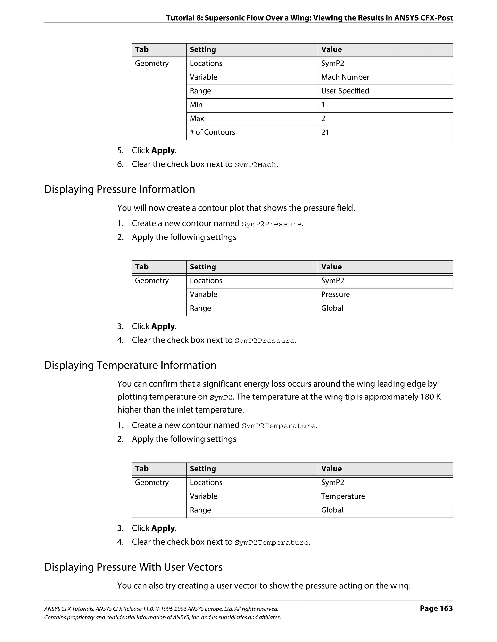
![Tutorial 8: Supersonic Flow Over a Wing: Viewing the Results in ANSYS CFX-Post
1. Create a new variable named Variable 1.
2. Apply the following settings
Name Setting Value
Variable 1 Vector (Selected)
X Expression (Pressure+101325[Pa])*Normal X
Y Expression (Pressure+101325[Pa])*Normal Y
Z Expression (Pressure+101325[Pa])*Normal Z
3. Click Apply.
4. Create a new vector named Vector 1.
5. Apply the following settings
Tab Setting Value
Geometry Locations WingSurface
Variable Variable 1
Symbol Symbol Size 0.04
6. Click Apply.
7. Zoom in on the wing in order to see the created vector plot.
Page 164 ANSYS CFX Tutorials. ANSYS CFX Release 11.0. © 1996-2006 ANSYS Europe, Ltd. All rights reserved.
Contains proprietary and confidential information of ANSYS, Inc. and its subsidiaries and affiliates.](https://image.slidesharecdn.com/ansys11tutorial-111218135319-phpapp01/75/Ansys-11-tutorial-176-2048.jpg)
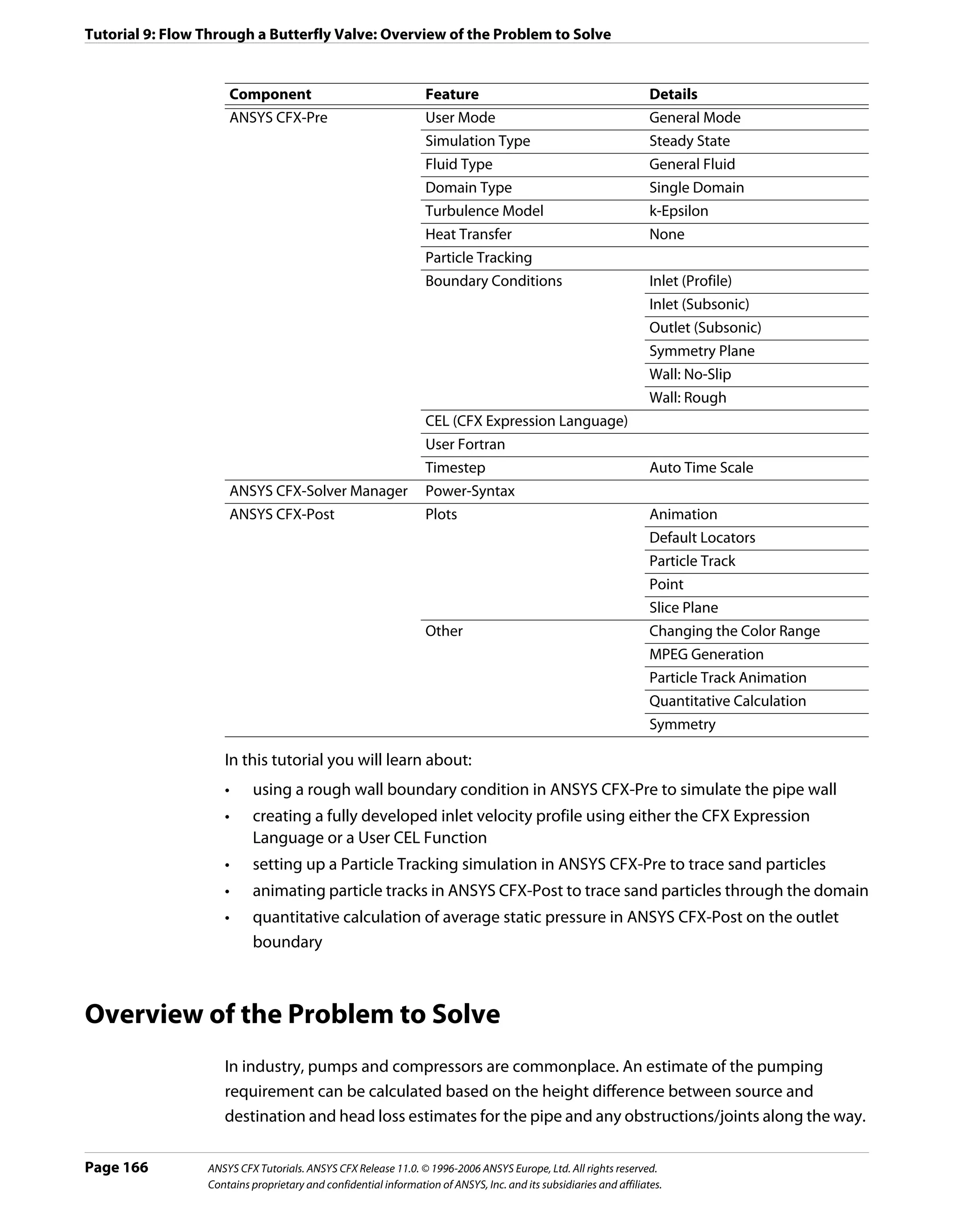


![Tutorial 9: Flow Through a Butterfly Valve: Defining a Simulation in ANSYS CFX-Pre
2. Apply the following settings:
Tab Setting Value
Basic Settings Material Group Particle Solids
Thermodynamic State (Selected)
Material Properties Thermodynamic Properties > Equation of 2300 [kg m^-3]
State > Density
Thermodynamic Properties >Specific Heat (Selected)
Capacity
Thermodynamic Properties >Specific Heat 0 [J kg^-1 K^-1]*
Capacity > Specific Heat Capacity
Thermodynamic Properties > Reference (Selected)
State
Thermodynamic Properties > Reference Specified Point
State > Option
Thermodynamic Properties > Reference 300 [K]
State > Ref. Temperature
*. This value is not used because heat transfer is not modeled in this tutorial.
3. Click OK.
4. Under Materials, right-click Sand Fully Coupled and select Duplicate from the
shortcut menu.
5. Name the duplicate Sand One Way Coupled.
6. Click OK.
Sand One Way Coupled is created with properties identical to Sand Fully Coupled.
Creating the Domain
1. Right click Simulation in the Outline tree view and ensure that Automatic Default
Domain is selected. A domain named Default Domain should now appear under the
Simulation branch.
2. Double click Default Domain and apply the following settings
Tab Setting Value
General Options Basic Settings > Fluids List Water
Basic Settings > Particle Tracking (Selected)
Basic Settings > Particle Tracking > Particles List Sand Fully Coupled,
Sand One Way Coupled
Domain Models > Pressure > Reference Pressure 1 [atm]
Fluid Models Heat Transfer > Option None
Turbulence > Option k-Epsilon*
ANSYS CFX Tutorials. ANSYS CFX Release 11.0. © 1996-2006 ANSYS Europe, Ltd. All rights reserved. Page 169
Contains proprietary and confidential information of ANSYS, Inc. and its subsidiaries and affiliates.](https://image.slidesharecdn.com/ansys11tutorial-111218135319-phpapp01/75/Ansys-11-tutorial-181-2048.jpg)
![Tutorial 9: Flow Through a Butterfly Valve: Defining a Simulation in ANSYS CFX-Pre
Tab Setting Value
Fluid Details Sand Fully Coupled (Selected)
Sand Fully Coupled > Morphology > Option Solid Particles
Sand Fully Coupled > Morphology > Particle (Selected)
Diameter Distribution
Sand Fully Coupled > Morphology > Particle Normal in Diameter by
Diameter Distribution > Option Mass
Sand Fully Coupled > Morphology > Particle 50e-6 [m]
Diameter Distribution > Minimum Diameter
Sand Fully Coupled > Morphology > Particle 500e-6 [m]
Diameter Distribution > Maximum Diameter
Sand Fully Coupled > Morphology > Particle 250e-6 [m]
Diameter Distribution > Mean Diameter
Sand Fully Coupled > Morphology > Particle 70e-6 [m]
Diameter Distribution > Std. Deviation
Sand Fully Coupled > Erosion Model (Selected)
Sand Fully Coupled > Erosion Model > Option Finnie
Sand Fully Coupled > Erosion Model > Vel. 2.0
Power Factor
Sand Fully Coupled > Erosion Model > Reference 1 [m s^-1]
Velocity
*. The turbulence model only applies to the continuous phase and not the particle
phases.
3. Apply the following settings
Page 170 ANSYS CFX Tutorials. ANSYS CFX Release 11.0. © 1996-2006 ANSYS Europe, Ltd. All rights reserved.
Contains proprietary and confidential information of ANSYS, Inc. and its subsidiaries and affiliates.](https://image.slidesharecdn.com/ansys11tutorial-111218135319-phpapp01/75/Ansys-11-tutorial-182-2048.jpg)
![Tutorial 9: Flow Through a Butterfly Valve: Defining a Simulation in ANSYS CFX-Pre
Tab Setting Value
Fluid Details Sand One Way Coupled (Selected)
Sand One Way Coupled > Morphology > Solid Particles
Option
Sand One Way Coupled > Morphology > (Selected)
Particle Diameter Distribution
Sand One Way Coupled > Morphology > Normal in Diameter by Mass
Particle Diameter Distribution > Option
Sand One Way Coupled > Morphology > 50e-6 [m]
Particle Diameter Distribution > Minimum
Diameter
Sand One Way Coupled > Morphology > 500e-6 [m]
Particle Diameter Distribution > Maximum
Diameter
Sand One Way Coupled > Morphology > 250e-6 [m]
Particle Diameter Distribution > Mean
Diameter
Sand One Way Coupled > Morphology > 70e-6 [m]
Particle Diameter Distribution > Std.
Deviation
Sand One Way Coupled > Erosion Model (Selected)
Sand One Way Coupled > Erosion Model > Finnie
Option
Sand One Way Coupled > Erosion Model > 2.0
Vel. Power Factor
Sand One Way Coupled > Erosion Model > 1 [m s^-1]
Reference Velocity
4. Apply the following settings
Tab Setting Value
Fluid Details Water (Selected)
Water > Morphology > Option Continuous Fluid
Fluid Pairs Fluid Pairs Water | Sand Fully
Coupled
Fluid Pairs > Water | Sand Fully Coupled > Fully Coupled
Particle Coupling
Fluid Pairs > Water | Sand Fully Coupled > Schiller Naumann
Momentum Transfer > Drag Force > Option
Fluid Pairs Water | Sand One Way
Coupled
Fluid Pairs > Water | Sand One Way Coupled > One-way Coupling
Particle Coupling
Fluid Pairs > Water | Sand One Way Coupled > Schiller Naumann
Momentum Transfer > Drag Force > Option
5. Click OK.
ANSYS CFX Tutorials. ANSYS CFX Release 11.0. © 1996-2006 ANSYS Europe, Ltd. All rights reserved. Page 171
Contains proprietary and confidential information of ANSYS, Inc. and its subsidiaries and affiliates.](https://image.slidesharecdn.com/ansys11tutorial-111218135319-phpapp01/75/Ansys-11-tutorial-183-2048.jpg)
![Tutorial 9: Flow Through a Butterfly Valve: Defining a Simulation in ANSYS CFX-Pre
Creating the Inlet Velocity Profile
In previous tutorials you have often defined a uniform velocity profile at an inlet boundary.
This means that the inlet velocity near to the walls is the same as that at the center of the
inlet. If you look at the results from these simulations, you will see that downstream of the
inlet, a boundary layer will develop, so that the downstream near wall velocity is much lower
than the inlet near wall velocity.
You can simulate an inlet more accurately by defining an inlet velocity profile, so that the
boundary layer is already fully developed at the inlet. The one seventh power law will be
used in this tutorial to describe the profile at the pipe inlet. The equation for this is:
1
--
r 7
U = W max ⎛ 1 – ---------- ⎞
- (Eqn. 1)
⎝ R max⎠
where W max is the pipe centerline velocity, R max is the pipe radius, and r is the distance
from the pipe centerline.
A non uniform (profile) boundary condition can be created by:
• Creating an expression using CEL that describes the inlet profile.
OR
• Creating a User CEL Function which uses a user subroutine (linked to the ANSYS
CFX-Solver during execution) to describe the inlet profile.
OR
• Loading a BC profile file (a file which contains profile data).
Profiles created from data files are not used in this tutorial, but are used in the tutorial
Tutorial 3: Flow in a Process Injection Mixing Pipe (p. 77).
In this tutorial, you use one of the first two methods listed above to define the velocity
profile for the inlet boundary condition. The results from each method will be identical.
Using a CEL expression is the easiest way to create the profile. The User CEL Function
method is more complex but is provided as an example of how to use this feature. For more
complex profiles, it may be necessary to use a User CEL Function or a BC profile file.
To use the User CEL Function method, continue with this tutorial from User CEL Function
Method for the Inlet Velocity Profile (p. 173). Note that you will need access to a Fortran
compiler to be able to complete the tutorial by the User CEL Function method.
To use the expression method, continue with the tutorial from this point.
Expression 1. Create the following expressions.
Method for the
Inlet Velocity
Profile Name Definition
Rmax 20 [mm]
Wmax 5 [m s^-1]
Wprof Wmax*(abs(1-r/Rmax)^0.143)
Page 172 ANSYS CFX Tutorials. ANSYS CFX Release 11.0. © 1996-2006 ANSYS Europe, Ltd. All rights reserved.
Contains proprietary and confidential information of ANSYS, Inc. and its subsidiaries and affiliates.](https://image.slidesharecdn.com/ansys11tutorial-111218135319-phpapp01/75/Ansys-11-tutorial-184-2048.jpg)
![Tutorial 9: Flow Through a Butterfly Valve: Defining a Simulation in ANSYS CFX-Pre
The output produced when this command is executed will be printed to your terminal
window.
Note: You can use the -double option (that is, cfx5mkext -double PipeValve_inlet.F)
to compile the subroutine for use with double precision.
A subdirectory will have been created in your working directory whose name is system
dependent (for example, on IRIX it is named irix). This subdirectory contains the
shared object library.
Note: If you are running problems in parallel over multiple platforms then you will need to
create these subdirectories using the cfx5mkext command for each different platform.
• You can view more details about the cfx5mkext command by running
cfx5mkext -help
• You can set a Library Name and Library Path using the -name and -dest options
respectively.
• If these are not specified, the default Library Name is that of your Fortran file and the
default Library Path is your current working directory.
6. Close the Command Editor dialog box.
Creating the Input Arguments
Next, you will create some values that will be used as input arguments when the subroutine
is called.
1. Click Expression .
2. Set Name to Wmax, and then click OK.
3. Type 5 [m s^-1] into the Definition box, and then click Apply.
The expression will be listed in the Expressions tree view.
4. Use the same method to create an expression named Rmax defined to be 20 [mm].
Creating the User CEL Function
Two steps are required to define a User CEL Function that uses the compiled Fortran
subroutine. First, a User Routine that points to the Fortran subroutine will be created. Then
a User CEL Function that points to the User Routine will be created.
1. From the main toolbar, click User Routine .
2. Set Name to WprofRoutine, and then click OK.
The User Routine details view appears.
3. Set Option to User CEL Function.
4. Set Calling Name to inlet_velocity.
• This is the name of the subroutine within the Fortran file.
• Always use lower case letters for the calling name, even if the subroutine name in
the Fortran file is in upper case.
5. Set Library Name to PipeValve_inlet.
• This is the name passed to the cfx5mkext command by the -name option.
• If the -name option is not specified, a default is used.
Page 174 ANSYS CFX Tutorials. ANSYS CFX Release 11.0. © 1996-2006 ANSYS Europe, Ltd. All rights reserved.
Contains proprietary and confidential information of ANSYS, Inc. and its subsidiaries and affiliates.](https://image.slidesharecdn.com/ansys11tutorial-111218135319-phpapp01/75/Ansys-11-tutorial-186-2048.jpg)
![Tutorial 9: Flow Through a Butterfly Valve: Defining a Simulation in ANSYS CFX-Pre
• The default is the Fortran file name without the .F extension.
6. Set Library Path to the directory where the cfx5mkext command was executed
(usually the current working directory). For example:
• UNIX: /home/user/cfx/tutorials/PipeValve.
• Windows: c:usercfxtutorialsPipeValve.
This can be accomplished quickly by clicking Browse (next to Library Path),
browsing to the appropriate folder in Select Directory (not necessary if selecting
the working directory), and clicking OK (in Select Directory).
7. Click OK to complete the definition of the user routine.
8. Click User Function .
9. Set Name to WprofFunction, and then click OK.
The Function details view appears.
Important: You must not use the same name for the function and the routine.
10. Set Option to User Function.
11. Set User Routine Name to WprofRoutine.
12. Set Argument Units to [m s^-1], [m], [m]. These are the units for the three input
arguments: Wmax, r, and Rmax.
Set Result Units to [m s^-1], since the result will be a velocity for the inlet.
1. Click OK to complete the User Function specification.
You can now use the user function (WprofFunction) in place of a velocity value by
entering the expression WprofFunction(Wmax, r, Rmax) (although it only makes
sense for the W component of the inlet velocity in this tutorial).
In the definition of WprofFunction, the variable r (radius) is a system variable defined
as:
2 2
r = x +y (Eqn. 3)
In this equation, x and y are defined as directions 1 and 2 (X and Y for Cartesian
coordinate frames) respectively, in the selected reference coordinate frame.
Creating the Boundary Conditions
Inlet Boundary 1. Create a new boundary condition named inlet.
2. Apply the following settings
Tab Setting Value
Basic Settings Boundary Type Inlet
Location inlet
ANSYS CFX Tutorials. ANSYS CFX Release 11.0. © 1996-2006 ANSYS Europe, Ltd. All rights reserved. Page 175
Contains proprietary and confidential information of ANSYS, Inc. and its subsidiaries and affiliates.](https://image.slidesharecdn.com/ansys11tutorial-111218135319-phpapp01/75/Ansys-11-tutorial-187-2048.jpg)
![Tutorial 9: Flow Through a Butterfly Valve: Defining a Simulation in ANSYS CFX-Pre
Tab Setting Value
Boundary Mass And Momentum > Option Cart. Vel. Components
Details Mass And Momentum > U 0 [m s^-1]
Mass And Momentum > V 0 [m s^-1]
Mass And Momentum > W Wprof -OR-
WprofFunction(Wmax,
r, Rmax)*
Fluid Values† Boundary Conditions Sand Fully Coupled
Sand Fully Coupled > Particle Behavior > Define (Selected)
Particle Behavior
Sand Fully Coupled > Mass and Momentum > Cart. Vel. Components‡
Option
Sand Fully Coupled > Mass And Momentum > U 0 [m s^-1]
Sand Fully Coupled > Mass And Momentum > V 0 [m s^-1]
Sand Fully Coupled > Mass And Momentum > W Wprof -OR-
WprofFunction(Wmax,
r, Rmax)**
Sand Fully Coupled > Particle Position > Option Uniform Injection
Sand Fully Coupled > Particle Position > Number Direct Specification
of Positions > Option
Sand Fully Coupled > Particle Position > Number 200
of Positions > Number
Sand Fully Coupled > Particle Mass Flow > Mass 0.01 [kg s^-1]
Flow Rate
Fluid Values Boundary Conditions Sand One Way Coupled
Sand One Way Coupled > Particle Behavior > (Selected)
Define Particle Behavior
Sand One Way Coupled > Mass and Momentum > Cart. Vel. Components††
Option
Sand One Way Coupled > Mass And Momentum > 0 [m s^-1]
U
Sand One Way Coupled > Mass And Momentum > 0 [m s^-1]
V
Sand One Way Coupled > Mass And Momentum > Wprof -OR-
W WprofFunction(Wmax,
r, Rmax)‡‡
Sand One Way Coupled > Particle Position > Uniform Injection
Option
Sand One Way Coupled > Particle Position > Direct Specification
Number of Positions > Option
Sand One Way Coupled > Particle Position > 5000
Number of Positions > Number
Sand One Way Coupled > Particle Position > 0.01 [kg s^-1]
Particle Mass Flow Rate > Mass Flow Rate
Page 176 ANSYS CFX Tutorials. ANSYS CFX Release 11.0. © 1996-2006 ANSYS Europe, Ltd. All rights reserved.
Contains proprietary and confidential information of ANSYS, Inc. and its subsidiaries and affiliates.](https://image.slidesharecdn.com/ansys11tutorial-111218135319-phpapp01/75/Ansys-11-tutorial-188-2048.jpg)
![Tutorial 9: Flow Through a Butterfly Valve: Defining a Simulation in ANSYS CFX-Pre
*. Use the Expressions details view to enter either Wprof if using the expression
method, or WprofFunction(Wmax, r, Rmax) if using the User CEL Function
method.
†. Do NOT select Particle Diameter Distribution. The diameter distribution was
defined when creating the domain; this option would override those settings for
this boundary only.
‡. Instead of manually specifying the same velocity profile as the fluid, you can also
select the Zero Slip Velocity option.
**. as you did on the Boundary Details tab
††. Instead of manually specifying the same velocity profile as the fluid, you can also
select the Zero Slip Velocity option.
‡‡. as you did on the Boundary Details tab
3. Click OK.
One-way coupled particles are tracked as a function of the fluid flow field. The latter is not
influenced by the one-way coupled particles. The fluid flow will therefore be influenced by
the 0.01 [kg s^-1] flow of two-way coupled particles, but not by the 0.01 [kg s^-1] flow of
one-way coupled particles.
Outlet 1. Create a new boundary condition named outlet.
Boundary 2. Apply the following settings
Tab Setting Value
Basic Settings Boundary Type Outlet
Location outlet
Boundary Flow Regime > Option Subsonic
Details Mass and Momentum > Option Average Static Pressure
Mass and Momentum > Relative Pressure 0 [Pa]
3. Click OK.
Symmetry Plane 1. Create a new boundary condition named symP.
Boundary 2. Apply the following settings
Tab Setting Value
Basic Settings Boundary Type Symmetry
Location symP
3. Click OK.
Pipe Wall 1. Create a new boundary condition named pipe wall.
Boundary 2. Apply the following settings
Tab Setting Value
Basic Boundary Type Wall
Settings
Location pipe wall
ANSYS CFX Tutorials. ANSYS CFX Release 11.0. © 1996-2006 ANSYS Europe, Ltd. All rights reserved. Page 177
Contains proprietary and confidential information of ANSYS, Inc. and its subsidiaries and affiliates.](https://image.slidesharecdn.com/ansys11tutorial-111218135319-phpapp01/75/Ansys-11-tutorial-189-2048.jpg)
![Tutorial 9: Flow Through a Butterfly Valve: Defining a Simulation in ANSYS CFX-Pre
Tab Setting Value
Boundary Wall Roughness > Option Rough Wall
Details Roughness Height 0.2 [mm]*
Fluid Boundary Conditions Sand Fully Coupled
Values Boundary Conditions > Sand Fully Coupled > Velocity Restitution Coefficient
> Option
Boundary Conditions > Sand Fully Coupled > Velocity 0.8
> Perpendicular Coeff.
Boundary Conditions > Sand Fully Coupled > Velocity 1
> Parallel Coeff.
Boundary Conditions Sand One Way Coupled
Boundary Conditions > Sand One Way Coupled > Restitution Coefficient
Velocity > Option
Boundary Conditions > Sand One Way Coupled > 0.8
Velocity > Perpendicular Coeff.
Boundary Conditions > Sand One Way Coupled > 1
Velocity > Parallel Coeff.
*. Make sure that you change the units to millimetres. The thickness of the first
element should be of the same order as the roughness height.
3. Click OK.
Editing the 1. In the Outline tree view, edit the boundary condition named Default Domain
Default Default.
Boundary 2. Apply the following settings
Condition
Tab Setting Value
Fluid Values Boundary Conditions Sand Fully Coupled
Boundary Conditions > Sand Fully 0.9
Coupled > Velocity > Perpendicular Coeff.
Boundary Conditions Sand One Way Coupled
Boundary Conditions > Sand One Way 0.9
Coupled > Velocity > Perpendicular Coeff.
3. Click OK.
Setting Initial Values
1. Click Global Initialization .
2. Apply the following settings
Page 178 ANSYS CFX Tutorials. ANSYS CFX Release 11.0. © 1996-2006 ANSYS Europe, Ltd. All rights reserved.
Contains proprietary and confidential information of ANSYS, Inc. and its subsidiaries and affiliates.](https://image.slidesharecdn.com/ansys11tutorial-111218135319-phpapp01/75/Ansys-11-tutorial-190-2048.jpg)
![Tutorial 9: Flow Through a Butterfly Valve: Defining a Simulation in ANSYS CFX-Pre
Tab Setting Value
Global Settings Initial Conditions > Cartesian Velocity Automatic with Value
Components > Option
Initial Conditions > Cartesian Velocity 0 [m s^-1]
Components > Option > U
Initial Conditions > Cartesian Velocity 0 [m s^-1]
Components > Option > V
Initial Conditions > Cartesian Velocity Wprof -OR-
Components > Option > W WprofFunction(Wmax, r,
Rmax)*
Initial Conditions > Turbulence Eddy (Selected)
Dissipation
*. Use Enter Expression to enter Wprof if using the Expression method; enter
WprofFunction(Wmax, r, Rmax) if using the User CEL Function method.
3. Click OK.
Setting Solver Control
1. Click Solver Control .
2. Apply the following settings
Tab Setting Value
Basic Settings Advection Scheme > Option Specified Blend Factor
Advection Scheme > Blend Factor 0.75
Particle Control Particle Integration > Maximum Tracking Time (Selected)
Particle Integration > Maximum Tracking Time 10 [s]
> Value
Particle Integration > Maximum Tracking (Selected)
Distance
Particle Integration > Maximum Tracking 10 [m]
Distance > Value
Particle Integration > Max. Num. Integration (Selected)
Steps
Particle Integration > Max. Num. Integration 10000
Steps > Value
Particle Integration > Max. Particle Intg. Time (Selected)
Step
Particle Integration > Max. Particle Intg. Time 1e+10 [s]
Step > Value
3. Click OK.
ANSYS CFX Tutorials. ANSYS CFX Release 11.0. © 1996-2006 ANSYS Europe, Ltd. All rights reserved. Page 179
Contains proprietary and confidential information of ANSYS, Inc. and its subsidiaries and affiliates.](https://image.slidesharecdn.com/ansys11tutorial-111218135319-phpapp01/75/Ansys-11-tutorial-191-2048.jpg)
![Tutorial 9: Flow Through a Butterfly Valve: Viewing the Results in ANSYS CFX-Post
Tab Setting Value
Color Mode Variable
Variable Sand One Way Coupled.Erosion Rate Density*
Range User Specified
Min 0 [kg m^-2 s^-1]
Max 25 [kg m^-2 s^-1]†
*. This is statistically better than Sand Fully Coupled.Erosion Rate Density since
many more particles were calculated for Sand One Way Coupled.
†. This range is used to gain a better resolution of the wall shear stress values around
the edge of the valve surfaces.
3. Click Apply.
As can be seen, the highest values occur on the edges of the valve where most particles
strike. Erosion of the low Z side of the valve would occur more quickly than for the high
Z side.
Particle Tracks
Default particle track objects are created at the start of the session. One particle track is
created for each set of particles in the simulation. You are going to make use of the default
object for Sand Fully Coupled.
The default object draws 10 tracks as lines from the inlet to outlet. Info shows information
about the total number of tracks, index range and the track numbers which are drawn.
1. Edit the object named Res PT for Sand Fully Coupled.
2. Apply the following settings
Tab Setting Value
Geometry Max Tracks 20
3. Click Apply.
Erosion on the Pipe Wall
The User Specified range for coloring will be set to resolve areas of stress on the pipe wall
near of the valve.
1. Clear the check box next to Res PT for Sand Fully Coupled.
2. Clear the check box next to Default Domain Default.
3. Edit the object named pipe wall.
4. Apply the following settings
ANSYS CFX Tutorials. ANSYS CFX Release 11.0. © 1996-2006 ANSYS Europe, Ltd. All rights reserved. Page 181
Contains proprietary and confidential information of ANSYS, Inc. and its subsidiaries and affiliates.](https://image.slidesharecdn.com/ansys11tutorial-111218135319-phpapp01/75/Ansys-11-tutorial-193-2048.jpg)
![Tutorial 9: Flow Through a Butterfly Valve: Viewing the Results in ANSYS CFX-Post
Tab Setting Value
Color Mode Variable
Variable Sand One Way Coupled.Erosion Rate Density
Range User Specified
Min 0 [kg m^-2 s^-1]
Max 25 [kg m^-2 s^-1]
5. Click Apply.
Particle Track Symbols
1. Clear visibility for all objects except Wireframe.
2. Edit the object named Res PT for Sand Fully Coupled.
3. Apply the following settings
Tab Setting Value
Color Mode Variable
Variable Sand Fully Coupled.Velocity w
Symbol Draw Symbols (Selected)
Draw Symbols > Max Time 0 [s]
Draw Symbols > Min Time 0 [s]
Draw Symbols > Interval 0.07 [s]
Draw Symbols > Symbol Fish3D
Draw Symbols > Symbol Size 0.5
4. Clear Draw Tracks.
5. Click Apply.
Symbols are placed at the start of each track.
Creating a Particle Track Animation
The following steps describe how to create a particle tracking animation using Quick
Animation. Similar effects can be achieved in more detail using the Keyframe Animation
option, which allows full control over all aspects on an animation.
1. Select Tools > Animation or click Animation .
2. Select Quick Animation.
3. Select Res PT for Sand Fully Coupled:
4. Click Options to display the Animation Options dialog box, then clear Override
Symbol Settings to ensure the symbol type and size are kept at their specified settings
for the animation playback. Click OK.
Note: The arrow pointing downward in the bottom right corner of the Animation Window
will reveal the Options button if it is not immediately visible.
Page 182 ANSYS CFX Tutorials. ANSYS CFX Release 11.0. © 1996-2006 ANSYS Europe, Ltd. All rights reserved.
Contains proprietary and confidential information of ANSYS, Inc. and its subsidiaries and affiliates.](https://image.slidesharecdn.com/ansys11tutorial-111218135319-phpapp01/75/Ansys-11-tutorial-194-2048.jpg)
![Tutorial 9: Flow Through a Butterfly Valve: Viewing the Results in ANSYS CFX-Post
5. Select Loop.
6. Deselect Repeat forever and ensure Repeat is set to 1.
7. Select Save MPEG.
8. Click Browse and enter tracks.mpg as the file name.
9. Click Play the animation .
10. If prompted to overwrite an existing movie, click Overwrite.
The animation plays and builds an .mpg file.
11. Close the Animation dialog box.
Performing Quantitative Calculations
On the outlet boundary condition you created in ANSYS CFX-Pre, you set the Average
Static Pressure to 0.0 [Pa]. To see the effect of this:
1. From the main menu select Tools > Function Calculator.
The Function Calculator is displayed. It allows you to perform a wide range of
quantitative calculations on your results.
Note: You should use Conservative variable values when performing calculations and
Hybrid values for visualization purposes. Conservative values are set by default in ANSYS
CFX-Post but you can manually change the setting for each variable in the Variables
Workspace, or the settings for all variables by using the Function Calculator.
2. Set Function to maxVal.
3. Set Location to outlet.
4. Set Variable to Pressure.
5. Click Calculate.
The result is the maximum value of pressure at the outlet.
6. Perform the calculation again using minVal to obtain the minimum pressure at the
outlet.
7. Select areaAve, and then click Calculate.
• This calculates the area weighted average of pressure.
• The average pressure is approximately zero, as specified by the boundary condition.
Other Features The geometry was created using a symmetry plane. You can display the other half of the
geometry by creating a YZ Plane at X = 0 and then editing the Default Transform object
to use this plane as a reflection plane.
1. When you have finished viewing the results, quit ANSYS CFX-Post.
ANSYS CFX Tutorials. ANSYS CFX Release 11.0. © 1996-2006 ANSYS Europe, Ltd. All rights reserved. Page 183
Contains proprietary and confidential information of ANSYS, Inc. and its subsidiaries and affiliates.](https://image.slidesharecdn.com/ansys11tutorial-111218135319-phpapp01/75/Ansys-11-tutorial-195-2048.jpg)

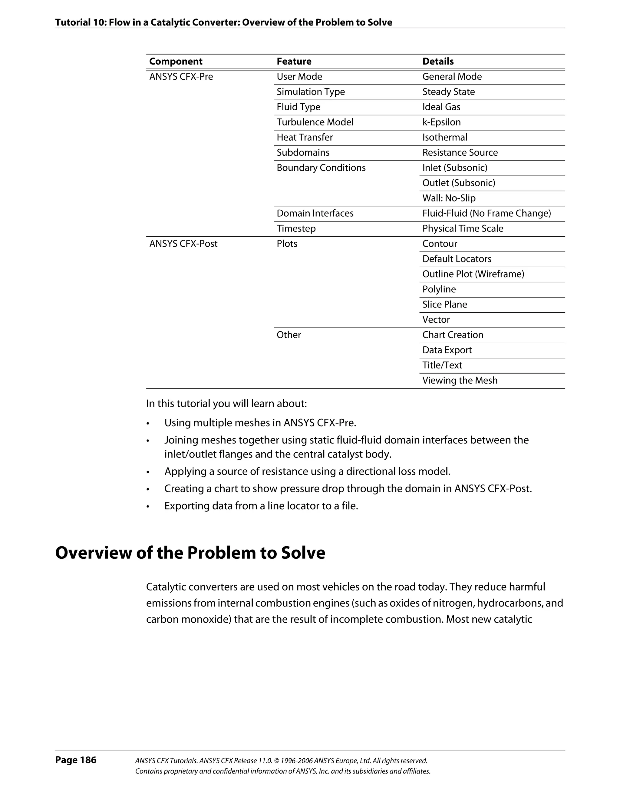
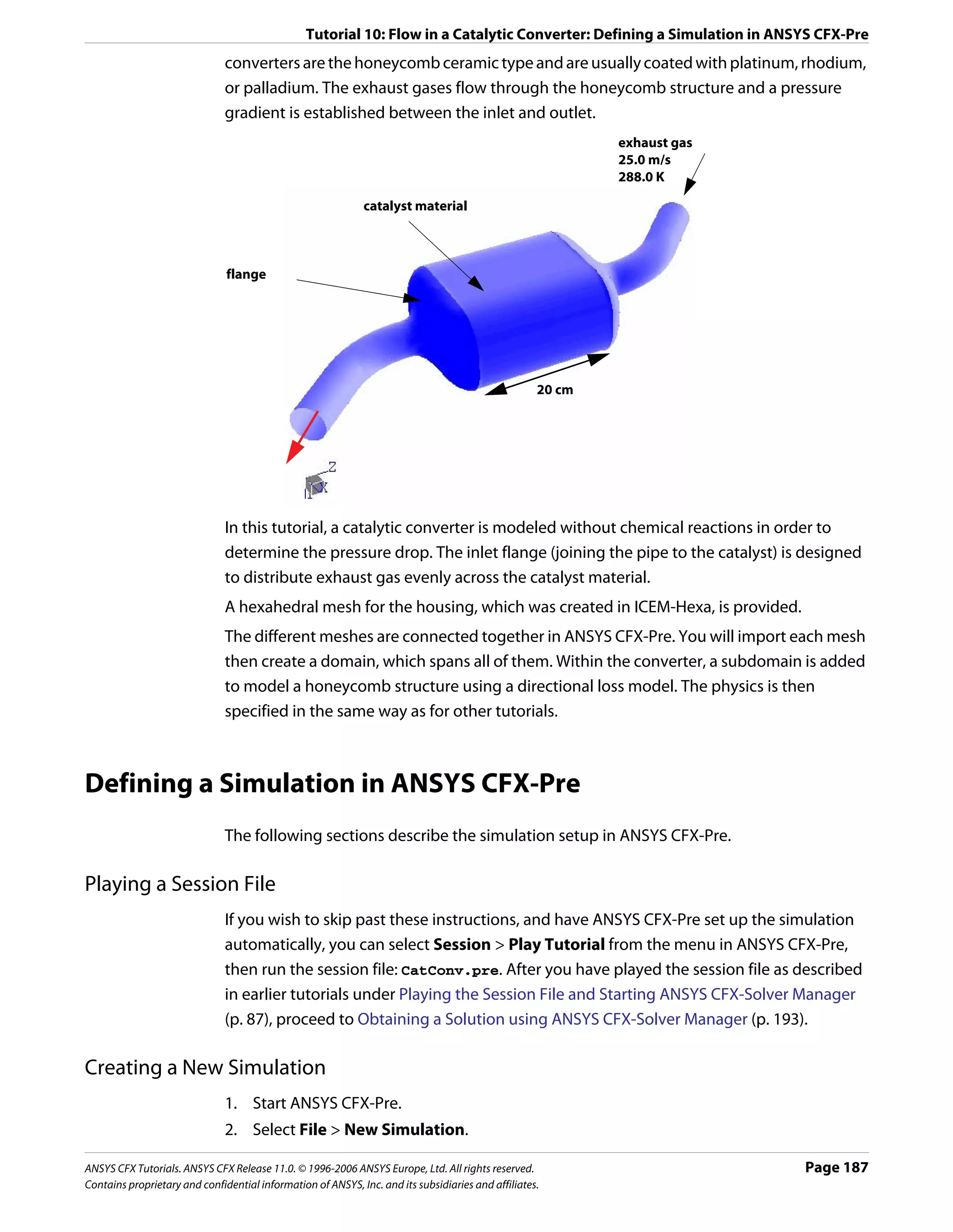

![Tutorial 10: Flow in a Catalytic Converter: Defining a Simulation in ANSYS CFX-Pre
Applying a Transform
The pipe and flange are located at the outlet end of the housing. The flange will be rotated
about an axis that points in the y-direction and is located at the center of the housing.
1. Right-click CatConvMesh.gtm and select Transform Mesh. The Mesh Transformation
Editor dialog box appears.
2. Apply the following settings
Tab Setting Value
Definition Apply Rotation > Rotation Option Rotation Axis
Apply Rotation > From 0, 0, 0.16
Apply Rotation > To 0, 1, 0.16*
Apply Rotation > Rotation Angle 180 [degree]
Multiple Copies (Selected)
Multiple Copies > # of Copies 1
*. This specifies an axis located at the center of the housing parallel to the y-axis.
3. Click OK.
Creating a Union Region
Three separate regions now exist, but since there is no relative motion between each region,
you only need to create a single domain. This can be done by simply using all three regions
in the domain Location list or, as in this case, by using the Region details view to create a
union of the three regions.
1. Create a new composite region named CatConverter.
2. Apply the following settings
Tab Setting Value
Basic Settings Dimension (Filter) 3D
Region List B1.P3, B1.P3 2, LIVE
3. Click OK.
Creating the Domain
For this simulation you will use an isothermal heat transfer model and assume turbulent
flow.
1. Click Domain and set the name to CatConv.
2. Apply the following settings
ANSYS CFX Tutorials. ANSYS CFX Release 11.0. © 1996-2006 ANSYS Europe, Ltd. All rights reserved. Page 189
Contains proprietary and confidential information of ANSYS, Inc. and its subsidiaries and affiliates.](https://image.slidesharecdn.com/ansys11tutorial-111218135319-phpapp01/75/Ansys-11-tutorial-201-2048.jpg)
![Tutorial 10: Flow in a Catalytic Converter: Defining a Simulation in ANSYS CFX-Pre
Tab Setting Value
General Basic Settings > Location CatConverter
Options
Basic Settings > Fluid List Air Ideal Gas
Domain Models > Pressure > Reference Pressure 1 [atm]
Fluid Models Heat Transfer > Option Isothermal
Heat Transfer > Fluid Temperature 600 [K]
3. Click OK.
Creating a Subdomain to Model the Catalyst Structure
The catalyst-coated honeycomb structure will be modeled using a subdomain with a
directional source of resistance.
For quadratic resistances, the pressure drop is modeled using:
∂p
------ = – K Q U U i
- (Eqn. 1)
∂x i
where K Q is the quadratic resistance coefficient, U i is the local velocity in the i direction,
∂p
and ------ is the pressure drop gradient in the i direction.
-
∂x i
1. Select Insert > Subdomain from the main menu or click Subdomain
2. In the Insert Subdomain dialog box, type catalyst.
3. Apply the following settings
Tab Setting Value
Basic Settings Location LIVE*
Sources† Sources (Selected)
Sources > Momentum Source/Porous Loss (Selected)
Sources > Momentum Source/Porous Loss > (Selected)
Directional Loss
*. This is the entire housing section.
†. Used to set sources of momentum, resistance and mass for the subdomain (Other
sources are available for different problem physics).
4. Apply the following settings in the Directional Loss section
Setting Value
Streamwise Direction > X Component 0
Streamwise Direction > Y Component 0
Streamwise Direction > Z Component 1
Page 190 ANSYS CFX Tutorials. ANSYS CFX Release 11.0. © 1996-2006 ANSYS Europe, Ltd. All rights reserved.
Contains proprietary and confidential information of ANSYS, Inc. and its subsidiaries and affiliates.](https://image.slidesharecdn.com/ansys11tutorial-111218135319-phpapp01/75/Ansys-11-tutorial-202-2048.jpg)
![Tutorial 10: Flow in a Catalytic Converter: Defining a Simulation in ANSYS CFX-Pre
Setting Value
Streamwise Loss > Option Linear and Quadratic
Coefs
Streamwise Loss > Quadratic Resistance Coefficient (Selected)
Streamwise Loss > Quadratic Resistance Coefficient > Quadratic 650 [kg m^-4]
Coefficient
5. Click OK.
Creating Boundary Conditions
Inlet Boundary 1. Create a new boundary condition named Inlet.
2. Apply the following settings
Tab Setting Value
Basic Settings Boundary Type Inlet
Location PipeEnd 2
Boundary Details Mass and Momentum > Normal Speed 25 [m s^-1]
3. Click OK.
Outlet 1. Create a new boundary condition named Outlet.
Boundary 2. Apply the following settings
Tab Setting Value
Basic Settings Boundary Type Outlet
Location PipeEnd
Boundary Details Mass and Momentum > Option Static Pressure
Mass and Momentum > Relative Pressure 0 [Pa]
3. Click OK.
The remaining surfaces are automatically grouped into the default no slip wall
boundary condition.
Creating the Domain Interfaces
Domain interfaces are used to define the connecting boundaries between meshes where
the faces do not match or when a frame change occurs. Meshes are ‘glued’ together using
the General Grid Interface (GGI) functionality of ANSYS CFX. Different types of GGI
connections can be made. In this case, you require a simple Fluid-Fluid Static connection (no
Frame Change). Other options allow you to change reference frame across the interface or
create a periodic boundary with dissimilar meshes on each periodic face.
Two Interfaces are required, one to connect the inlet flange to the catalyst housing and one
to connect the outlet flange to the catalyst housing.
ANSYS CFX Tutorials. ANSYS CFX Release 11.0. © 1996-2006 ANSYS Europe, Ltd. All rights reserved. Page 191
Contains proprietary and confidential information of ANSYS, Inc. and its subsidiaries and affiliates.](https://image.slidesharecdn.com/ansys11tutorial-111218135319-phpapp01/75/Ansys-11-tutorial-203-2048.jpg)
![Tutorial 10: Flow in a Catalytic Converter: Defining a Simulation in ANSYS CFX-Pre
Inlet Pipe / 1. Create a new domain interface named InletSide.
Housing 2. Apply the following settings
Interface
Tab Setting Value
Basic Settings Interface Side 1 > Region List FlangeEnd 2
Interface Side 2 > Region List INLET
3. Click OK.
Outlet Pipe / 1. Create a new domain interface named OutletSide.
Housing 2. Apply the following settings
Interface
Tab Setting Value
Basic Settings Interface Side 1 > Region List FlangeEnd
Interface Side 2 > Region List OUTLET
3. Click OK.
Setting Initial Values
A sensible guess for the initial velocity is to set it to the expected velocity through the
catalyst housing. As the inlet velocity is 25 [m s^-1] and the cross sectional area of the inlet
and housing are known, you can apply conservation of mass to obtain an approximate
velocity of 2 [m s^-1] through the housing.
1. Click Global Initialization .
2. Apply the following settings
Tab Setting Value
Global Initial Conditions > Cartesian Velocity Automatic with Value
Settings Components > Option
Initial Conditions > Cartesian Velocity 0 [m s^-1]
Components > U
Initial Conditions > Cartesian Velocity 0 [m s^-1]
Components > V
Initial Conditions > Cartesian Velocity -2 [m s^-1]
Components > W
Initial Conditions > Turbulence Eddy (Selected)
Dissipation
3. Click OK.
Setting Solver Control
Assuming velocities of 25 [m s^-1] in the inlet and outlet pipes, and 2 [m s^-1] in the catalyst
housing, an approximate fluid residence time of 0.1 [s] can be calculated. A sensible
timestep of 0.04 [s] (1/4 to 1/2 of the fluid residence time) will be applied.
Page 192 ANSYS CFX Tutorials. ANSYS CFX Release 11.0. © 1996-2006 ANSYS Europe, Ltd. All rights reserved.
Contains proprietary and confidential information of ANSYS, Inc. and its subsidiaries and affiliates.](https://image.slidesharecdn.com/ansys11tutorial-111218135319-phpapp01/75/Ansys-11-tutorial-204-2048.jpg)
![Tutorial 10: Flow in a Catalytic Converter: Obtaining a Solution using ANSYS CFX-Solver Manager
For the convergence criteria, an RMS value of at least 1e-05 is usually required for adequate
convergence, but the default value is sufficient for demonstration purposes.
1. Click Solver Control .
2. Apply the following settings
Tab Setting Value
Basic Settings Convergence Control > Fluid Timescale Physical Timescale
Control > Timescale Control
Convergence Control >Fluid Timescale 0.04 [s]
Control > Physical Timescale
3. Click OK.
Writing the Solver (.def) File
While writing the solver file, you will use the Summarize Interface Data option to display
information about the connection type used for each domain interface.
1. Click Write Solver File .
2. Apply the following settings
Setting Value
File name CatConv.def
Summarize Interface Data (Selected)
Quit CFX–Pre * (Selected)
*. If using ANSYS CFX-Pre in Standalone Mode.
3. Ensure Start Solver Manager is selected and click Save.
4. Once ANSYS CFX-Solver Manager launches, return to ANSYS CFX-Pre.
The Interface Summary dialog box is displayed. This displays information related to the
summary of interface connections.
5. Click OK.
6. If using Standalone Mode, quit ANSYS CFX-Pre, saving the simulation (.cfx) file at your
discretion.
Obtaining a Solution using ANSYS CFX-Solver Manager
When ANSYS CFX-Pre has shut down and the ANSYS CFX-Solver Manager has started, you
can obtain a solution to the CFD problem by following the instructions below:
1. Ensure Define Run is displayed.
2. Click Start Run.
ANSYS CFX-Solver runs and attempts to obtain a solution. This can take a long time
depending on your system. Eventually a dialog box is displayed.
ANSYS CFX Tutorials. ANSYS CFX Release 11.0. © 1996-2006 ANSYS Europe, Ltd. All rights reserved. Page 193
Contains proprietary and confidential information of ANSYS, Inc. and its subsidiaries and affiliates.](https://image.slidesharecdn.com/ansys11tutorial-111218135319-phpapp01/75/Ansys-11-tutorial-205-2048.jpg)


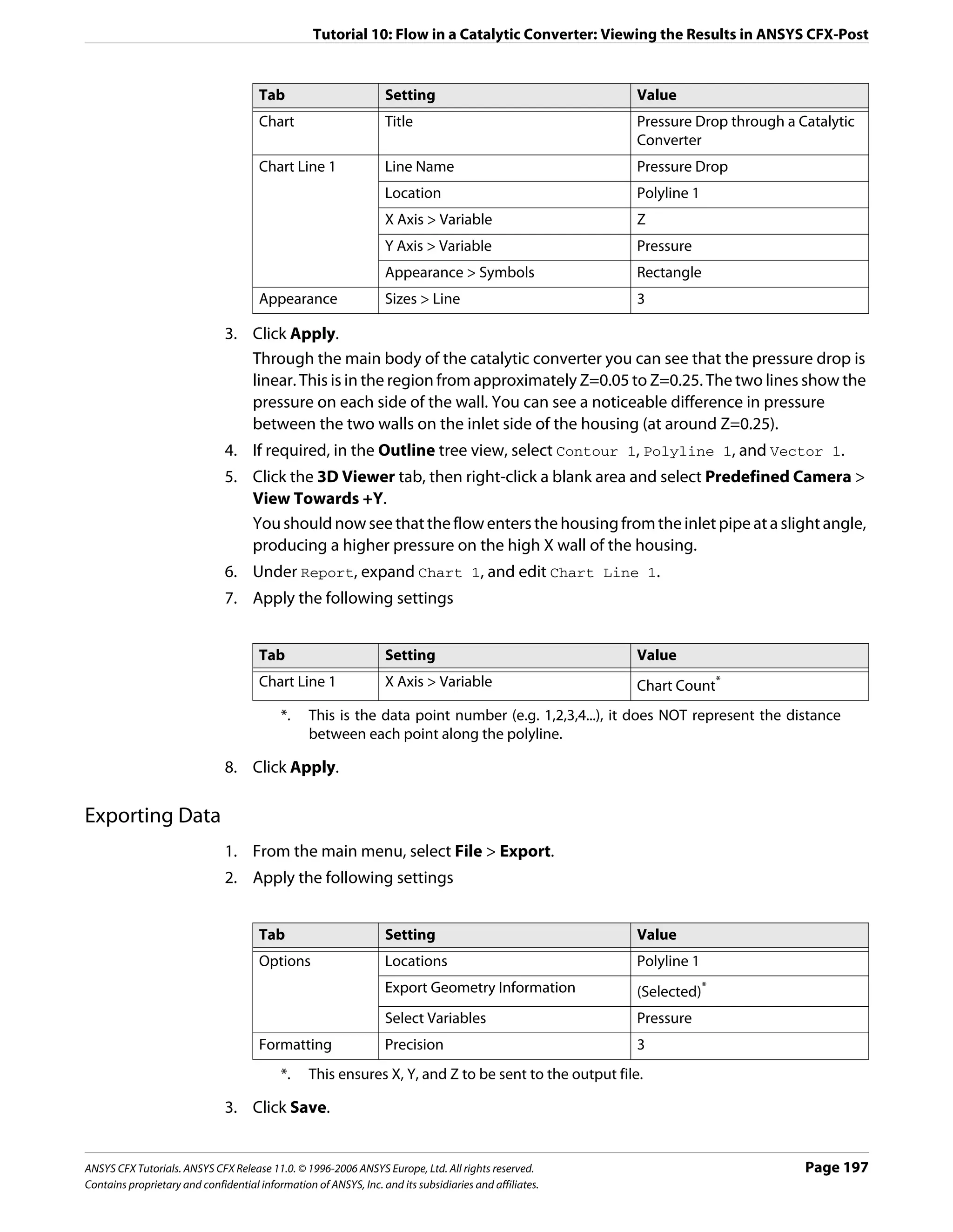


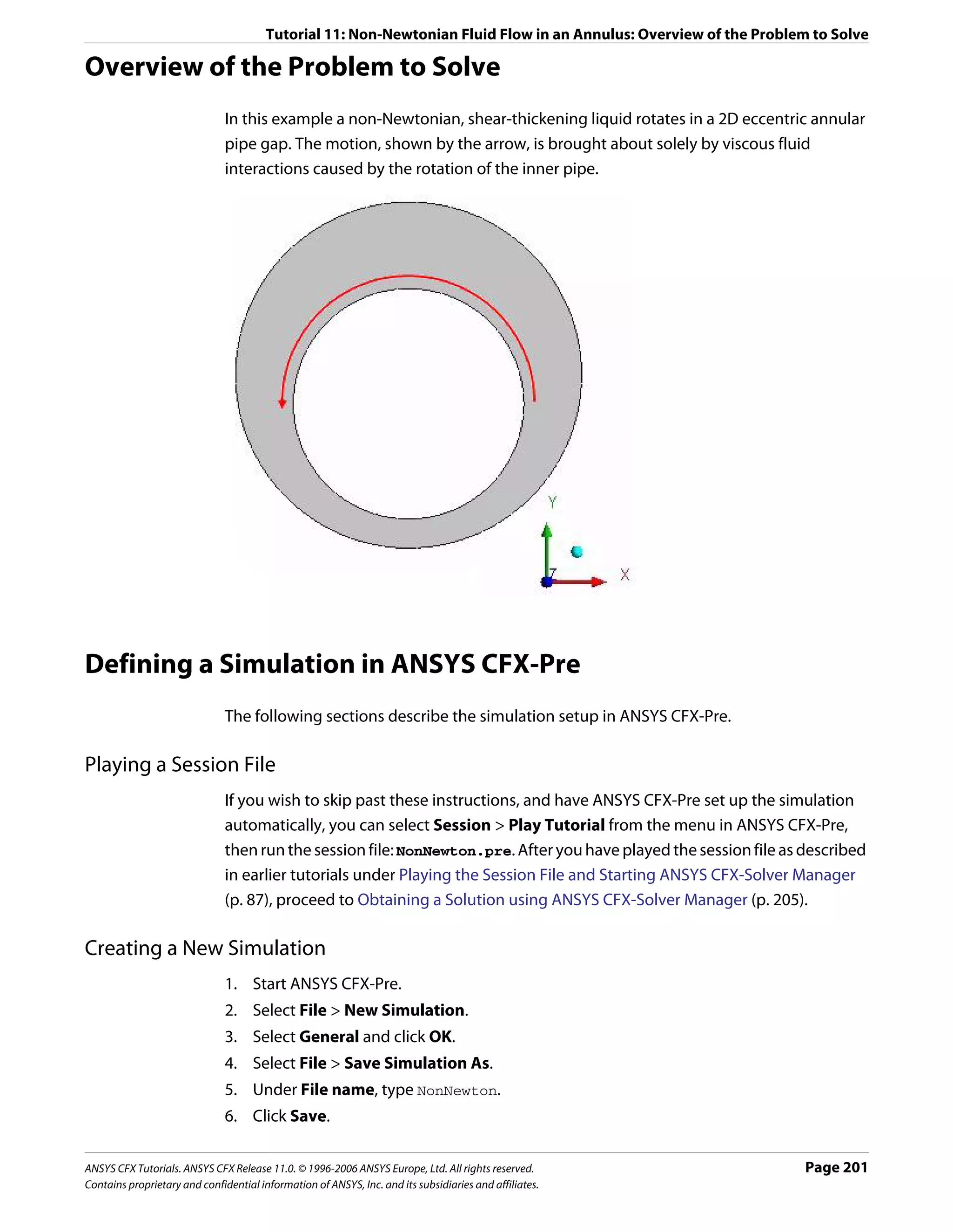
![Tutorial 11: Non-Newtonian Fluid Flow in an Annulus: Defining a Simulation in ANSYS CFX-Pre
Importing the Mesh
1. Right-click Mesh and select Import Mesh.
2. Apply the following settings
Setting Value
File name NonNewtonMesh.gtm
3. Click Open.
Creating an Expression for Shear Rate Dependent Viscosity
You can use an expression to define the dependency of fluid properties on other variables.
In this case, the fluid does not obey the simple linear Newtonian relationship between shear
stress and shear strain rate. The general relationship for the fluid you will model is given by:
n–1
µ = Kγ (Eqn. 1)
where γ is the shear strain rate and K and n are constants. For your fluid, n =1.5 and this
results in shear-thickening behavior of the fluid, i.e., the viscosity increases with increasing
shear strain rate. The shear strain rate is available as a ANSYS CFX-Pre System Variable
(sstrnr).
In order to describe this relationship using CEL, the dimensions must be consistent on both
sides of the equation. Clearly this means that K must have dimensions and requires units to
satisfy the equation. If the units of viscosity are kg m^-1 s^-1, and those of γ are s^-1, then
the expression is consistent if the units of K are kg m^-1 s^(-0.5).
1. Create the following expressions, remembering to click Apply after each is defined.
Name Definition
K 10.0 [kg m^-1 s^-0.5]
n 1.5
You should bound the viscosity to ensure that it remains physically meaningful. To do
so, you will create two additional parameters that will be used to guarantee the value of
the shear strain rate.
2. Create the following expressions for upper and lower bounds.
Name Definition
UpperS 100 [s^-1]
LowerS 1.0E-3 [s^-1]
ViscEqn K*(min(UpperS,max(sstrnr,LowerS))^(n-1))
3. Close the Expressions tab.
Page 202 ANSYS CFX Tutorials. ANSYS CFX Release 11.0. © 1996-2006 ANSYS Europe, Ltd. All rights reserved.
Contains proprietary and confidential information of ANSYS, Inc. and its subsidiaries and affiliates.](https://image.slidesharecdn.com/ansys11tutorial-111218135319-phpapp01/75/Ansys-11-tutorial-214-2048.jpg)
![Tutorial 11: Non-Newtonian Fluid Flow in an Annulus: Defining a Simulation in ANSYS CFX-Pre
Creating a New Fluid
1. Create a new material named myfluid.
2. Apply the following settings
Tab Setting Value
Basic Settings Thermodynamic State (Selected)
Material Properties Equation of State > Molar Mass 1 [kg kmol^-1]*
Equation of State > Density 1.0E+4 [kg m^-3]
Specific Heat Capacity (Selected)
Specific Heat Capacity > Specific Heat Capacity 0 [J kg^-1 K^-1]†
Reference State (Selected)
Reference State > Option Specified Point
Reference State > Ref. Temperature 25 [C]
Reference State > Reference Pressure 1 [atm]
Transport Properties > Dynamic Viscosity (Selected)
Transport Properties > Dynamic Viscosity > ViscEqn
Dynamic Viscosity
*. This is not the correct Molar Mass value, but this material property will not be used
by the ANSYS CFX-Solver for this case. In other cases it will be used.
†. This is not the correct value for specific heat, but this property will not be used in
the ANSYS CFX-Solver.
3. Click OK.
Creating the Domain
1. Click Domain and set the name to NonNewton.
2. Apply the following settings to NonNewton
Tab Setting Value
General Basic Settings > Fluids List myfluid
Options Domain Models > Pressure > Reference Pressure 1 [atm]
Fluid Models Heat Transfer > Option Isothermal
Heat Transfer > Fluid Temperature 25 C
Turbulence > Option None (Laminar)
3. Click OK.
Creating the Boundary Conditions
Wall Boundary 1. Create a new boundary condition named rotwall.
2. Apply the following settings
ANSYS CFX Tutorials. ANSYS CFX Release 11.0. © 1996-2006 ANSYS Europe, Ltd. All rights reserved. Page 203
Contains proprietary and confidential information of ANSYS, Inc. and its subsidiaries and affiliates.](https://image.slidesharecdn.com/ansys11tutorial-111218135319-phpapp01/75/Ansys-11-tutorial-215-2048.jpg)
![Tutorial 11: Non-Newtonian Fluid Flow in an Annulus: Defining a Simulation in ANSYS CFX-Pre
Tab Setting Value
Basic Settings Boundary Type Wall
Location rotwall
Boundary Details Wall Influence on Flow > Wall Velocity (Selected)
Wall Influence on Flow > Wall Velocity > Rotating Wall
Option
Wall Influence on Flow > Wall Velocity > 31.33 [rev min^-1]
Angular Velocity
3. Click OK.
Symmetry Plane 1. Create a new boundary condition named SymP1.
Boundary 2. Apply the following settings
Tab Setting Value
Basic Settings Boundary Type Symmetry
Location SymP1
3. Click OK.
4. Create a new boundary condition named SymP2.
5. Apply the following settings
Tab Setting Value
Basic Settings Boundary Type Symmetry
Location SymP2
6. Click OK.
The outer annulus surfaces will default to the no-slip stationary wall boundary
condition.
Setting Initial Values
A reasonable initial guess for the velocity field is a value of zero throughout the domain.
1. Click Global Initialization .
2. Apply the following settings
Tab Setting Value
Global Initial Conditions > Cartesian Velocity Components > Option Automatic with
Settings Value
Initial Conditions > Cartesian Velocity Components > U 0 [m s^-1]
Initial Conditions > Cartesian Velocity Components > V 0 [m s^-1]
Initial Conditions > Cartesian Velocity Components > W 0 [m s^-1]
3. Click OK.
Page 204 ANSYS CFX Tutorials. ANSYS CFX Release 11.0. © 1996-2006 ANSYS Europe, Ltd. All rights reserved.
Contains proprietary and confidential information of ANSYS, Inc. and its subsidiaries and affiliates.](https://image.slidesharecdn.com/ansys11tutorial-111218135319-phpapp01/75/Ansys-11-tutorial-216-2048.jpg)
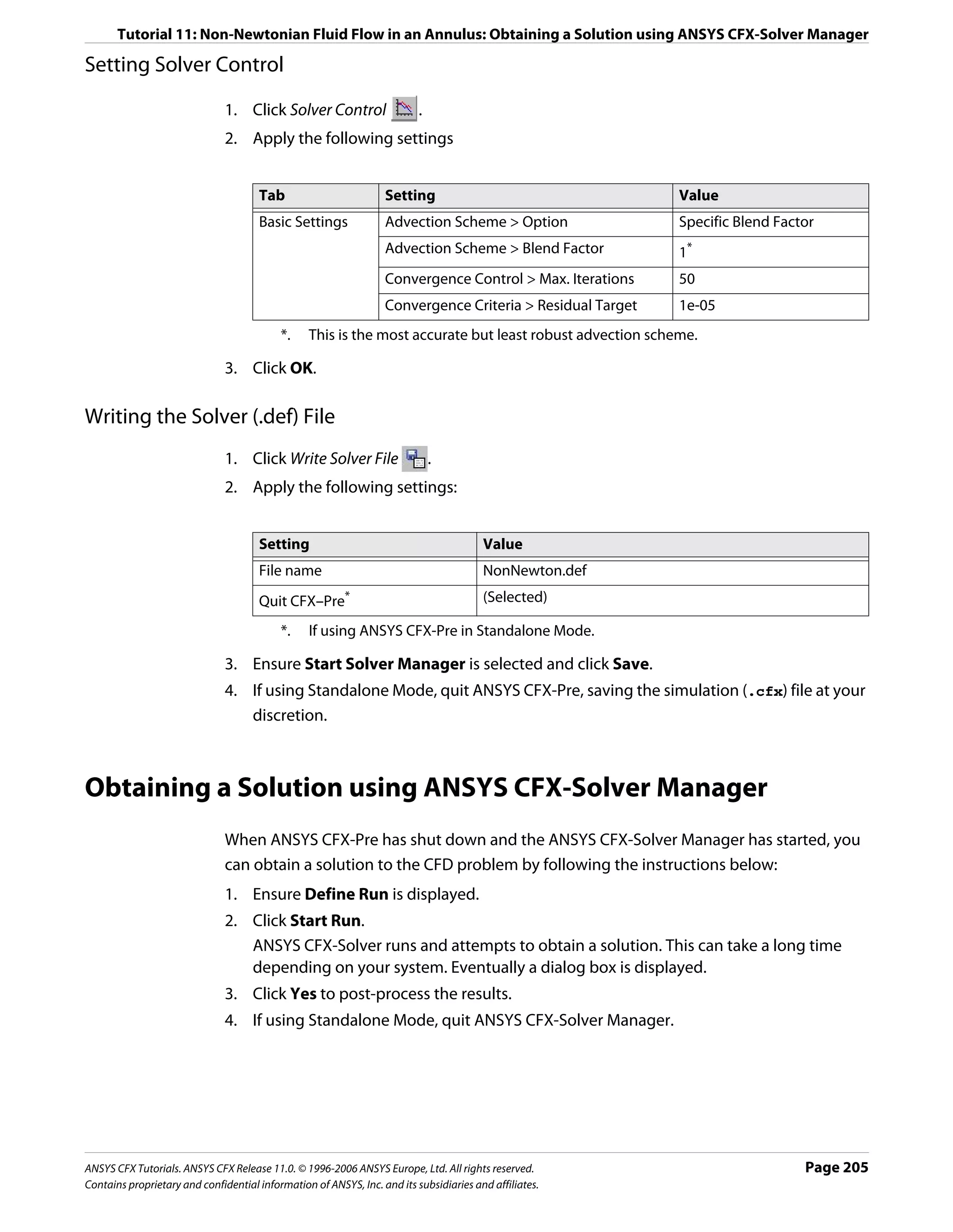
![Tutorial 11: Non-Newtonian Fluid Flow in an Annulus: Viewing the Results in ANSYS CFX-Post
Viewing the Results in ANSYS CFX-Post
In this tutorial you have used CEL to create an expression for the dynamic viscosity. If you
now perform calculations or color graphics objects using the Dynamic Viscosity variable, its
values will have been calculated from the expression you defined in ANSYS CFX-Pre.
These steps instruct the user on how to create a vector plot to show the velocity values in
the domain.
1. Right-click a blank area in the viewer and select Predefined Camera > View Towards
-Z from the shortcut menu.
2. Create a new plane named Plane 1.
3. Apply the following settings
Tab Setting Value
Geometry Definition > Method Point and Normal
Definition > Point 0, 0, 0.02
Definition > Normal 0, 0, 1
Plane Bounds > Type Circular
Plane Bounds > Radius 0.3 [m]
Plane Type Sample
Plane Type > R Samples 32
Plane Type > Theta Samples 24
Render Draw Faces (Cleared)
4. Click Apply.
5. Create a new vector plot named Vector 1.
6. Apply the following settings
Tab Setting Value
Geometry Definition > Locations Plane 1
Definition > Variable Velocity
Symbol Symbol Size 3
7. Click Apply.
8. Try creating some plots of your own, including one that shows the variation of dynamic
viscosity.
9. When you have finished, quit ANSYS CFX-Post.
Page 206 ANSYS CFX Tutorials. ANSYS CFX Release 11.0. © 1996-2006 ANSYS Europe, Ltd. All rights reserved.
Contains proprietary and confidential information of ANSYS, Inc. and its subsidiaries and affiliates.](https://image.slidesharecdn.com/ansys11tutorial-111218135319-phpapp01/75/Ansys-11-tutorial-218-2048.jpg)
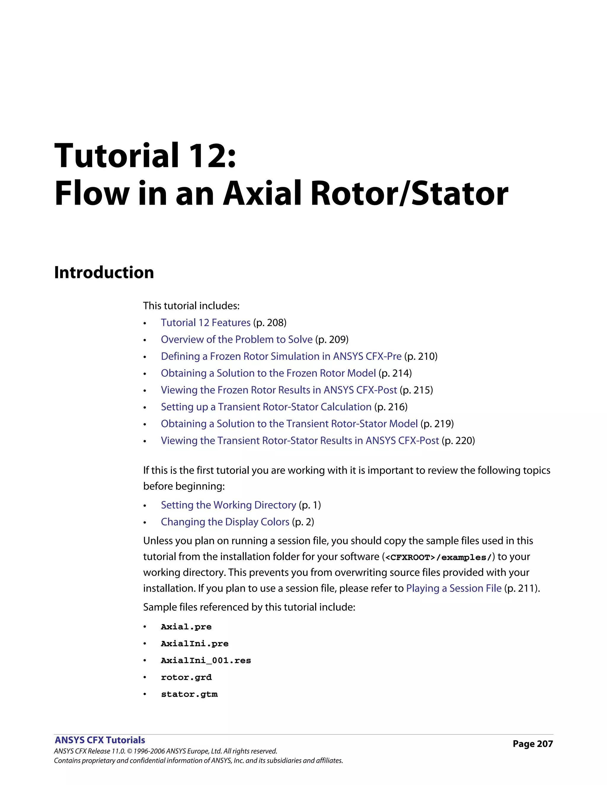
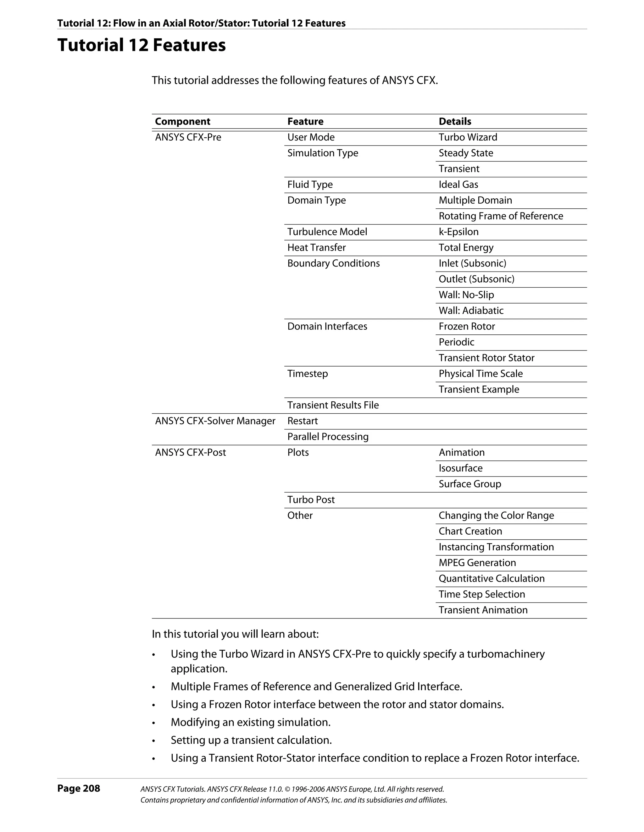

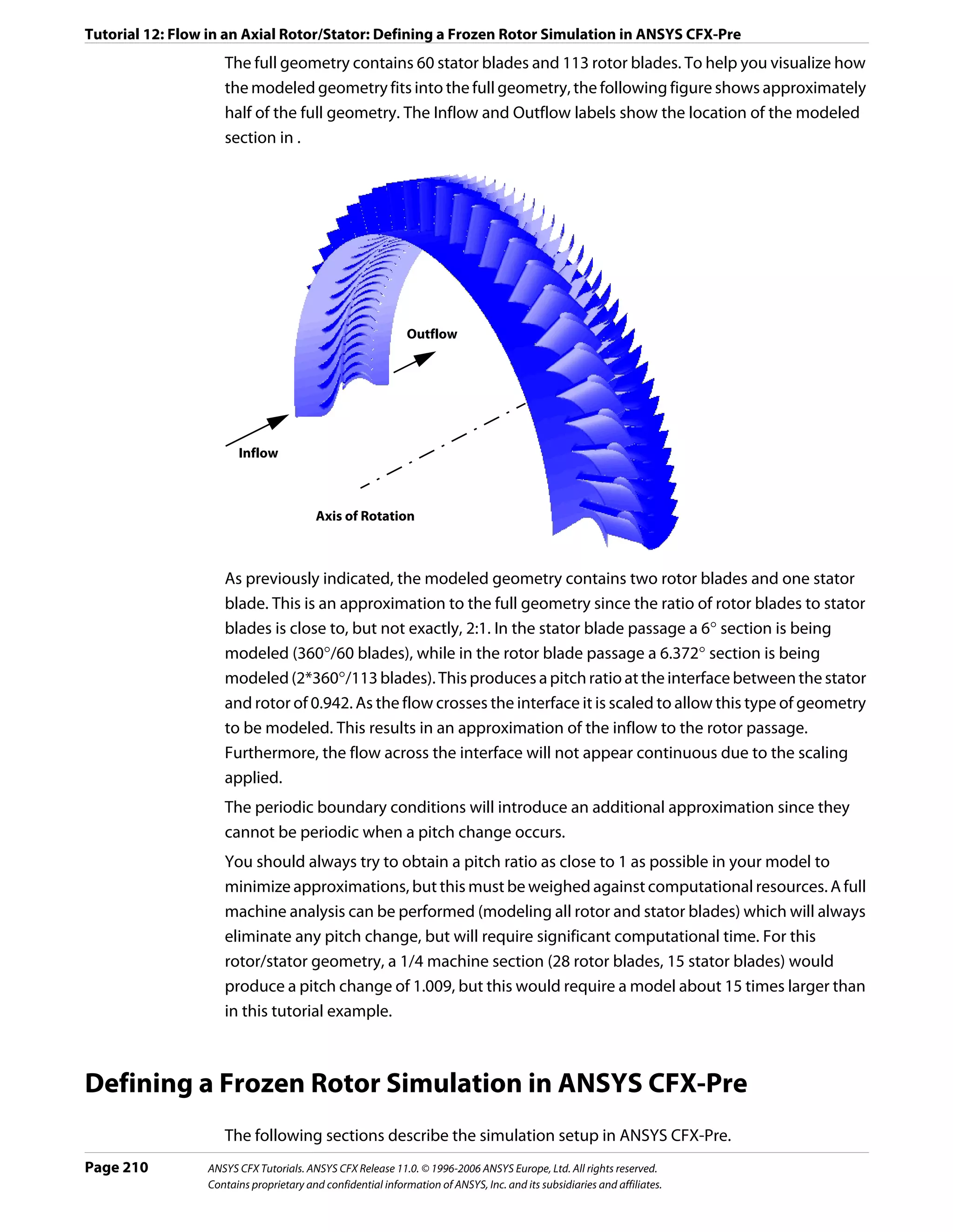

![Tutorial 12: Flow in an Axial Rotor/Stator: Defining a Frozen Rotor Simulation in ANSYS CFX-Pre
Setting Value
Component Type > Value 523.6 [radian s^-1]
Mesh File > File rotor.grd*
*. You may have to select the CFX-TASCflow option under File Type.
Note: The components must be ordered as above (stator then rotor) in order for the
interface to be created correctly. The order of the two components can be changed by right
clicking on S1 and selecting Move Component Up.
When a component is defined, Turbo Mode will automatically select a list of regions that
correspond to certain boundary condition types. This information should be reviewed
in the Region Information section to ensure that all is correct. This information will be
used to help set up boundary conditions and interfaces. The upper case turbo regions
that are selected (e.g., HUB) correspond to the region names in the CFX-TASCflow grd
file. CFX-TASCflow turbomachinery meshes use these names consistently.
6. Click Next.
Physics Definition
In this section, you will set properties of the fluid domain and some solver parameters.
1. Apply the following settings
Tab Setting Value
Physics Fluid Air Ideal Gas
Definition Simulation Type > Type Steady State
Model Data > Reference Pressure 0.25 [atm]
Model Data > Heat Transfer Total Energy
Model Data > Turbulence k-Epsilon
Boundary Templates > P-Total Inlet Mass Flow Outlet (Selected)
Boundary Templates > P-Total 0 [atm]
Boundary Templates > T-Total 340 [K]
Boundary Templates > Mass Flow Rate 0.06 [kg s^-1]
Interface > Default Type Frozen Rotor
Solver Parameters > Convergence Control Physical Timescale
Solver Parameters > Physical Timescale 0.002 [s]*
*. This time scale is approximately equal to 1 / ω , which is often appropriate for
rotating machinery applications.
2. Click Next.
Page 212 ANSYS CFX Tutorials. ANSYS CFX Release 11.0. © 1996-2006 ANSYS Europe, Ltd. All rights reserved.
Contains proprietary and confidential information of ANSYS, Inc. and its subsidiaries and affiliates.](https://image.slidesharecdn.com/ansys11tutorial-111218135319-phpapp01/75/Ansys-11-tutorial-224-2048.jpg)

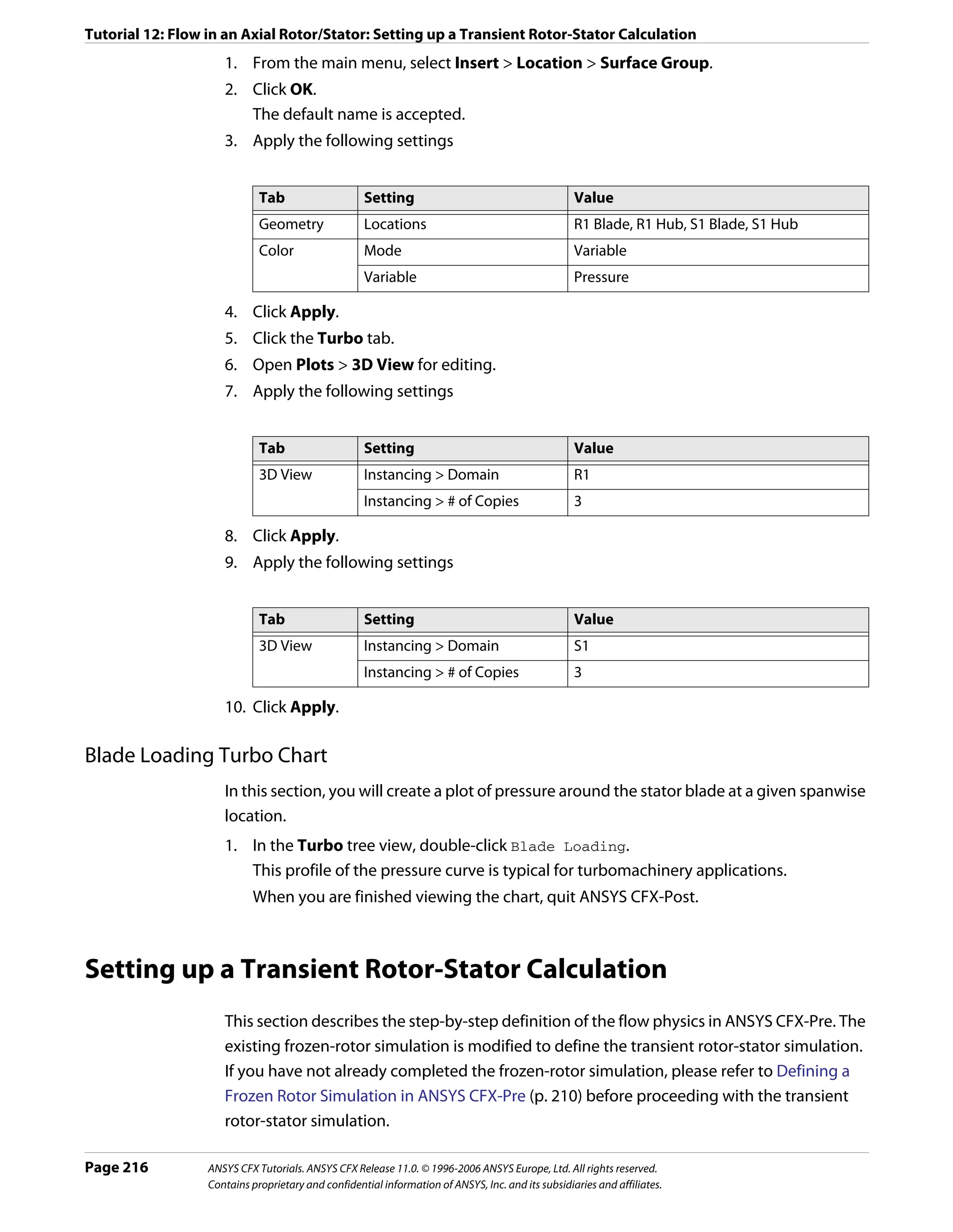
![Tutorial 12: Flow in an Axial Rotor/Stator: Setting up a Transient Rotor-Stator Calculation
Tab Setting Value
Physics Fluid Air Ideal Gas
Definition
Simulation Type > Type Transient
Simulation Type > Total Time 2.124e-4 [s]*
Simulation Type > Time Steps 2.124e-5 [s]†
Interface > Default Type Transient Rotor Stator
*. This gives 10 timesteps of 2.124e-5 s
†. This timestep will be used until the total time is reached
Note: A transient rotor-stator calculation often runs through more than one pitch. In these
cases, it may be useful to look at variable data averaged over the time interval required to
complete 1 pitch. You can then compare data for each pitch rotation to see if a “steady state”
has been achieved, or if the flow is still developing.
4. Click Next.
Interface Definition is displayed.
5. Click Next.
Boundary Definition is displayed.
6. Click Next.
Final Operations is displayed.
7. Ensure that Operation is set to Enter General Mode.
8. Click Finish.
Initial values are required, but will be supplied later using a results file.
Setting Output Control
1. Click Output Control .
2. Click the Trn Results tab.
3. Create a new transient result with the name Transient Results 1.
4. Apply the following settings to Transient Results 1
Setting Value
Option Selected Variables
Output Variables List * Pressure, Velocity, Velocity in Stn Frame
Output Frequency > Option Time Interval
Output Frequency > Time Interval 2.124e-5 [s]
*. Use the <Ctrl> key to select more than one variable.
5. Click OK.
Writing the Solver (.def) File
1. Click Write Solver File .
Page 218 ANSYS CFX Tutorials. ANSYS CFX Release 11.0. © 1996-2006 ANSYS Europe, Ltd. All rights reserved.
Contains proprietary and confidential information of ANSYS, Inc. and its subsidiaries and affiliates.](https://image.slidesharecdn.com/ansys11tutorial-111218135319-phpapp01/75/Ansys-11-tutorial-230-2048.jpg)
![Tutorial 12: Flow in an Axial Rotor/Stator: Viewing the Transient Rotor-Stator Results in ANSYS CFX-Post
2. Under the Color panel select Variable and set it to Pressure with a user specified range
of -10000 [Pa] to -7000 [Pa].
Setting up Instancing Transformations
Next, you will use instancing transformations to view a larger section of the model. The
properties for each domain have already been entered during the initialization phase, so
only the number of instances needs to be set.
1. In the Turbo tree view, double-click the 3D View object.
2. In the Instancing section of the form, set # of Copies to 6 for R1.
3. Click Apply.
4. In the Instancing section of the form, set # of Copies to 6 for S1.
5. Click Apply.
6. Return to the Outline tab and ensure that the turbo surface is visible again.
Creating a Transient Animation
Start by loading the first timestep:
1. Click Timestep Selector .
2. Select time value 0.
3. Click Apply to load the timestep.
The rotor blades move to their starting position. This is exactly 1 pitch from the previous
position so the blades will not appear to move.
4. Clear Visibility for Wireframe.
5. Position the geometry as shown below, ready for the animation. During the animation
the rotor blades will move to the right. Make sure you have at least two rotor blades out
of view to the left side of the viewer. They will come into view during the animation.
6. In the toolbar at the top of the window click Animation .
7. In the Animation dialog box, click New to create KeyFrameNo1.
8. Highlight KeyframeNo1, then set # of Frames to 9.
9. Use the Timestep Selector to load the final timestep.
ANSYS CFX Tutorials. ANSYS CFX Release 11.0. © 1996-2006 ANSYS Europe, Ltd. All rights reserved. Page 221
Contains proprietary and confidential information of ANSYS, Inc. and its subsidiaries and affiliates.](https://image.slidesharecdn.com/ansys11tutorial-111218135319-phpapp01/75/Ansys-11-tutorial-233-2048.jpg)


![Tutorial 13: Reacting Flow in a Mixing Tube: Defining a Simulation in ANSYS CFX-Pre
Tab Setting Value
Material Properties Thermodynamic Properties > Equation of State 19.52 [kg kmol^-1]*
> Molar Mass
Thermodynamic Properties > Equation of State 1080 [kg m^-3]
> Density
Thermodynamic Properties > Specific Heat (Selected)
Capacity
Thermodynamic Properties > Specific Heat 4190 [J kg^-1 K^-1]
Capacity > Specific Heat Capacity
Transport Properties > Dynamic Viscosity (Selected)
Transport Properties > Dynamic Viscosity > Value
Option
Transport Properties > Dynamic Viscosity > 0.001 [kg m^-1 s^-1]
Dynamic Viscosity
Transport Properties > Thermal Conductivity (Selected)
Transport Properties > Thermal Conductivity > 0.6 [W m^-1 K^-1]
Thermal Conductivity
*. The Molar Masses for the three materials created are only set for completeness
since they are not used when solving this problem.
3. Click OK.
Alkali 1. Create a new material named alkali.
properties 2. Apply the following settings
Tab Setting Value
Basic Settings Option Pure Substance
Thermodynamic State (Selected)
Thermodynamic State > Thermodynamic State Liquid
Material Properties Thermodynamic Properties > Equation of State 20.42 [kg kmol^-1]
> Molar Mass
Thermodynamic Properties > Equation of State 1130 [kg m^-3]
> Density
Thermodynamic Properties > Specific Heat (Selected)
Capacity
Thermodynamic Properties > Specific Heat 4190 [J kg^-1 K^-1]
Capacity > Specific Heat Capacity
Transport Properties > Dynamic Viscosity (Selected)
Transport Properties > Dynamic Viscosity > 0.001 [kg m^-1 s^-1]
Dynamic Viscosity
Transport Properties > Thermal Conductivity (Selected)
Transport Properties > Thermal Conductivity > 0.6 [W m^-1 K^-1]
Thermal Conductivity
3. Click OK.
ANSYS CFX Tutorials. ANSYS CFX Release 11.0. © 1996-2006 ANSYS Europe, Ltd. All rights reserved. Page 227
Contains proprietary and confidential information of ANSYS, Inc. and its subsidiaries and affiliates.](https://image.slidesharecdn.com/ansys11tutorial-111218135319-phpapp01/75/Ansys-11-tutorial-239-2048.jpg)
![Tutorial 13: Reacting Flow in a Mixing Tube: Defining a Simulation in ANSYS CFX-Pre
Product of the 1. Create a new material named product.
reaction 2. Apply the following settings
properties
Tab Setting Value
Basic Settings Option Pure Substance
Thermodynamic State (Selected)
Thermodynamic State > Thermodynamic State Liquid
Material Properties Thermodynamic Properties > Equation of State 21.51 [kg kmol^-1]
> Molar Mass
Thermodynamic Properties > Equation of State 1190 [kg m^-3]
> Density
Thermodynamic Properties > Specific Heat (Selected)
Capacity
Thermodynamic Properties > Specific Heat 4190 [J kg^-1 K^-1]
Capacity > Specific Heat Capacity
Transport Properties > Dynamic Viscosity (Selected)
Transport Properties > Dynamic Viscosity > 0.001 [kg m^-1 s^-1]
Dynamic Viscosity
Transport Properties > Thermal Conductivity (Selected)
Transport Properties > Thermal Conductivity > 0.6 [W m^-1 K^-1]
Thermal Conductivity
3. Click OK.
Fluid properties 1. Create a new material named mixture.
2. Apply the following settings
Tab Setting Value
Basic Settings Option Variable Composition Mixture
Material Group User, Water Data
Materials List Water, acid, alkali, product
Thermodynamic State (Selected)
Thermodynamic State > Liquid
Thermodynamic State
3. Click OK.
Creating an Additional Variable to Model pH
You are going to use an additional variable to model the distribution of pH in the mixing
tube. You can create additional variables and use them in selected fluids in your domain.
1. Create a new additional variable named MixturePH.
2. Apply the following settings
Page 228 ANSYS CFX Tutorials. ANSYS CFX Release 11.0. © 1996-2006 ANSYS Europe, Ltd. All rights reserved.
Contains proprietary and confidential information of ANSYS, Inc. and its subsidiaries and affiliates.](https://image.slidesharecdn.com/ansys11tutorial-111218135319-phpapp01/75/Ansys-11-tutorial-240-2048.jpg)
![Tutorial 13: Reacting Flow in a Mixing Tube: Defining a Simulation in ANSYS CFX-Pre
Tab Setting Value
Basic Settings Units [kg kg^-1]
3. Click OK.
This additional variable is now available for use when you create or modify a domain.
Defining the Reaction
Reactions and reaction kinetics can be modeled using CFX Expression Language (CEL),
together with appropriate settings for Component sources. This section shows you how to
develop an Eddy Break Up (EBU) type term using CEL to simulate the reaction between acid
and alkali.
Reaction Source The reaction and reaction rate are modeled using a basic Eddy Break Up formulation for the
Terms component and energy sources, so that, for example, the transport equation for mass
fraction of acid is
∂
d ---- ( ρm f acid ) + ∇•( ρU mf acid ) – ∇ • ( ρD A ∇m f acid )
-
∂t
(Eqn. 3)
ε mf alkali
= – 4ρ --min ⎛ mf acid, ---------------- ⎞
-
k ⎝ i ⎠
where mf is mass fraction, D A is the kinematic diffusivity (set above) and i is the
stoichiometric ratio. The right hand side represents the source term applied to the transport
equation for the mass fraction of acid. The left hand side consists of the transient, advection
and diffusion terms.
For acid-alkali reactions, the stoichiometric ratio is usually based on volume fractions. To
correctly model the reaction using an Eddy Break Up formulation based on mass fractions,
you must calculate the stoichiometric ratio based on mass fractions.
In this tutorial the reaction is modeled by introducing source terms for the acid, alkali and
product components. You can now also model this type of flow more easily using a reacting
mixture as your fluid. There is also a tutorial example using a reacting mixture. For details,
see Tutorial 18: Combustion and Radiation in a Can Combustor (p. 299).
Technical Note (Reference Only)
In ANSYS CFX, Release 11.0, a source is fully specified by an expression for its value S.
A source coefficient C is optional, but can be specified to provide convergence
enhancement or stability for strongly-varying sources. The value of C may affect the rate of
convergence but should not affect the converged results.
ANSYS CFX Tutorials. ANSYS CFX Release 11.0. © 1996-2006 ANSYS Europe, Ltd. All rights reserved. Page 229
Contains proprietary and confidential information of ANSYS, Inc. and its subsidiaries and affiliates.](https://image.slidesharecdn.com/ansys11tutorial-111218135319-phpapp01/75/Ansys-11-tutorial-241-2048.jpg)
![Tutorial 13: Reacting Flow in a Mixing Tube: Defining a Simulation in ANSYS CFX-Pre
If no suitable value is available for C , the solution time scale or timestep can still be reduced
to help improve convergence of difficult source terms.
Important: C must never be positive.
An optimal value for C when solving an individual equation for a positive variable φ with a
source S whose strength decreases with increasing φ is
∂S
C = (Eqn. 4)
∂φ
Where this derivative cannot be computed easily,
S
C = --
- (Eqn. 5)
φ
may be sufficient to ensure convergence.
Another useful recipe for C is
ρ
C = – --
- (Eqn. 6)
τ
where τ is a local estimate for the source time scale. Provided that the source time scale is
not excessively short compared to flow or mixing time scales, this may be a useful approach
for controlling sources with positive feedback ( ∂S ⁄ ∂φ > 0 ) or sources that do not depend
directly on the solved variable φ .
Calculating pH The pH (or acidity) of the mixture is a function of the mass fraction of acid, alkali and product.
For the purposes of this calculation, acid is assumed to be dilute and fully dissociated into
+ -
its respective ions ( H and X ); alkali is assumed to be dilute and fully dissociated into its
+ -
respective ions ( Y and OH ); product is assumed to be a salt solution including further
+ -
H and OH ions in a stoichiometric ratio.
The concentrations of hydrogen and hydroxyl ions can be calculated from the mass
fractions of the components using the following expressions:
mf prod
[ H ] acid = αρ ⎛ mf acid + --------------- ⎞ = [ X ]
+ i–i
- (Eqn. 7)
⎝ 1+i ⎠
imf prod
[ OH ] alkali = βρ ⎛ mf alkali + ----------------- ⎞ = [ Y ]
- i+i
- (Eqn. 8)
⎝ 1+i ⎠
Page 230 ANSYS CFX Tutorials. ANSYS CFX Release 11.0. © 1996-2006 ANSYS Europe, Ltd. All rights reserved.
Contains proprietary and confidential information of ANSYS, Inc. and its subsidiaries and affiliates.](https://image.slidesharecdn.com/ansys11tutorial-111218135319-phpapp01/75/Ansys-11-tutorial-242-2048.jpg)
![Tutorial 13: Reacting Flow in a Mixing Tube: Defining a Simulation in ANSYS CFX-Pre
- +
where α and β are the X ion and Y ion concentrations in the acid and alkali
-
respectively. For this problem, α is set to 1.0E-05 kmole X per kg of acid, and β = α ⁄ i .
Applying charge conservation and equilibrium conditions,
+ + - -
[ H ] + [ Y ] = [ X ] + [ OH ] (Eqn. 9)
+ -
[ H ] [ OH ] = K W (Eqn. 10)
gives the following quadratic equation for free hydrogen ion concentration:
+ + + -
[ H ] ( [ H ] + [ Y ] –[ X ] ) = K W (Eqn. 11)
+ 2 + - +
[H ] + ([Y ] – [X ])[H ] – K W = 0 (Eqn. 12)
i+i
pH = – log 10 [ H ] (Eqn. 13)
where K W is the equilibrium constant (1.0 x 10E-14 kmoles2 m-6).
+
The quadratic equation can be solved for [ H ] using the equation
2
+ – b + b – 4ac + -
[ H ] = ------------------------------------- where a = 1 , b = [ Y ] – [ X ] and c = – K W .
-
2a
Creating You can create the expressions required to model the reaction sources and pH by either
expressions to reading them in from a file or by defining them in the Expressions workspace. Note that the
model the
expressions used here do not refer to a particular fluid since there is only a single fluid. In a
reaction
multiphase simulation you must prefix variables with a fluid name, for example
Mixture.acid.mf instead of acid.mf.
In this tutorial the expressions can be imported from a file to avoid typing them.
Reading 1. Select File > Import CCL.
expressions 2. Ensure that Import Method is set to Append.
from a file
3. Select ReactorExpressions.ccl, which should be in your working directory.
4. Click Open.
Note that the expressions have been loaded.
Creating the Domain
1. Right click Simulation in the Outline tree view and ensure that Automatic Default
Domain is selected. A domain named Default Domain should now appear under the
Simulation branch.
2. Double click Default Domain and apply the following settings
ANSYS CFX Tutorials. ANSYS CFX Release 11.0. © 1996-2006 ANSYS Europe, Ltd. All rights reserved. Page 231
Contains proprietary and confidential information of ANSYS, Inc. and its subsidiaries and affiliates.](https://image.slidesharecdn.com/ansys11tutorial-111218135319-phpapp01/75/Ansys-11-tutorial-243-2048.jpg)
![Tutorial 13: Reacting Flow in a Mixing Tube: Defining a Simulation in ANSYS CFX-Pre
Tab Setting Value
General Basic Settings > Domain Type Fluid Domain
Options
Basic Settings > Fluids List mixture
Domain Models > Pressure > Reference Pressure 1 [atm]
Fluid Models Heat Transfer > Option Thermal Energy
Component Details acid
Component Details > acid > Option Transport Equation
Component Details > acid > Kinematic Diffusivity (Selected)
Component Details > acid > Kinematic Diffusivity > 0.001 [m^2 s^-1]
Kinematic Diffusivity
3. Use the same Option and Kinematic Diffusivity settings for alkali and product as
you have just set for acid.
4. For Water, set Option to Constraint as follows
Tab Setting Value
Fluid Models Component Details Water
Component Details > Water > Option Constraint
One component must always use Constraint. This is the component used to balance
the mass fraction equation; the sum of the mass fractions of all components of a fluid
must equal unity.
5. Apply the following settings
Tab Setting Value
Fluid Models Additional Variable Details > MixturePH (Selected)
Additional Variable Details > MixturePH > Algebraic Equation
Option
Additional Variable Details > MixturePH > pH
Value
6. Click OK.
Creating a Subdomain to Model the Chemical Reactions
To provide the correct modeling for the chemical reaction you need to define sources for
the fluid components acid, alkali ,and product. To do this, you need to create a
subdomain where the relevant sources can be specified. In this case, sources need to be
provided within the entire domain of the mixing tube since the reaction occurs throughout
the domain.
1. Create a new subdomain named sources.
2. Apply the following settings
Page 232 ANSYS CFX Tutorials. ANSYS CFX Release 11.0. © 1996-2006 ANSYS Europe, Ltd. All rights reserved.
Contains proprietary and confidential information of ANSYS, Inc. and its subsidiaries and affiliates.](https://image.slidesharecdn.com/ansys11tutorial-111218135319-phpapp01/75/Ansys-11-tutorial-244-2048.jpg)
![Tutorial 13: Reacting Flow in a Mixing Tube: Defining a Simulation in ANSYS CFX-Pre
Tab Setting Value
Sources Sources (Selected)
Sources > Equation Sources acid.mf
Sources > Equation Sources > acid.mf (Selected)
Sources > Equation Sources > acid.mf > Source AcidSource
Sources > Equation Sources > acid.mf > Source Coefficient (Selected)
Sources > Equation Sources > acid.mf > Source Coefficient > AcidSourceCoeff
Source Coefficient
Sources > Equation Sources alkali.mf
Sources > Equation Sources > alkali.mf (Selected)
Sources > Equation Sources > alkali.mf > Source AlkaliSource
Sources > Equation Sources > alkali.mf > Source Coefficient (Selected)
Sources > Equation Sources > alkali.mf > Source Coefficient > AlkaliSourceCoeff
Source Coefficient
Sources > Equation Sources Energy
Sources > Equation Sources > Energy (Selected)
Sources > Equation Sources > Energy > Source HeatSource
Sources > Equation Sources product.mf
Sources > Equation Sources > product.mf (Selected)
Sources > Equation Sources > product.mf > Source ProductSource
Sources > Equation Sources > product.mf > Source Coefficient (Selected)
Sources > Equation Sources > product.mf > Source Coefficient 0 [kg m^-3 s^-1]
> Source Coefficient
3. Click OK.
Creating the Boundary Conditions
Water Inlet 1. Create a new boundary condition named InWater.
Boundary 2. Apply the following settings
Tab Setting Value
Basic Settings Boundary Type Inlet
Location InWater
Boundary Details Mass and Momentum > Normal Speed 2 [m s^-1]
Heat Transfer > Option Static Temperature
Heat Transfer > Static Temperature 300 [K]
3. Leave mass fractions for all components set to zero. Since Water is the constraint fluid,
it will be automatically given a mass fraction of 1 on this inlet.
4. Click OK.
Acid Inlet 1. Create a new boundary condition named InAcid.
Boundary
ANSYS CFX Tutorials. ANSYS CFX Release 11.0. © 1996-2006 ANSYS Europe, Ltd. All rights reserved. Page 233
Contains proprietary and confidential information of ANSYS, Inc. and its subsidiaries and affiliates.](https://image.slidesharecdn.com/ansys11tutorial-111218135319-phpapp01/75/Ansys-11-tutorial-245-2048.jpg)
![Tutorial 13: Reacting Flow in a Mixing Tube: Defining a Simulation in ANSYS CFX-Pre
2. Apply the following settings
Tab Setting Value
Basic Settings Boundary Type Inlet
Location InAcid
Boundary Details Mass and Momentum > Normal Speed 2 [m s^-1]
Heat Transfer > Option Static Temperature
Heat Transfer > Static Temperature 300 [K]
Component Details acid
Component Details > acid > Mass Fraction 1.0
Component Details alkali
Component Details > alkali > Mass Fraction 0
Component Details product
Component Details > product > Mass Fraction 0
3. Click OK.
Alkali Inlet The inlet area for the alkali is twice that of the acid and it also enters at a higher velocity. The
Boundary result is an acid-to-alkali volume inflow ratio of 1:2.667. Recall that a stoichiometric ratio of
2.7905 was specified based on mass fractions. When the density of the acid (1080 [kg m^3])
and alkali (1130 [kg m^3]) are considered, the acid-to-alkali mass flow ratio can be
calculated as 1:2.7905. You are therefore providing enough acid and alkali to produce a
neutral solution if they react together completely.
1. Create a new boundary condition named InAlkali.
2. Apply the following settings
Tab Setting Value
Basic Settings Boundary Type Inlet
Location InAlkali
Boundary Details Mass and Momentum > Normal Speed 2.667 [m s^-1]
Heat Transfer > Option Static Temperature
Heat Transfer > Static Temperature 300 [K]
Component Details > acid (Selected)
Component Details > acid > Mass Fraction 0
Component Details > alkali (Selected)
Component Details > alkali > Mass Fraction 1
Component Details > product (Selected)
Component Details > product > Mass Fraction 0
3. Click OK.
Outlet 1. Create a new boundary condition named out.
Boundary 2. Apply the following settings
Page 234 ANSYS CFX Tutorials. ANSYS CFX Release 11.0. © 1996-2006 ANSYS Europe, Ltd. All rights reserved.
Contains proprietary and confidential information of ANSYS, Inc. and its subsidiaries and affiliates.](https://image.slidesharecdn.com/ansys11tutorial-111218135319-phpapp01/75/Ansys-11-tutorial-246-2048.jpg)
![Tutorial 13: Reacting Flow in a Mixing Tube: Defining a Simulation in ANSYS CFX-Pre
Tab Setting Value
Basic Settings Boundary Type Outlet
Location out
Boundary Details Mass and Momentum > Option Static Pressure
Mass and Momentum > Relative Pressure 0 [Pa]
3. Click OK.
Symmetry 1. Create a new boundary condition named sym1.
Boundary 2. Apply the following settings
Tab Setting Value
Basic Settings Boundary Type Symmetry
Location sym1
3. Click OK.
4. Create a new boundary condition named sym2.
5. Apply the following settings
Tab Setting Value
Basic Settings Boundary Type Symmetry
Location sym2
6. Click OK.
The default adiabatic wall boundary condition will automatically be applied to the
remaining unspecified boundary.
Setting Initial Values
The values for acid, alkali and product will be initialized to 0. Since Water is the
constrained component, it will make up the remaining mass fraction which, in this case, is 1.
1. Click Global Initialization .
2. Apply the following settings
ANSYS CFX Tutorials. ANSYS CFX Release 11.0. © 1996-2006 ANSYS Europe, Ltd. All rights reserved. Page 235
Contains proprietary and confidential information of ANSYS, Inc. and its subsidiaries and affiliates.](https://image.slidesharecdn.com/ansys11tutorial-111218135319-phpapp01/75/Ansys-11-tutorial-247-2048.jpg)
![Tutorial 13: Reacting Flow in a Mixing Tube: Defining a Simulation in ANSYS CFX-Pre
Tab Setting Value
Global Initial Conditions > Cartesian Velocity Components > Automatic with Value
Settings Option
Initial Conditions > Cartesian Velocity Components > U 2 [m s^-1]
Initial Conditions > Cartesian Velocity Components > V 0 [m s^-1]
Initial Conditions > Cartesian Velocity Components > W 0 [m s^-1]
Initial Conditions > Turbulence Eddy Dissipation (Selected)
Initial Conditions > Turbulence Eddy Dissipation > Automatic
Option
Initial Conditions > Component Details acid
Initial Conditions > Component Details > acid > Option Automatic with Value
Initial Conditions > Component Details > acid > Mass 0
Fraction
Initial Conditions > Component Details alkali
Initial Conditions > Component Details > alkali > Option Automatic with Value
Initial Conditions > Component Details > alkali > Mass 0
Fraction
Initial Conditions > Component Details product
Initial Conditions > Component Details > product > Automatic with Value
Option
Initial Conditions > Component Details > product > Mass 0
Fraction
3. Click OK.
Setting Solver Control
1. Click Solver Control .
2. Apply the following settings
Tab Setting Value
Basic Settings Advection Scheme > Option Specific Blend Factor
Advection Scheme > Blend Factor 0.75
Convergence Control > Max. Iterations 50
Convergence Control > Fluid Timescale Physical Timescale
Control > Timescale Control
Convergence Control > Fluid Timescale 0.01 [s]*
Control > Physical Timescale
*. The length of mixing tube is 0.06 [m] and inlet velocity is 2 [m s^-1]. An estimate of
the dynamic time scale is 0.03 [s]. An appropriate timestep would be 1/4 to 1/2 of
this value.
Page 236 ANSYS CFX Tutorials. ANSYS CFX Release 11.0. © 1996-2006 ANSYS Europe, Ltd. All rights reserved.
Contains proprietary and confidential information of ANSYS, Inc. and its subsidiaries and affiliates.](https://image.slidesharecdn.com/ansys11tutorial-111218135319-phpapp01/75/Ansys-11-tutorial-248-2048.jpg)
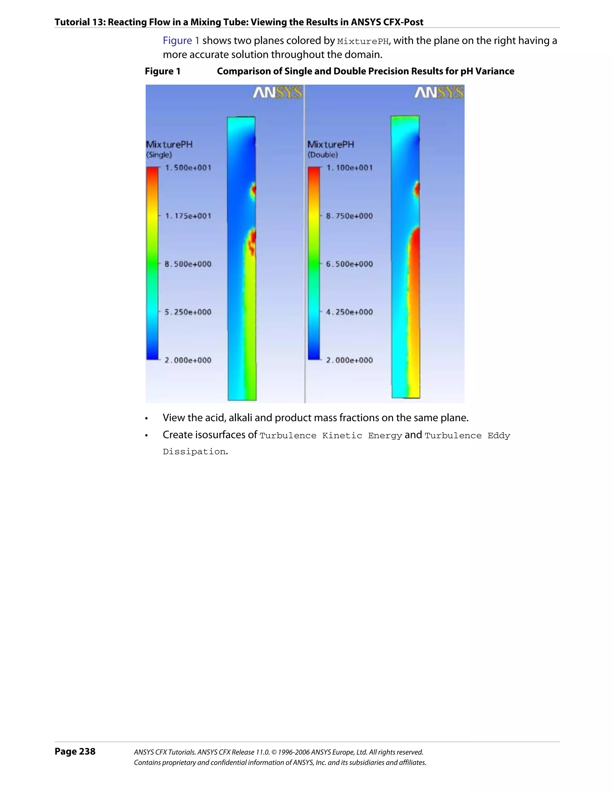

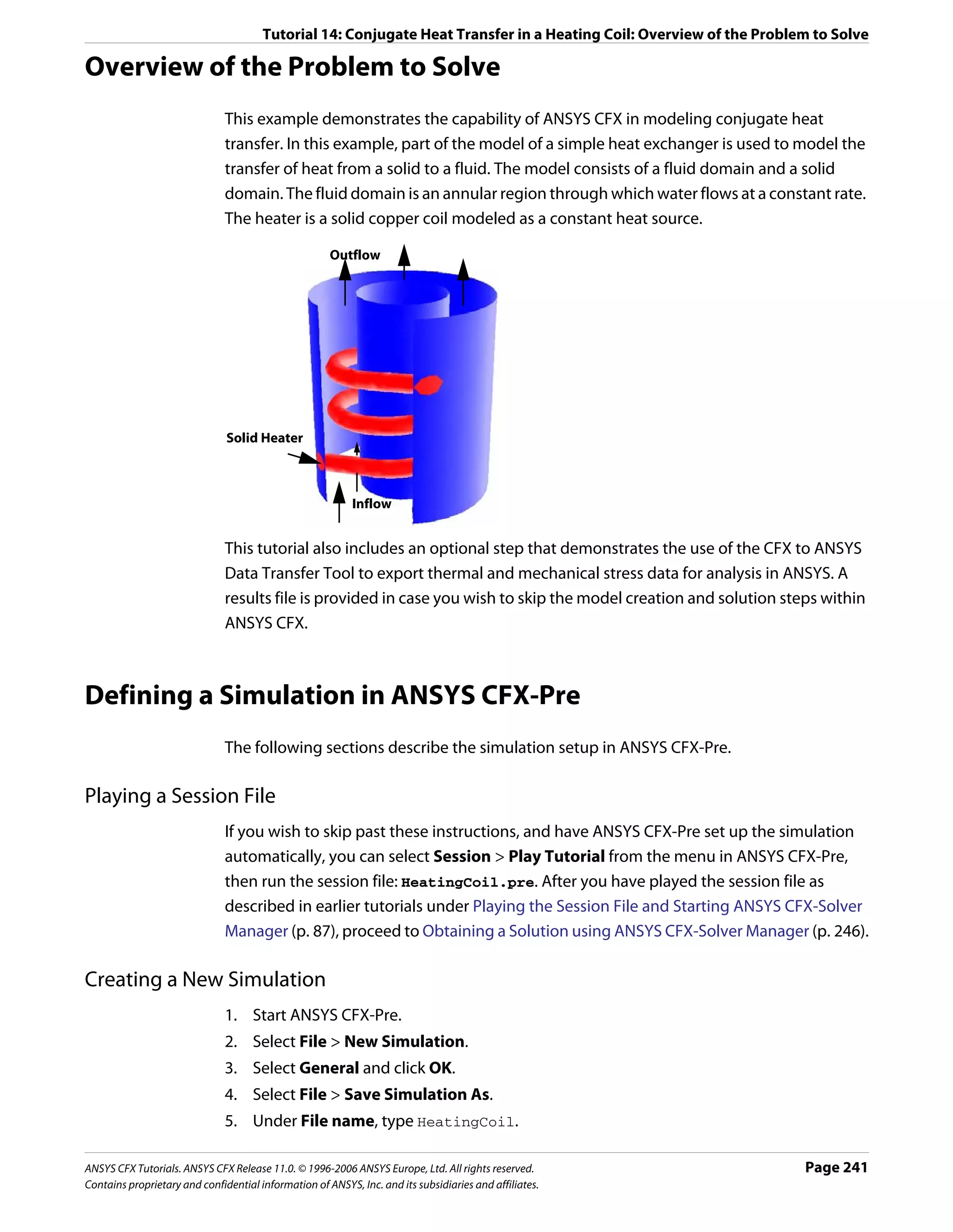
![Tutorial 14: Conjugate Heat Transfer in a Heating Coil: Defining a Simulation in ANSYS CFX-Pre
6. Click Save.
Importing the Mesh
1. Right-click Mesh and select Import Mesh.
2. Apply the following settings
Setting Value
File name HeatingCoilMesh.gtm
3. Click Open.
4. Right-click a blank area in the viewer and select Predefined Camera > Isometric View
(Z up) from the shortcut menu.
Creating the Domains
This simulation requires both a fluid and a solid domain. First, you will create a fluid domain
for the annular region of the heat exchanger.
Creating a Fluid The fluid domain will include the region of fluid flow but exclude the solid copper heater.
Domain
1. Click Domain and set the name to FluidZone.
2. Apply the following settings to FluidZone
Tab Setting Value
General Basic Settings > Location B1.P3*
Options
Basic Settings > Fluids List Water
Domain Models > Pressure > Reference Pressure 1 [atm]
Fluid Models Heat Transfer > Option Thermal Energy
Initialization Domain Initialization (Selected)
Domain Initialization > Initial Conditions (Selected)
Domain Initialization > Initial Conditions > Turbulence (Selected)
Eddy Dissipation
*. This region name may be different depending on how the mesh was created. You
should pick the region that forms the exterior surface of the volume surrounding
the coil.
3. Click OK.
Creating a Solid Since you know that the copper heating element will be much hotter than the fluid, you can
Domain initialize the temperature to a reasonable value. The initialization option that is set when
creating a domain applies only to that domain.
1. Create a new domain named SolidZone.
2. Apply the following settings
Page 242 ANSYS CFX Tutorials. ANSYS CFX Release 11.0. © 1996-2006 ANSYS Europe, Ltd. All rights reserved.
Contains proprietary and confidential information of ANSYS, Inc. and its subsidiaries and affiliates.](https://image.slidesharecdn.com/ansys11tutorial-111218135319-phpapp01/75/Ansys-11-tutorial-254-2048.jpg)
![Tutorial 14: Conjugate Heat Transfer in a Heating Coil: Defining a Simulation in ANSYS CFX-Pre
Tab Setting Value
General Basic Settings > Location B2.P3
Options
Basic Settings > Domain Type Solid Domain
Basic Settings > Solids List Copper
Solid Models Heat Transfer > Option Thermal Energy
Initialization Domain Initialization (Selected)
Domain Initialization > Initial Conditions (Selected)
Domain Initialization > Initial Conditions > Automatic with
Temperature > Option Value
Domain Initialization > Initial Conditions > 550 [K]
Temperature > Temperature
3. Click OK.
Creating a Subdomain to Specify a Thermal Energy Source
To allow a thermal energy source to be specified for the copper heating element, you need
to create a subdomain.
1. Create a new subdomain named Heater in the domain SolidZone.
2. Apply the following settings
Tab Setting Value
Basic Settings Basic Settings > Location B2.P3*
Sources Sources (Selected)
Sources > Equation Sources > Energy (Selected)
Sources > Equation Sources > Energy > Source 1.0E+07 [W m^-3]
*. This is the same location as for the domain SolidZone, because you want the source
term to apply to the entire solid domain.
3. Click OK.
Creating the Boundary Conditions
Inlet Boundary You will now create an inlet boundary condition for the cooling fluid (Water).
1. Create a new boundary condition named inflow in the domain FluidZone.
2. Apply the following settings
Tab Setting Value
Basic Settings Boundary Type Inlet
Location inflow
Boundary Details Mass and Momentum > Normal Speed 0.4 [m s^-1]
Heat Transfer > Static Temperature 300 [K]
3. Click OK.
ANSYS CFX Tutorials. ANSYS CFX Release 11.0. © 1996-2006 ANSYS Europe, Ltd. All rights reserved. Page 243
Contains proprietary and confidential information of ANSYS, Inc. and its subsidiaries and affiliates.](https://image.slidesharecdn.com/ansys11tutorial-111218135319-phpapp01/75/Ansys-11-tutorial-255-2048.jpg)
![Tutorial 14: Conjugate Heat Transfer in a Heating Coil: Defining a Simulation in ANSYS CFX-Pre
Opening The opening boundary condition type is used in this case because at some stage during the
boundary solution, the coiled heating element will cause some recirculation at the exit. At an opening
boundary you need to set the temperature of fluid that enters through the boundary. In this
case it is useful to base this temperature on the fluid temperature at the outlet, since you
expect the fluid to be flowing mostly out through this opening.
1. Create a new expression named OutletTemperature.
2. Set Definition to areaAve(T)@REGION:outflow
3. Click Apply.
4. Create a new boundary condition named outflow in the domain FluidZone.
5. Apply the following settings:
Tab Setting Value
Basic Settings Boundary Type Opening
Location outflow
Boundary Details Mass and Momentum > Option Opening Pres. and Dirn
Mass and Momentum > Relative Pressure 0 [Pa]
Heat Transfer > Option Static Temperature
Heat Transfer > Static Temperature OutletTemperature
6. Click OK.
The default adiabatic wall boundary condition will automatically be applied to the
remaining unspecified external boundaries of the fluid domain. The default Fluid-Solid
Interface boundary condition (flux conserved) will be applied to the surfaces between
the solid domain and the fluid domain.
Creating the Domain Interface
If you have the Generate Default Domain Interfaces option turned on (from Edit >
Options > CFX-Pre), then you will see that an interface called
Default Fluid Solid Interface already exists, and is listed in the Outline tree view. If
this is the case, you can optionally skip the following instructions for creating a domain
interface (since the domain interface set here will have the same settings as, and will
automatically replace, the default domain interface).
If you have the Generate Default Domain Interfaces option turned off, then there is no
domain interface defined at this point. In this case, create a domain interface using either
one of the following methods (the result is the same):
Creating a 1. Right click Simulation in the Outline tree view and ensure that Automatic Default
Default Domain Interfaces is selected. An interface named Default Fluid Solid Interface should
Interface
now appear under the Simulation branch.
Creating a 1. Double click Default Fluid Solid Interface and apply the following settings:
Domain
Interface
Manually
Page 244 ANSYS CFX Tutorials. ANSYS CFX Release 11.0. © 1996-2006 ANSYS Europe, Ltd. All rights reserved.
Contains proprietary and confidential information of ANSYS, Inc. and its subsidiaries and affiliates.](https://image.slidesharecdn.com/ansys11tutorial-111218135319-phpapp01/75/Ansys-11-tutorial-256-2048.jpg)
![Tutorial 14: Conjugate Heat Transfer in a Heating Coil: Defining a Simulation in ANSYS CFX-Pre
Tab Setting Value
Basic Settings Interface Type Fluid Solid
Interface Side 1 > Domain (Filter) FluidZone
Interface Side 1 > Region List F10.B1.P3, F5.B1.P3,
F6.B1.P3, F7.B1.P3, F8.B1.P3,
F9.B1.P3
Interface Side 2 > Domain (Filter) SolidZone
Interface Side 2 > Region List F10.B2.P3, F5.B2.P3,
F6.B2.P3, F7.B2.P3, F8.B2.P3,
F9.B2.P3
Interface Models > Option General Connection
Interface Models > Frame Change/Mixing None
Model > Option
Interface Models > Pitch Change > Option None
Mesh Connection Method > Option Automatic
2. Click OK.
Setting Solver Control
1. Click Solver Control .
2. Apply the following settings:
Tab Setting Value
Basic Settings Convergence Control > Fluid Timescale Physical Timescale
Control > Timescale Control
Convergence Control >Fluid Timescale 2 [s]
Control > Physical Timescale
For the Convergence Criteria, an RMS value of at least 1e-05 is usually required for
adequate convergence, but the default value is sufficient for demonstration purposes.
3. Click OK.
Writing the Solver (.def) File
1. Click Write Solver File .
2. Apply the following settings:
Setting Value
File name HeatingCoil.def
Quit CFX–Pre * (Selected)
*. If using ANSYS CFX-Pre in Standalone Mode.
3. Ensure Start Solver Manager is selected and click Save.
ANSYS CFX Tutorials. ANSYS CFX Release 11.0. © 1996-2006 ANSYS Europe, Ltd. All rights reserved. Page 245
Contains proprietary and confidential information of ANSYS, Inc. and its subsidiaries and affiliates.](https://image.slidesharecdn.com/ansys11tutorial-111218135319-phpapp01/75/Ansys-11-tutorial-257-2048.jpg)
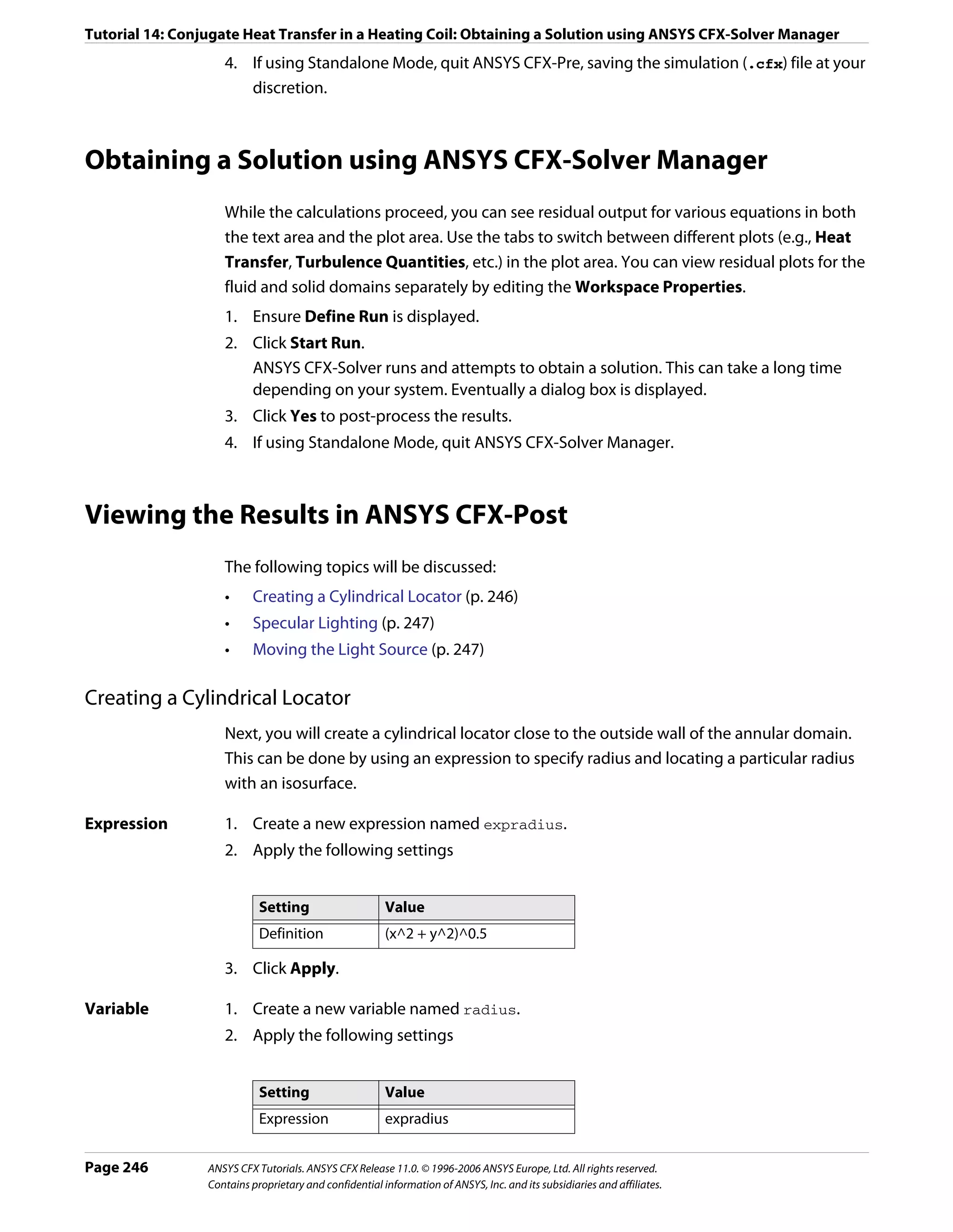
![Tutorial 14: Conjugate Heat Transfer in a Heating Coil: Exporting the Results to ANSYS
3. Click Apply.
Isosurface of the 1. Create a new isosurface named Isosurface 1.
variable 2. Apply the following settings
Tab Setting Value
Geometry Definition > Variable radius
Definition > Value 0.8 [m]*
Color Mode Variable
Variable Temperature
Range User Specified
Min 300 [K]
Max 302 [K]
Render Draw Faces (Selected)
*. The maximum radius is 1 m, so a cylinder locator at a radius of 0.8 m is suitable.
3. Click Apply.
Specular Lighting
Specular lighting is on by default. Specular lighting allows glaring bright spots on the
surface of an object, depending on the orientation of the surface and the position of the
light.
1. Apply the following settings to Isosurface 1
Tab Setting Value
Render Draw Faces > Specular (Cleared)
2. Click Apply.
Moving the Light Source
To move the light source, click within the 3-D Viewer, then press and hold <Shift> while
pressing the arrow keys left, right, up or down.
Tip: If using the Standalone version, you can move the light source by positioning the
mouse pointer in the viewer, holding down the <Ctrl> key, and dragging using the right
mouse button.
Exporting the Results to ANSYS
This optional step involves generating an ANSYS .cdb data file from the results generated
in ANSYS CFX-Solver. The .cdb file could then be used with the ANSYS Multi-field solver to
measure the combined effects of thermal and mechanical stresses on the solid heating coil.
There are two possible ways to export data to ANSYS:
ANSYS CFX Tutorials. ANSYS CFX Release 11.0. © 1996-2006 ANSYS Europe, Ltd. All rights reserved. Page 247
Contains proprietary and confidential information of ANSYS, Inc. and its subsidiaries and affiliates.](https://image.slidesharecdn.com/ansys11tutorial-111218135319-phpapp01/75/Ansys-11-tutorial-259-2048.jpg)
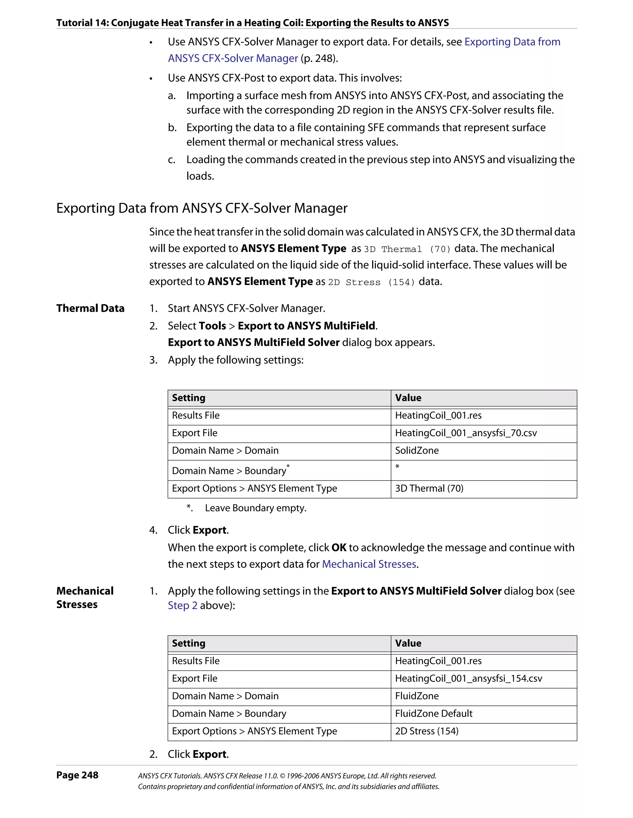


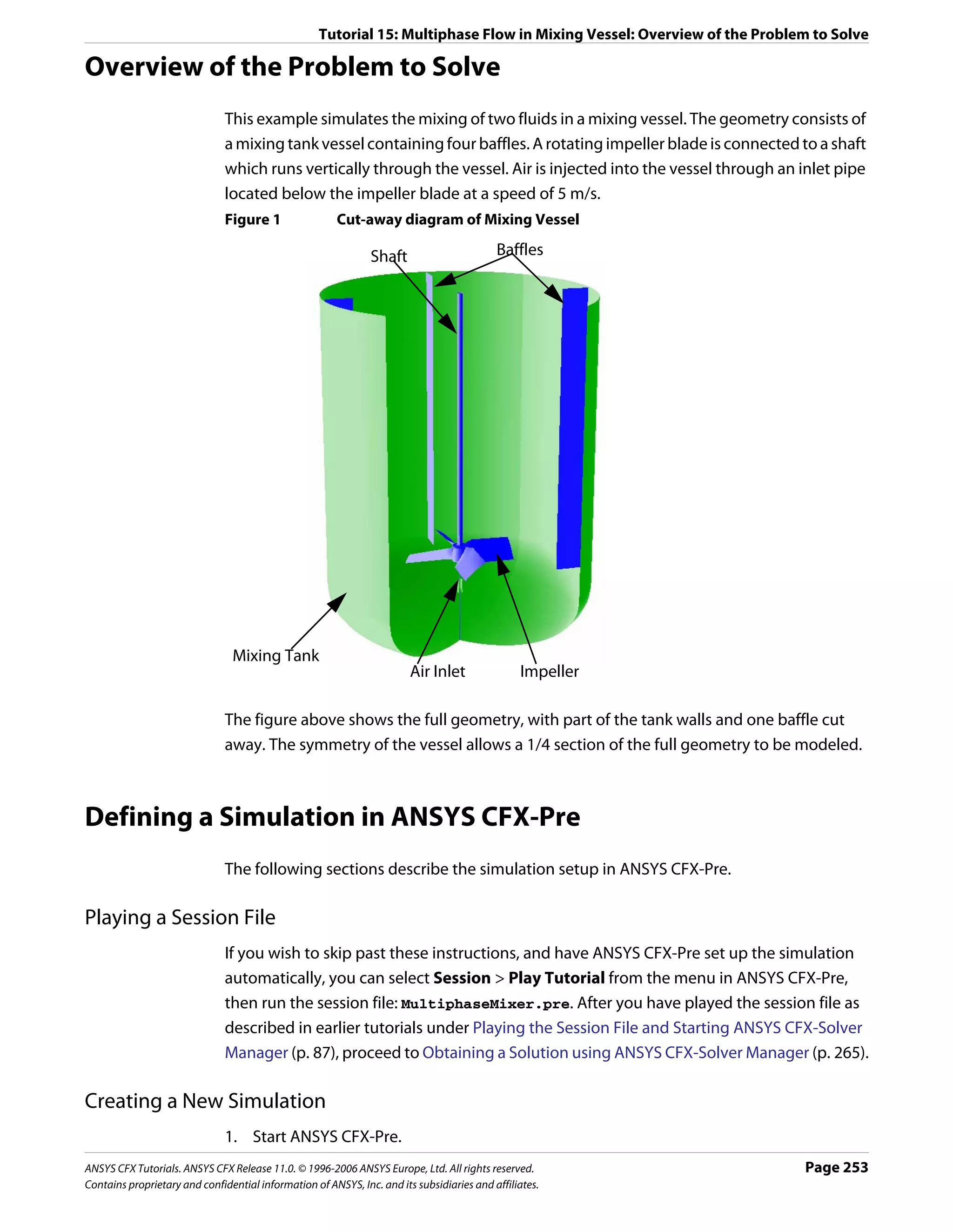
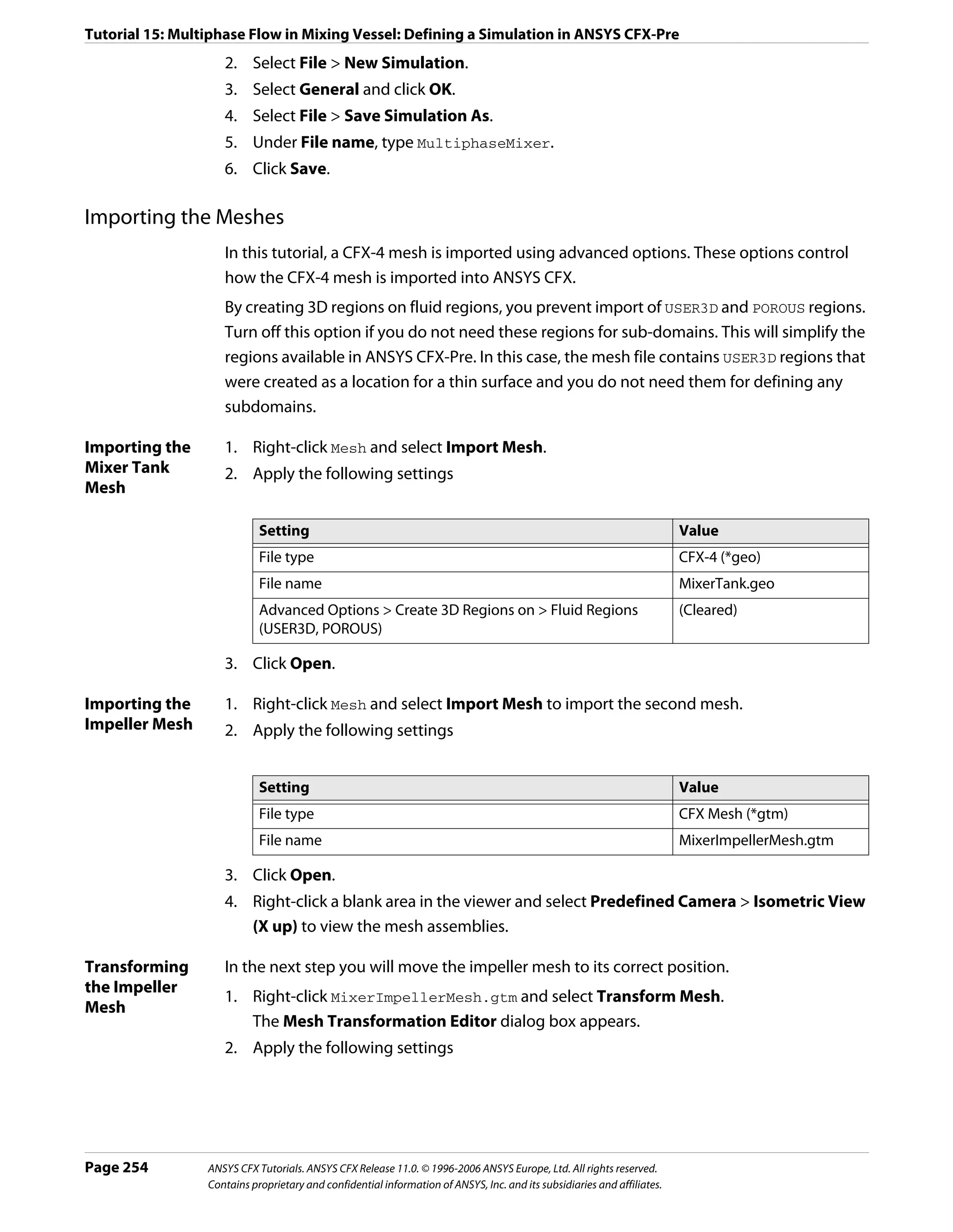
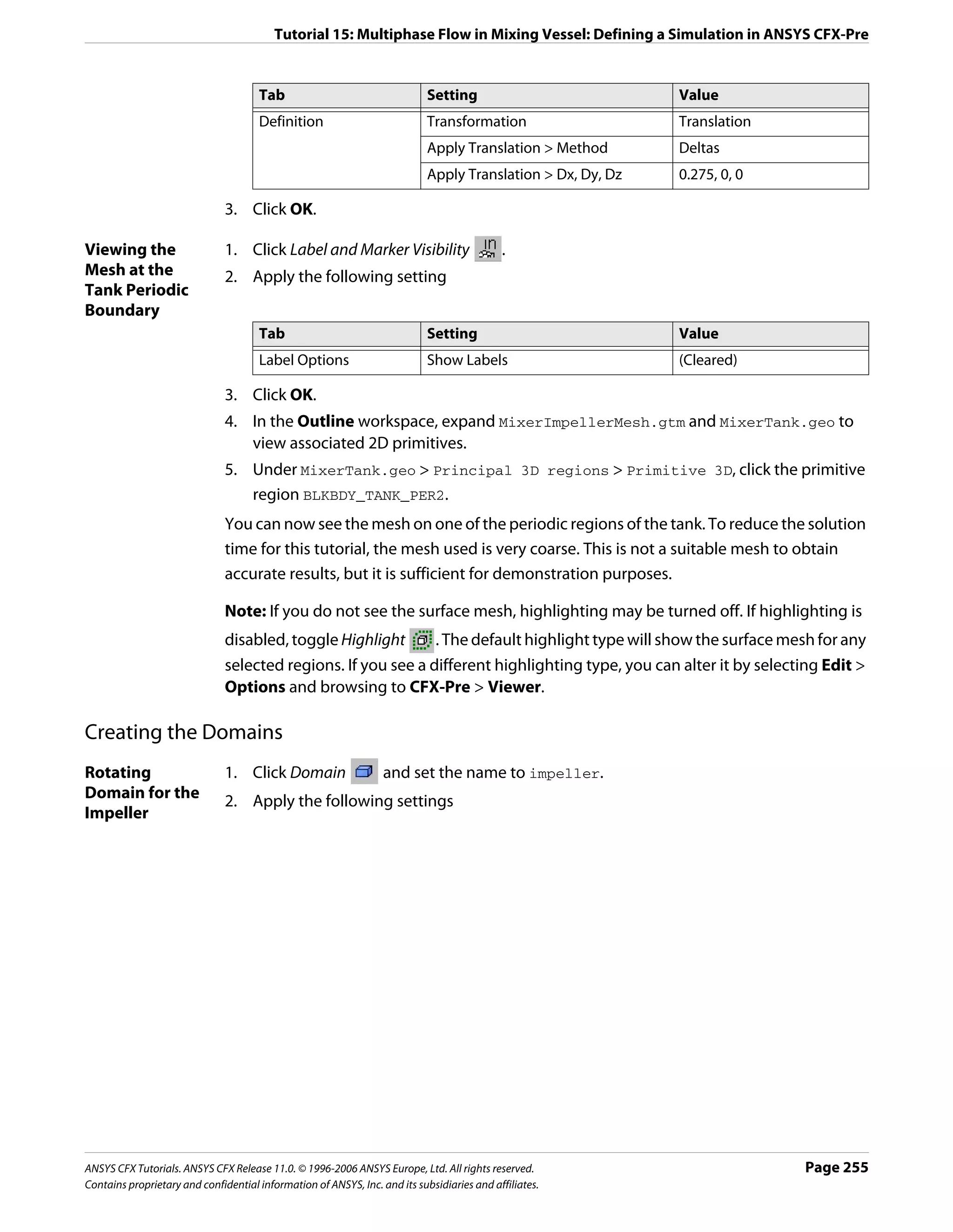
![Tutorial 15: Multiphase Flow in Mixing Vessel: Defining a Simulation in ANSYS CFX-Pre
Tab Setting Value
General Basic Settings > Location Main
Options
Basic Settings > Fluids List Air at 25 C, Water
Domain Models > Pressure > Reference Pressure 1 [atm]
Domain Models > Buoyancy > Option Buoyant
Domain Models > Buoyancy > Gravity X Dirn. -9.81 [m s^-2]
Domain Models > Buoyancy > Gravity Y Dirn. 0 [m s^-2]
Domain Models > Buoyancy > Gravity Z Dirn. 0 [m s^-2]
Domain Models > Buoyancy > Buoy. Ref. Density* 997 [kg m^-3]
Domain Models > Domain Motion > Option Rotating
Domain Models > Domain Motion > Angular Velocity 84 [rev min-1]†
Domain Models > Domain Motion > Axis Definition > Global X
Rotation Axis
Fluid Multiphase Options > Homogeneous Model (Cleared)
Models Multiphase Options > Allow Musig Fluids (Cleared)
Multiphase Options > Free Surface Model > Option None
Heat Transfer > Homogeneous Model (Cleared)
Heat Transfer > Option Isothermal
Heat Transfer > Fluid Temperature 25 [C]
Turbulence > Homogeneous Model (Cleared)
Turbulence > Option Fluid Dependent
Fluid Fluid Details Air at 25 C
Details
Fluid Details > Air at 25 C > Morphology > Option Dispersed Fluid
Fluid Details > Air at 25 C > Morphology > Mean Diameter 3 [mm]
Fluid Fluid Pairs Air at 25 C | Water
Pairs Fluid Pairs > Air at 25 C | Water > Surface Tension Coefficient (Selected)
Fluid Pairs > Air at 25 C | Water > Surface Tension Coefficient 0.073 [N m^-1]‡
> Surf. Tension Coeff.
Fluid Pairs > Air at 25 C | Water > Momentum Transfer > Drag Grace
Force > Option
Fluid Pairs > Air at 25 C | Water > Momentum Transfer > Drag (Selected)
Force > Volume Fraction Correction Exponent
Fluid Pairs > Air at 25 C | Water > Momentum Transfer > Drag 4
Force > Volume Fraction Correction Exponent > Value
Fluid Pairs > Air at 25 C | Water > Momentum Transfer > Lopez de
Non-drag forces > Turbulent Dispersion Force > Option Bertodano
Fluid Pairs > Air at 25 C | Water > Momentum Transfer > 0.1
Non-drag forces > Turbulent Dispersion Force > Dispersion
Coeff.
Fluid Pairs > Air at 25 C | Water > Turbulence Transfer > Sato Enhanced
Option Eddy Viscosity
Page 256 ANSYS CFX Tutorials. ANSYS CFX Release 11.0. © 1996-2006 ANSYS Europe, Ltd. All rights reserved.
Contains proprietary and confidential information of ANSYS, Inc. and its subsidiaries and affiliates.](https://image.slidesharecdn.com/ansys11tutorial-111218135319-phpapp01/75/Ansys-11-tutorial-268-2048.jpg)

![Tutorial 15: Multiphase Flow in Mixing Vessel: Defining a Simulation in ANSYS CFX-Pre
Tab Setting Value
Fluid Values Boundary Conditions Air at 25 C
Boundary Conditions > Air at 25 C > Velocity 5 [m s^-1]
> Normal Speed
Boundary Conditions > Air at 25 C > Volume 1
Fraction > Volume Fraction
Boundary Conditions Water
Boundary Conditions > Water > Velocity > 5 [m s^-1]
Normal Speed
Boundary Conditions > Water > Volume 0
Fraction > Volume Fraction
3. Click OK.
Degassing 1. Create a new boundary condition in the domain tank named LiquidSurface.
Outlet 2. Apply the following settings
Boundary
Tab Setting Value
Basic Settings Boundary Type Outlet
Location WALL_LIQUID_SURFACE
Boundary Details Mass and Momentum > Option Degassing Condition
3. Click OK.
Thin Surface for In ANSYS CFX-Pre, thin surfaces can be created by specifying wall boundary conditions on
the Baffle both sides of internal 2D regions. Both sides of the baffle regions will be specified as walls in
this case.
1. Create a new boundary condition in the domain tank named Baffle.
2. Apply the following settings
Tab Setting Value
Basic Settings Boundary Type Wall
Location WALL_BAFFLES*
Boundary Details Wall Influence On Flow > Option Fluid Dependent
Fluid Values Boundary Conditions Air at 25 C
Boundary Conditions > Air at 25 C > Wall Free Slip
Influence on Flow > Option
Boundary Conditions Water
Boundary Conditions > Water > Wall No Slip†
Influence on Flow > Option
*. The WALL_BAFFLES region includes the surfaces on both sides of the baffle (you can
confirm this by examining WALL_BAFFLES in the region selector). Therefore, you do
not need to use the Create Thin Surface Partner option.
†. The Free Slip condition can be used for the gas phase since the contact area with
the walls is near zero for low gas phase volume fractions.
3. Click OK.
Page 258 ANSYS CFX Tutorials. ANSYS CFX Release 11.0. © 1996-2006 ANSYS Europe, Ltd. All rights reserved.
Contains proprietary and confidential information of ANSYS, Inc. and its subsidiaries and affiliates.](https://image.slidesharecdn.com/ansys11tutorial-111218135319-phpapp01/75/Ansys-11-tutorial-270-2048.jpg)
![Tutorial 15: Multiphase Flow in Mixing Vessel: Defining a Simulation in ANSYS CFX-Pre
Wall Boundary The next stage involves setting up a boundary condition for the shaft, which exists in the
Condition for tank (stationary domain). These regions are connected to the shaft in the impeller domain.
the Shaft
Since the tank domain is not rotating, you need to specify a moving wall to account for the
rotation of the shaft.
Part of the shaft is located directly above the air inlet, so the volume fraction of air in this
location will be high and the assumption of zero contact area for the gas phase is not
physically correct. In this case, a no slip boundary condition is more appropriate than a free
slip condition for the air phase. When the volume fraction of air in contact with a wall is low,
a free slip condition is more appropriate for the air phase.
In cases where it is important to correctly model the dispersed phase slip properties at walls
for all volume fractions, you can declare both fluids as no slip, but set up an expression for
the dispersed phase wall area fraction. The expression should result in an area fraction of
zero for dispersed phase volume fractions from 0 to 0.3, for example, and then linearly
increase to an area fraction of 1 as the volume fraction increases to 1.
1. Create a new boundary condition in the domain tank named TankShaft.
2. Apply the following settings
Tab Setting Value
Basic Settings Boundary Type Wall
Location WALL_SHAFT,
WALL_SHAFT_CENTER
Boundary Details Wall Influence On Flow > Option Fluid Dependent
Fluid Values Boundary Conditions Air at 25 C
Boundary Conditions > Air at 25 C > Wall No Slip
Influence on Flow > Option
Boundary Conditions > Air at 25 C > Wall (Selected)
Influence on Flow > Wall Velocity
Boundary Conditions > Air at 25 C > Wall Rotating Wall
Influence on Flow > Wall Velocity > Option
Boundary Conditions > Air at 25 C > Wall 84 [rev min-1]*
Influence on Flow > Wall Velocity > Angular
Velocity
Boundary Conditions > Air at 25 C > Wall Global X
Influence on Flow > Wall Velocity > Axis
Definition > Rotation Axis
*. Note the unit.
3. Select Water and set the same values as for Air at 25 C.
4. Click OK.
Required 1. Create a new boundary condition in the domain impeller named Blade.
Boundary 2. Apply the following settings
Conditions in
the Impeller
Domain
ANSYS CFX Tutorials. ANSYS CFX Release 11.0. © 1996-2006 ANSYS Europe, Ltd. All rights reserved. Page 259
Contains proprietary and confidential information of ANSYS, Inc. and its subsidiaries and affiliates.](https://image.slidesharecdn.com/ansys11tutorial-111218135319-phpapp01/75/Ansys-11-tutorial-271-2048.jpg)
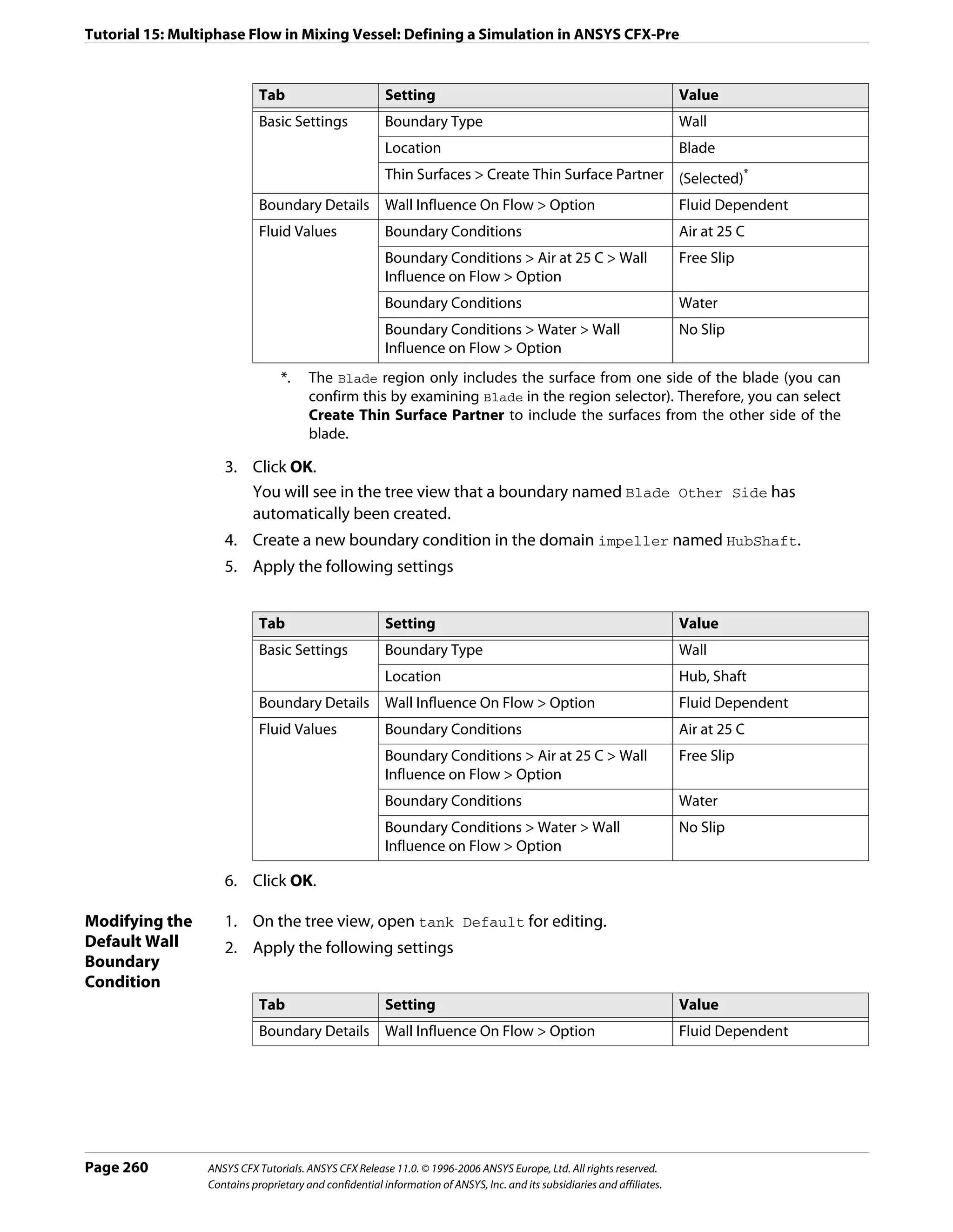
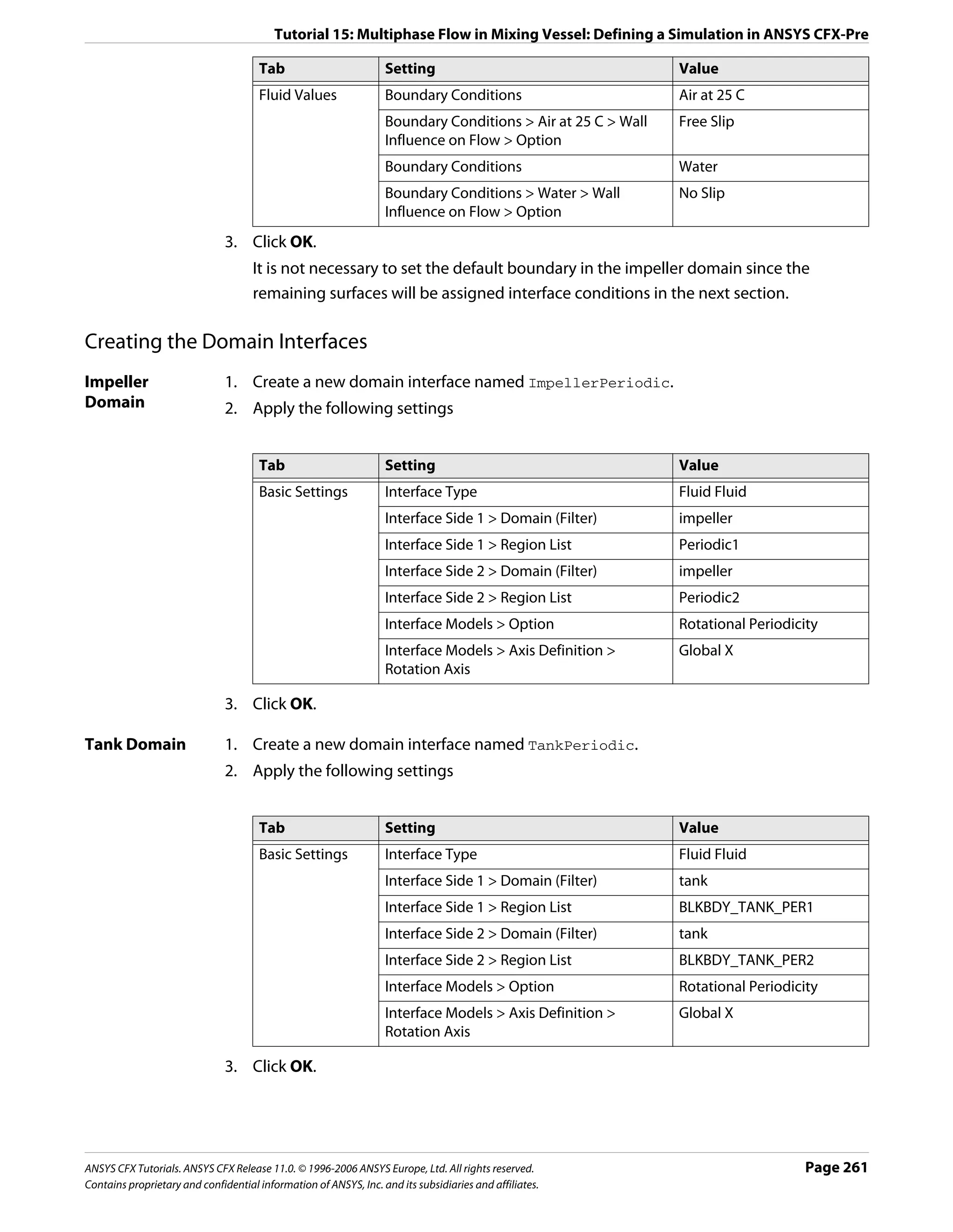
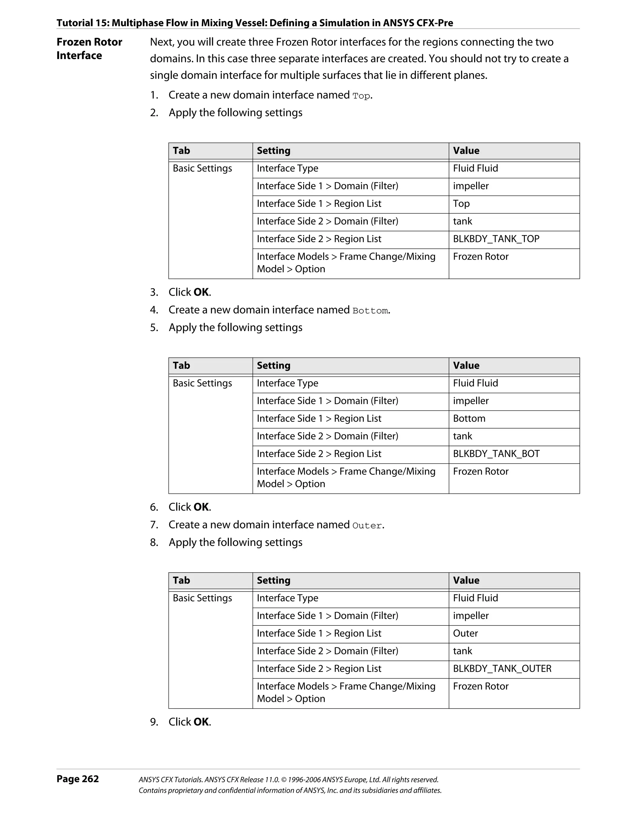
![Tutorial 15: Multiphase Flow in Mixing Vessel: Defining a Simulation in ANSYS CFX-Pre
Setting Initial Values
The initialization for volume fraction is 0 for air and automatic for water. Therefore, the initial
volume fraction for water will be set to 1 so that the sum of the two fluid volume fractions is
1.
It is important to understand how the velocity is initialized in this tutorial. Here, both fluids
use Automatic for the Cartesian Velocity Components. When the Automatic option is
used, the initial velocity field will be based on the velocity values set at inlets, openings, and
outlets. In this tutorial, the only boundary that has a set velocity value is the inlet, which
specifies a velocity of 5 [m s^-1] for both phases. Without setting the Velocity Scale
parameter, the resulting initial guess would be a uniform velocity of 5 [m s^-1] in the
X-direction throughout the domains for both phases. This is clearly not suitable since the
water phase is enclosed by the tank. When the boundary velocity conditions are not
representative of the expected domain velocities, the Velocity Scale parameter should be
used to set a representative domain velocity. In this case the velocity scale for water is set to
zero, causing the initial velocity for the water to be zero. The velocity scale is not set for air,
resulting in an initial velocity of 5 [m s^-1] in the X-direction for the air. This should not be a
problem since the initial volume fraction of the air is zero everywhere.
1. Click Global Initialization .
2. Apply the following settings
Tab Setting Value
Fluid Settings Fluid Specific Initialization Air at 25 C
Fluid Specific Initialization > Air at 25 C > Initial Automatic with Value
Conditions > Volume Fraction > Option
Fluid Specific Initialization > Air at 25 C > Initial 0
Conditions > Volume Fraction > Volume Fraction
Fluid Specific Initialization Water
Fluid Specific Initialization > Water > Initial (Selected)
Conditions > Cartesian Velocity Components >
Velocity Scale
Fluid Specific Initialization > Water > Initial 0 [m s^-1]
Conditions > Cartesian Velocity Components >
Velocity Scale > Value
Fluid Specific Initialization > Water > Initial (Selected)
Conditions > Turbulence Eddy Dissipation
3. Click OK.
Setting Solver Control
Generally, two different time scales exist for multiphase mixers. The first is a small time scale
based on the rotational speed of the impeller, typically taken as 1 / ω , resulting in a time
scale of 0.11 s for this case. The second time scale is usually larger and based on the
recirculation time of the continuous phase in the mixer.
ANSYS CFX Tutorials. ANSYS CFX Release 11.0. © 1996-2006 ANSYS Europe, Ltd. All rights reserved. Page 263
Contains proprietary and confidential information of ANSYS, Inc. and its subsidiaries and affiliates.](https://image.slidesharecdn.com/ansys11tutorial-111218135319-phpapp01/75/Ansys-11-tutorial-275-2048.jpg)
![Tutorial 15: Multiphase Flow in Mixing Vessel: Defining a Simulation in ANSYS CFX-Pre
Using a timestep based on the rotational speed of the impeller will be more robust, but
convergence will be slow since it takes time for the flow field in the mixer to develop. Using
a larger timestep reduces the number of iterations required for the mixer flow field to
develop, but reduces robustness. You will need to experiment to find an optimum timestep.
Note: You may find it useful to monitor the value of an expression during the solver run so
that you can view the volume fraction of air in the tank (the gas hold up). The gas hold up is
often used to judge convergence in these types of simulations by converging until a
steady-state value is achieved. You could create the following expressions:
TankAirHoldUp = volumeAve(Air at 25 C.vf)@tank
ImpellerAirHoldUp = volumeAve(Air at 25 C.vf)@impeller
TotalAirHoldUp = (volume()@tank * TankAirHoldUp + volume()@impeller *
ImpellerAirHoldUp) / (volume()@tank + volume()@impeller)
and then monitor the value of TotalAirHoldUp.
1. Click Solver Control .
2. Apply the following settings
Tab Setting Value
Basic Settings Convergence Control > Fluid Timescale Physical Timescale
Control > Timescale Control
Convergence Control > Fluid Timescale 2 [s]*
Control > Physical Timescale
*. This is an aggressive timestep for this case.
3. Click OK.
Setting Output Control
In the next step, you will choose to write additional data to the results file which allows force
and torque calculations to be performed in post-processing.
1. Click Output Control .
2. Apply the following settings
Tab Setting Value
Results Output Boundary Flows (Selected)
Output Boundary Flows > Boundary Flows All
3. Click OK.
Writing the Solver (.def) File
Since this tutorial uses domain interfaces and you choose to summarize the interface data,
an information window is displayed that informs you of the connection type used for each
domain interface.
1. Click Write Solver File .
2. Apply the following settings:
Page 264 ANSYS CFX Tutorials. ANSYS CFX Release 11.0. © 1996-2006 ANSYS Europe, Ltd. All rights reserved.
Contains proprietary and confidential information of ANSYS, Inc. and its subsidiaries and affiliates.](https://image.slidesharecdn.com/ansys11tutorial-111218135319-phpapp01/75/Ansys-11-tutorial-276-2048.jpg)

![Tutorial 15: Multiphase Flow in Mixing Vessel: Viewing the Results in ANSYS CFX-Post
Visualizing the Mixing Process
Creating a plane 1. Create a new plane named Plane 1.
2. Apply the following settings
Tab Setting Value
Geometry Definition > Method Three Points
Definition > Point 1 1, 0, 0
Definition > Point 2 0, 1, -0.9
Definition > Point 3 0, 0, 0
Color Mode Variable
Variable Air at 25 C.Volume Fraction
Range User Specified
Min 0
Max 0.04
3. Click Apply.
4. Observe the plane, then apply the following settings:
Tab Setting Value
Color Variable Air at 25 C.Shear Strain Rate
Range User Specified
Min 0 [s^-1]
Max 15 [s^-1]
5. Click Apply.
Areas of high shear strain rate or shear stress are typically also areas where the highest
mixing occurs.
6. Observe the plane, then apply the following settings:
Tab Setting Value
Color Variable Pressure
Range Local
7. Click Apply.
Note that the hydrostatic contribution to pressure is excluded due to the use of an
appropriate buoyancy reference density. If you plot the variable called Absolute
Pressure, you will see the true pressure including the hydrostatic contribution.
Creating a 1. Create a new vector named Vector 1.
vector 2. Apply the following settings
Page 266 ANSYS CFX Tutorials. ANSYS CFX Release 11.0. © 1996-2006 ANSYS Europe, Ltd. All rights reserved.
Contains proprietary and confidential information of ANSYS, Inc. and its subsidiaries and affiliates.](https://image.slidesharecdn.com/ansys11tutorial-111218135319-phpapp01/75/Ansys-11-tutorial-278-2048.jpg)
![Tutorial 15: Multiphase Flow in Mixing Vessel: Viewing the Results in ANSYS CFX-Post
Tab Setting Value
Geometry Definition > Locations Plane 1
Variable Water.Velocity in Stn Frame*
Symbol Symbol Size 0.2
Normalize Symbols (Selected)
*. Using this variable, instead of Water.Velocity, results in the velocity vectors
appearing to be continuous at the interface between the rotating and stationary
domains. Velocity variables that do not include a frame specification always use the
local reference frame.
3. Observe the vector plot, then change the variable to Air at 25 C.Velocity in Stn
Frame. Observe this as well, then clear the visibility of Vector 1.
4. Modify the tank Default object.
5. Apply the following settings:
Tab Setting Value
Color Mode Variable
Variable Water.Wall Shear
Range Local
The legend for this plot shows the range of wall shear values.
The global maximum wall shear is much higher than the maximum value on the default
walls. The global maximum values occur on the TankShaft boundary directly above the
inlet. Although these values are very high, the shear force exerted on this boundary will
be small since the contact area fraction of water here is very small.
Calculating 1. Select Tools > Function Calculator from the main menu or click Show Function
Power and
Calculator from the main toolbar.
Torque
Required by the 2. Apply the following settings:
Impeller
Tab Setting Value
Function Function torque
Calculator Location Blade
Axis Global X
Fluid All Fluids
3. Click Calculate to find the torque required to rotate Blade about the X-axis.
4. Repeat the calculation setting Location to Blade Other Side.
The sum of these two results is the torque required by the single impeller blade,
approximately 70 [N m]. This must be multiplied by the number of blades in the full
geometry to obtain the total torque required by the impeller; the result is a value of
approximately 282 [N m]. You could also include the results from the locations HubShaft
and TankShaft; however in this case their contributions are negligible.
ANSYS CFX Tutorials. ANSYS CFX Release 11.0. © 1996-2006 ANSYS Europe, Ltd. All rights reserved. Page 267
Contains proprietary and confidential information of ANSYS, Inc. and its subsidiaries and affiliates.](https://image.slidesharecdn.com/ansys11tutorial-111218135319-phpapp01/75/Ansys-11-tutorial-279-2048.jpg)
![Tutorial 15: Multiphase Flow in Mixing Vessel: Viewing the Results in ANSYS CFX-Post
The power requirement is simply the required torque multiplied by the rotational speed
(8.8 rad/s): Power = 282*8.8 = 2482 [W].
Remember that this value is the power requirement for the work done on the fluid only, it
does not account for any mechanical losses, efficiencies etc. Also note that the accuracy of
these results is significantly affected by the coarseness of the mesh. You should not use a
mesh of this length scale to obtain accurate quantitative results.
Page 268 ANSYS CFX Tutorials. ANSYS CFX Release 11.0. © 1996-2006 ANSYS Europe, Ltd. All rights reserved.
Contains proprietary and confidential information of ANSYS, Inc. and its subsidiaries and affiliates.](https://image.slidesharecdn.com/ansys11tutorial-111218135319-phpapp01/75/Ansys-11-tutorial-280-2048.jpg)

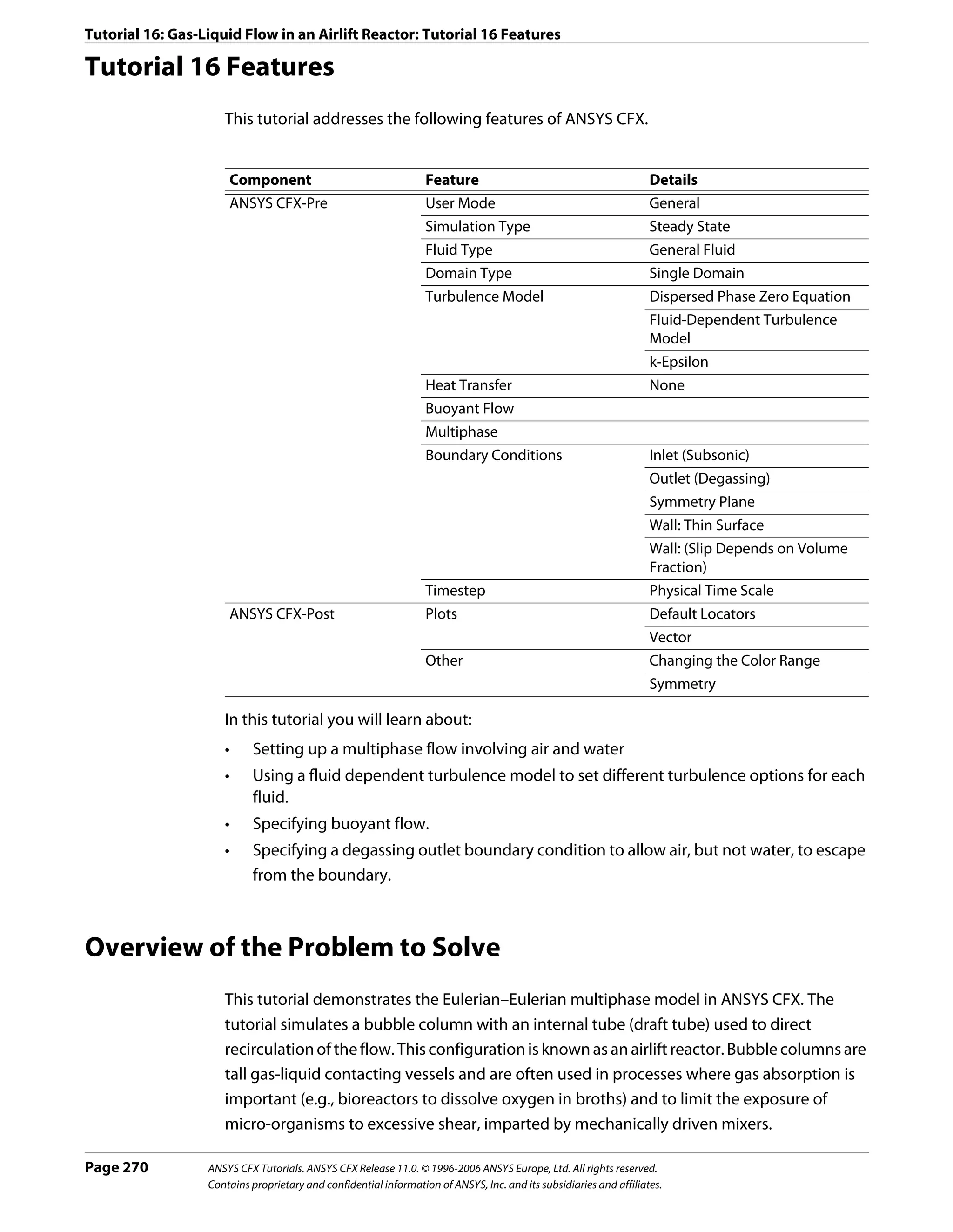
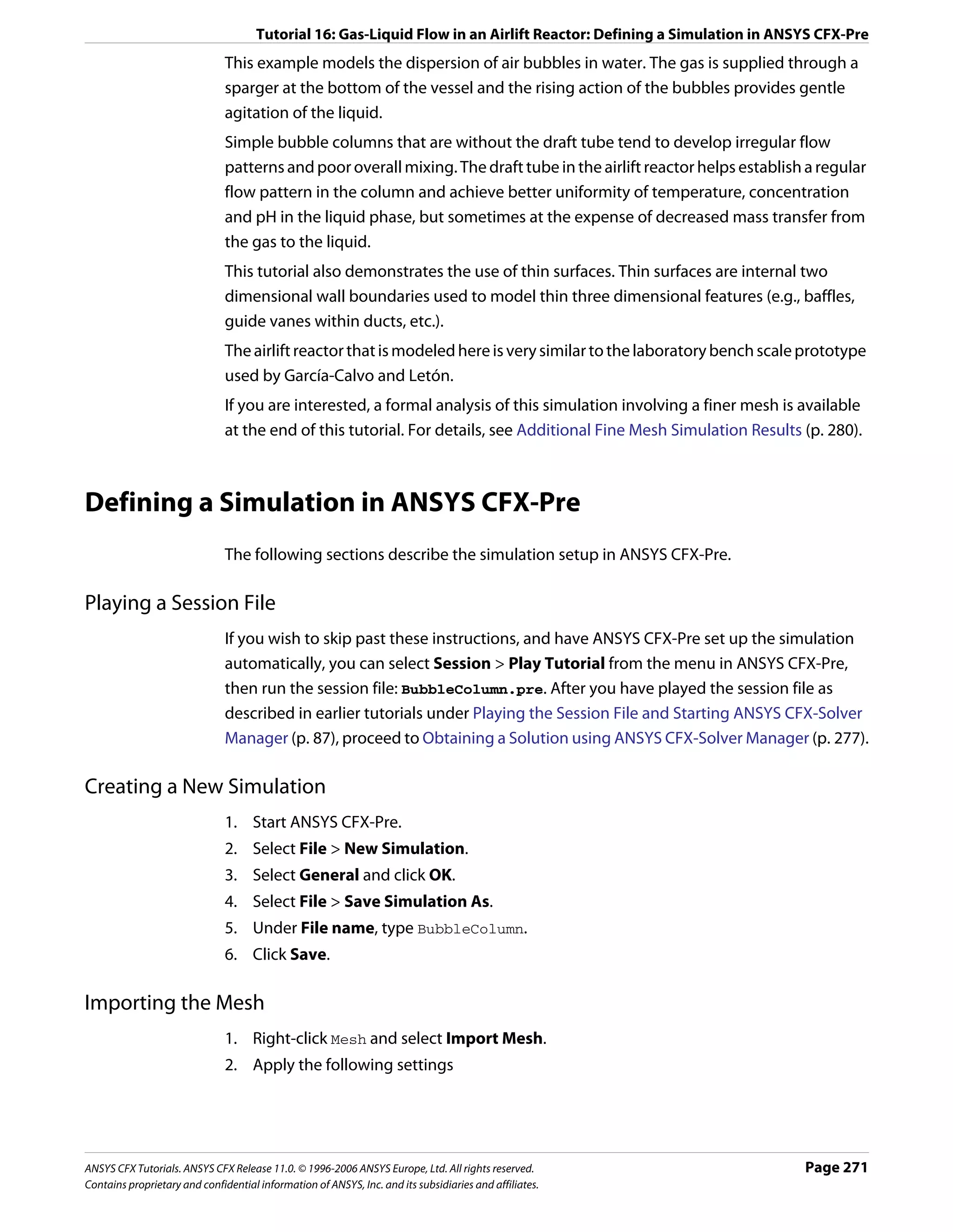
![Tutorial 16: Gas-Liquid Flow in an Airlift Reactor: Defining a Simulation in ANSYS CFX-Pre
Setting Value
File name BubbleColumnMesh.gtm
3. Click Open.
Creating the Domain
1. Right click Simulation in the Outline tree view and ensure that Automatic Default
Domain is selected. A domain named Default Domain should now appear under the
Simulation branch.
2. Double click Default Domain and apply the following settings:
Tab Setting Value
General Basic Settings > Location B1.P3, B2.P3
Options
Basic Settings > Fluids List Air at 25 C, Water
Domain Models > Pressure > Reference Pressure 1 [atm]
Domain Models > Buoyancy > Option Buoyant
Domain Models > Buoyancy > Gravity X Dirn. 0 [m s^-2]
Domain Models > Buoyancy > Gravity Y Dirn. -9.81 [m s^-2]
Domain Models > Buoyancy > Gravity Z Dirn. 0 [m s^-2]
Domain Models > Buoyancy > Buoy. Ref. Density* 997 [kg m^-3]
Fluid Multiphase Options > Homogeneous Model (Cleared)
Models
Multiphase Options > Allow Musig Fluids (Cleared)
Free Surface Model > Option None
Heat Transfer > Option Isothermal
Heat Transfer > Fluid Temperature 25 C
Turbulence > Option Fluid Dependent
Fluid Fluid Details Air at 25 C
Details Fluid Details > Air at 25 C > Morphology > Option Dispersed Fluid
Fluid Details > Air at 25 C > Morphology > Mean Diameter 6 [mm]
Page 272 ANSYS CFX Tutorials. ANSYS CFX Release 11.0. © 1996-2006 ANSYS Europe, Ltd. All rights reserved.
Contains proprietary and confidential information of ANSYS, Inc. and its subsidiaries and affiliates.](https://image.slidesharecdn.com/ansys11tutorial-111218135319-phpapp01/75/Ansys-11-tutorial-284-2048.jpg)
![Tutorial 16: Gas-Liquid Flow in an Airlift Reactor: Defining a Simulation in ANSYS CFX-Pre
Tab Setting Value
Fluid Fluid Pairs > Air at 25 C | Water > Surface Tension Coefficient (Selected)
Pairs Fluid Pairs > Air at 25 C | Water > Surface Tension Coefficient 0.072 [N m^-1]†
> Surf. Tension Coeff.
Fluid Pairs > Air at 25 C | Water > Momentum Transfer > Drag Grace
Force > Option
Fluid Pairs > Air at 25 C | Water > Momentum Transfer > Drag (Selected)
Force > Volume Fraction Correction Exponent
Fluid Pairs > Air at 25 C | Water > Momentum Transfer > Drag 2
Force > Volume Fraction Correction Exponent > Value
Fluid Pairs > Air at 25 C | Water > Momentum Transfer > Lopez de
Non-drag Forces > Turbulent Dispersion Force > Option Bertodano
Fluid Pairs > Air at 25 C | Water > Momentum Transfer > 0.3
Non-drag Forces > Turbulent Dispersion Force > Dispersion
Coeff.
Fluid Pairs > Air at 25 C | Water > Turbulence Transfer > Sato Enhanced
Option Eddy Viscosity
*. For dilute dispersed multiphase flow, always set the buoyancy reference density to
that for continuous fluid.
†. This must be set to allow the Grace drag model to be used.
3. Click OK.
Creating the Boundary Conditions
For this simulation of the airlift reactor, the boundary conditions required are:
• An inlet for air on the sparger.
• A degassing outlet for air at the liquid surface.
• A thin surface wall for the draft tube.
• An exterior wall for the outer wall, base and sparger tube.
• Symmetry planes for the cross sections.
Inlet Boundary There are an infinite number of inlet velocity/volume fraction combinations that will
produce the same mass inflow of air. The combination chosen gives an air inlet velocity
close to the terminal rise velocity. Since the water inlet velocity is zero, you can adjust its
volume fraction until the required mass flow rate of air is obtained for a given air inlet
velocity.
1. Create a new boundary condition named Sparger.
2. Apply the following settings
Tab Setting Value
Basic Settings Boundary Type Inlet
Location Sparger
Boundary Details Mass And Momentum > Option Fluid Dependent
ANSYS CFX Tutorials. ANSYS CFX Release 11.0. © 1996-2006 ANSYS Europe, Ltd. All rights reserved. Page 273
Contains proprietary and confidential information of ANSYS, Inc. and its subsidiaries and affiliates.](https://image.slidesharecdn.com/ansys11tutorial-111218135319-phpapp01/75/Ansys-11-tutorial-285-2048.jpg)
![Tutorial 16: Gas-Liquid Flow in an Airlift Reactor: Defining a Simulation in ANSYS CFX-Pre
Tab Setting Value
Fluid Values Boundary Conditions Air at 25 C
Boundary Conditions > Air at 25 C > Velocity 0.3 [m s^-1]
> Normal Speed
Boundary Conditions > Air at 25 C > Volume 0.25
Fraction > Volume Fraction
Boundary Conditions Water
Boundary Conditions > Water > Velocity > 0 [m s^-1]
Normal Speed
Boundary Conditions > Water > Volume 0.75
Fraction > Volume Fraction
3. Click OK.
Outlet The top of the reactor will be a degassing boundary, which is classified as an outlet
Boundary boundary.
1. Create a new boundary condition named Top.
2. Apply the following settings
Tab Setting Value
Basic Settings Boundary Type Outlet
Location Top
Boundary Details Mass and Momentum > Option Degassing Condition
3. Click OK.
Thin Surface Thin surfaces are created by specifying a wall boundary condition on both sides of an
Draft Tube internal region. If only one side has a boundary condition then the ANSYS CFX-Solver will
Boundary
fail. To assist with this, you can select only one side of a thin surface and then enable the
Create Thin Surface Partner toggle. ANSYS CFX-Pre will then try to automatically create
another boundary condition for the other side.
1. Create a new boundary condition named DraftTube.
2. Apply the following settings
Tab Setting Value
Basic Settings Boundary Type Wall
Location Draft Tube
Thin Surfaces > Create Thin Surface Partner (Selected)
Boundary Details Wall Influence On Flow > Option Fluid Dependent
Fluid Values Boundary Conditions Air at 25 C
Boundary Conditions > Air at 25 C > Wall Free Slip
Influence On Flow > Option
Boundary Conditions Water
Boundary Conditions > Water > Wall No Slip
Influence On Flow > Option
Page 274 ANSYS CFX Tutorials. ANSYS CFX Release 11.0. © 1996-2006 ANSYS Europe, Ltd. All rights reserved.
Contains proprietary and confidential information of ANSYS, Inc. and its subsidiaries and affiliates.](https://image.slidesharecdn.com/ansys11tutorial-111218135319-phpapp01/75/Ansys-11-tutorial-286-2048.jpg)
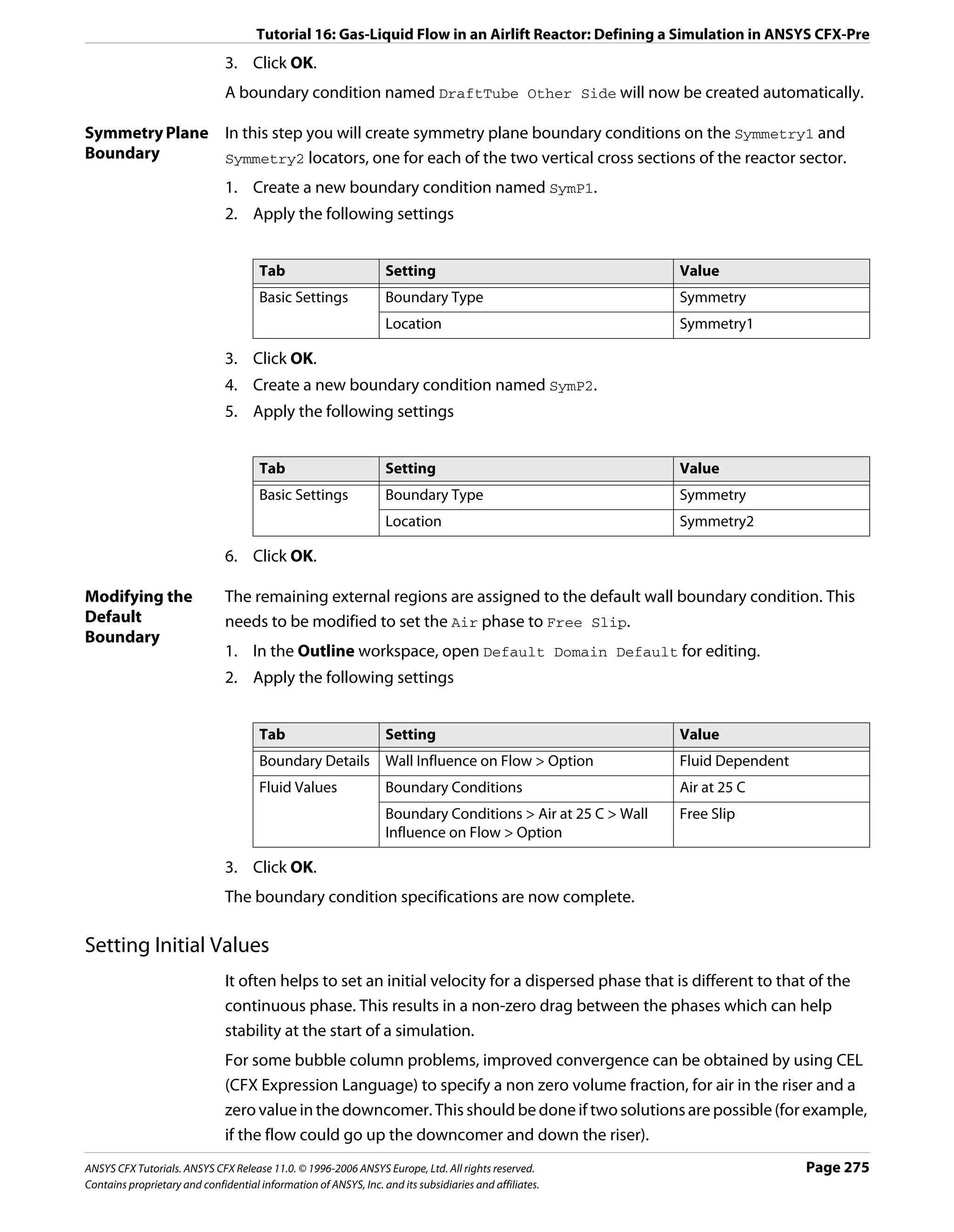
![Tutorial 16: Gas-Liquid Flow in an Airlift Reactor: Defining a Simulation in ANSYS CFX-Pre
1. Click Global Initialization .
Since a single pressure field exists for a multiphase calculation you do not set pressure
values on a per fluid basis.
2. Apply the following settings
Tab Setting Value
Fluid Settings Fluid Specific Initialization Air at 25 C
Fluid Specific Initialization > Air at 25 C (Selected)
Fluid Specific Initialization > Air at 25 C > Initial Automatic with Value
Conditions > Cartesian Velocity Components >
Option
Fluid Specific Initialization > Air at 25 C > Initial 0 [m s^-1]
Conditions > Cartesian Velocity Components > U
Fluid Specific Initialization > Air at 25 C > Initial 0.3 [m s^-1]
Conditions > Cartesian Velocity Components > V
Fluid Specific Initialization > Air at 25 C > Initial 0 [m s^-1]
Conditions > Cartesian Velocity Components > W
Fluid Specific Initialization Water*
Fluid Specific Initialization > Water (Selected)
Fluid Specific Initialization > Water > Initial Automatic with Value
Conditions > Cartesian Velocity Components >
Option
Fluid Specific Initialization > Water > Initial 0 [m s^-1]
Conditions > Cartesian Velocity Components > U
Fluid Specific Initialization > Water > Initial 0 [m s^-1]
Conditions > Cartesian Velocity Components > V
Fluid Specific Initialization > Water > Initial 0 [m s^-1]
Conditions > Cartesian Velocity Components > W
Fluid Specific Initialization > Water > Initial Automatic
Conditions > Turbulence Kinetic Energy > Option
Fluid Specific Initialization > Water > Initial (Selected)
Conditions > Turbulence Eddy Dissipation
Fluid Specific Initialization > Water > Initial Automatic
Conditions > Turbulence Eddy Dissipation >
Option
Fluid Specific Initialization > Water > Initial Automatic with Value
Conditions > Volume Fraction > Option
Fluid Specific Initialization > Water > Initial 1†
Conditions > Volume Fraction > Volume Fraction
*. Since there is no water entering or leaving the domain, a stationary initial guess is
recommended.
†. The volume fractions must sum to unity over all fluids. Since a value has been set for
water, the volume fraction of air will be calculated as the remaining difference, in
this case, 0.
3. Click OK.
Page 276 ANSYS CFX Tutorials. ANSYS CFX Release 11.0. © 1996-2006 ANSYS Europe, Ltd. All rights reserved.
Contains proprietary and confidential information of ANSYS, Inc. and its subsidiaries and affiliates.](https://image.slidesharecdn.com/ansys11tutorial-111218135319-phpapp01/75/Ansys-11-tutorial-288-2048.jpg)
![Tutorial 16: Gas-Liquid Flow in an Airlift Reactor: Obtaining a Solution using ANSYS CFX-Solver Manager
Setting Solver Control
If you are using a maximum edge length of 0.005 m or less to produce a finer mesh, use a
Target Residual of 1.0E-05 to obtain a more accurate solution.
1. Click Solver Control .
2. Apply the following settings
Tab Setting Value
Basic Settings Convergence Control > Fluid Timescale Physical Timescale
Control > Timescale Control
Convergence Control > Fluid Timescale 1 [s]
Control > Physical Timescale
3. Click OK.
Writing the Solver (.def) File
1. Click Write Solver File .
2. Apply the following settings:
Setting Value
File name BubbleColumn.def
Quit CFX–Pre* (Selected)
*. If using ANSYS CFX-Pre in Standalone Mode.
3. Ensure Start Solver Manager is selected and click Save.
4. If using Standalone Mode, quit ANSYS CFX-Pre, saving the simulation (.cfx) file at your
discretion.
Obtaining a Solution using ANSYS CFX-Solver Manager
The ANSYS CFX-Solver Manager will be launched after ANSYS CFX-Pre has closed down. You
will be able to obtain a solution to the CFD problem by following the instructions below.
Note: If a fine mesh is used for a formal quantitative analysis of the flow in the reactor, the
solution time will be significantly longer than for the coarse mesh. You can run the
simulation in parallel to reduce the solution time. For details, see Obtaining a Solution in
Parallel (p. 116).
1. Ensure Define Run is displayed.
2. Click Start Run.
ANSYS CFX-Solver runs and attempts to obtain a solution. This can take a long time
depending on your system. Eventually a dialog box is displayed stating that the
simulation has completed.
ANSYS CFX Tutorials. ANSYS CFX Release 11.0. © 1996-2006 ANSYS Europe, Ltd. All rights reserved. Page 277
Contains proprietary and confidential information of ANSYS, Inc. and its subsidiaries and affiliates.](https://image.slidesharecdn.com/ansys11tutorial-111218135319-phpapp01/75/Ansys-11-tutorial-289-2048.jpg)
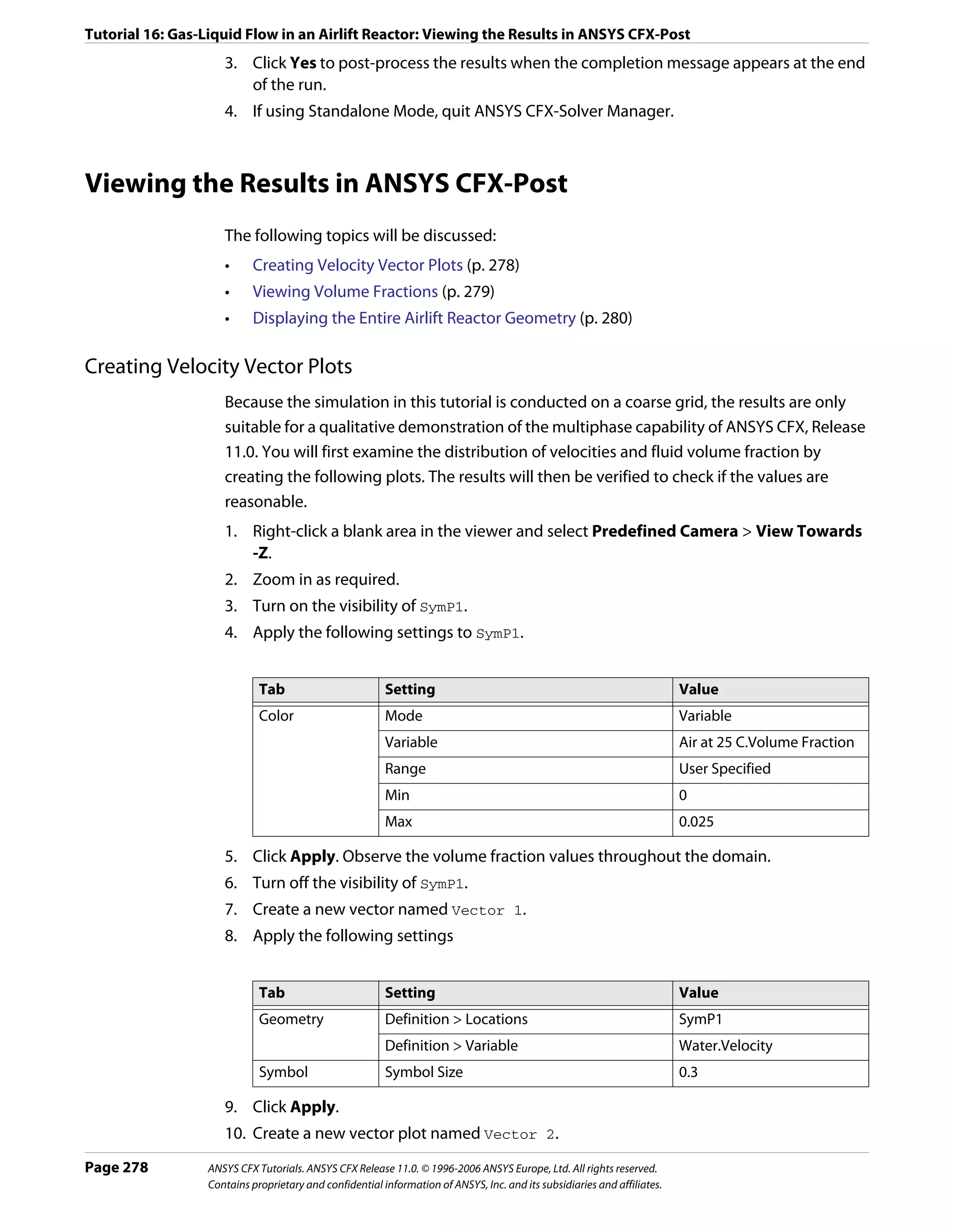
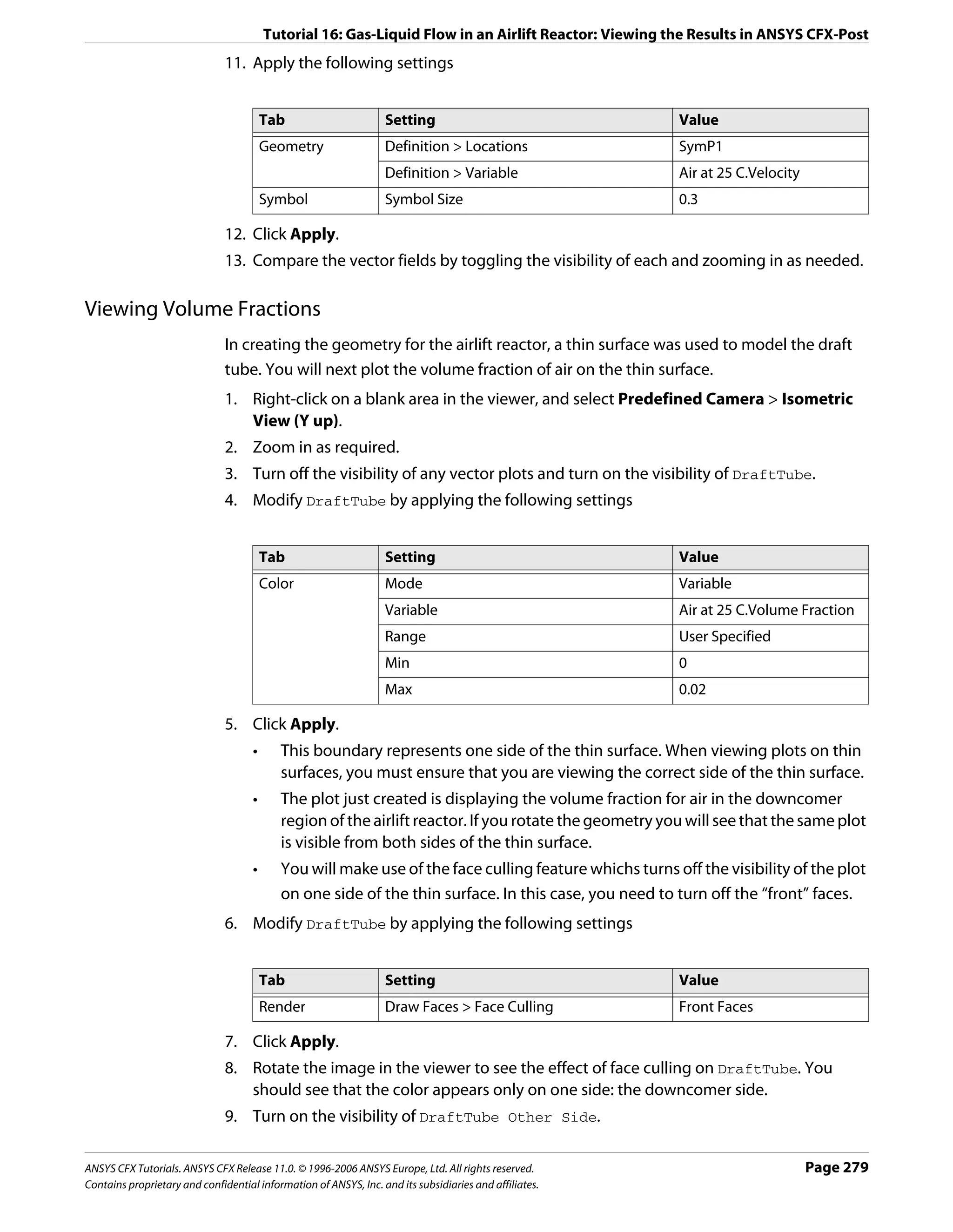
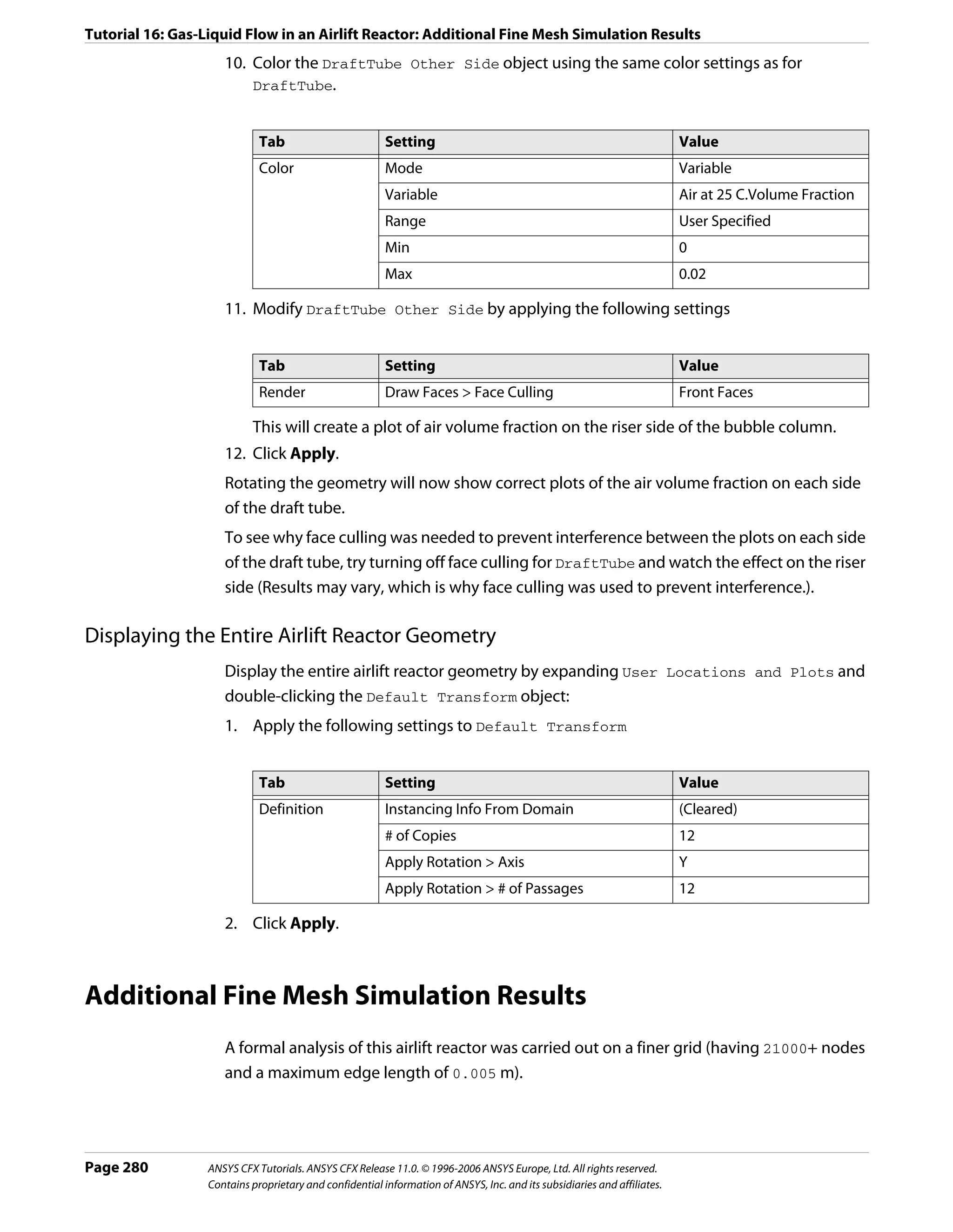


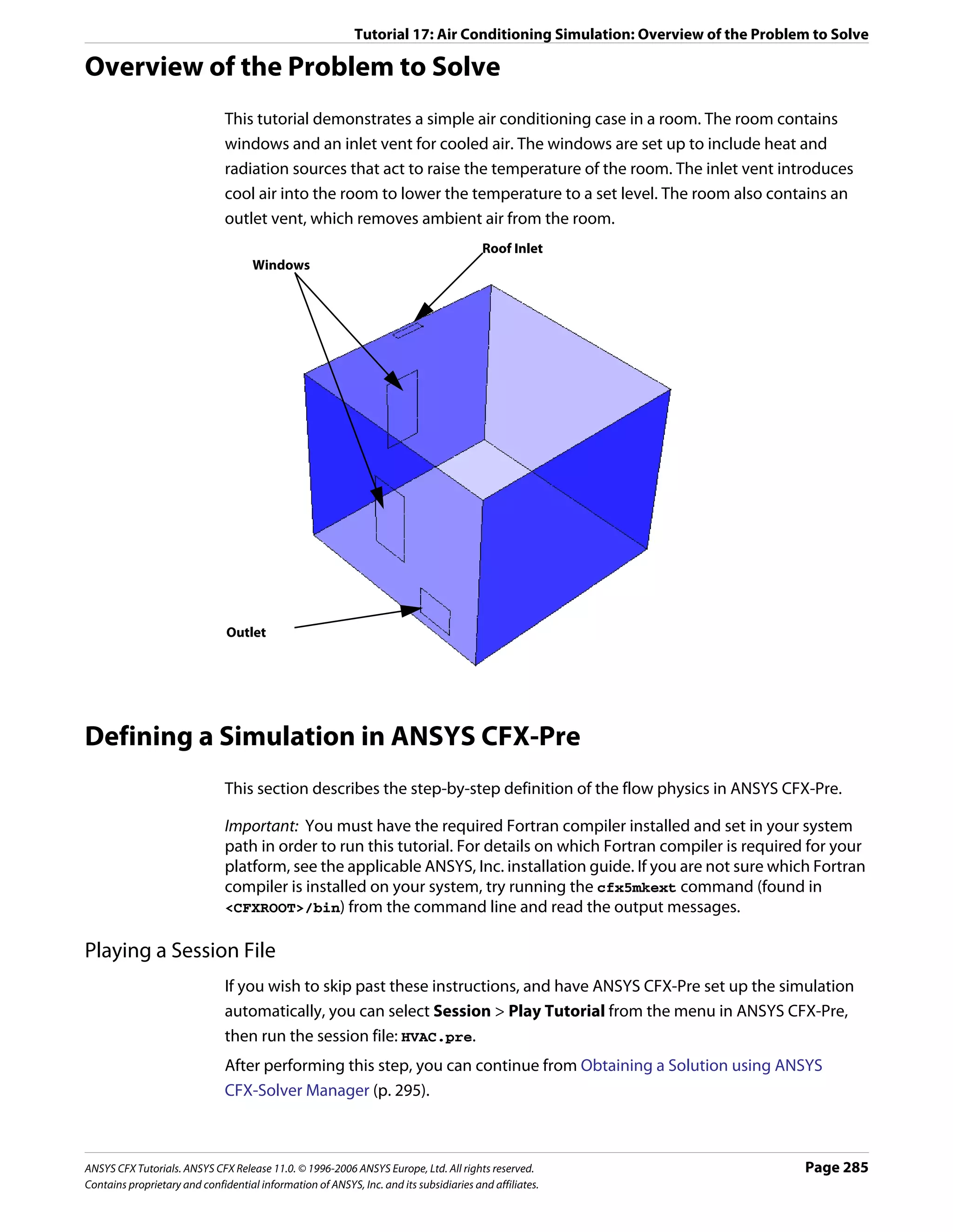

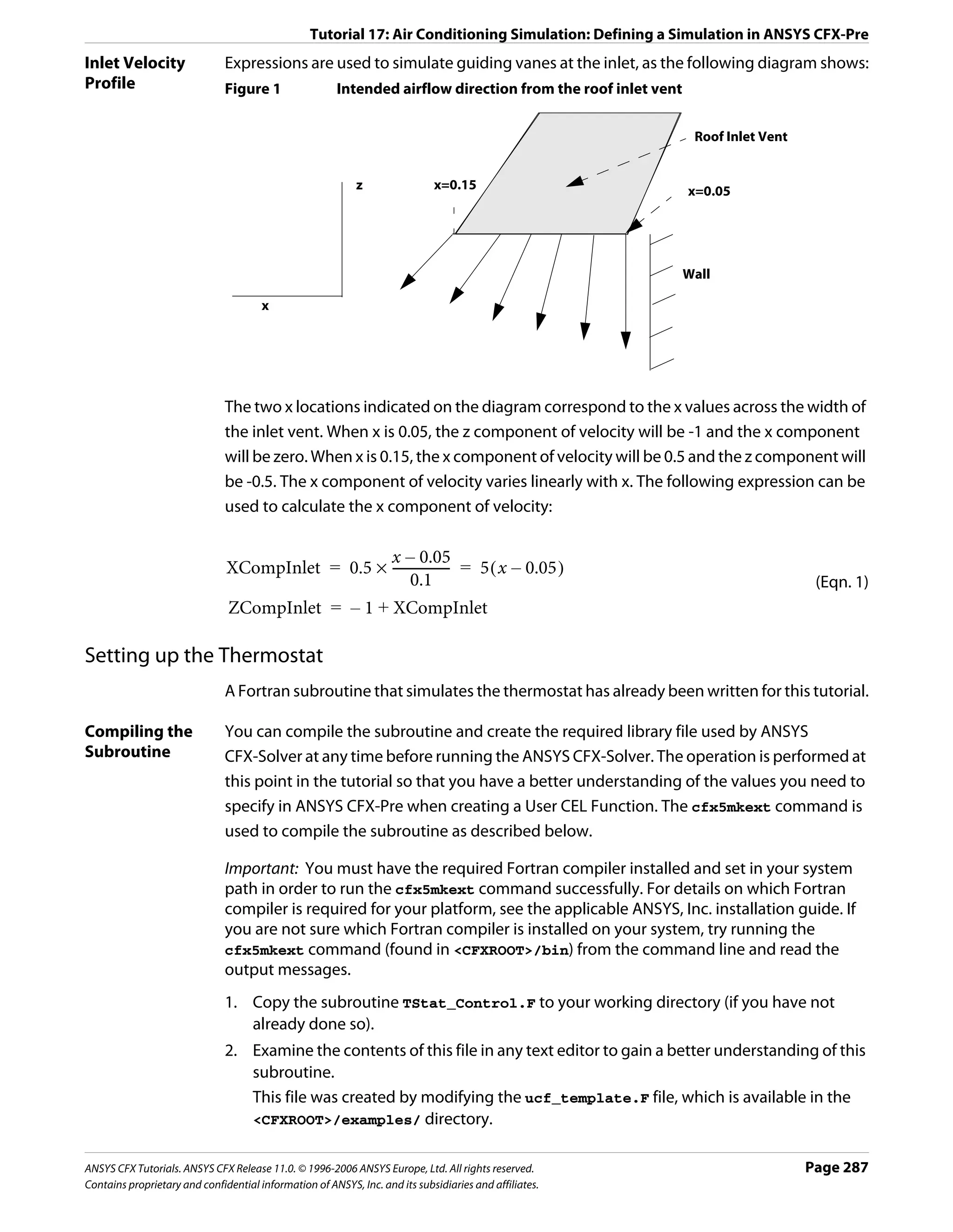
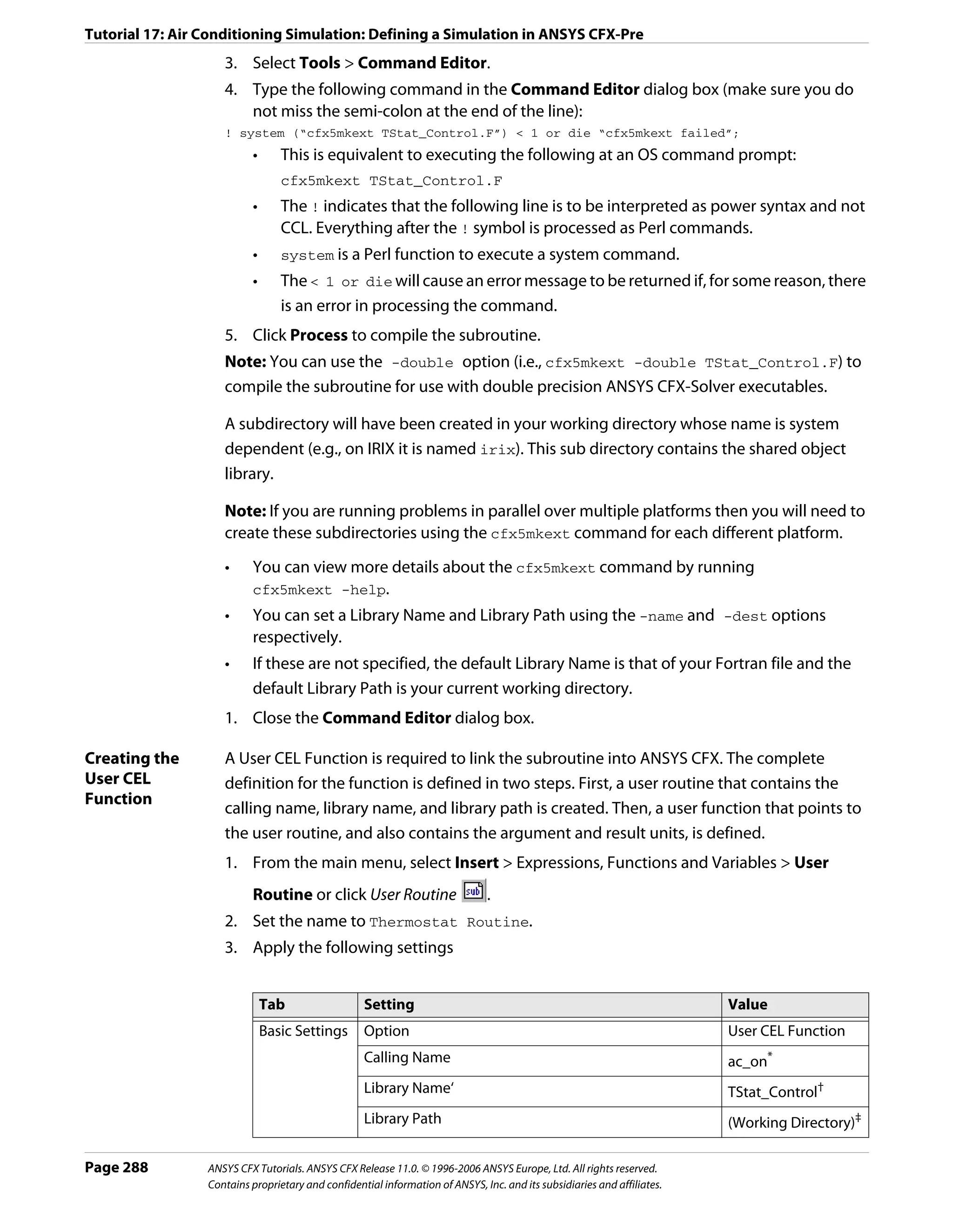
![Tutorial 17: Air Conditioning Simulation: Defining a Simulation in ANSYS CFX-Pre
*. This is the name of the subroutine within the Fortran file. Always use lower case
letters for the calling name, even if the subroutine name in the Fortran file is in
upper case.
†. This is the name passed to the cfx5mkext command by the -name option. If the
-name option is not specified, a default is used. The default is the Fortran file name
without the .F extension.
‡. Set this to your working directory.
4. Click OK.
5. Create a new user function named Thermostat Function by selecting Insert >
Expressions, Functions and Variables > User Function from the main menu.
6. Apply the following settings
Tab Setting Value
Basic Settings Option User Function
Argument Units [K], [K], [K], []*
Result Units []†
*. These are the units for the four input arguments: TSensor, TSet, TTol, and aitern.
†. The result will be a dimensionless integer flag of values 1 or 0.
7. Click OK.
The function you have just prepared is called during the evaluation of the expression for
ACOn (that you imported earlier). The expression is:
Thermostat Function(TSensor,TSet,TTol,aitern)
It evaluates to 1 or 0, depending on whether the air conditioner should be on (1) or off
(0).
Setting the Simulation Type
1. Click Simulation Type .
2. Apply the following settings
Tab Setting Value
Basic Settings Simulation Type > Option Transient
Simulation Type > Time Duration > Total Time tTotal
Simulation Type > Time Steps > Timesteps tStep
Simulation Type > Initial Time > Time 0 [s]
3. Click OK.
Creating the Domain
1. Right click Simulation in the Outline tree view and ensure that Automatic Default
Domain is selected. A domain named Default Domain should now appear under the
Simulation branch.
2. Double click Default Domain and apply the following settings:
ANSYS CFX Tutorials. ANSYS CFX Release 11.0. © 1996-2006 ANSYS Europe, Ltd. All rights reserved. Page 289
Contains proprietary and confidential information of ANSYS, Inc. and its subsidiaries and affiliates.](https://image.slidesharecdn.com/ansys11tutorial-111218135319-phpapp01/75/Ansys-11-tutorial-301-2048.jpg)
![Tutorial 17: Air Conditioning Simulation: Defining a Simulation in ANSYS CFX-Pre
Tab Setting Value
General Basic Settings > Location B1.P3
Options
Fluids List Air Ideal Gas
Domain Models > Pressure > Reference Pressure 1 [atm]
Domain Models > Buoyancy > Option Buoyant
Domain Models > Buoyancy > Gravity X Dirn. 0 [m s^-2]
Domain Models > Buoyancy > Gravity Y Dirn. 0 [m s^-2]
Domain Models > Buoyancy > Gravity Z Dirn. -g
Domain Models > Buoyancy > Buoy. Ref. Density 1.2 [kg m^-3]
Fluid Models Heat Transfer > Option Thermal Energy
Thermal Radiation Model > Option Monte Carlo
3. Click OK.
Setting Boundary Conditions
In this section you will define the locations and values of the boundary conditions.
Inlet Boundary 1. Create a new boundary condition named Inlet.
2. Apply the following settings
Tab Setting Value
Basic Settings Boundary Type Inlet
Location Inlet
Boundary Details Mass and Momentum > Option Mass Flow Rate
Mass and Momentum > Mass Flow Rate MassFlow
Flow Direction > Option Cartesian Components
Flow Direction > X Component XCompInlet
Flow Direction > Y Component 0
Flow Direction > Z Component ZCompInlet
Heat Transfer > Static Temperature TIn
Plot Options Boundary Vector (Selected)
3. Click OK.
Note: Ignore the physics errors that appear. They will be fixed by setting up the rest of the
simulation. The error you see is due to a reference to Thermometer which has not been set
up yet. This will be done as part of the output control.
Outlet 1. Create a new boundary condition named VentOut.
Boundary 2. Apply the following settings
Page 290 ANSYS CFX Tutorials. ANSYS CFX Release 11.0. © 1996-2006 ANSYS Europe, Ltd. All rights reserved.
Contains proprietary and confidential information of ANSYS, Inc. and its subsidiaries and affiliates.](https://image.slidesharecdn.com/ansys11tutorial-111218135319-phpapp01/75/Ansys-11-tutorial-302-2048.jpg)
![Tutorial 17: Air Conditioning Simulation: Defining a Simulation in ANSYS CFX-Pre
Tab Setting Value
Basic Settings Boundary Type Outlet
Location VentOut
Boundary Details Mass and Momentum > Relative Pressure 0 [Pa]
3. Click OK.
Window To model incoming radiation at the window boundaries, a directional radiation source will
Boundary be created. The windows will also contribute heat to the room via a fixed temperature of
26 [C].
1. Create a new boundary condition named Windows.
2. Apply the following settings
Tab Setting Value
Basic Boundary Type Wall
Settings Location Window1, Window2
Boundary Heat Transfer > Option Temperature
Details Heat Transfer > Fixed Temperature 26 [C]
3. Apply the following settings
Tab Setting Value
Sources Boundary Source (Selected)
Boundary Source > Sources (Selected)
4. Create a new radiation source item by clicking Add New Item and accepting the
default name.
5. Apply the following settings to Radiation Source 1
Setting Value
Option Directional Radiation Flux
Radiation Flux 600 [W m^-2]
Direction > Option Cartesian Components
Direction > X Component 0.33
Direction > Y Component 0.33
Direction > Z Component -0.33
6. Apply the following setting
Tab Setting Value
Plot Boundary Vector (Selected)
Options
ANSYS CFX Tutorials. ANSYS CFX Release 11.0. © 1996-2006 ANSYS Europe, Ltd. All rights reserved. Page 291
Contains proprietary and confidential information of ANSYS, Inc. and its subsidiaries and affiliates.](https://image.slidesharecdn.com/ansys11tutorial-111218135319-phpapp01/75/Ansys-11-tutorial-303-2048.jpg)
![Tutorial 17: Air Conditioning Simulation: Defining a Simulation in ANSYS CFX-Pre
7. Click OK.
The directional source of radiation is displayed.
Default Wall The default boundary condition for any undefined surface in ANSYS CFX-Pre is a no-slip,
Boundary smooth, adiabatic wall. For radiation purposes, the default wall is assumed to be a perfectly
absorbing and emitting surface (emissivity = 1), and this will be preserved when setting up
the boundary condition.
In this tutorial, a fixed temperature of 26 °C will be assumed to exist at the wall during the
simulation. A more detailed analysis would model heat transfer through the walls, but as
this tutorial is designed only for demonstration purposes, a fixed temperature wall is
sufficient.
1. Modify the boundary condition named Default Domain Default.
2. Apply the following settings
Tab Setting Value
Boundary Heat Transfer > Option Temperature
Details Heat Transfer > Fixed Temperature 26 [C]
3. Click OK.
This setting will include the Door region, which will be modeled as a wall (closed door) for
simplicity. Since the region is part of the entire default boundary, it will not appear in the
wireframe when the results file is opened in ANSYS CFX-Post (but can still be viewed in the
Regions list).
Setting Initial Values
1. Click Global Initialization .
2. Apply the following settings
Page 292 ANSYS CFX Tutorials. ANSYS CFX Release 11.0. © 1996-2006 ANSYS Europe, Ltd. All rights reserved.
Contains proprietary and confidential information of ANSYS, Inc. and its subsidiaries and affiliates.](https://image.slidesharecdn.com/ansys11tutorial-111218135319-phpapp01/75/Ansys-11-tutorial-304-2048.jpg)
![Tutorial 17: Air Conditioning Simulation: Defining a Simulation in ANSYS CFX-Pre
Tab Setting Value
Global Settings Initial Conditions > Velocity Type Cartesian
Initial Conditions > Cartesian Velocity Automatic with Value
Components > Option
Initial Conditions > Cartesian Velocity 0 [m s^-1]
Components > U
Initial Conditions > Cartesian Velocity 0 [m s^-1]
Components > V
Initial Conditions > Cartesian Velocity 0 [m s^-1]
Components > W
Initial Conditions > Static Pressure > Relative 0 [Pa]
Pressure
Initial Conditions > Temperature > Temperature 22 [C]
Initial Conditions > Turbulence Kinetic Energy > (Selected)
Fractional Intensity
Initial Conditions > Turbulence Eddy Dissipation (Selected)
Initial Conditions > Turbulence Eddy Dissipation (Selected)
> Eddy Length Scale
Initial Conditions > Turbulence Eddy Dissipation 0.25 [m]
> Eddy Length Scale > Eddy Len. Scale
Initial Conditions > Radiation Intensity > (Selected)
Blackbody Temperature
Initial Conditions > Radiation Intensity > 22 [C]
Blackbody Temperature > Blackbody Temp.
3. Click OK.
Setting Solver Control
1. Click Solver Control .
2. Apply the following settings
Tab Setting Value
Basic Settings Transient Scheme > Option Second Order Backward
Euler
Convergence Control > Max. Coeff. Loops 3
3. Click OK.
Setting Output Control
Transient results files will be set up to record transient values of a chosen set of variables.
Monitor points will be created to show the on/off status of the air conditioner, the
temperature at the inlet, the temperature at the outlet, and the temperature at a prescribed
thermometer location.
ANSYS CFX Tutorials. ANSYS CFX Release 11.0. © 1996-2006 ANSYS Europe, Ltd. All rights reserved. Page 293
Contains proprietary and confidential information of ANSYS, Inc. and its subsidiaries and affiliates.](https://image.slidesharecdn.com/ansys11tutorial-111218135319-phpapp01/75/Ansys-11-tutorial-305-2048.jpg)
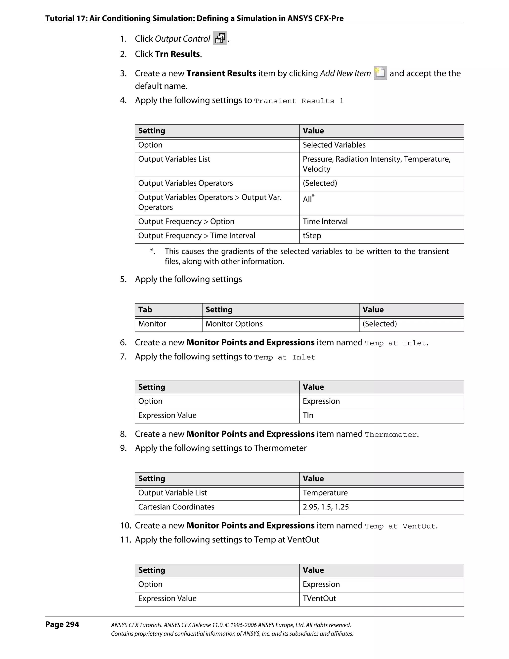
![Tutorial 17: Air Conditioning Simulation: Viewing the Results in ANSYS CFX-Post
Creating Graphics Objects
Plane locators will be placed vertically through the vents and horizontally above the floor.
Plane Locators 1. Load the res file (HVAC_001.res) if you did not elect to load the results directly from the
ANSYS CFX-Solver Manager.
2. Right-click a blank area in the viewer, select Predefined Camera > Isometric View (Z
up).
3. Create a ZX-Plane named Plane 1 with Y=1.5 [m]. Color it by Temperature using a
user specified range from 19 [C] to 23 [C], and clear Lighting.
4. Create an XY Plane named Plane 2 with Z=0.35 [m]. Color it using the same settings
as for the first plane, and clear Lighting.
Isosurface 1. Click Timestep Selector .
Locator The Timestep Selector appears.
2. Double-click the value (12s) in the Timestep Selector.
The Timestep is set to 12s so that the cold plume is visible.
3. Create an isosurface named Cold Plume which is a surface of Temperature=19 [C].
Use conservative values for Temperature.
4. Color the isosurface by Temperature and use the same range as for the planes.
Although the color of the isosurface will not show variation (by definition), it will be
consistent with the other graphic objects.
5. On the Render tab for the isosurface, set Transparency to 0.5, and clear Lighting.
6. Click Apply.
Note: The isosurface will not be visible in some timesteps, but you will be able to see it when
playing the animation (a step carried out later).
Adjusting the The legend title should not name the locator of any particular object since all objects are
Legend colored by the same variable and use the same range.
1. In the tree view, double-click Default Legend View 1.
2. In the Definition tab, change Title Mode to Variable.
This will remove the locator name from the legend.
3. Click the Appearance tab, then:
a. Change Precision to 2, Fixed.
b. Change Text Height to 0.03.
4. Click Apply.
A label will be used to show the simulation time and the temperature of the thermometer
which controls the thermostat. This will be especially useful for the animation which is
created later in this tutorial.
Page 296 ANSYS CFX Tutorials. ANSYS CFX Release 11.0. © 1996-2006 ANSYS Europe, Ltd. All rights reserved.
Contains proprietary and confidential information of ANSYS, Inc. and its subsidiaries and affiliates.](https://image.slidesharecdn.com/ansys11tutorial-111218135319-phpapp01/75/Ansys-11-tutorial-308-2048.jpg)


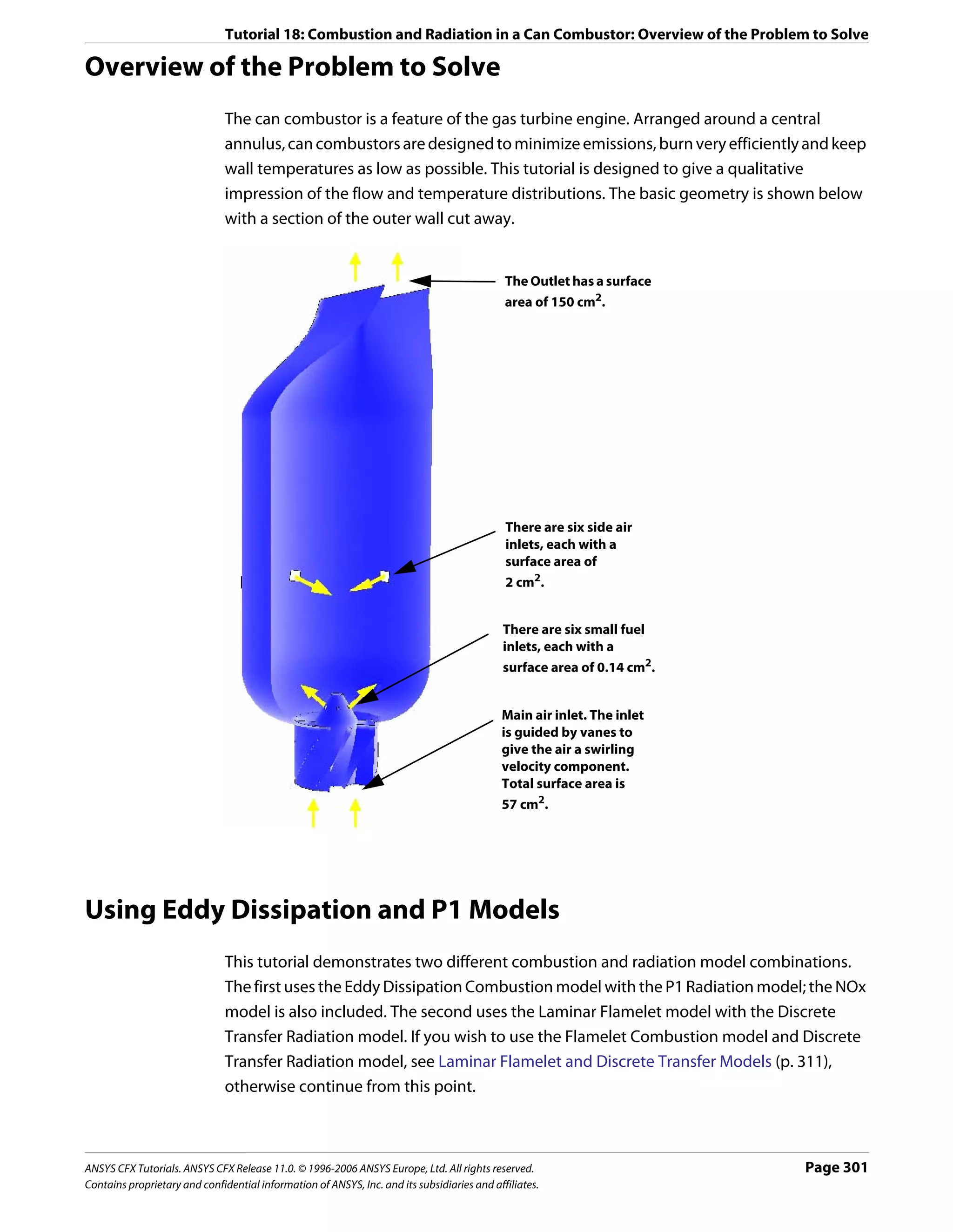
![Tutorial 18: Combustion and Radiation in a Can Combustor: Defining a Simulation in ANSYS CFX-Pre
Tab Setting Value
Mixture Mixture Properties (Selected)
Properties Mixture Properties > Radiation Properties > (Selected)†
Refractive Index
Mixture Properties > Radiation Properties > (Selected)
Absorption Coefficient
Mixture Properties > Radiation Properties > (Selected)
Scattering Coefficient
*. The Methane Air WD1 NO PDF reaction specifies complete combustion of the fuel
into its products in a single-step reaction. The formation of NO is also modeled and
occurs in an additional reaction step.
Click to display the Reactions List dialog box, then click Import Library Data
and select the appropriate reaction to import.
†. Setting the radiation properties explicitly will significantly shorten the solution time
since the ANSYS CFX-Solver will not have to calculate radiation mixture properties.
3. Click OK.
Creating the Domain
1. Right click Simulation in the Outline tree view and ensure that Automatic Default
Domain is selected. A domain named Default Domain should now appear under the
Simulation branch.
2. Double click Default Domain and apply the following settings
Tab Setting Value
General Basic Settings > Locations B152, B153, B154,
Options B155, B156
Basic Settings > Fluids List Methane Air Mixture
Domain Models > Pressure > Reference Pressure 1 [atm]*
Fluid Models Heat Transfer > Option Thermal Energy
Reaction or Combustion > Option Eddy Dissipation
Reaction or Combustion > Eddy Dissipation Model (Selected)
Coefficient B
Reaction or Combustion > Eddy Dissipation Model 0.5†
Coefficient B > EDM Coeff. B
Thermal Radiation Model > Option P1
Component Details > N2 (Selected)
Component Details > N2 > Option Constraint
*. It is important to set a realistic reference pressure in this tutorial because the
components of Methane Air Mixture are ideal gases.
†. This includes a simple model for partial premixing effects by turning on the Product
Limiter. When it is selected, non-zero initial values are required for the products. The
products limiter is not recommended for multi-step eddy dissipation reactions, and
so is set for this single step reaction only.
3. Click OK.
ANSYS CFX Tutorials. ANSYS CFX Release 11.0. © 1996-2006 ANSYS Europe, Ltd. All rights reserved. Page 303
Contains proprietary and confidential information of ANSYS, Inc. and its subsidiaries and affiliates.](https://image.slidesharecdn.com/ansys11tutorial-111218135319-phpapp01/75/Ansys-11-tutorial-315-2048.jpg)
![Tutorial 18: Combustion and Radiation in a Can Combustor: Defining a Simulation in ANSYS CFX-Pre
Creating the Boundary Conditions
Fuel Inlet 1. Create a new boundary condition named fuelin.
Boundary 2. Apply the following settings
Tab Setting Value
Basic Settings Boundary Type Inlet
Location fuelin
Boundary Details Mass and Momentum > Normal Speed 40 [m s^-1]
Heat Transfer > Static Temperature 300 [K]
Component Details CH4
Component Details > CH4 > Mass Fraction 1
3. Click OK.
Bottom Air Inlet Two separate boundary conditions will be applied for the incoming air. The first is at the
Boundary base of the can combustor. The can combustor employs vanes downstream of the fuel inlet
to give the incoming air a swirling velocity.
1. Create a new boundary condition named airin.
2. Apply the following settings
Tab Setting Value
Basic Settings Boundary Type Inlet
Location airin
Boundary Details Mass and Momentum > Normal Speed 10 [m s^-1]
Heat Transfer > Static Temperature 300 [K]
Component Details O2
Component Details > O2 > Mass Fraction 0.232*
*. The remaining mass fraction at the inlet will be made up from the constraint
component, N2.
3. Click OK.
Side Air Inlet The secondary air inlets are located on the side of the vessel and introduce extra air to aid
Boundary combustion.
1. Create a new boundary condition named secairin.
2. Apply the following settings
Tab Setting Value
Basic Settings Boundary Type Inlet
Location secairin
Page 304 ANSYS CFX Tutorials. ANSYS CFX Release 11.0. © 1996-2006 ANSYS Europe, Ltd. All rights reserved.
Contains proprietary and confidential information of ANSYS, Inc. and its subsidiaries and affiliates.](https://image.slidesharecdn.com/ansys11tutorial-111218135319-phpapp01/75/Ansys-11-tutorial-316-2048.jpg)
![Tutorial 18: Combustion and Radiation in a Can Combustor: Defining a Simulation in ANSYS CFX-Pre
Tab Setting Value
Boundary Details Mass and Momentum > Option Normal Speed
Mass and Momentum > Normal Speed 6 [m s^-1]
Heat Transfer > Option Static Temperature
Heat Transfer > Static Temperature 300 [K]
Component Details O2
Component Details > O2 > Mass Fraction 0.232*
*. The remaining mass fraction at the inlet will be made up from the constraint
component, N2.
3. Click OK.
Outlet 1. Create a new boundary condition named out.
Boundary 2. Apply the following settings
Tab Setting Value
Basic Settings Boundary Type Outlet
Location out
Boundary Details Mass and Momentum > Option Average Static Pressure
Mass and Momentum > Relative Pressure 0 [Pa]
3. Click OK.
Vanes Boundary The vanes above the main air inlet are to be modeled as thin surfaces. To create a vane as a
thin surface in ANSYS CFX-Pre, you must specify a wall boundary condition on each side of
the vanes. The Create Thin Surface Partner feature in ANSYS CFX-Pre will automatically
match the other side of a thin surface if you pick just a single side.
You will first create a new region which contains one side of each of the eight vanes, then
use the Create Thin Surface Partner feature to match the other side.
1. Create a new composite region named Vane Surfaces.
2. Apply the following settings
Tab Setting Value
Basic Settings Dimension (Filter) 2D*
Region List F129.152, F132.152, F136.152,
F138.152, F141.152, F145.152,
F147.152, F150.152
*. This will filter out the 3D regions, leaving only 2D regions
3. Click OK.
4. Create a new boundary condition named vanes.
5. Apply the following settings
ANSYS CFX Tutorials. ANSYS CFX Release 11.0. © 1996-2006 ANSYS Europe, Ltd. All rights reserved. Page 305
Contains proprietary and confidential information of ANSYS, Inc. and its subsidiaries and affiliates.](https://image.slidesharecdn.com/ansys11tutorial-111218135319-phpapp01/75/Ansys-11-tutorial-317-2048.jpg)
![Tutorial 18: Combustion and Radiation in a Can Combustor: Defining a Simulation in ANSYS CFX-Pre
Tab Setting Value
Basic Settings Boundary Type Wall
Location Vane Surfaces
Create Thin Surface Partner (Selected)*
*. This feature will attempt to match all primitives specified in the location list to
create a thin surface boundary condition.
6. Click OK.
Default Wall The default boundary condition for any undefined surface in ANSYS CFX-Pre is a no-slip,
Boundary smooth, adiabatic wall.
• For radiation purposes, the wall is assumed to be a perfectly absorbing and emitting
surface (emissivity = 1).
• The wall is non-catalytic, i.e., it does not take part in the reaction.
Since this tutorial serves as a basic model, heat transfer through the wall is neglected. As a
result, no further boundary conditions need to be defined.
Setting Initial Values
1. Click Global Initialization .
2. Apply the following settings
Tab Setting Value
Global Initial Conditions > Cartesian Velocity Components > Automatic with Value
Settings Option
Initial Conditions > Cartesian Velocity Components > U 0 [m s^-1]
Initial Conditions > Cartesian Velocity Components > V 0 [m s^-1]
Initial Conditions > Cartesian Velocity Components > W 5 [m s^-1]
Initial Conditions > Turbulence Eddy Dissipation (Selected)
Initial Conditions > Turbulence Eddy Dissipation > Automatic
Option
Initial Conditions > Component Details O2
Initial Conditions > Component Details > O2> Option Automatic with Value
Initial Conditions > Component Details > O2 > Mass 0.232*
Fraction
Initial Conditions > Component Details CO2
Initial Conditions > Component Details > CO2 > Option Automatic with Value
Initial Conditions > Component Details > CO2 > Mass 0.01
Fraction
Initial Conditions > Component Details H2O
Initial Conditions > Component Details> H2O > Option Automatic with Value
Initial Conditions > Component Details > H2O > Mass 0.01
Fraction
Page 306 ANSYS CFX Tutorials. ANSYS CFX Release 11.0. © 1996-2006 ANSYS Europe, Ltd. All rights reserved.
Contains proprietary and confidential information of ANSYS, Inc. and its subsidiaries and affiliates.](https://image.slidesharecdn.com/ansys11tutorial-111218135319-phpapp01/75/Ansys-11-tutorial-318-2048.jpg)
![Tutorial 18: Combustion and Radiation in a Can Combustor: Obtaining a Solution using ANSYS CFX-Solver Manager
*. The initial conditions assume the domain consists mainly of air and the fraction of
oxygen in air is 0.232. A small mass fraction of reaction products (CO2 and H2O) is
needed for the EDM model to initiate combustion.
3. Click OK.
Setting Solver Control
1. Click Solver Control .
2. Apply the following settings
Tab Setting Value
Basic Settings Convergence Control > Max. Iterations 100
Convergence Control > Fluid Timescale Control > Physical Timescale
Timescale Control
Convergence Control > Fluid Timescale Control > 0.025 [s]
Physical Timescale
3. Click OK.
Writing the Solver (.def) File
1. Click Write Solver File .
2. Apply the following settings:
Setting Value
File name CombustorEDM.def
Quit CFX–Pre* (Selected)
*. If using ANSYS CFX-Pre in Standalone Mode.
3. Ensure Start Solver Manager is selected and click Save.
4. If using Standalone Mode, quit ANSYS CFX-Pre, saving the simulation (.cfx) file.
Obtaining a Solution using ANSYS CFX-Solver Manager
The ANSYS CFX-Solver Manager will be launched after ANSYS CFX-Pre saves the definition
file. You will be able to obtain a solution to the CFD problem by following the instructions
below.
Note: If a fine mesh is used for a formal quantitative analysis of the flow in the combustor,
the solution time will be significantly longer than for the coarse mesh. You can run the
simulation in parallel to reduce the solution time. For details, see Obtaining a Solution in
Parallel (p. 116).
1. Ensure Define Run is displayed.
Definition File should be set to CombustorEDM.def.
ANSYS CFX Tutorials. ANSYS CFX Release 11.0. © 1996-2006 ANSYS Europe, Ltd. All rights reserved. Page 307
Contains proprietary and confidential information of ANSYS, Inc. and its subsidiaries and affiliates.](https://image.slidesharecdn.com/ansys11tutorial-111218135319-phpapp01/75/Ansys-11-tutorial-319-2048.jpg)

![Tutorial 18: Combustion and Radiation in a Can Combustor: Viewing the Results in ANSYS CFX-Post
3. Create a new vector named Vector 1.
4. Apply the following settings
Tab Setting Value
Geometry Definition > Locations Plane 1
Symbol Symbol Size 2
5. Click Apply.
6. Create a new plane named Plane 2.
7. Apply the following settings
Tab Setting Value
Geometry Definition > Method XY Plane
Definition > Z 0.03
Plane Bounds > Type Rectangular
Plane Bounds > X Size 0.5 [m]
Plane Bounds > Y Size 0.5 [m]
Plane Type > Sample (Selected)
Plane Type > X Samples 30
Plane Type > Y Samples 30
Render Draw Faces (Cleared)
8. Click Apply.
9. Modify Vector 1.
10. Apply the following setting
Tab Setting Value
Geometry Definition > Locations Plane 2
11. Click Apply.
To view the swirling velocity field, right-click in the viewer and select Predefined Camera >
View Towards -Z.
You may also want to turn off the wireframe visibility. In the region near the fuel and air
inlets, the swirl component of momentum (theta direction) results in increased mixing with
the surrounding fluid and a higher residence time in this region. As a result, more fuel is
burned.
Viewing Radiation
Try examining the distribution of Incident Radiation and Radiation Intensity
throughout the domain.
When you are finished, quit ANSYS CFX-Post.
Page 310 ANSYS CFX Tutorials. ANSYS CFX Release 11.0. © 1996-2006 ANSYS Europe, Ltd. All rights reserved.
Contains proprietary and confidential information of ANSYS, Inc. and its subsidiaries and affiliates.](https://image.slidesharecdn.com/ansys11tutorial-111218135319-phpapp01/75/Ansys-11-tutorial-322-2048.jpg)
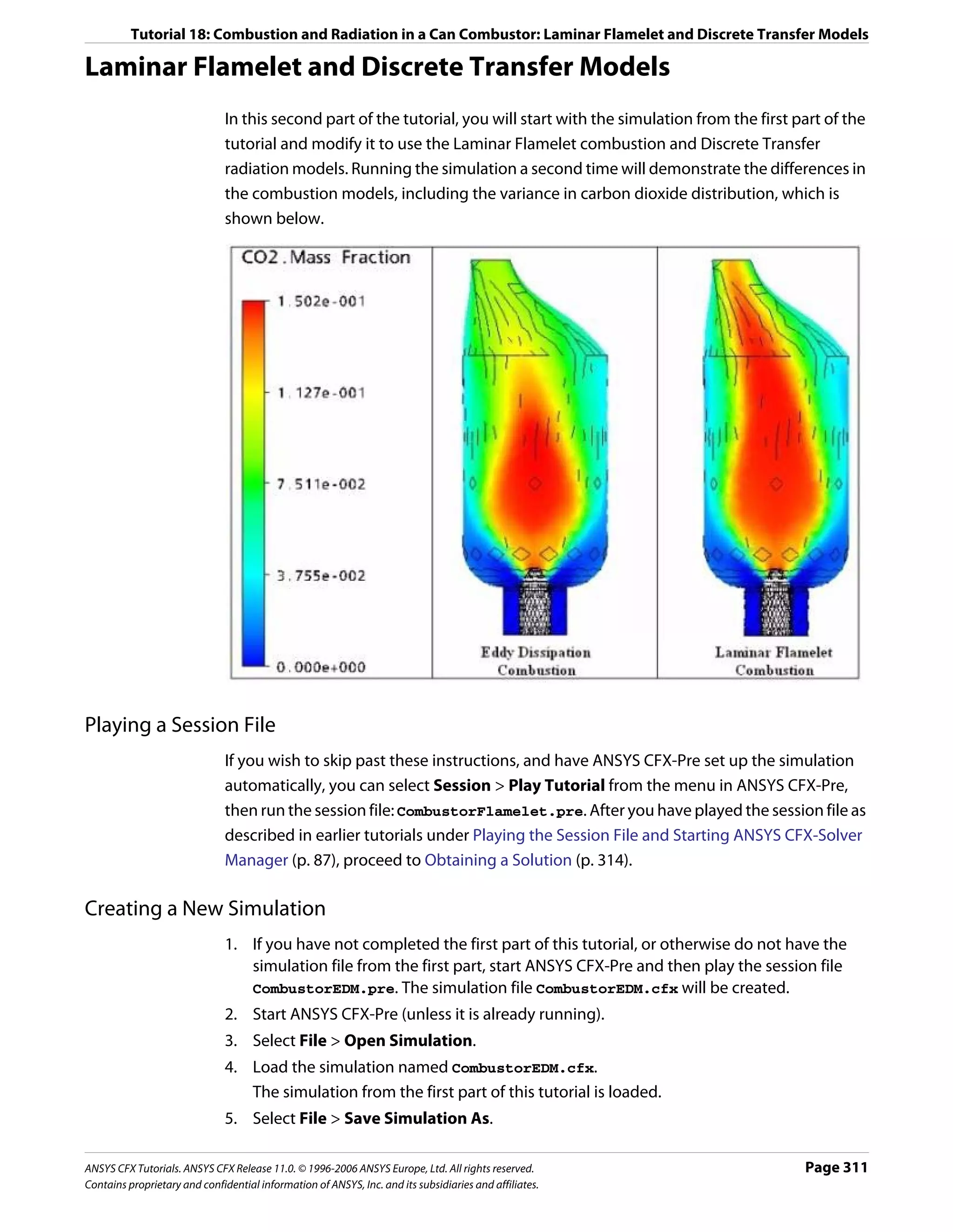
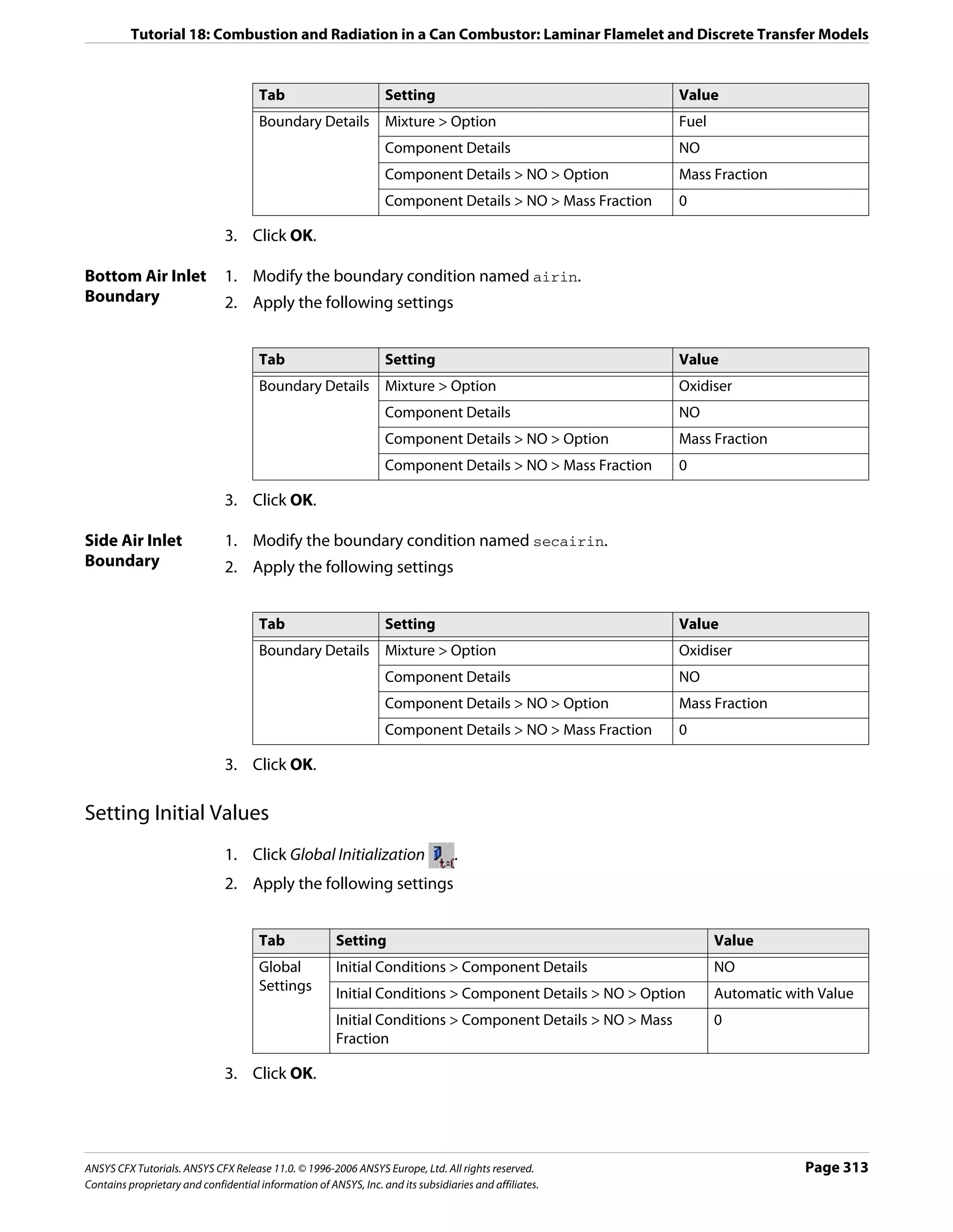
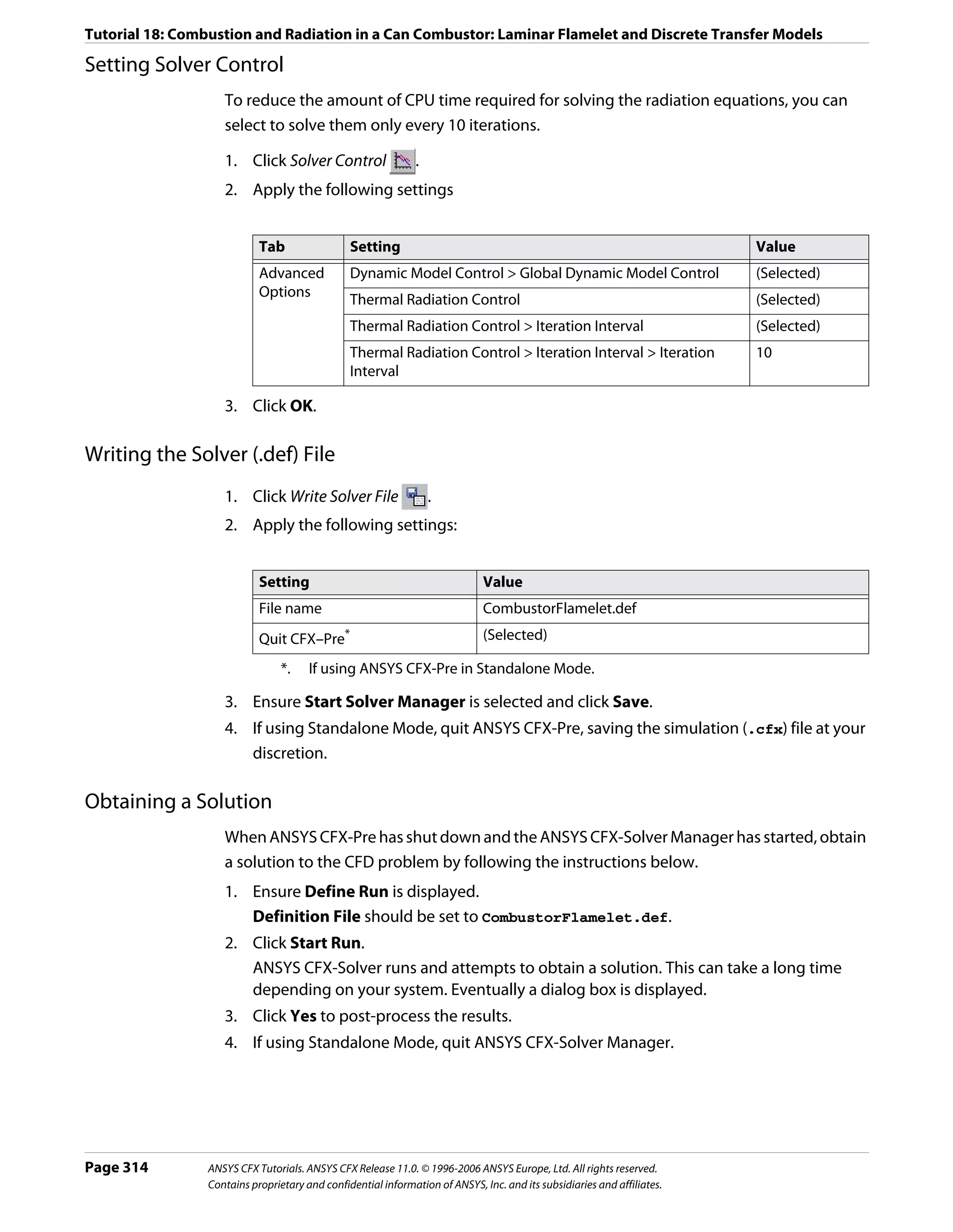
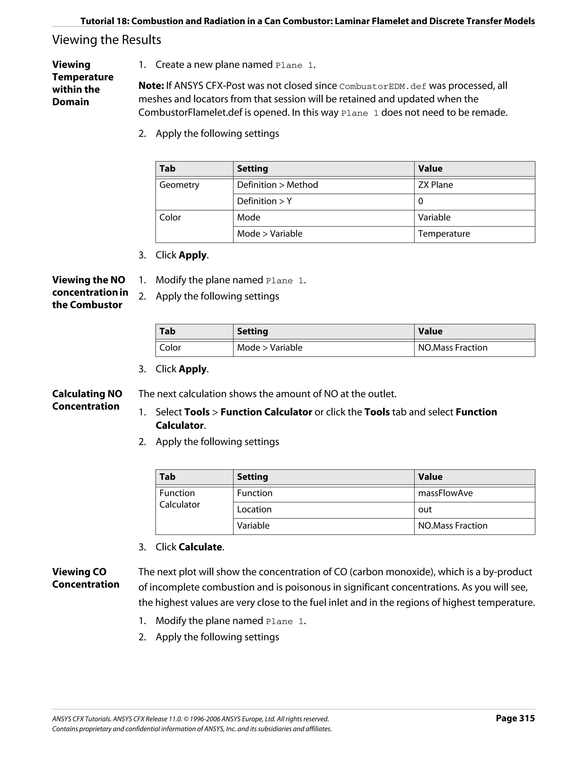

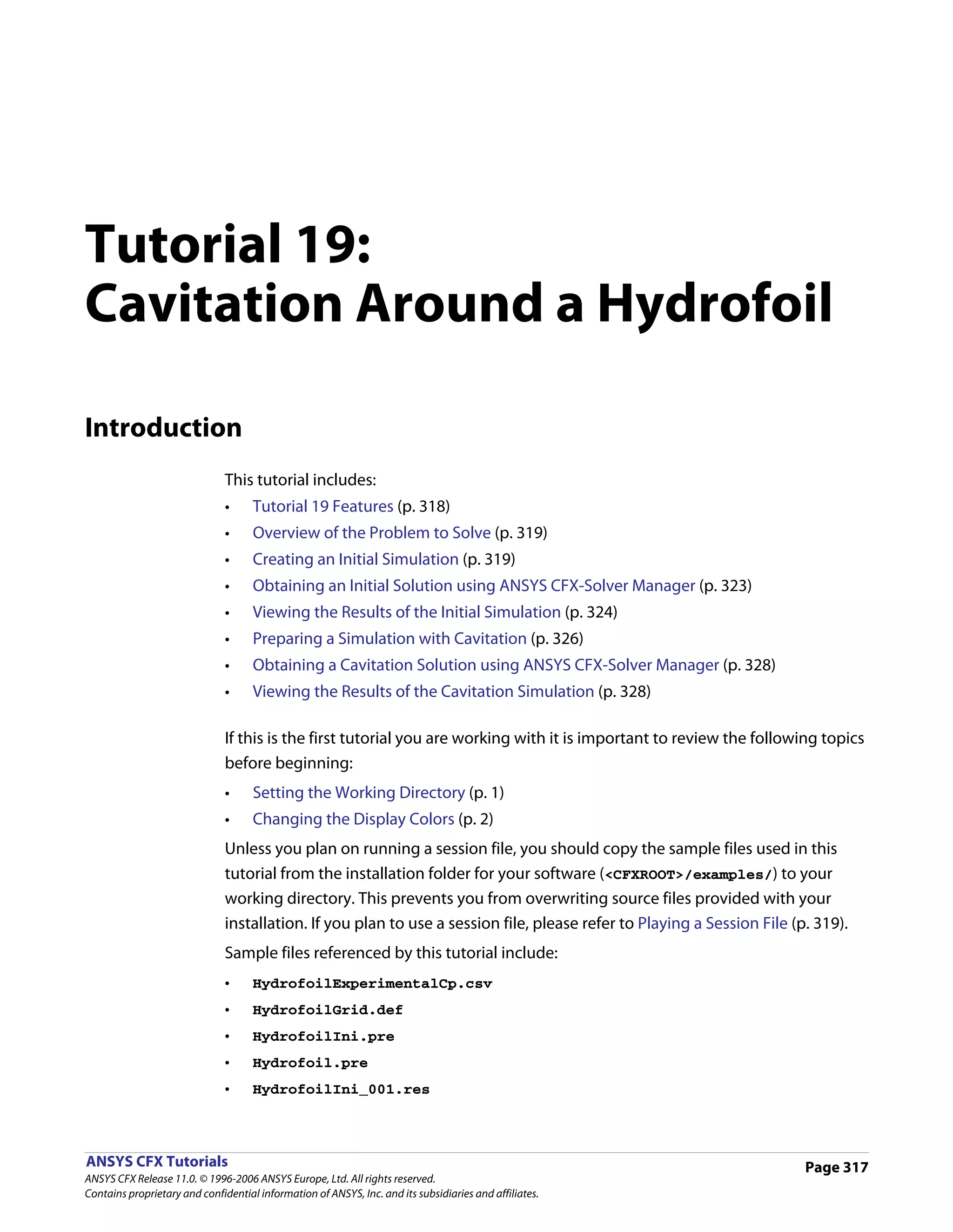

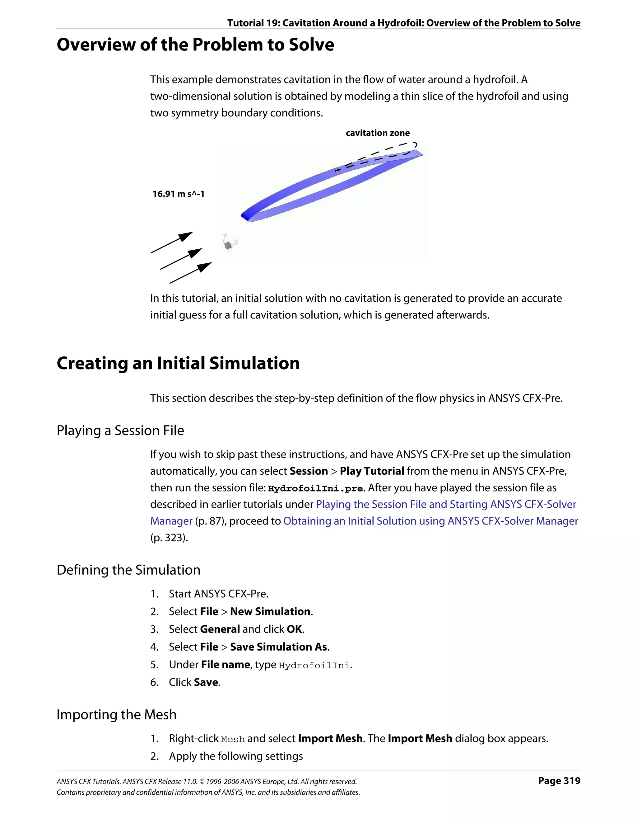
![Tutorial 19: Cavitation Around a Hydrofoil: Creating an Initial Simulation
Setting Value
File type CFX-Solver (*.def, *.ref, *.trn, *.bak)
File name HydrofoilGrid.def
3. Click Open.
4. Right-click a blank area in the viewer and select Predefined Camera > View Towards
-Z.
Loading Materials
Since this tutorial uses Water Vapour at 25 C and Water at 25 C you need to load these
materials.
1. In the Outline tree view, right-click Materials and select Import Library Data.
The Select Library Data to Import dialog box is displayed.
2. Expand Water Data.
3. Select both Water Vapour at 25 C and Water at 25 C by holding <Crtl> when
selecting.
4. Click OK.
Creating the Domain
The fluid domain used for this simulation contains liquid water and water vapour. The
volume fractions are initially set so that the domain is filled entirely with liquid.
1. Right click Simulation in the Outline tree view and ensure that Automatic Default
Domain is selected. A domain named Default Domain should now appear under the
Simulation branch.
2. Double click Default Domain and apply the following settings
Tab Setting Value
General Basic Settings > Fluids List * Water at 25 C, Water
Options Vapour at 25 C
Domain Models > Pressure > Reference Pressure 0 [atm]
Fluid Models Multiphase Options > Homogeneous Model (Selected)
Heat Transfer > Option Isothermal
Heat Transfer > Fluid Temperature 300 [K]
Turbulence > Option k-Epsilon
*. These two fluids have consistent reference enthalpies.
3. Click OK.
Creating the Boundary Conditions
The simulation requires inlet, outlet, wall and symmetry plane boundary conditions. The
regions for these boundary conditions were imported with the grid file.
Page 320 ANSYS CFX Tutorials. ANSYS CFX Release 11.0. © 1996-2006 ANSYS Europe, Ltd. All rights reserved.
Contains proprietary and confidential information of ANSYS, Inc. and its subsidiaries and affiliates.](https://image.slidesharecdn.com/ansys11tutorial-111218135319-phpapp01/75/Ansys-11-tutorial-332-2048.jpg)
![Tutorial 19: Cavitation Around a Hydrofoil: Creating an Initial Simulation
Inlet Boundary 1. Create a new boundary condition named Inlet.
2. Apply the following settings
Tab Setting Value
Basic Settings Boundary Type Inlet
Location IN
Boundary Details Mass and Momentum > Normal Speed 16.91 [m s^-1]
Turbulence > Option Intensity and Length Scale
Turbulence > Value 0.03
Turbulence > Eddy Len. Scale 0.0076 [m]
Fluid Values Boundary Conditions Water at 25 C
Boundary Conditions > Water at 25 C> 1
Volume Fraction > Volume Fraction
Boundary Conditions Water Vapour at 25 C
Boundary Conditions > Water Vapour at 25 C > 0
Volume Fraction > Volume Fraction
3. Click OK.
Outlet 1. Create a new boundary condition named Outlet.
Boundary 2. Apply the following settings
Tab Setting Value
Basic Settings Boundary Type Outlet
Location OUT
Boundary Details Mass and Momentum > Option Static Pressure
Mass and Momentum > Relative Pressure 51957 [Pa]
3. Click OK.
Free Slip Wall 1. Create a new boundary condition named SlipWalls.
Boundary 2. Apply the following settings
Tab Setting Value
Basic Settings Boundary Type Wall
Location BOT, TOP
Boundary Details Wall Influence on Flow > Option Free Slip
3. Click OK.
Symmetry Plane 1. Create a new boundary condition named Sym1.
Boundaries 2. Apply the following settings
ANSYS CFX Tutorials. ANSYS CFX Release 11.0. © 1996-2006 ANSYS Europe, Ltd. All rights reserved. Page 321
Contains proprietary and confidential information of ANSYS, Inc. and its subsidiaries and affiliates.](https://image.slidesharecdn.com/ansys11tutorial-111218135319-phpapp01/75/Ansys-11-tutorial-333-2048.jpg)
![Tutorial 19: Cavitation Around a Hydrofoil: Creating an Initial Simulation
Tab Setting Value
Basic Settings Boundary Type Symmetry
Location SYM1
3. Click OK.
1. Create a new boundary condition named Sym2.
2. Apply the following settings
Tab Setting Value
Basic Settings Boundary Type Symmetry
Location SYM2
3. Click OK.
Setting Initial Values
1. Click Global Initialization .
2. Apply the following settings
Tab Setting Value
Global Initial Conditions > Cartesian Velocity Components > Automatic with Value
Settings Option
Initial Conditions > Cartesian Velocity Components > U 16.91 [m s^-1]
Initial Conditions > Cartesian Velocity Components > V 0 [m s^-1]
Initial Conditions > Cartesian Velocity Components > W 0 [m s^-1]
Initial Conditions > Turbulence Eddy Dissipation (Selected)
Fluid Fluid Specific Initialization Water
Settings at 25 C
Fluid Specific Initialization > Water at 25 C (Selected)
Fluid Specific Initialization > Water at 25 C > Initial Automatic with Value
Conditions > Volume Fraction > Option
Fluid Specific Initialization > Water at 25 C > Initial 1
Conditions > Volume Fraction > Volume Fraction
Fluid Specific Initialization Water Vapour at 25 C
Fluid Specific Initialization > Water Vapour at 25 C (Selected)
Fluid Specific Initialization > Water Vapour at 25 C > Initial Automatic with Value
Conditions > Volume Fraction > Option
Fluid Specific Initialization > Water Vapour at 25 C > Initial 0
Conditions > Volume Fraction > Volume Fraction
3. Click OK.
Page 322 ANSYS CFX Tutorials. ANSYS CFX Release 11.0. © 1996-2006 ANSYS Europe, Ltd. All rights reserved.
Contains proprietary and confidential information of ANSYS, Inc. and its subsidiaries and affiliates.](https://image.slidesharecdn.com/ansys11tutorial-111218135319-phpapp01/75/Ansys-11-tutorial-334-2048.jpg)
![Tutorial 19: Cavitation Around a Hydrofoil: Obtaining an Initial Solution using ANSYS CFX-Solver Manager
Setting Solver Control
1. Click Solver Control .
2. Apply the following settings
Tab Setting Value
Basic Settings Convergence Control > Max. Iterations 35
Convergence Control > Fluid Timescale Physical Timescale
Control > Timescale Control
Convergence Control > Fluid Timescale 0.01 [s]
Control > Physical Timescale
Note: For the Convergence Criteria, an RMS value of at least 1e-05 is usually required for
adequate convergence, but the default value is sufficient for demonstration purposes.
3. Click OK.
Writing the Solver (.def) File
1. Click Write Solver File .
2. Apply the following settings
Setting Value
File name HydrofoilIni.def
Quit CFX–Pre * (Selected)
*. If using ANSYS CFX-Pre in Standalone Mode.
3. Ensure Start Solver Manager is selected and click Save.
4. Quit ANSYS CFX-Pre, saving the simulation (.cfx) file at your discretion.
Obtaining an Initial Solution using ANSYS CFX-Solver Manager
While the calculations proceed, you can see residual output for various equations in both
the text area and the plot area. Use the tabs to switch between different plots (e.g.,
Momentum and Mass, Turbulence Quantities, etc.) in the plot area. You can view residual
plots for the fluid and solid domains separately by editing the workspace properties.
1. Ensure that the Define Run dialog box is displayed.
2. Click Start Run.
ANSYS CFX-Solver runs and attempts to obtain a solution. This can take a long time
depending on your system. Eventually a dialog box is displayed.
3. Click Yes to post-process the results.
4. If using Standalone Mode, quit ANSYS CFX-Solver Manager.
ANSYS CFX Tutorials. ANSYS CFX Release 11.0. © 1996-2006 ANSYS Europe, Ltd. All rights reserved. Page 323
Contains proprietary and confidential information of ANSYS, Inc. and its subsidiaries and affiliates.](https://image.slidesharecdn.com/ansys11tutorial-111218135319-phpapp01/75/Ansys-11-tutorial-335-2048.jpg)
![Tutorial 19: Cavitation Around a Hydrofoil: Viewing the Results of the Initial Simulation
Viewing the Results of the Initial Simulation
The following topics will be discussed:
• Plotting Pressure Distribution Data (p. 324)
• Exporting Pressure Distribution Data (p. 325)
• Saving the Post-Processing State (p. 326)
Plotting Pressure Distribution Data
In this section, you will create a plot of the pressure coefficient distribution around the
hydrofoil. The data will then be exported to a file for later comparison with data from the
cavitating flow case, which will be run later in this tutorial.
1. Right-click a blank area in the viewer and select Predefined Camera > View Towards
-Z.
2. Insert a new plane named Slice.
3. Apply the following settings
Tab Setting Value
Geometry Definition > Method XY Plane
Definition > Z 5e-5 [m]
Render Draw Faces (Cleared)
4. Click Apply.
5. Create a new polyline named Foil by selecting Insert > Location > Polyline from the
main menu.
6. Apply the following settings
Tab Setting Value
Geometry Method Boundary Intersection
Boundary List Default Domain Default
Intersect With Slice
7. Click Apply.
Zoom in on the center of the hydrofoil (near the cavity) to confirm the polyline wraps
around the hydrofoil.
8. Create a new variable named Pressure Coefficient.
9. Apply the following settings
Setting Value
Expression (Pressure-51957[Pa])/(0.5*996.2[kg m^-3]*16.91[m s^-1]^2)
10. Click Apply.
11. Create a new variable named Chord.
12. Apply the following settings
Page 324 ANSYS CFX Tutorials. ANSYS CFX Release 11.0. © 1996-2006 ANSYS Europe, Ltd. All rights reserved.
Contains proprietary and confidential information of ANSYS, Inc. and its subsidiaries and affiliates.](https://image.slidesharecdn.com/ansys11tutorial-111218135319-phpapp01/75/Ansys-11-tutorial-336-2048.jpg)
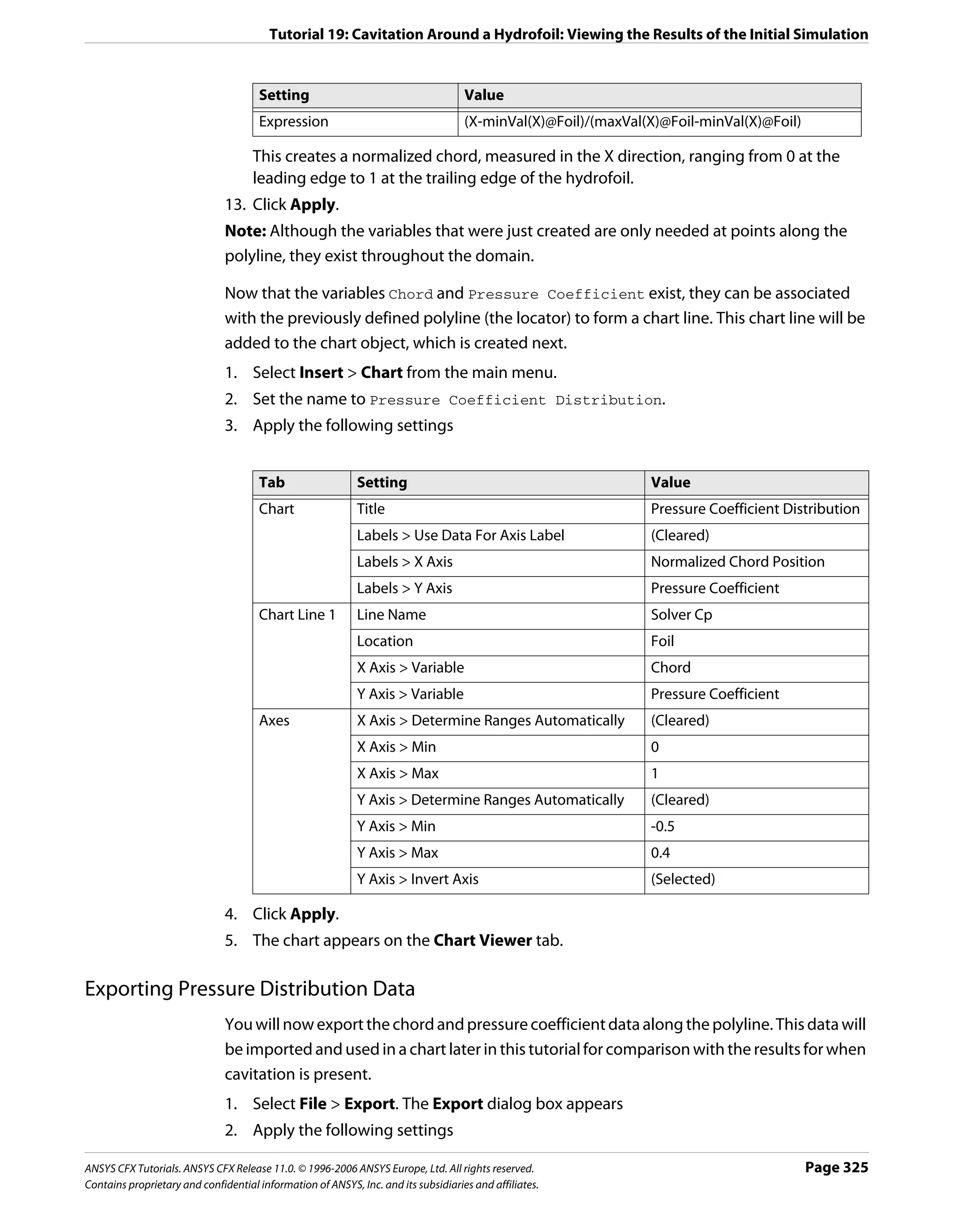
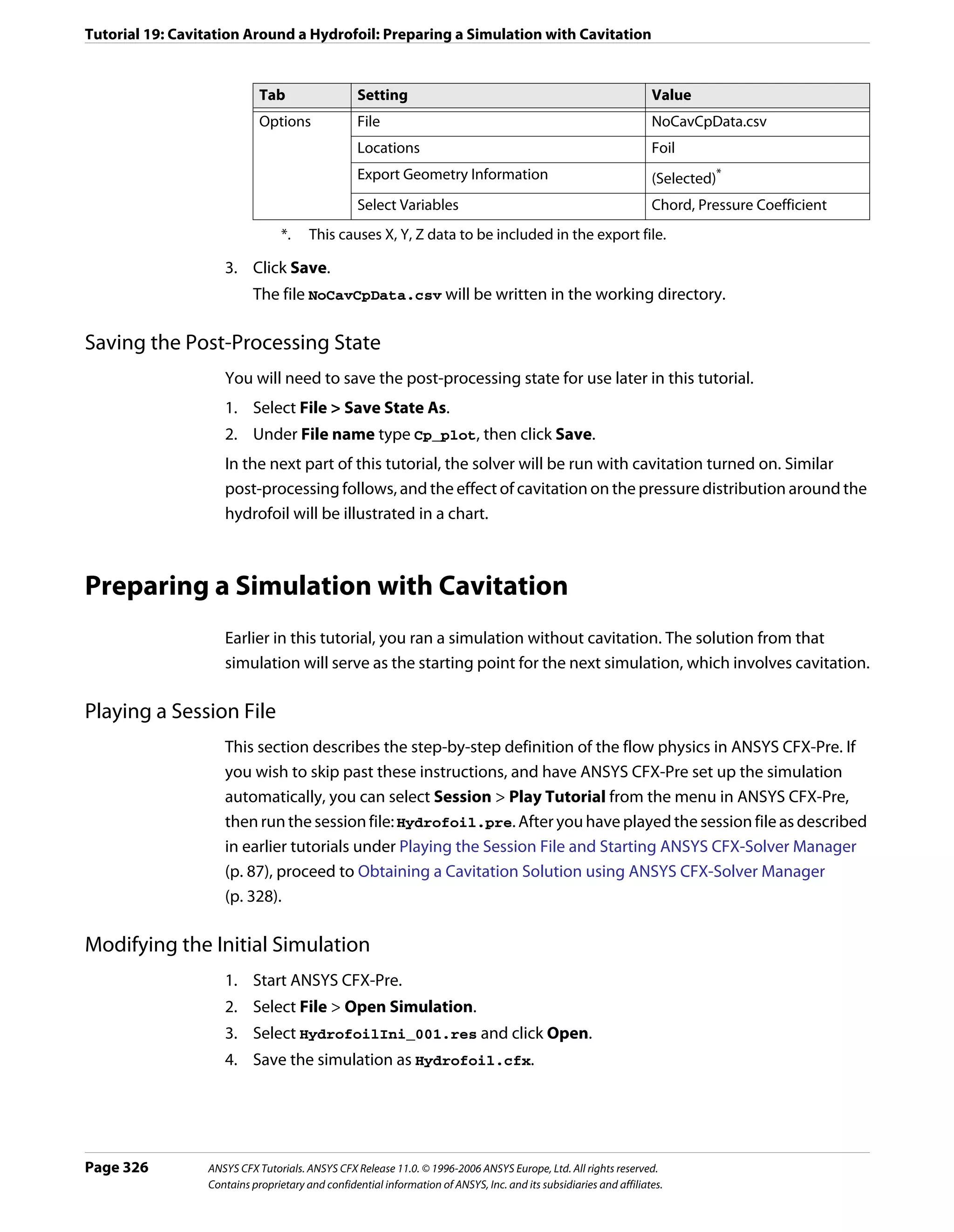
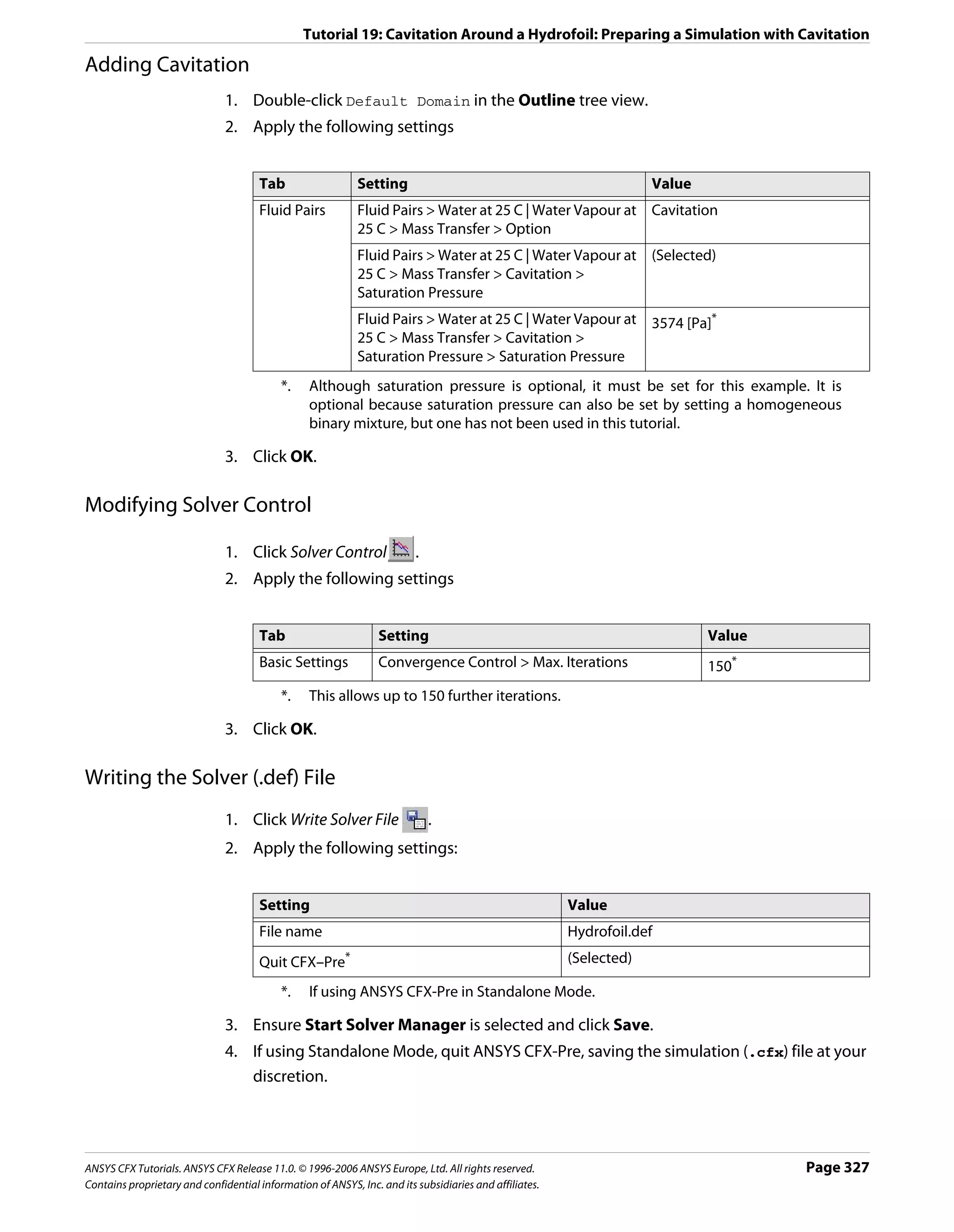
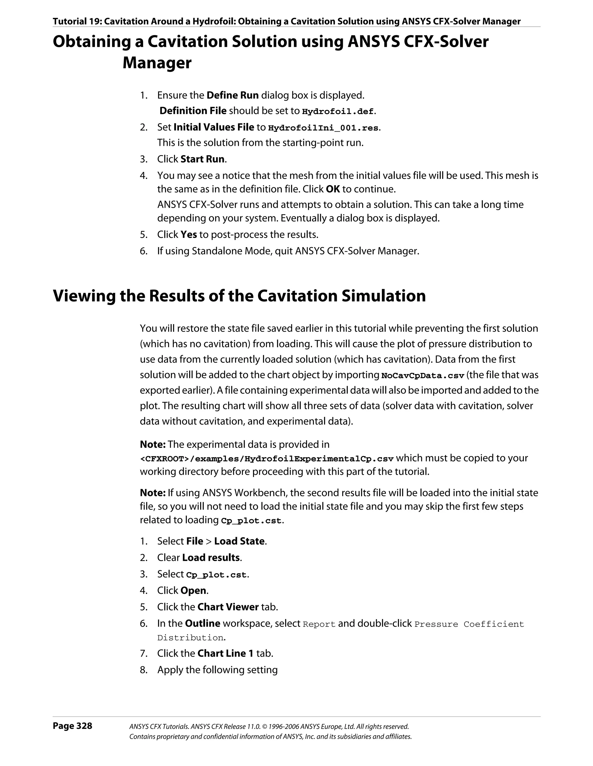
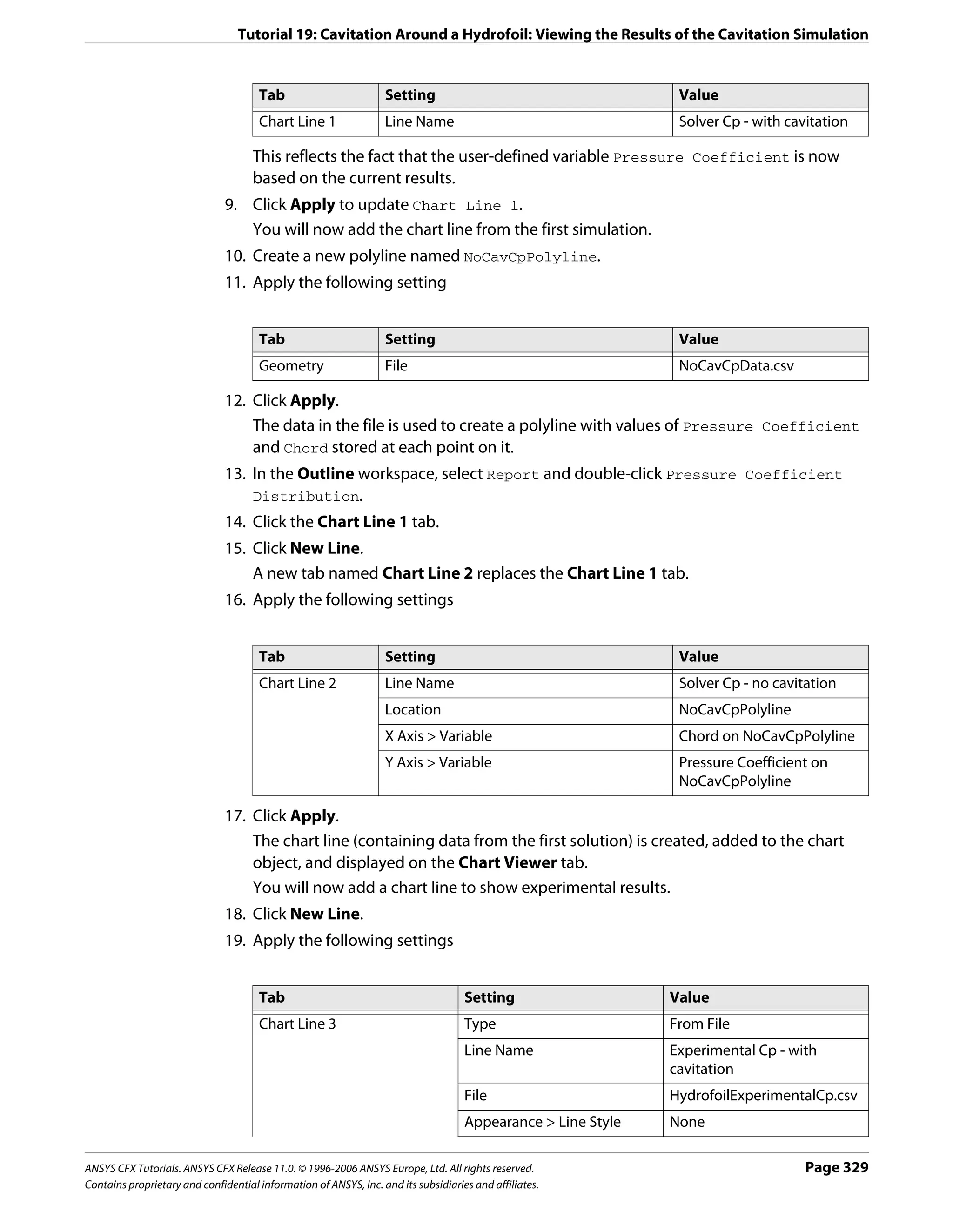

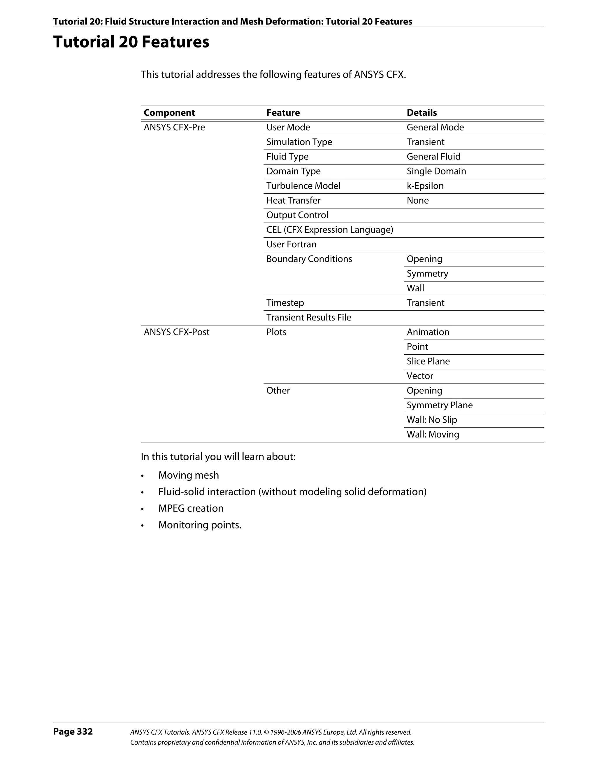
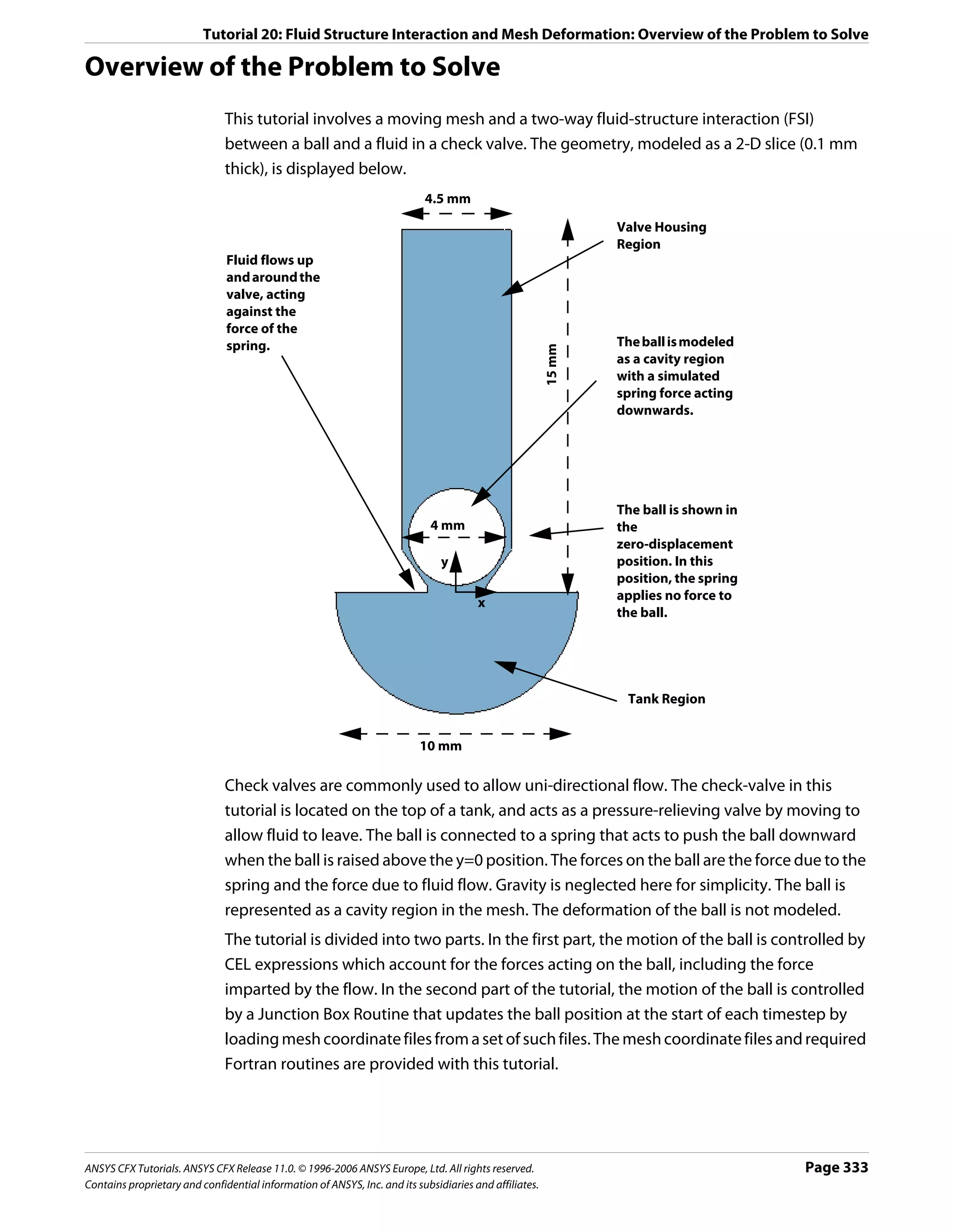
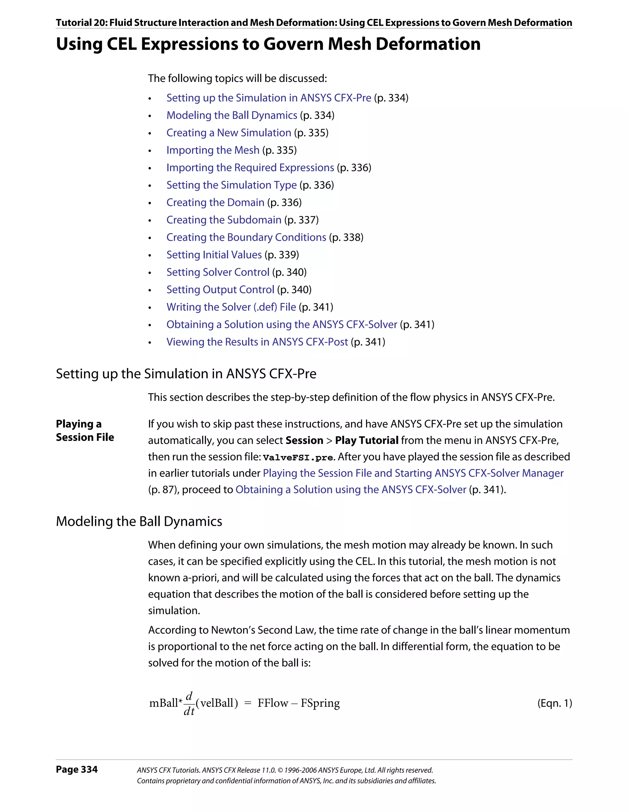
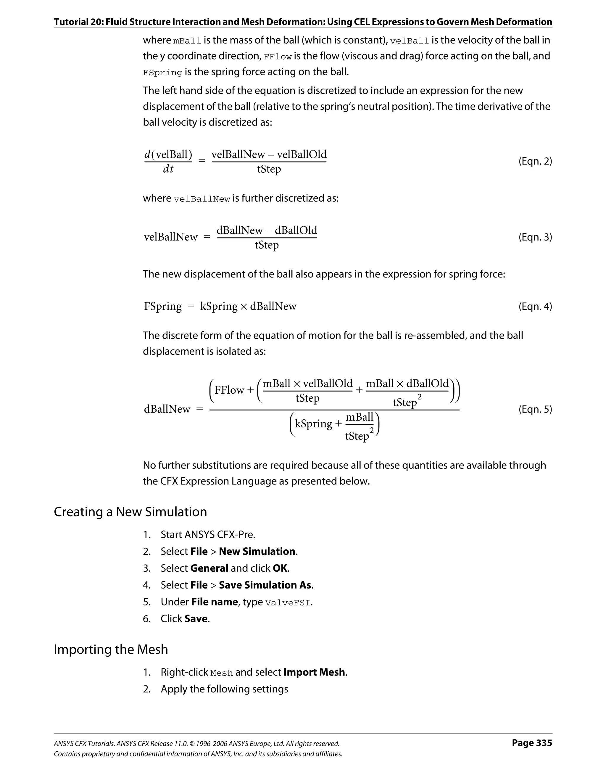
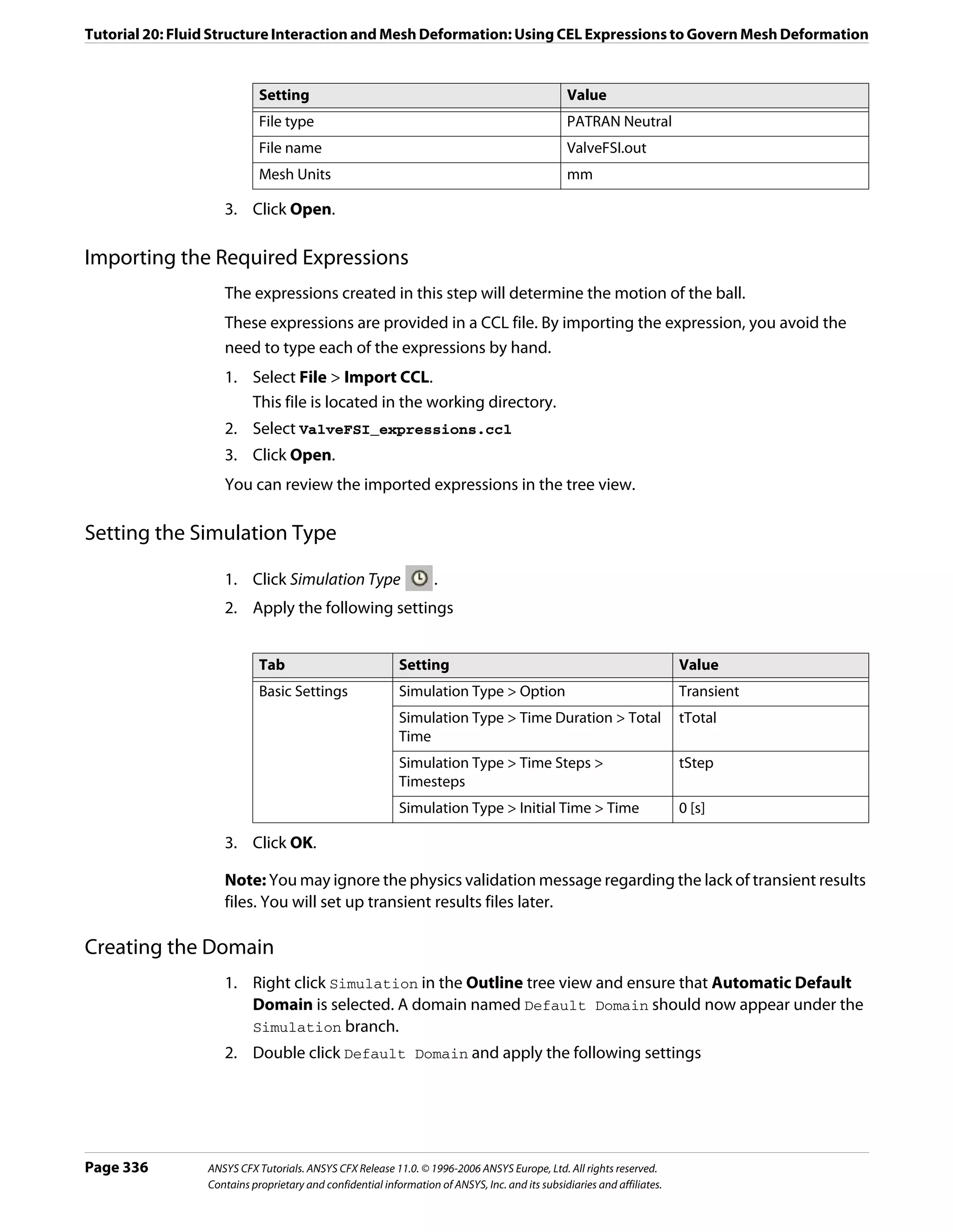
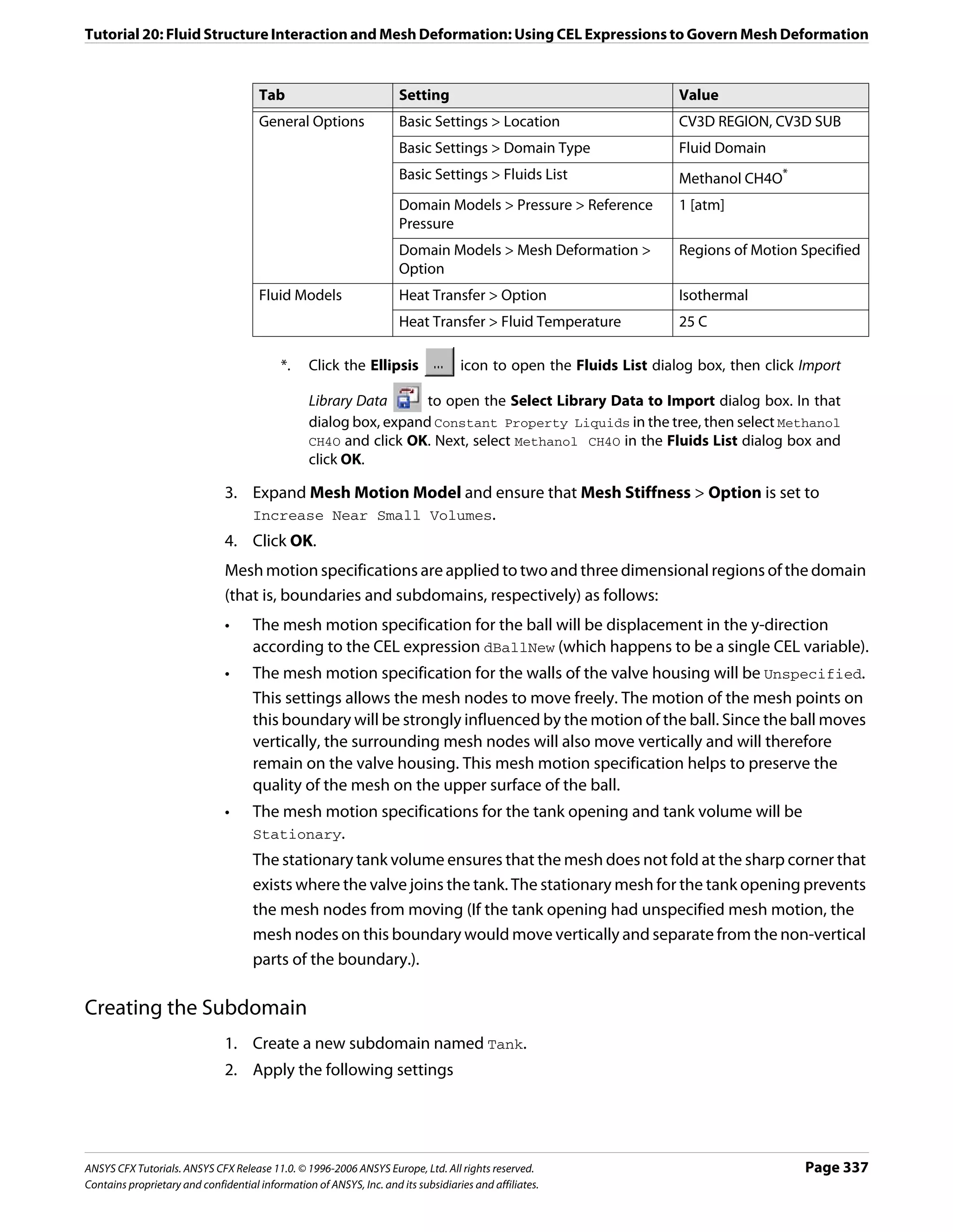

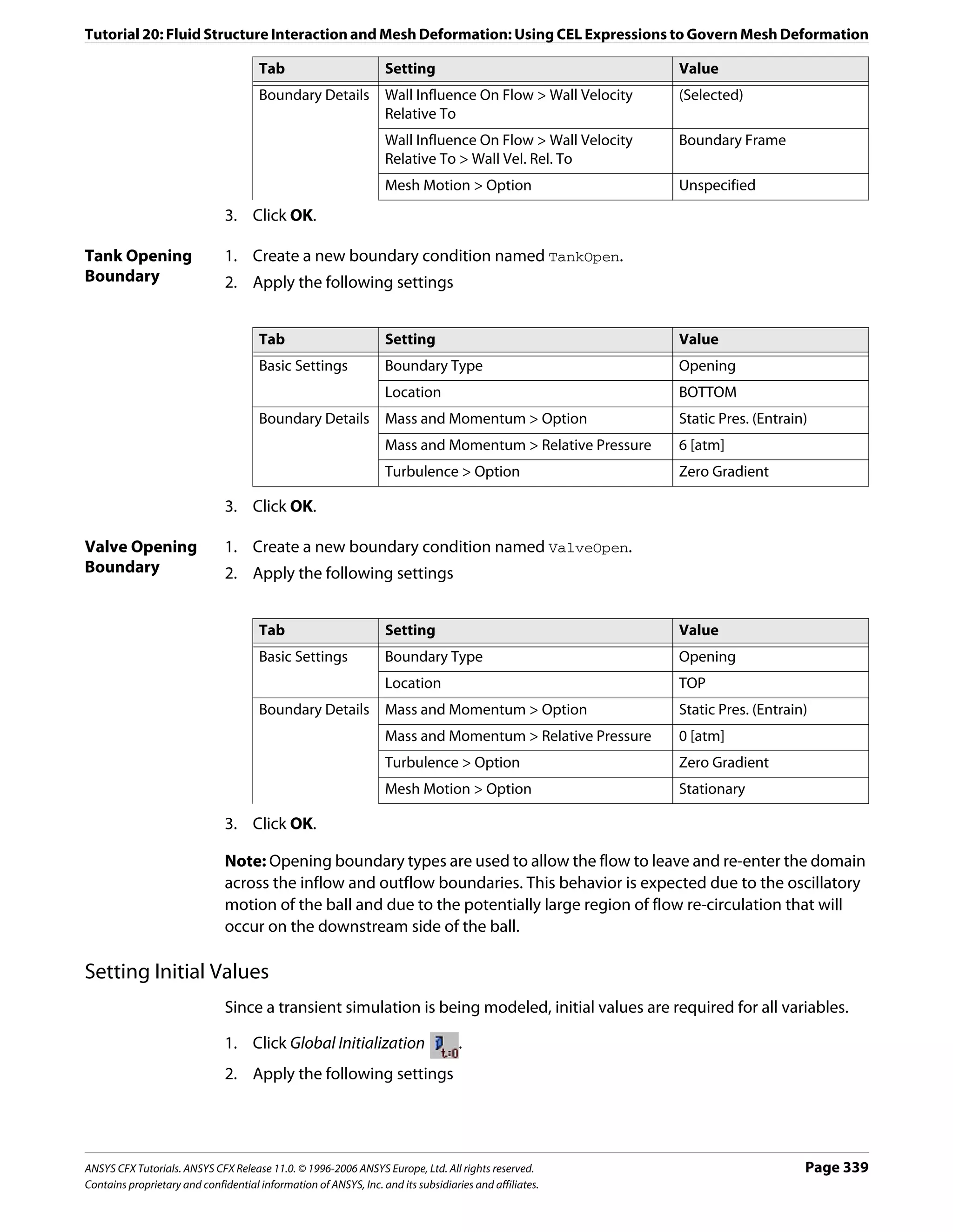
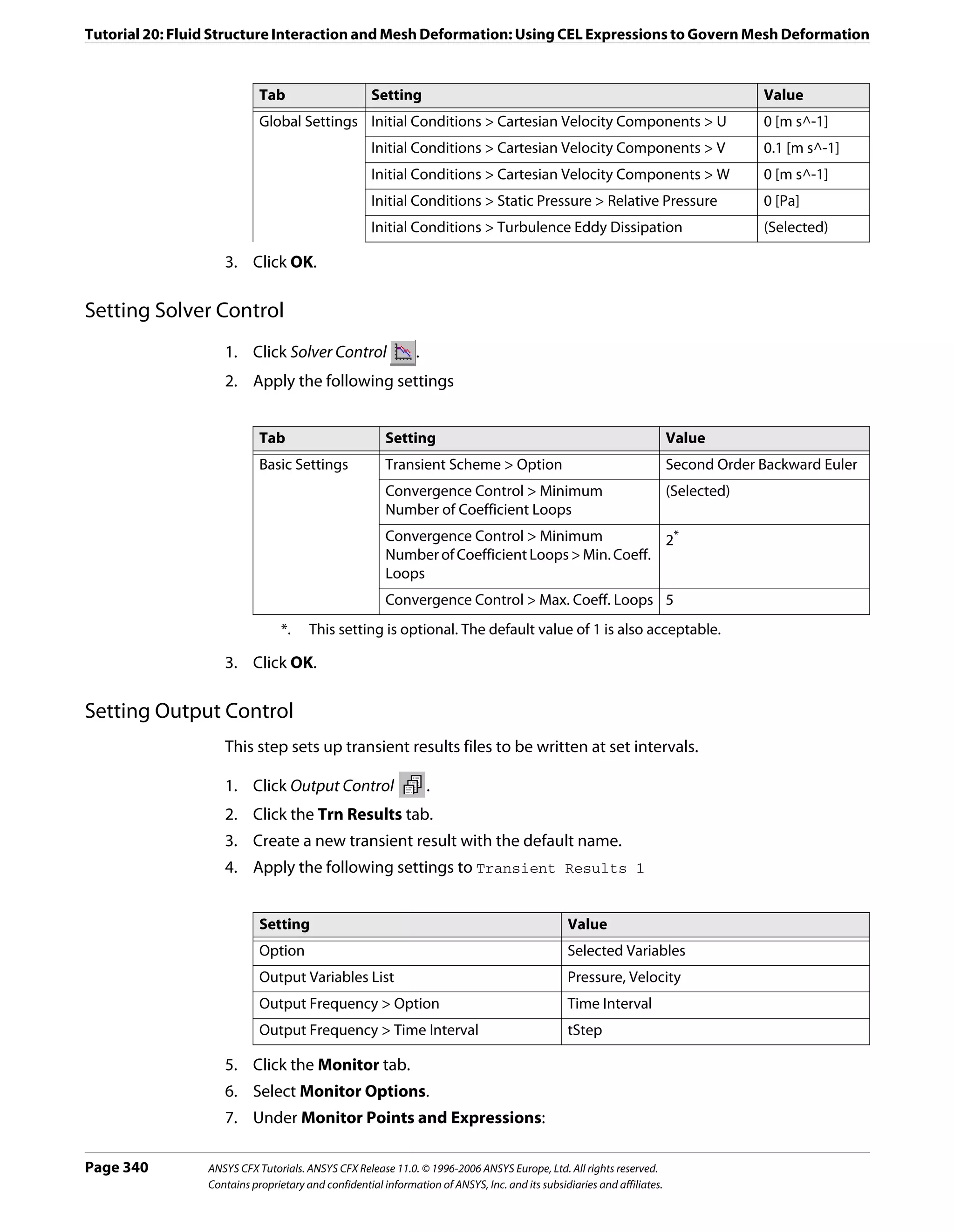
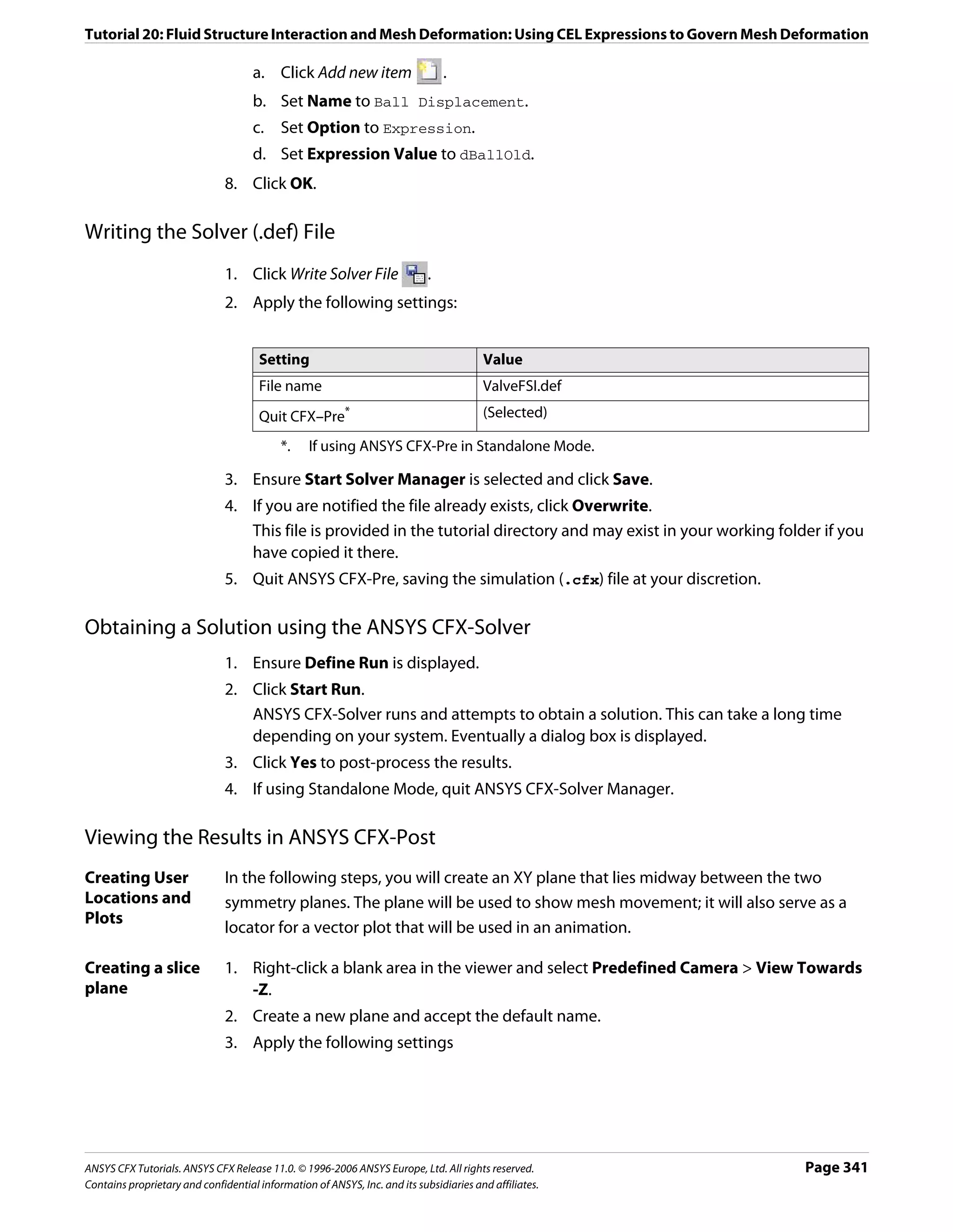
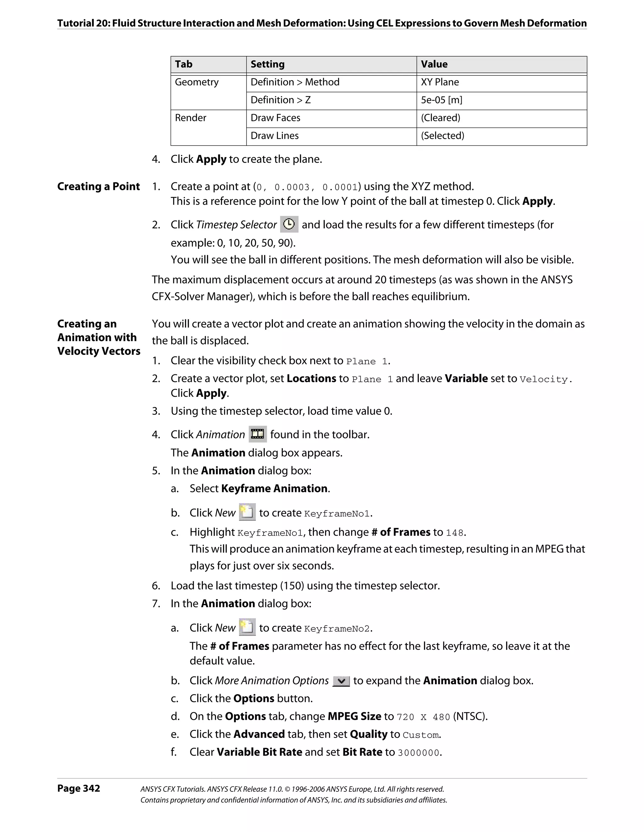

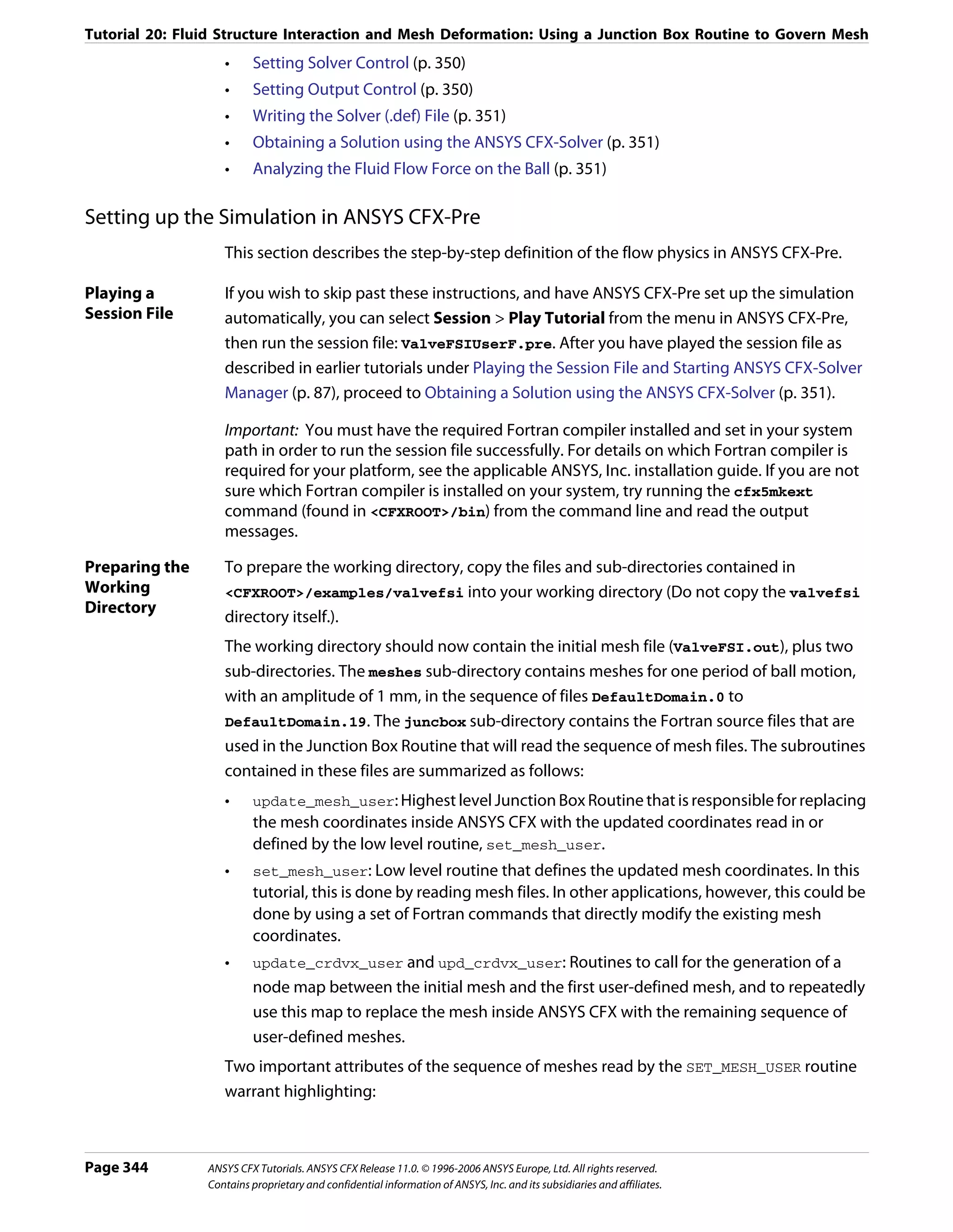
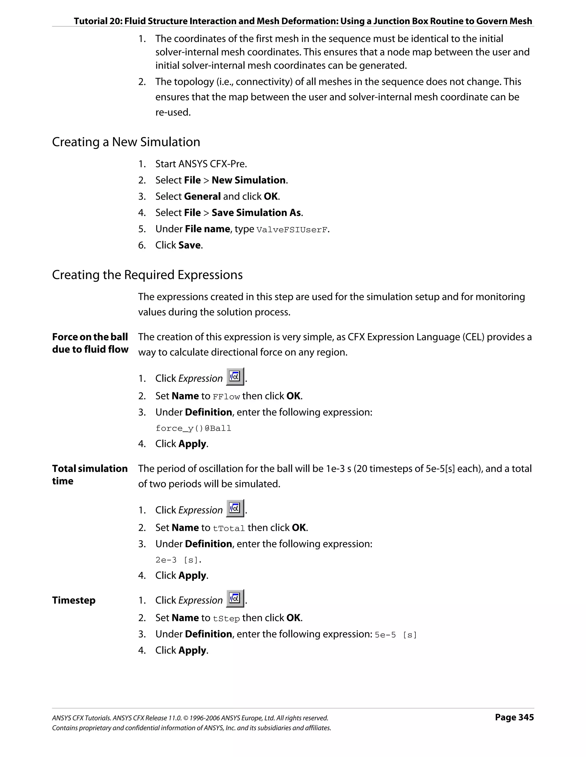
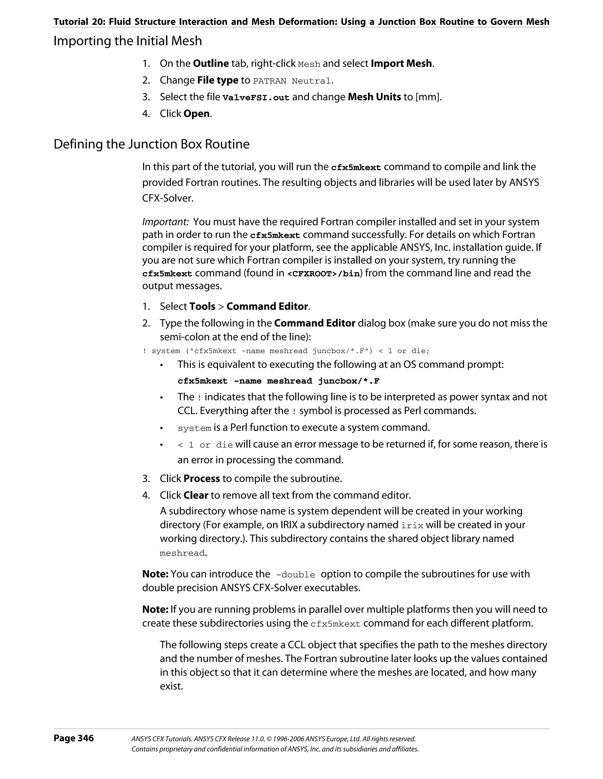
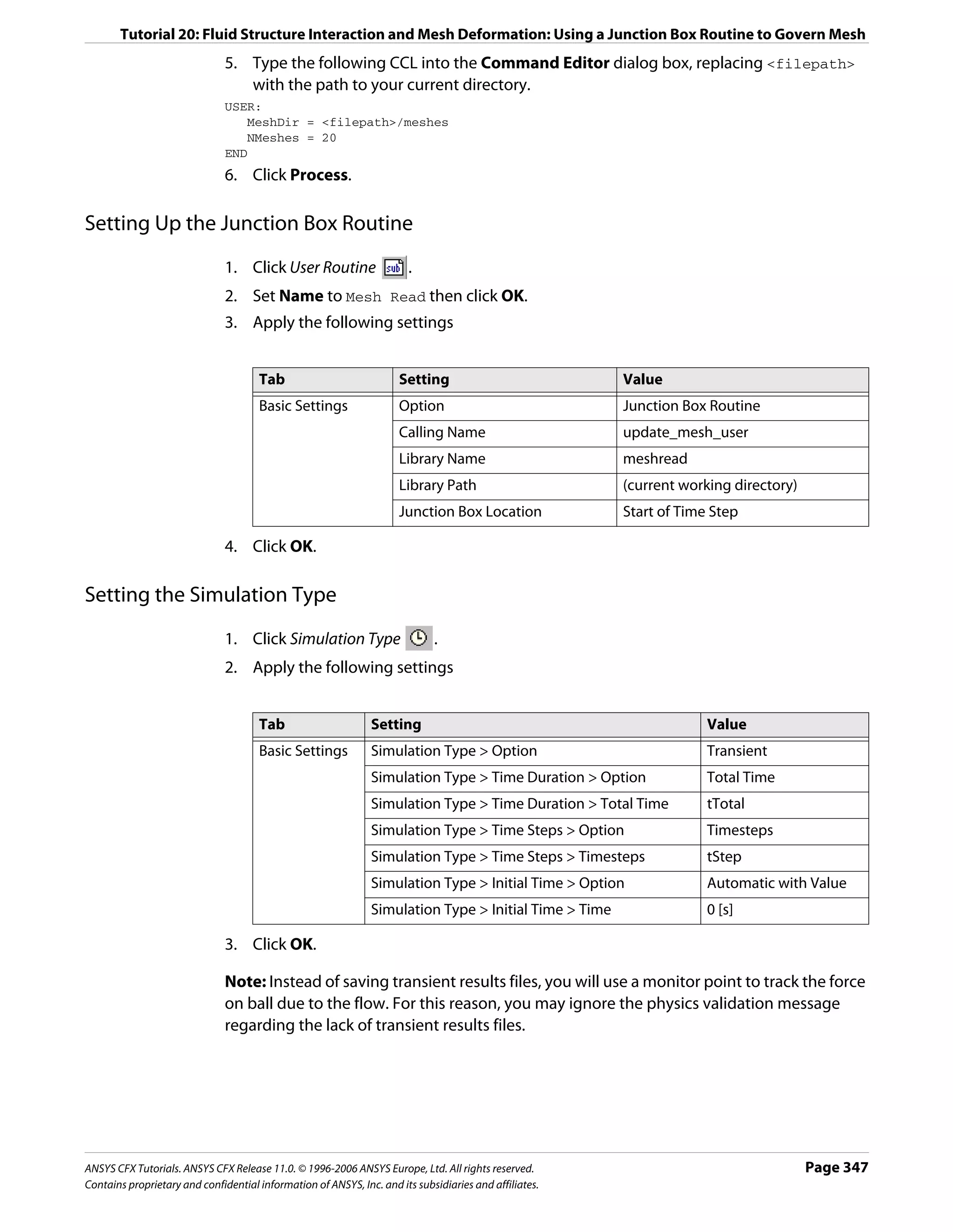
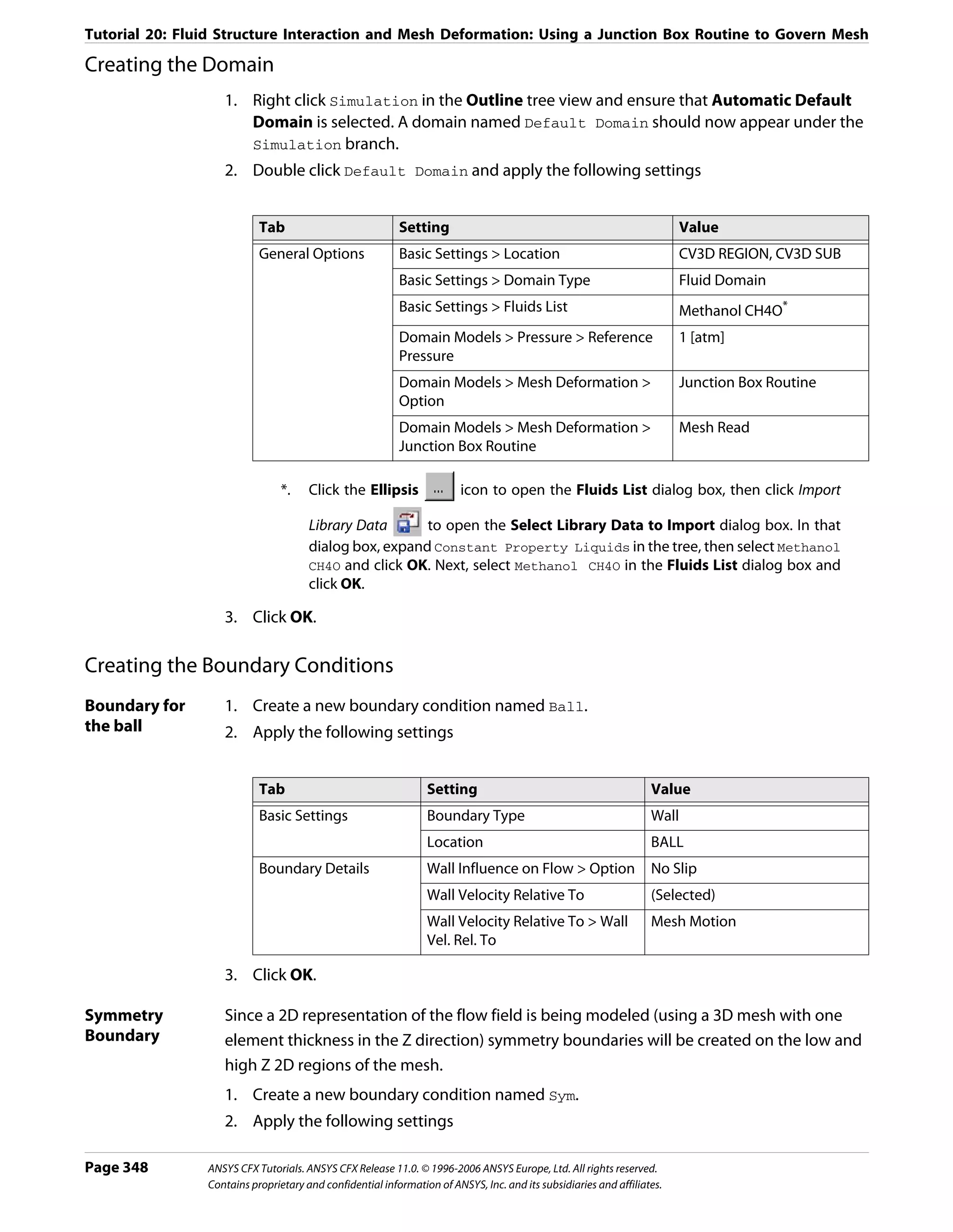
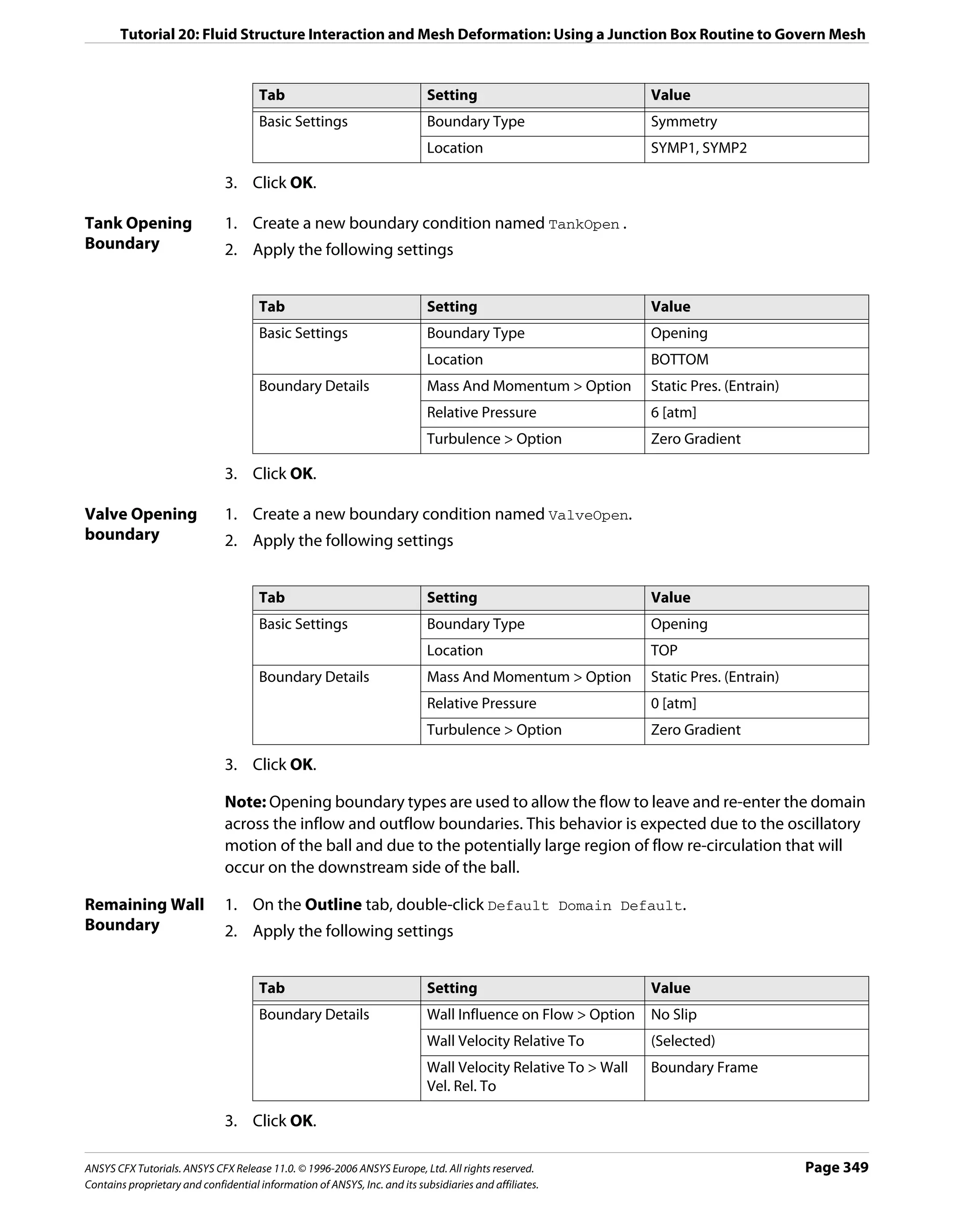

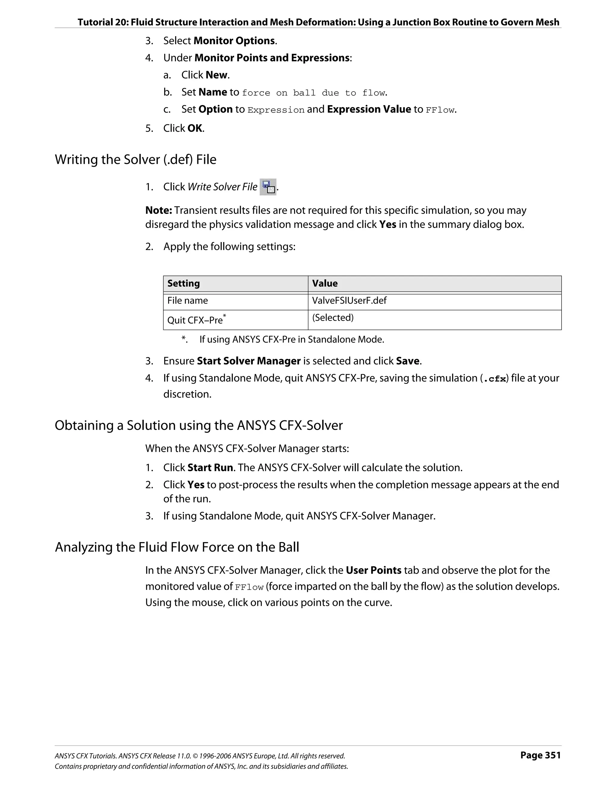


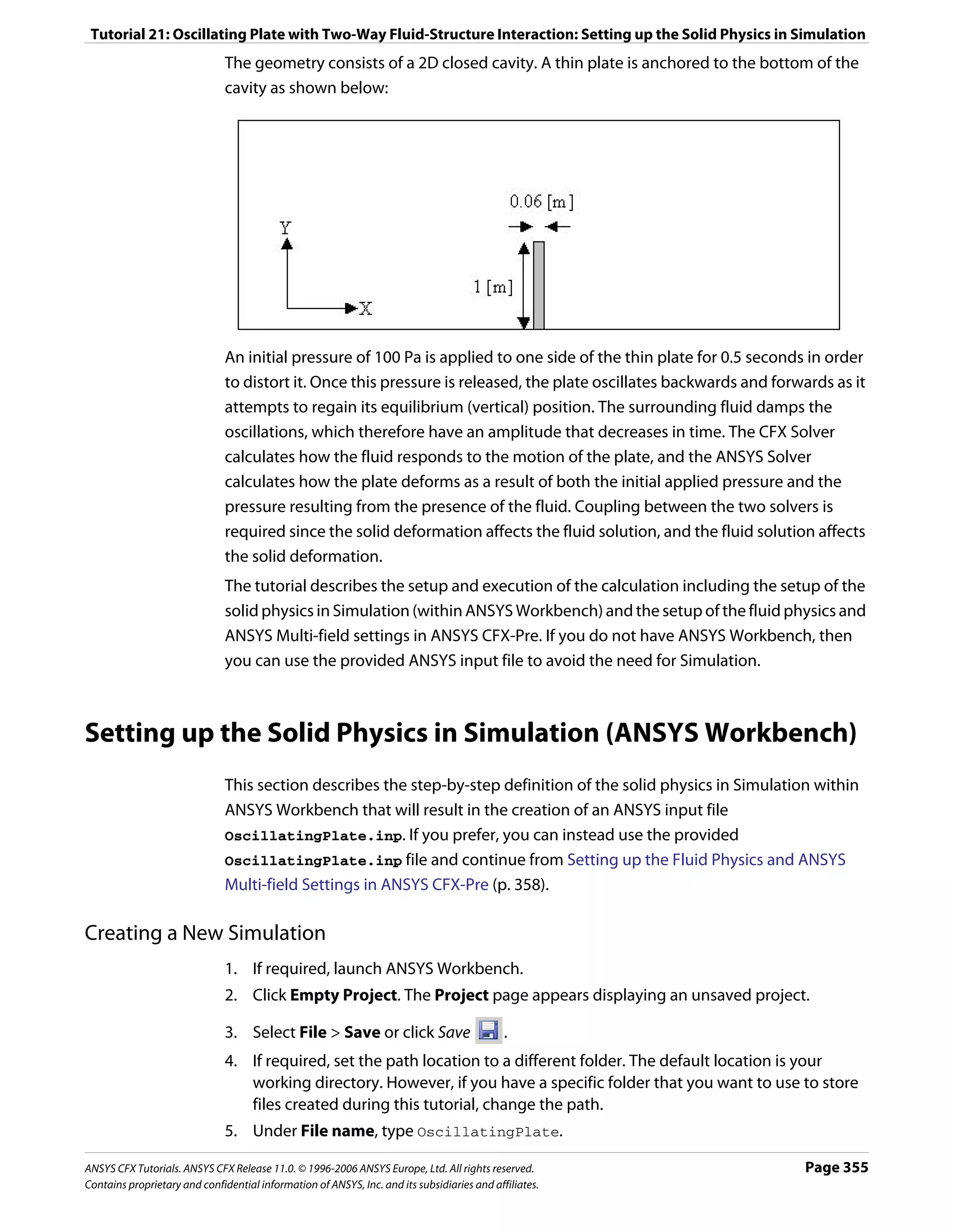

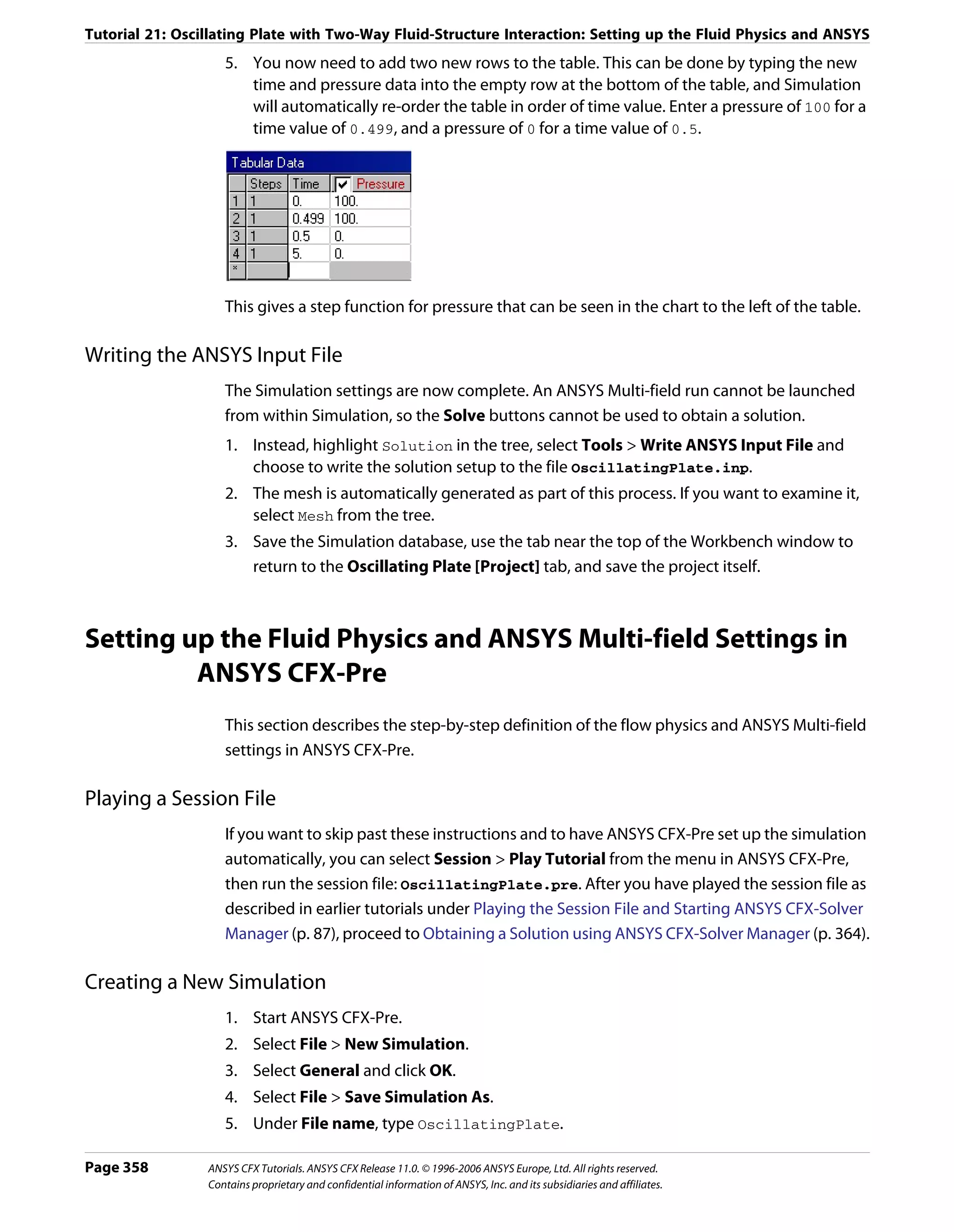
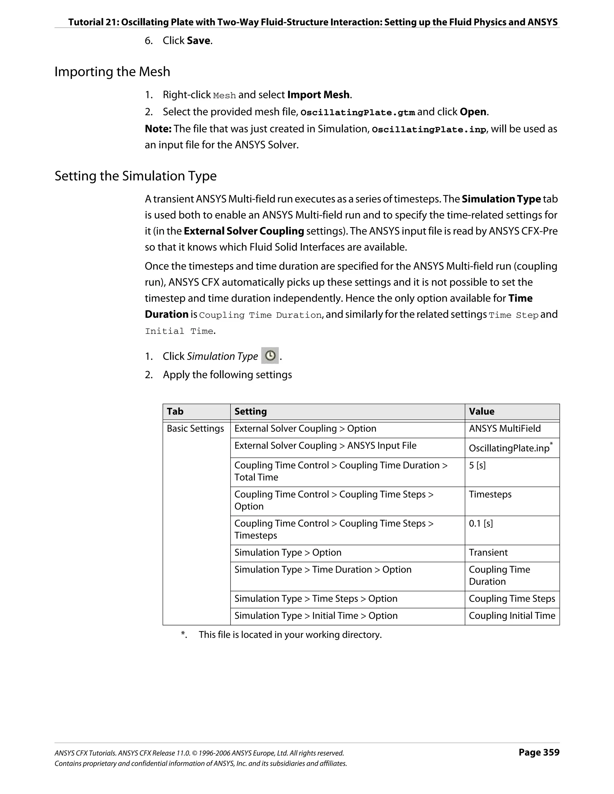
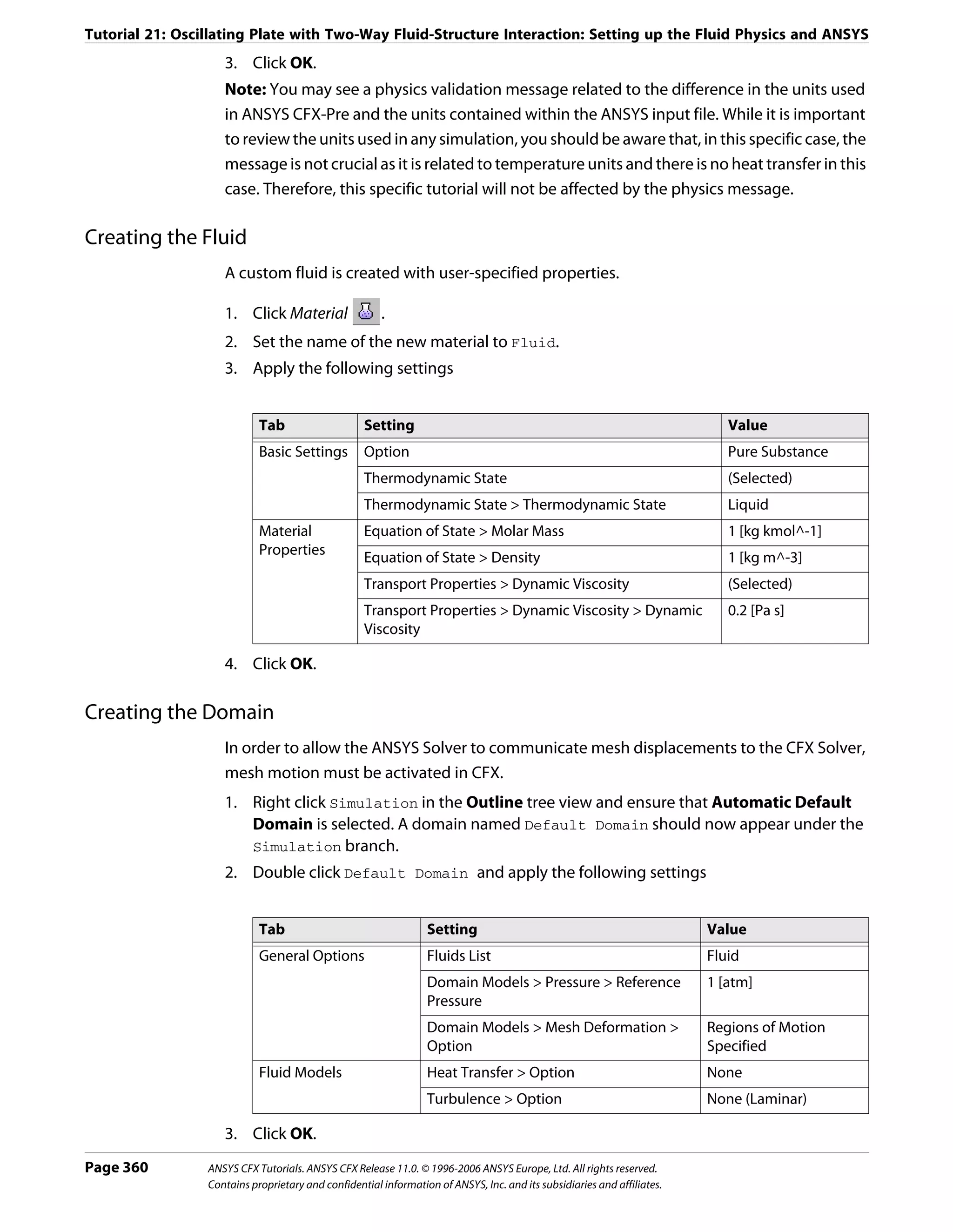

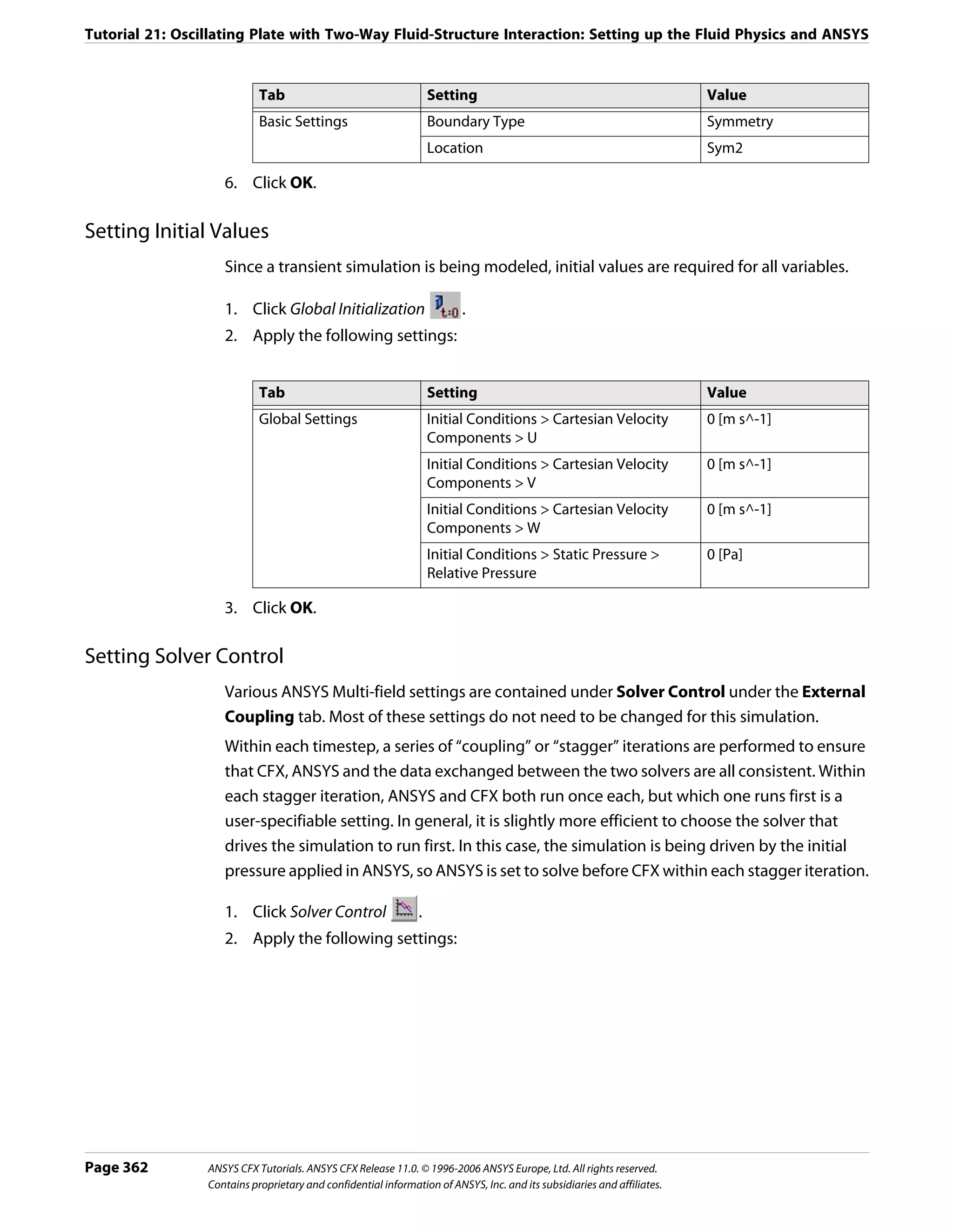
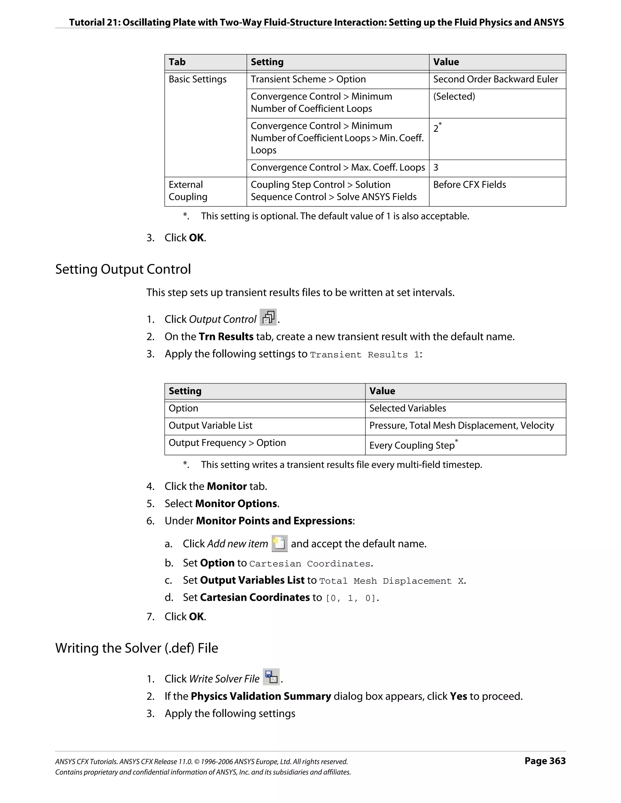


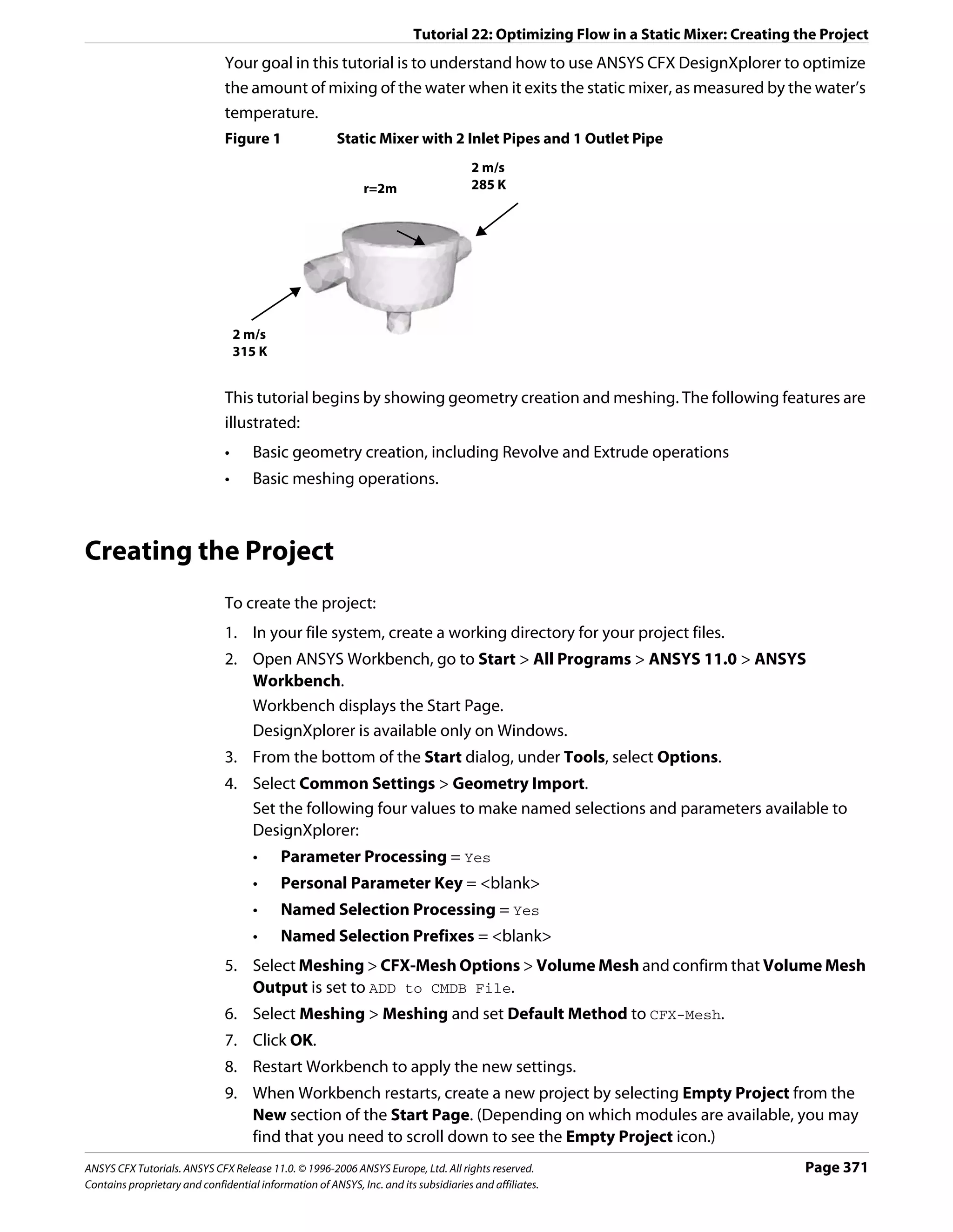
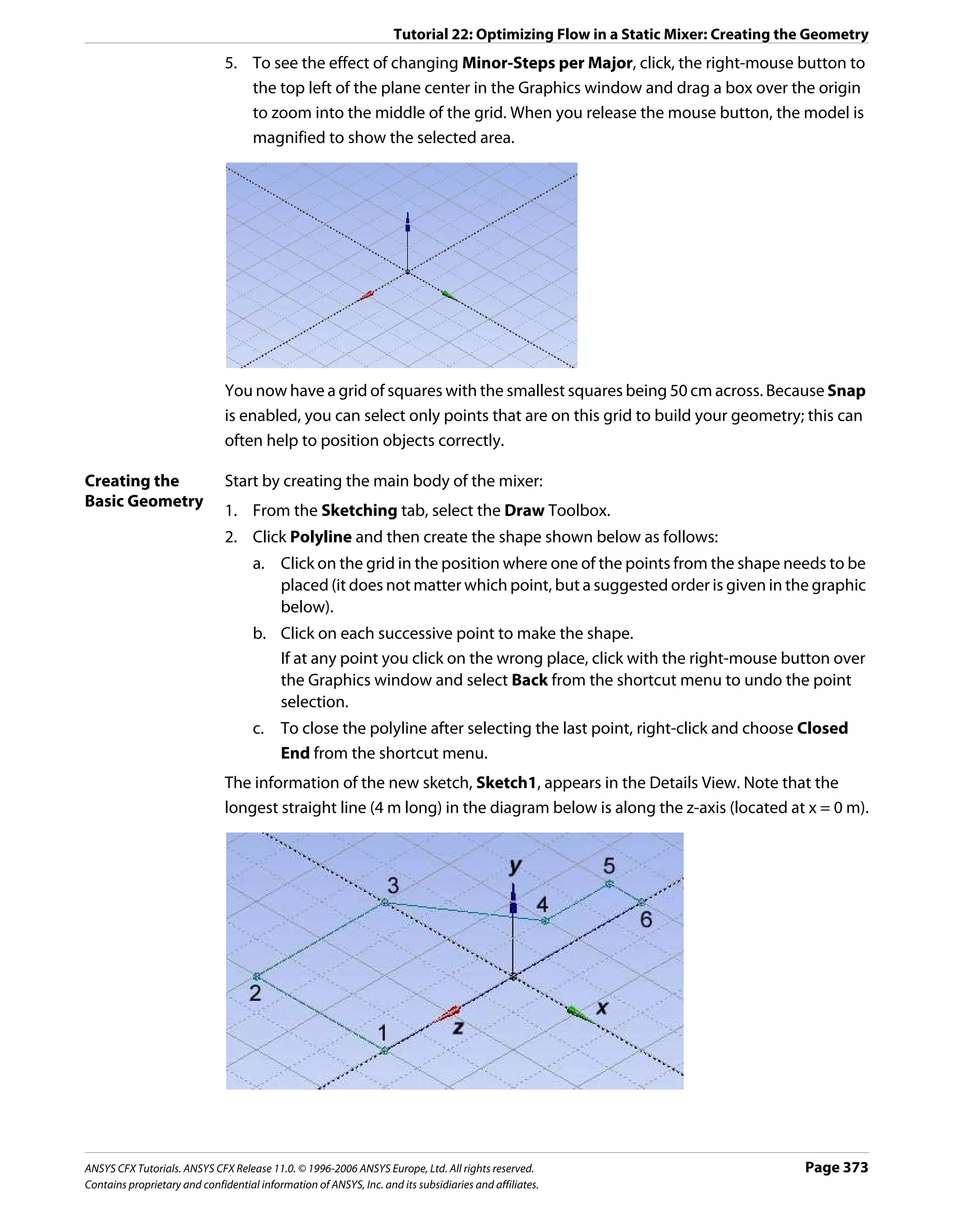
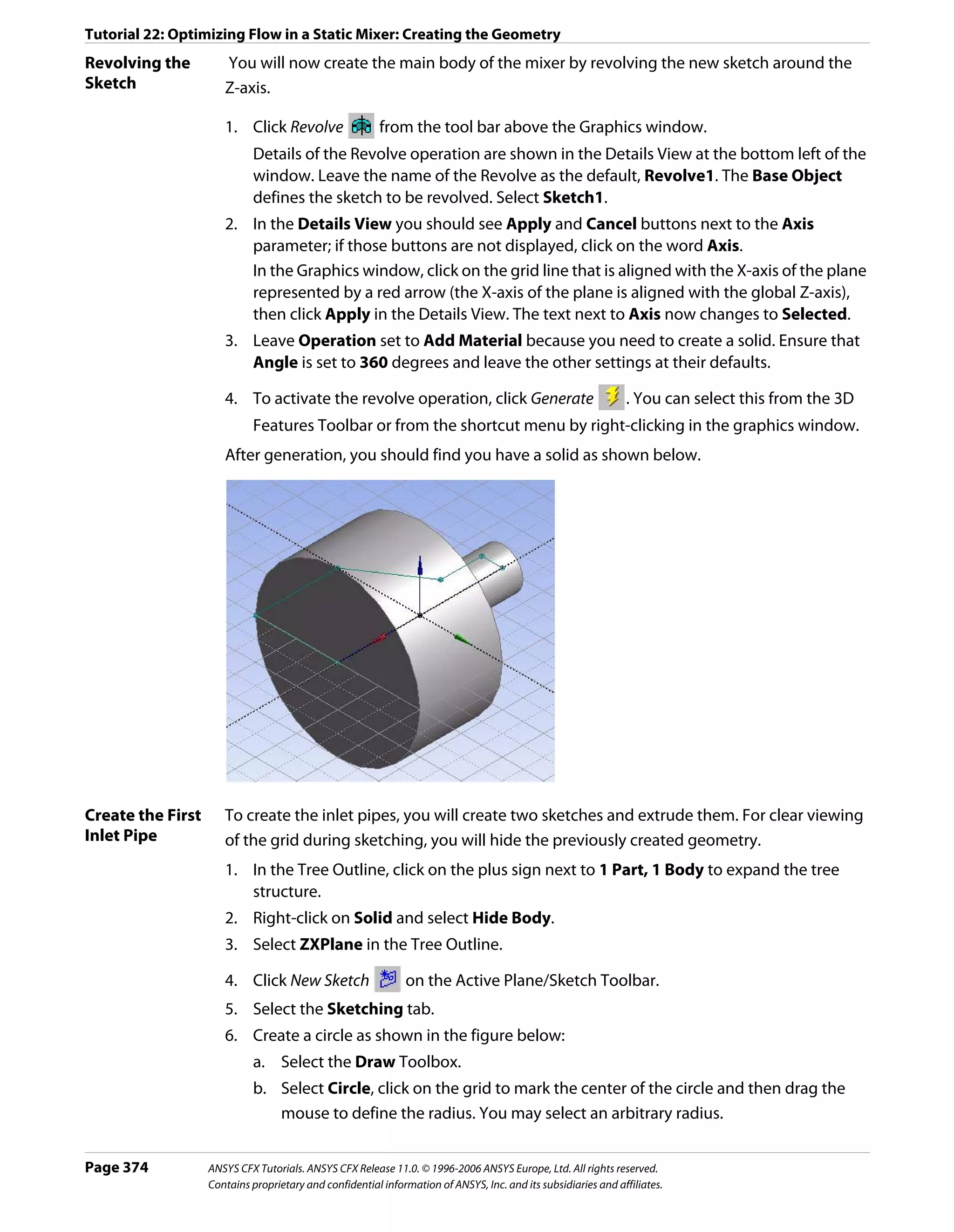
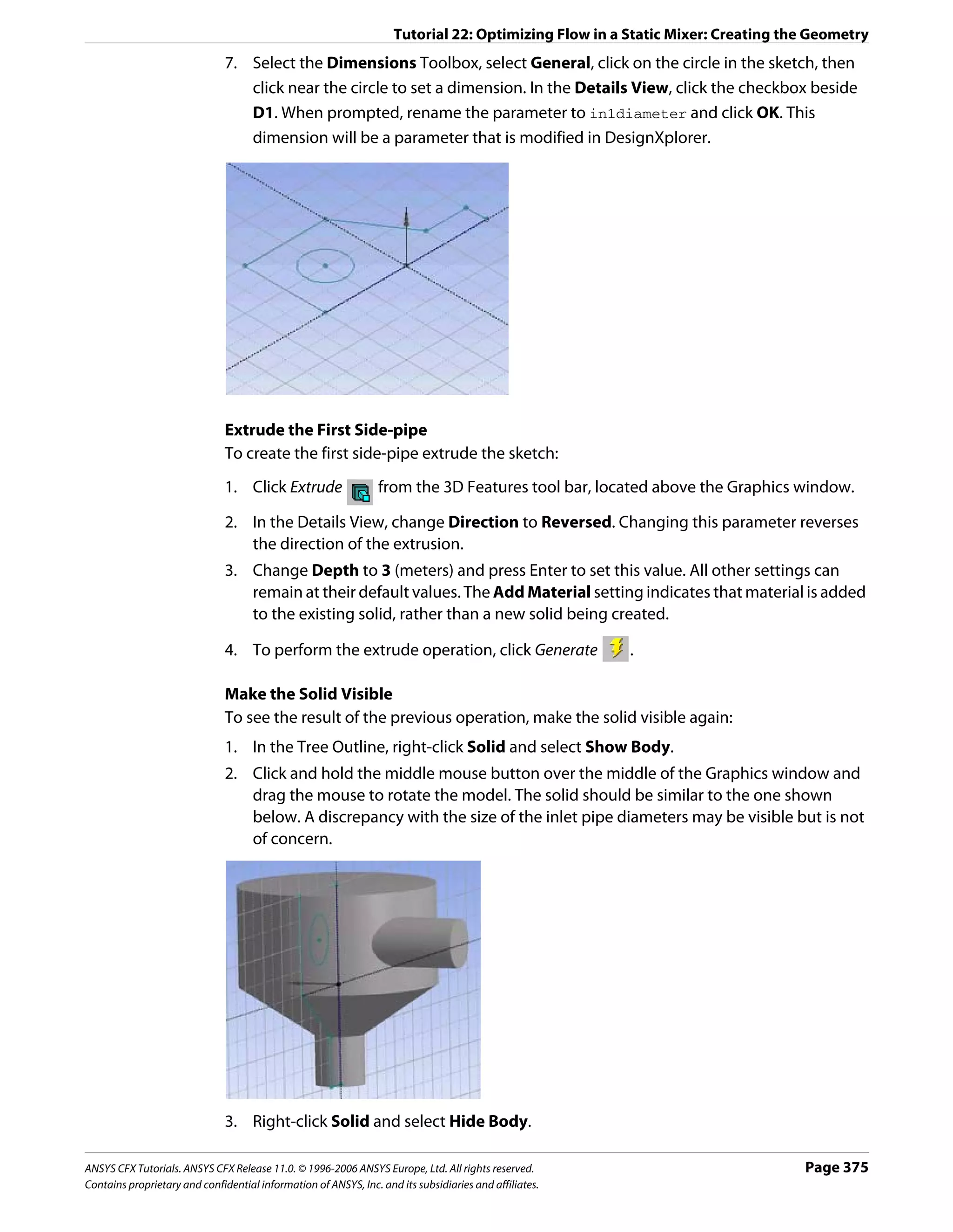
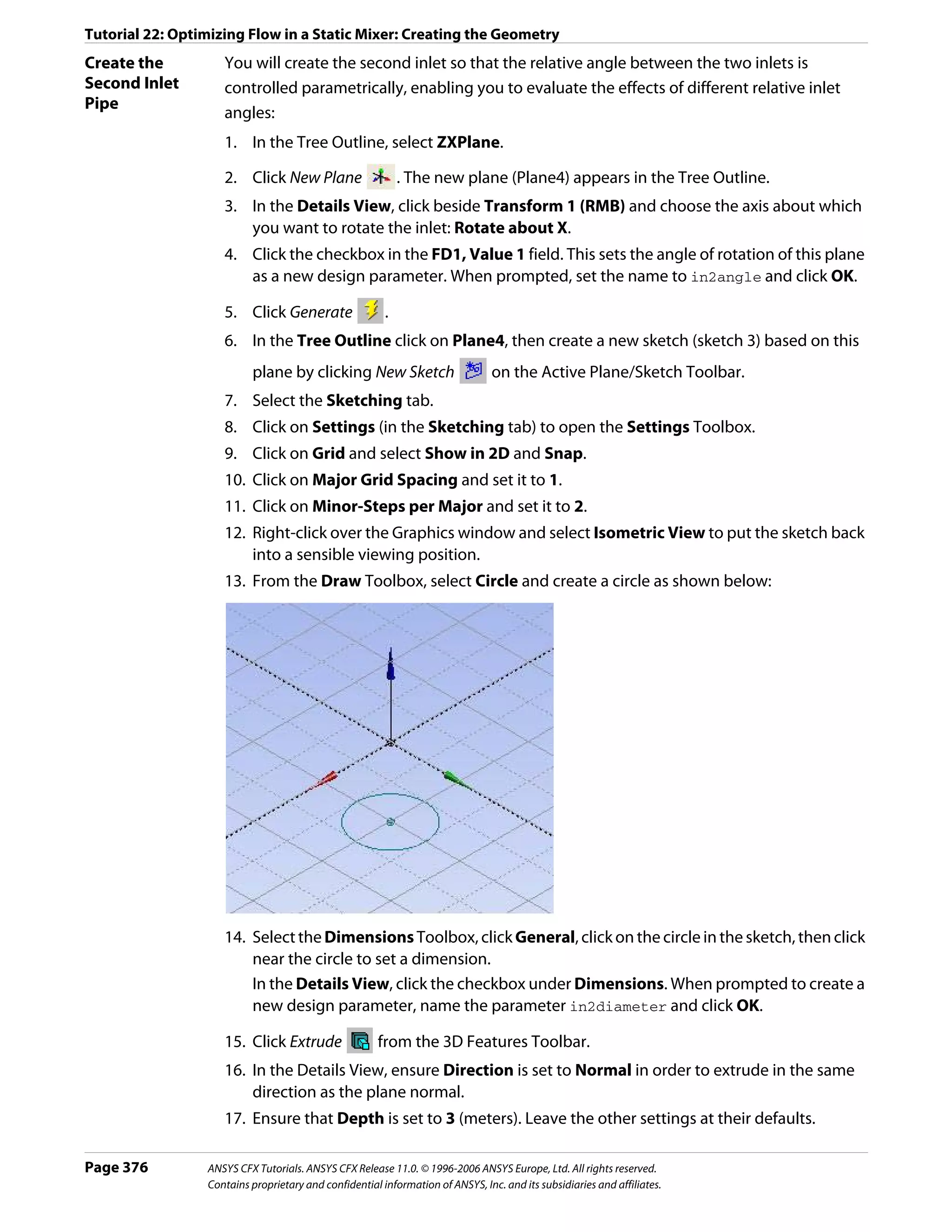
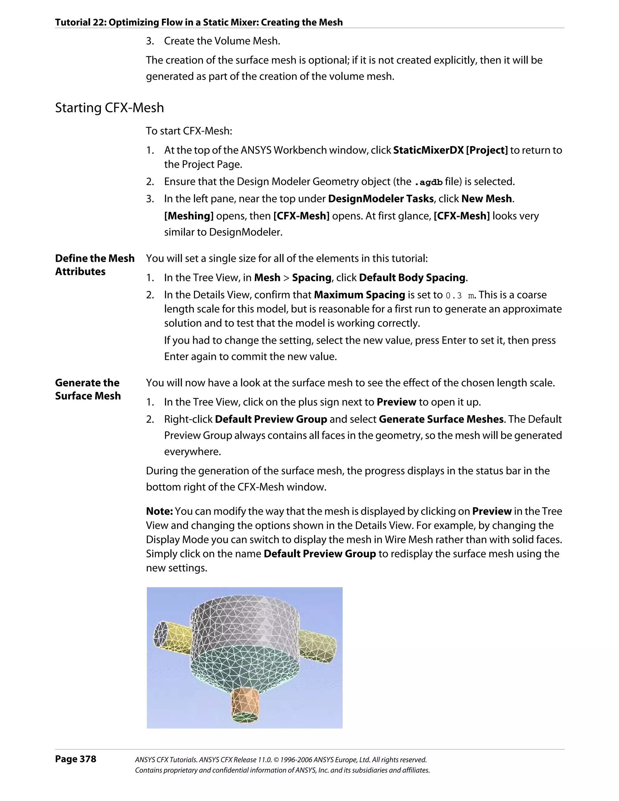


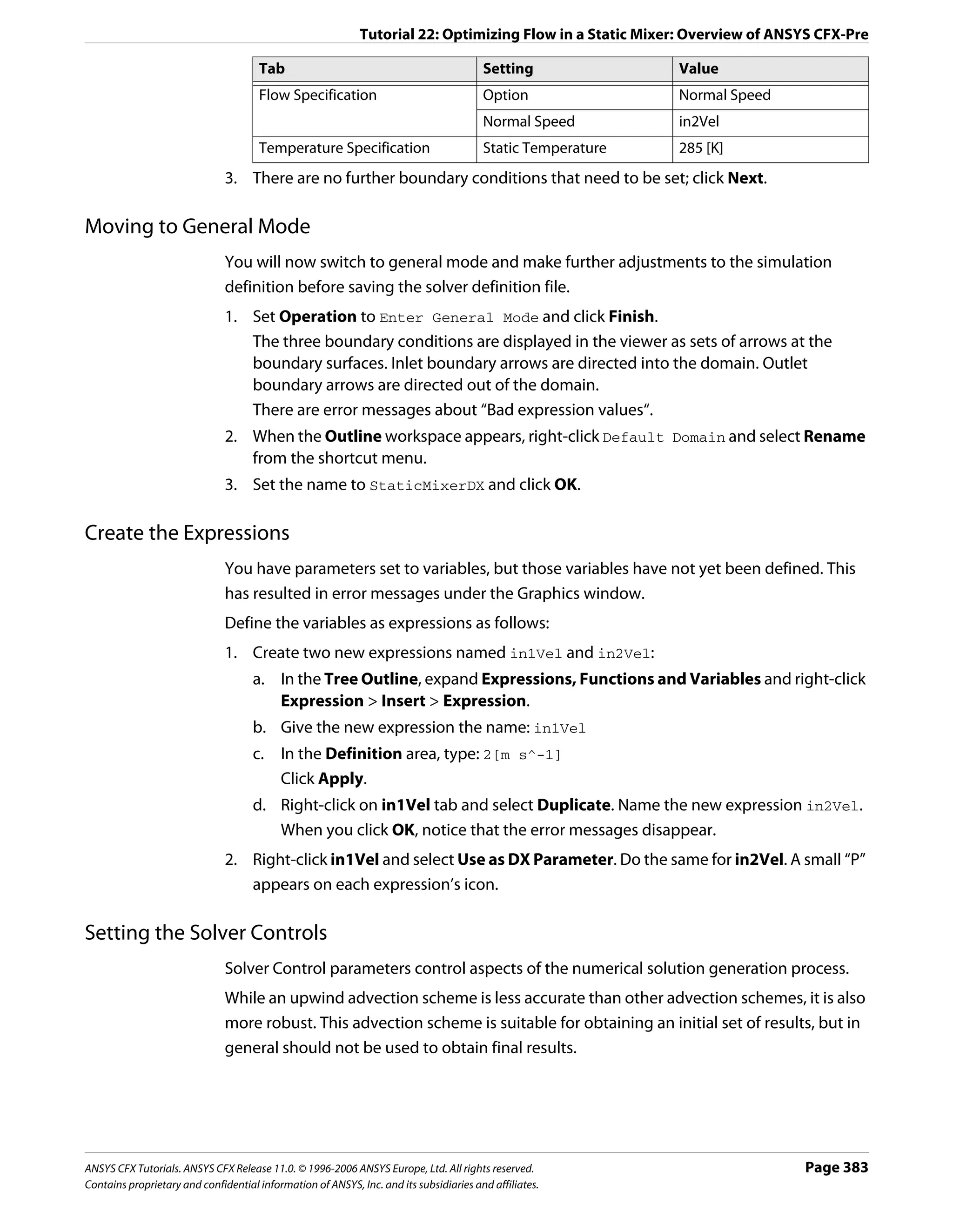
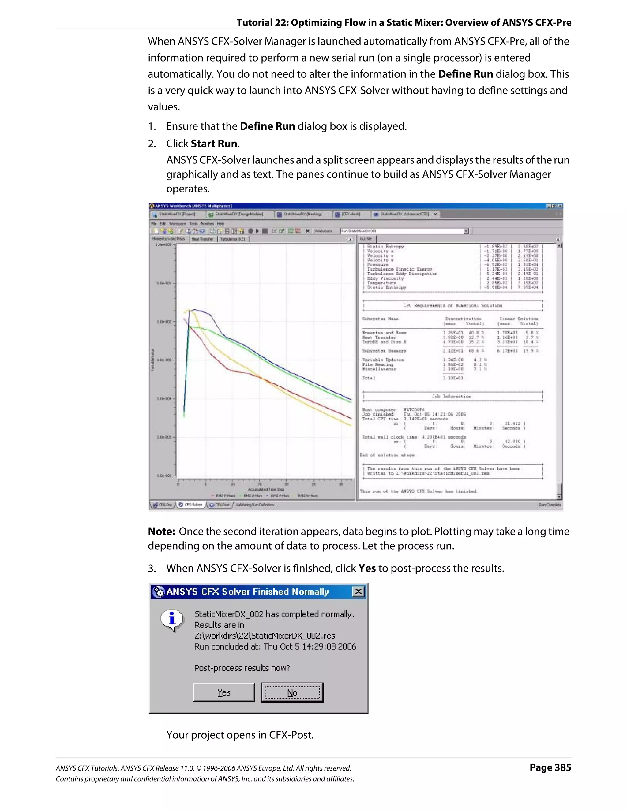


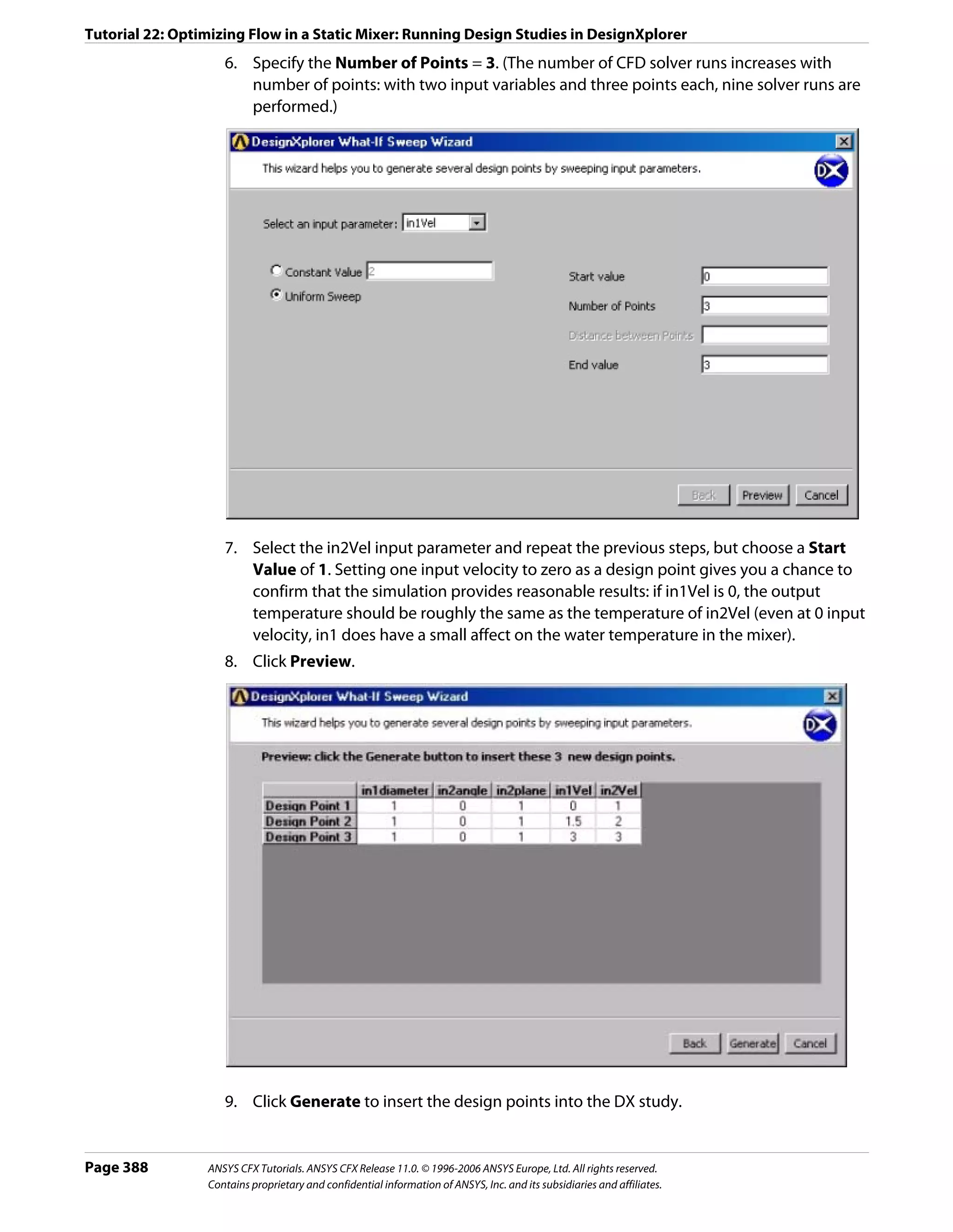
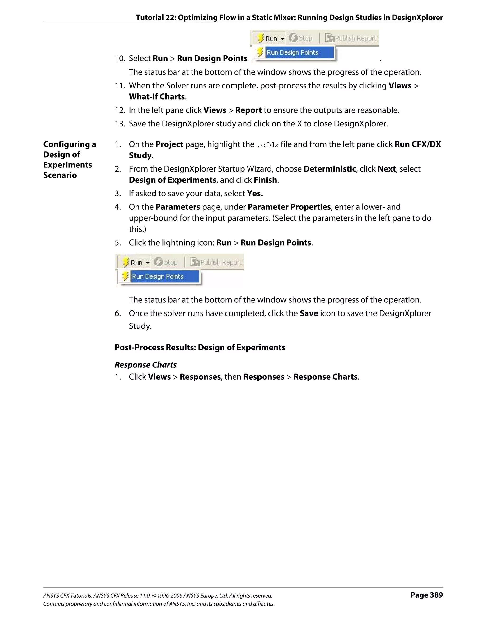
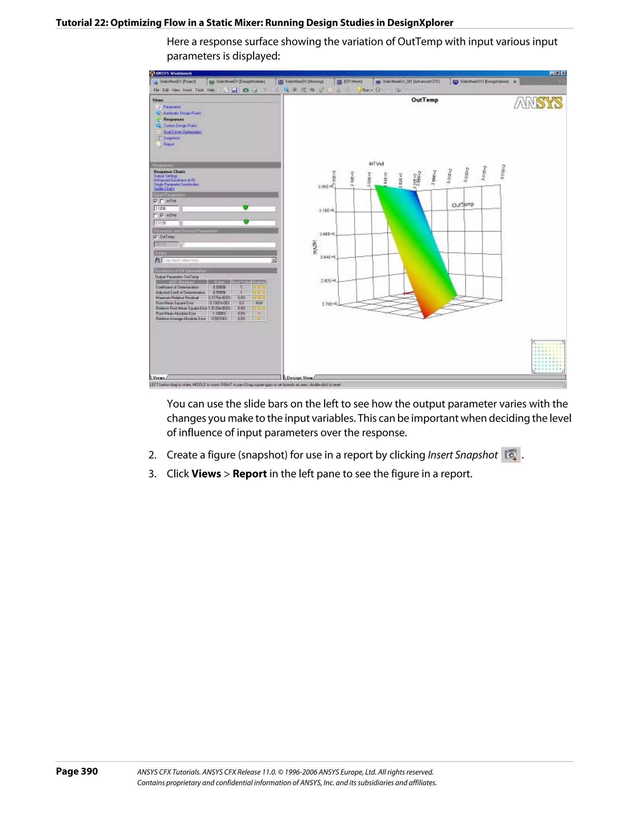
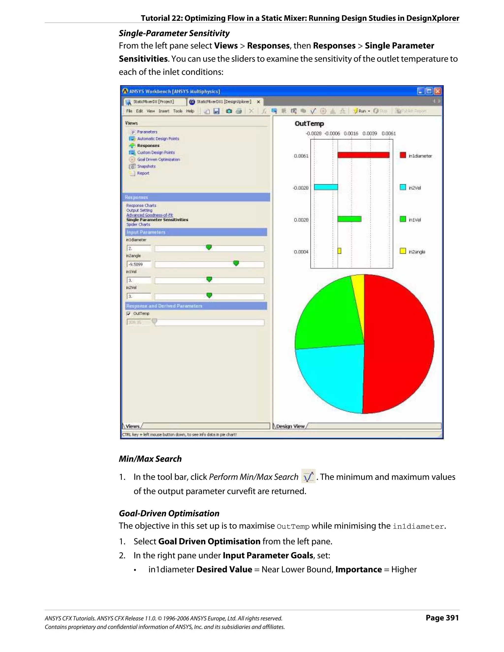
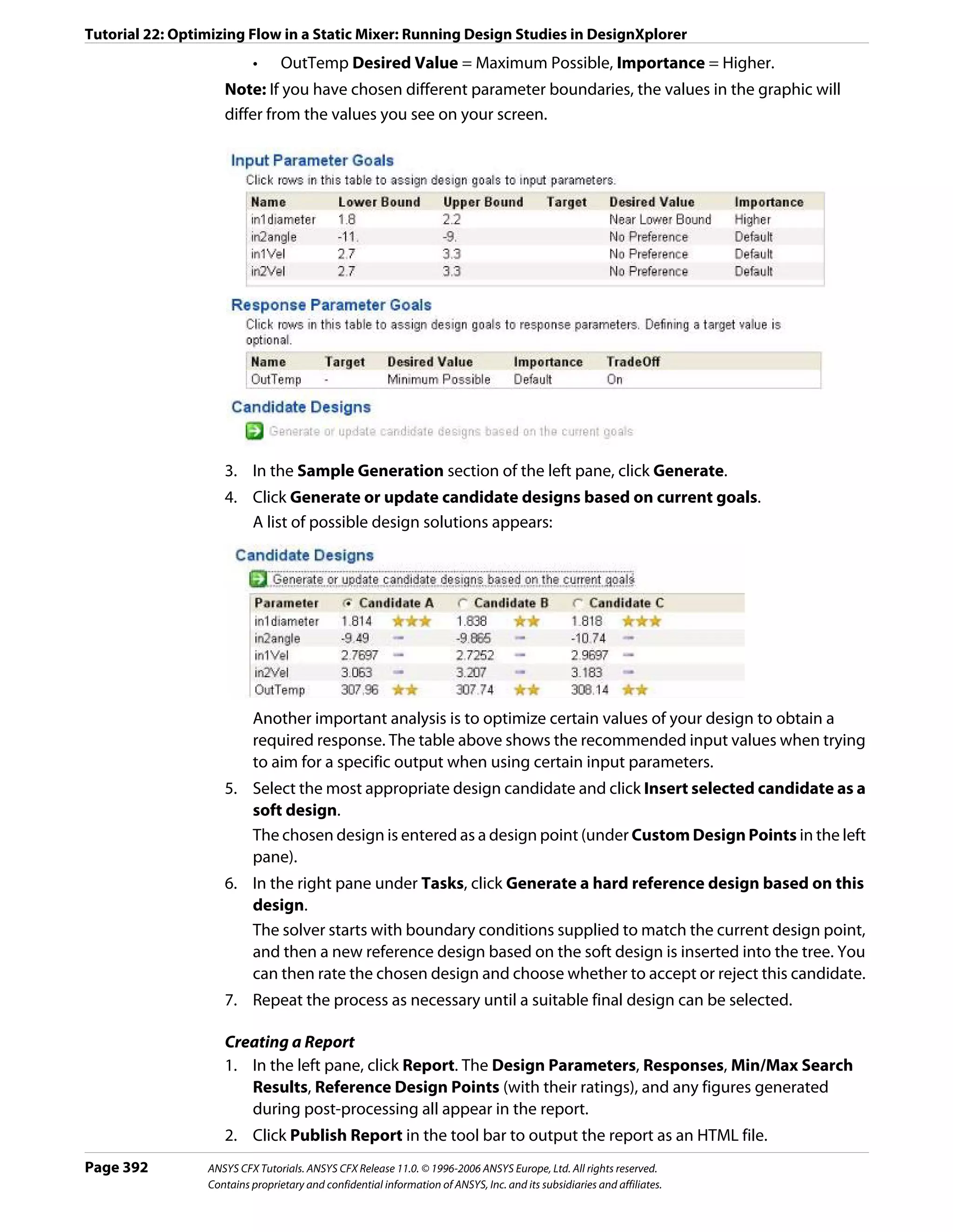
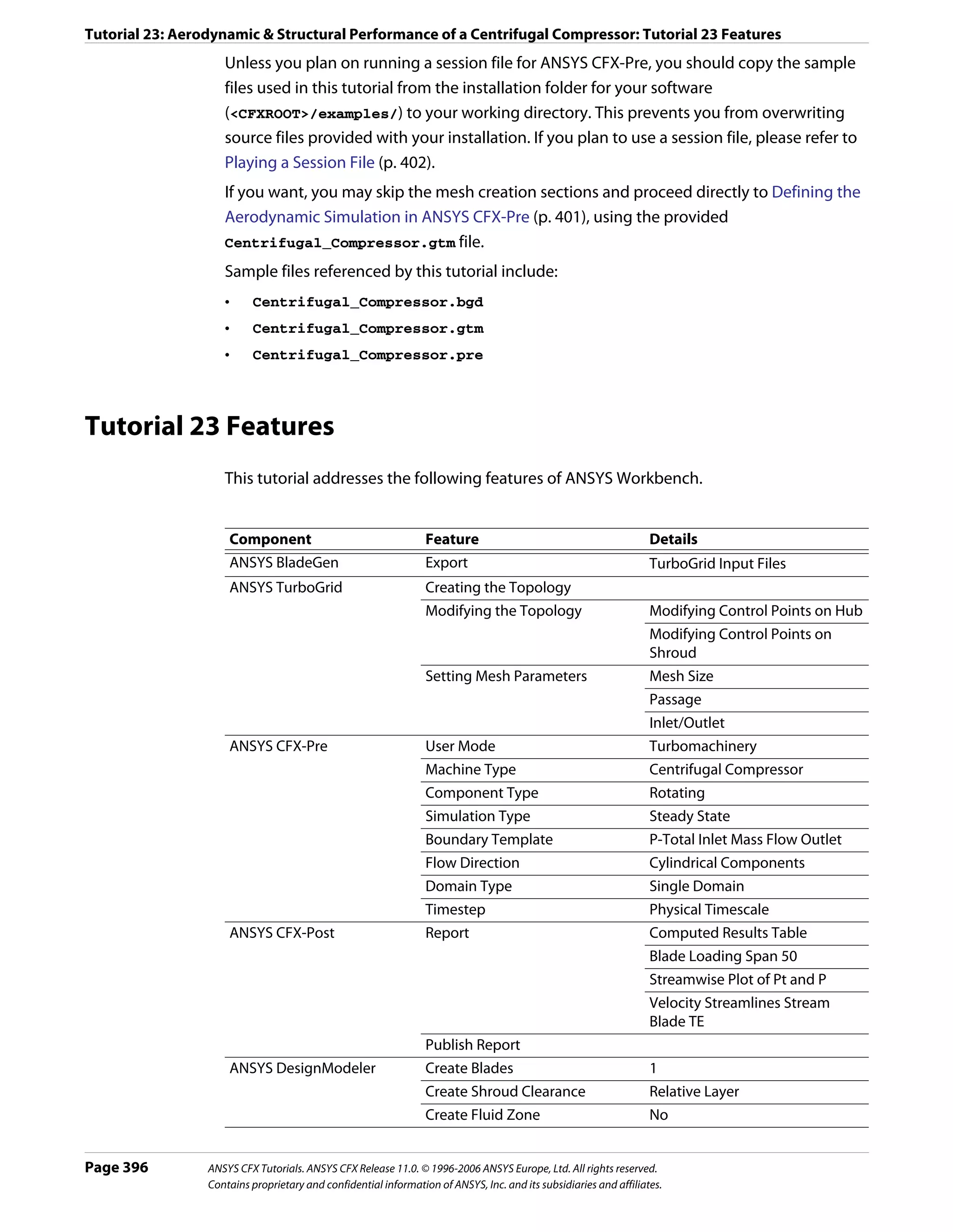
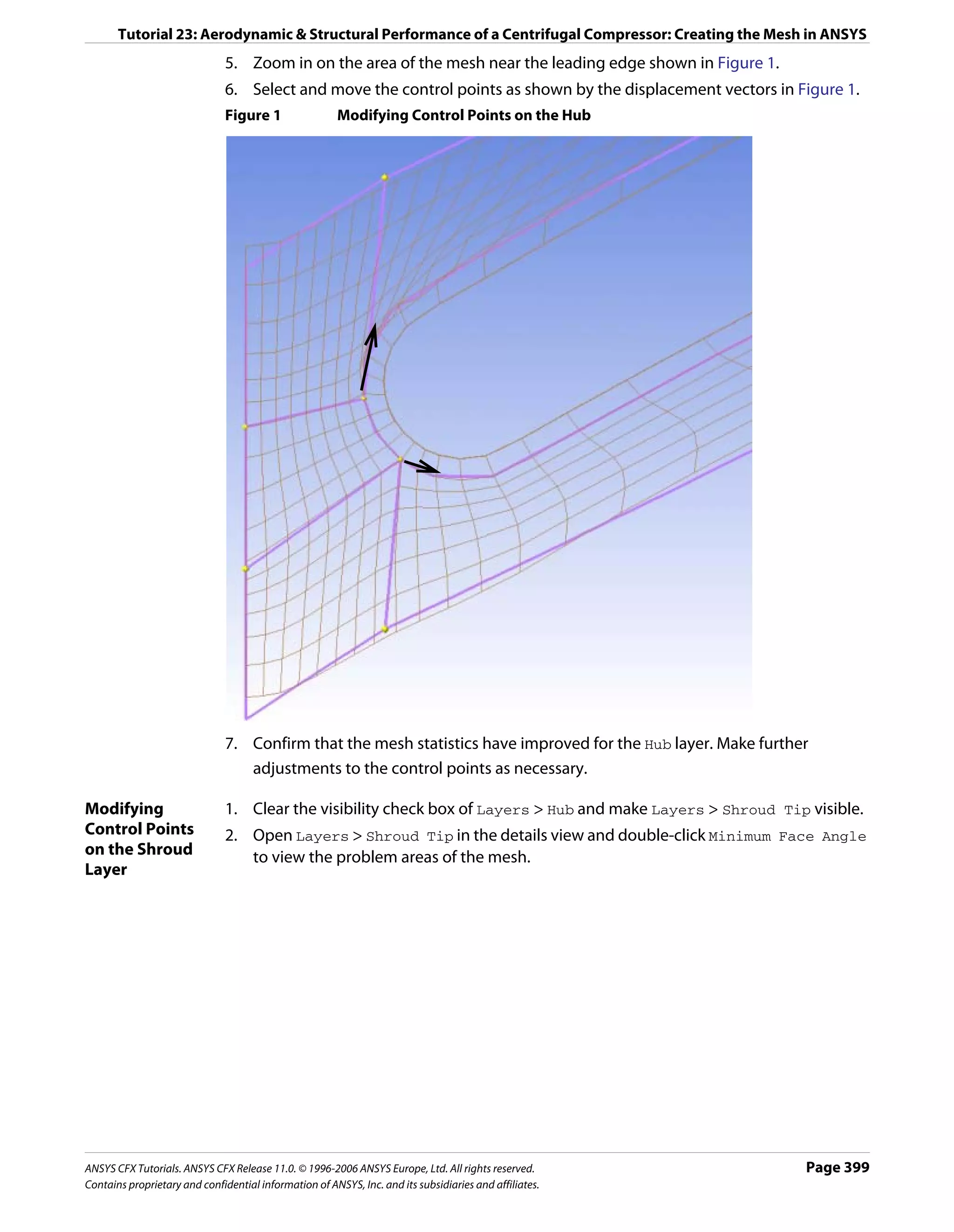


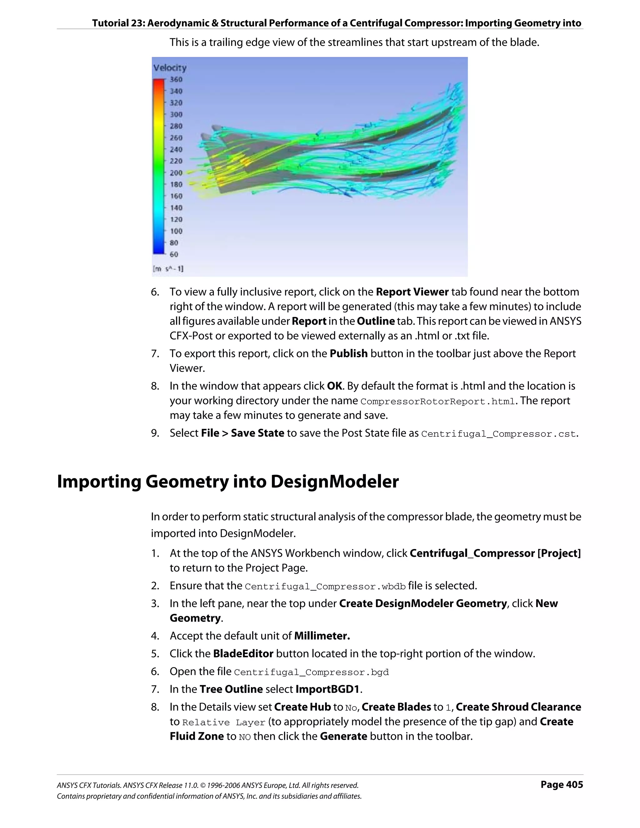


This document provides tutorials for using the ANSYS CFX software to simulate fluid flow and heat transfer. The tutorials cover a range of scenarios including flow through static mixers, injection mixing pipes, and a circular vent. They demonstrate defining simulations, obtaining solutions, and viewing results in ANSYS CFX-Pre, ANSYS CFX-Solver Manager, and ANSYS CFX-Post. The tutorials also illustrate using both standalone and integrated Workbench modes.


![UiPath Automation Suite Installation (Hands-On) [2/3]](https://cdn.slidesharecdn.com/ss_thumbnails/automationsuitecommunitysession2-251015095633-a6d862f1-thumbnail.jpg?width=600ounds&width=560&fit=bounds)


