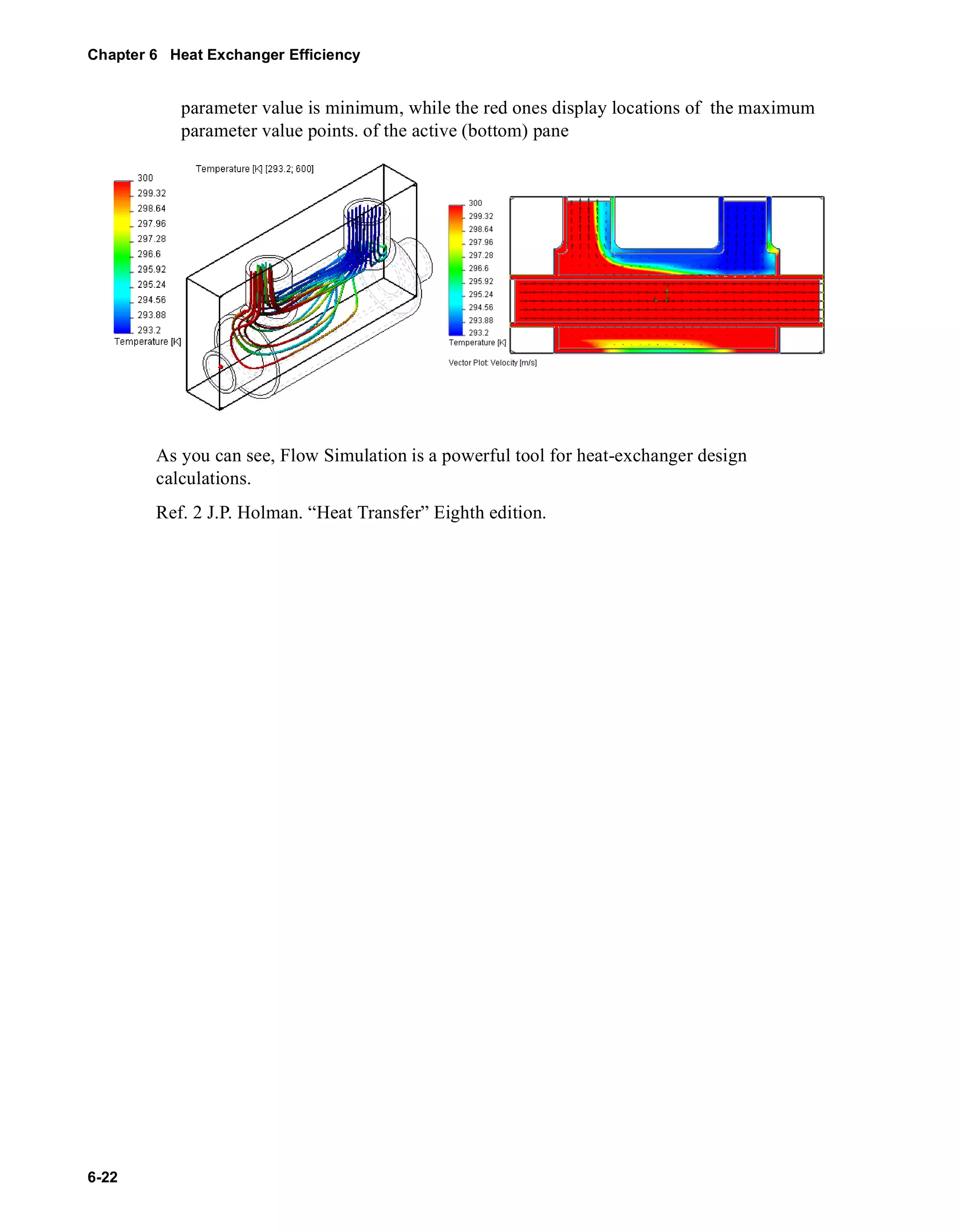
Downloaded 139 times


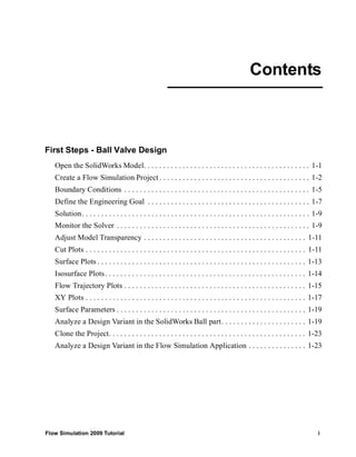


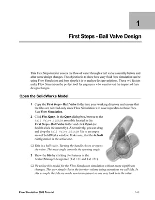
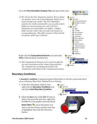


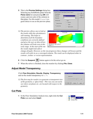
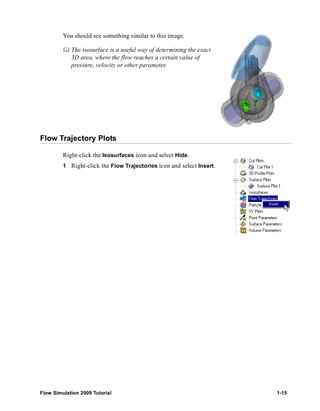
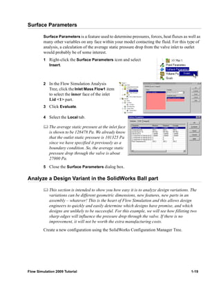
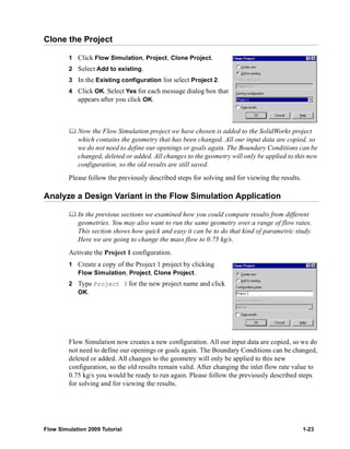

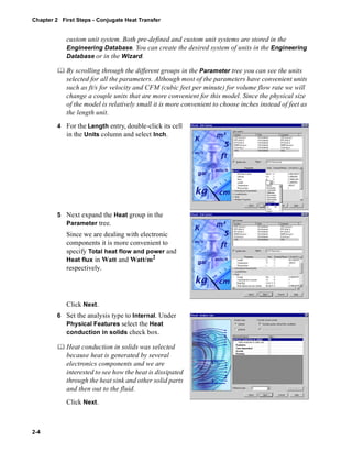

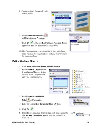
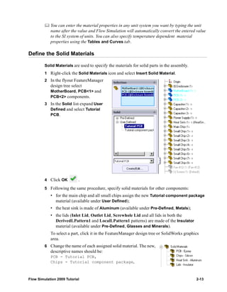

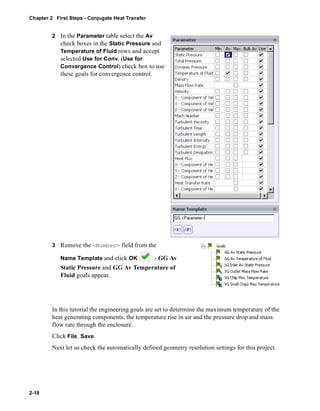
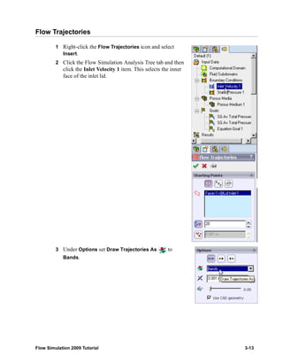
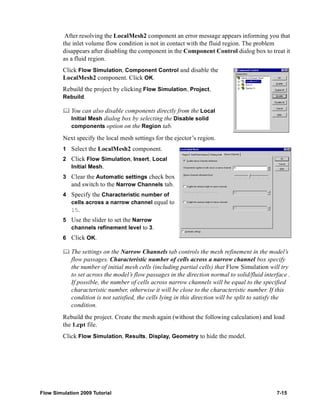
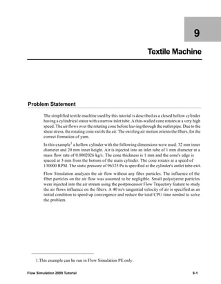
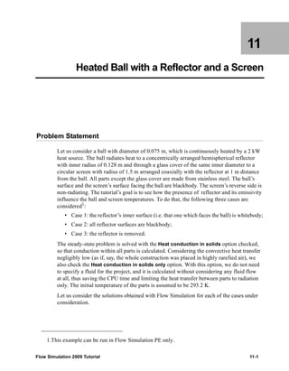
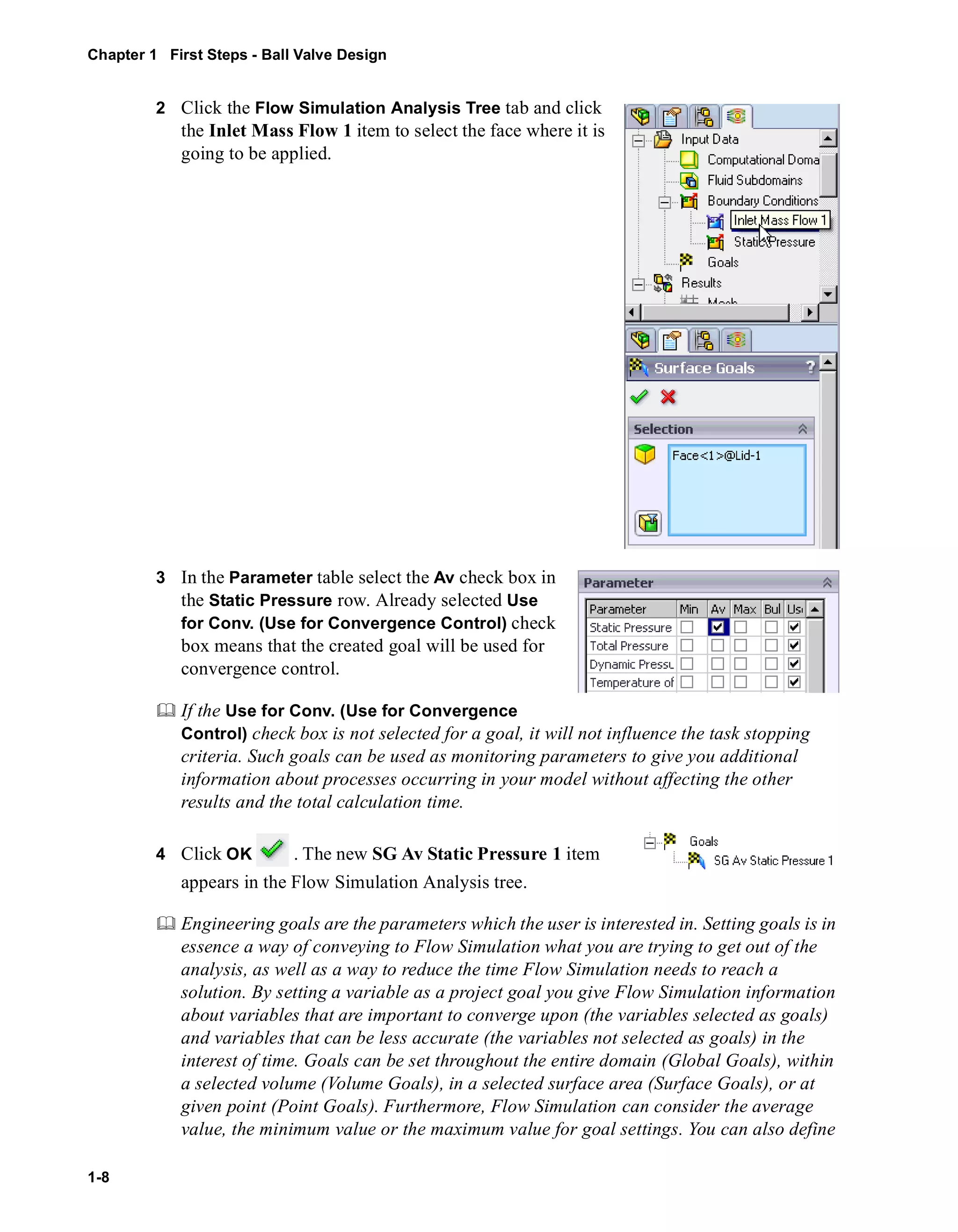
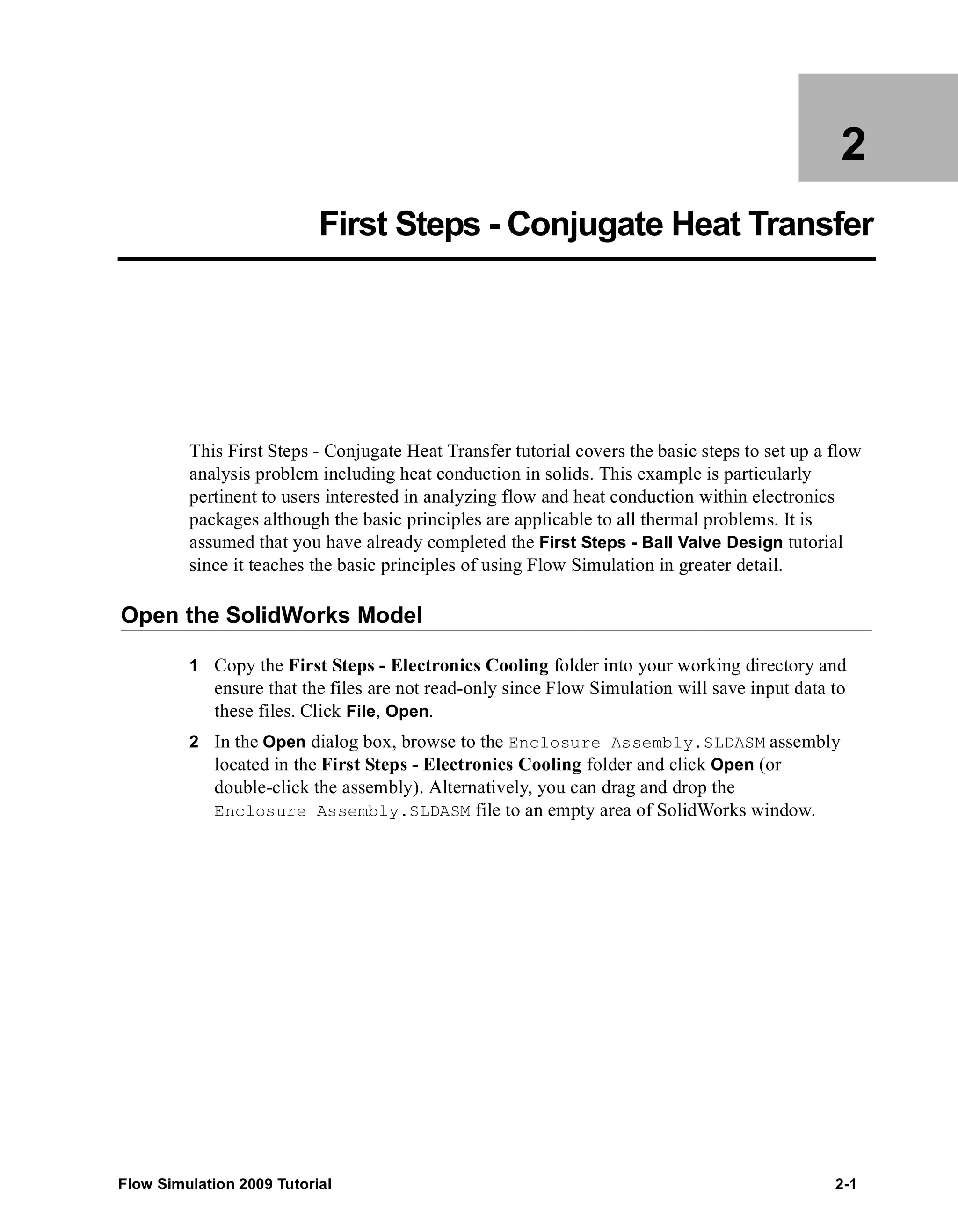
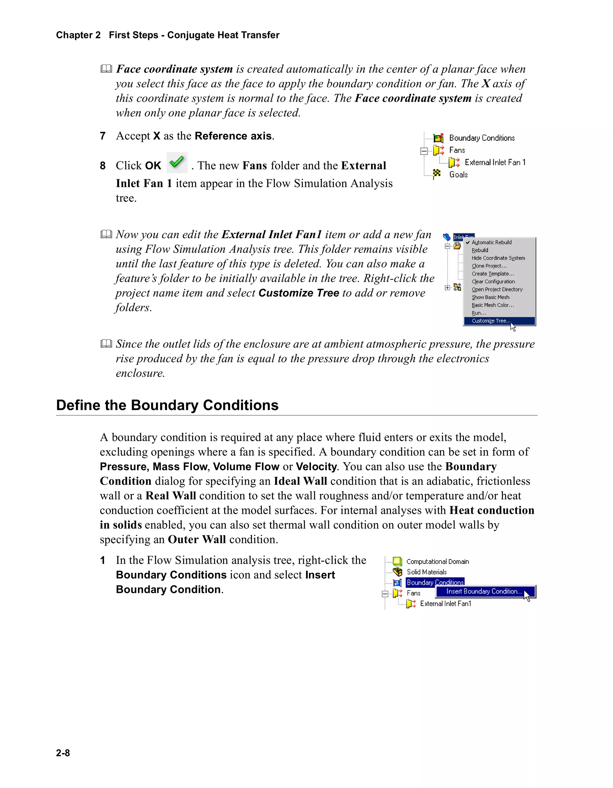
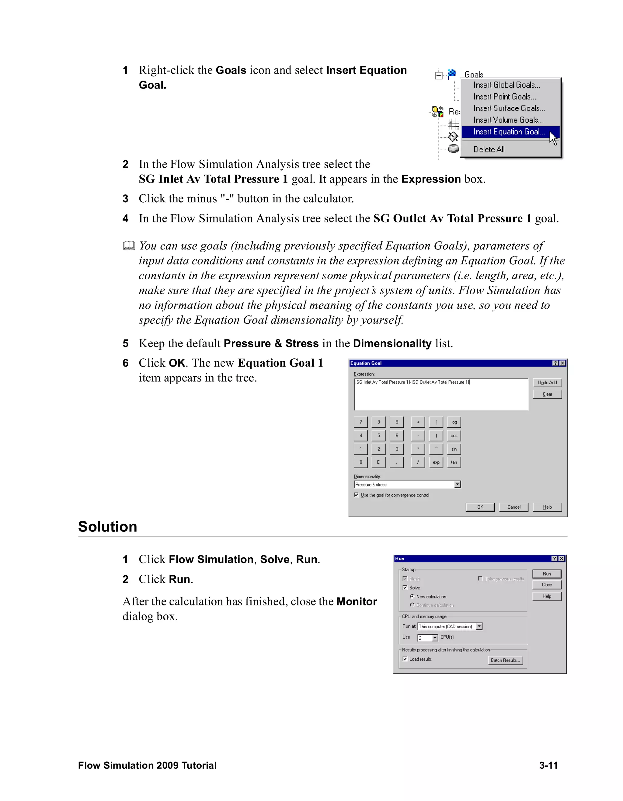
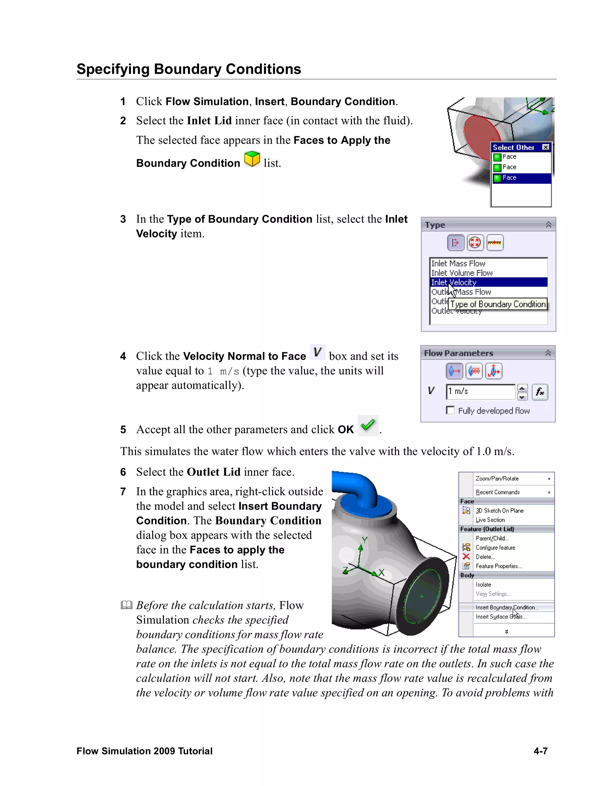
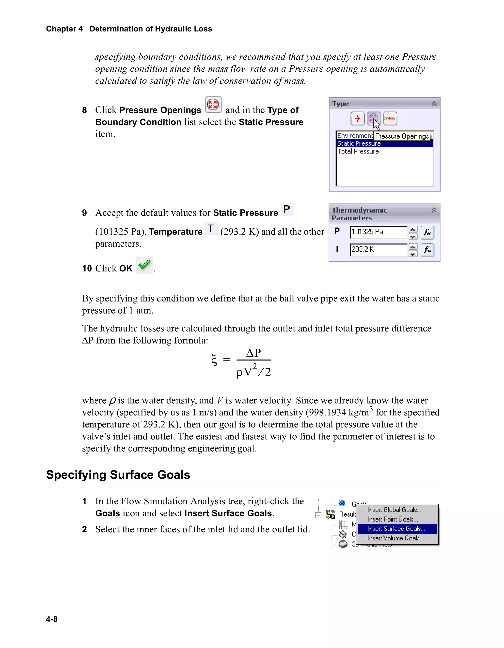
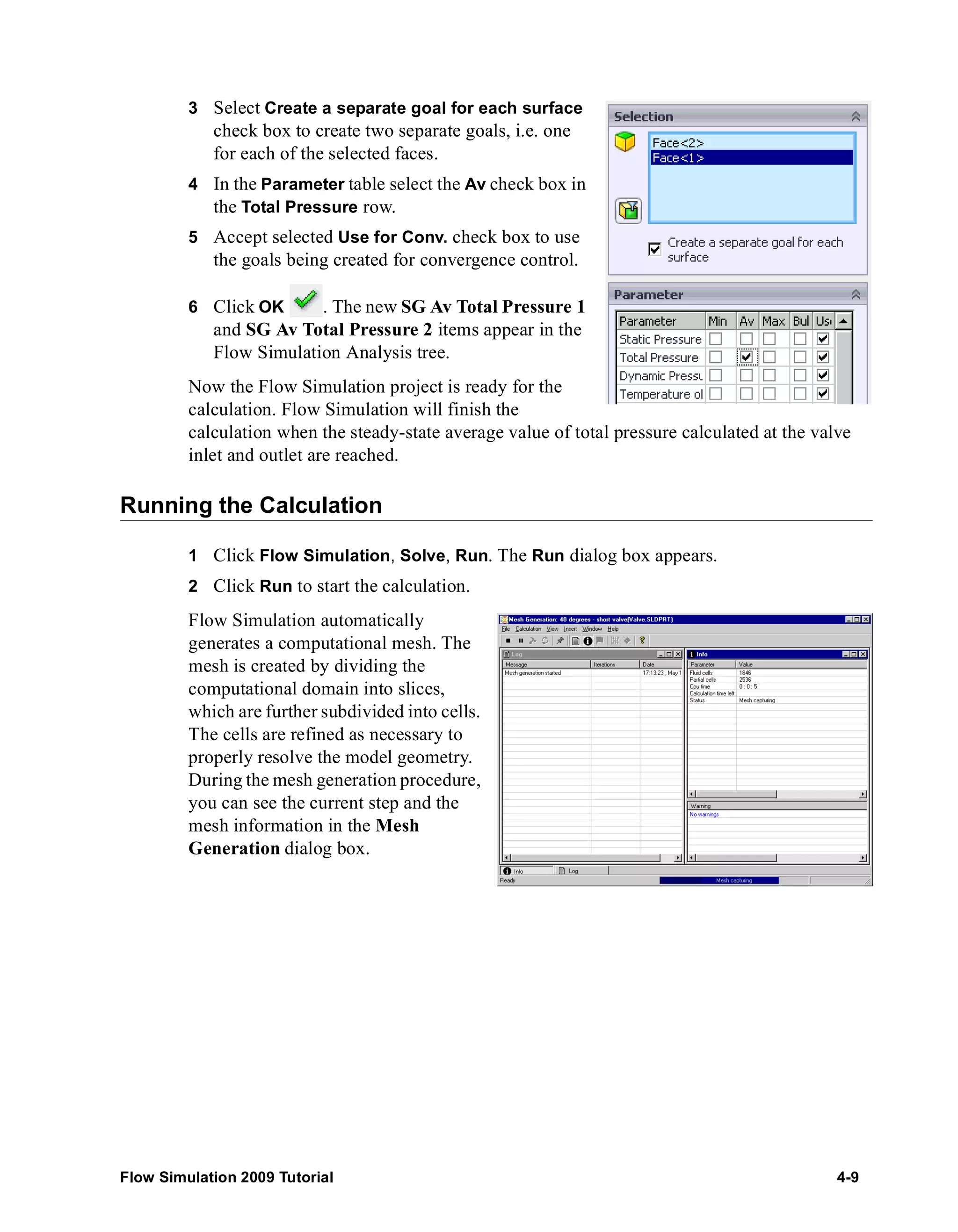
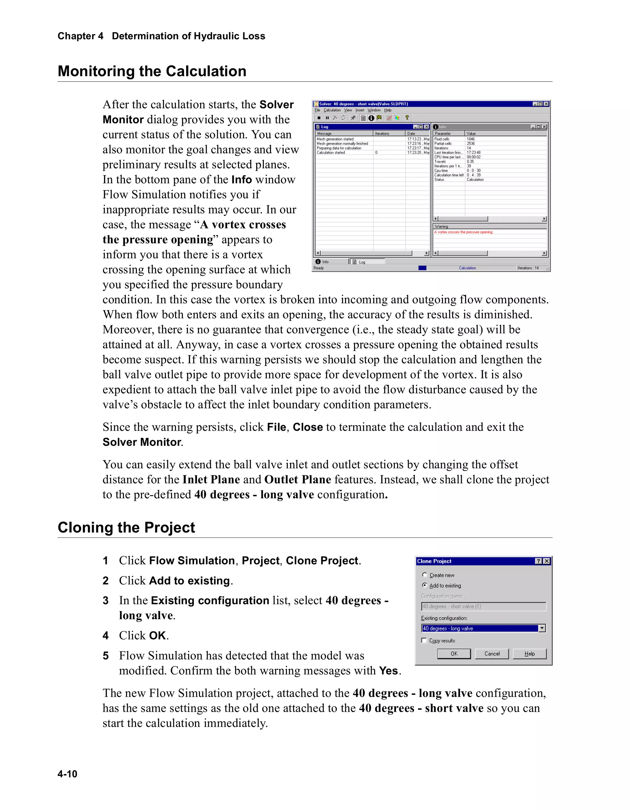
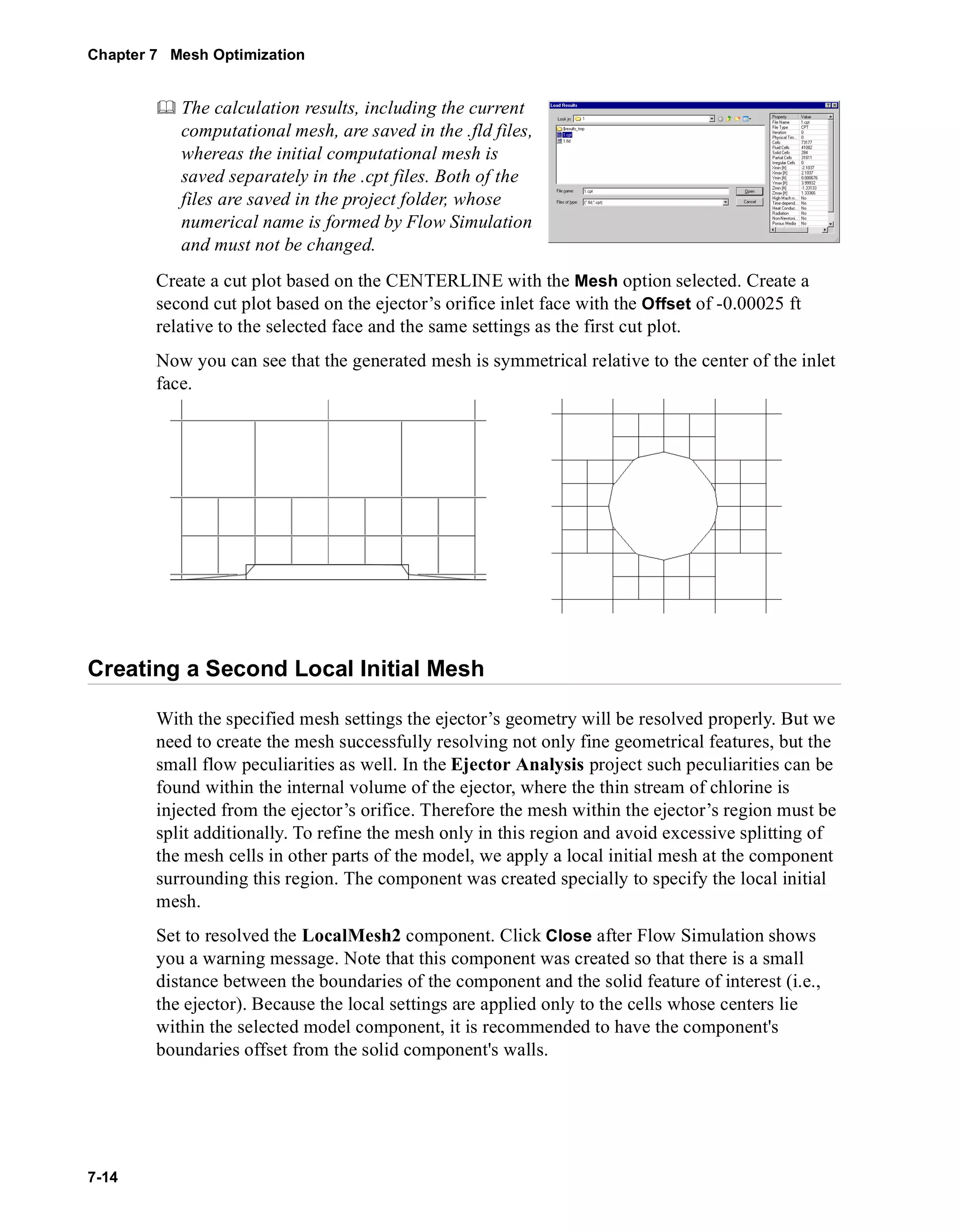
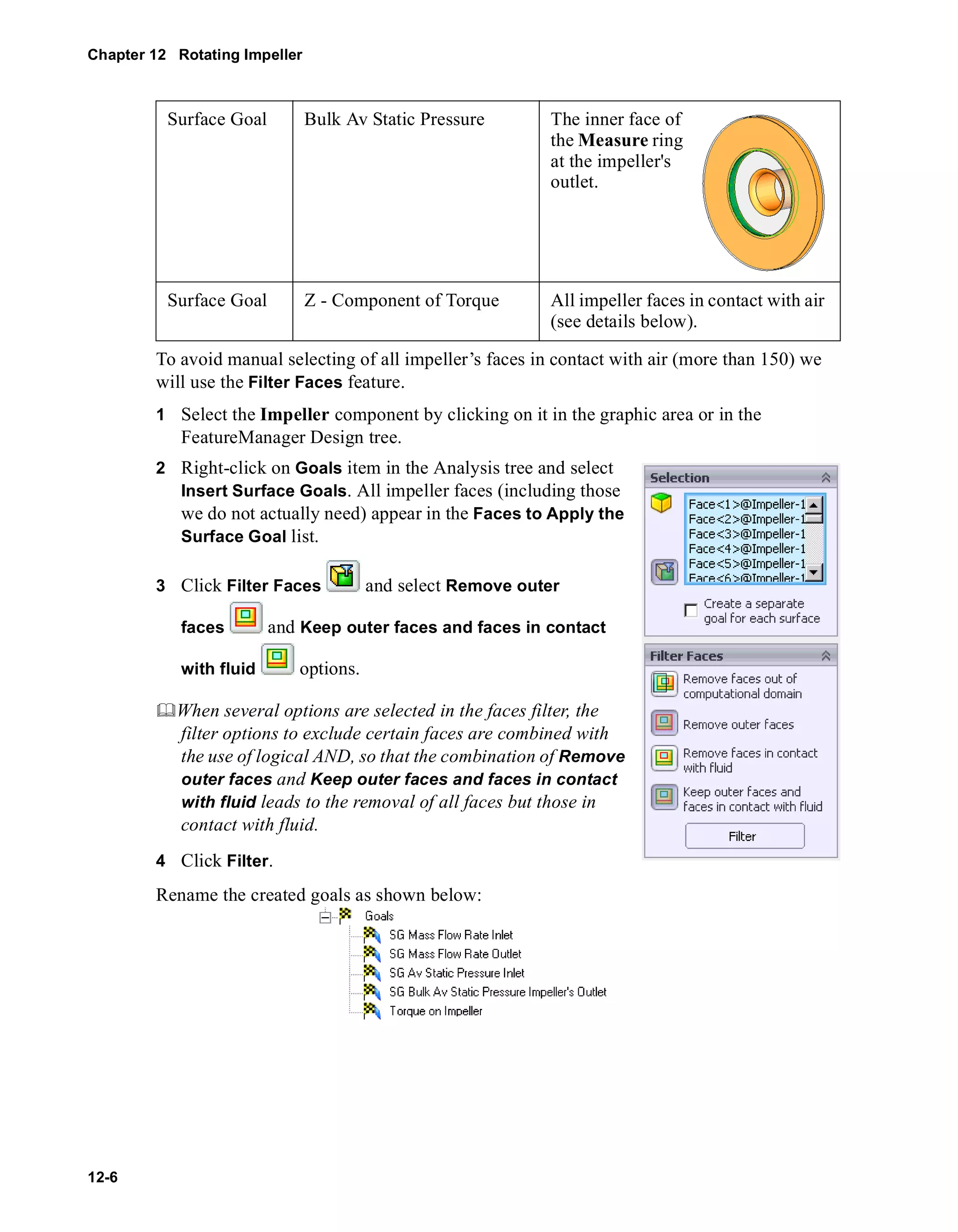
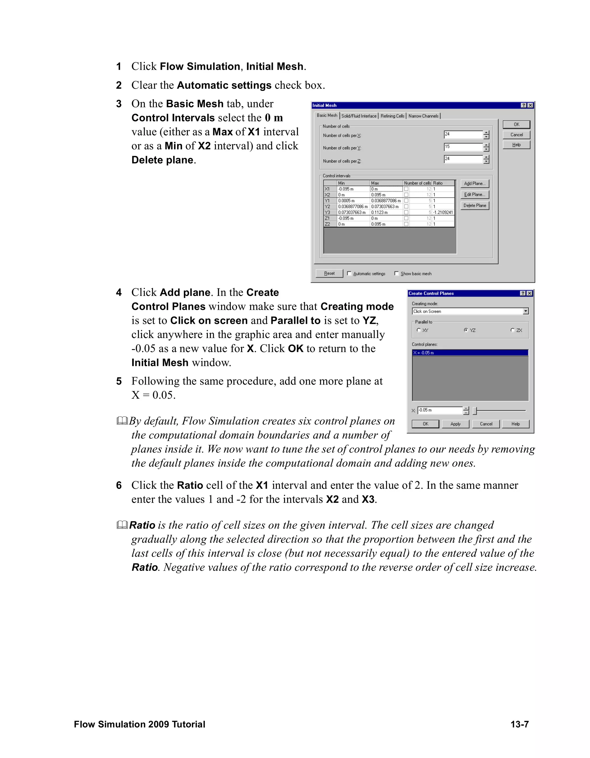
![An Excel spreadsheet with the goal results will open. The first sheet will show a table
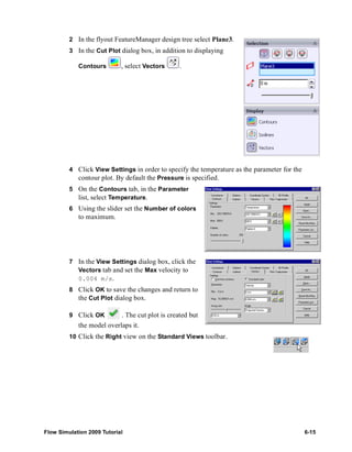
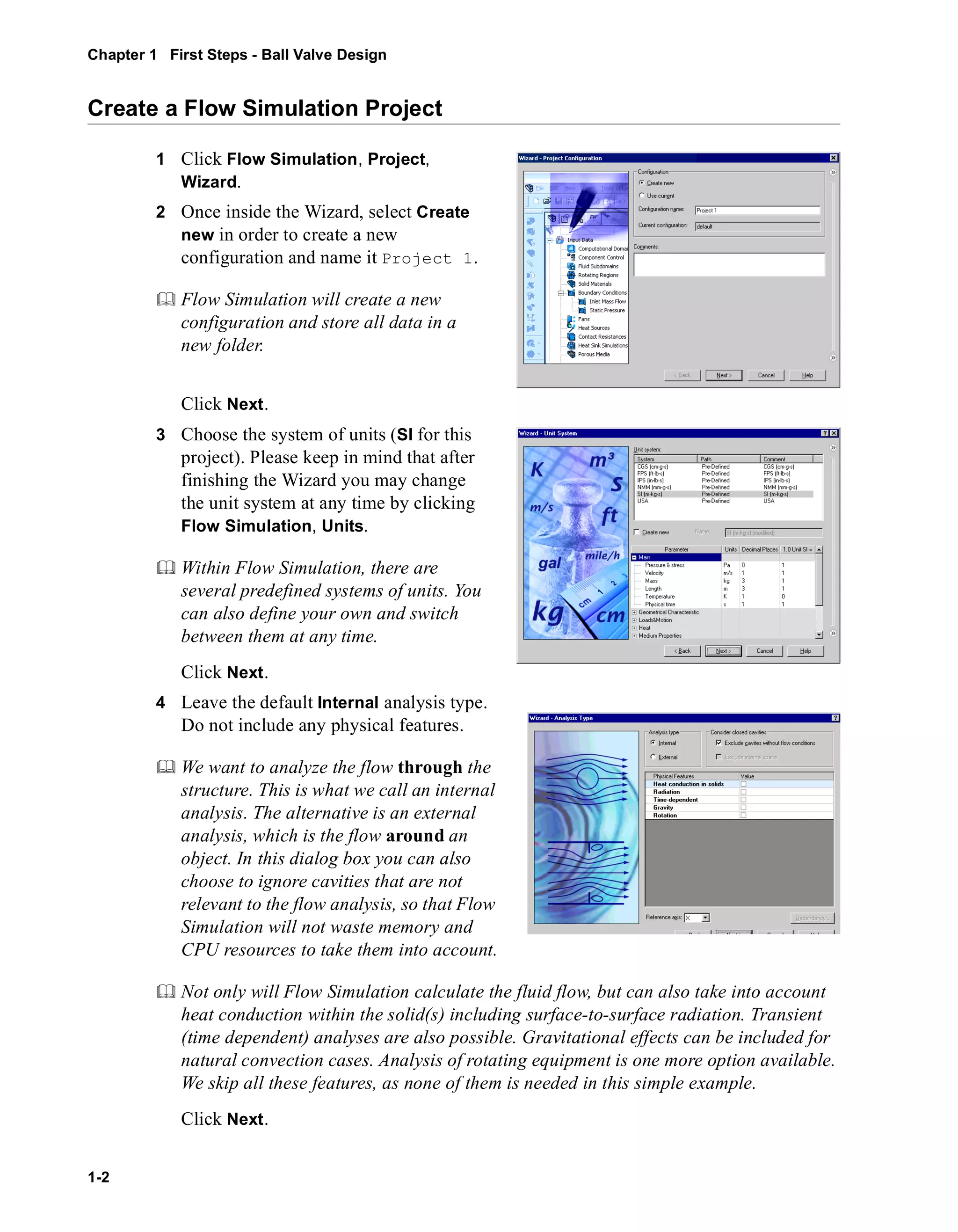
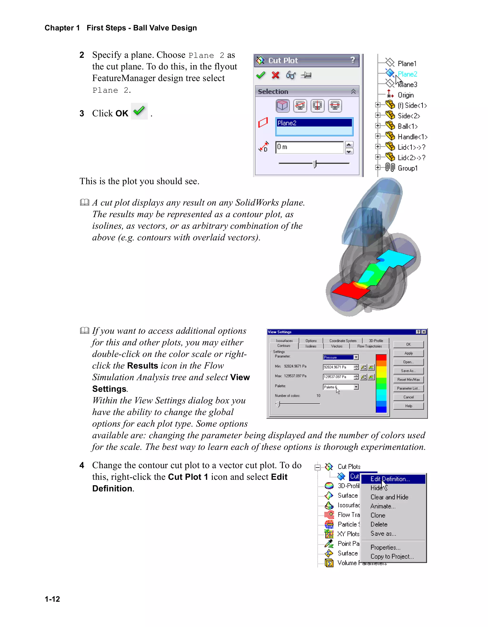
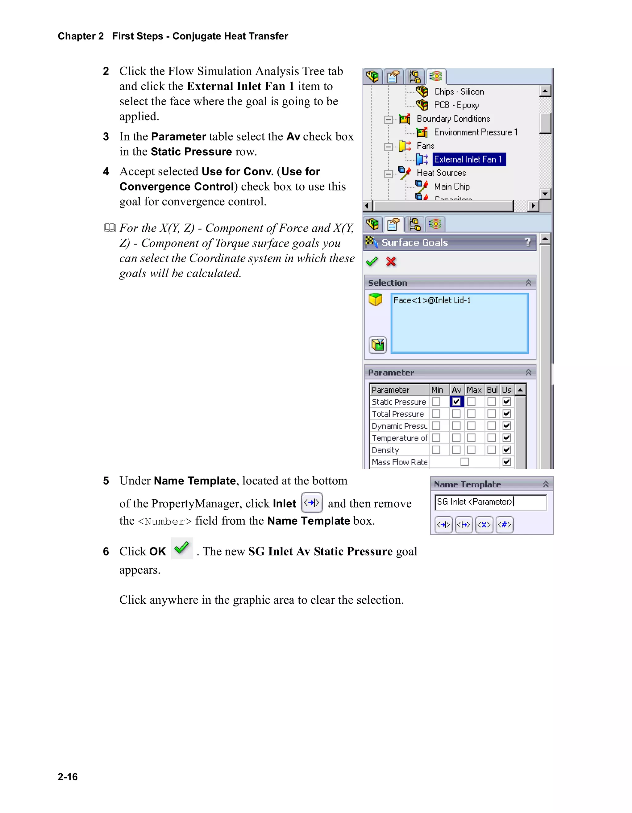
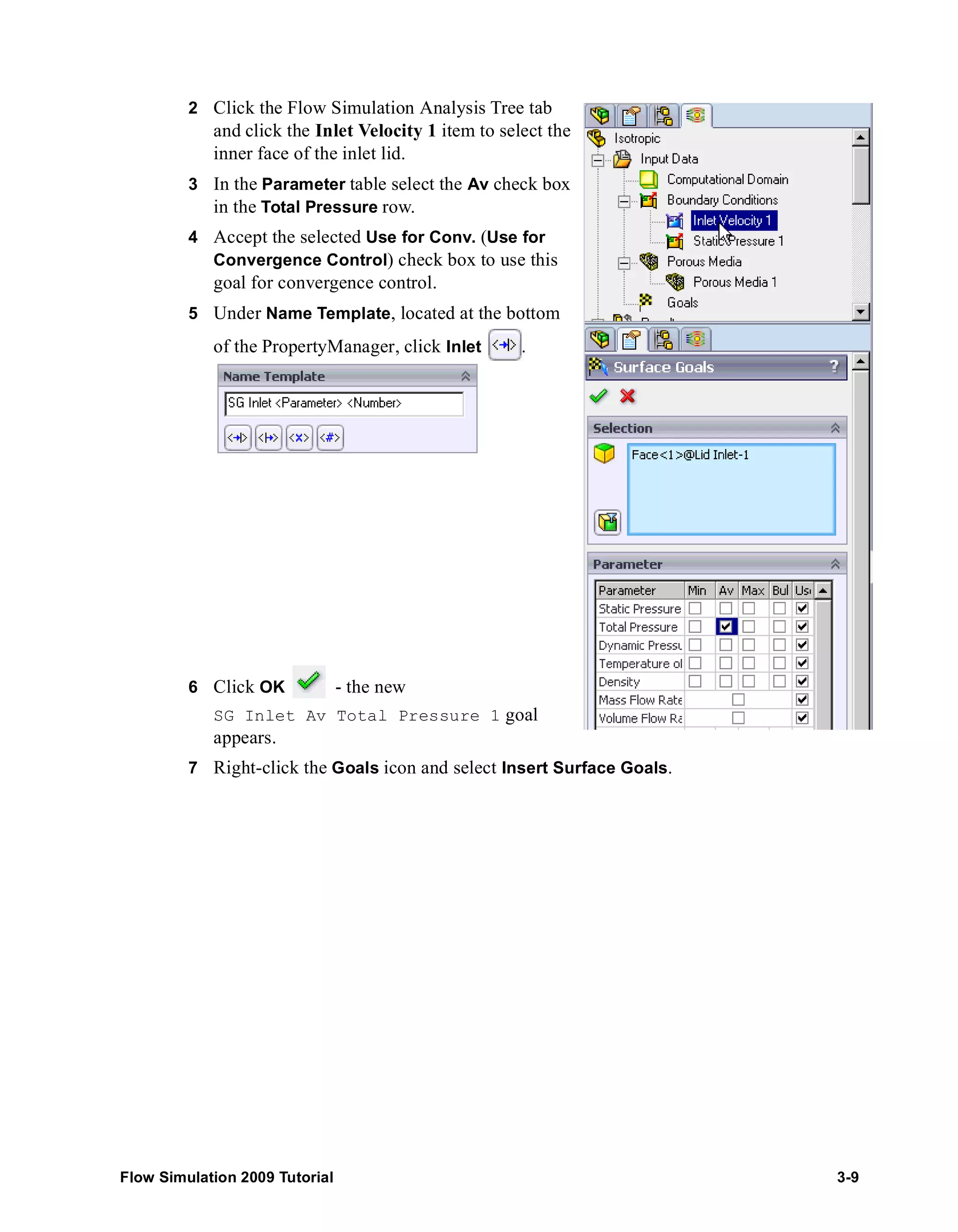
summarizing the goals.
Enclosure Assembly.SLDASM [Inlet Fan (original)]
Goal Name Unit Value Averaged Value Minimum Value Maximum Value Progress [%] Use In Convergence
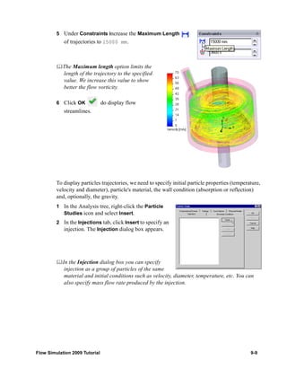
GG Av Static Pressure [lbf/in^2] 14.69678696 14.69678549 14.69678314 14.69678772 100 Yes
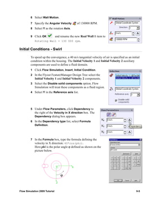
SG Inlet Av Static Pressure [lbf/in^2] 14.69641185 14.69641047 14.69640709 14.69641418 100 Yes
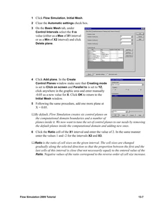
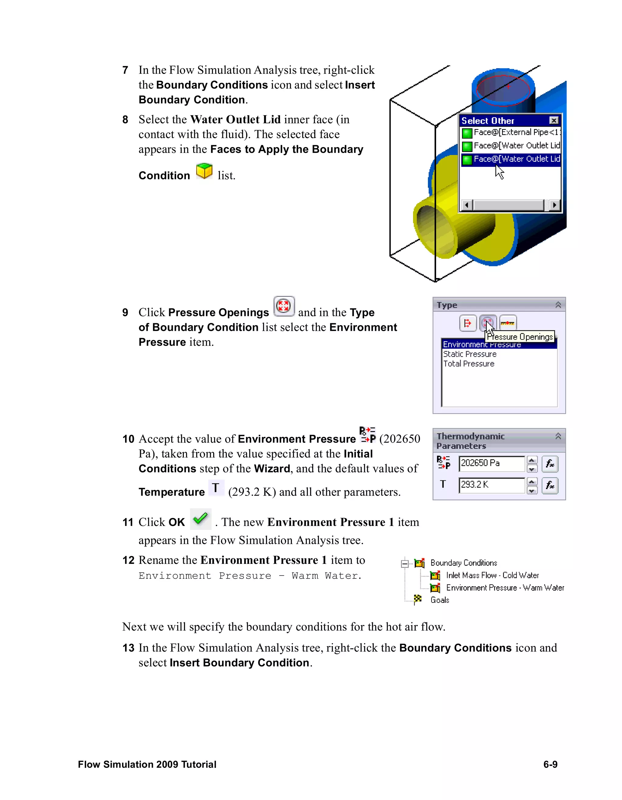
GG Av Temperature of Fluid [°F] 61.7814683 61.76016724 61.5252449 61.86764155 100 Yes
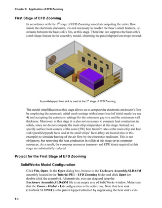
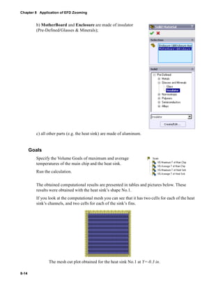
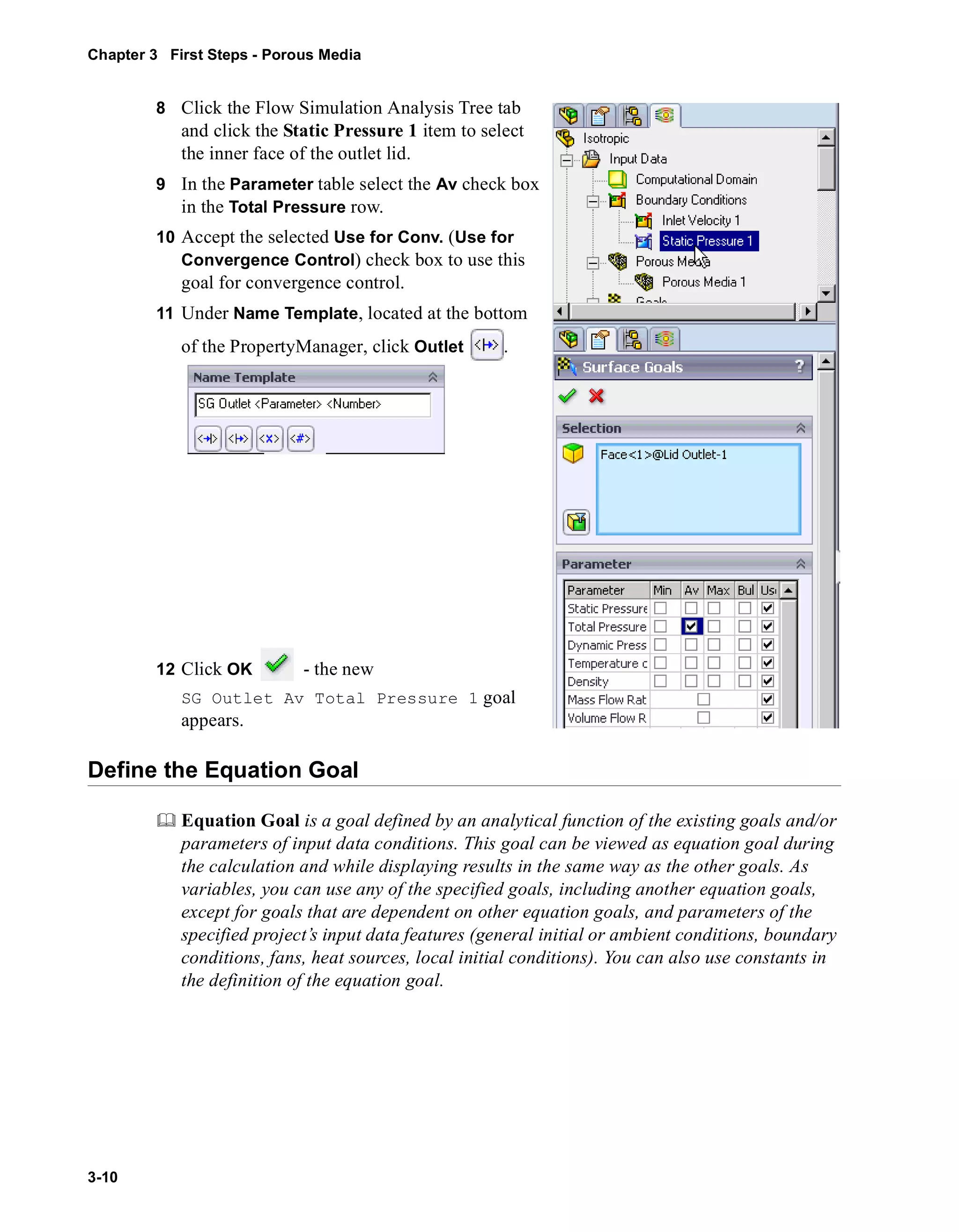
SG Outlet Mass Flow Rate [lb/s] -0.007306292 -0.007306111 -0.007306913 -0.007303663 100 Yes
VG Small Chips Max Temp [°F] 91.5523903 90.97688632 90.09851988 91.5523903 100 Yes
VG Chip Max Temperature [°F] 88.51909612 88.43365626 88.29145322 88.57515562 100 Yes
You can see that the maximum temperature in the main chip is about 88 °F, and the
maximum temperature over the small chips is about 91 °F.
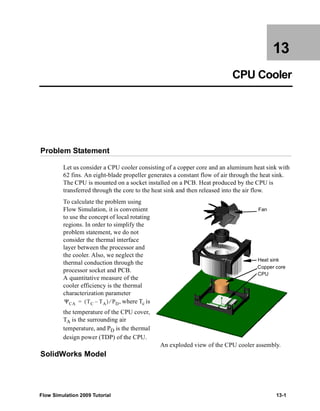
Goal progress bar is a qualitative and quantitative characteristic of the goal
convergence process. When Flow Simulation analyzes the goal convergence, it
calculates the goal dispersion defined as the difference between the maximum and
minimum goal values over the analysis interval reckoned from the last iteration and
compares this dispersion with the goal's convergence criterion dispersion, either
specified by you or automatically determined by Flow Simulation as a fraction of the
goal's physical parameter dispersion over the computational domain. The percentage
of the goal's convergence criterion dispersion to the goal's real dispersion over the
analysis interval is shown in the goal's convergence progress bar (when the goal's real
dispersion becomes equal or smaller than the goal's convergence criterion dispersion,
the progress bar is replaced by word "Achieved"). Naturally, if the goal's real
dispersion oscillates, the progress bar oscillates also, moreover, when a hard problem
is solved, it can noticeably regress, in particular from the "achieved" level. The
calculation can finish if the iterations (in travels) required for finishing the calculation
have been performed, or if the goal convergence criteria are satisfied before
performing the required number of iterations. You can specify other finishing
conditions at your discretion.
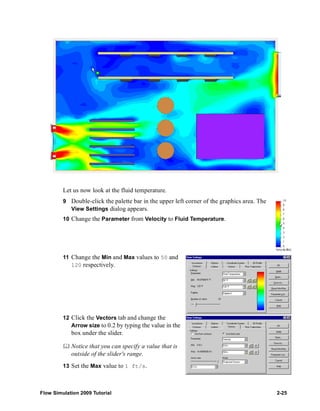
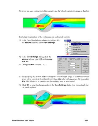
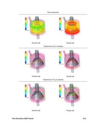
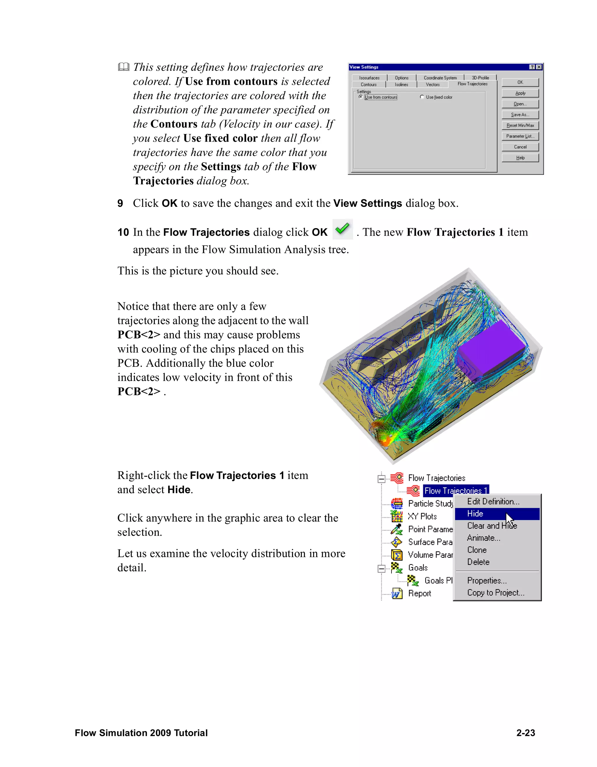
To analyze the results in more detail let us use the various Flow Simulation
post-processing tools. The best method for the visualization of how the fluid flows inside
the enclosure is to create flow trajectories.
Flow Simulation 2009 Tutorial 2-21](https://image.slidesharecdn.com/swflowsimulation2009tutorial-141007202601-conversion-gate02/85/Sw-flowsimulation-2009-tutorial-65-320.jpg)


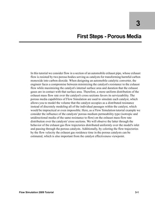

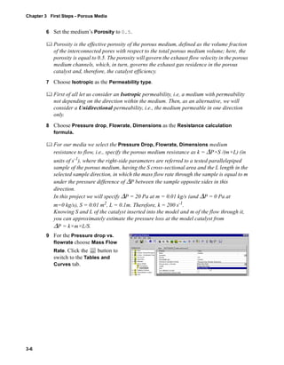


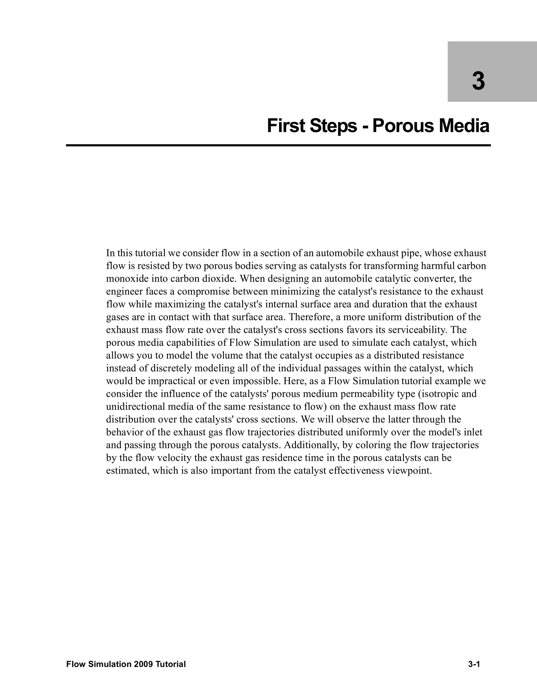
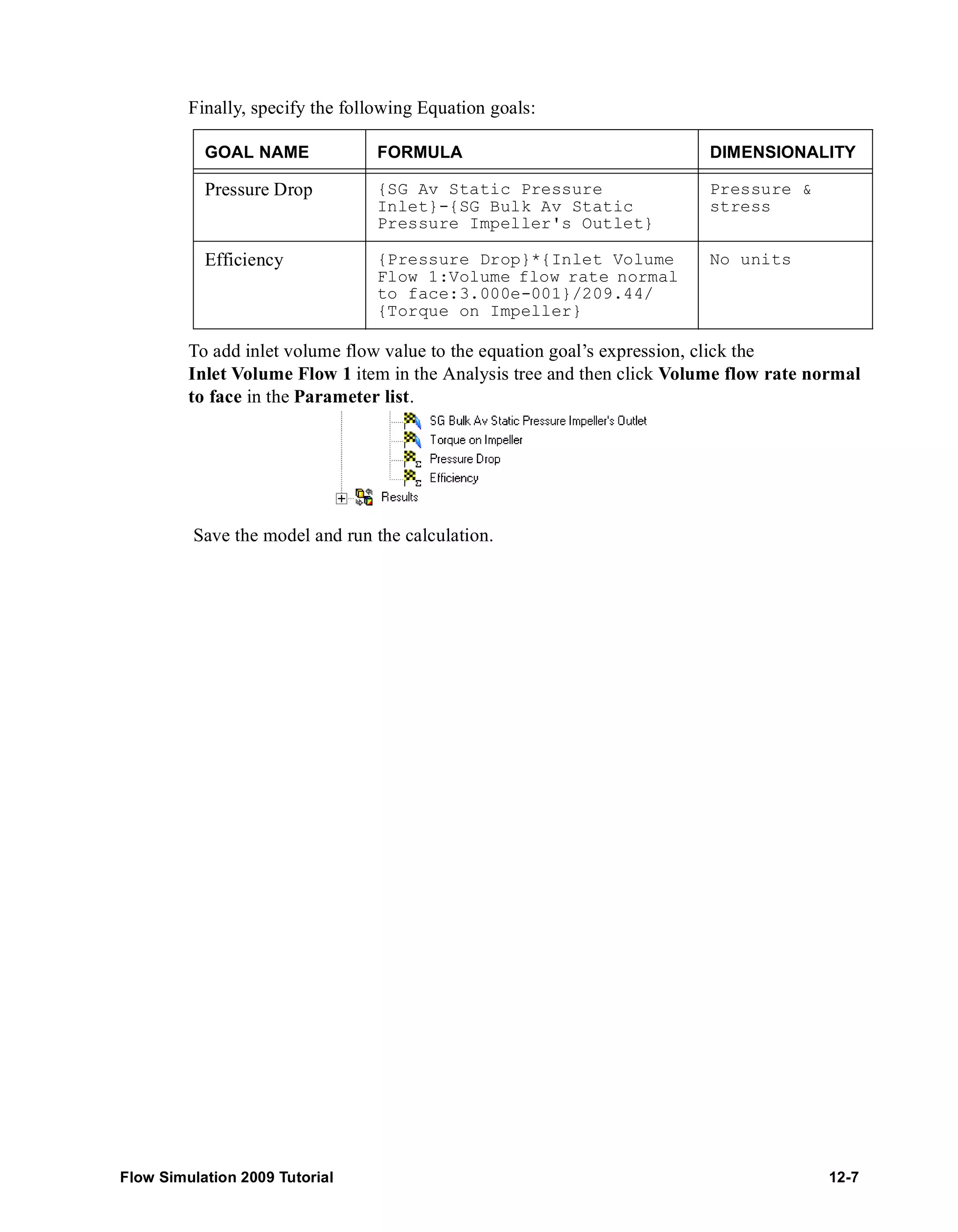
![Chapter 3 First Steps - Porous Media
Viewing the Goals
3-12
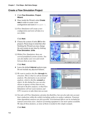
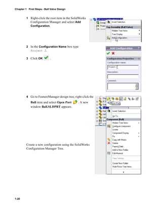
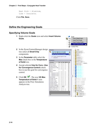
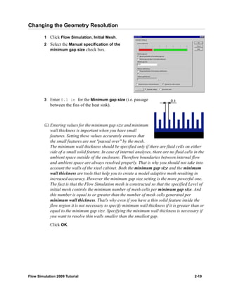
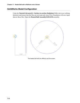
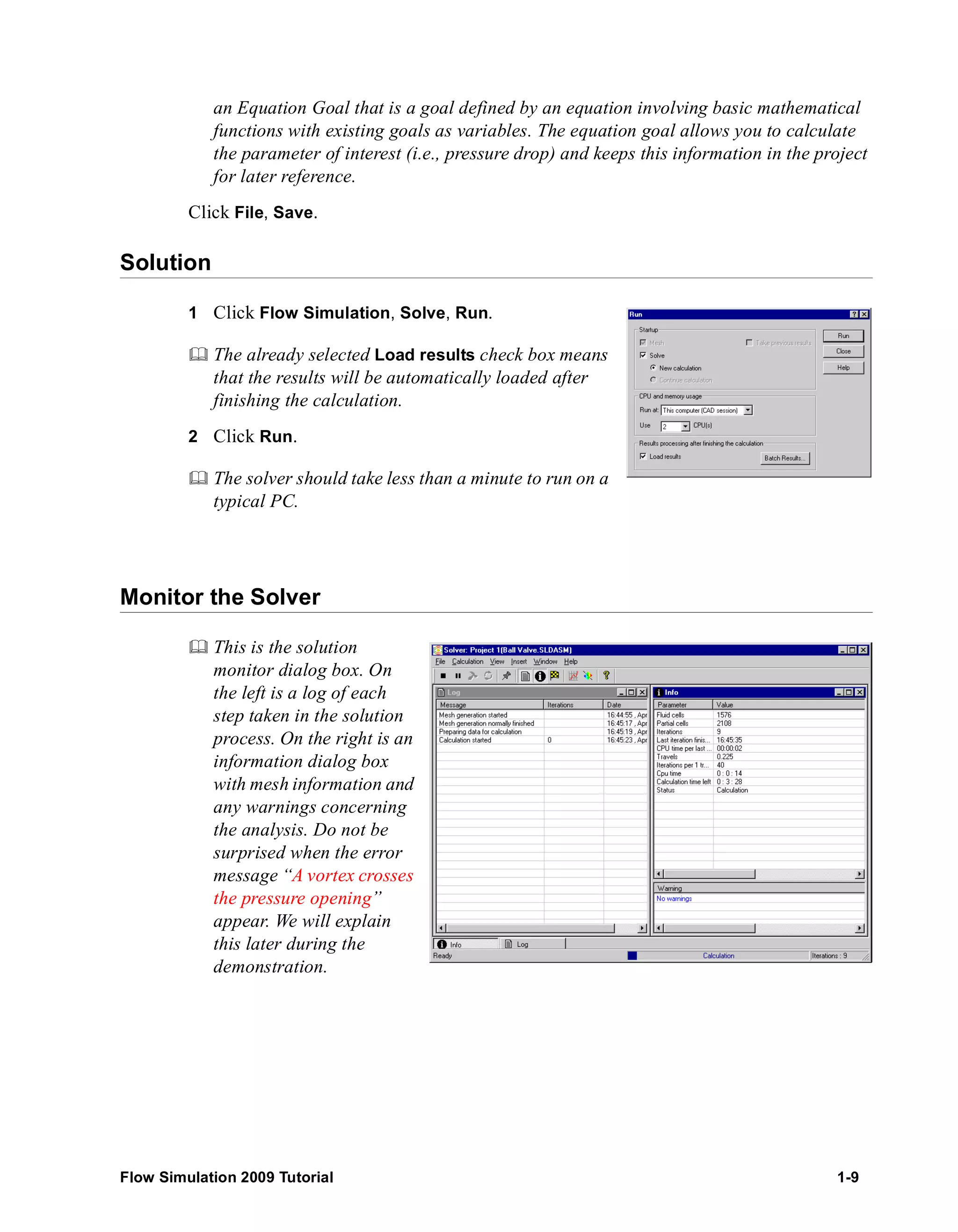
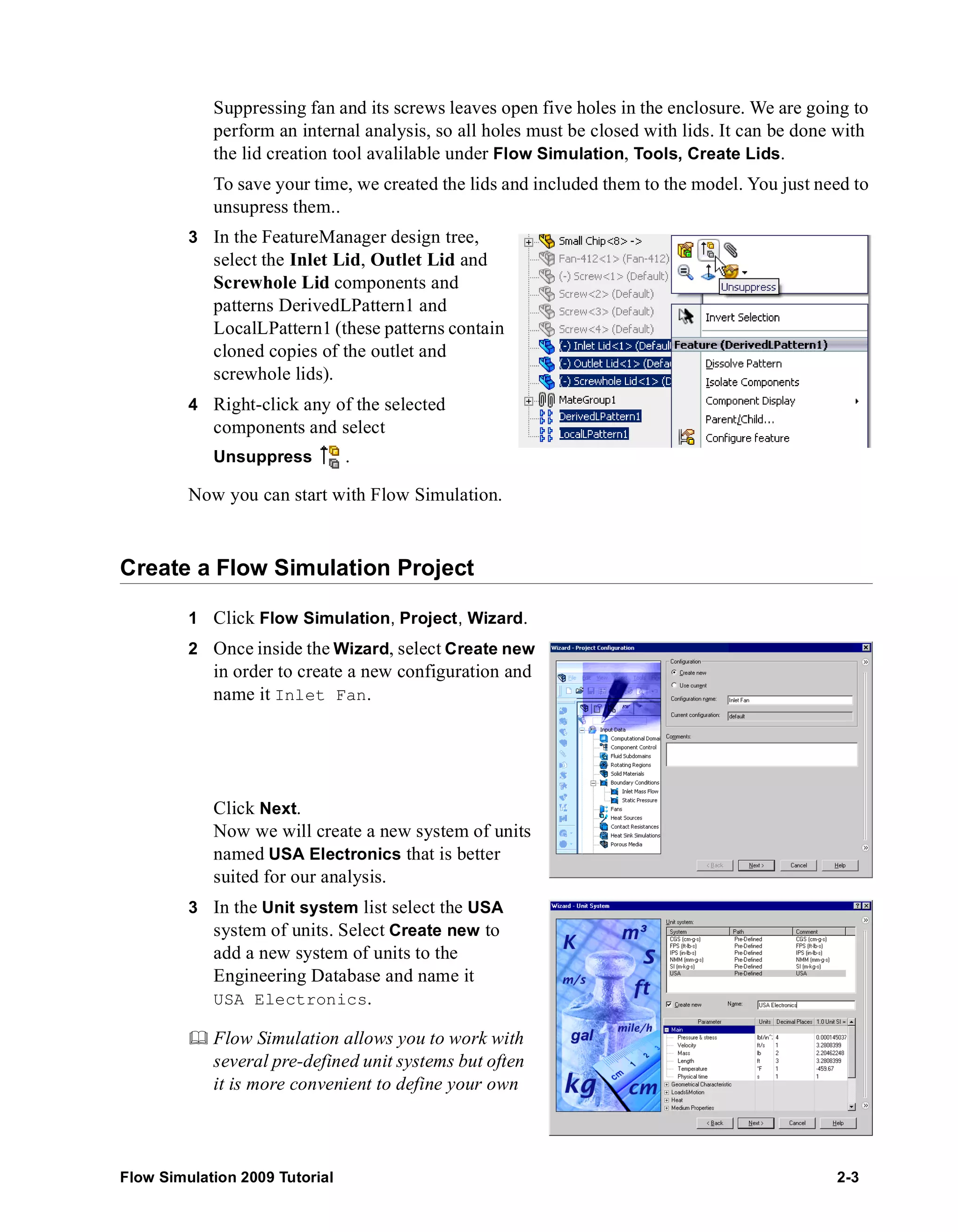
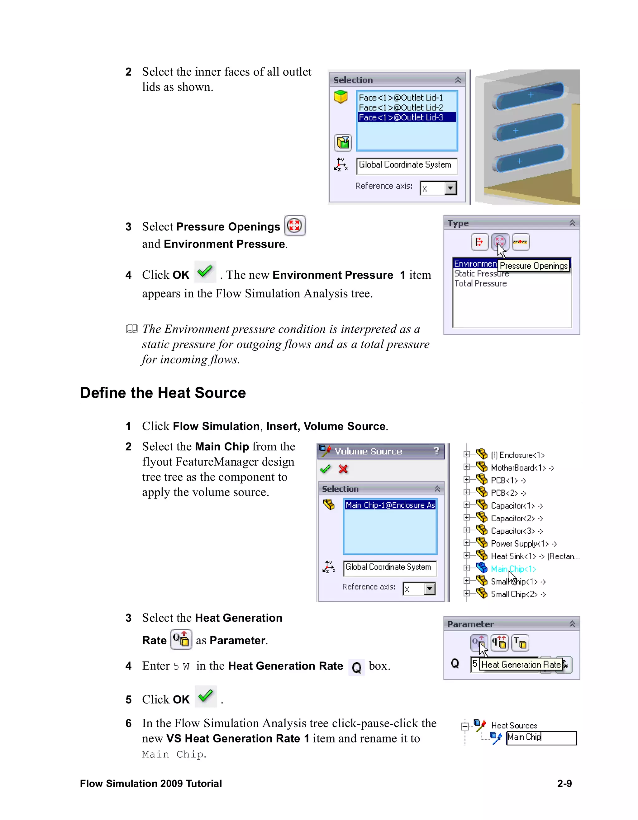
1 Right-click the Goals icon under Results and select Insert.
2 Select the Equation Goal 1 in the Goals
dialog box.
3 Click OK.
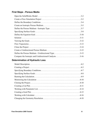
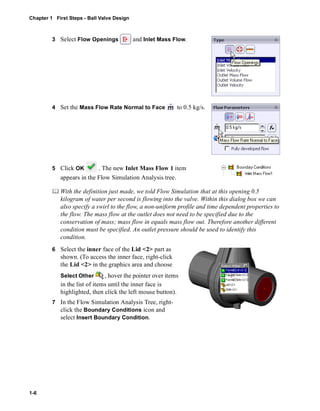
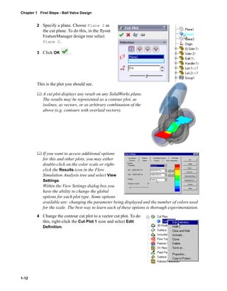
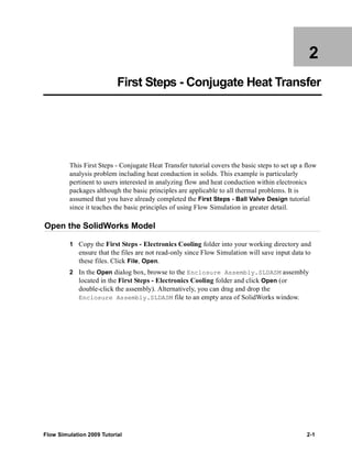
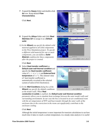
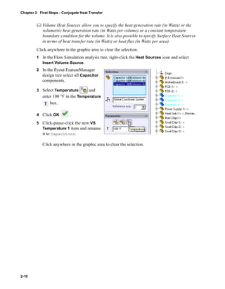
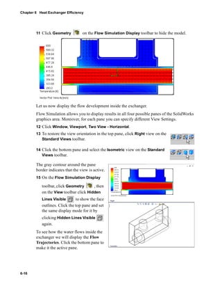
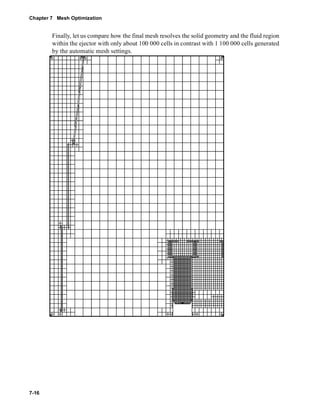
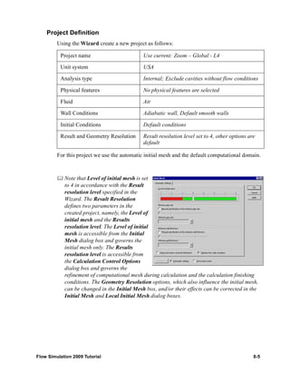
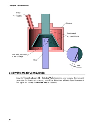
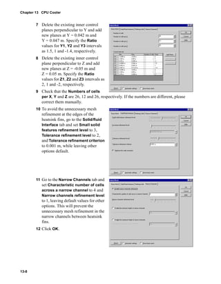
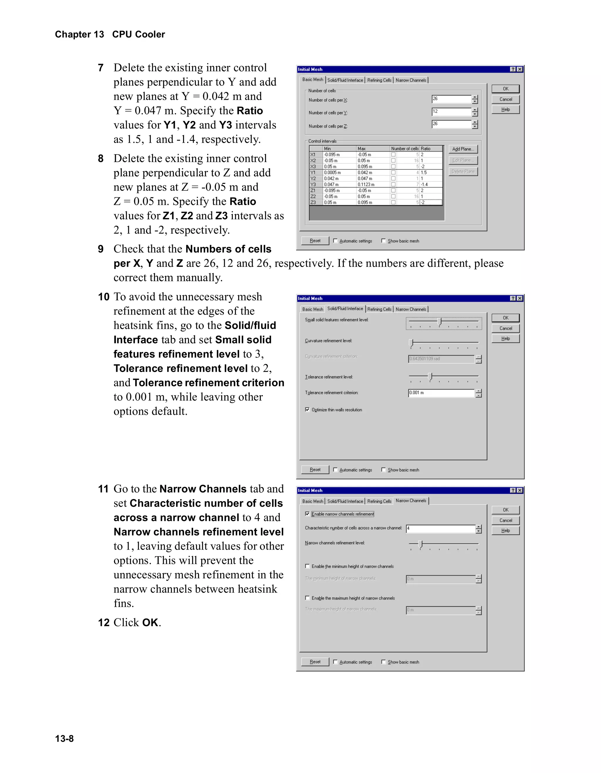
An Excel spreadsheet with the goal results will
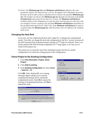
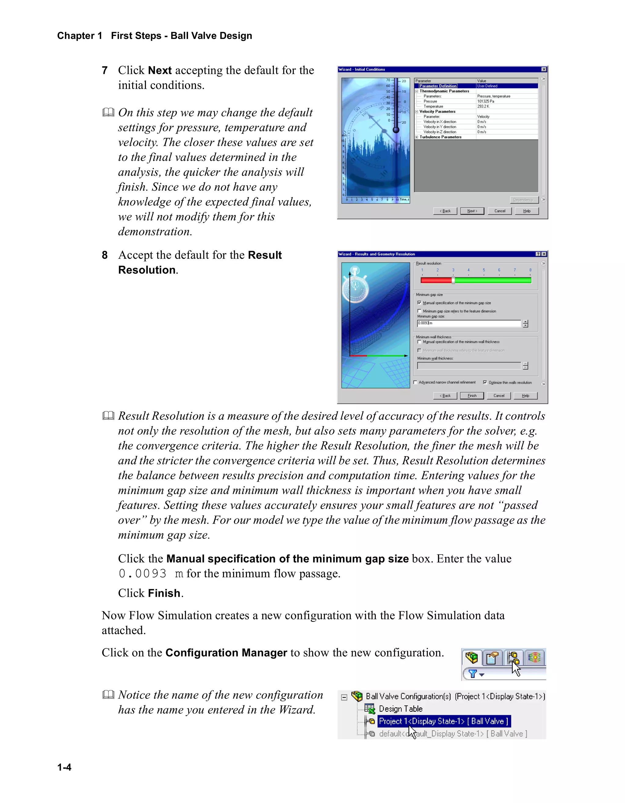
open. The first sheet will contain a table
presenting the final values of the goal.
You can see that the total pressure drop is about 120 Pa.
Catalyst.SLDASM [Isotropic]
Goal Name Unit Value Averaged Value Minimum Value Maximum Value Progress [%] Use In Convergence
Equation Goal 1 [Pa] 120.0326909 121.774802 120.0326909 124.432896 100 Yes
To see the non-uniformity of the mass flow rate distribution over a catalyst’s cross section,
we will display flow trajectories with start points distributed uniformly across the inlet.](https://image.slidesharecdn.com/swflowsimulation2009tutorial-141007202601-conversion-gate02/85/Sw-flowsimulation-2009-tutorial-86-320.jpg)
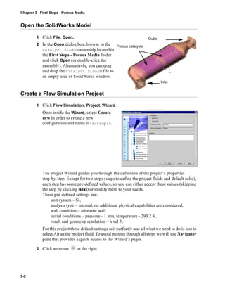
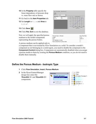
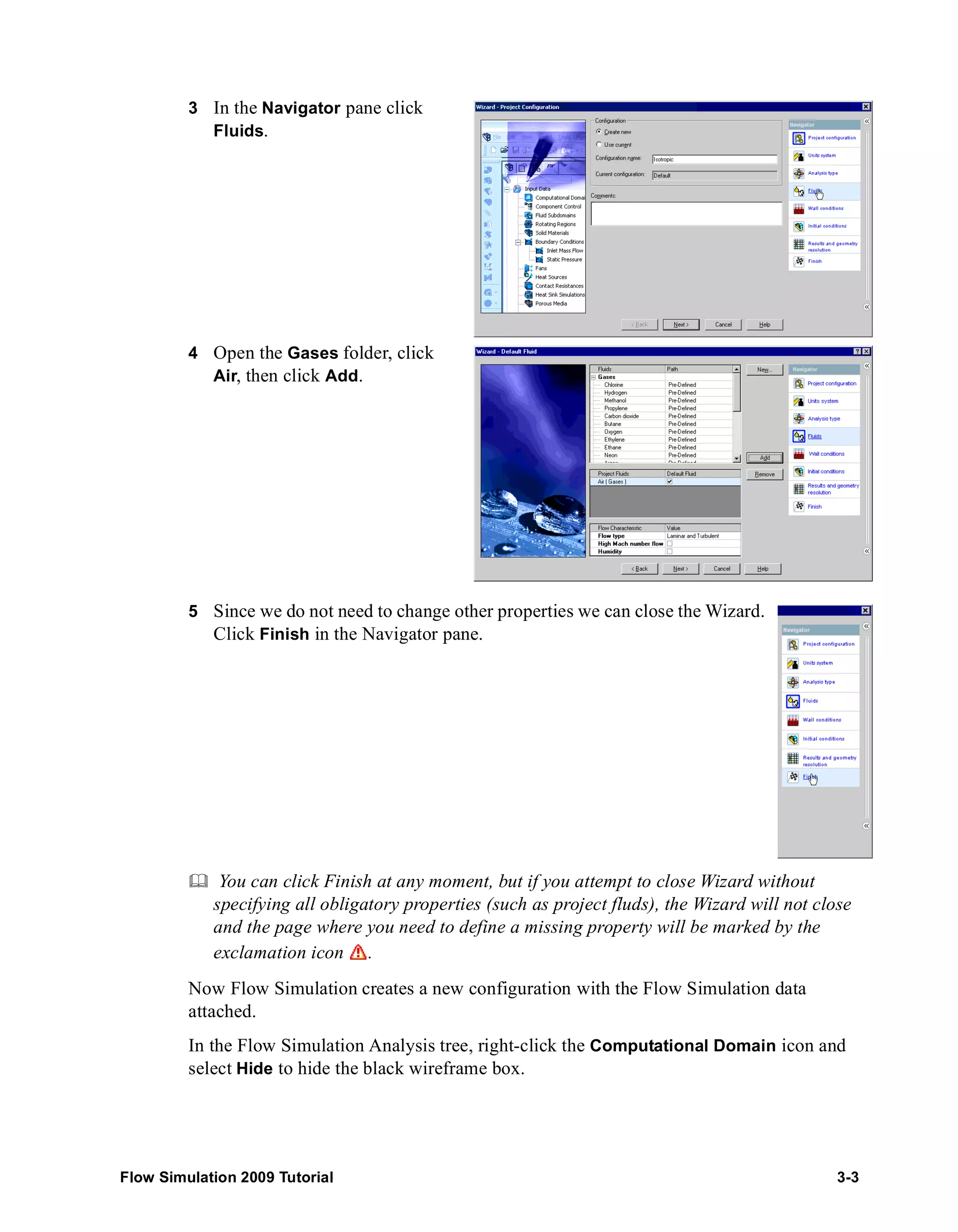
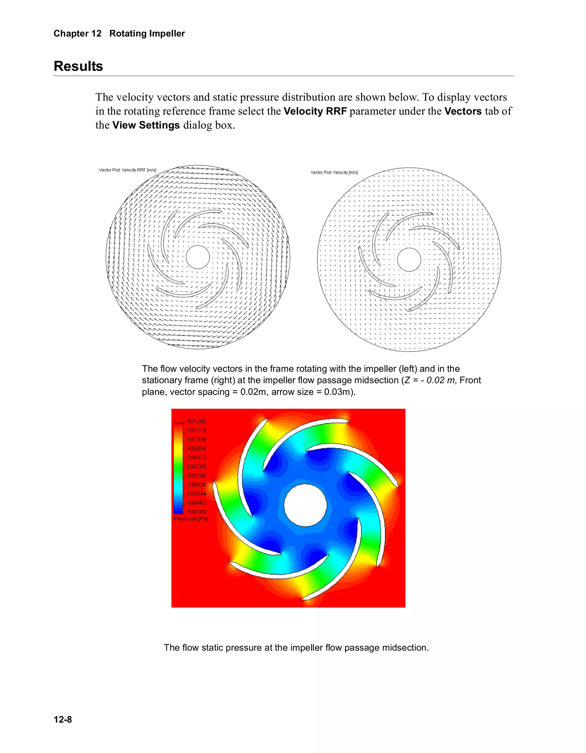
![Chapter 3 First Steps - Porous Media
3-16
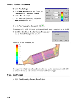
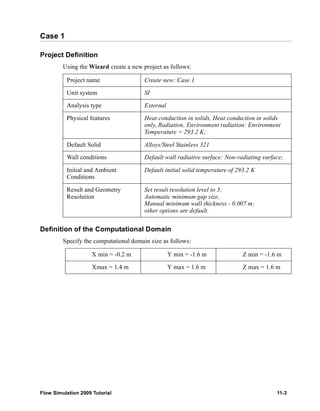
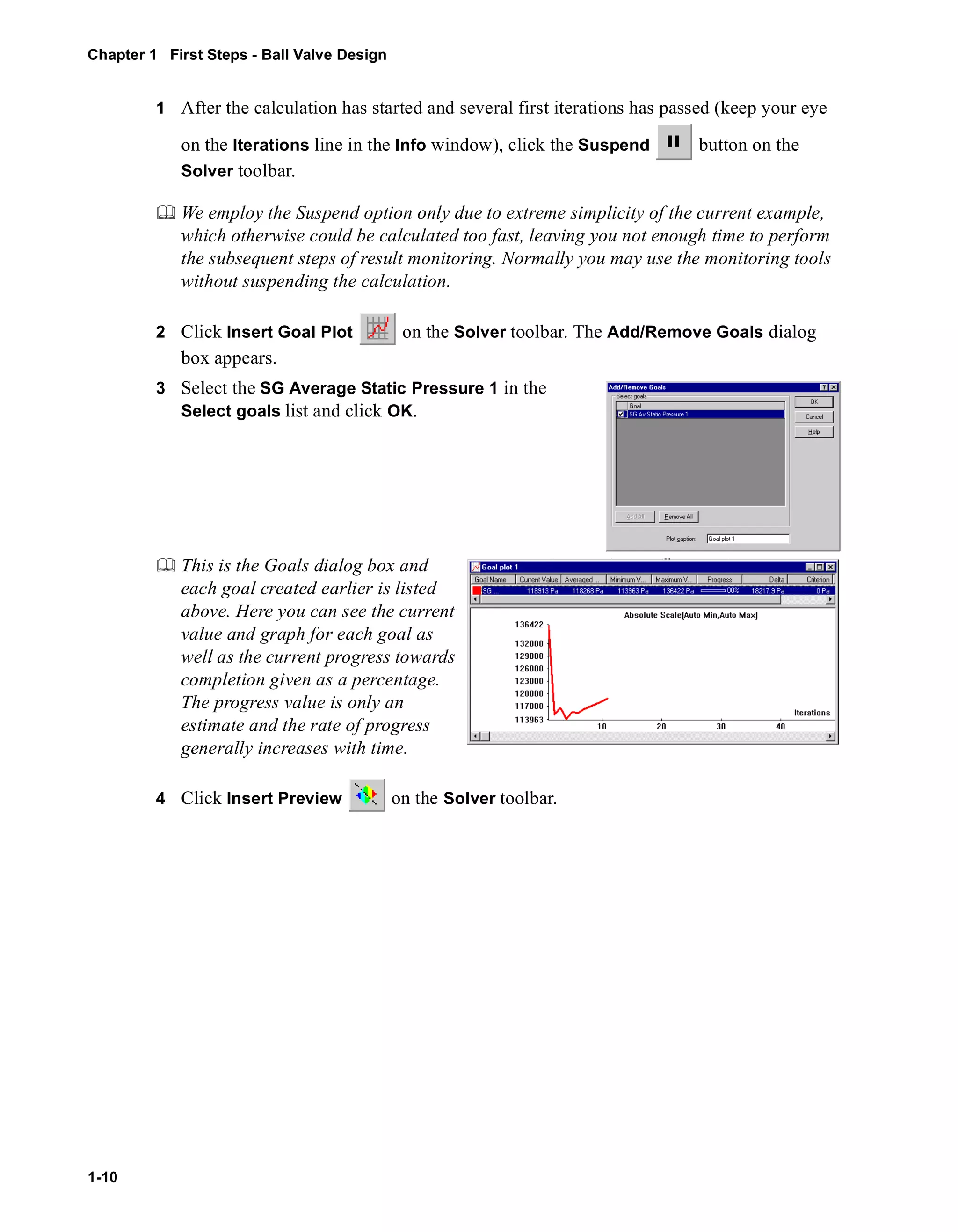
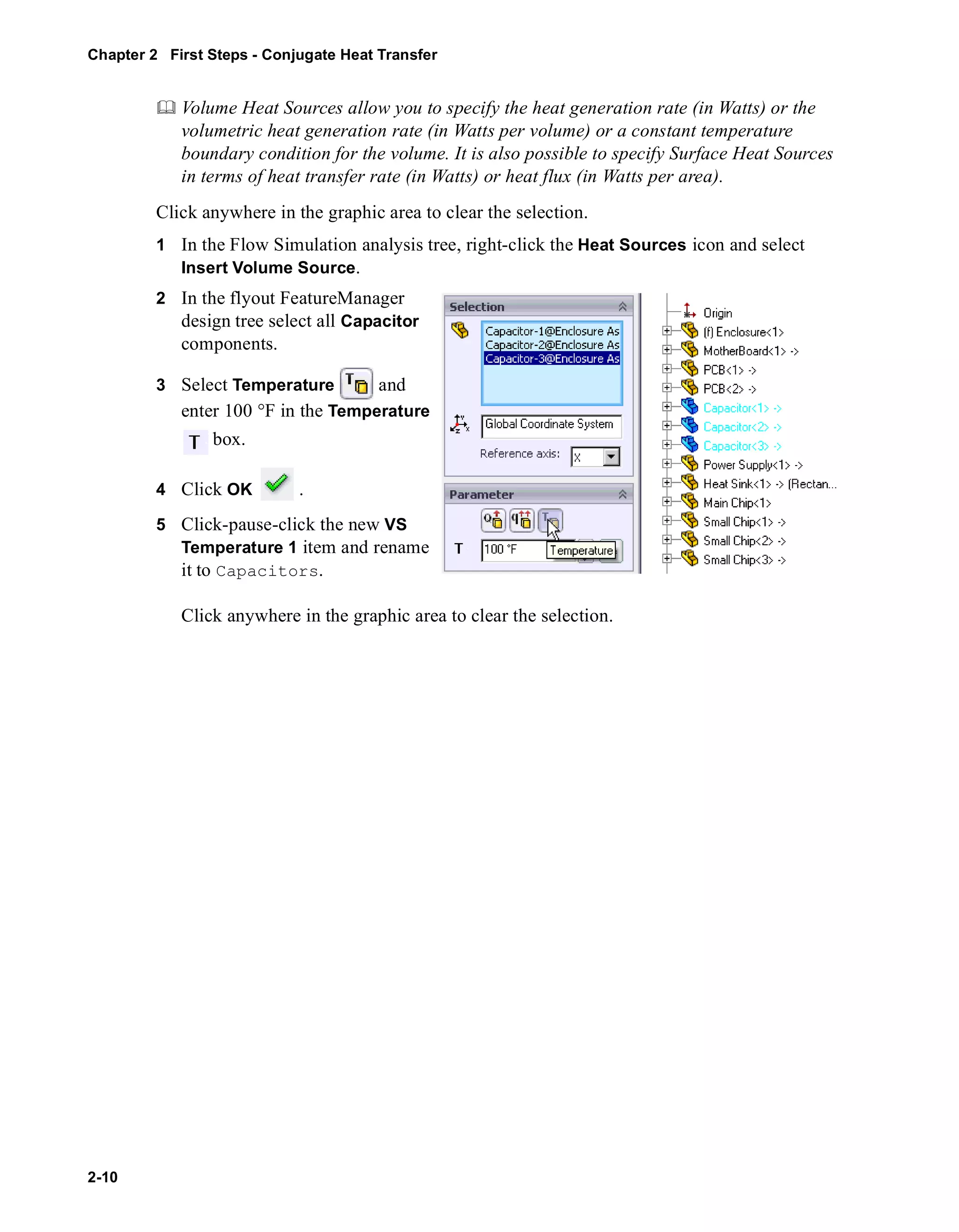
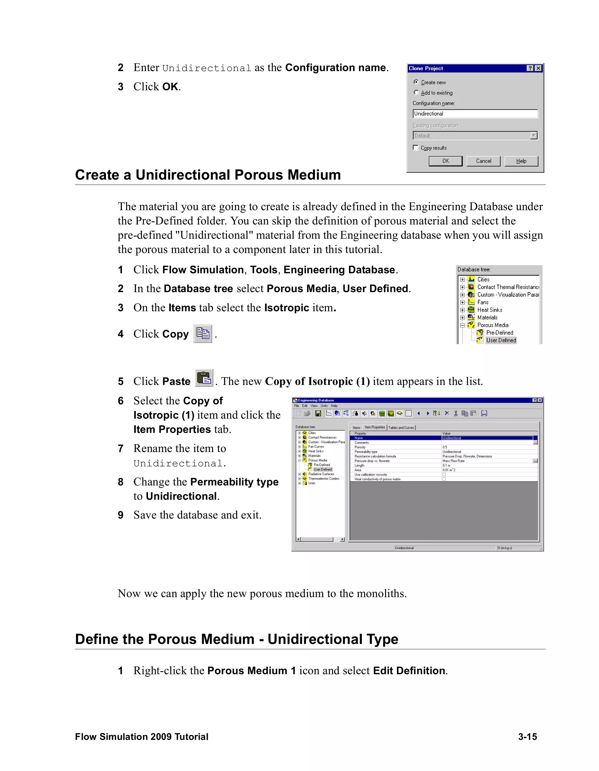
2 Expand the list of User Defined porous medium and
select Unidirectional. If you skipped the definition of the
unidirectional porous medium, use the Unidirectional
material available under Pre-Defined.
3 In the Direction select the Z axis of the Global
Coordinate System.
For porous media having unidirectional permeability, we
must specify the permeability direction as an axis of the
selected coordinate system (axis Z of the Global
coordinate system in our case).
4 Click OK .
Since all other conditions and goals remain the same, we can
start the calculation immediately
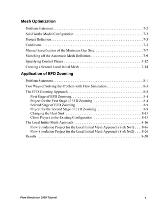
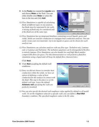
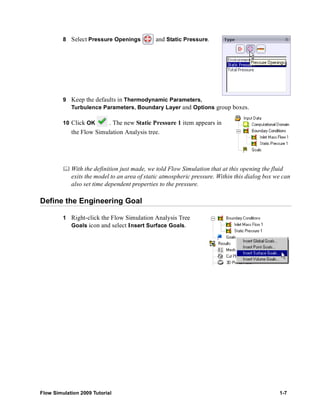
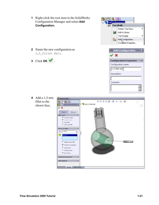
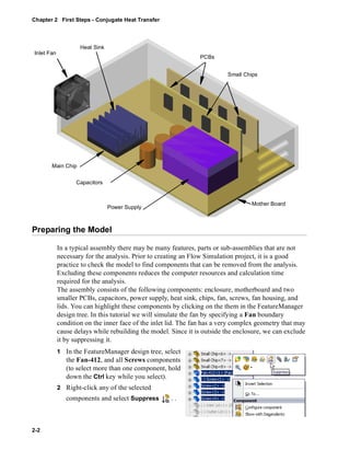
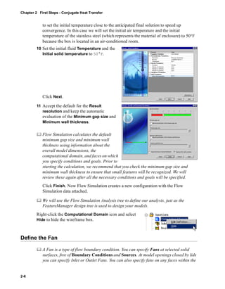
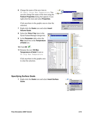
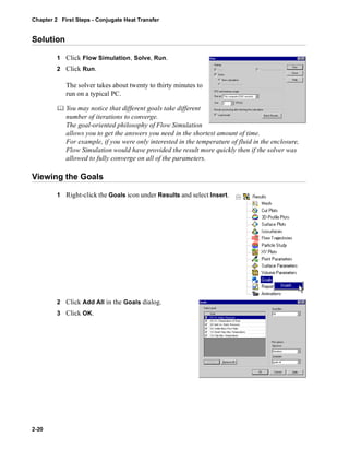
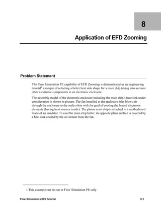
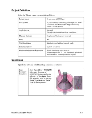
Compare the Isotropic and Unidirectional Catalysts
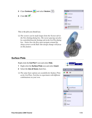
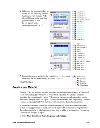
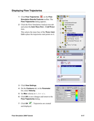
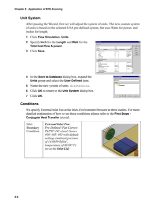
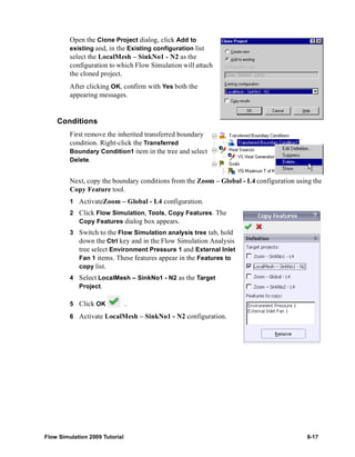
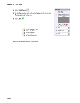
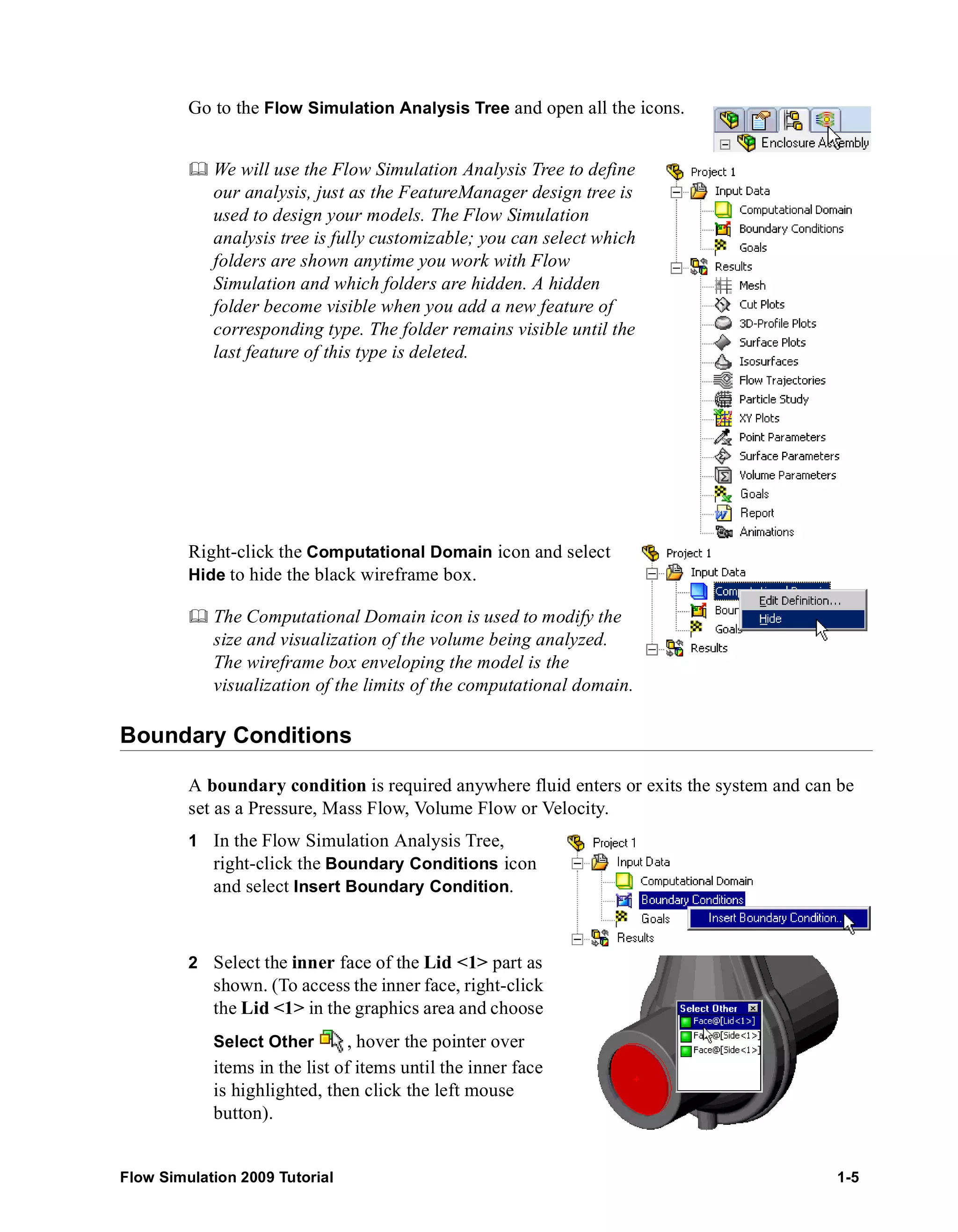
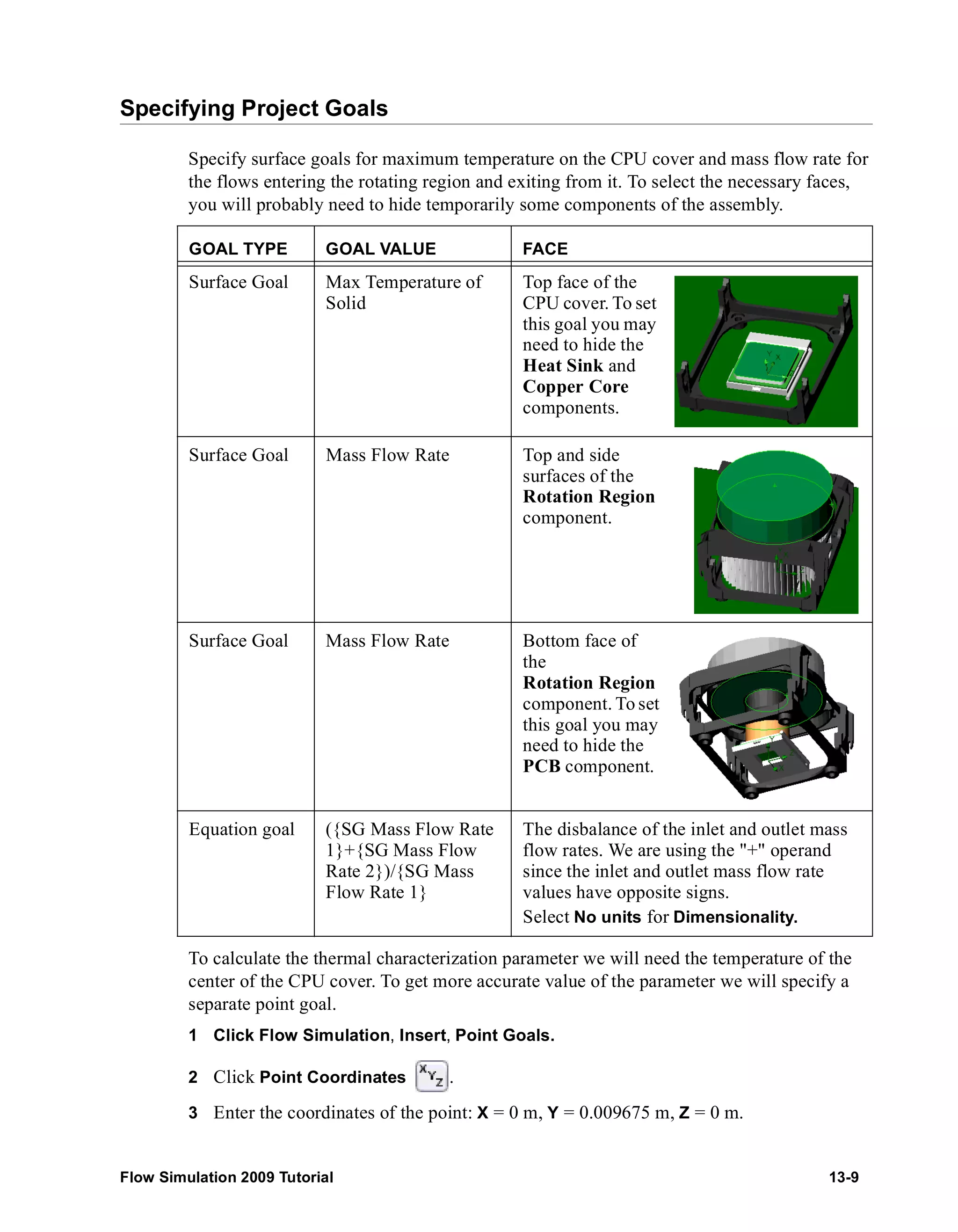
When the calculation is finished, create the goal plot for the Equation Goal 1.
Catalyst.SLDASM [Unidirectional]
Goal Name Unit Value Averaged Value Minimum Value Maximum Value Progress [%] Use In Convergence
Equation Goal 1 [Pa] 117.0848512 118.6235708 117.0761518 121.5639633 100 Yes
Display flow trajectories as described above.
Comparing the trajectories passing through the isotropic and unidirectional porous
catalysts installed in the tube, we can summarize:](https://image.slidesharecdn.com/swflowsimulation2009tutorial-141007202601-conversion-gate02/85/Sw-flowsimulation-2009-tutorial-90-320.jpg)


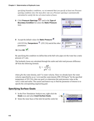


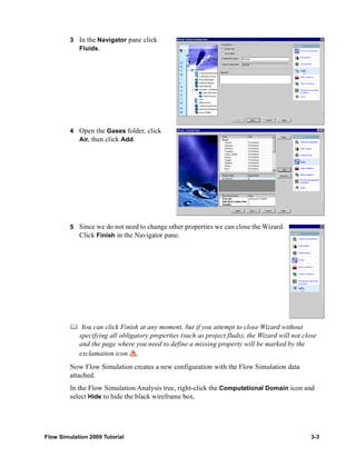
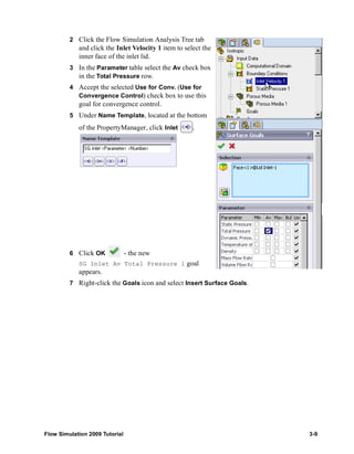
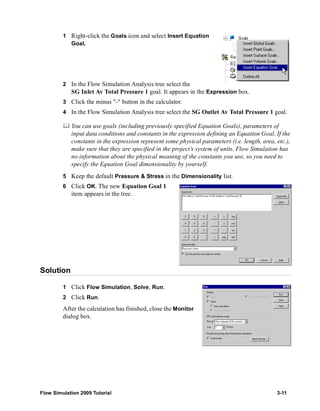
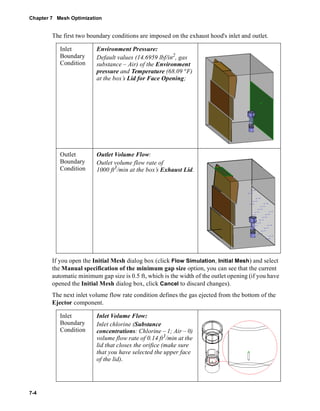
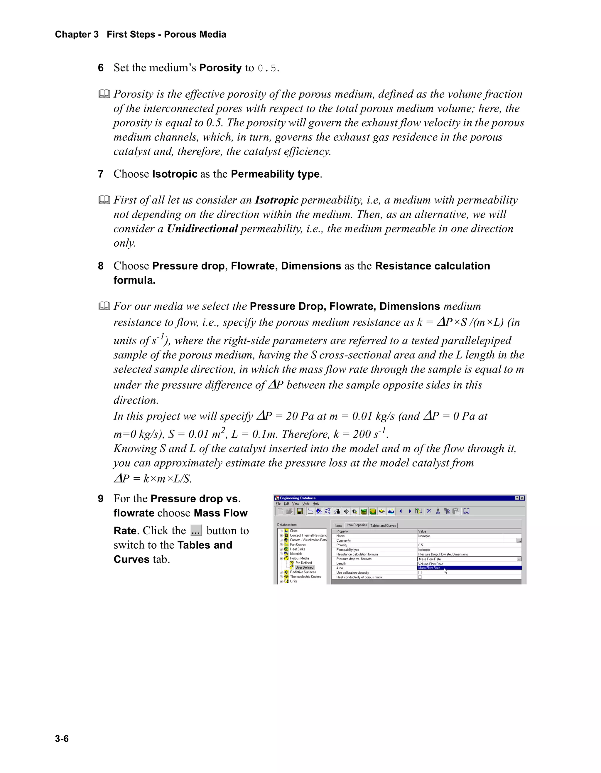
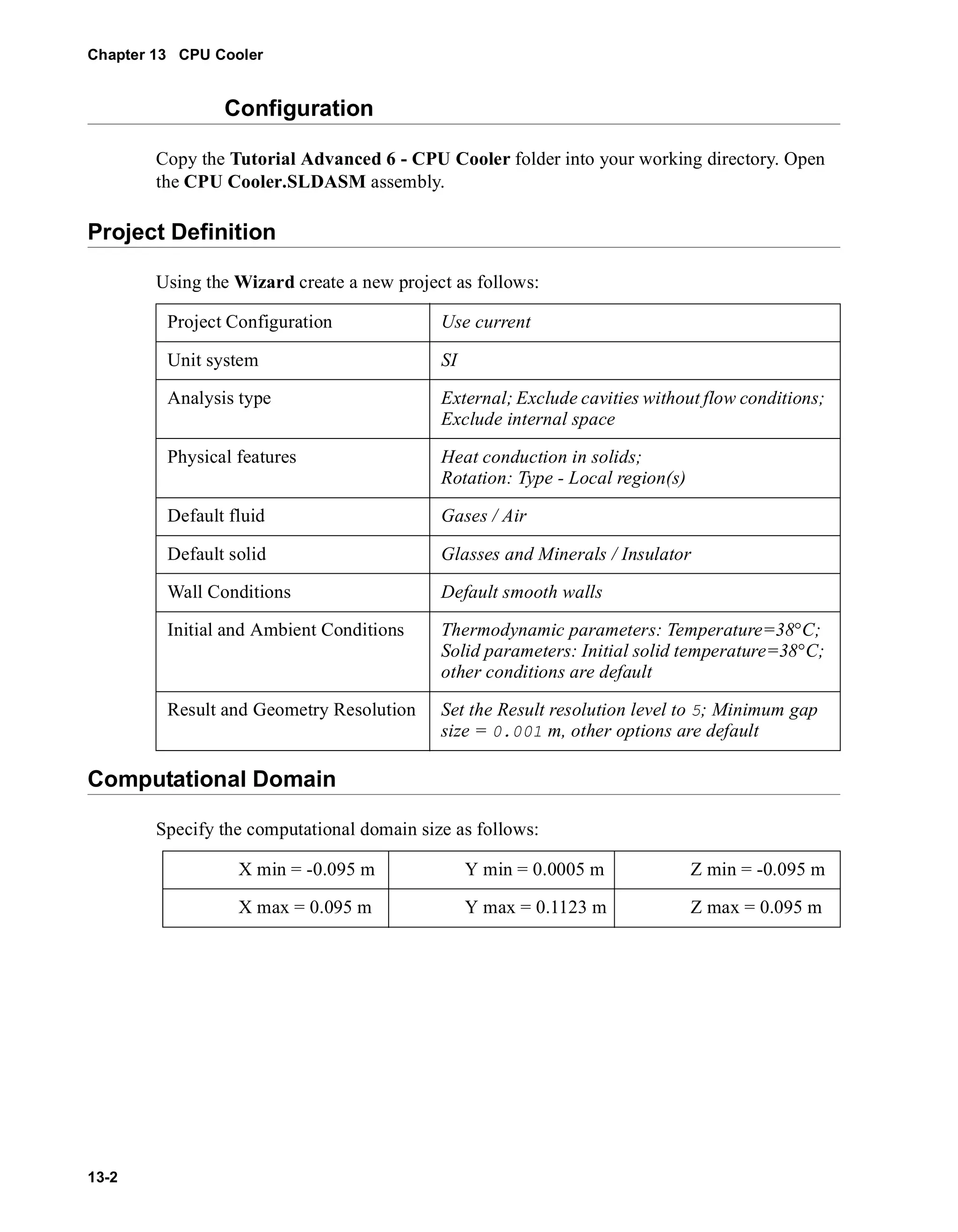
![Chapter 4 Determination of Hydraulic Loss
4-16
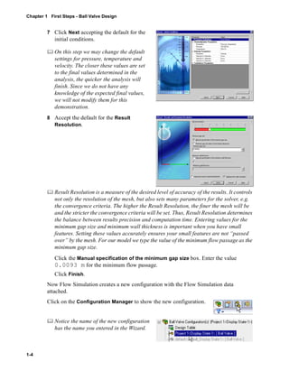
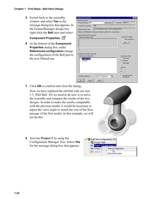
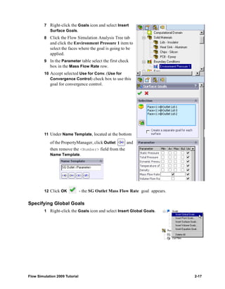
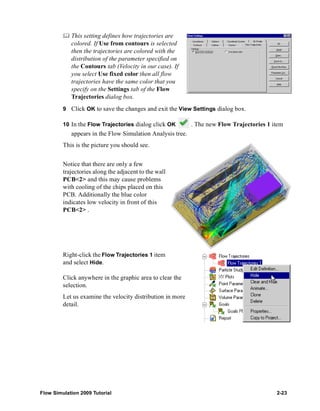
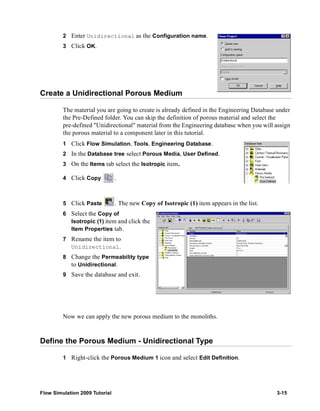
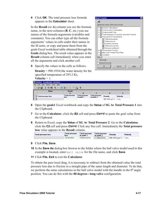
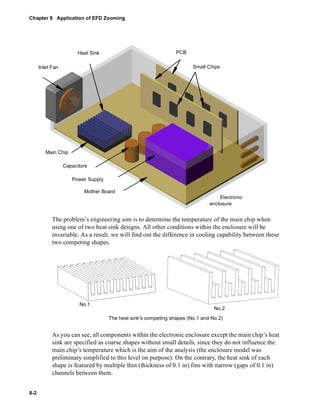
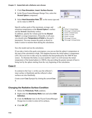
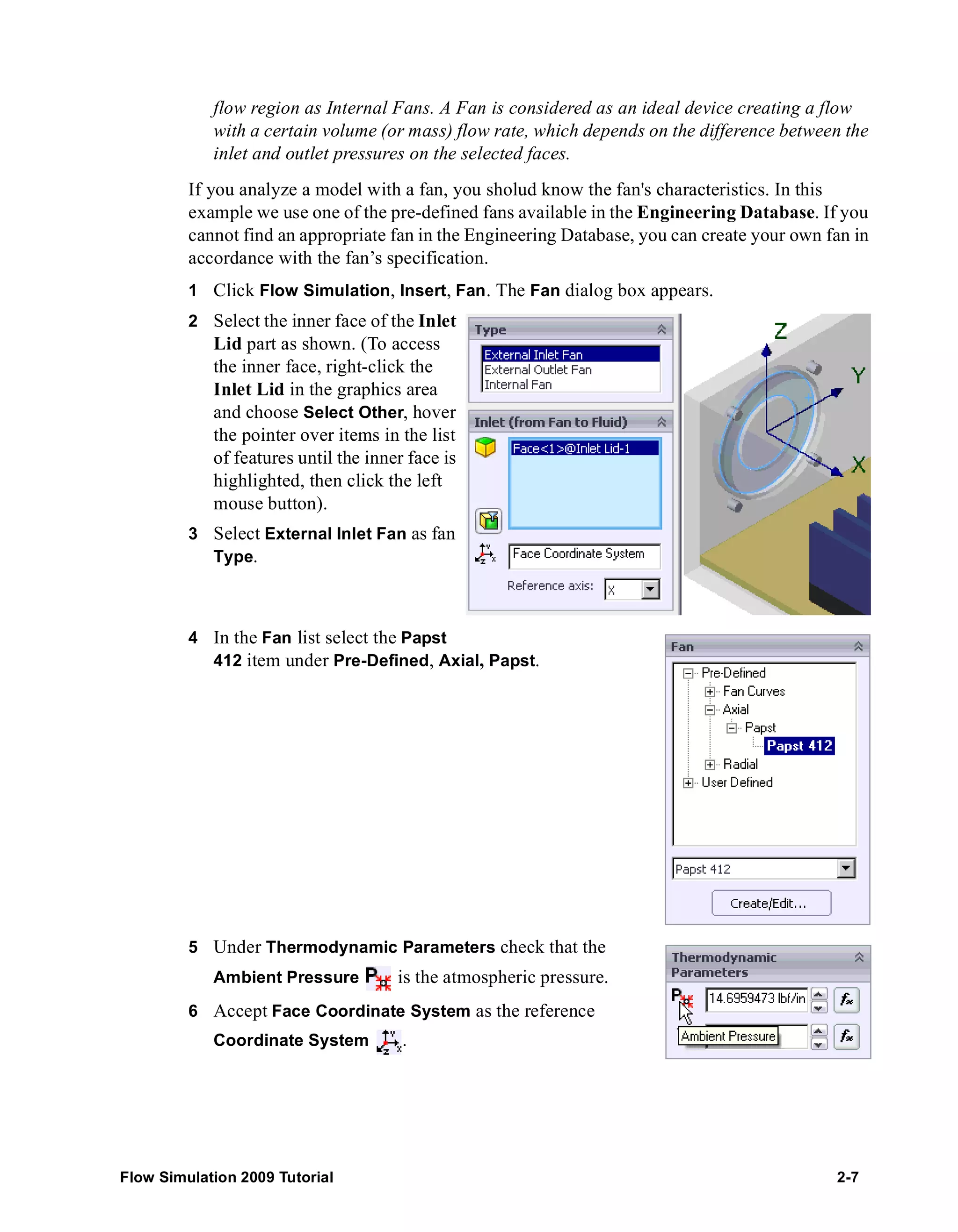
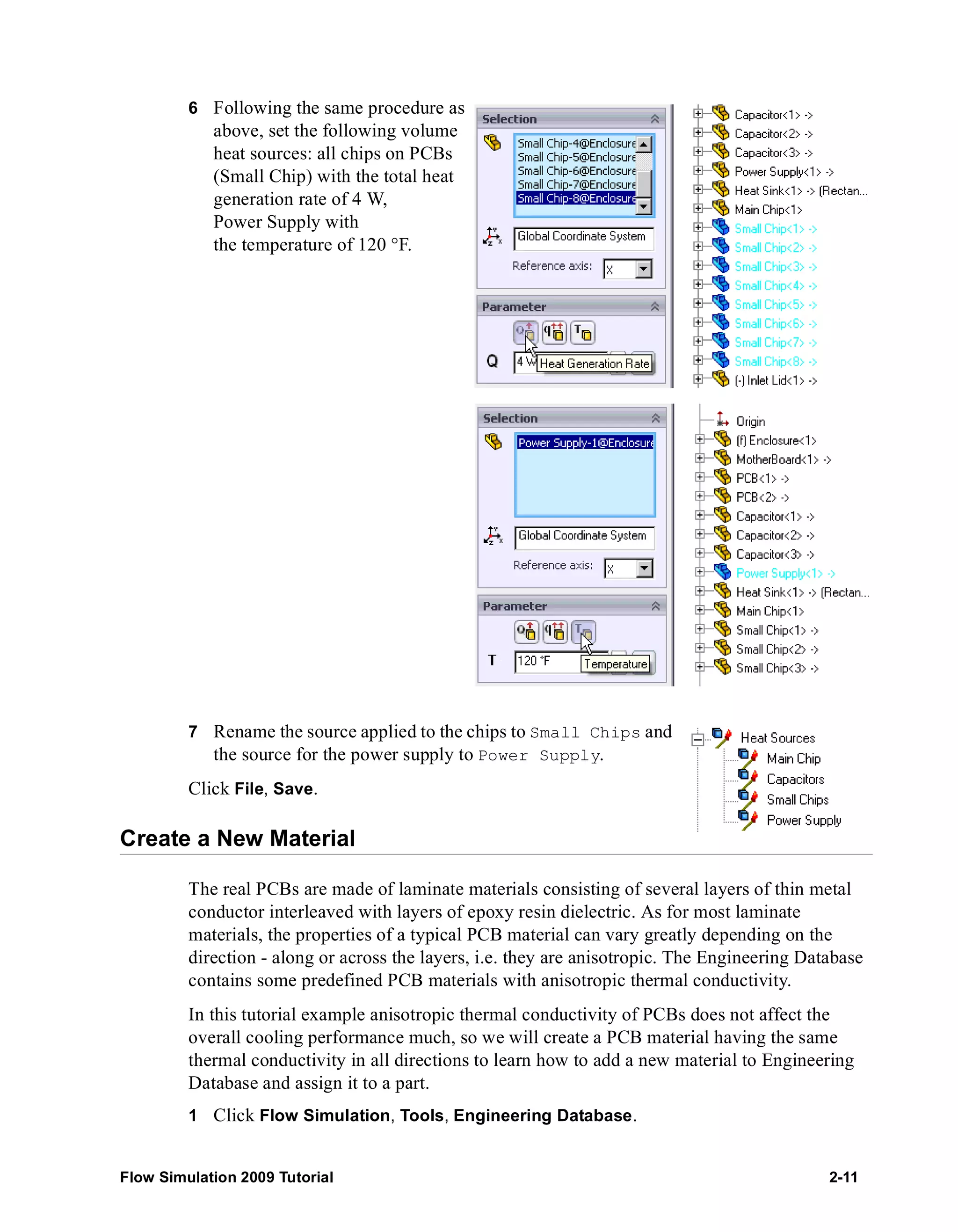
2 Click Add All.
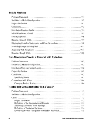
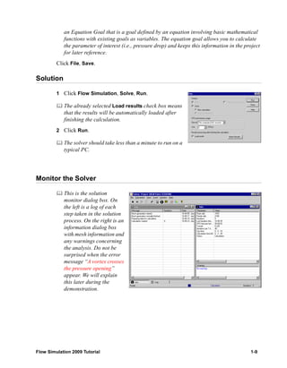
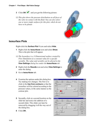
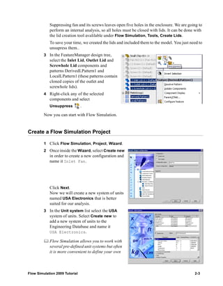
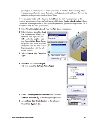
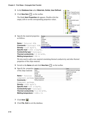
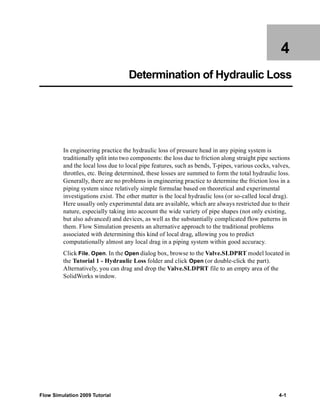
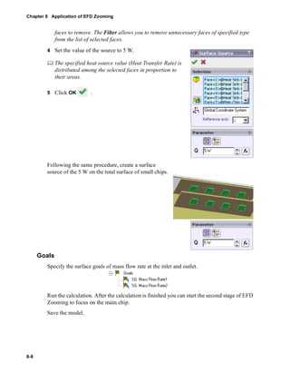
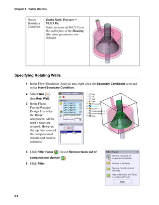
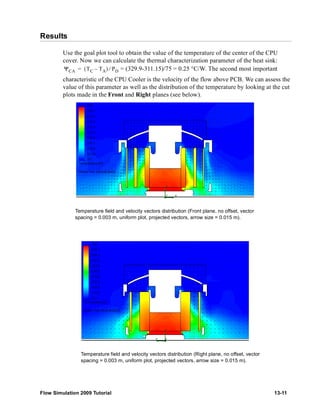
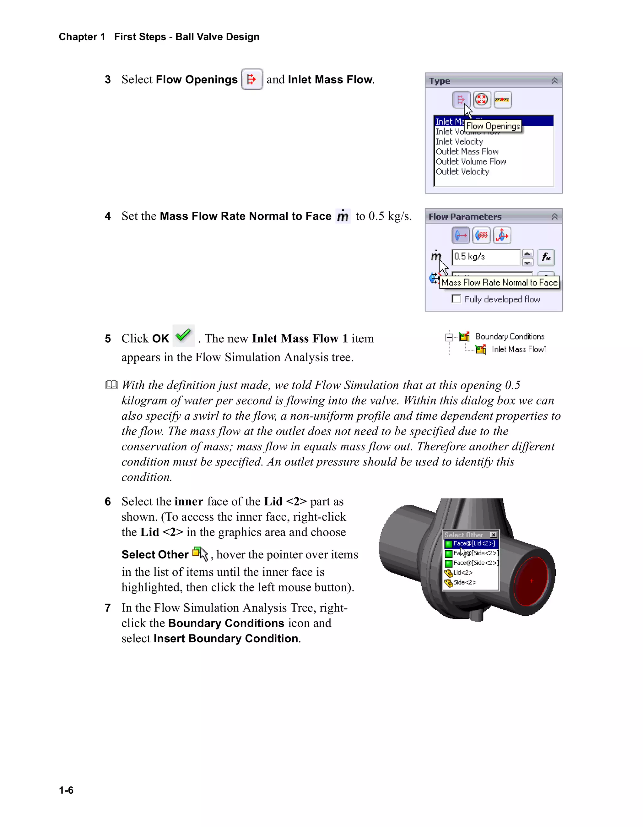
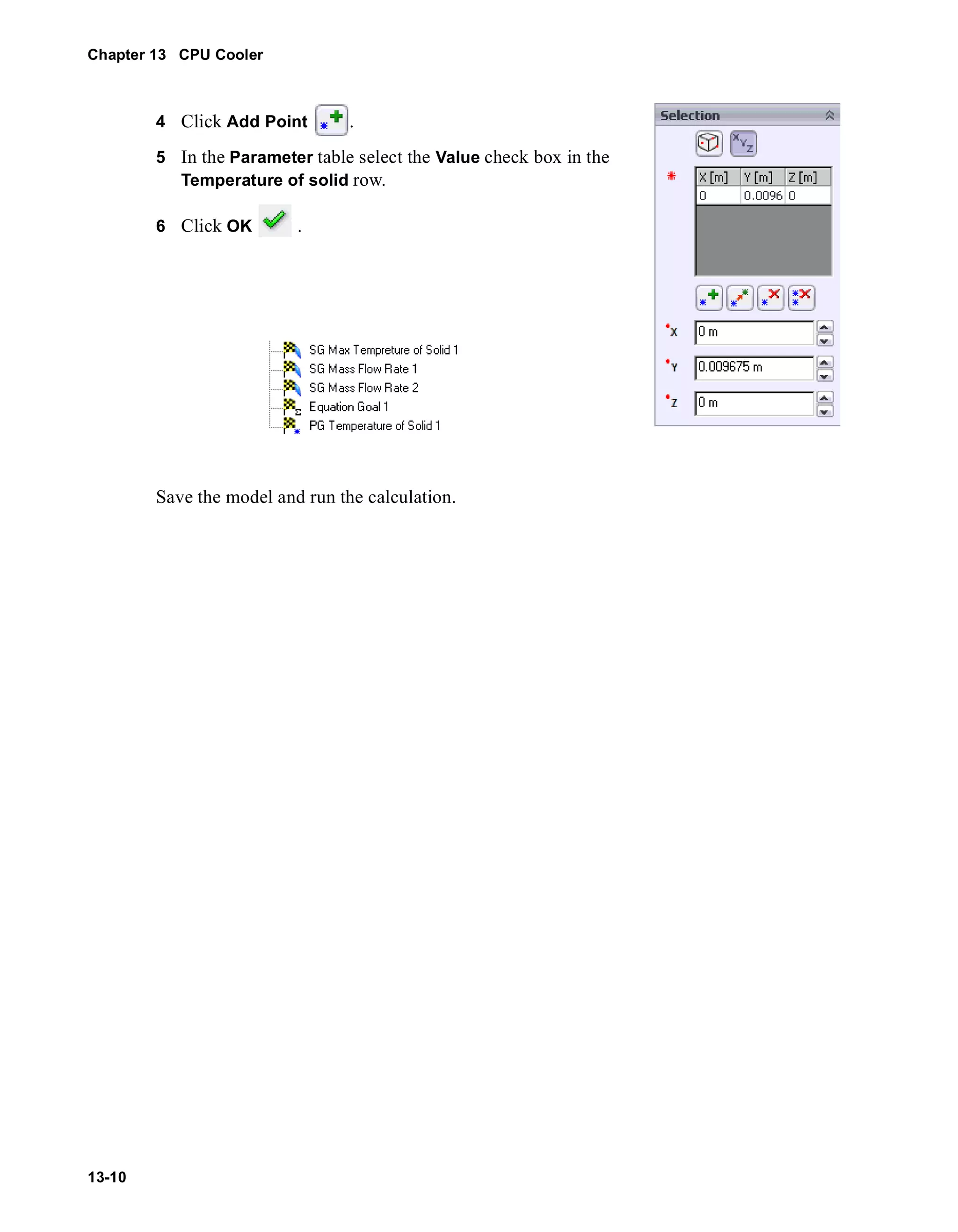
3 Click OK. The goals1 Excel workbook is
created.
This workbook displays how the goal changed
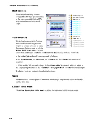
during the calculation. You can take the total
pressure value presented at the Summary sheet.
Valve.SLDPRT [40 degrees - long valve]
Goal Name Unit Value Averaged Value Minimum Value Maximum Value Progress [%] Use In Convergence
SG Av Total Pressure 1 [Pa] 101833.4184 101833.8984 101833.3951 101834.7911 100 Yes
SG Av Total Pressure 2 [Pa] 111386.6792 111389.5793 111384.8369 111399.0657 100 Yes
In fact, to obtain the pressure loss it would be easier to specify an Equation goal with the
difference between the inlet and outlet pressures as the equation goal’s expression.
However, to demonstrate the wide capabilities of Flow Simulation, we will calculate the
pressure loss with the Flow Simulation gasdynamic Calculator.
The Calculator contains various formulae from fluid dynamics which can be useful for
engineering calculations. The calculator is a very useful tool for rough estimations of
the expected results, as well as for calculations of important characteristic and
reference values. All calculations in the Calculator are performed only in the
International system of units SI, so no parameter units should be entered, and Flow
Simulation Units settings do not apply in the Calculator.
Working with Calculator
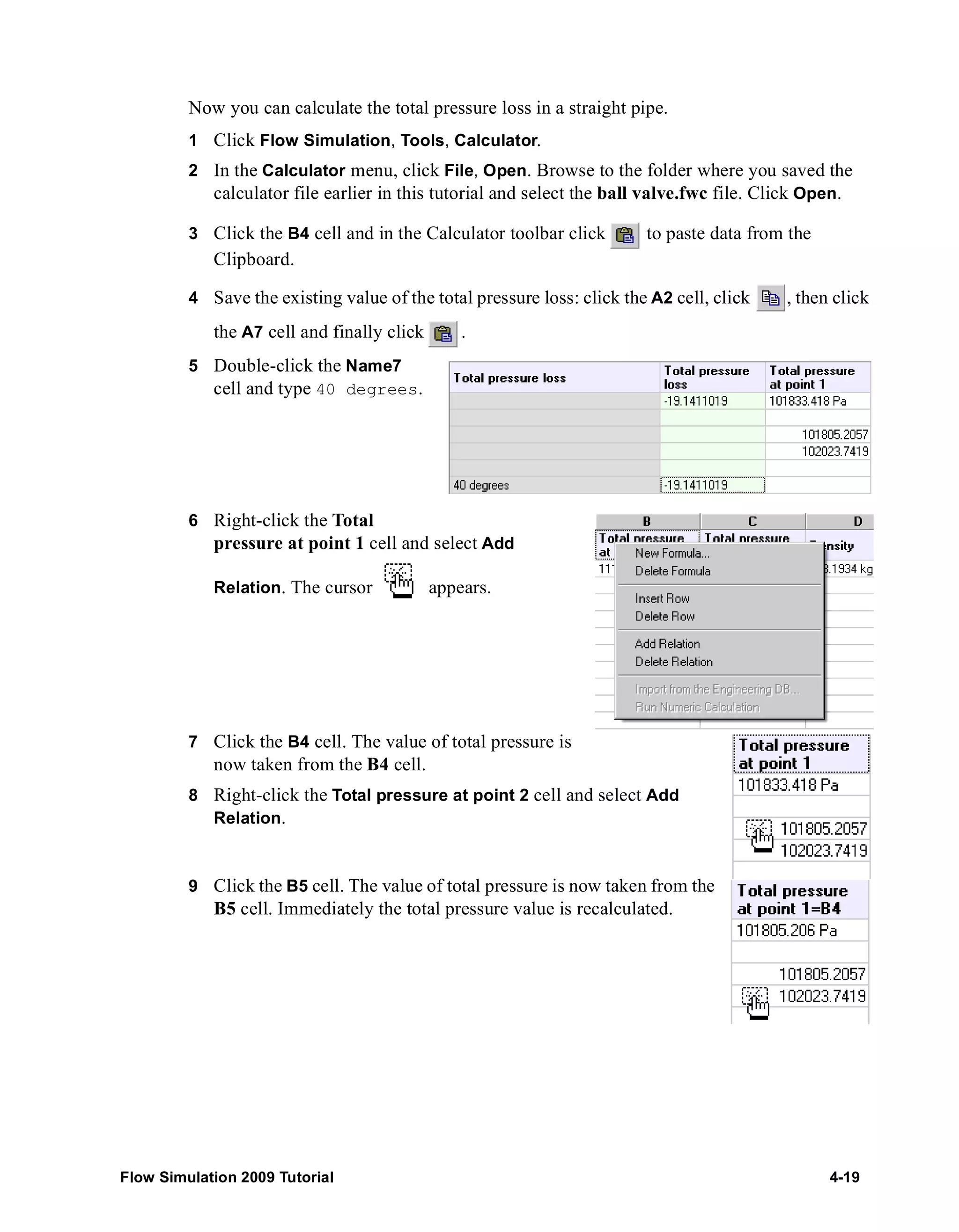
1 Click Flow Simulation, Tools, Calculator.
2 Right-click the A1 cell in the Calculator sheet
and select New Formula. The New Formula
dialog box appears.
3 In the Select the name of the new formula tree
expand the Pressure and Temperature item
and select the Total pressure loss check box.](https://image.slidesharecdn.com/swflowsimulation2009tutorial-141007202601-conversion-gate02/85/Sw-flowsimulation-2009-tutorial-108-320.jpg)
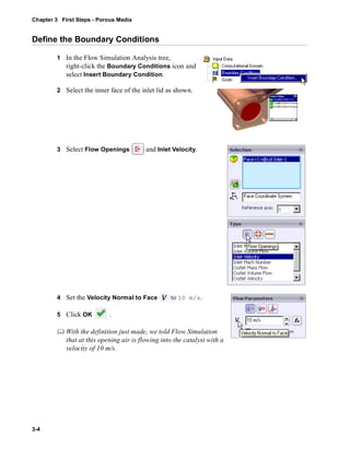
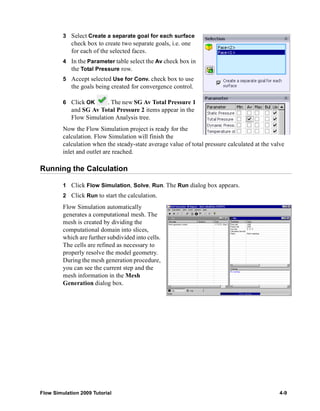
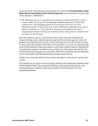
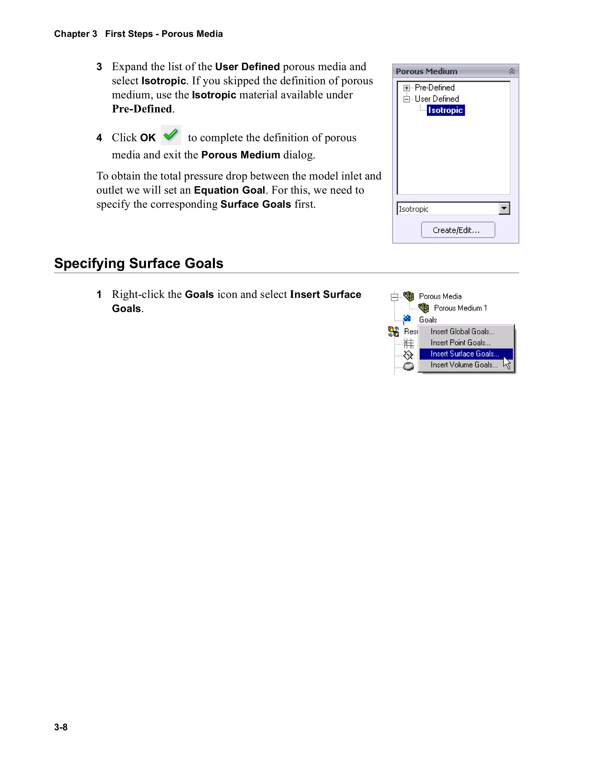
![Chapter 4 Determination of Hydraulic Loss
4-18
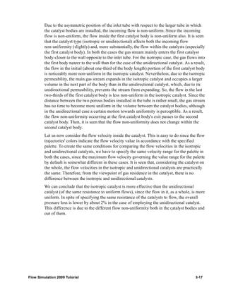
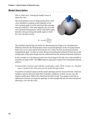
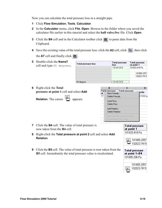
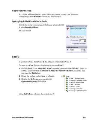
Since the specified conditions are the same for both 40 degrees - long valve and 00
degrees - long valve configurations, it is useful to attach the existing Flow Simulation
project to the 00 degrees - long valve configuration.
Clone the current project to the 00 degrees - long valve
configuration.
Since at zero angle the ball valve becomes a simple straight pipe, there is no need to set the
Minimum gap size value smaller than the default gap size which, in our case, is
automatically set equal to the pipe’s diameter (the automatic minimum gap size depends
on the characteristic size of the faces on which the boundary conditions are set). Note that
using a smaller gap size will result in a finer mesh and, in turn, more computer time and
memory will be required for calculation. To solve your task in the most effective way you
should choose the optimal settings for the task.
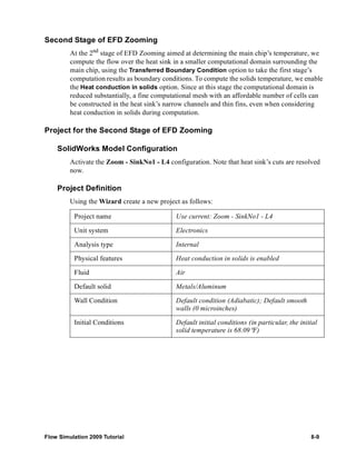
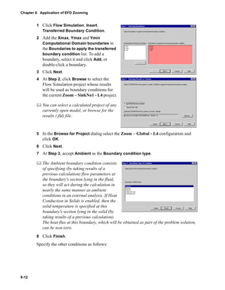
Changing the Geometry Resolution
Check to see that the 00 degrees - long valve is the active configuration.
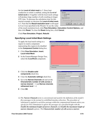
1 Click Flow Simulation, Initial Mesh.
2 Clear the Manual specification of
the minimum gap size check box.
3 Click OK.
Click Flow Simulation, Solve, Run.
Then click Run to start the calculation.
After the calculation is finished, create
the Goal Plot. The goals2 workbook is
created. Go to Excel, then select the both
cells in the Value column and copy them
into the Clipboard.
Goal Name Unit Value Averaged Value Minimum Value
SG Av Total Pressure 1 [Pa] 101805.2057 101804.8525 101801.4794
SG Av Total Pressure 2 [Pa] 102023.7419 102054.9498 102022.7459](https://image.slidesharecdn.com/swflowsimulation2009tutorial-141007202601-conversion-gate02/85/Sw-flowsimulation-2009-tutorial-110-320.jpg)
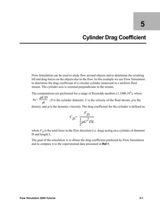


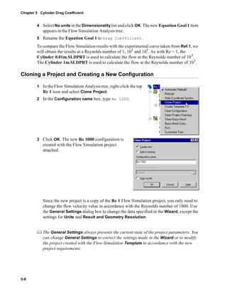
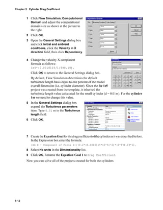
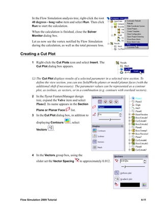
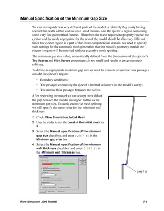
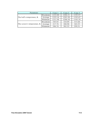
![Chapter 5 Cylinder Drag Coefficient
5-14
cylinder 0.01m.SLDPRT [Re 1000]
Goal Name Unit Value Averaged Value Minimum Value Maximum Value
GG X - Component of Force [N] 0.000104929 9.71368E-05 8.75382E-05 0.000105358
Drag Coefficient [ ] 1.023705931 0.94768731 0.85404169 1.027899399
6 Activate the Re 1 configuration and load results. Create the goal plot for both the goals.
cylinder 0.01m.SLDPRT [Re 1]
Goal Name Unit Value Averaged Value Minimum Value Maximum Value
GG X - Component of Force [N] 1.14448E-09 1.16764E-09 1.12756E-09 1.81674E-09
Drag Coefficient [ ] 11.16575499 11.39179479 11.00070462 17.72455528
7 Switch to the cylinder 1m part, activate the Re 1e5 configuration, load results and
create the goal plot for both the goals.
cylinder 1m .SLDPRT [Re 1e5]
Goal Name Unit Value Averaged Value Minimum Value Maximum Value
GG X - Component of Force [N] 0.482967811 0.478070888 0.465937059 0.491484755
Drag Coefficient [ ] 0.471193865 0.46641632 0.454578294 0.47950318
Even if the calculation is steady, the averaged value is more preferred, since in this case
the oscillation effect is of less perceptibility. We will use the averaged goal value for the
other two cases as well.
You can now compare Flow Simulation results with the experimental curve.
0.1 1 10 100 1000 10000 100000 100000
0
Re
1E+07
Ref. 1 Roland L. Panton, “Incompressible flow” Second edition. John Wiley & sons Inc., 1995](https://image.slidesharecdn.com/swflowsimulation2009tutorial-141007202601-conversion-gate02/85/Sw-flowsimulation-2009-tutorial-126-320.jpg)


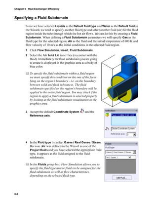
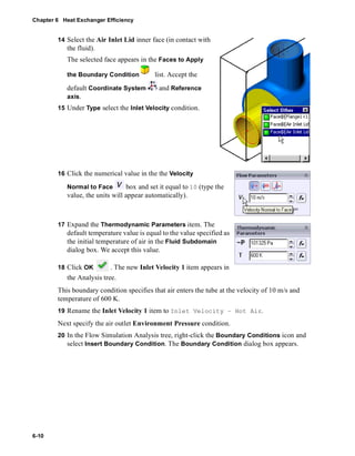
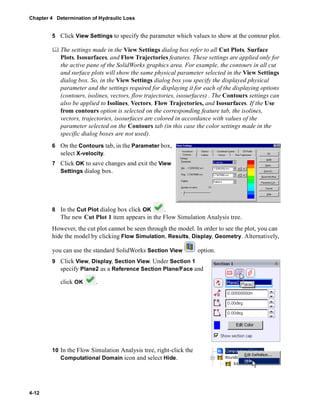
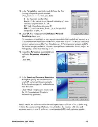
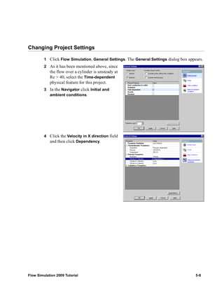
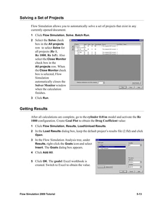
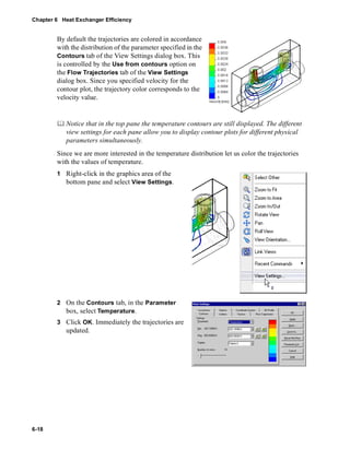
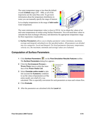
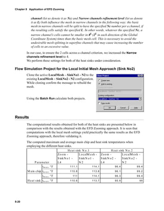
![Chapter 6 Heat Exchanger Efficiency
6-14
Click View, Toolbars, Flow Simulation Display. The
Flow Simulation Display toolbar appears.
The SolidWorks CommandManager is a dynamically-updated, context-sensitive toolbar,
which allows you to save space for the graphics area and access all toolbar buttons from
one location. The tabs below the CommandManager is used to select a specific group of
commands and features to make their toolbar buttons available in the CommandManager.
To get access to the Flow Simulation commands and features, click the Flow Simulation
tab of the CommandManager.
If you wish, you may hide the Flow Simulation toolbars to save the space for the graphics
area, since all necessary commands are available in the CommandManager. To hide a
toolbar, click its name again in the View, Toolbars menu.
1 Click Goals on the Results Main toolbar or CommandManager. The Goals dialog
box appears.
2 Click Add All to select all goals of the project
(actually, in our case there is only one goal) .
3 Click OK. The goals1 Excel workbook is
created.
You can view the average temperature of the tube on the Summary sheet.
Heat Exchanger.SLDASM [Level 3]
Goa l Name Unit Value Ave raged Va lue Minimum Va lue Ma x imum V alue Progre ss [%] Use In Convergence
VG Av T of Tube [K] 328.4682387 327.4703038 324.7176733 328.4682387 100 Yes
Iterations: 51
Analysis in terval: 21
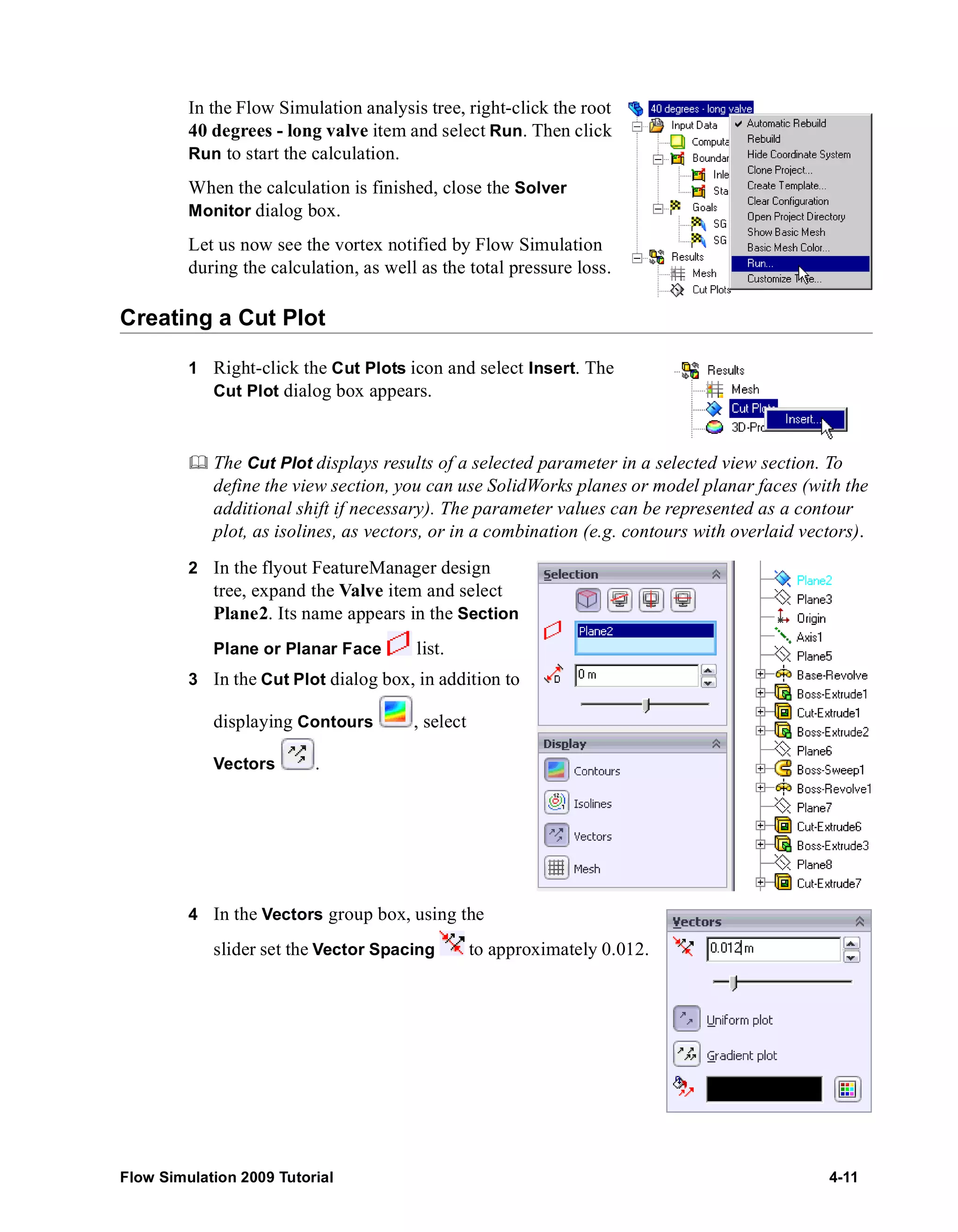
Creating a Cut Plot
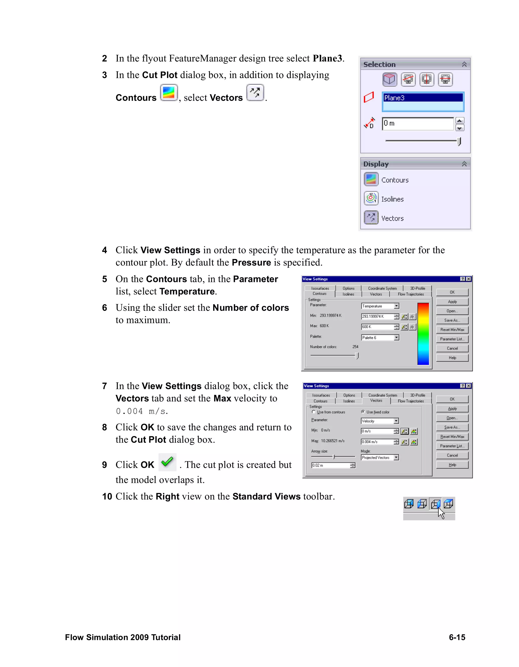
1 Click Cut Plot on the Flow Simulation Results Features toolbar. The Cut Plot
dialog box appears.](https://image.slidesharecdn.com/swflowsimulation2009tutorial-141007202601-conversion-gate02/85/Sw-flowsimulation-2009-tutorial-140-320.jpg)
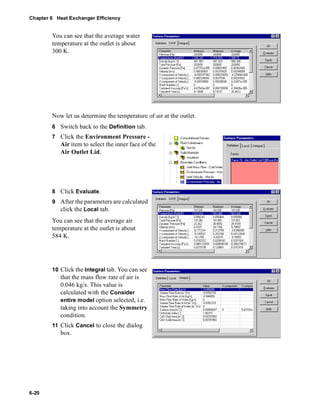


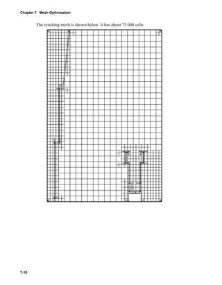


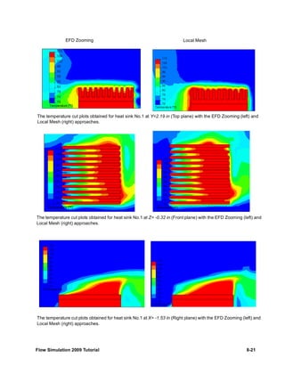

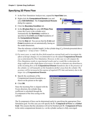
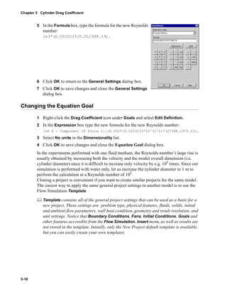
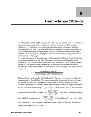
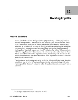
![Chapter 10 Non-Newtonian Flow in a Channel with Cylinders
10-4
Run the calculation. When the calculation is finished, create the goal plot to obtain the
pressure drop between the channel’s inlet and outlet.
Array o f C ylinders.SLDPRT [XGS]
Go a l Nam e Unit Va lue Ave ra ge d Va lue Minim um V a lue Ma x im um V a lue Progre ss [%]
SG A v Total P res sure 1 [P a] 105622.4926 105622.4125 105620.3901 105627.4631 100
SG A v Total P res sure 2 [P a] 101329.0109 101329.0091 101329.0051 101329.0109 100
Pres sure Drop [P a] 4293.481659 4293.4034 4298.457377 4291.380166 100
It is seen that the channel's total pressure loss is about 4 kPa.
Comparison with Water
Let us now consider the flow of water in the same channel under the same conditions (at
the same volume flow rate).
Create a new configuration by cloning the current
project, and name it Water.
Changing Project Settings
1 Click Flow Simulation, General
Settings.
2 On the Navigator click Fluids.
3 In the Project Fluids table, select
XGum and click Remove. Answer
OK to the appearing warning
message.
4 Select Water in Liquids and click
Add.
5 Under Flow Characteristics, change
Flow type to Laminar and Turbulent.
6 Click OK.
Run the calculation. After the calculation is finished, create the goal plot.](https://image.slidesharecdn.com/swflowsimulation2009tutorial-141007202601-conversion-gate02/85/Sw-flowsimulation-2009-tutorial-206-320.jpg)
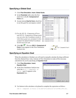
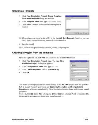
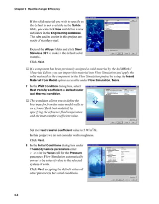
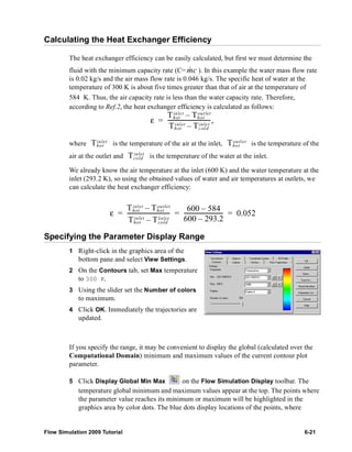
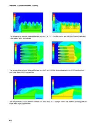
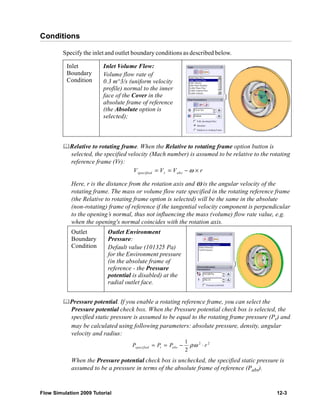
![Array o f C ylinders.SLDPRT [water]
Go a l Nam e Unit Va lue Ave ra ge d Va lue Minim um V a lue Ma x im um V a lue Progre ss [%]
SG A v Total P res sure 1 [P a] 101395.004 101395.0214 101394.8731 101395.1171 100
SG A v Total P res sure 2 [P a] 101329.3912 101329.3378 101329.3084 101329.3912 100
Pres sure Drop [P a] 65.6128767 65.68357061 65.76566097 65.55243288 100
As shown in the results table above, the channel's total pressure loss is about 60 Pa, i.e.
60...70 times lower than with the 3% aqueous solution of xanthan gum, this is due to the
water's much smaller viscosity under the problem's flow shear rates.
The XGS (above) and water velocity distribution in the range from 0 to 30 cm/s.
1 Georgiou G., Momani S., Crochet M.J., and Walters K. Newtonian and Non-Newtonian
Flow in a Channel Obstructed by an Antisymmetric Array of Cylinders. Journal of
Non-Newtonian Fluid Mechanics, v.40 (1991), p.p. 231-260.
Flow Simulation 2009 Tutorial 10-5](https://image.slidesharecdn.com/swflowsimulation2009tutorial-141007202601-conversion-gate02/85/Sw-flowsimulation-2009-tutorial-207-320.jpg)


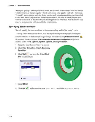
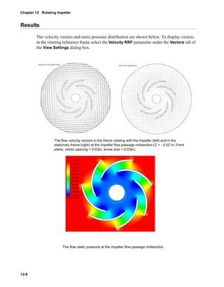
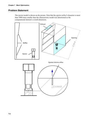
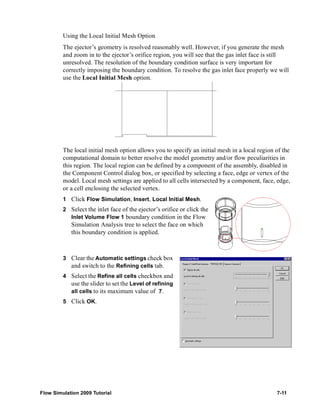
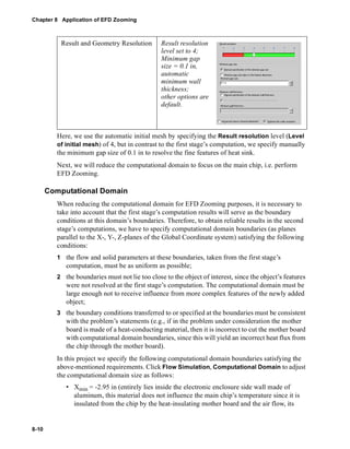
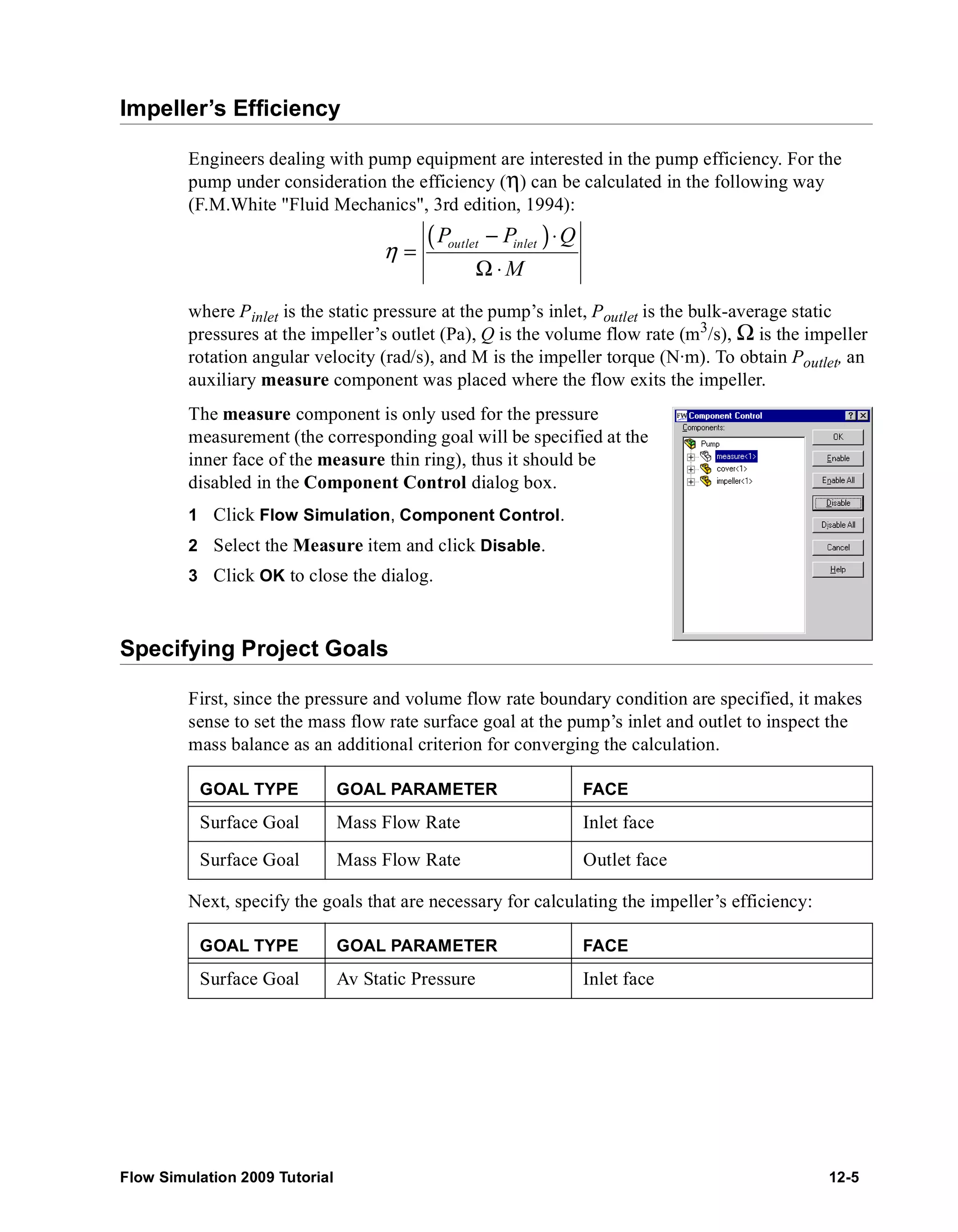
![The flow pressure distribution
For the impeller under consideration the obtained efficiency is 0.79.
Goal Name Unit Value Averaged Value Minimum Value Maximum Value
Efficiency [ ] 0.787039615 0.786371 0.784334 0.787117
Flow Simulation 2009 Tutorial 12-9](https://image.slidesharecdn.com/swflowsimulation2009tutorial-141007202601-conversion-gate02/85/Sw-flowsimulation-2009-tutorial-227-320.jpg)


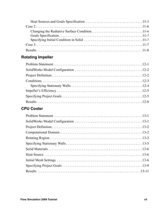
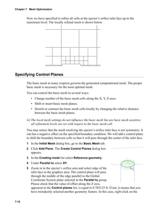
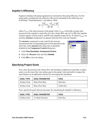
![An Excel spreadsheet with the goal results will open. The first sheet will show a table
summarizing the goals.
Enclosure Assembly.SLDASM [Inlet Fan (original)]
Goal Name Unit Value Averaged Value Minimum Value Maximum Value Progress [%] Use In Convergence
GG Av Static Pressure [lbf/in^2] 14.69678696 14.69678549 14.69678314 14.69678772 100 Yes
SG Inlet Av Static Pressure [lbf/in^2] 14.69641185 14.69641047 14.69640709 14.69641418 100 Yes
GG Av Temperature of Fluid [°F] 61.7814683 61.76016724 61.5252449 61.86764155 100 Yes
SG Outlet Mass Flow Rate [lb/s] -0.007306292 -0.007306111 -0.007306913 -0.007303663 100 Yes
VG Small Chips Max Temp [°F] 91.5523903 90.97688632 90.09851988 91.5523903 100 Yes
VG Chip Max Temperature [°F] 88.51909612 88.43365626 88.29145322 88.57515562 100 Yes
You can see that the maximum temperature in the main chip is about 88 °F, and the
maximum temperature over the small chips is about 91 °F.
Goal progress bar is a qualitative and quantitative characteristic of the goal
convergence process. When Flow Simulation analyzes the goal convergence, it
calculates the goal dispersion defined as the difference between the maximum and
minimum goal values over the analysis interval reckoned from the last iteration and
compares this dispersion with the goal's convergence criterion dispersion, either
specified by you or automatically determined by Flow Simulation as a fraction of the
goal's physical parameter dispersion over the computational domain. The percentage
of the goal's convergence criterion dispersion to the goal's real dispersion over the
analysis interval is shown in the goal's convergence progress bar (when the goal's real
dispersion becomes equal or smaller than the goal's convergence criterion dispersion,
the progress bar is replaced by word "Achieved"). Naturally, if the goal's real
dispersion oscillates, the progress bar oscillates also, moreover, when a hard problem
is solved, it can noticeably regress, in particular from the "achieved" level. The
calculation can finish if the iterations (in travels) required for finishing the calculation
have been performed, or if the goal convergence criteria are satisfied before
performing the required number of iterations. You can specify other finishing
conditions at your discretion.
To analyze the results in more detail let us use the various Flow Simulation
post-processing tools. The best method for the visualization of how the fluid flows inside
the enclosure is to create flow trajectories.
Flow Simulation 2009 Tutorial 2-21](https://image.slidesharecdn.com/swflowsimulation2009tutorial-141007202601-conversion-gate02/75/Sw-flowsimulation-2009-tutorial-65-2048.jpg)


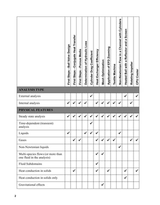
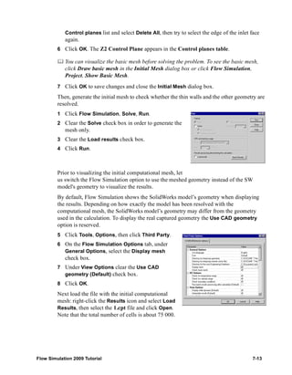
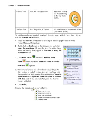
![Chapter 3 First Steps - Porous Media
Viewing the Goals
3-12
1 Right-click the Goals icon under Results and select Insert.
2 Select the Equation Goal 1 in the Goals
dialog box.
3 Click OK.
An Excel spreadsheet with the goal results will
open. The first sheet will contain a table
presenting the final values of the goal.
You can see that the total pressure drop is about 120 Pa.
Catalyst.SLDASM [Isotropic]
Goal Name Unit Value Averaged Value Minimum Value Maximum Value Progress [%] Use In Convergence
Equation Goal 1 [Pa] 120.0326909 121.774802 120.0326909 124.432896 100 Yes
To see the non-uniformity of the mass flow rate distribution over a catalyst’s cross section,
we will display flow trajectories with start points distributed uniformly across the inlet.](https://image.slidesharecdn.com/swflowsimulation2009tutorial-141007202601-conversion-gate02/75/Sw-flowsimulation-2009-tutorial-86-2048.jpg)


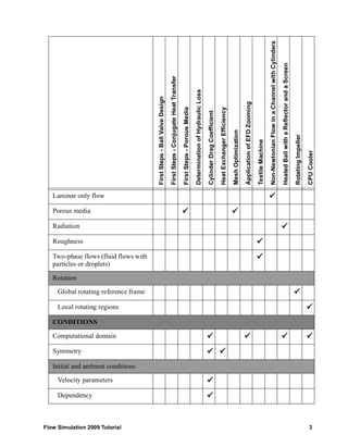
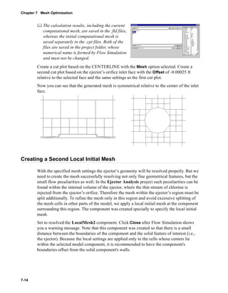
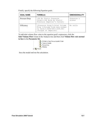
![Chapter 3 First Steps - Porous Media
3-16
2 Expand the list of User Defined porous medium and
select Unidirectional. If you skipped the definition of the
unidirectional porous medium, use the Unidirectional
material available under Pre-Defined.
3 In the Direction select the Z axis of the Global
Coordinate System.
For porous media having unidirectional permeability, we
must specify the permeability direction as an axis of the
selected coordinate system (axis Z of the Global
coordinate system in our case).
4 Click OK .
Since all other conditions and goals remain the same, we can
start the calculation immediately
Compare the Isotropic and Unidirectional Catalysts
When the calculation is finished, create the goal plot for the Equation Goal 1.
Catalyst.SLDASM [Unidirectional]
Goal Name Unit Value Averaged Value Minimum Value Maximum Value Progress [%] Use In Convergence
Equation Goal 1 [Pa] 117.0848512 118.6235708 117.0761518 121.5639633 100 Yes
Display flow trajectories as described above.
Comparing the trajectories passing through the isotropic and unidirectional porous
catalysts installed in the tube, we can summarize:](https://image.slidesharecdn.com/swflowsimulation2009tutorial-141007202601-conversion-gate02/75/Sw-flowsimulation-2009-tutorial-90-2048.jpg)


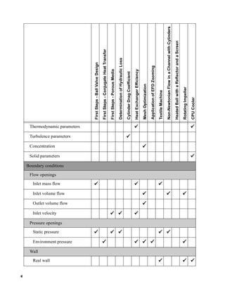
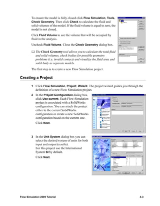
![Chapter 4 Determination of Hydraulic Loss
4-16
2 Click Add All.
3 Click OK. The goals1 Excel workbook is
created.
This workbook displays how the goal changed
during the calculation. You can take the total
pressure value presented at the Summary sheet.
Valve.SLDPRT [40 degrees - long valve]
Goal Name Unit Value Averaged Value Minimum Value Maximum Value Progress [%] Use In Convergence
SG Av Total Pressure 1 [Pa] 101833.4184 101833.8984 101833.3951 101834.7911 100 Yes
SG Av Total Pressure 2 [Pa] 111386.6792 111389.5793 111384.8369 111399.0657 100 Yes
In fact, to obtain the pressure loss it would be easier to specify an Equation goal with the
difference between the inlet and outlet pressures as the equation goal’s expression.
However, to demonstrate the wide capabilities of Flow Simulation, we will calculate the
pressure loss with the Flow Simulation gasdynamic Calculator.
The Calculator contains various formulae from fluid dynamics which can be useful for
engineering calculations. The calculator is a very useful tool for rough estimations of
the expected results, as well as for calculations of important characteristic and
reference values. All calculations in the Calculator are performed only in the
International system of units SI, so no parameter units should be entered, and Flow
Simulation Units settings do not apply in the Calculator.
Working with Calculator
1 Click Flow Simulation, Tools, Calculator.
2 Right-click the A1 cell in the Calculator sheet
and select New Formula. The New Formula
dialog box appears.
3 In the Select the name of the new formula tree
expand the Pressure and Temperature item
and select the Total pressure loss check box.](https://image.slidesharecdn.com/swflowsimulation2009tutorial-141007202601-conversion-gate02/75/Sw-flowsimulation-2009-tutorial-108-2048.jpg)

![Chapter 4 Determination of Hydraulic Loss
4-18
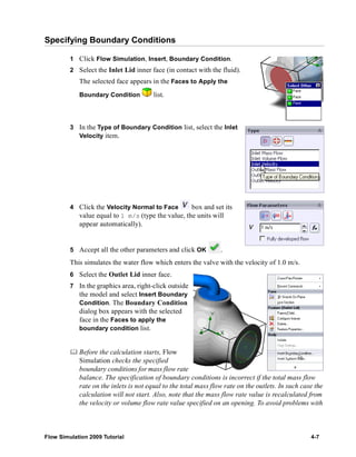
Since the specified conditions are the same for both 40 degrees - long valve and 00
degrees - long valve configurations, it is useful to attach the existing Flow Simulation
project to the 00 degrees - long valve configuration.
Clone the current project to the 00 degrees - long valve
configuration.
Since at zero angle the ball valve becomes a simple straight pipe, there is no need to set the
Minimum gap size value smaller than the default gap size which, in our case, is
automatically set equal to the pipe’s diameter (the automatic minimum gap size depends
on the characteristic size of the faces on which the boundary conditions are set). Note that
using a smaller gap size will result in a finer mesh and, in turn, more computer time and
memory will be required for calculation. To solve your task in the most effective way you
should choose the optimal settings for the task.
Changing the Geometry Resolution
Check to see that the 00 degrees - long valve is the active configuration.
1 Click Flow Simulation, Initial Mesh.
2 Clear the Manual specification of
the minimum gap size check box.
3 Click OK.
Click Flow Simulation, Solve, Run.
Then click Run to start the calculation.
After the calculation is finished, create
the Goal Plot. The goals2 workbook is
created. Go to Excel, then select the both
cells in the Value column and copy them
into the Clipboard.
Goal Name Unit Value Averaged Value Minimum Value
SG Av Total Pressure 1 [Pa] 101805.2057 101804.8525 101801.4794
SG Av Total Pressure 2 [Pa] 102023.7419 102054.9498 102022.7459](https://image.slidesharecdn.com/swflowsimulation2009tutorial-141007202601-conversion-gate02/75/Sw-flowsimulation-2009-tutorial-110-2048.jpg)


![Chapter 5 Cylinder Drag Coefficient
5-14
cylinder 0.01m.SLDPRT [Re 1000]
Goal Name Unit Value Averaged Value Minimum Value Maximum Value
GG X - Component of Force [N] 0.000104929 9.71368E-05 8.75382E-05 0.000105358
Drag Coefficient [ ] 1.023705931 0.94768731 0.85404169 1.027899399
6 Activate the Re 1 configuration and load results. Create the goal plot for both the goals.
cylinder 0.01m.SLDPRT [Re 1]
Goal Name Unit Value Averaged Value Minimum Value Maximum Value
GG X - Component of Force [N] 1.14448E-09 1.16764E-09 1.12756E-09 1.81674E-09
Drag Coefficient [ ] 11.16575499 11.39179479 11.00070462 17.72455528
7 Switch to the cylinder 1m part, activate the Re 1e5 configuration, load results and
create the goal plot for both the goals.
cylinder 1m .SLDPRT [Re 1e5]
Goal Name Unit Value Averaged Value Minimum Value Maximum Value
GG X - Component of Force [N] 0.482967811 0.478070888 0.465937059 0.491484755
Drag Coefficient [ ] 0.471193865 0.46641632 0.454578294 0.47950318
Even if the calculation is steady, the averaged value is more preferred, since in this case
the oscillation effect is of less perceptibility. We will use the averaged goal value for the
other two cases as well.
You can now compare Flow Simulation results with the experimental curve.
0.1 1 10 100 1000 10000 100000 100000
0
Re
1E+07
Ref. 1 Roland L. Panton, “Incompressible flow” Second edition. John Wiley & sons Inc., 1995](https://image.slidesharecdn.com/swflowsimulation2009tutorial-141007202601-conversion-gate02/75/Sw-flowsimulation-2009-tutorial-126-2048.jpg)


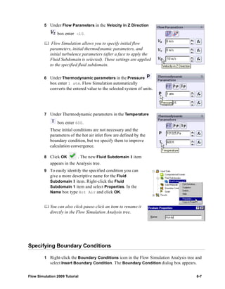
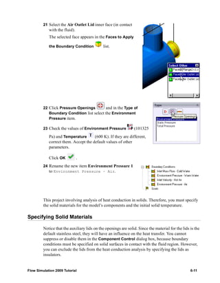
![Chapter 6 Heat Exchanger Efficiency
6-14
Click View, Toolbars, Flow Simulation Display. The
Flow Simulation Display toolbar appears.
The SolidWorks CommandManager is a dynamically-updated, context-sensitive toolbar,
which allows you to save space for the graphics area and access all toolbar buttons from
one location. The tabs below the CommandManager is used to select a specific group of
commands and features to make their toolbar buttons available in the CommandManager.
To get access to the Flow Simulation commands and features, click the Flow Simulation
tab of the CommandManager.
If you wish, you may hide the Flow Simulation toolbars to save the space for the graphics
area, since all necessary commands are available in the CommandManager. To hide a
toolbar, click its name again in the View, Toolbars menu.
1 Click Goals on the Results Main toolbar or CommandManager. The Goals dialog
box appears.
2 Click Add All to select all goals of the project
(actually, in our case there is only one goal) .
3 Click OK. The goals1 Excel workbook is
created.
You can view the average temperature of the tube on the Summary sheet.
Heat Exchanger.SLDASM [Level 3]
Goa l Name Unit Value Ave raged Va lue Minimum Va lue Ma x imum V alue Progre ss [%] Use In Convergence
VG Av T of Tube [K] 328.4682387 327.4703038 324.7176733 328.4682387 100 Yes
Iterations: 51
Analysis in terval: 21
Creating a Cut Plot
1 Click Cut Plot on the Flow Simulation Results Features toolbar. The Cut Plot
dialog box appears.](https://image.slidesharecdn.com/swflowsimulation2009tutorial-141007202601-conversion-gate02/75/Sw-flowsimulation-2009-tutorial-140-2048.jpg)


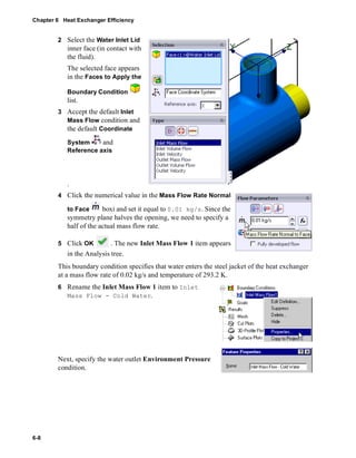
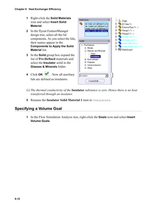
![Chapter 10 Non-Newtonian Flow in a Channel with Cylinders
10-4
Run the calculation. When the calculation is finished, create the goal plot to obtain the
pressure drop between the channel’s inlet and outlet.
Array o f C ylinders.SLDPRT [XGS]
Go a l Nam e Unit Va lue Ave ra ge d Va lue Minim um V a lue Ma x im um V a lue Progre ss [%]
SG A v Total P res sure 1 [P a] 105622.4926 105622.4125 105620.3901 105627.4631 100
SG A v Total P res sure 2 [P a] 101329.0109 101329.0091 101329.0051 101329.0109 100
Pres sure Drop [P a] 4293.481659 4293.4034 4298.457377 4291.380166 100
It is seen that the channel's total pressure loss is about 4 kPa.
Comparison with Water
Let us now consider the flow of water in the same channel under the same conditions (at
the same volume flow rate).
Create a new configuration by cloning the current
project, and name it Water.
Changing Project Settings
1 Click Flow Simulation, General
Settings.
2 On the Navigator click Fluids.
3 In the Project Fluids table, select
XGum and click Remove. Answer
OK to the appearing warning
message.
4 Select Water in Liquids and click
Add.
5 Under Flow Characteristics, change
Flow type to Laminar and Turbulent.
6 Click OK.
Run the calculation. After the calculation is finished, create the goal plot.](https://image.slidesharecdn.com/swflowsimulation2009tutorial-141007202601-conversion-gate02/75/Sw-flowsimulation-2009-tutorial-206-2048.jpg)
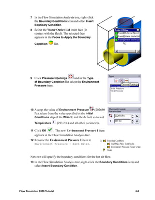
![Array o f C ylinders.SLDPRT [water]
Go a l Nam e Unit Va lue Ave ra ge d Va lue Minim um V a lue Ma x im um V a lue Progre ss [%]
SG A v Total P res sure 1 [P a] 101395.004 101395.0214 101394.8731 101395.1171 100
SG A v Total P res sure 2 [P a] 101329.3912 101329.3378 101329.3084 101329.3912 100
Pres sure Drop [P a] 65.6128767 65.68357061 65.76566097 65.55243288 100
As shown in the results table above, the channel's total pressure loss is about 60 Pa, i.e.
60...70 times lower than with the 3% aqueous solution of xanthan gum, this is due to the
water's much smaller viscosity under the problem's flow shear rates.
The XGS (above) and water velocity distribution in the range from 0 to 30 cm/s.
1 Georgiou G., Momani S., Crochet M.J., and Walters K. Newtonian and Non-Newtonian
Flow in a Channel Obstructed by an Antisymmetric Array of Cylinders. Journal of
Non-Newtonian Fluid Mechanics, v.40 (1991), p.p. 231-260.
Flow Simulation 2009 Tutorial 10-5](https://image.slidesharecdn.com/swflowsimulation2009tutorial-141007202601-conversion-gate02/75/Sw-flowsimulation-2009-tutorial-207-2048.jpg)


![The flow pressure distribution
For the impeller under consideration the obtained efficiency is 0.79.
Goal Name Unit Value Averaged Value Minimum Value Maximum Value
Efficiency [ ] 0.787039615 0.786371 0.784334 0.787117
Flow Simulation 2009 Tutorial 12-9](https://image.slidesharecdn.com/swflowsimulation2009tutorial-141007202601-conversion-gate02/75/Sw-flowsimulation-2009-tutorial-227-2048.jpg)


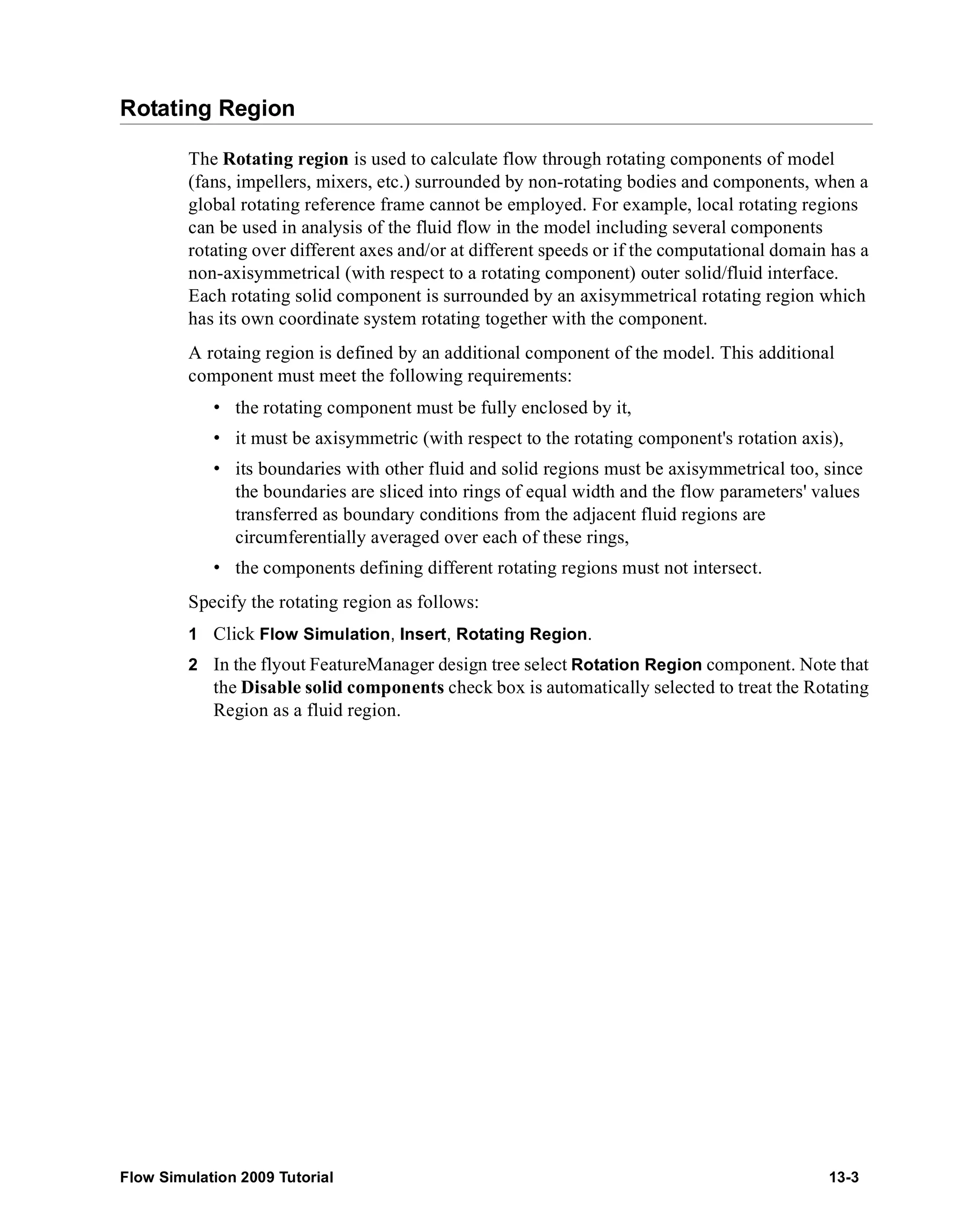
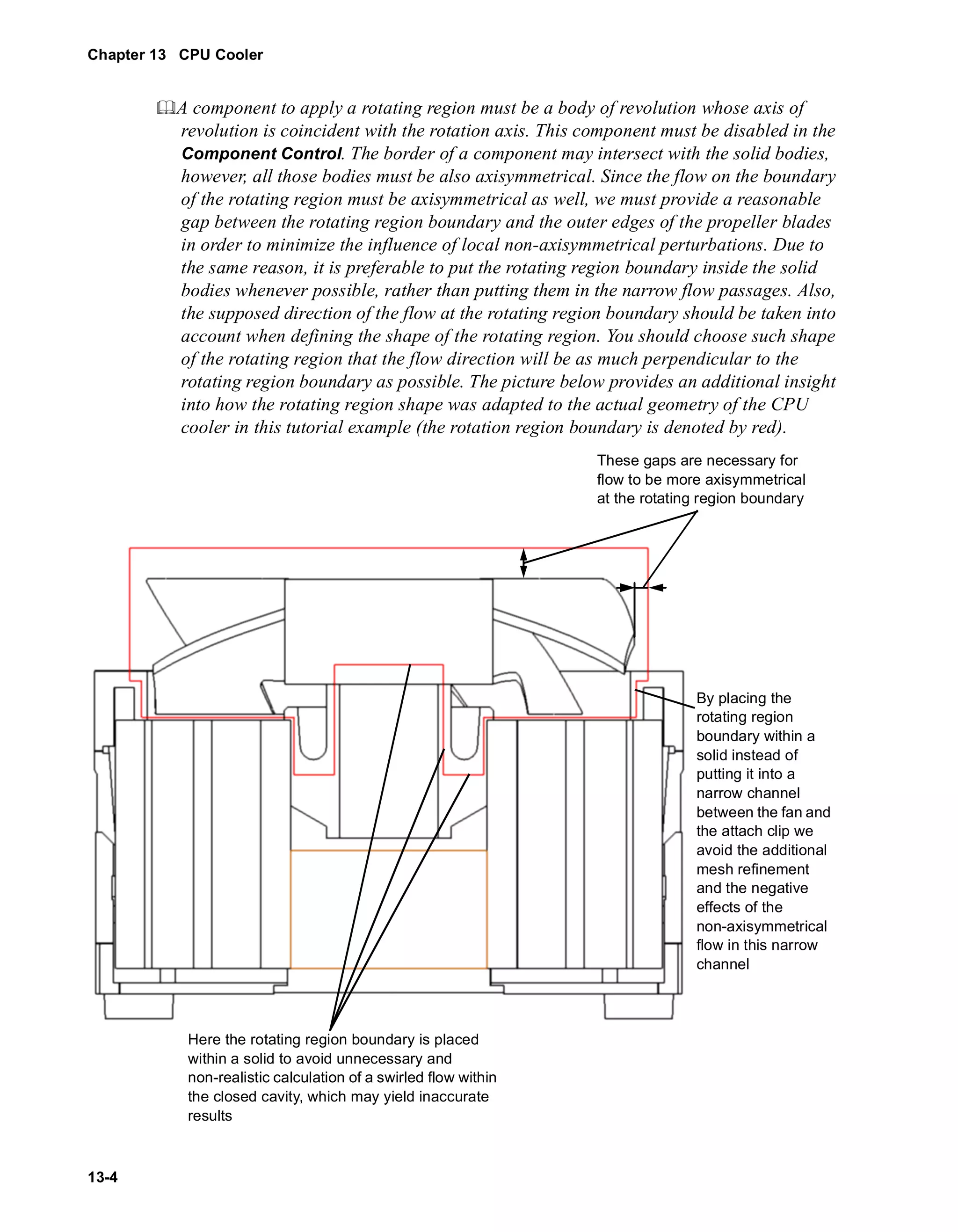
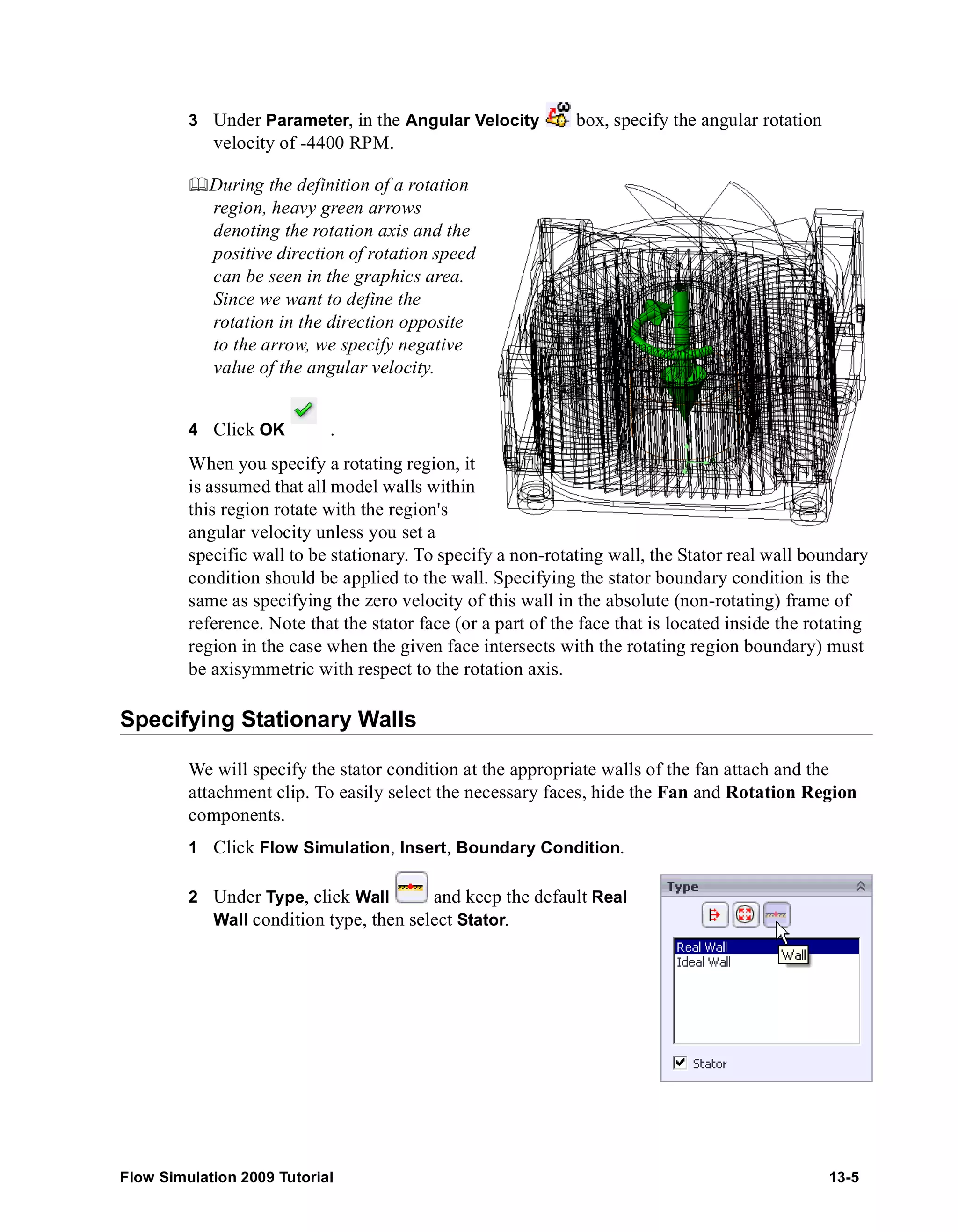
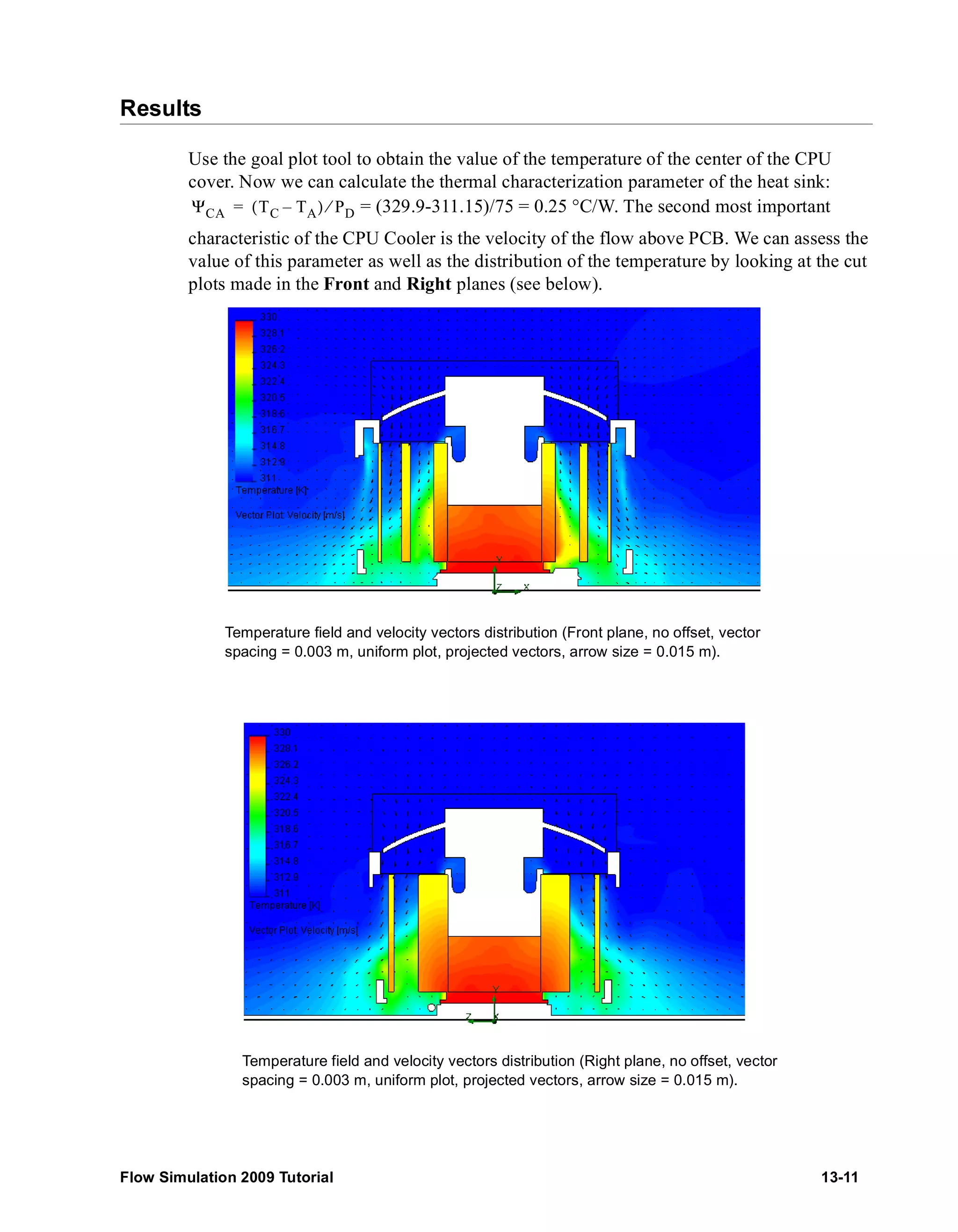
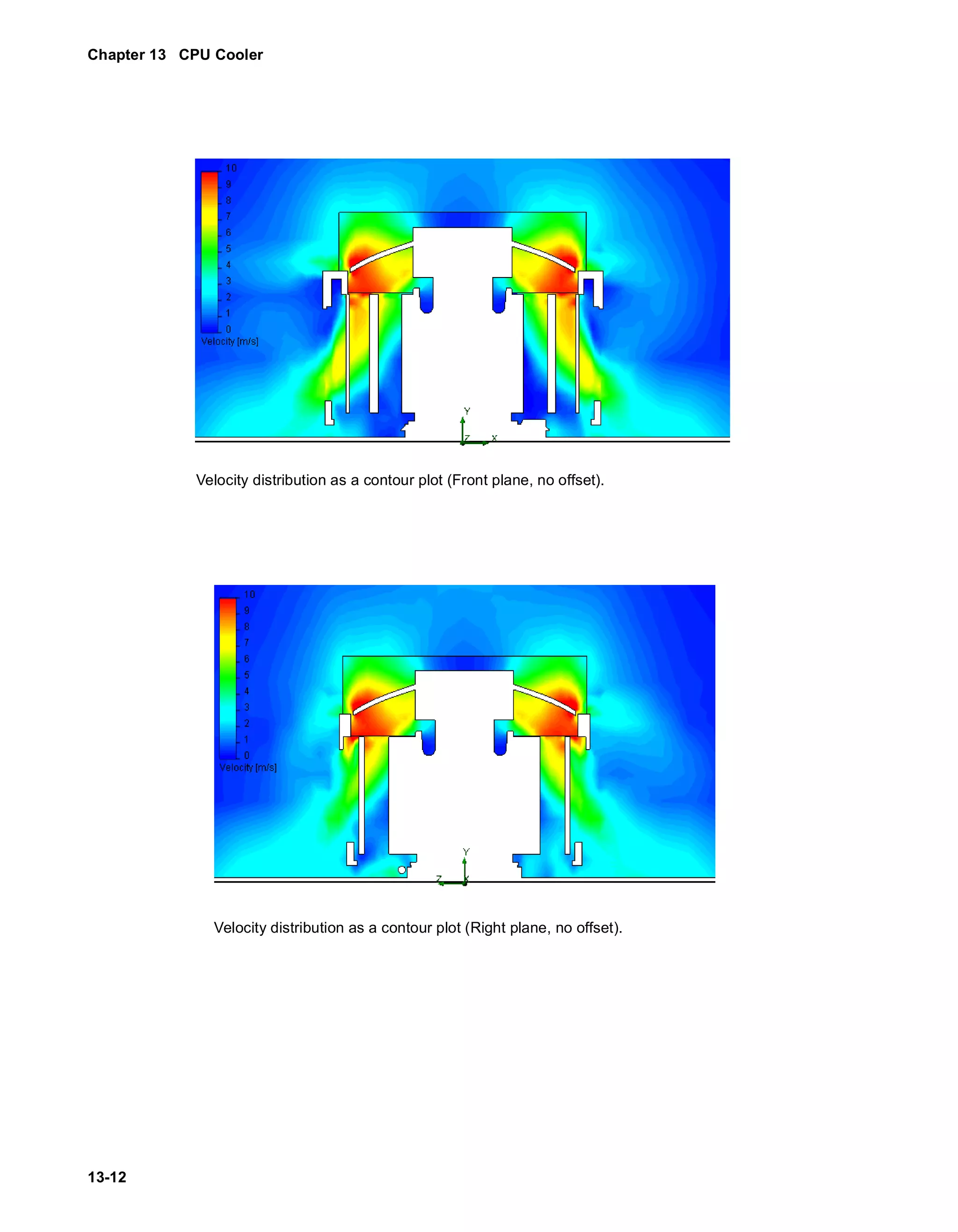

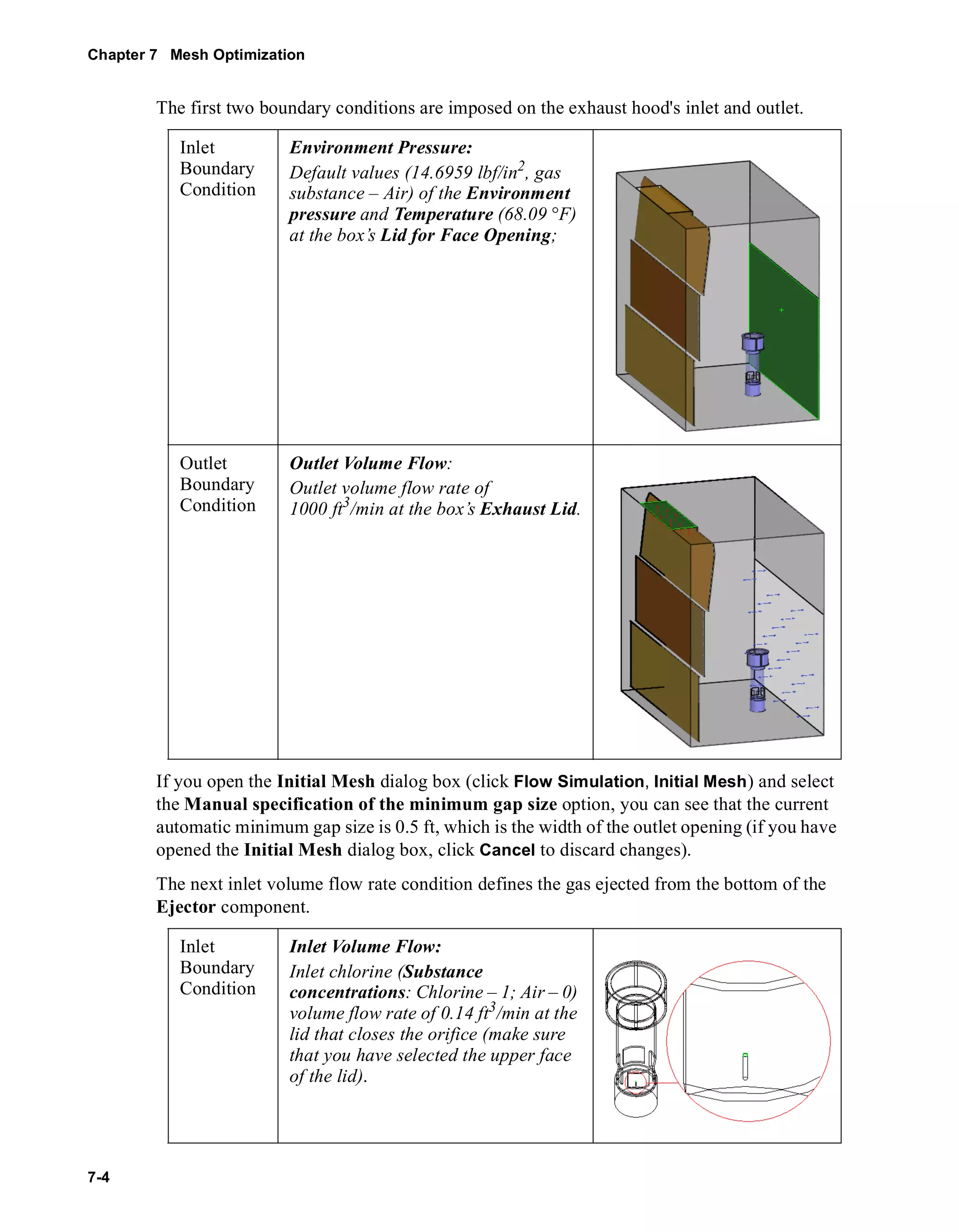
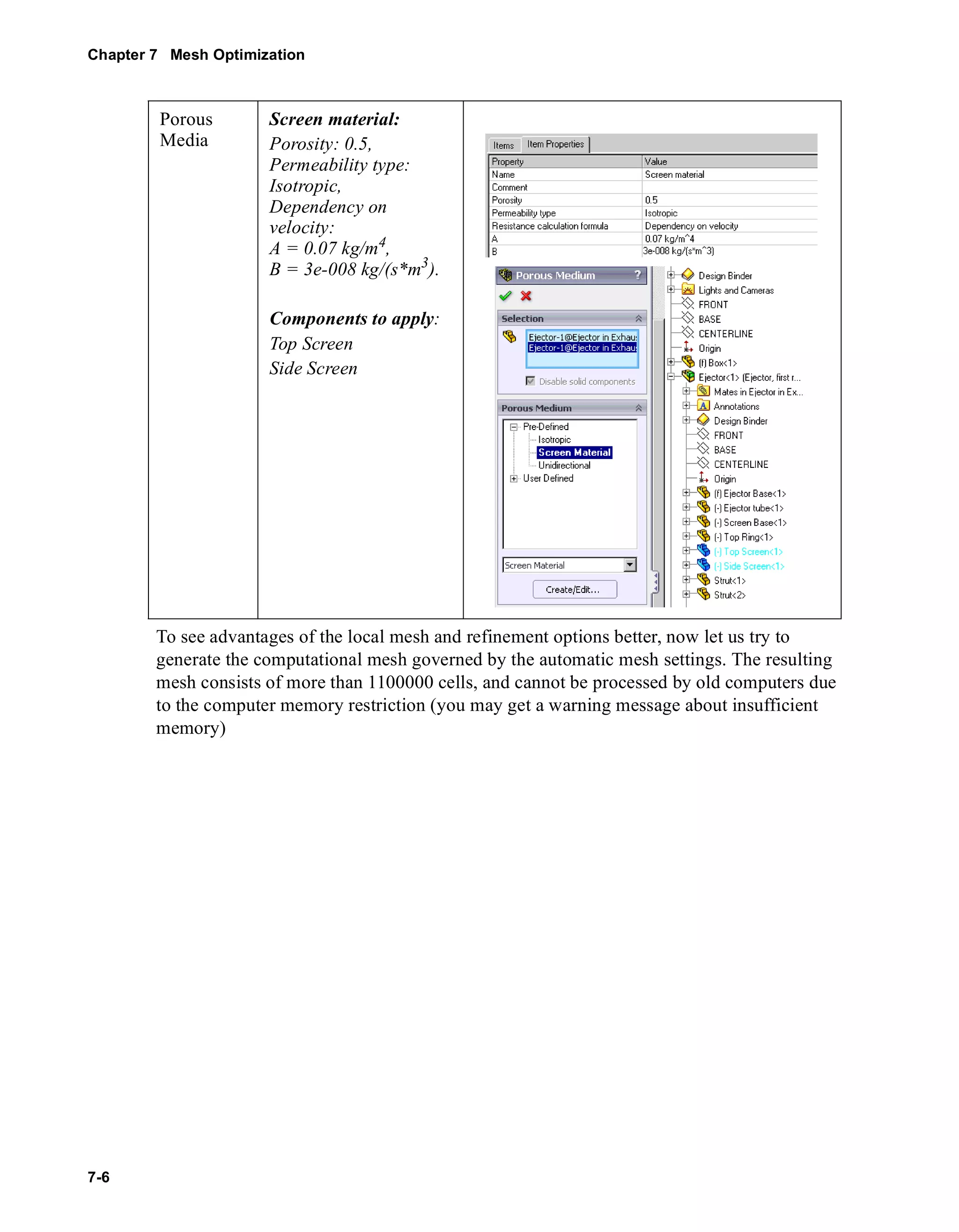
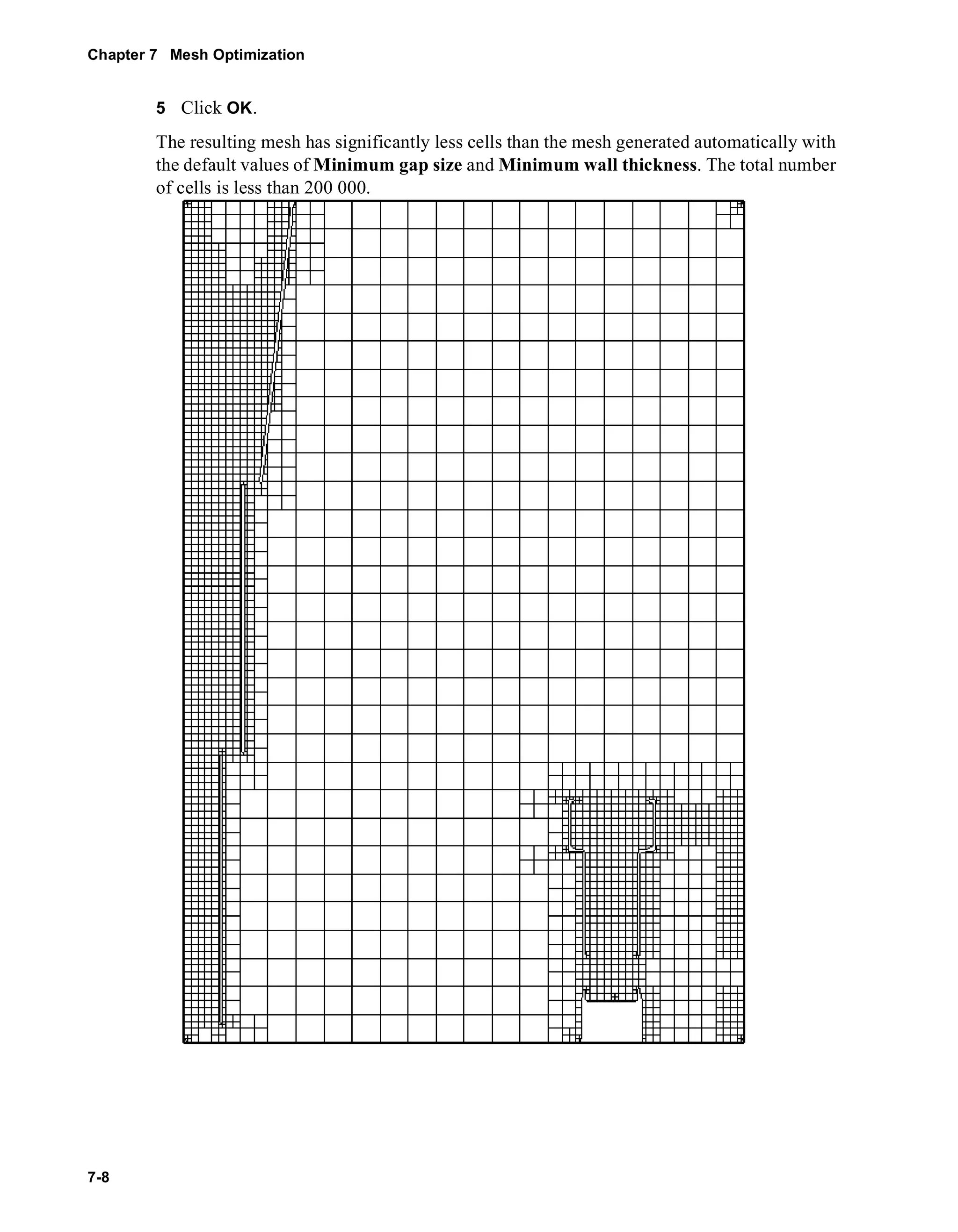
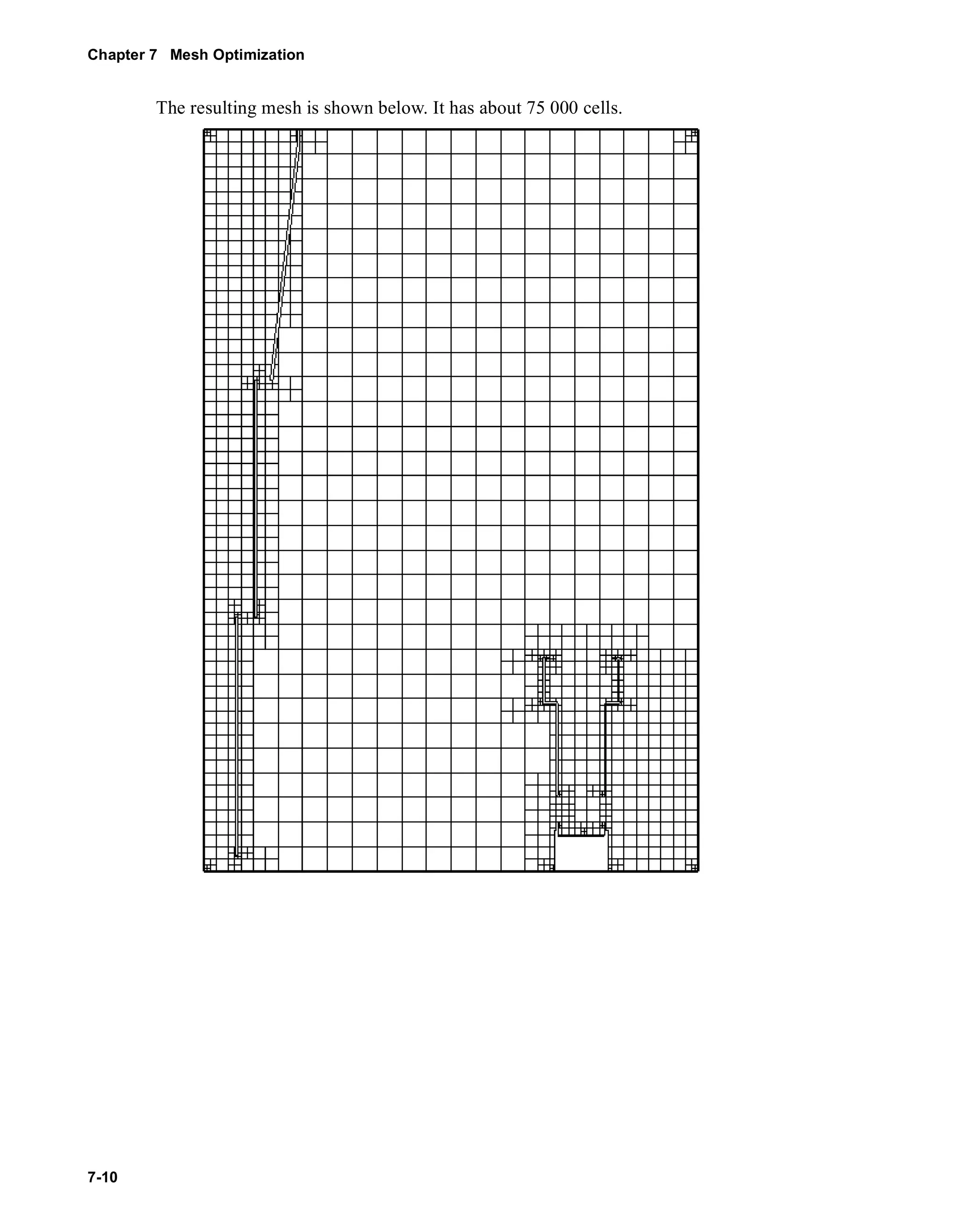
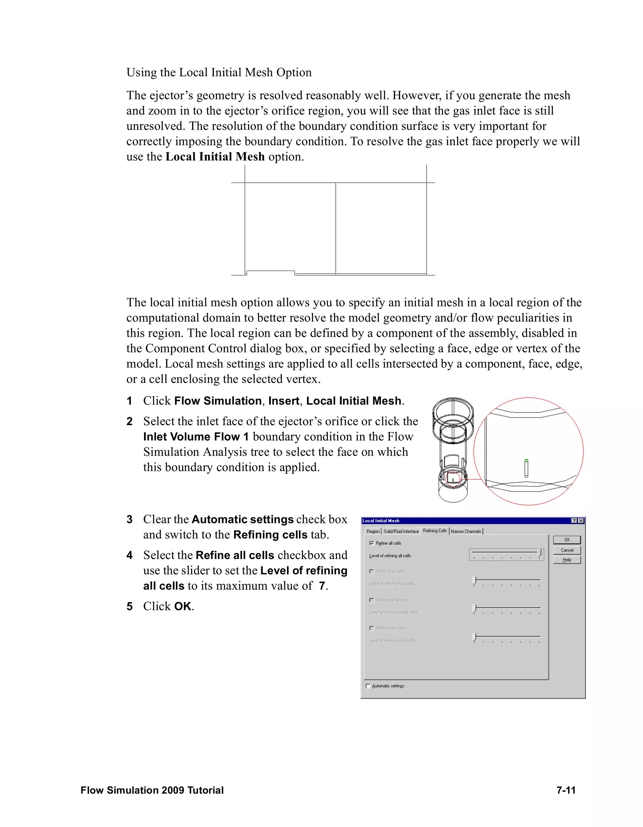
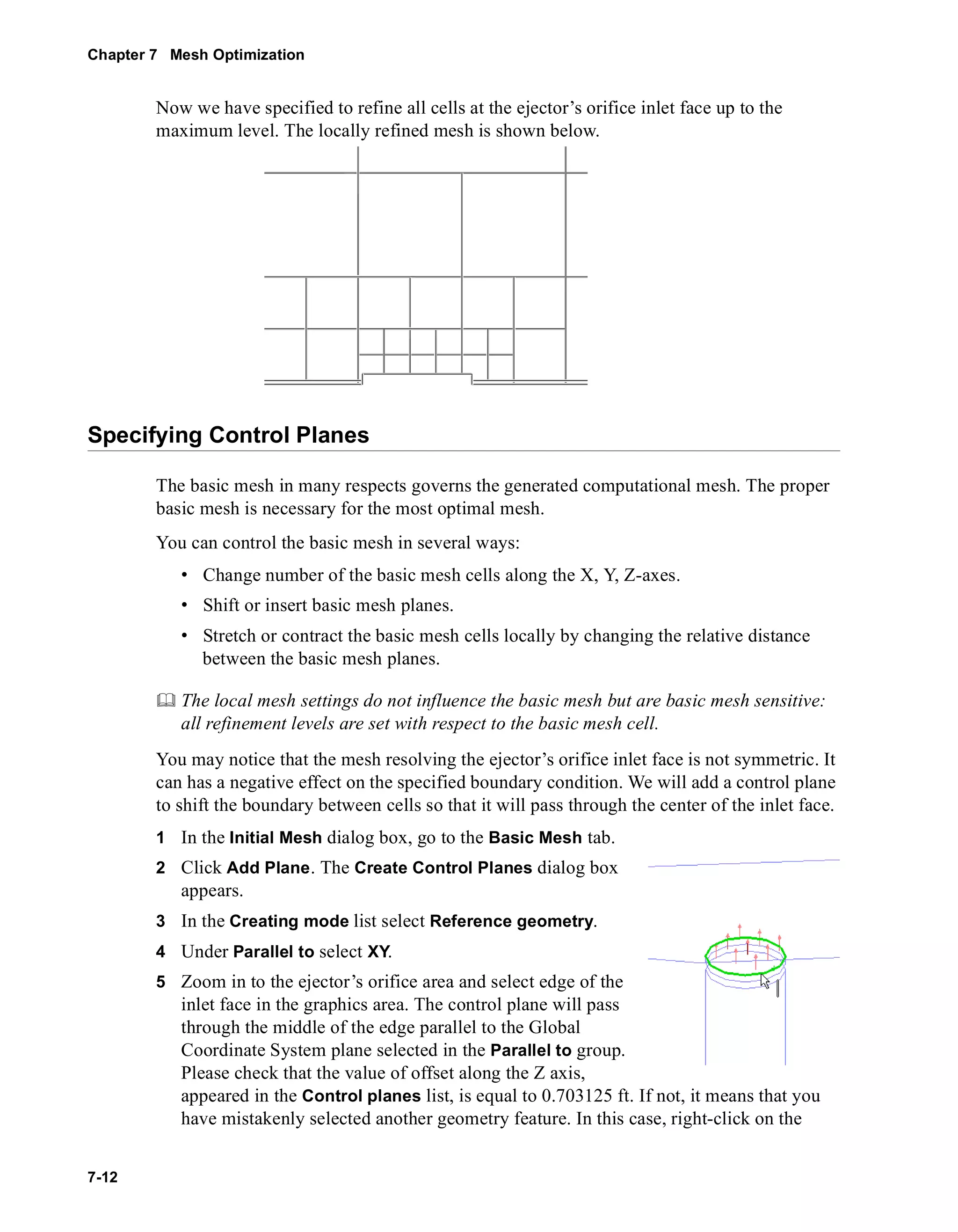
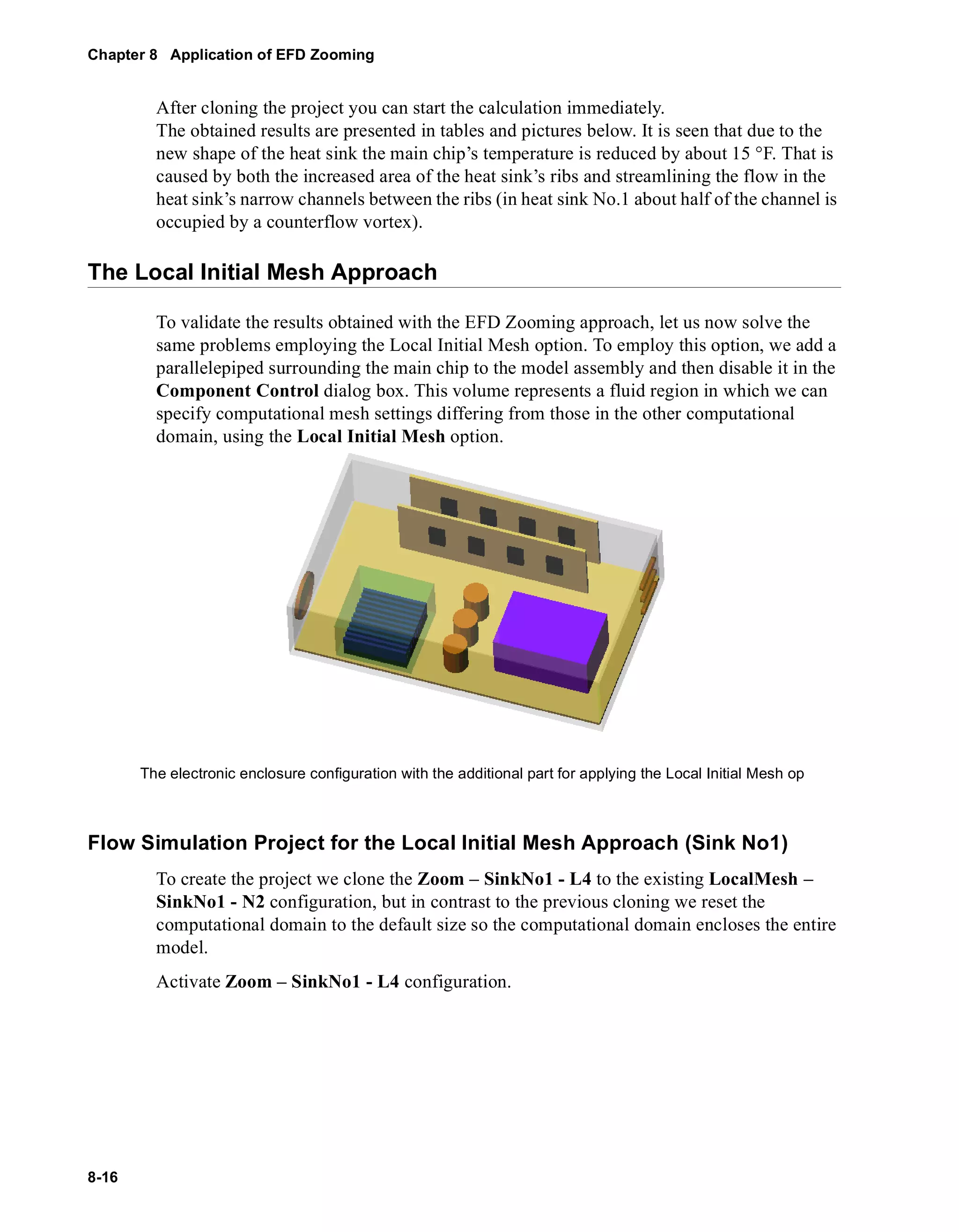
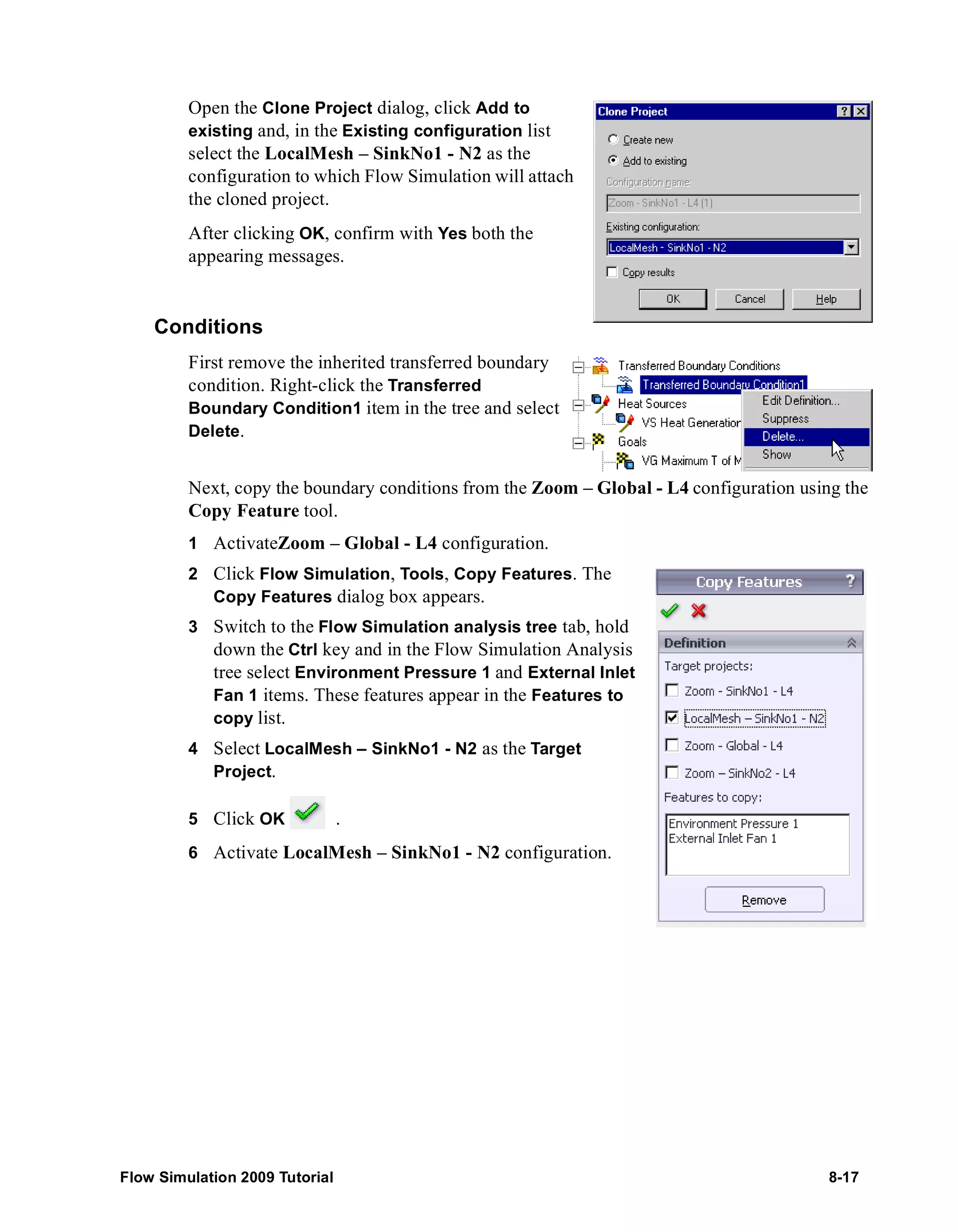
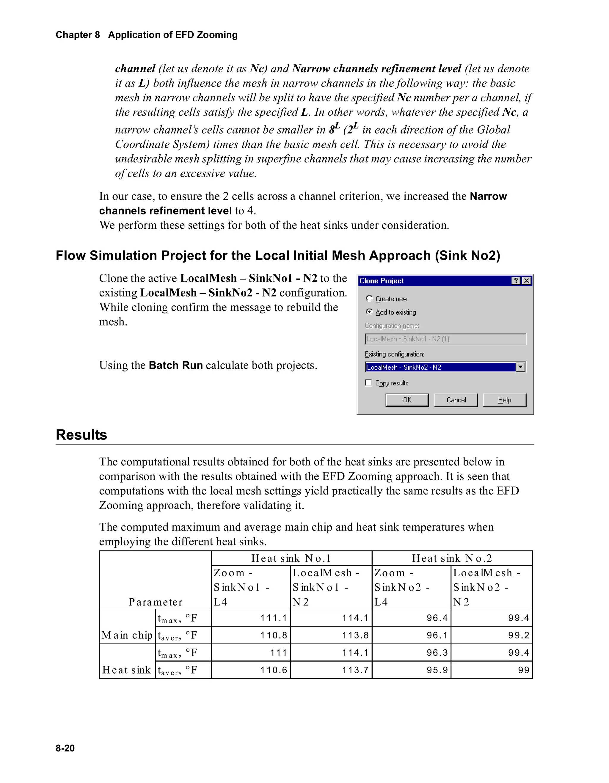
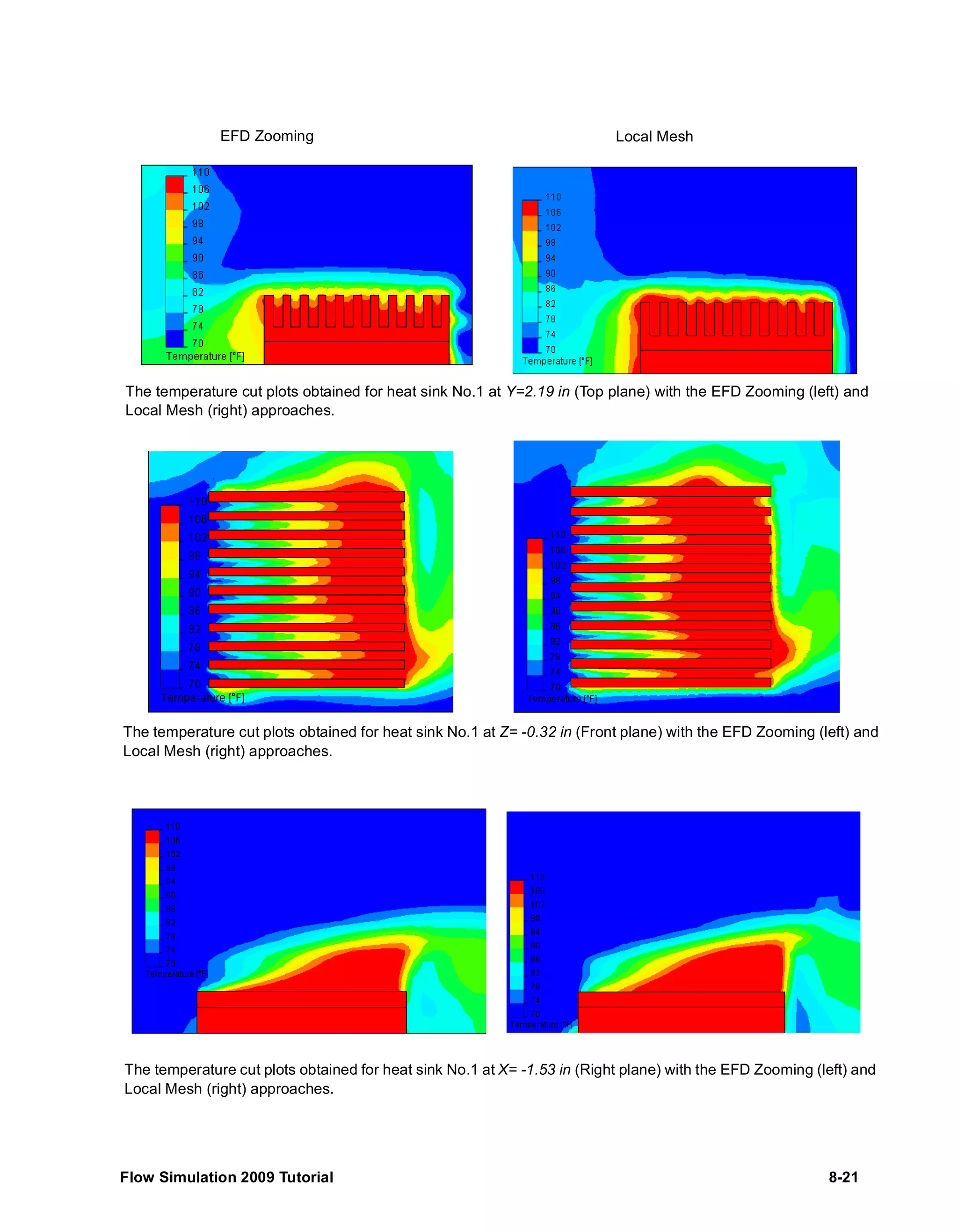
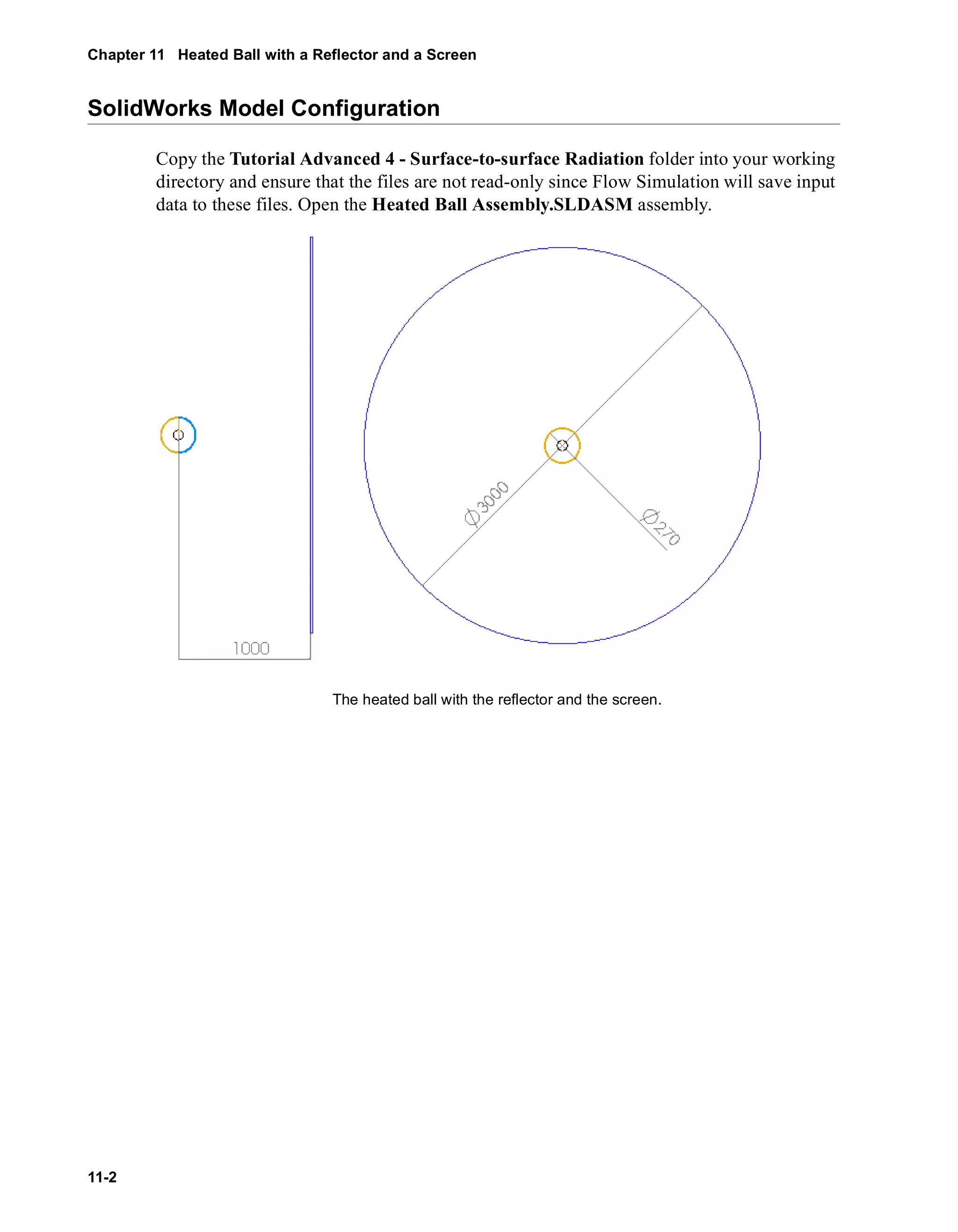
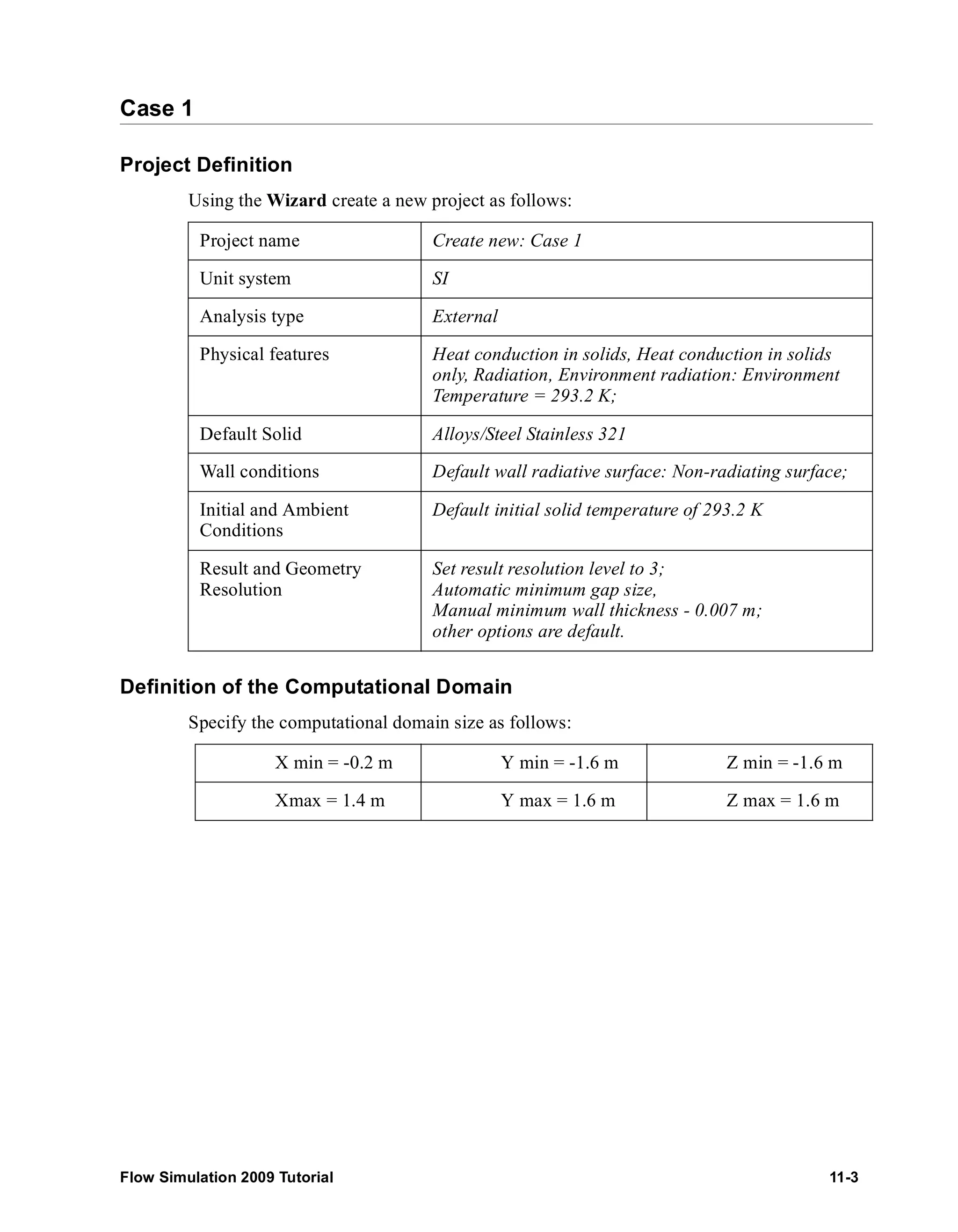
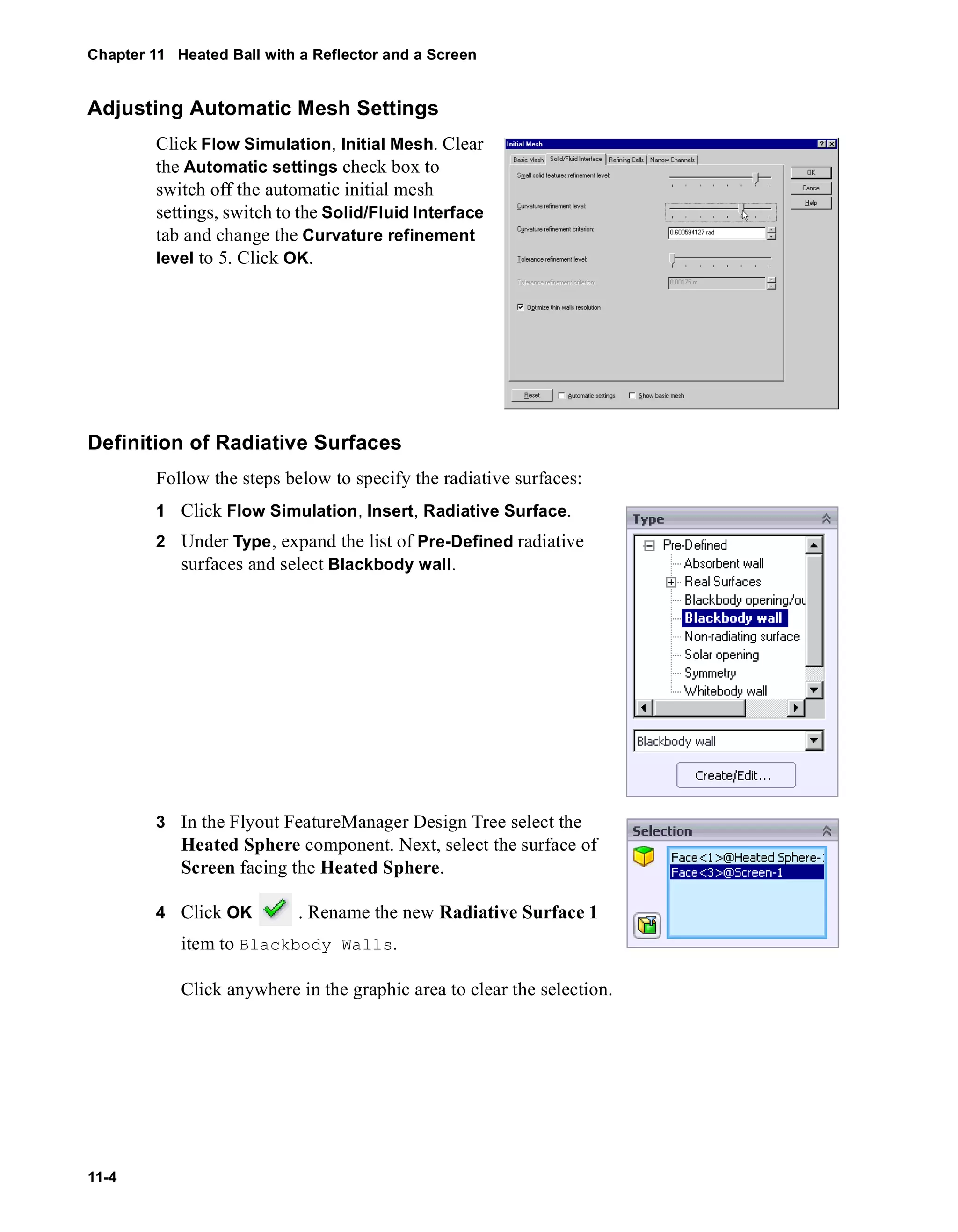
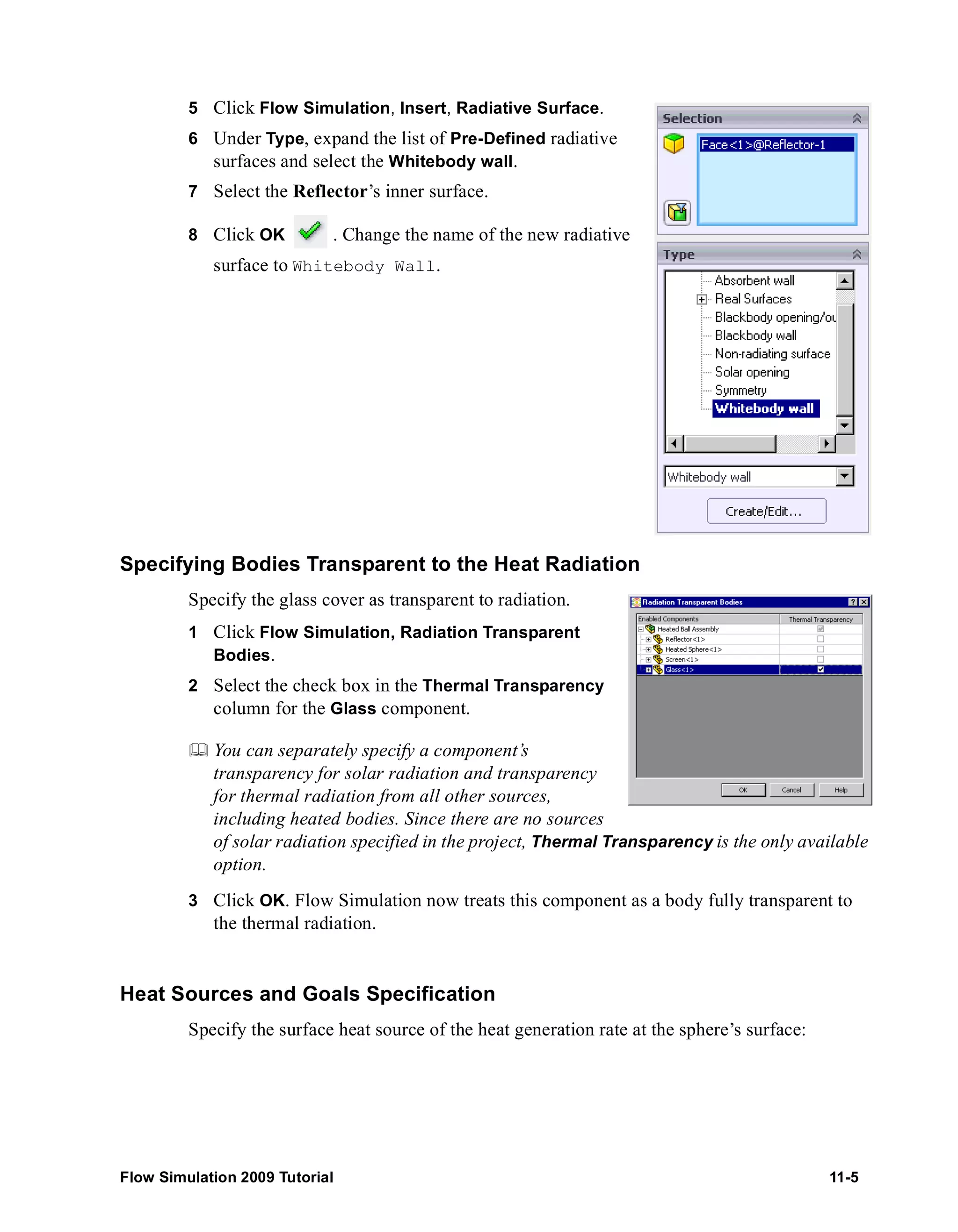
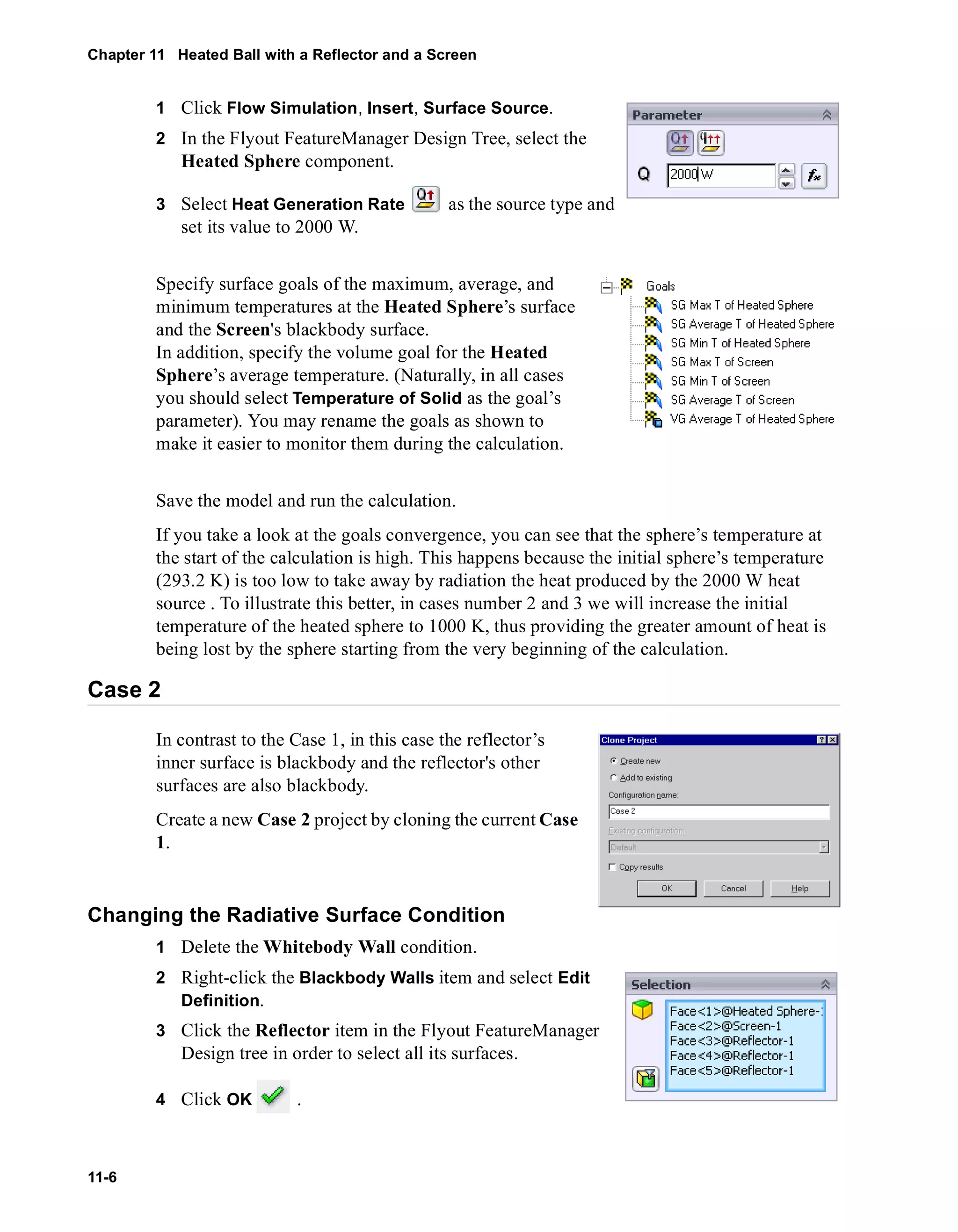
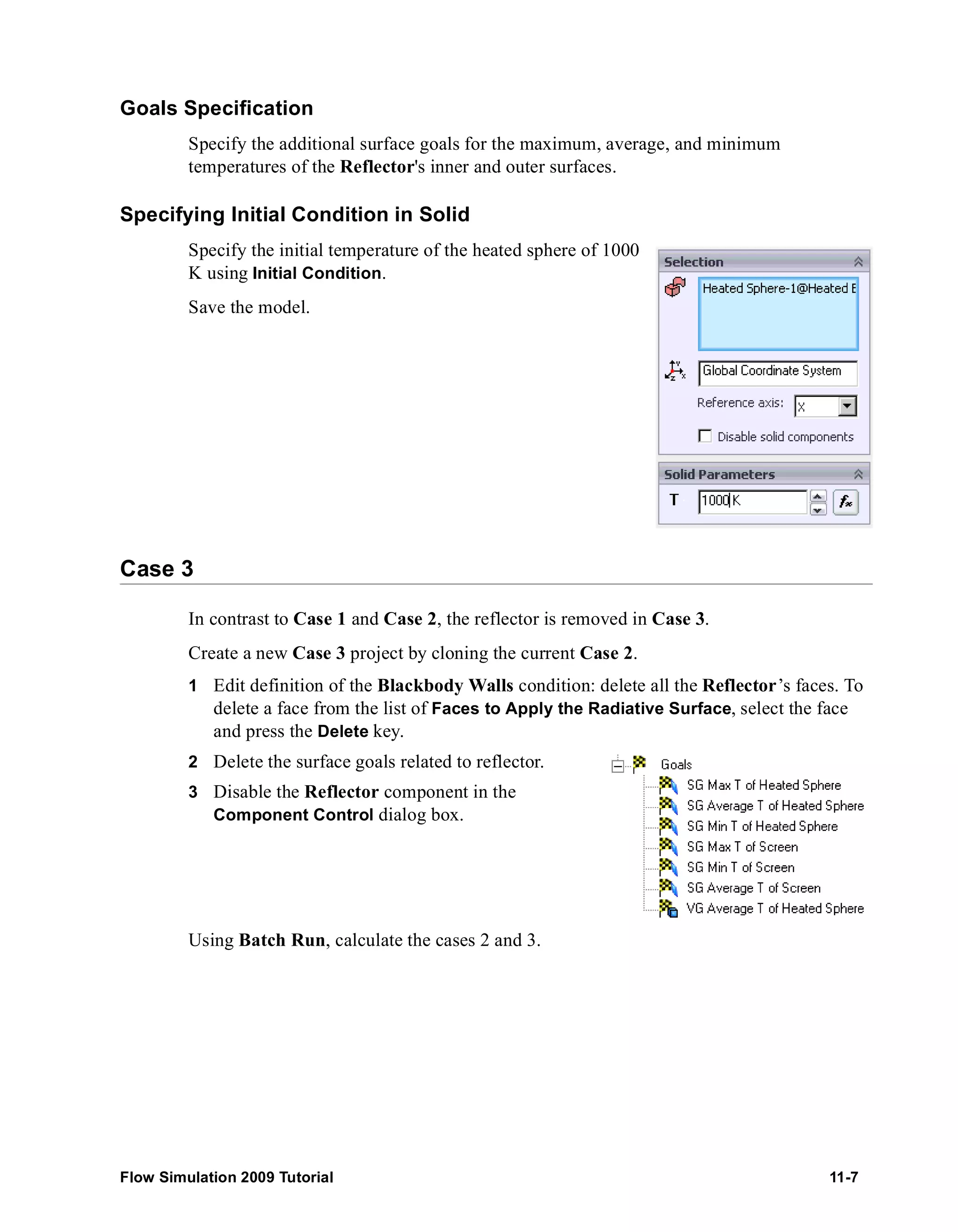
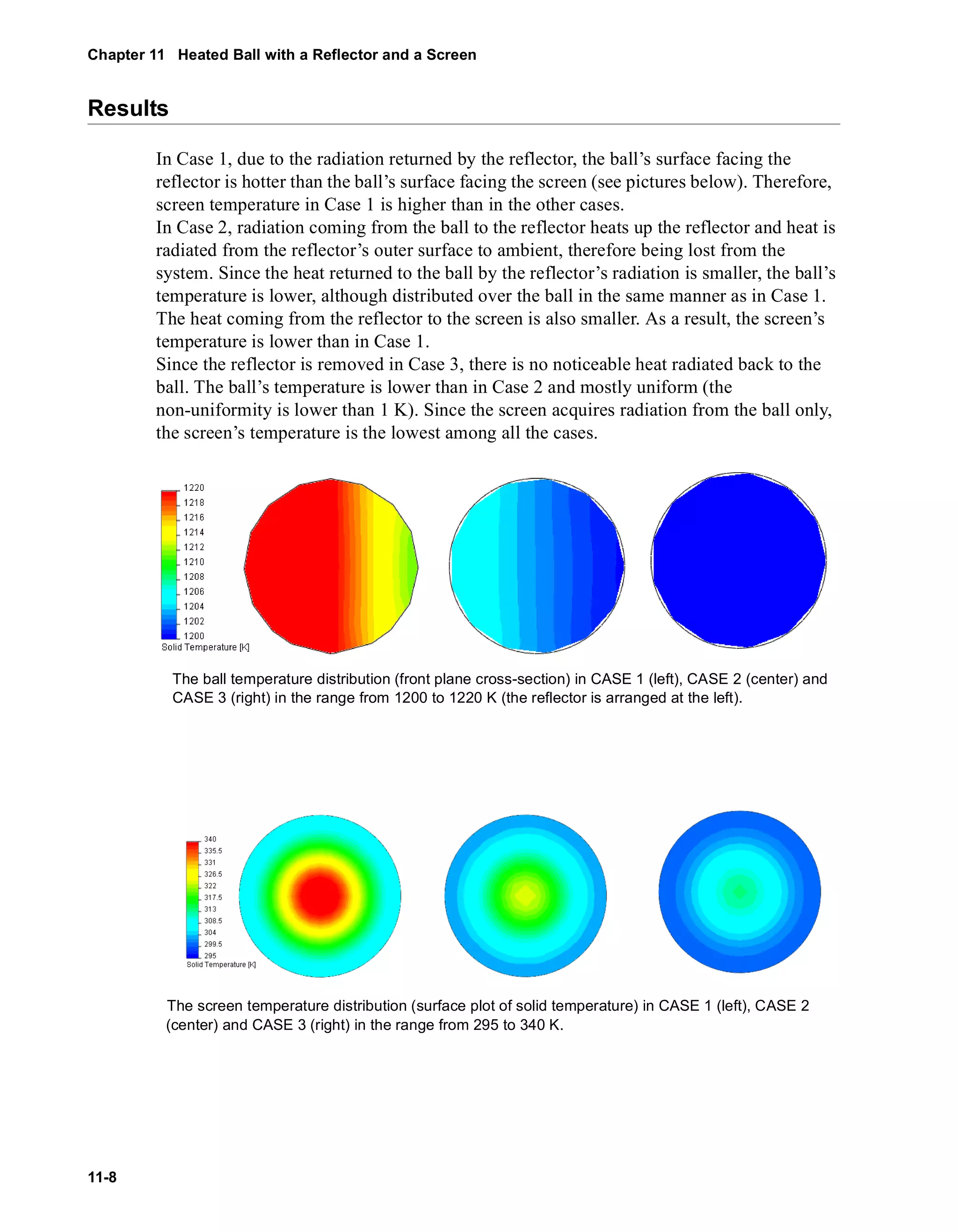
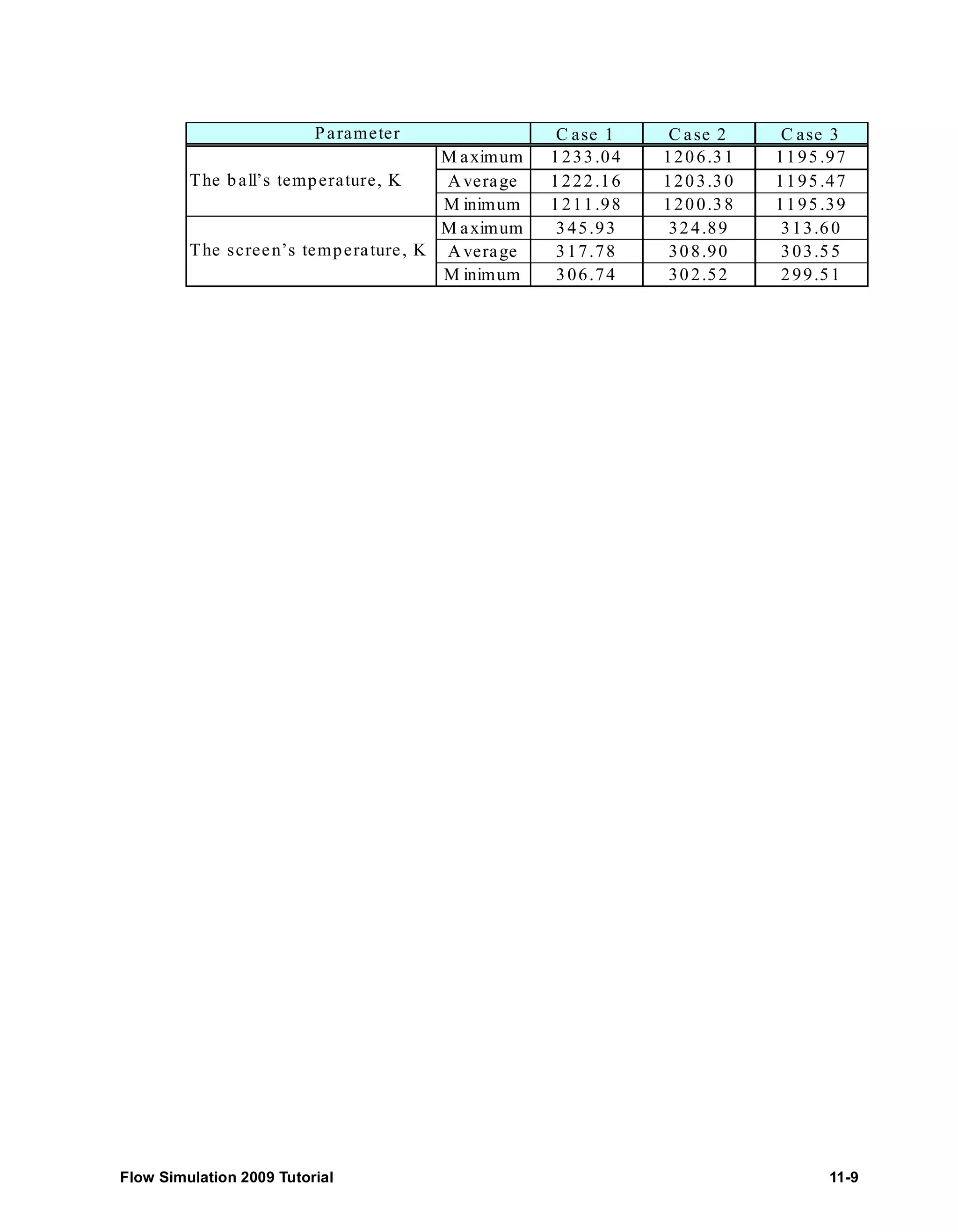
The document provides a detailed tutorial on using SolidWorks Flow Simulation 2009, focusing on various aspects such as creating flow simulation projects, setting up boundary conditions, defining engineering goals, and utilizing different plotting techniques. It also covers advanced topics like conjugate heat transfer and porous media simulations, along with instructions for monitoring and analyzing simulation results. Each section includes step-by-step procedures for improving user understanding of the software and optimizing flow simulation outcomes.


![[Julien boisset] solidworks_simulation_2009_validation](https://cdn.slidesharecdn.com/ss_thumbnails/julienboissetsolidworkssimulation2009validation-150503100431-conversion-gate01-thumbnail.jpg?width=600ounds&width=560&fit=bounds)


