Key procedures tobe defined
• EXPAND
– Generate all successor nodes of a given node
• GOAL-TEST
– Test if state satisfies all goal conditions
• QUEUEING-FUNCTION
– Used to maintain a ranked list of nodes that are
candidates for expansion
5.
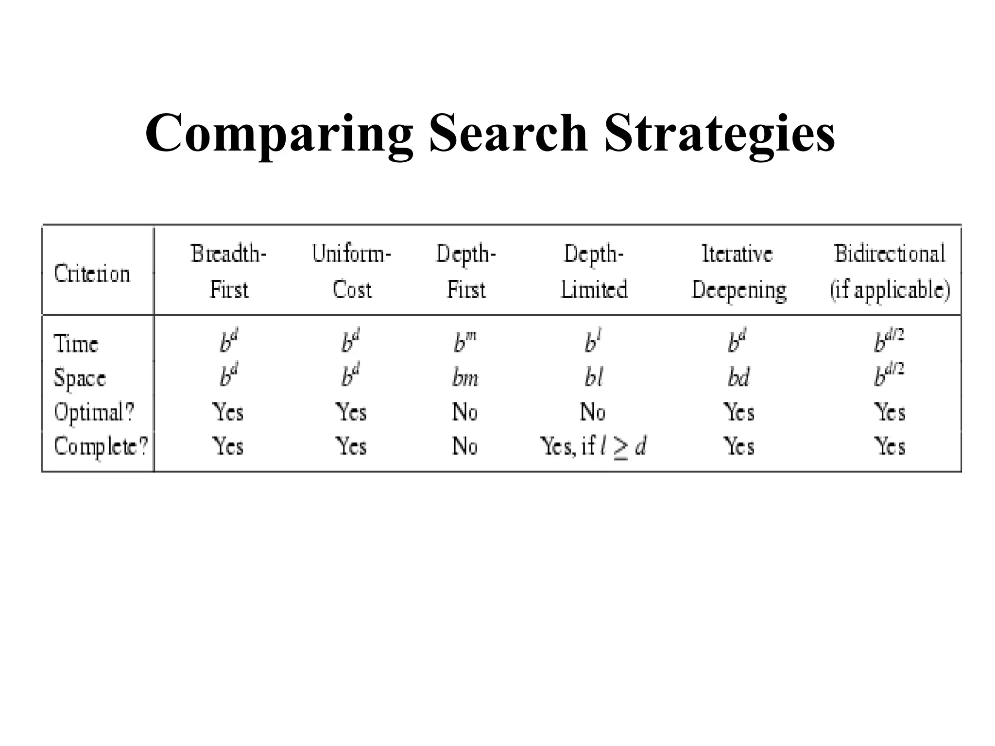
Uninformed vs. InformedSearch
• Uninformed search strategies
– Also known as “blind search,” uninformed search strategies use no
information about the likely “direction” of the goal node(s)
– Uninformed search methods: Breadth-first, depth-first, depth-
limited, uniform-cost, depth-first iterative deepening, bidirectional
• Informed search strategies (next class...)
– Also known as “heuristic search,” informed search strategies use
information about the domain to (try to) (usually) head in the
general direction of the goal node(s)
– Informed search methods: Hill climbing, best-first, greedy search,
beam search, A, A*
6.
Breadth-First
• Enqueue nodeson nodes in FIFO (first-in, first-out) order.
• Complete
• Optimal (i.e., admissible) if all operators have the same cost. Otherwise, not optimal but
finds solution with shortest path length.
• Exponential time and space complexity, O(bd
), where d is the depth of the solution and b is
the branching factor (i.e., number of children) at each node
• Will take a long time to find solutions with a large number of steps because must look at all
shorter length possibilities first
– A complete search tree of depth d where each non-leaf node has b children, has a total of 1 + b + b2
+ ... + bd
= (b(d+1)
- 1)/(b-1) nodes
– For a complete search tree of depth 12, where every node at depths 0, ..., 11 has 10 children and
every node at depth 12 has 0 children, there are 1 + 10 + 100 + 1000 + ... + 1012
= (1013
- 1)/9 =
O(1012
) nodes in the complete search tree. If BFS expands 1000 nodes/sec and each node uses 100
bytes of storage, then BFS will take 35 years to run in the worst case, and it will use 111 terabytes of
memory!
7.
Depth-First (DFS)
• Enqueuenodes on nodes in LIFO (last-in, first-out) order. That is,
nodes used as a stack data structure to order nodes.
• May not terminate without a “depth bound,” i.e., cutting off search
below a fixed depth D ( “depth-limited search”)
• Not complete (with or without cycle detection, and with or without a
cutoff depth)
• Exponential time, O(bd
), but only linear space, O(bd)
• Can find long solutions quickly if lucky (and short solutions slowly if
unlucky!)
• When search hits a deadend, can only back up one level at a time even
if the “problem” occurs because of a bad operator choice near the top of
the tree. Hence, only does “chronological backtracking”
8.
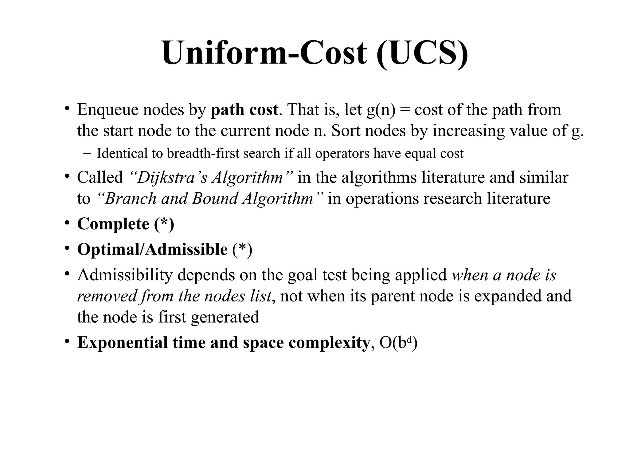
Uniform-Cost (UCS)
• Enqueuenodes by path cost. That is, let g(n) = cost of the path from
the start node to the current node n. Sort nodes by increasing value of g.
– Identical to breadth-first search if all operators have equal cost
• Called “Dijkstra’s Algorithm” in the algorithms literature and similar
to “Branch and Bound Algorithm” in operations research literature
• Complete (*)
• Optimal/Admissible (*)
• Admissibility depends on the goal test being applied when a node is
removed from the nodes list, not when its parent node is expanded and
the node is first generated
• Exponential time and space complexity, O(bd
)
9.
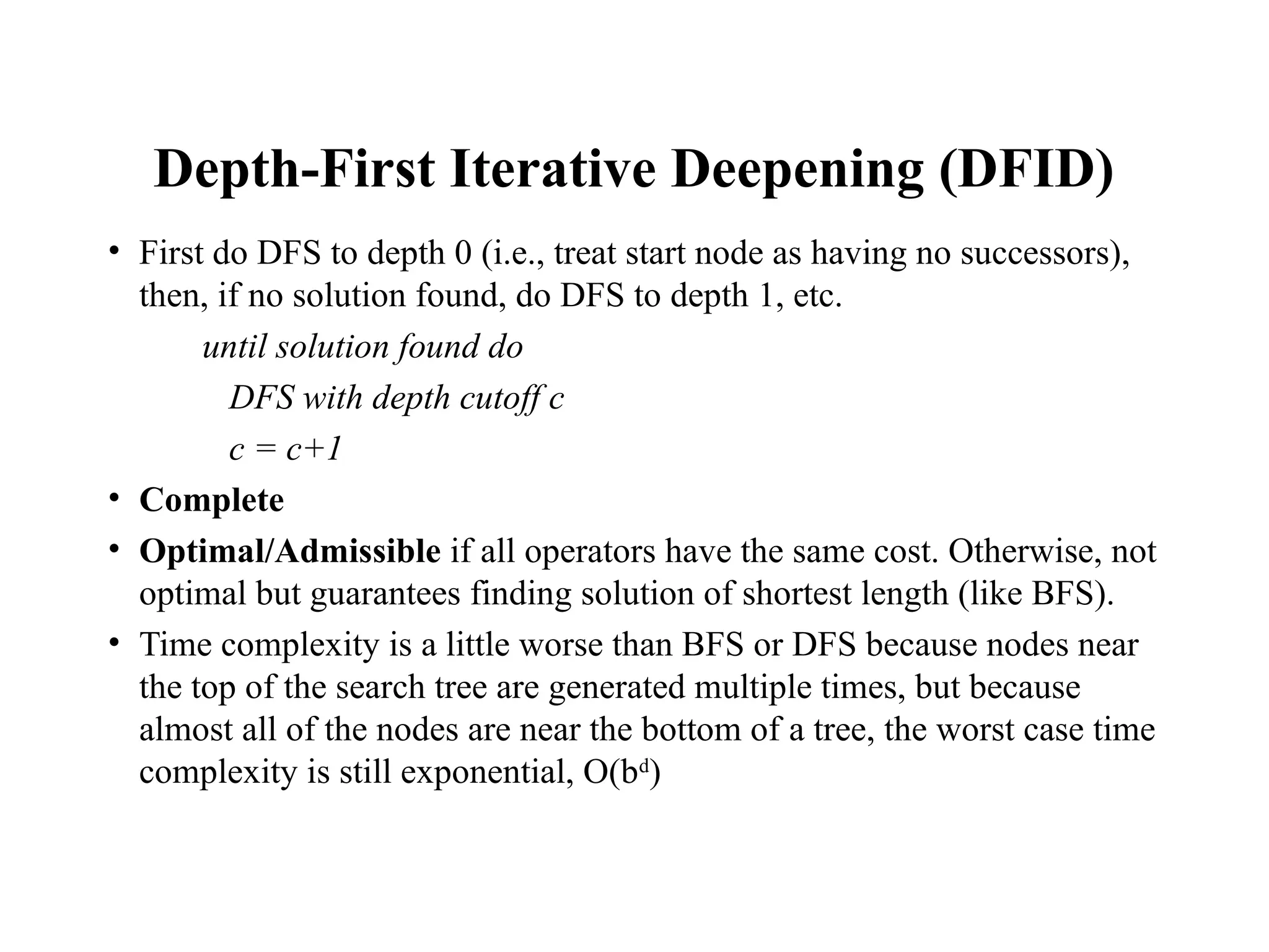
Depth-First Iterative Deepening(DFID)
• First do DFS to depth 0 (i.e., treat start node as having no successors),
then, if no solution found, do DFS to depth 1, etc.
until solution found do
DFS with depth cutoff c
c = c+1
• Complete
• Optimal/Admissible if all operators have the same cost. Otherwise, not
optimal but guarantees finding solution of shortest length (like BFS).
• Time complexity is a little worse than BFS or DFS because nodes near
the top of the search tree are generated multiple times, but because
almost all of the nodes are near the bottom of a tree, the worst case time
complexity is still exponential, O(bd
)
10.
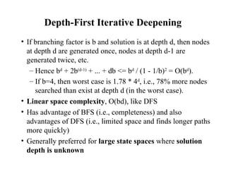
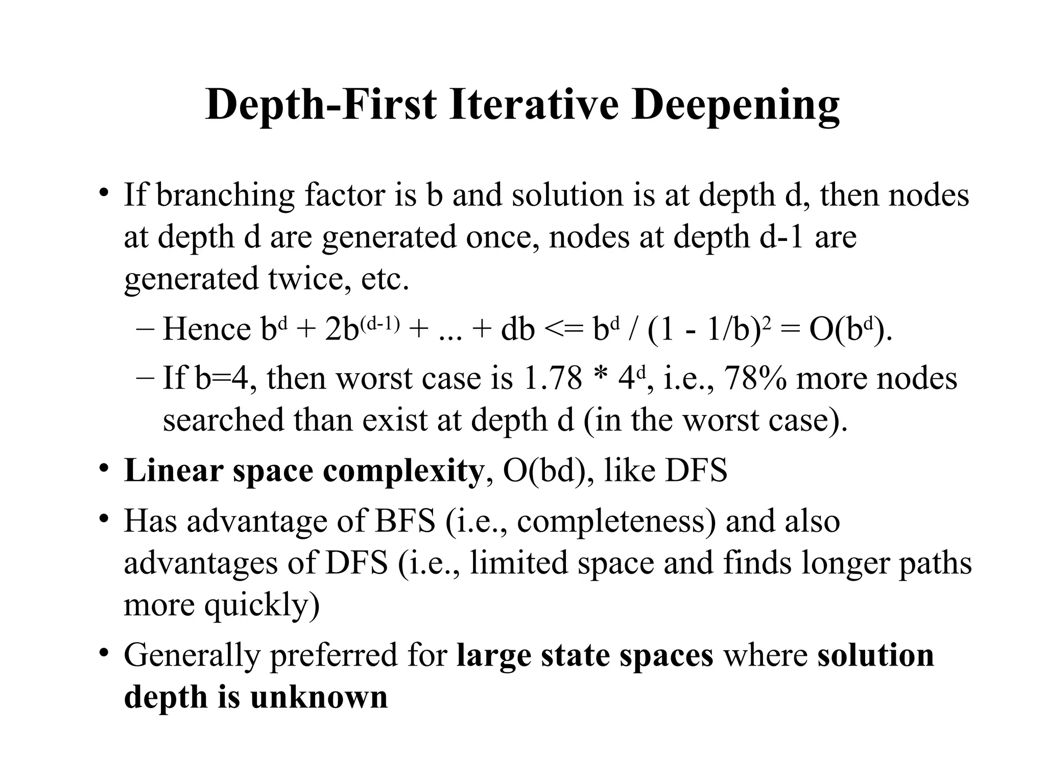
Depth-First Iterative Deepening
•If branching factor is b and solution is at depth d, then nodes
at depth d are generated once, nodes at depth d-1 are
generated twice, etc.
– Hence bd
+ 2b(d-1)
+ ... + db <= bd
/ (1 - 1/b)2
= O(bd
).
– If b=4, then worst case is 1.78 * 4d
, i.e., 78% more nodes
searched than exist at depth d (in the worst case).
• Linear space complexity, O(bd), like DFS
• Has advantage of BFS (i.e., completeness) and also
advantages of DFS (i.e., limited space and finds longer paths
more quickly)
• Generally preferred for large state spaces where solution
depth is unknown
11.
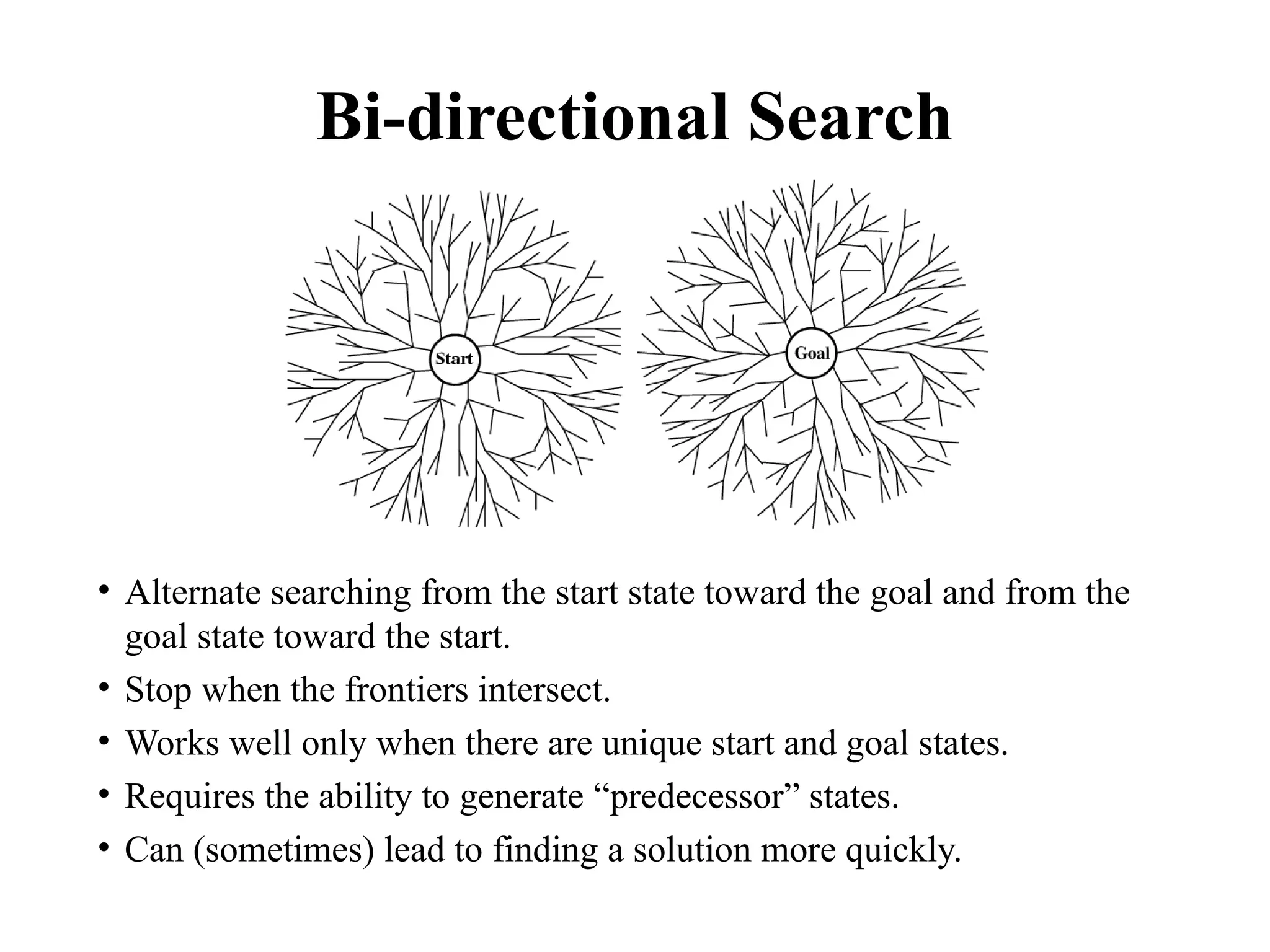
Bi-directional Search
• Alternatesearching from the start state toward the goal and from the
goal state toward the start.
• Stop when the frontiers intersect.
• Works well only when there are unique start and goal states.
• Requires the ability to generate “predecessor” states.
• Can (sometimes) lead to finding a solution more quickly.
Avoiding Repeated States
•In increasing order of effectiveness in reducing size
of state space and with increasing computational
costs:
1. Do not return to the state you just came from.
2. Do not create paths with cycles in them.
3. Do not generate any state that was ever created
before.
• Net effect depends on frequency of “loops” in state
space.
14.
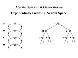
A State Spacethat Generates an
Exponentially Growing Search Space
15.
Holy Grail Search
Wouldn’tit be nice if we could go straight to the solution,
without any wasted detours off to the side?
If only we knew where we were headed…
16.
Informed Methods Add
Domain-SpecificInformation
• Add domain-specific information to select the best
path along which to continue searching
• Define a heuristic function h(n) that estimates the
“goodness” of a node n.
– Specifically, h(n) = estimated cost (or distance) of
minimal cost path from n to a goal state.
• The heuristic function is an estimate of how close
we are to a goal, based on domain-specific
information that is computable from the current
state description.
17.
Heuristics
• All domainknowledge used in the search is encoded in the
heuristic function h().
• Heuristic search is an example of a “weak method” because
of the limited way that domain-specific information is used to
solve the problem.
• Examples:
– Missionaries and Cannibals: Number of people on starting river bank
– 8-puzzle: Number of tiles out of place
– 8-puzzle: Sum of distances each tile is from its goal position
• In general:
– h(n) ≥ 0 for all nodes n
– h(n) = 0 implies that n is a goal node
– h(n) = ∞ implies that n is a dead-end that can never lead to a goal
18.
Weak vs. StrongMethods
• We use the term weak methods to refer to methods that are
extremely general and not tailored to a specific situation.
• Examples of weak methods include
– Means-ends analysis is a strategy in which we try to represent the
current situation and where we want to end up and then look for
ways to shrink the differences between the two.
– Space splitting is a strategy in which we try to list the possible
solutions to a problem and then try to rule out classes of these
possibilities.
– Subgoaling means to split a large problem into several smaller ones
that can be solved one at a time.
• Called “weak” methods because they do not take advantage
of more powerful domain-specific heuristics
19.
Best-First Search
• Ordernodes on the nodes list by increasing
value of an evaluation function f (n)
– f (n) incorporates domain-specific information in
some way.
• This is a generic way of referring to the class
of informed methods.
– We get different searches depending on the
evaluation function f (n)
20.
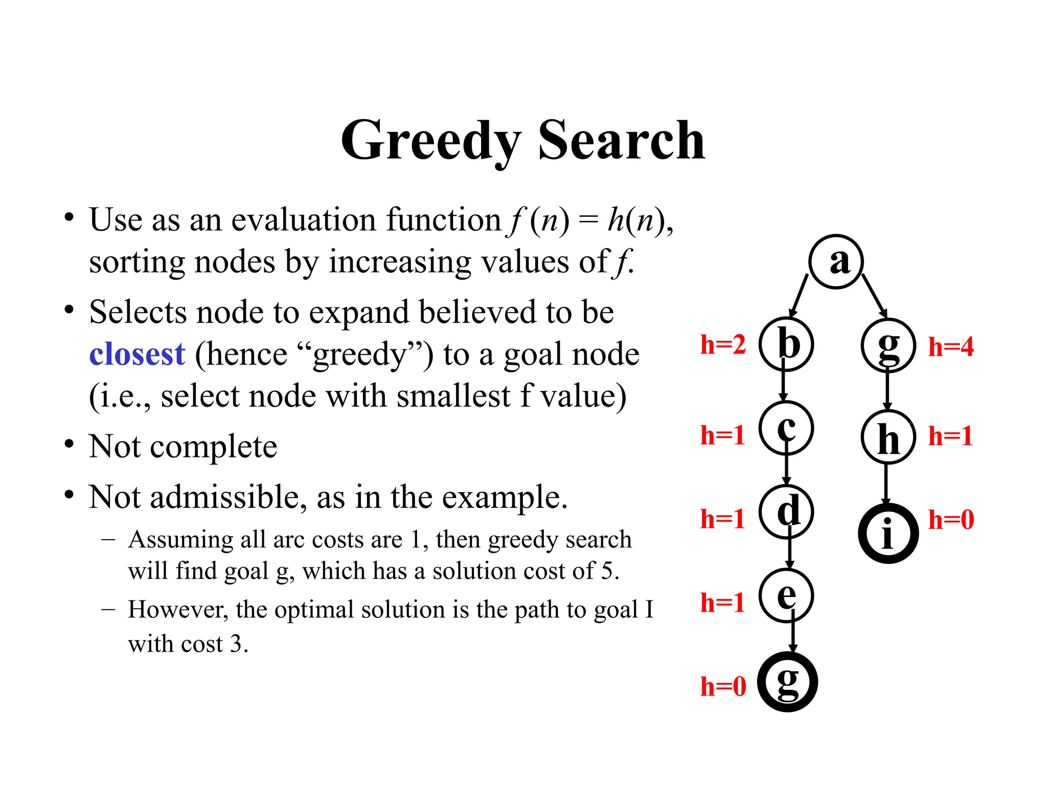
Greedy Search
• Useas an evaluation function f (n) = h(n),
sorting nodes by increasing values of f.
• Selects node to expand believed to be
closest (hence “greedy”) to a goal node
(i.e., select node with smallest f value)
• Not complete
• Not admissible, as in the example.
– Assuming all arc costs are 1, then greedy search
will find goal g, which has a solution cost of 5.
– However, the optimal solution is the path to goal I
with cost 3.
a
g
b
c
d
e
g
h
i
h=2
h=1
h=1
h=1
h=0
h=4
h=1
h=0
21.
Beam Search
• Usean evaluation function f (n) = h(n), but the maximum
size of the nodes list is k, a fixed constant
• Only keeps k best nodes as candidates for expansion, and
throws the rest away
• More space-efficient than greedy search, but may throw
away a node that is on a solution path
• Not complete
• Not admissible
22.
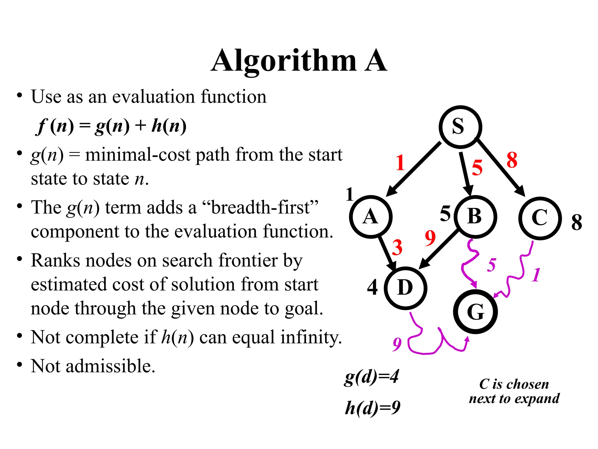
Algorithm A
• Useas an evaluation function
f (n) = g(n) + h(n)
• g(n) = minimal-cost path from the start
state to state n.
• The g(n) term adds a “breadth-first”
component to the evaluation function.
• Ranks nodes on search frontier by
estimated cost of solution from start
node through the given node to goal.
• Not complete if h(n) can equal infinity.
• Not admissible.
S
B
A
D
G
1 5 8
3
1
5
C
1
9
4
5 8
9
g(d)=4
h(d)=9
C is chosen
next to expand
23.
Algorithm A
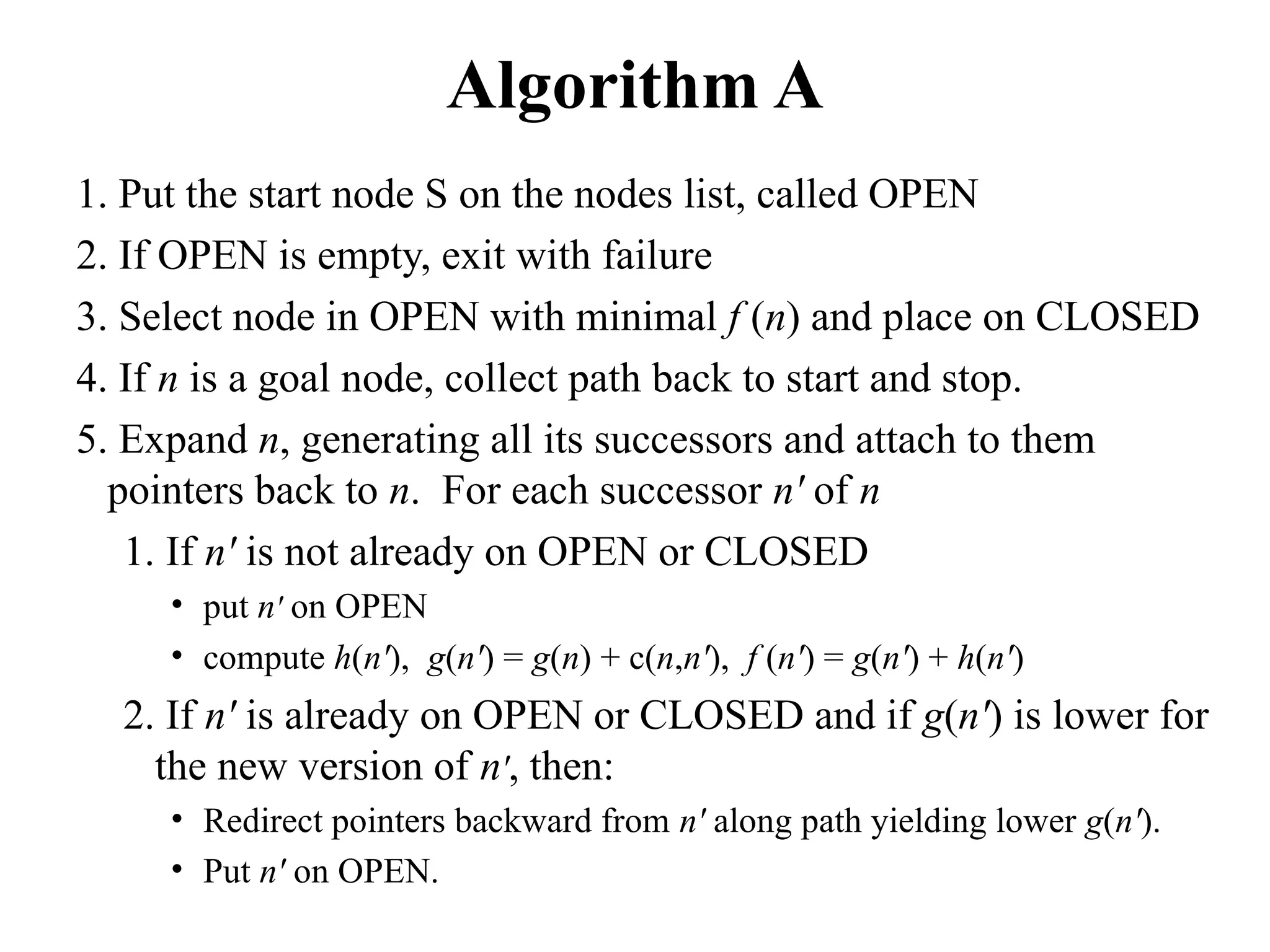
1. Putthe start node S on the nodes list, called OPEN
2. If OPEN is empty, exit with failure
3. Select node in OPEN with minimal f (n) and place on CLOSED
4. If n is a goal node, collect path back to start and stop.
5. Expand n, generating all its successors and attach to them
pointers back to n. For each successor n' of n
1. If n' is not already on OPEN or CLOSED
• put n' on OPEN
• compute h(n'), g(n') = g(n) + c(n,n'), f (n') = g(n') + h(n')
2. If n' is already on OPEN or CLOSED and if g(n') is lower for
the new version of n', then:
• Redirect pointers backward from n' along path yielding lower g(n').
• Put n' on OPEN.
24.
Algorithm A*
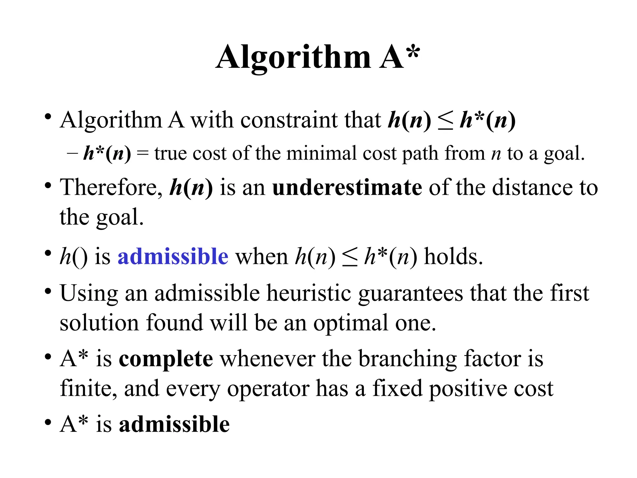
• AlgorithmA with constraint that h(n) ≤ h*(n)
– h*(n) = true cost of the minimal cost path from n to a goal.
• Therefore, h(n) is an underestimate of the distance to
the goal.
• h() is admissible when h(n) ≤ h*(n) holds.
• Using an admissible heuristic guarantees that the first
solution found will be an optimal one.
• A* is complete whenever the branching factor is
finite, and every operator has a fixed positive cost
• A* is admissible
25.
Some Observations onA
• Perfect heuristic: If h(n) = h*(n) for all n, then only the nodes
on the optimal solution path will be expanded. So, no extra work
will be performed.
• Null heuristic: If h(n) = 0 for all n, then this is an admissible
heuristic and A* acts like Uniform-Cost Search.
• Better heuristic: If h1(n) < h2(n) ≤ h*(n) for all non-goal nodes,
then h2 is a better heuristic than h1
– If A1* uses h1, and A2* uses h2, then every node expanded by A2* is also
expanded by A1*.
– In other words, A1 expands at least as many nodes as A2*.
– We say that A2* is better informed than A1*.
• The closer h is to h*, the fewer extra nodes that will be
expanded
26.
Proof of theOptimality of A*
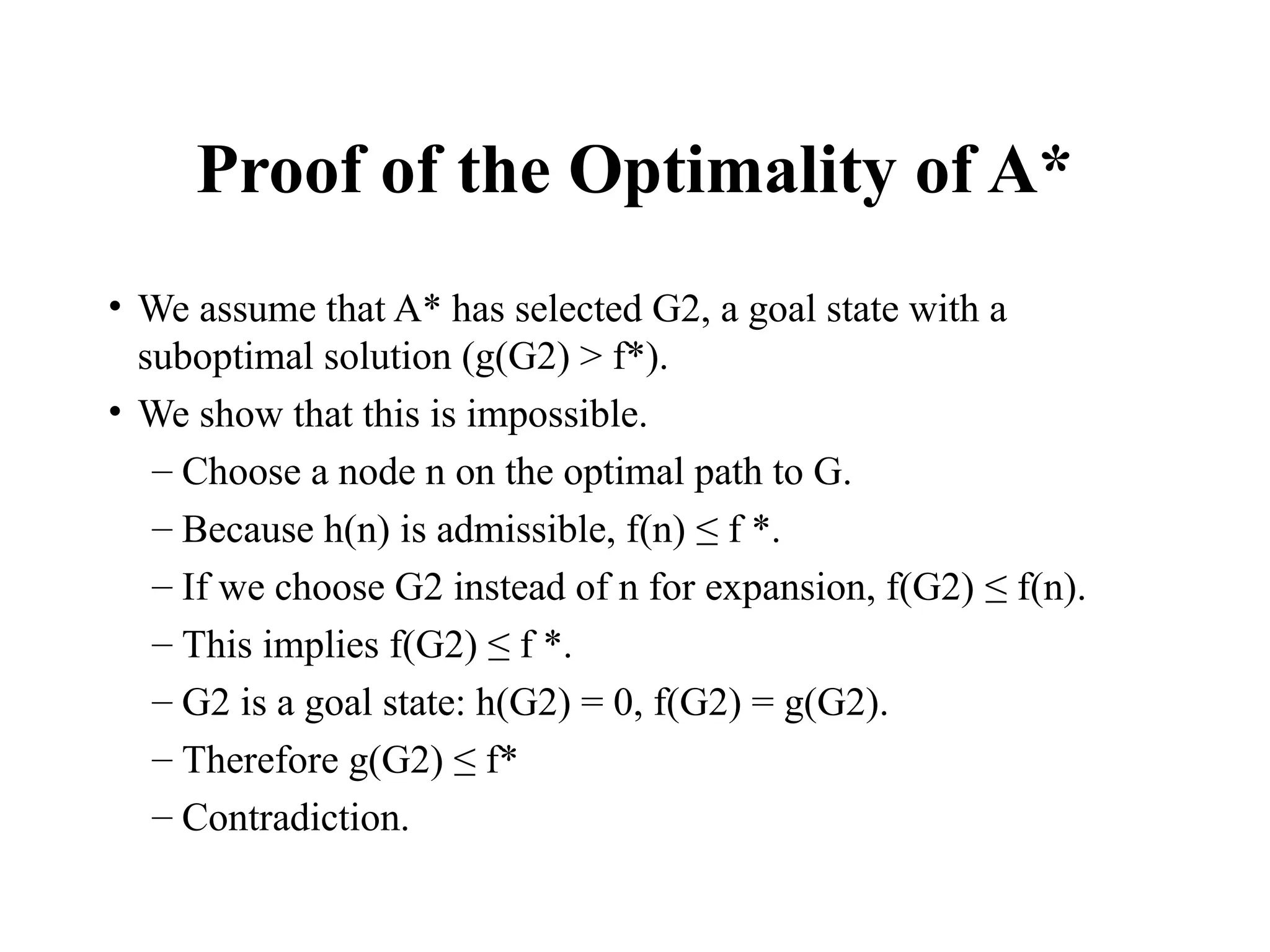
• We assume that A* has selected G2, a goal state with a
suboptimal solution (g(G2) > f*).
• We show that this is impossible.
– Choose a node n on the optimal path to G.
– Because h(n) is admissible, f(n) ≤ f *.
– If we choose G2 instead of n for expansion, f(G2) ≤ f(n).
– This implies f(G2) ≤ f *.
– G2 is a goal state: h(G2) = 0, f(G2) = g(G2).
– Therefore g(G2) ≤ f*
– Contradiction.
27.
Dealing with HardProblems
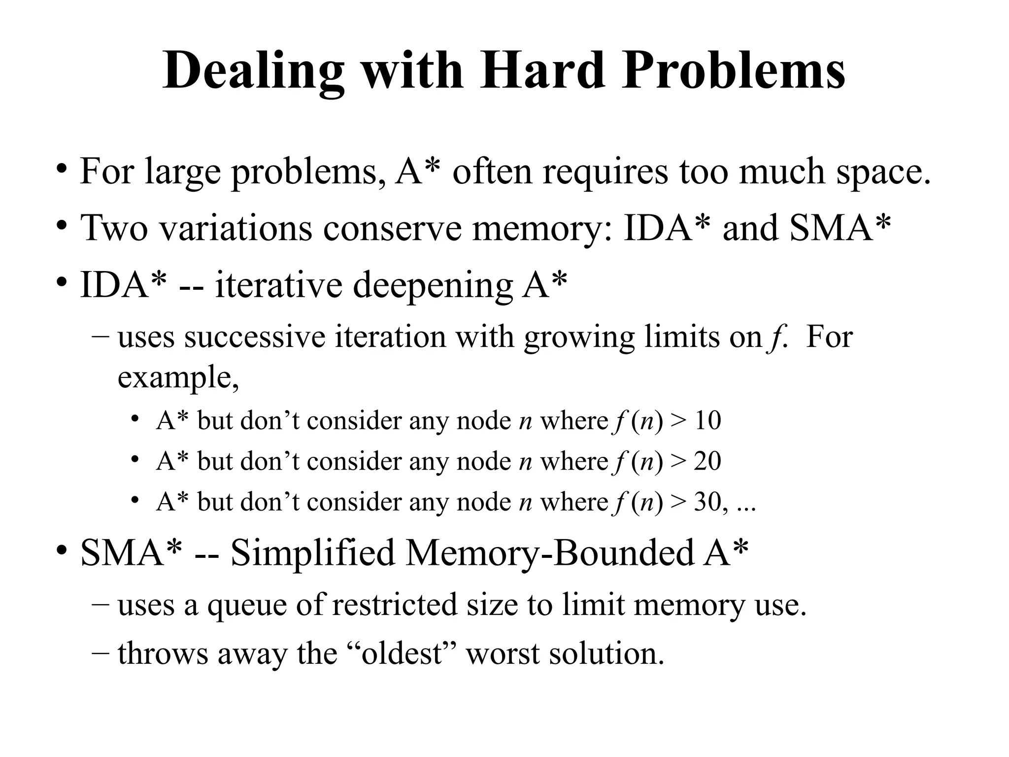
• For large problems, A* often requires too much space.
• Two variations conserve memory: IDA* and SMA*
• IDA* -- iterative deepening A*
– uses successive iteration with growing limits on f. For
example,
• A* but don’t consider any node n where f (n) > 10
• A* but don’t consider any node n where f (n) > 20
• A* but don’t consider any node n where f (n) > 30, ...
• SMA* -- Simplified Memory-Bounded A*
– uses a queue of restricted size to limit memory use.
– throws away the “oldest” worst solution.
28.
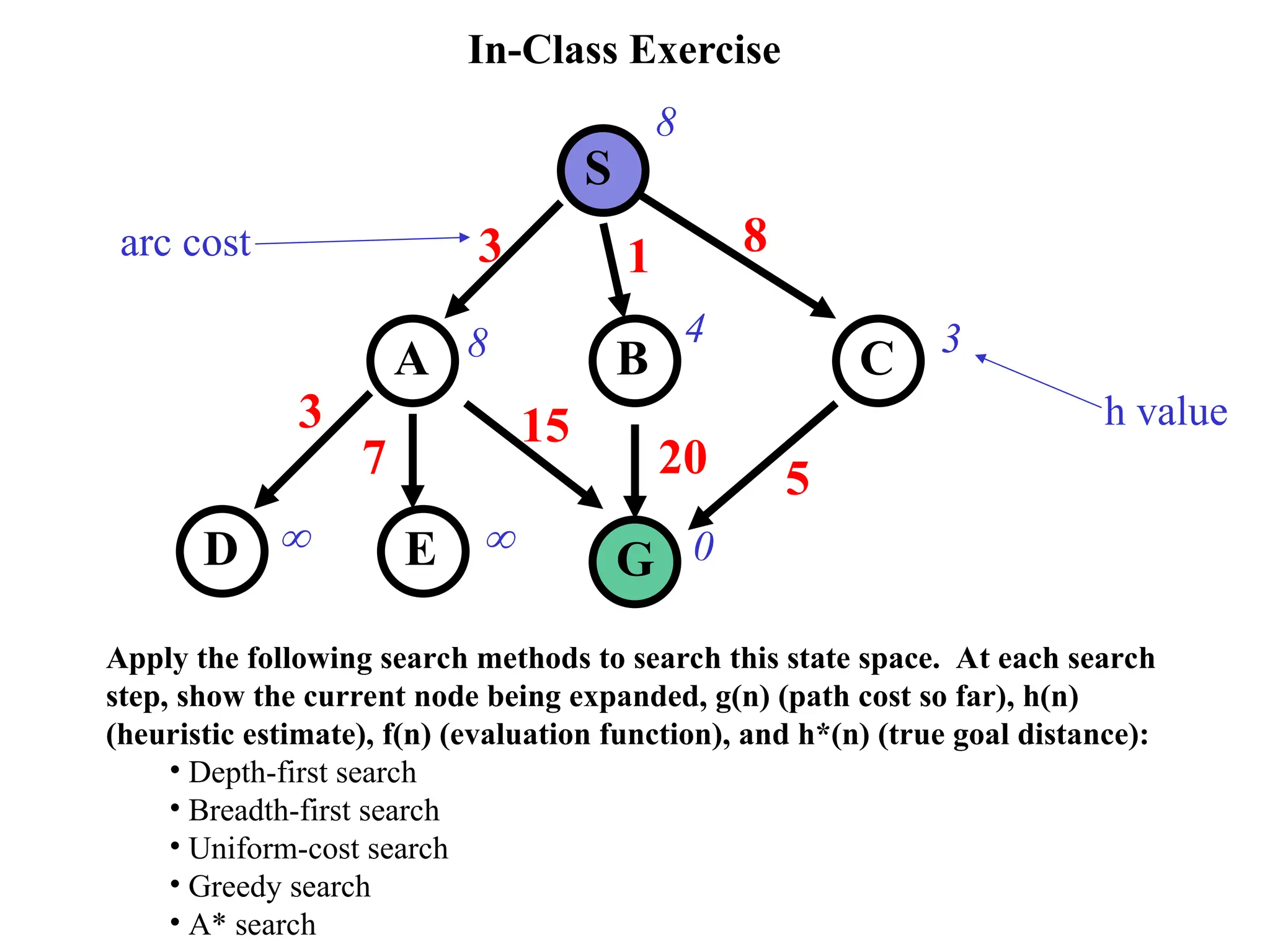
In-Class Exercise
S
C
B
A
D G
E
31 8
15
20 5
3
7
8
8 4 3
0
h value
arc cost
Apply the following search methods to search this state space. At each search
step, show the current node being expanded, g(n) (path cost so far), h(n)
(heuristic estimate), f(n) (evaluation function), and h*(n) (true goal distance):
• Depth-first search
• Breadth-first search
• Uniform-cost search
• Greedy search
• A* search
29.
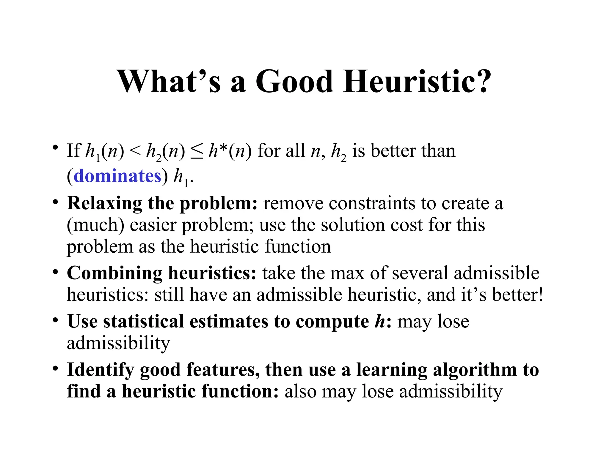
What’s a GoodHeuristic?
• If h1(n) < h2(n) ≤ h*(n) for all n, h2 is better than
(dominates) h1.
• Relaxing the problem: remove constraints to create a
(much) easier problem; use the solution cost for this
problem as the heuristic function
• Combining heuristics: take the max of several admissible
heuristics: still have an admissible heuristic, and it’s better!
• Use statistical estimates to compute h: may lose
admissibility
• Identify good features, then use a learning algorithm to
find a heuristic function: also may lose admissibility
30.
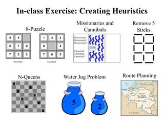
In-class Exercise: CreatingHeuristics
8-Puzzle
N-Queens
Missionaries and
Cannibals
Remove 5
Sticks
Water Jug Problem
5
2
Route Planning
31.
Summary: Informed Search
•Best-first search is general search where the minimum-cost nodes (according
to some measure) are expanded first.
• Greedy search uses minimal estimated cost h(n) to the goal state as measure.
This reduces the search time, but the algorithm is neither complete nor optimal.
• A* search combines uniform-cost search and greedy search: f (n) = g(n) +
h(n). A* handles state repetitions and h(n) never overestimates.
– A* is complete and optimal, but space complexity is high.
– The time complexity depends on the quality of the heuristic function.
– IDA* and SMA* reduce the memory requirements of A*.