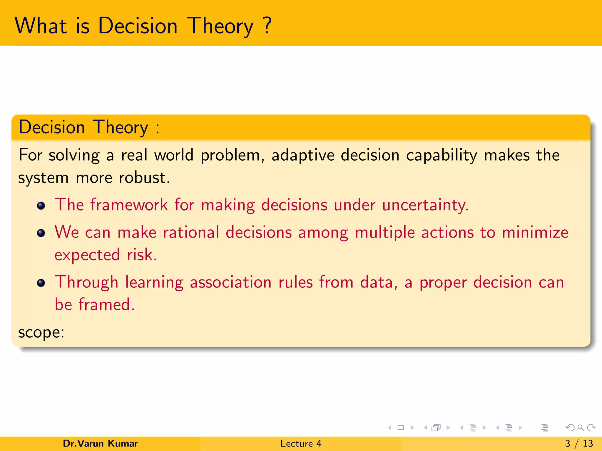
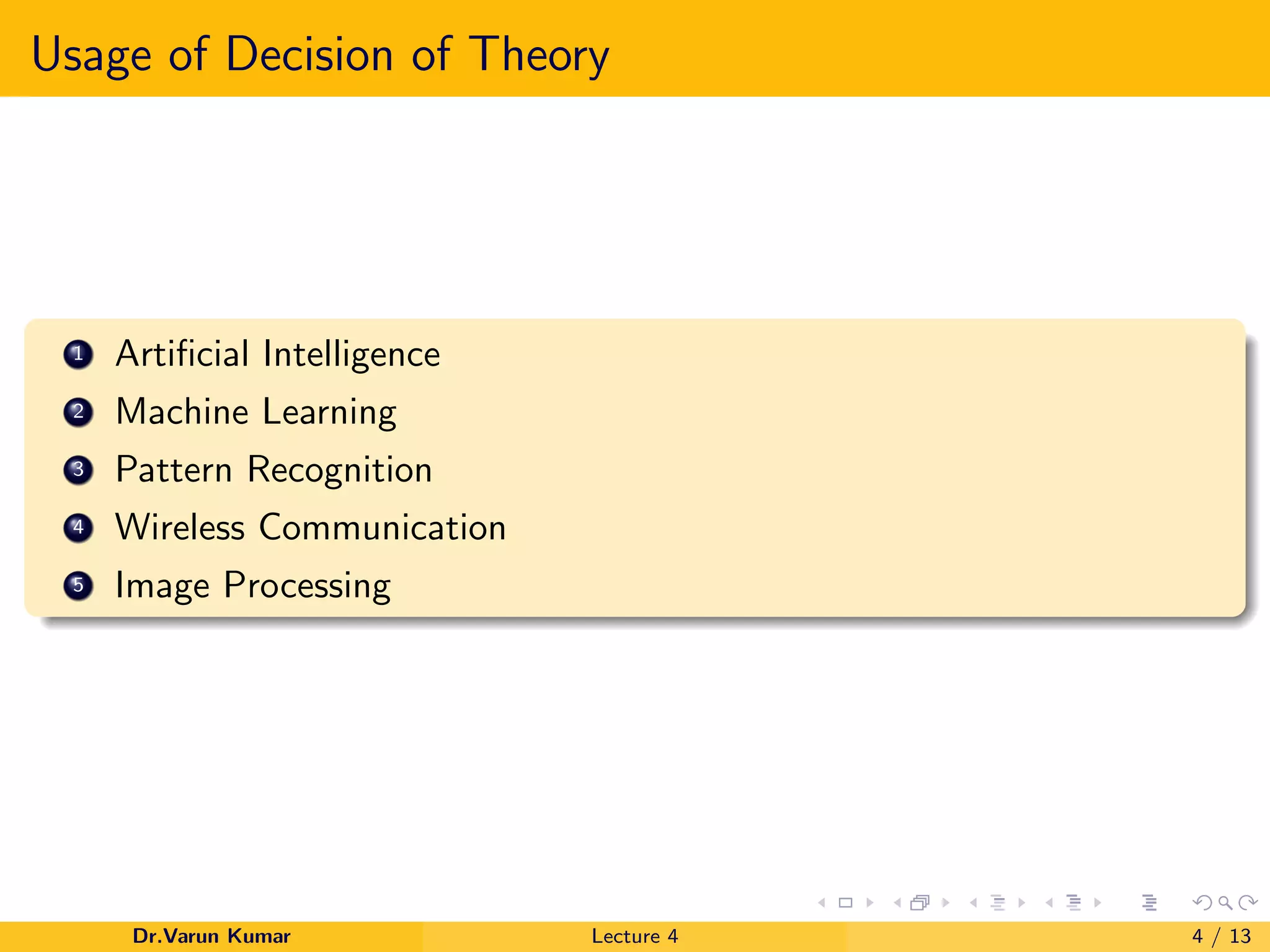
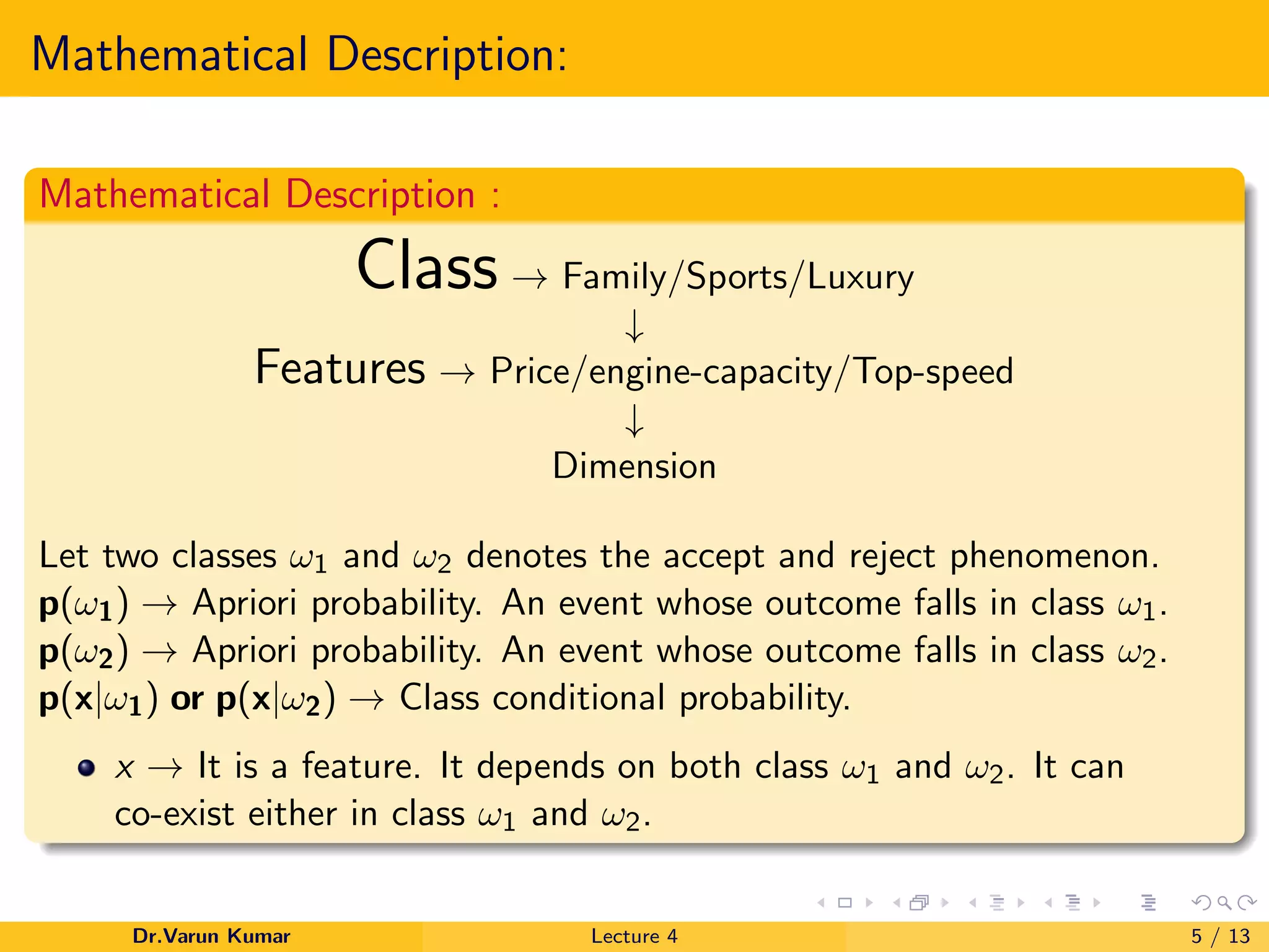
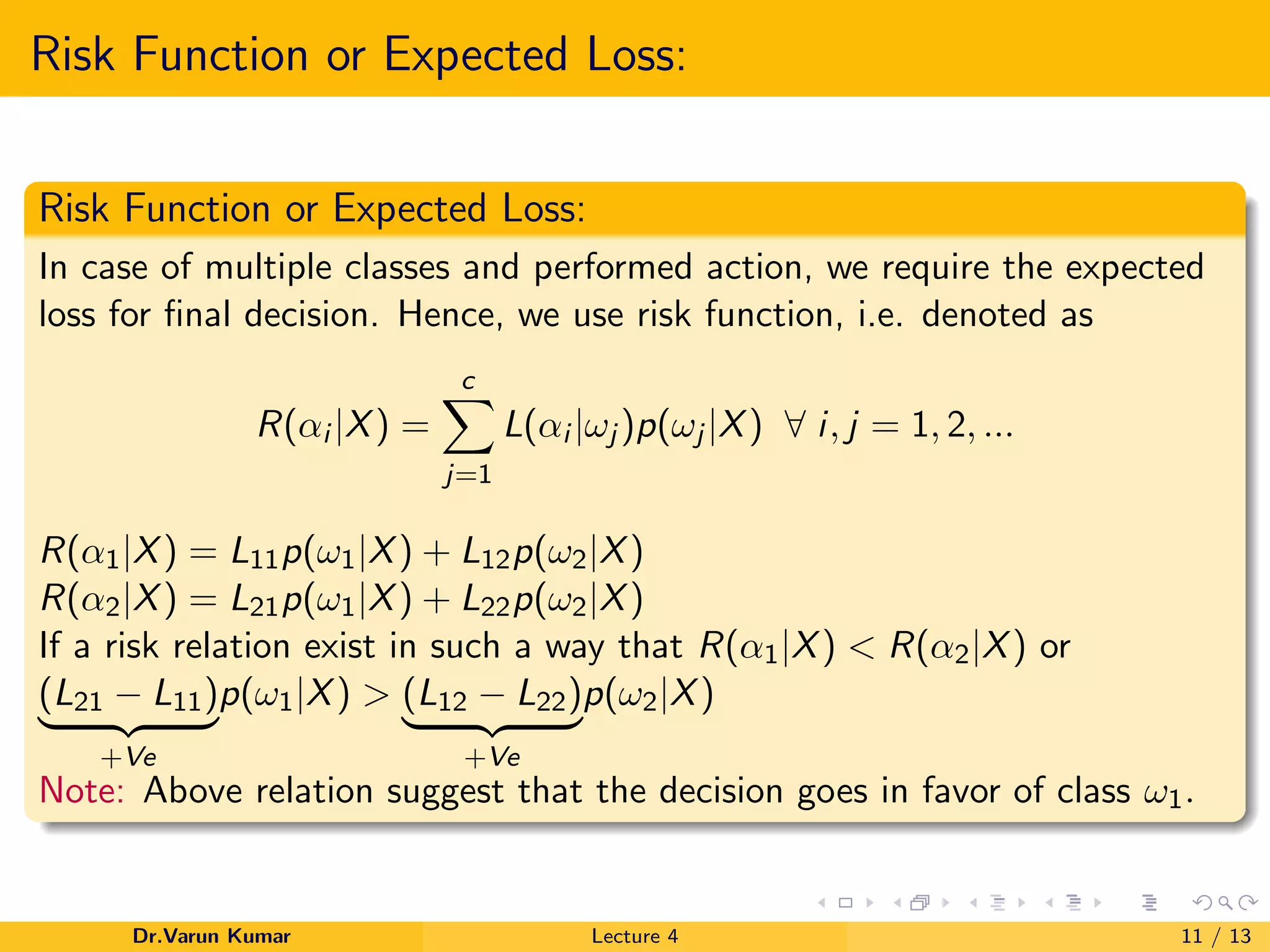
KEMBAR78
Bayesian decesion theory | PDF
Bayesian Decision Theory
Dr.Varun Kumar
Dr.Varun Kumar Lecture 4 1 / 13
Outlines
1 What is Decision Theory ?
2 Usage of Decision of Theory
3 Mathematical Description of Baye’s Theorem:
4 References
Dr.Varun Kumar Lecture 4 2 / 13
What is Decision Theory ?
Decision Theory :
For solving a real world problem, adaptive decision capability makes the
system more robust.
The framework for making decisions under uncertainty.
We can make rational decisions among multiple actions to minimize
expected risk.
Through learning association rules from data, a proper decision can
be framed.
scope:
Dr.Varun Kumar Lecture 4 3 / 13
Usage of Decision of Theory
1 Artificial Intelligence
2 Machine Learning
3 Pattern Recognition
4 Wireless Communication
5 Image Processing
Dr.Varun Kumar Lecture 4 4 / 13
Mathematical Description:
Mathematical Description :
Class → Family/Sports/Luxury
↓
Features → Price/engine-capacity/Top-speed
↓
Dimension
Let two classes ω1 and ω2 denotes the accept and reject phenomenon.
p(ω1) → Apriori probability. An event whose outcome falls in class ω1.
p(ω2) → Apriori probability. An event whose outcome falls in class ω2.
p(x|ω1) or p(x|ω2) → Class conditional probability.
x → It is a feature. It depends on both class ω1 and ω2. It can
co-exist either in class ω1 and ω2.
Dr.Varun Kumar Lecture 4 5 / 13
Continued–
Mathematical Description:
p(ω1|x) → Aposteriori probability (depends on current input or future).
p(ωi , x) ∀ i = 1, 2 → Joint probability
Joint Probability:
p(ωi , x) = p(ωi |x)p(x) = p(x|ωi )p(ωi )
Property of Joint probability:
p(x) = 2
i=1 p(ωi , x)
p(ωi |x) =
p(x|ωi )p(ωi )
p(x)
=
p(x|ωi )p(ωi )
2
i=1 p(ωi , x)
p(ω1|x) > p(ω2|x) ⇒ Decision will go in favor of class ω1.
p(ω1|x) < p(ω2|x) ⇒ Decision will go in favor of class ω2.
Note: Aposteriori probability gives the true measure of any new sample
that may fall in the class ω1 and ω2.
Dr.Varun Kumar Lecture 4 6 / 13
Continued–
Note:
1 If the relation between apriori probability is p(ω1) > p(ω2) ⇒
Decision goes in favor of class ω1. This phenomenon is less likely.
2 Above relation does not address the actual scenario of the condition
of class ω1 and ω2.
3 On the other side, if the relation between aposteriori probability is
p(ω1|x) > p(ω2|x) ⇒ decision will go in favor of class ω1. This
phenomenon is more likely.
4 Random variable x is function of ω1 and ω2.
x = f (ω1, ω2)
Dr.Varun Kumar Lecture 4 7 / 13
Probability of Error:
0 2 4 6 8 10 12
x
0
0.05
0.1
0.15
0.2
0.25
0.3
0.35
0.4
p(ωi
|x)
ω1
ω2
x1
x0
x2
p(ω1
|x0
) = p(ω2
|xo
)
p(ω1
|x1
) > p(ω2
|x1
)
p(ω1
|x2
) < p(ω2
|x2
)
p(error) =
∞
−∞
p(error, x)dx =
∞
−∞
p(error|x)p(x)dx
where, p(error|x) = min{p(ω1|x), p(ω2|x)}
Dr.Varun Kumar Lecture 4 8 / 13
Example
Q. If a feature x is the essential part of two classes ω1 and ω2. If the
PDF of this feature is exponentially distributed, such that
p(x) = 1
2e−x/2 ∀ x > 0 and aposteriori PDF for ω1 and ω2 are
2e−2x ∀ x > 0 and 4e−4x ∀ x > 0, respectively.
1 Find the probability of error, when decision goes in favor of ω1.
2 Find the probability of error, when decision goes in favor of ω2.
3 At what value of feature x, the decision can’t be performed.
Ans. 1 According to question, p(x) = 1
2 e−x/2
∀ x > 0,
p(ω1|x) = 2e−2x
∀ x > 0 and p(ω2|x) = 4e−4x
∀ x > 0 . If decision
goes in favor of ω1 then p(error/x) = p(ω2/x).
p(error)|ω1 =
∞
0
4e−4x 1
2 e−x/2
dx=4
9 ∀ x > 0
2 p(error)|ω2 =
∞
0
2e−2x 1
2 e−x/2
dx=2
5 ∀ x > 0
3 when aposteriori PDF for class ω1 and ω2 are same,i.e
2e−2x
= 4e−4x
⇒ e2x
= 2 ⇒ x = 1
2 ln(2)
Dr.Varun Kumar Lecture 4 9 / 13
Multiple Class, Loss Function:
Multiple Class/Actions/Features and Loss Function:
{ω1, ω2, ...., ωc} ⇒ Multiple class or state of nature
{α1, α2, ...., αa} ⇒ Multiple actions
Loss Function:
Instead of probability of error, we use the term loss function in case of
multiple classes and actions. Mathematically, it can be expressed as
L(αi /ωj ) = Lij ⇒ A given action i is performed under jth
state of nature
∀ i = 1, 2, ...a and j = 1, 2, ..., c
X → d-dimensional feature vector, i.e. X = {x1, x2, ....xd }
Dr.Varun Kumar Lecture 4 10 / 13
Risk Function or Expected Loss:
In case of multiple classes and performed action, we require the expected
loss for final decision. Hence, we use risk function, i.e. denoted as
R(αi |X) =
c
j=1
L(αi |ωj )p(ωj |X) ∀ i, j = 1, 2, ...
R(α1|X) = L11p(ω1|X) + L12p(ω2|X)
R(α2|X) = L21p(ω1|X) + L22p(ω2|X)
If a risk relation exist in such a way that R(α1|X) < R(α2|X) or
(L21 − L11)
+Ve
p(ω1|X) > (L12 − L22)
+Ve
p(ω2|X)
Note: Above relation suggest that the decision goes in favor of class ω1.
Dr.Varun Kumar Lecture 4 11 / 13
Minimum Error Rate Classification
L(αi |ωj ) = 0 ∀ i = j ⇒ No loss occur for performing the ith action
correspond to ith class
= 1 ∀ i = j
Risk Function :
R(αi |X) = c
j=i p(ωj |X) = 1 − p(ωi |X)
Dr.Varun Kumar Lecture 4 12 / 13
References
E. Alpaydin, Introduction to machine learning. MIT press, 2020.
T. M. Mitchell, The discipline of machine learning. Carnegie Mellon University,
School of Computer Science, Machine Learning , 2006, vol. 9.
J. Grus, Data science from scratch: first principles with python. O’Reilly Media,
2019.
Dr.Varun Kumar Lecture 4 13 / 13

Bayesian decesion theory

  • 1.
    Bayesian Decision Theory Dr.VarunKumar Dr.Varun Kumar Lecture 4 1 / 13
  • 2.
    Outlines 1 What isDecision Theory ? 2 Usage of Decision of Theory 3 Mathematical Description of Baye’s Theorem: 4 References Dr.Varun Kumar Lecture 4 2 / 13
  • 3.
    What is DecisionTheory ? Decision Theory : For solving a real world problem, adaptive decision capability makes the system more robust. The framework for making decisions under uncertainty. We can make rational decisions among multiple actions to minimize expected risk. Through learning association rules from data, a proper decision can be framed. scope: Dr.Varun Kumar Lecture 4 3 / 13
  • 4.
    Usage of Decisionof Theory 1 Artificial Intelligence 2 Machine Learning 3 Pattern Recognition 4 Wireless Communication 5 Image Processing Dr.Varun Kumar Lecture 4 4 / 13
  • 5.
    Mathematical Description: Mathematical Description: Class → Family/Sports/Luxury ↓ Features → Price/engine-capacity/Top-speed ↓ Dimension Let two classes ω1 and ω2 denotes the accept and reject phenomenon. p(ω1) → Apriori probability. An event whose outcome falls in class ω1. p(ω2) → Apriori probability. An event whose outcome falls in class ω2. p(x|ω1) or p(x|ω2) → Class conditional probability. x → It is a feature. It depends on both class ω1 and ω2. It can co-exist either in class ω1 and ω2. Dr.Varun Kumar Lecture 4 5 / 13
  • 6.
    Continued– Mathematical Description: p(ω1|x) →Aposteriori probability (depends on current input or future). p(ωi , x) ∀ i = 1, 2 → Joint probability Joint Probability: p(ωi , x) = p(ωi |x)p(x) = p(x|ωi )p(ωi ) Property of Joint probability: p(x) = 2 i=1 p(ωi , x) p(ωi |x) = p(x|ωi )p(ωi ) p(x) = p(x|ωi )p(ωi ) 2 i=1 p(ωi , x) p(ω1|x) > p(ω2|x) ⇒ Decision will go in favor of class ω1. p(ω1|x) < p(ω2|x) ⇒ Decision will go in favor of class ω2. Note: Aposteriori probability gives the true measure of any new sample that may fall in the class ω1 and ω2. Dr.Varun Kumar Lecture 4 6 / 13
  • 7.
    Continued– Note: 1 If therelation between apriori probability is p(ω1) > p(ω2) ⇒ Decision goes in favor of class ω1. This phenomenon is less likely. 2 Above relation does not address the actual scenario of the condition of class ω1 and ω2. 3 On the other side, if the relation between aposteriori probability is p(ω1|x) > p(ω2|x) ⇒ decision will go in favor of class ω1. This phenomenon is more likely. 4 Random variable x is function of ω1 and ω2. x = f (ω1, ω2) Dr.Varun Kumar Lecture 4 7 / 13
  • 8.
    Probability of Error: Probabilityof Error: 0 2 4 6 8 10 12 x 0 0.05 0.1 0.15 0.2 0.25 0.3 0.35 0.4 p(ωi |x) ω1 ω2 x1 x0 x2 p(ω1 |x0 ) = p(ω2 |xo ) p(ω1 |x1 ) > p(ω2 |x1 ) p(ω1 |x2 ) < p(ω2 |x2 ) p(error) = ∞ −∞ p(error, x)dx = ∞ −∞ p(error|x)p(x)dx where, p(error|x) = min{p(ω1|x), p(ω2|x)} Dr.Varun Kumar Lecture 4 8 / 13
  • 9.
    Example Q. If afeature x is the essential part of two classes ω1 and ω2. If the PDF of this feature is exponentially distributed, such that p(x) = 1 2e−x/2 ∀ x > 0 and aposteriori PDF for ω1 and ω2 are 2e−2x ∀ x > 0 and 4e−4x ∀ x > 0, respectively. 1 Find the probability of error, when decision goes in favor of ω1. 2 Find the probability of error, when decision goes in favor of ω2. 3 At what value of feature x, the decision can’t be performed. Ans. 1 According to question, p(x) = 1 2 e−x/2 ∀ x > 0, p(ω1|x) = 2e−2x ∀ x > 0 and p(ω2|x) = 4e−4x ∀ x > 0 . If decision goes in favor of ω1 then p(error/x) = p(ω2/x). p(error)|ω1 = ∞ 0 4e−4x 1 2 e−x/2 dx=4 9 ∀ x > 0 2 p(error)|ω2 = ∞ 0 2e−2x 1 2 e−x/2 dx=2 5 ∀ x > 0 3 when aposteriori PDF for class ω1 and ω2 are same,i.e 2e−2x = 4e−4x ⇒ e2x = 2 ⇒ x = 1 2 ln(2) Dr.Varun Kumar Lecture 4 9 / 13
  • 10.
    Multiple Class, LossFunction: Multiple Class/Actions/Features and Loss Function: {ω1, ω2, ...., ωc} ⇒ Multiple class or state of nature {α1, α2, ...., αa} ⇒ Multiple actions Loss Function: Instead of probability of error, we use the term loss function in case of multiple classes and actions. Mathematically, it can be expressed as L(αi /ωj ) = Lij ⇒ A given action i is performed under jth state of nature ∀ i = 1, 2, ...a and j = 1, 2, ..., c X → d-dimensional feature vector, i.e. X = {x1, x2, ....xd } Dr.Varun Kumar Lecture 4 10 / 13
  • 11.
    Risk Function orExpected Loss: Risk Function or Expected Loss: In case of multiple classes and performed action, we require the expected loss for final decision. Hence, we use risk function, i.e. denoted as R(αi |X) = c j=1 L(αi |ωj )p(ωj |X) ∀ i, j = 1, 2, ... R(α1|X) = L11p(ω1|X) + L12p(ω2|X) R(α2|X) = L21p(ω1|X) + L22p(ω2|X) If a risk relation exist in such a way that R(α1|X) < R(α2|X) or (L21 − L11) +Ve p(ω1|X) > (L12 − L22) +Ve p(ω2|X) Note: Above relation suggest that the decision goes in favor of class ω1. Dr.Varun Kumar Lecture 4 11 / 13
  • 12.
    Minimum Error RateClassification L(αi |ωj ) = 0 ∀ i = j ⇒ No loss occur for performing the ith action correspond to ith class = 1 ∀ i = j Risk Function : R(αi |X) = c j=i p(ωj |X) = 1 − p(ωi |X) Dr.Varun Kumar Lecture 4 12 / 13
  • 13.
    References E. Alpaydin, Introductionto machine learning. MIT press, 2020. T. M. Mitchell, The discipline of machine learning. Carnegie Mellon University, School of Computer Science, Machine Learning , 2006, vol. 9. J. Grus, Data science from scratch: first principles with python. O’Reilly Media, 2019. Dr.Varun Kumar Lecture 4 13 / 13