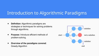
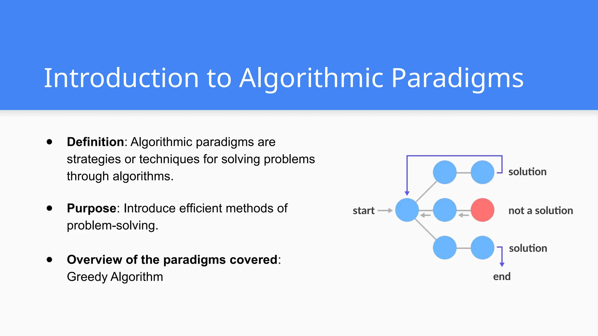
Introduction to AlgorithmicParadigms
● Definition: Algorithmic paradigms are
strategies or techniques for solving problems
through algorithms.
● Purpose: Introduce efficient methods of
problem-solving.
● Overview of the paradigms covered:
Greedy Algorithm
3.
What is Backtracking?
Definition:Backtracking is a general algorithmic technique that searches for solutions by trying to build a solution
incrementally and abandoning partial solutions that fail to meet the criteria.
Key Points:
● Solves constraint satisfaction problems.
● Uses recursion.
● Explores all possible solutions.
Example Problem: Sudoku, N-Queens problem
4.
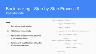
Backtracking - Step-by-StepProcess &
Pseudocode
Steps:
1. Start with an empty solution.
2. Add choices incrementally.
3. If the current choice is invalid, backtrack
to the previous choice.
4. Continue until a valid solution is found or
all choices are explored.
def backtrack(state):
if is_solution(state):
return state
for option in possible_choices(state):
if is_valid(option):
result =
backtrack(new_state(option))
if result is not None:
return result
return None
5.
What is Branch-and-Bound?
Definition:Branch-and-Bound is a paradigm used for solving optimization problems by systematically
exploring the solution space and pruning branches that do not lead to an optimal solution.
Key Points:
● Focus on finding optimal solutions.
● Uses bounds to eliminate suboptimal solutions.
● Common in combinatorial optimization problems.
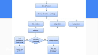
Backtracking - Step-by-StepProcess
Steps:
1. Calculate an upper or lower bound for the solution.
2. Partition the problem into subproblems (branches).
3. Explore the branches while keeping track of the best
solution found.
4. Prune branches that cannot produce a better solution
than the best found.
5. .
Pseudocode Example:
def branch_and_bound(problem):
best_solution = None
queue = [initial_state]
while queue:
node = queue.pop()
if is_better_than(best_solution,
node):
best_solution = node
for branch in branches(node):
if bound(branch) < best_solution:
queue.append(branch)
return best_solution
8.
Backtracking vs Branch-and-Bound
●Key Differences:
○ Objective: Backtracking searches all solutions; Branch-and-Bound focuses on optimization.
○ Solution type: Backtracking often works on constraint satisfaction; Branch-and-Bound works on
optimization problems.
○ Pruning: Branch-and-Bound uses bounding to prune branches, while backtracking uses a trial-and-error
approach.
9.
Backtracking - UseCase:
Job Scheduling in Cloud Computing
Problem: In a cloud environment, jobs need to be assigned to servers without overloading any server’s capacity (in terms
of CPU, memory, etc.).
Backtracking Approach:
1. Start with an empty assignment of jobs.
2. Add jobs incrementally, ensuring that no server exceeds capacity.
3. If capacity is exceeded, backtrack and try a different assignment.
4. Continue until all jobs are successfully assigned.
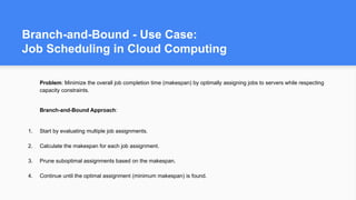
10.
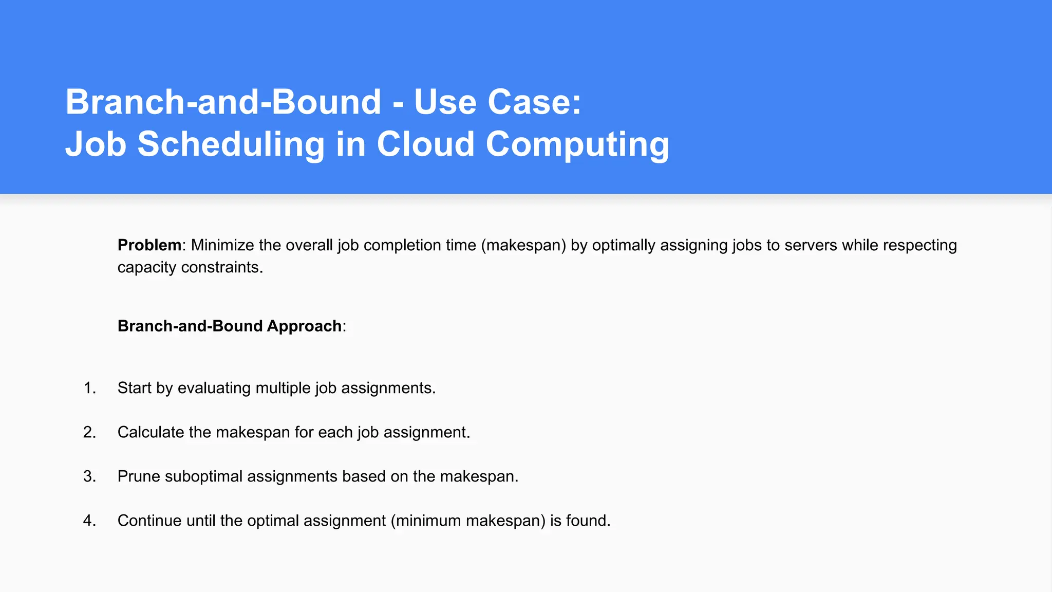
Branch-and-Bound - UseCase:
Job Scheduling in Cloud Computing
Problem: Minimize the overall job completion time (makespan) by optimally assigning jobs to servers while respecting
capacity constraints.
Branch-and-Bound Approach:
1. Start by evaluating multiple job assignments.
2. Calculate the makespan for each job assignment.
3. Prune suboptimal assignments based on the makespan.
4. Continue until the optimal assignment (minimum makespan) is found.
11.
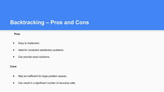
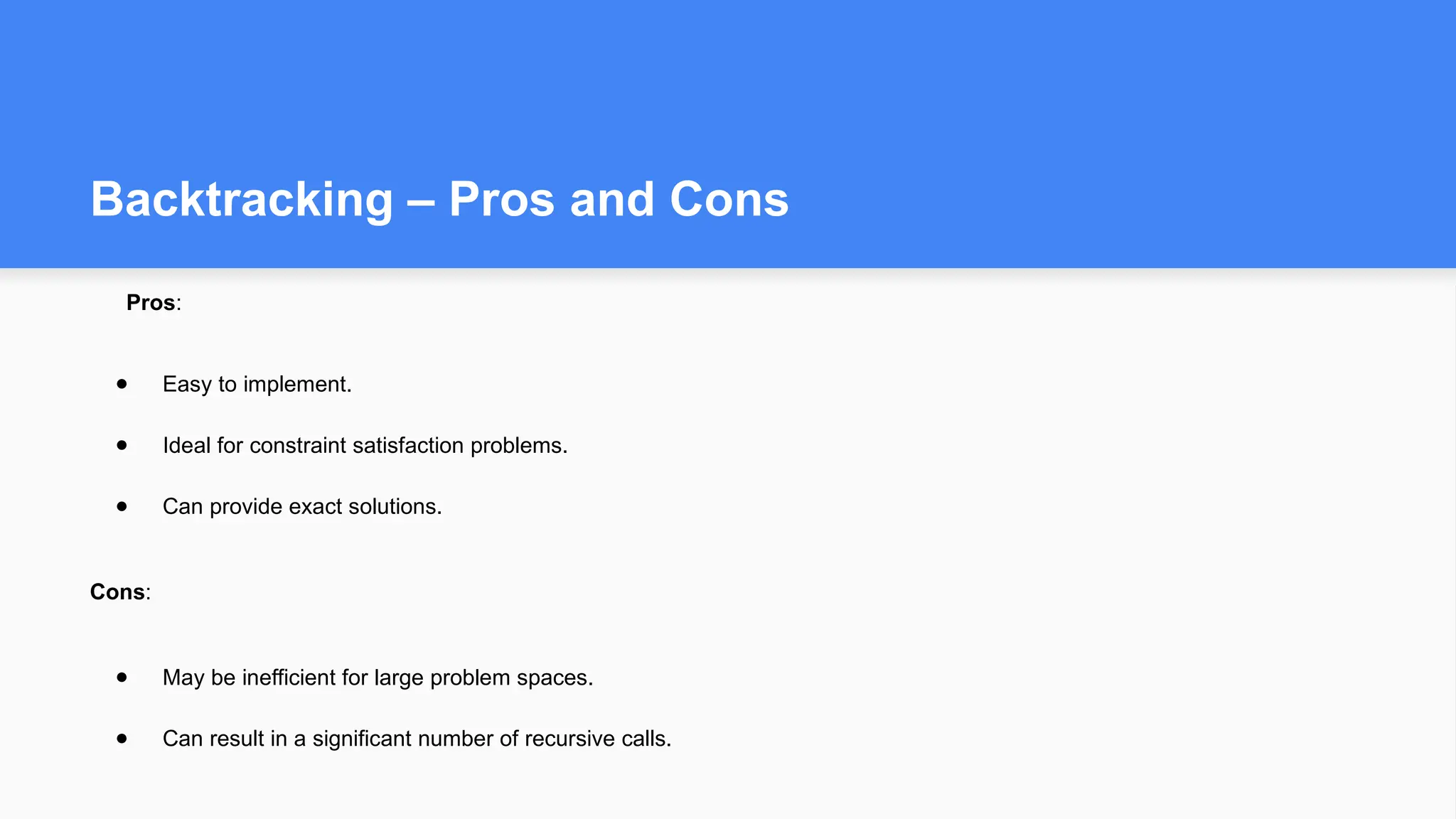
Backtracking – Prosand Cons
Pros:
● Easy to implement.
● Ideal for constraint satisfaction problems.
● Can provide exact solutions.
Cons:
● May be inefficient for large problem spaces.
● Can result in a significant number of recursive calls.
12.
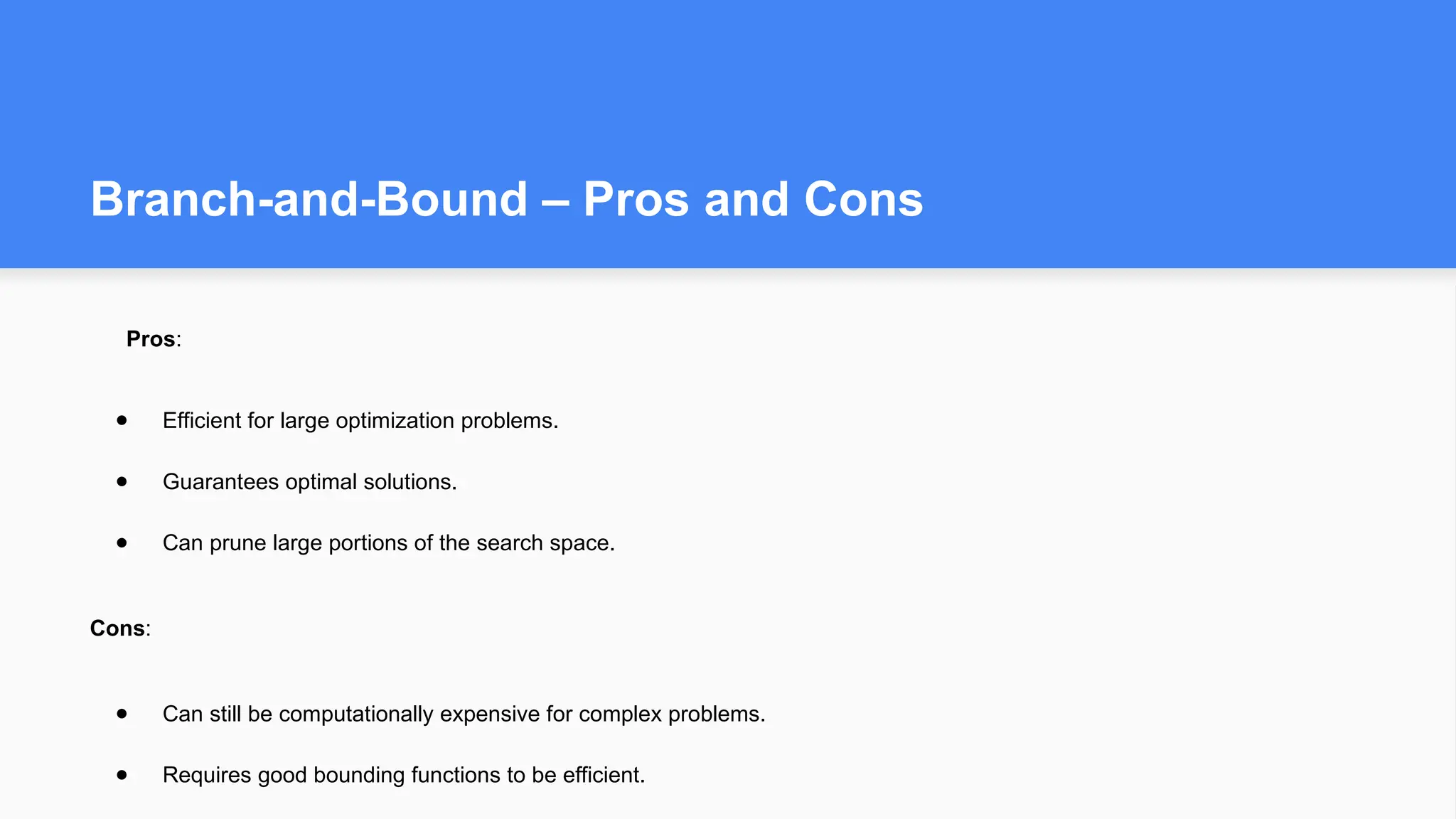
Branch-and-Bound – Prosand Cons
Pros:
● Efficient for large optimization problems.
● Guarantees optimal solutions.
● Can prune large portions of the search space.
Cons:
● Can still be computationally expensive for complex problems.
● Requires good bounding functions to be efficient.
13.
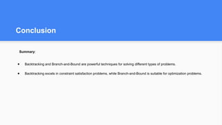
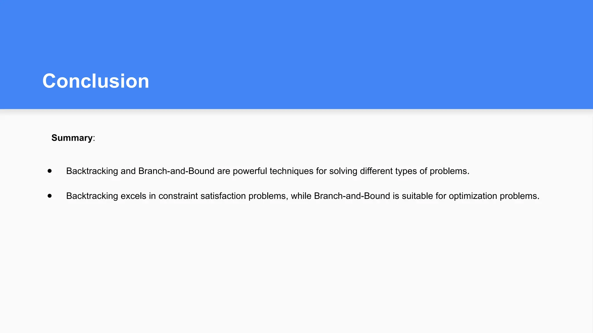
Conclusion
Summary:
● Backtracking andBranch-and-Bound are powerful techniques for solving different types of problems.
● Backtracking excels in constraint satisfaction problems, while Branch-and-Bound is suitable for optimization problems.


![Backtracking - Step-by-Step Process
Steps:
1. Calculate an upper or lower bound for the solution.
2. Partition the problem into subproblems (branches).
3. Explore the branches while keeping track of the best
solution found.
4. Prune branches that cannot produce a better solution
than the best found.
5. .
Pseudocode Example:
def branch_and_bound(problem):
best_solution = None
queue = [initial_state]
while queue:
node = queue.pop()
if is_better_than(best_solution,
node):
best_solution = node
for branch in branches(node):
if bound(branch) < best_solution:
queue.append(branch)
return best_solution](https://image.slidesharecdn.com/mayureshvirkardatastructuresassignment-250703141634-08181f30/85/Branch-and-Bound-Algorithm-presentation-paradigm-7-320.jpg)


![Backtracking - Step-by-Step Process
Steps:
1. Calculate an upper or lower bound for the solution.
2. Partition the problem into subproblems (branches).
3. Explore the branches while keeping track of the best
solution found.
4. Prune branches that cannot produce a better solution
than the best found.
5. .
Pseudocode Example:
def branch_and_bound(problem):
best_solution = None
queue = [initial_state]
while queue:
node = queue.pop()
if is_better_than(best_solution,
node):
best_solution = node
for branch in branches(node):
if bound(branch) < best_solution:
queue.append(branch)
return best_solution](https://image.slidesharecdn.com/mayureshvirkardatastructuresassignment-250703141634-08181f30/75/Branch-and-Bound-Algorithm-presentation-paradigm-7-2048.jpg)


![BranchandBoundAlgorithms[1].ppt](https://cdn.slidesharecdn.com/ss_thumbnails/branchandboundalgorithms1-230104091253-13fa4911-thumbnail.jpg?width=600ounds&width=560&fit=bounds)


