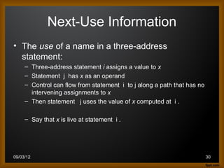
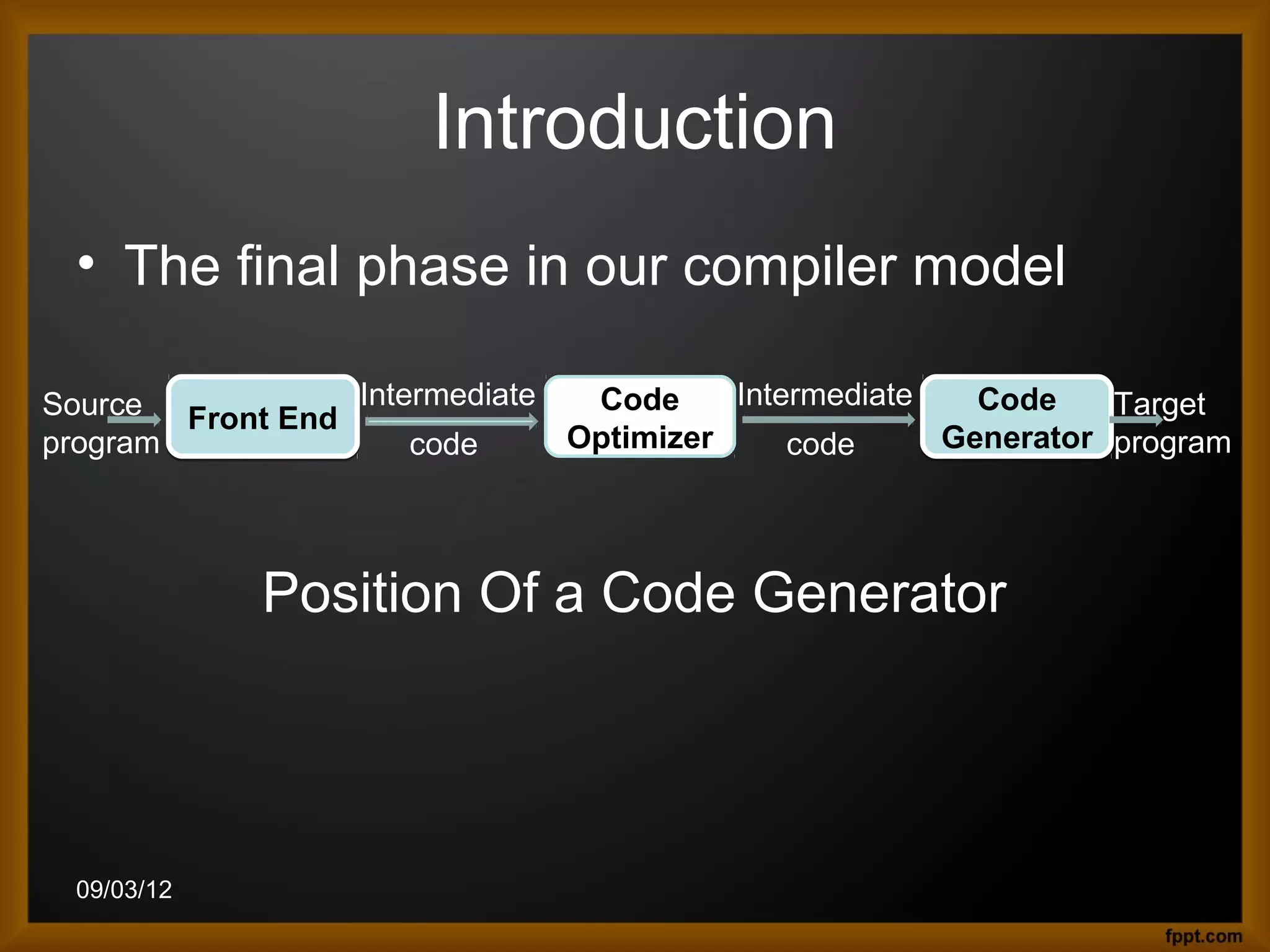
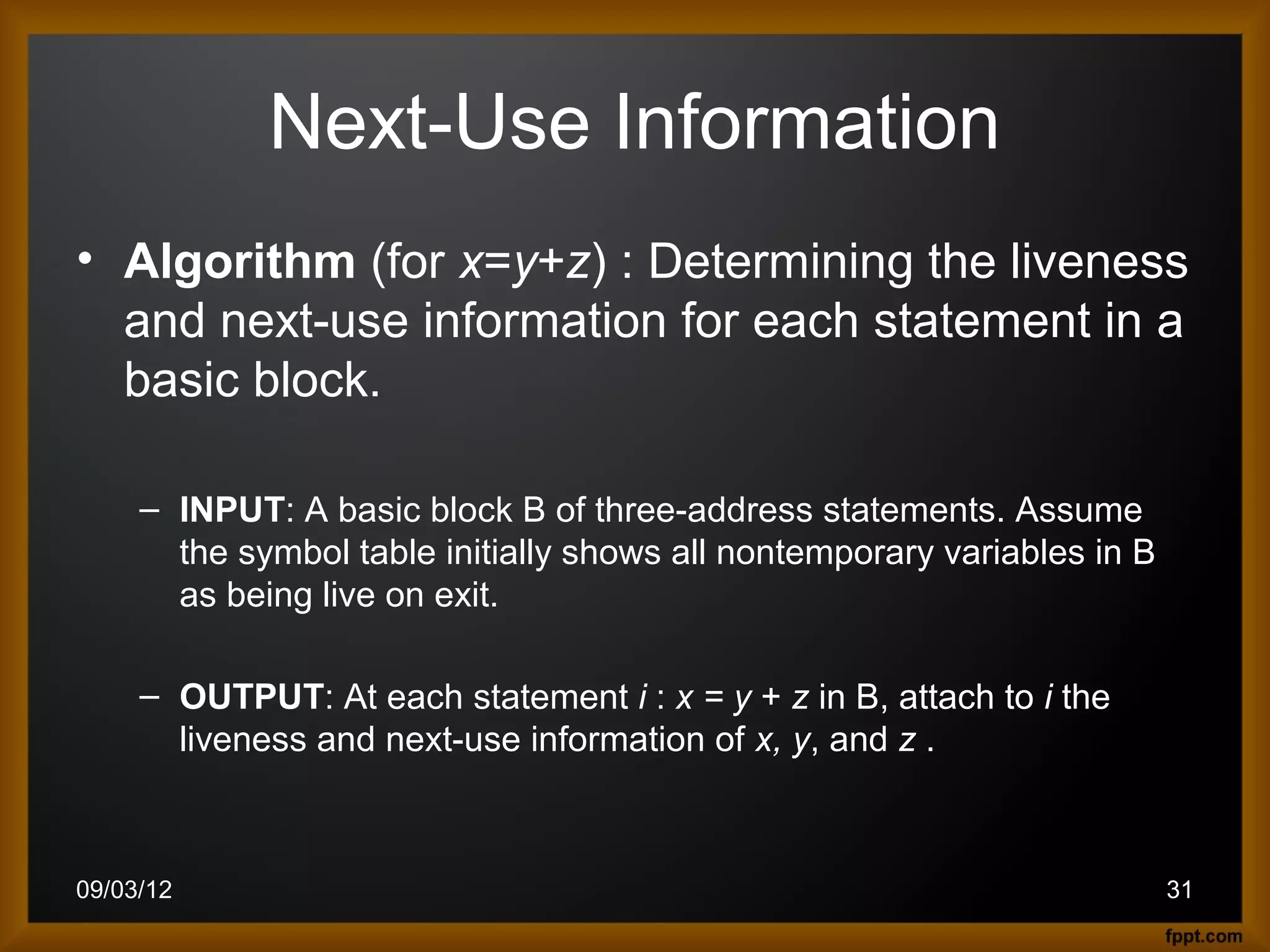
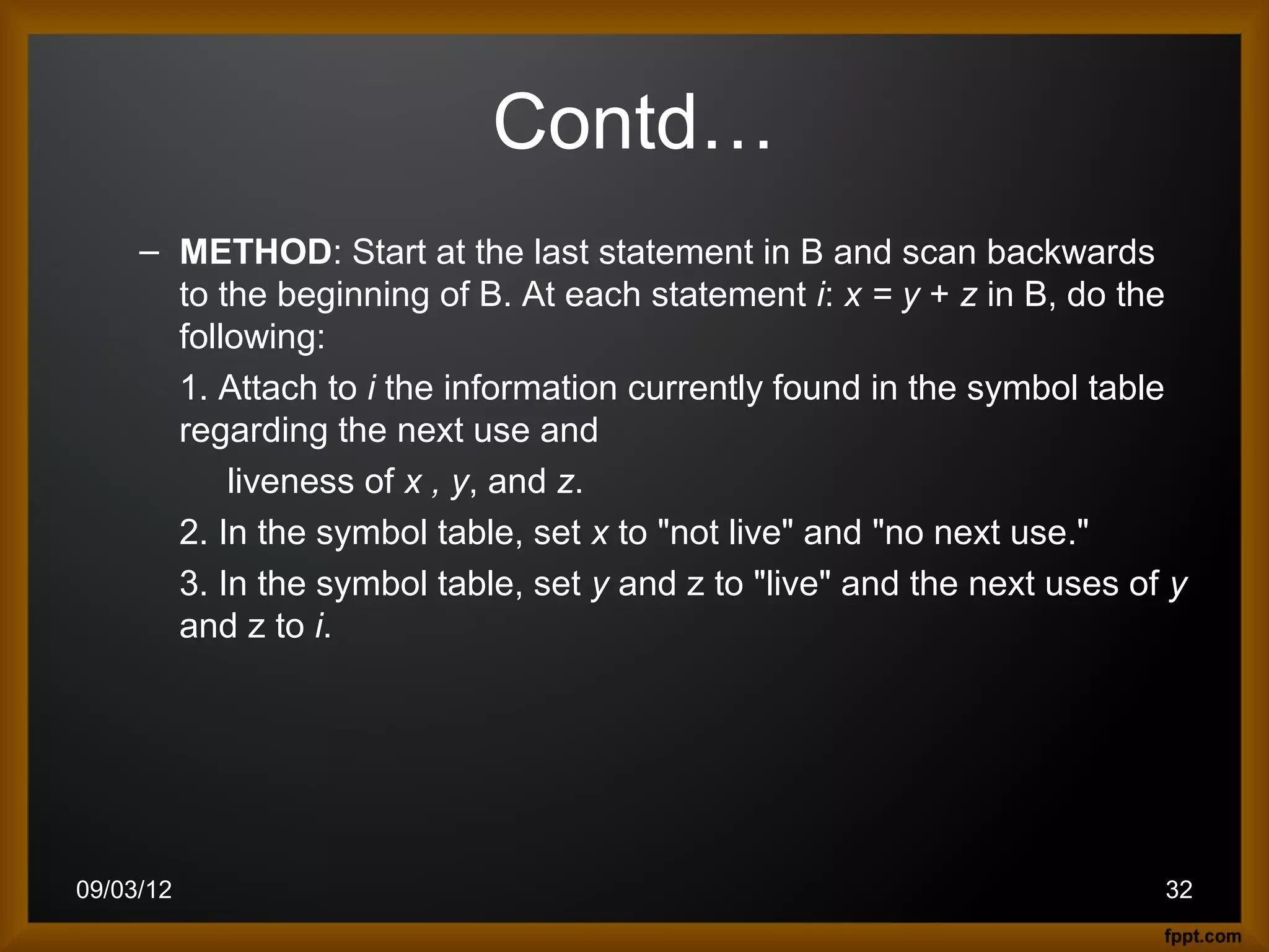
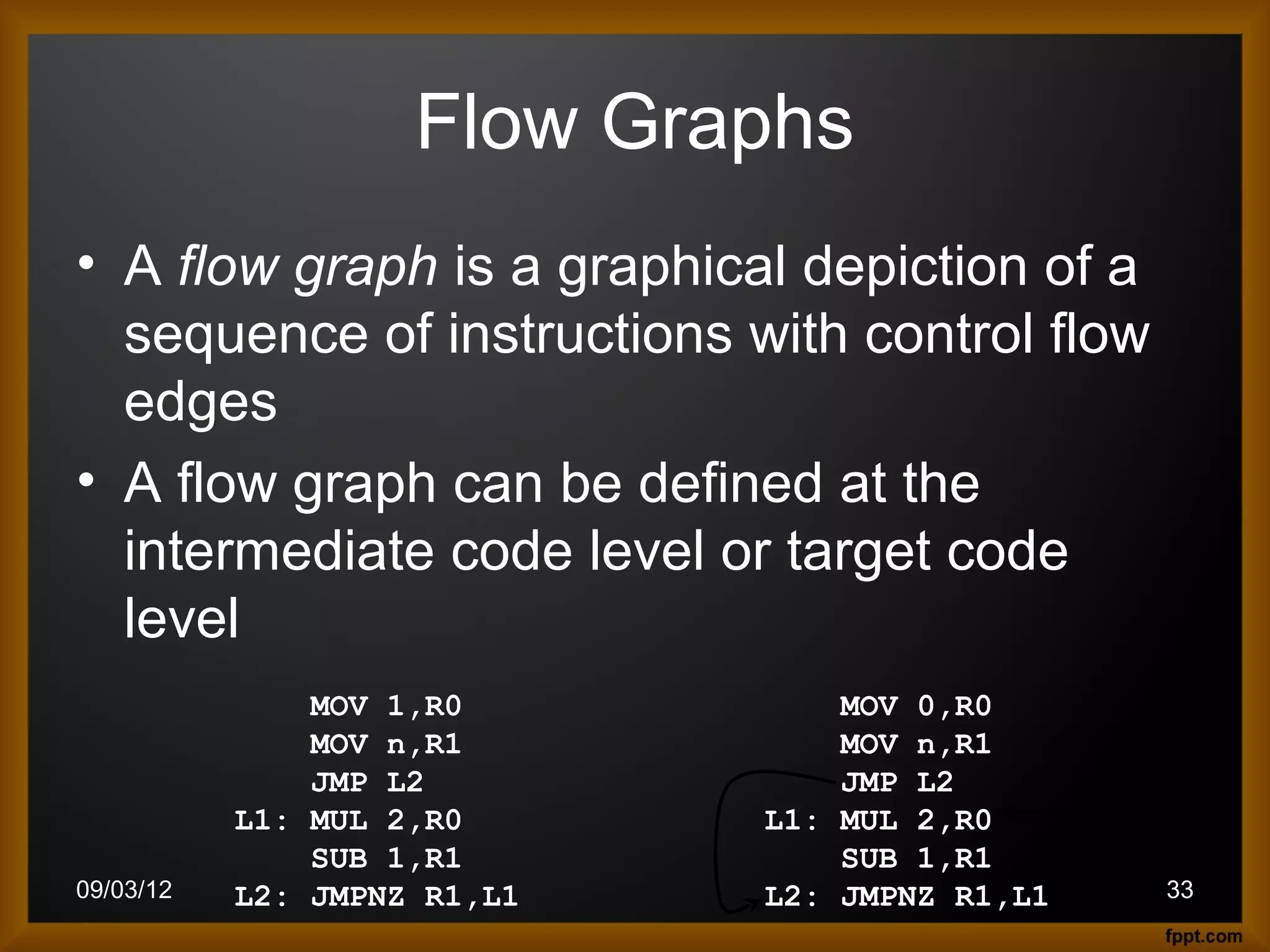
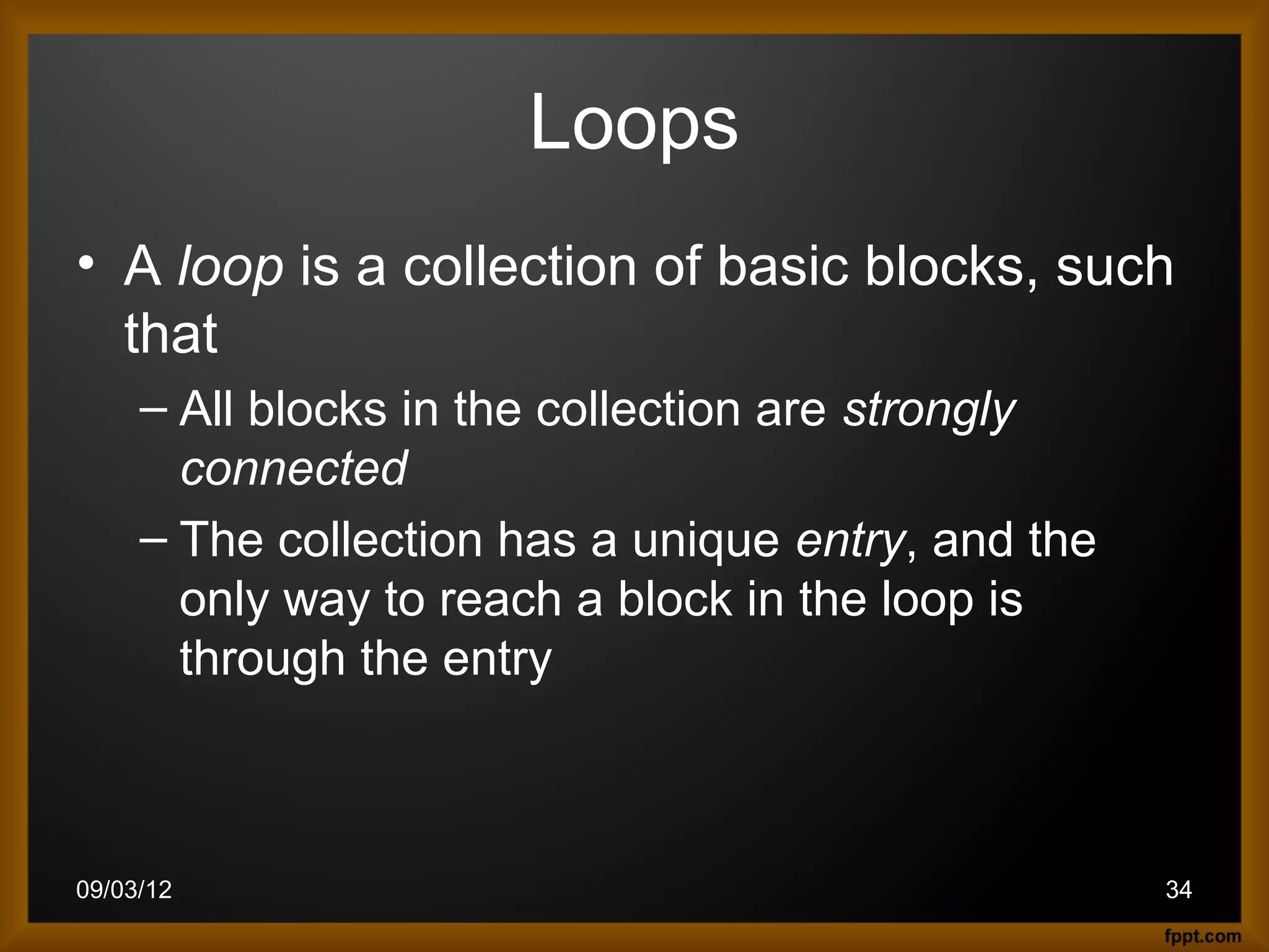
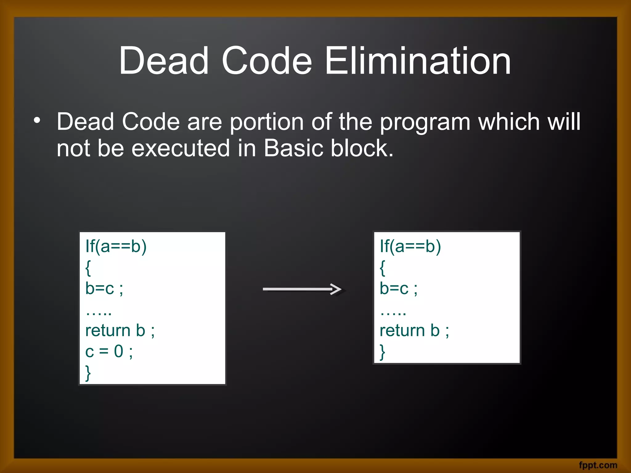
The document discusses code generation which is the final phase of a compiler that generates target code such as assembly code by selecting memory locations for variables, translating instructions into assembly instructions, and assigning variables and results to registers, and it outlines some of the key issues in code generation such as handling the input representation, the target language, instruction selection, register allocation, and evaluation order.

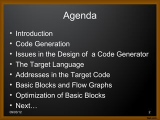

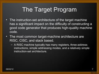
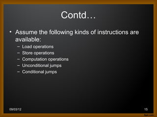
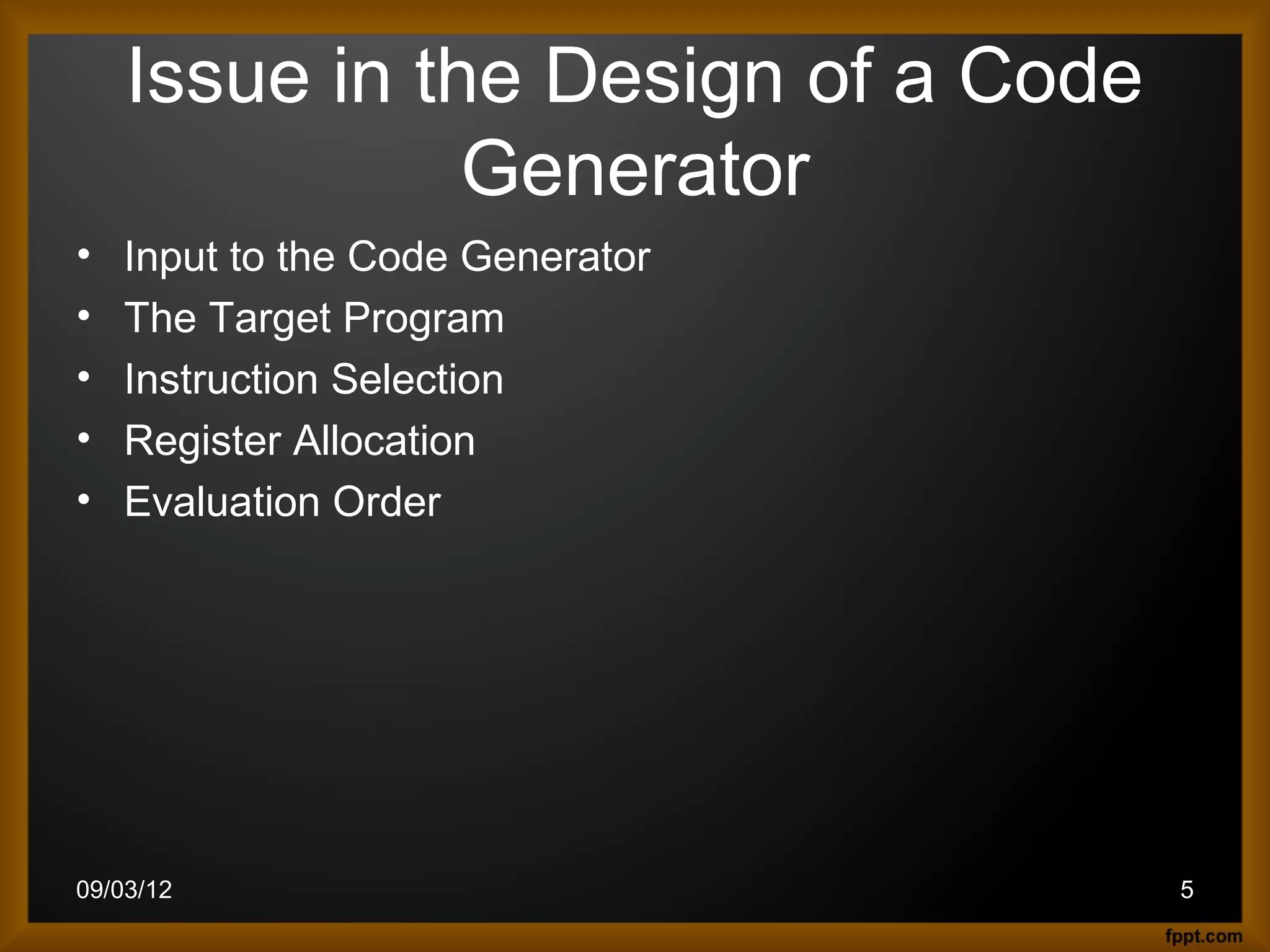
![A Simple Target Machine Model
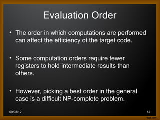
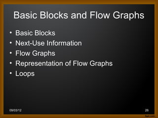
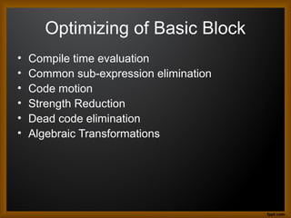
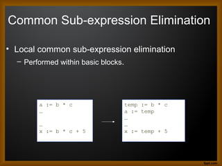
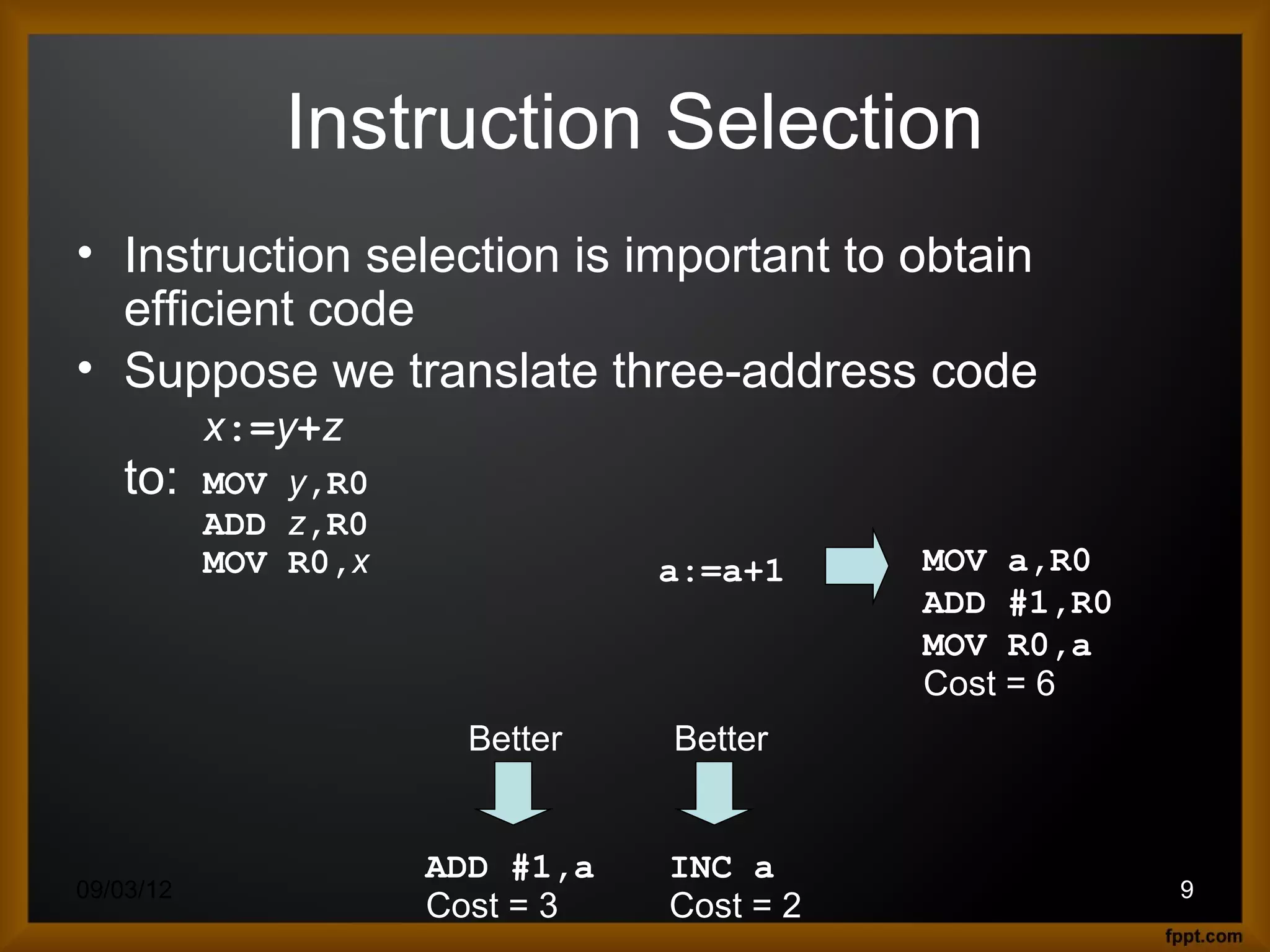
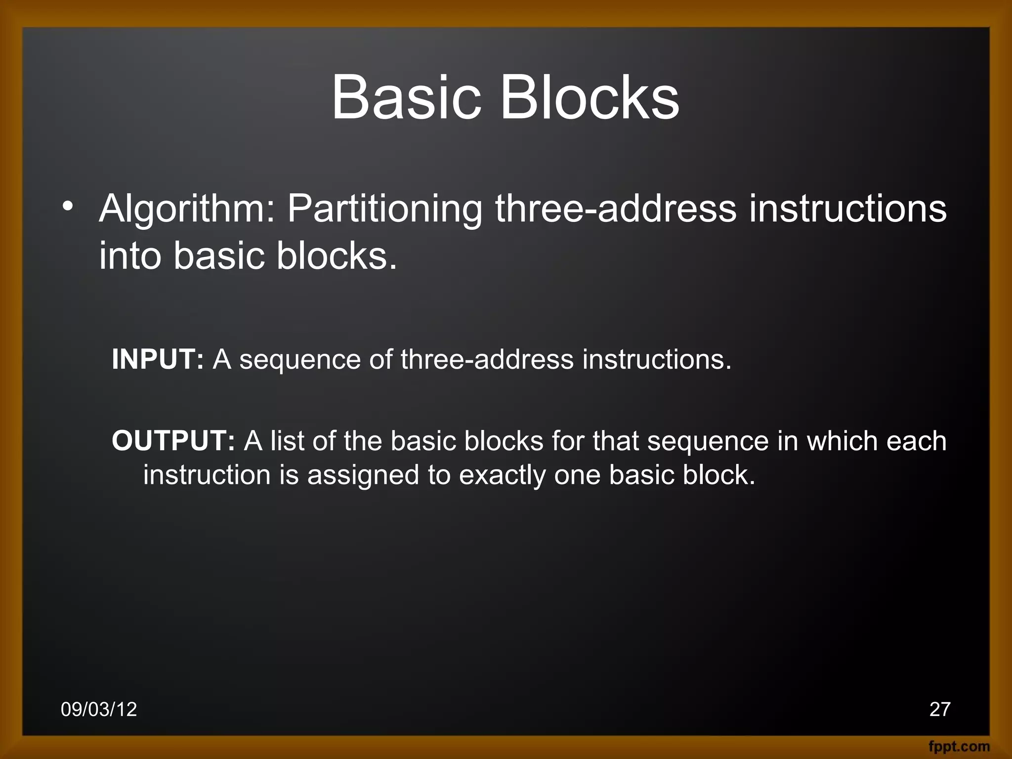
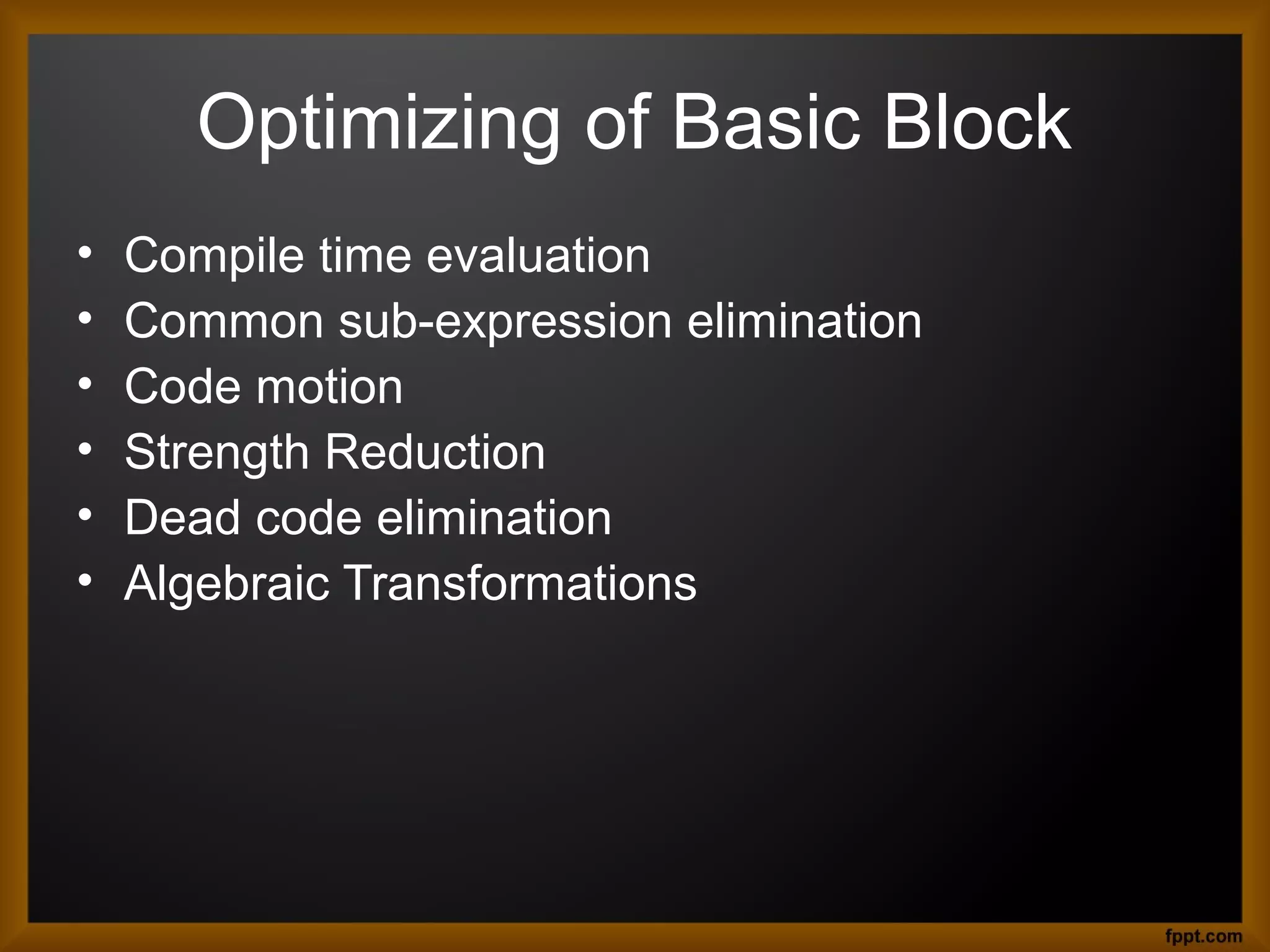
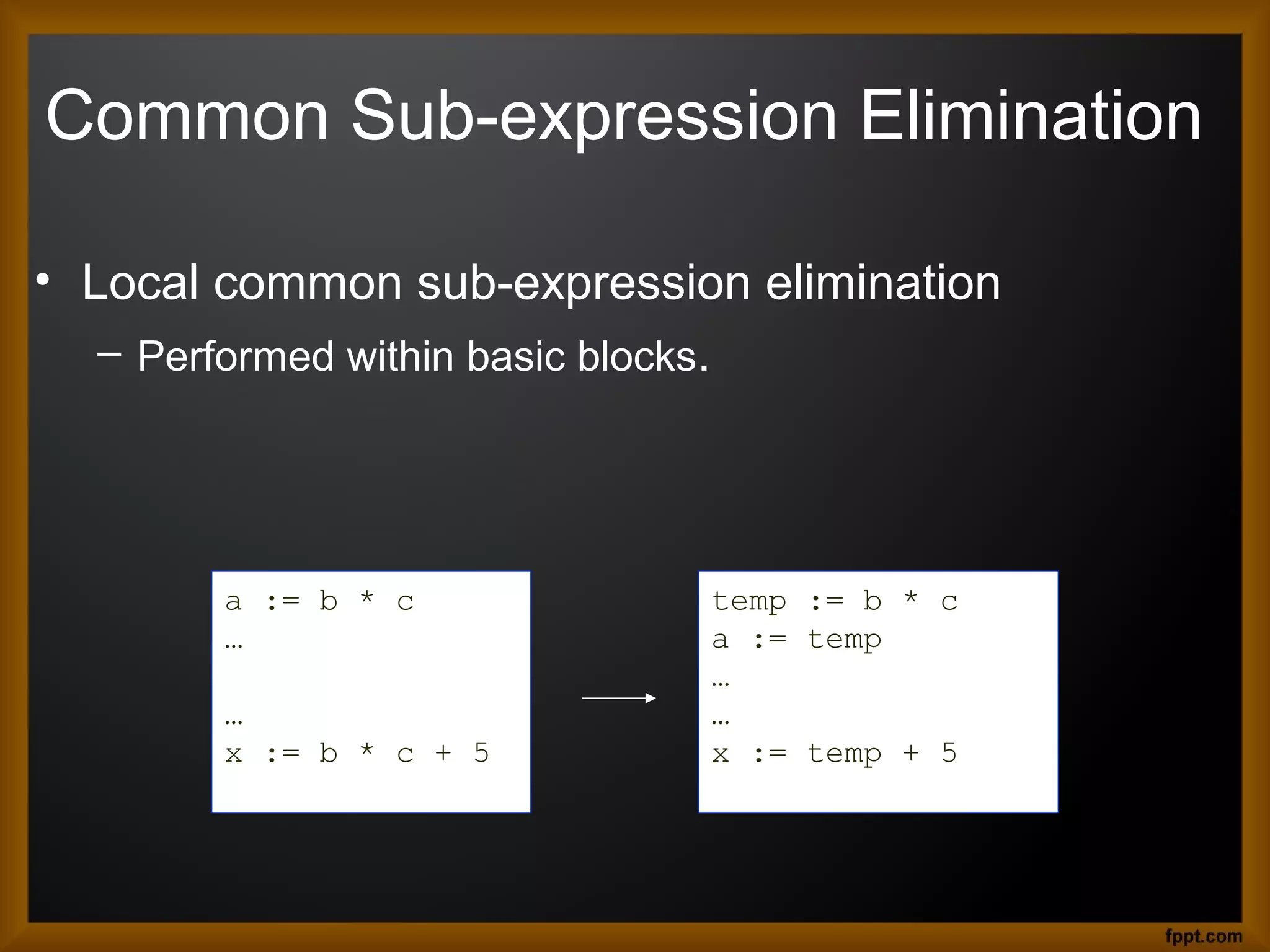
• Example :
x = y –z ⇒ LD R1, y x = *p ⇒ LD R1, p
LD R2, z LD R2, 0(R1)
SUB R1, R1, R2 ST x, R2
ST x, R1
b = a[i] ⇒ LD R1, i *p = y ⇒ LD R1, p
MUL R1, R1, 8 LD R2, y
LD R2, a(R1) ST 0(R1), R2
ST b, R2
09/03/12 17](https://image.slidesharecdn.com/codegenerator-120903115003-phpapp02/85/Code-generator-17-320.jpg)
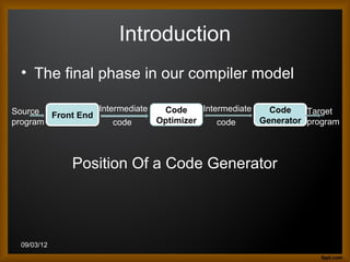
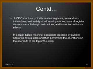
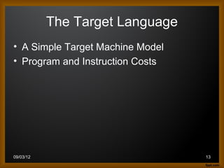
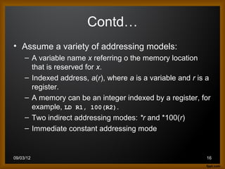
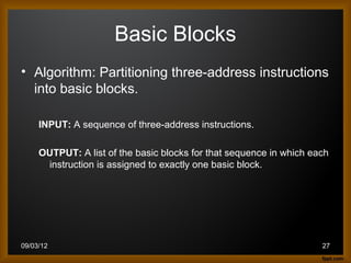
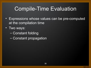
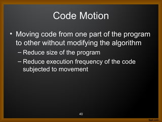
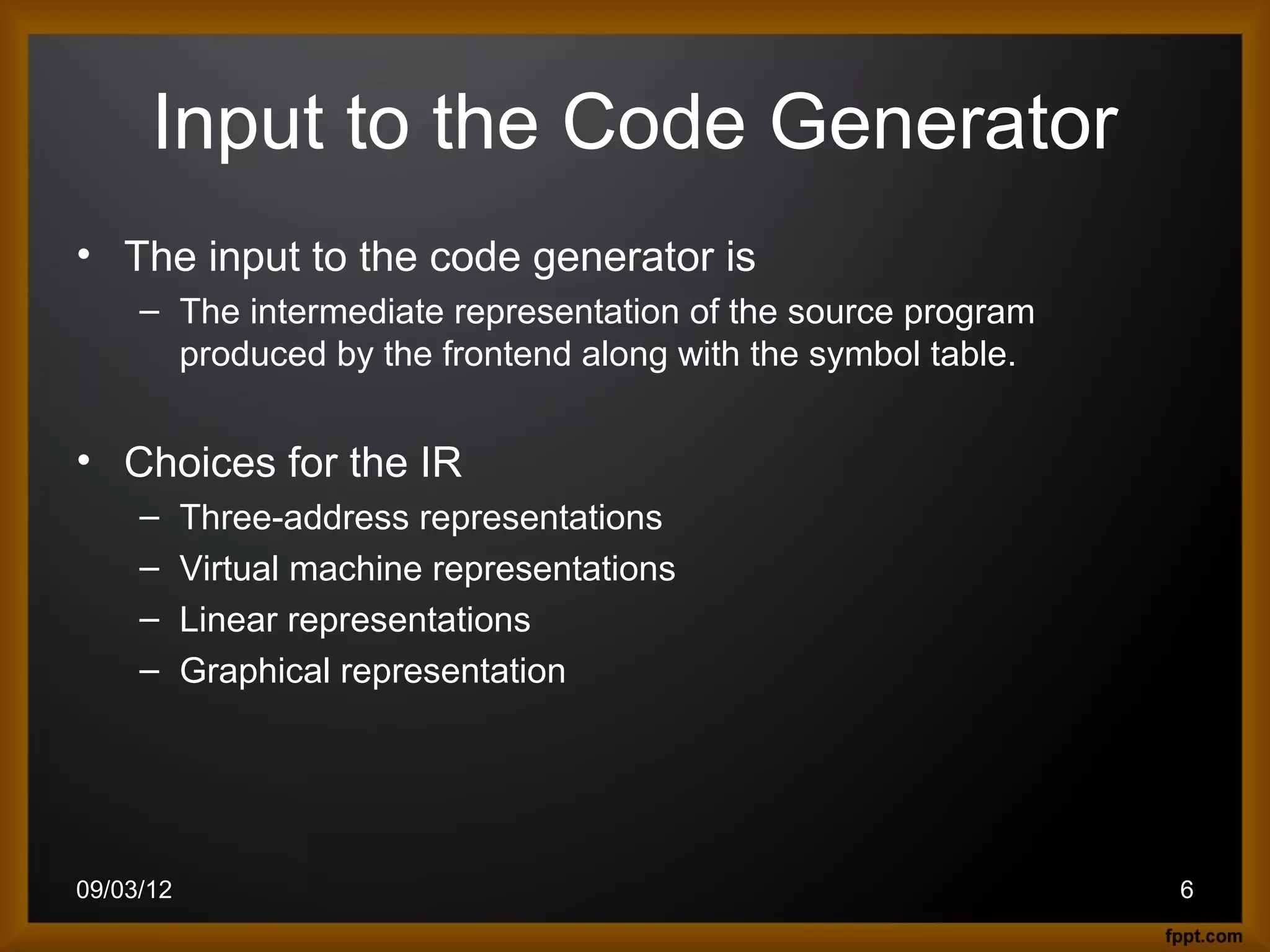
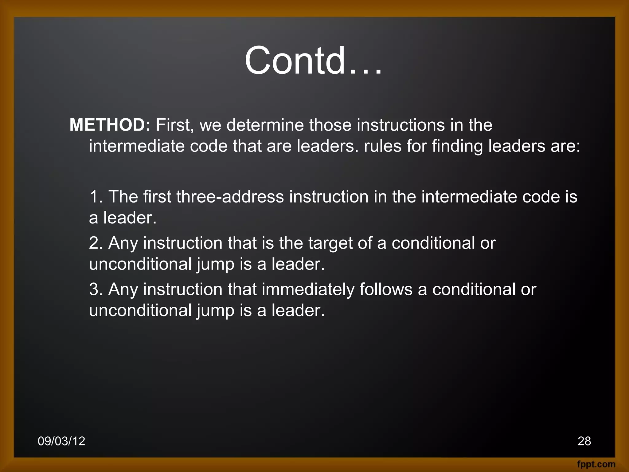
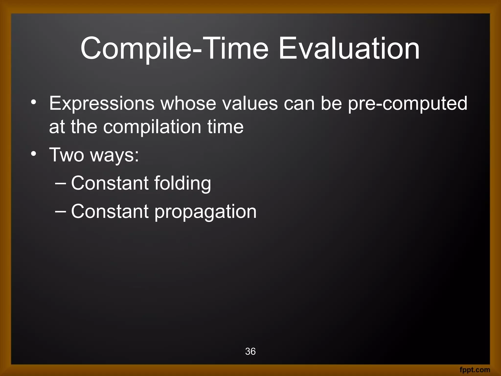
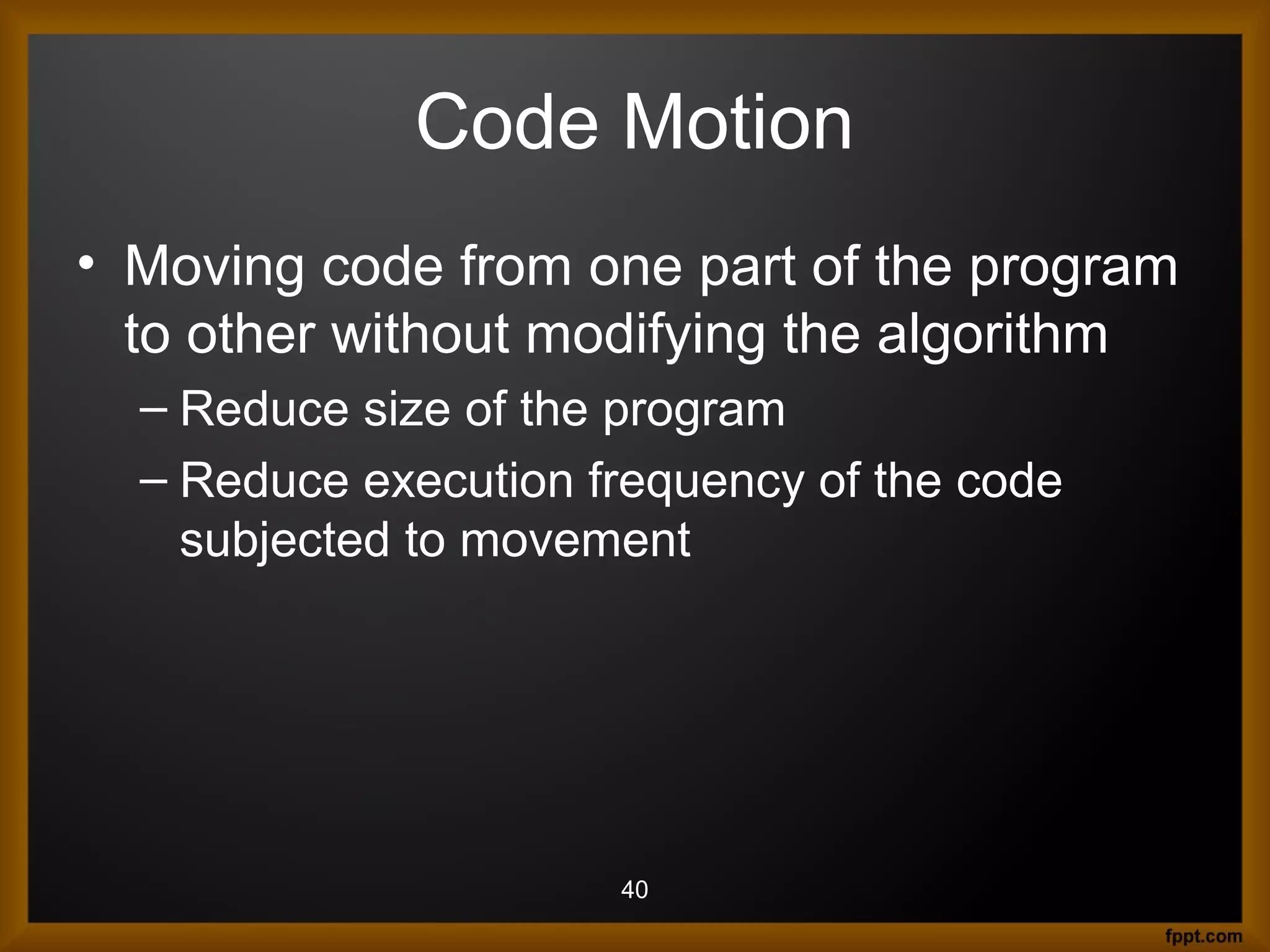
![a[j] = c ⇒ LD R1, c
LD R2, j
MUL R2, R2, 8
ST a(R2), R1
if x < y goto L ⇒ LD R1, x
LD R2, y
SUB R1, R1, R2
BLTZ R1, L
09/03/12 18](https://image.slidesharecdn.com/codegenerator-120903115003-phpapp02/85/Code-generator-18-320.jpg)
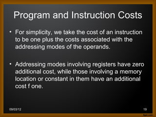
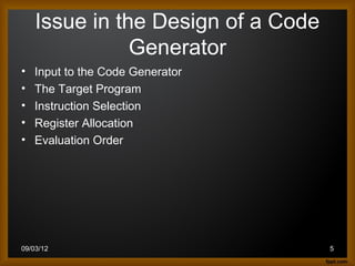
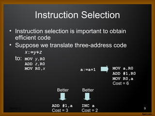
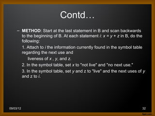
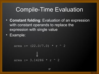
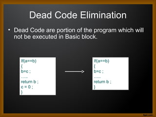
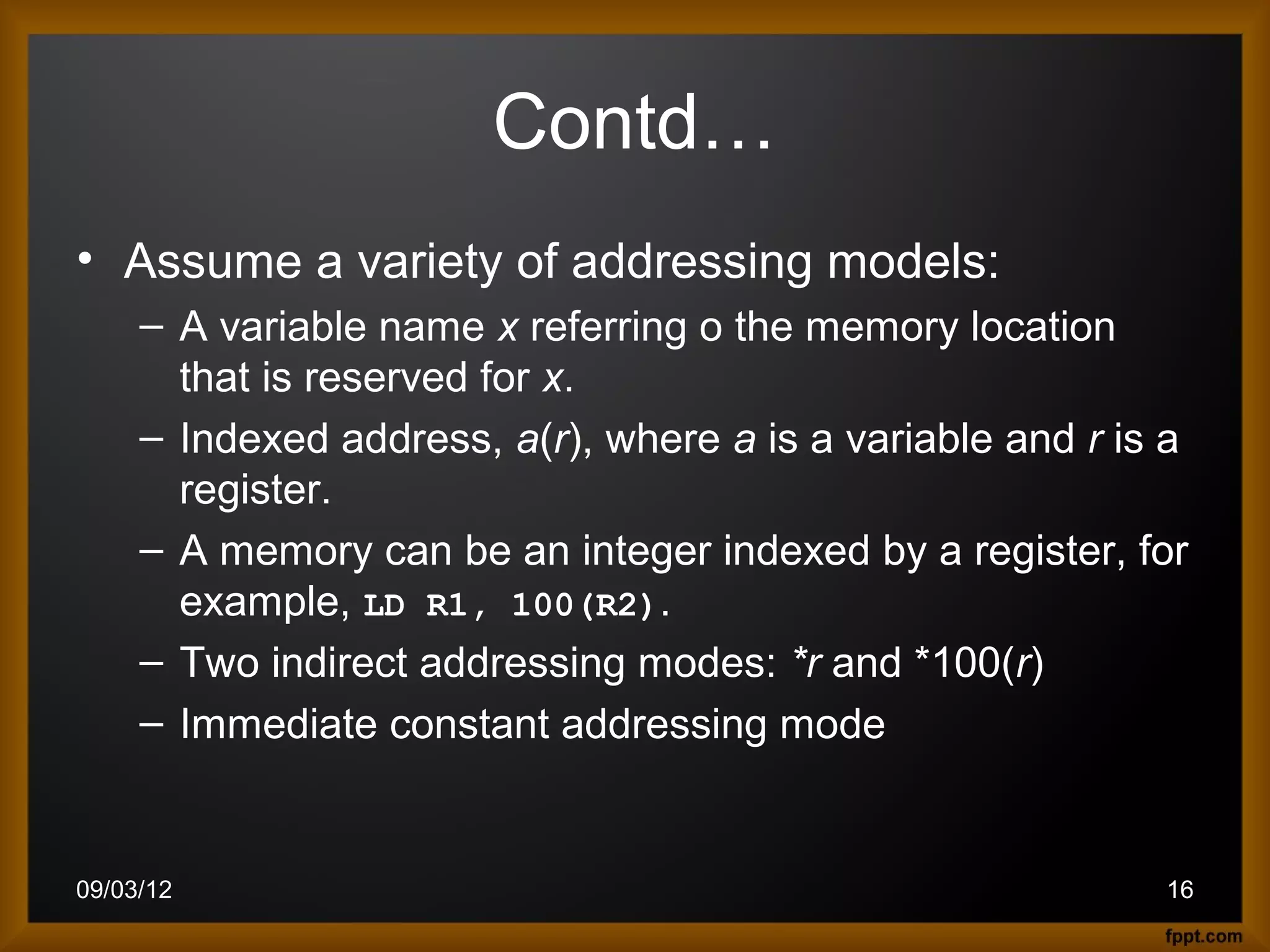
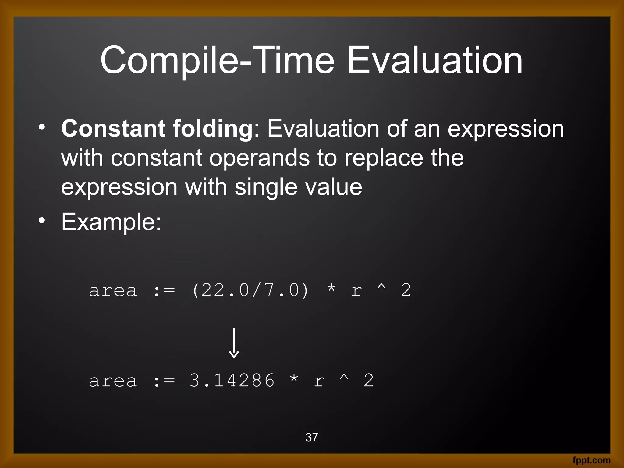
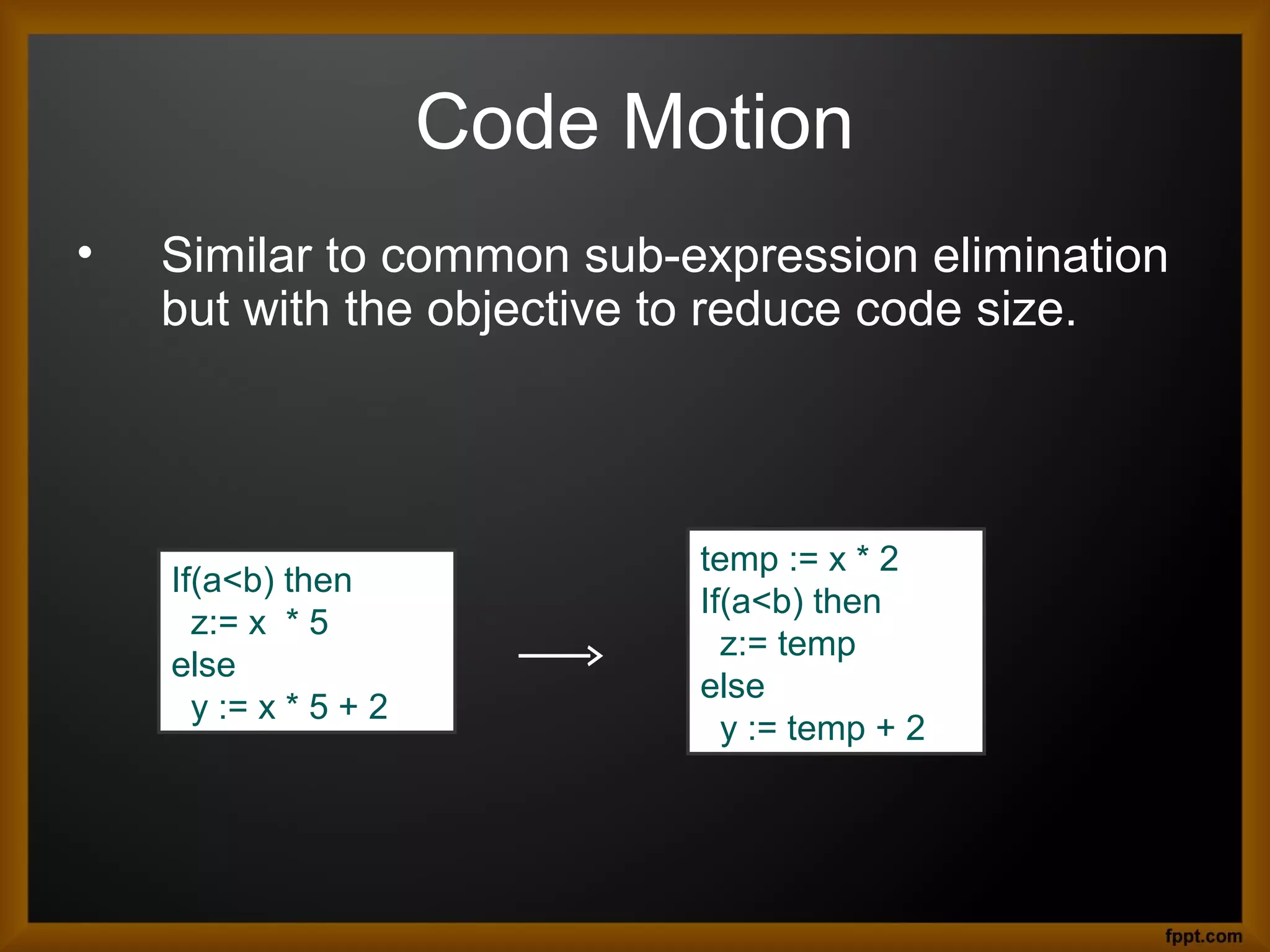
![Contd…
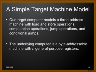
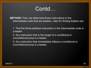
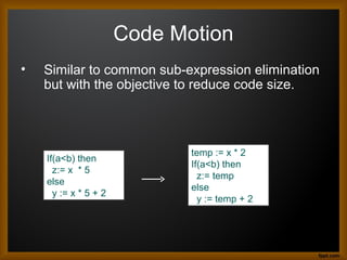
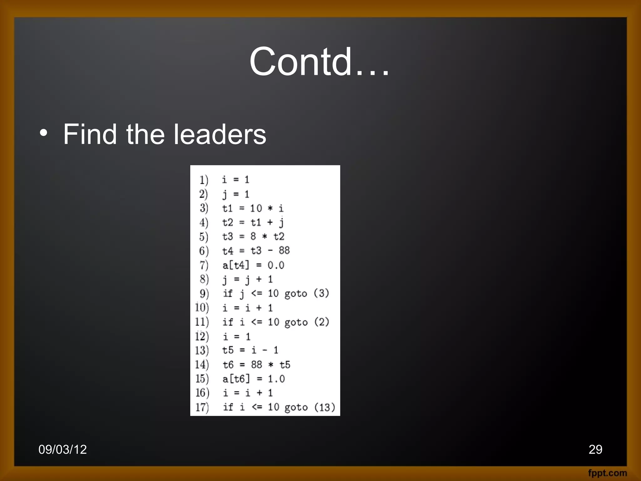
• Example:
– x=0
– Suppose the symbol-table entry for x contains a relative address
12
– x is in a statically allocated area beginning at address static
– the actual run-time address of x is static + 12
– The actual assignment: static [ 12] = 0
– For a static area starting at address 100: LD 112, #0
09/03/12 25](https://image.slidesharecdn.com/codegenerator-120903115003-phpapp02/85/Code-generator-25-320.jpg)

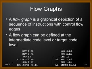

![A Simple Target Machine Model
• Example :
x = y –z ⇒ LD R1, y x = *p ⇒ LD R1, p
LD R2, z LD R2, 0(R1)
SUB R1, R1, R2 ST x, R2
ST x, R1
b = a[i] ⇒ LD R1, i *p = y ⇒ LD R1, p
MUL R1, R1, 8 LD R2, y
LD R2, a(R1) ST 0(R1), R2
ST b, R2
09/03/12 17](https://image.slidesharecdn.com/codegenerator-120903115003-phpapp02/75/Code-generator-17-2048.jpg)
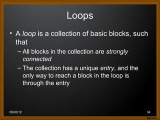
![a[j] = c ⇒ LD R1, c
LD R2, j
MUL R2, R2, 8
ST a(R2), R1
if x < y goto L ⇒ LD R1, x
LD R2, y
SUB R1, R1, R2
BLTZ R1, L
09/03/12 18](https://image.slidesharecdn.com/codegenerator-120903115003-phpapp02/75/Code-generator-18-2048.jpg)
![Contd…
• Example:
– x=0
– Suppose the symbol-table entry for x contains a relative address
12
– x is in a statically allocated area beginning at address static
– the actual run-time address of x is static + 12
– The actual assignment: static [ 12] = 0
– For a static area starting at address 100: LD 112, #0
09/03/12 25](https://image.slidesharecdn.com/codegenerator-120903115003-phpapp02/75/Code-generator-25-2048.jpg)


![UiPath Automation Suite Installation (Hands-On) [2/3]](https://cdn.slidesharecdn.com/ss_thumbnails/automationsuitecommunitysession2-251015095633-a6d862f1-thumbnail.jpg?width=600ounds&width=560&fit=bounds)