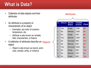
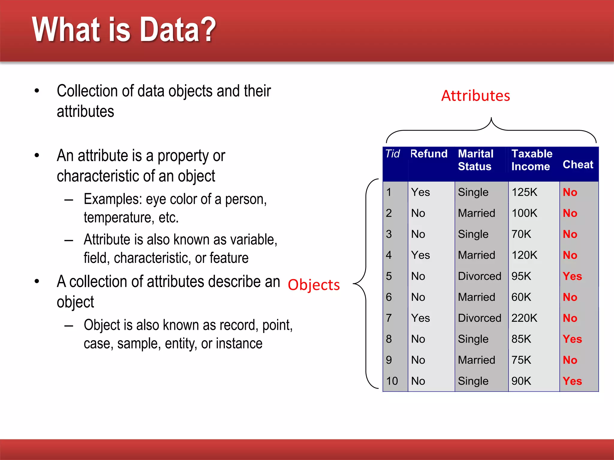
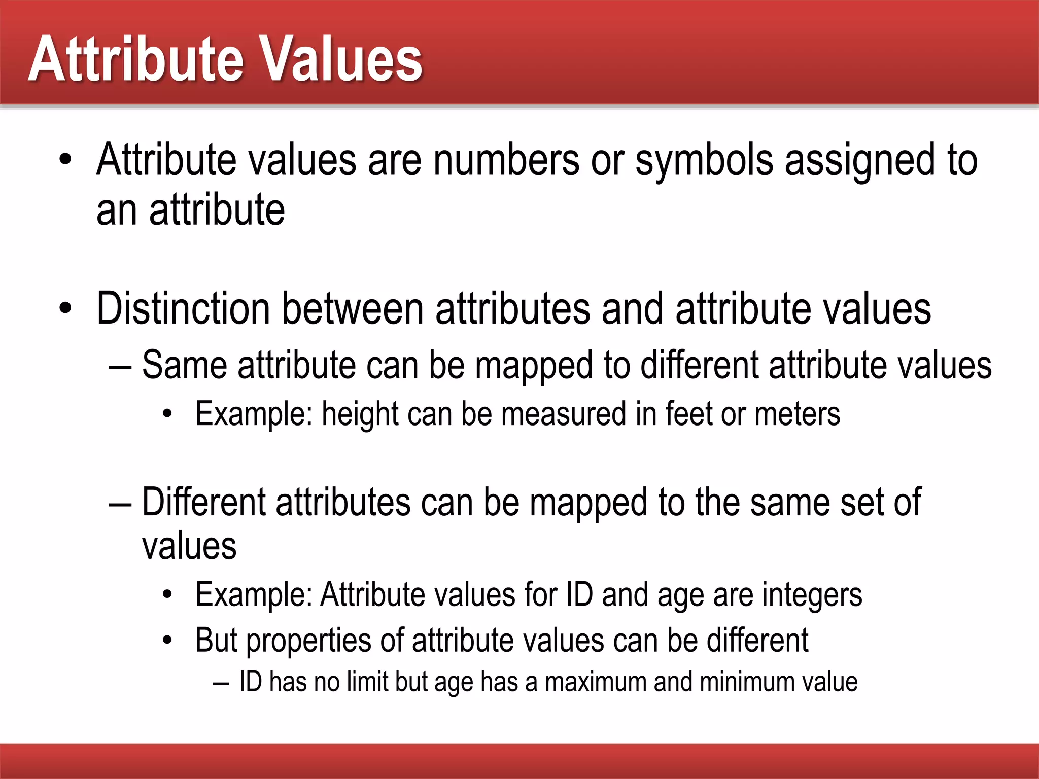
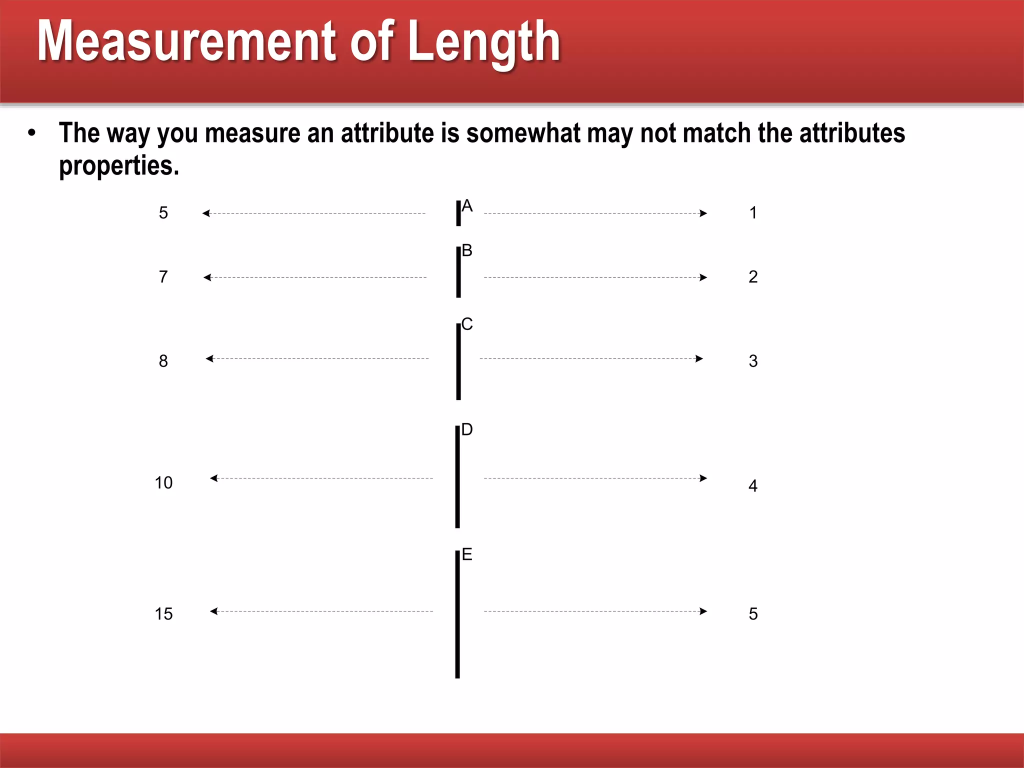
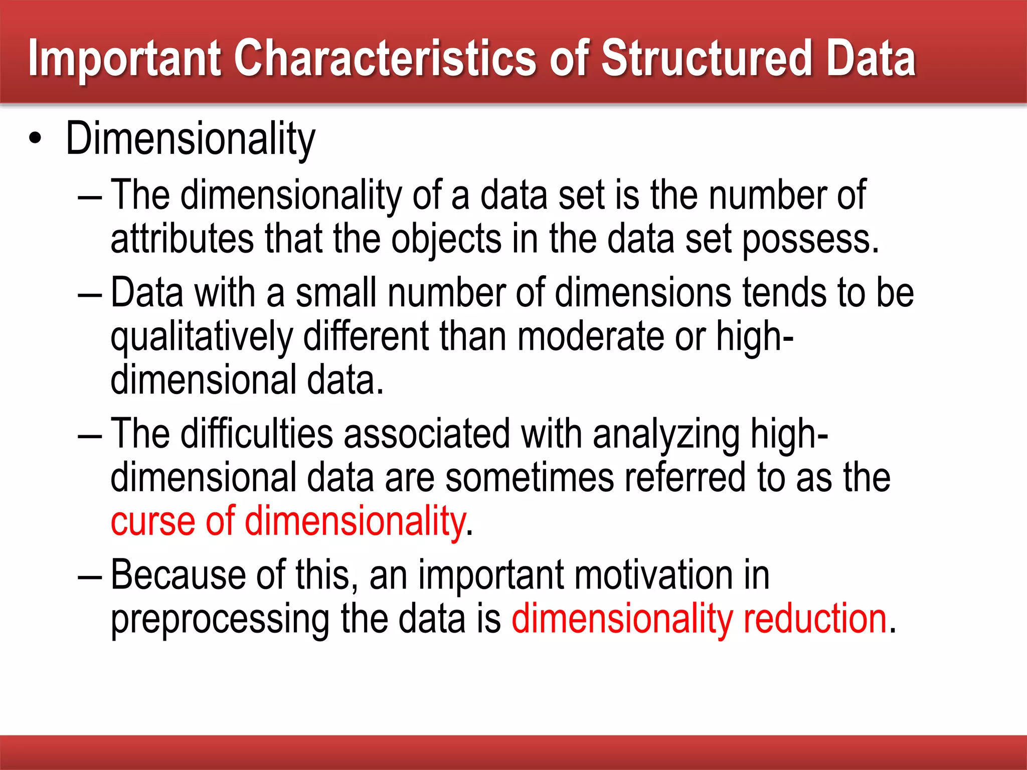
KEMBAR78
Data mining Basics and complete description | PPTX
Data Mining
Lecture – 02
What is Data?
• Collection of data objects and their
attributes
• An attribute is a property or
characteristic of an object
– Examples: eye color of a person,
temperature, etc.
– Attribute is also known as variable,
field, characteristic, or feature
• A collection of attributes describe an
object
– Object is also known as record, point,
case, sample, entity, or instance
Tid Refund Marital
Status
Taxable
Income Cheat
1 Yes Single 125K No
2 No Married 100K No
3 No Single 70K No
4 Yes Married 120K No
5 No Divorced 95K Yes
6 No Married 60K No
7 Yes Divorced 220K No
8 No Single 85K Yes
9 No Married 75K No
10 No Single 90K Yes
10
Attributes
Objects
Attribute Values
• Attribute values are numbers or symbols assigned to
an attribute
• Distinction between attributes and attribute values
– Same attribute can be mapped to different attribute values
• Example: height can be measured in feet or meters
– Different attributes can be mapped to the same set of
values
• Example: Attribute values for ID and age are integers
• But properties of attribute values can be different
– ID has no limit but age has a maximum and minimum value
Measurement of Length
• The way you measure an attribute is somewhat may not match the attributes
properties.
1
2
3
5
5
7
8
15
10 4
A
B
C
D
E
Types of Attributes
• There are different types of attributes
– Nominal
• Examples: ID numbers, eye color, zip codes
– Ordinal
• Examples: rankings (e.g., taste of potato chips on a scale from 1-
10), grades, height in {tall, medium, short}
– Interval
• Examples: calendar dates, temperatures in Celsius or Fahrenheit.
– Ratio
• Examples: temperature in Kelvin, length, time, counts
Properties of Attribute Values
• The type of an attribute depends on which of the
following properties it possesses:
– Distinctness: = 
– Order: < >
– Addition: + -
– Multiplication: * /
– Nominal attribute: distinctness
– Ordinal attribute: distinctness & order
– Interval attribute: distinctness, order & addition
– Ratio attribute: all 4 properties
Attribute Type Description Examples Operations
Nominal The values of a nominal attribute
are just different names, i.e.,
nominal attributes provide only
enough information to distinguish
one object from another. (=, )
zip codes, employee
ID numbers, eye
color, gender: {male,
female}
mode, entropy,
contingency
correlation, 2 test
Ordinal The values of an ordinal attribute
provide enough information to order
objects. (<, >)
hardness of minerals,
{good, better, best},
grades, street
numbers
median,
percentiles, rank
correlation, run
tests, sign tests
Interval For interval attributes, the
differences between values are
meaningful, i.e., a unit of
measurement exists.
(+, - )
calendar dates,
temperature in Celsius
or Fahrenheit
mean, standard
deviation,
Pearson's
correlation, t and F
tests
Ratio For ratio variables, both differences
and ratios are meaningful. (*, /)
temperature in Kelvin,
monetary quantities,
counts, age, mass,
length, electrical
current
geometric mean,
harmonic mean,
percent variation
Attribute
Level
Transformation Comments
Nominal Any permutation of values If all employee ID numbers
were reassigned, would it
make any difference?
Ordinal An order preserving change of values,
i.e.,
new_value = f(old_value)
where f is a monotonic function.
An attribute encompassing the
notion of good, better best can
be represented equally well by
the values {1, 2, 3} or by { 0.5,
1, 10}.
Interval new_value =a * old_value + b where a
and b are constants
Thus, the Fahrenheit and
Celsius temperature scales
differ in terms of where their
zero value is and the size of a
unit (degree).
Ratio new_value = a * old_value Length can be measured in
meters or feet.
Discrete and Continuous Attributes
• Discrete Attribute
– Has only a finite or countably infinite set of values
– Examples: zip codes, counts, or the set of words in a collection of documents
– Often represented as integer variables.
– Note: binary attributes are a special case of discrete attributes
• Continuous Attribute
– Has real numbers as attribute values
– Examples: temperature, height, or weight.
– Practically, real values can only be measured and represented using a finite number
of digits.
– Continuous attributes are typically represented as floating-point variables.
• Dimensionality
– The dimensionality of a data set is the number of
attributes that the objects in the data set possess.
– Data with a small number of dimensions tends to be
qualitatively different than moderate or high-
dimensional data.
– The difficulties associated with analyzing high-
dimensional data are sometimes referred to as the
curse of dimensionality.
– Because of this, an important motivation in
preprocessing the data is dimensionality reduction.
Important Characteristics of Structured Data
• Sparsity
– For some data sets, such as those with asymmetric
features, most attributes of an object have values of 0; in
many cases, fewer than 1% of the entries are non-zero.
– In a database, sparsity and density describe the number
of cells in a table that are empty (sparsity) and that
contain information (density), though sparse cells are not
always technically empty—they often contain a “0” digit.
– Sparsity is an advantage because usually only the non-
zero values need to be stored and manipulated.
Important Characteristics of Structured Data
• Resolution
– It is frequently possible to obtain data at different levels of resolution;
and often the properties of the data are different at different resolution.
– For instance, the surface of the Earth seems very uneven at a
resolution of a few meters, but is relatively smooth at a resolution of
tens of kilometers.
– The patterns in the data also depend on the level of resolution,
• if the resolution is too fine, a pattern may not be visible or may be buried in noise;
• if the resolution is too coarse, the pattern may disappear.
– For example, variations in atmospheric pressure on a scale of hours
reflect the movement of storms and other weather systems, whereas,
on a scale of months, such phenomena are not detectable.
Important Characteristics of Structured Data
• Record
– Data Matrix
– Document Data
– Transaction Data
• Graph
– World Wide Web
– Molecular Structures
• Ordered
– Spatial Data
– Temporal Data
– Sequential Data
– Genetic Sequence Data
Types of Data Sets
Record Data
• Data that consists of a collection of records, each of
which consists of a fixed set of attributes
Tid Refund Marital
Status
Taxable
Income Cheat
1 Yes Single 125K No
2 No Married 100K No
3 No Single 70K No
4 Yes Married 120K No
5 No Divorced 95K Yes
6 No Married 60K No
7 Yes Divorced 220K No
8 No Single 85K Yes
9 No Married 75K No
10 No Single 90K Yes
10
Data Matrix
• If data objects have the same fixed set of numeric attributes, then the data
objects can be thought of as points in a multi-dimensional space, where each
dimension represents a distinct attribute
• Such data set can be represented by an m by n matrix, where there are m
rows, one for each object, and n columns, one for each attribute
• A variation of record data, but because it consists of numeric attributes,
standard matrix operation can be applied to transform and manipulate the
data.
• Therefore, it is the standard format for most statistical data.
1.12.216.226.2512.65
1.22.715.225.2710.23
ThicknessLoadDistanceProjection
of y load
Projection
of x Load
1.12.216.226.2512.65
1.22.715.225.2710.23
ThicknessLoadDistanceProjection
of y load
Projection
of x Load
Document Data
• Each document becomes a `term' vector,
– each term is a component (attribute) of the vector,
– the value of each component is the number of times the
corresponding term occurs in the document.
Document 1
season
timeout
lost
wi
n
game
score
ball
pla
y
coach
team
Document 2
Document 3
3 0 5 0 2 6 0 2 0 2
0
0
7 0 2 1 0 0 3 0 0
1 0 0 1 2 2 0 3 0
Transaction Data
• A special type of record data, where
– each record (transaction) involves a set of items.
– For example, consider a grocery store. The set of products
purchased by a customer during one shopping trip constitute
a transaction, while the individual products that were
purchased are the items.
TID Items
1 Bread, Coke, Milk
2 Beer, Bread
3 Beer, Coke, Diaper, Milk
4 Beer, Bread, Diaper, Milk
5 Coke, Diaper, Milk
Graph Data
• Examples: Generic graph and HTML Links
5
2
1
2
5
<a href="papers/papers.html#bbbb">
Data Mining </a>
<li>
<a href="papers/papers.html#aaaa">
Graph Partitioning </a>
<li>
<a href="papers/papers.html#aaaa">
Parallel Solution of Sparse Linear System of Equations </a>
<li>
<a href="papers/papers.html#ffff">
N-Body Computation and Dense Linear System Solvers
Chemical Data
• Benzene Molecule: C6H6
Ordered Data
• Sequences of transactions
An element of the
sequence
Items/Events
Ordered Data
• Genomic sequence data
GGTTCCGCCTTCAGCCCCGCGCC
CGCAGGGCCCGCCCCGCGCCGTC
GAGAAGGGCCCGCCTGGCGGGCG
GGGGGAGGCGGGGCCGCCCGAGC
CCAACCGAGTCCGACCAGGTGCC
CCCTCTGCTCGGCCTAGACCTGA
GCTCATTAGGCGGCAGCGGACAG
GCCAAGTAGAACACGCGAAGCGC
TGGGCTGCCTGCTGCGACCAGGG
• Spatio-Temporal Data
Average Monthly
Temperature of land
and ocean
Ordered Data
Data Quality
• What kinds of data quality problems?
• How can we detect problems with the data?
• What can we do about these problems?
• Examples of data quality problems:
– Noise and outliers
– missing values
– duplicate data
Noise
• Noise refers to modification of original values
– Examples: distortion of a person’s voice when talking on a poor phone and “snow” on television
screen
• Techniques from signal/image processing are used to reduce noise.
Two Sine Waves Two Sine Waves + Noise
Outliers
• Outliers are data objects with characteristics that are
considerably different than most of the other data
objects in the data set; or
• Values of an attribute that are unusual with respect to
the typical values for that attribute
Missing Values
• Reasons for missing values
– Information is not collected
(e.g., people decline to give their age and weight)
– Attributes may not be applicable to all cases
(e.g., annual income is not applicable to children)
• Handling missing values
– Eliminate Data Objects
– Estimate Missing Values
– Ignore the Missing Value During Analysis
– Replace with all possible values (weighted by their
probabilities)
Duplicate Data
• Data set may include data objects that are duplicates, or
almost duplicates of one another
– Major issue when merging data from heterogeous sources
• Examples:
– Same person with multiple email addresses
• Data cleaning
– Process of dealing with duplicate data issues
Data Preprocessing
• Aggregation
• Sampling
• Dimensionality Reduction
• Feature subset selection
• Feature creation
• Discretization and Binarization
• Attribute Transformation
Aggregation
• Combining two or more attributes (or objects) into a
single attribute (or object)
• Purpose
– Data reduction
• Reduce the number of attributes or objects
– Change of scale
• Cities aggregated into regions, states, countries, etc
– More “stable” data
• Aggregated data tends to have less variability
Aggregation
Standard Deviation of
Average Monthly
Precipitation
Standard Deviation of
Average Yearly Precipitation
Variation of Precipitation in Australia from 1982 to 1993
Sampling
• Sampling is the main technique employed for data
selection.
• It is often used for both the preliminary investigation of the
data and the final data analysis.
• Statisticians sample because obtaining the entire set of data
of interest is too expensive or time consuming.
• Sampling is used in data mining because processing the
entire set of data of interest is too expensive or time
consuming.
• In some cases, using a sampling algorithm can reduce the
data size to the point where a better, but more expensive
algorithm can be used.
Sampling …
• The key principle for effective sampling is the following:
– using a sample will work almost as well as using the entire
data sets, if the sample is representative
– A sample is representative if it has approximately the same
property (of interest) as the original set of data
• Sampling is a statistical process, the representativeness
of any particular sample will vary, and the best that we
can do is choose a sampling scheme that guarantees
a high probability of getting a representative sample.
Types of Sampling
• Simple Random Sampling
– There is an equal probability of selecting any particular item
1. Sampling without replacement
• As each item is selected, it is removed from the population
2. Sampling with replacement
• Objects are not removed from the population as they are selected for the sample.
– In sampling with replacement, the same object can be picked up more than once
• Stratified sampling
– Split the data into several partitions; then draw random
samples from each partition
8000 points 2000 Points 500 Points
Sample Size
• What sample size is necessary to get at least
one object from each of 10 groups.
Sample Size
• When dimensionality increases,
data becomes increasingly
sparse in the space that it
occupies
• Definitions of density and
distance between points, which
is critical for clustering and
outlier detection, become less
meaningful
• Randomly generate 500 points
• Compute difference between max and min
distance between any pair of points
Curse of Dimensionality
Dimensionality Reduction
• Techniques to reduce the dimensionality of a data set by
creating new attributes that are a combination of the old
attributes
• Purpose:
– Avoid curse of dimensionality
– Reduce amount of time and memory required by data mining
algorithms
– Lead to a more understandable model
– Allow data to be more easily visualized
– May help to eliminate irrelevant features or reduce noise
• Techniques
– Principle Component Analysis
– Singular Value Decomposition
– Others: supervised and non-linear techniques
Dimensionality Reduction: PCA
• Most common approach for dimensionality reduction
• PCA is a linear algebra technique for continuous
attributes that find new attributes (principal components)
that are linear combination of the original attributes
• Goal is to find a projection that captures the largest
amount of variation in data
Feature Subset Selection
• Another way to reduce dimensionality of data to use only a
subset of the features
• Redundant features
– duplicate much or all of the information contained in one or more
other attributes
– Example: purchase price of a product and the amount of sales tax
paid
• Irrelevant features
– contain no information that is useful for the data mining task at
hand
– Example: students' ID is often irrelevant to the task of predicting
students' GPA
Feature Subset Selection
• Techniques:
– Brute-force approch:
• Try all possible feature subsets as input to data mining algorithm
– Embedded approaches:
• Feature selection occurs naturally as part of the data mining
algorithm
– Filter approaches:
• Features are selected before data mining algorithm is run
– Wrapper approaches:
• Use the data mining algorithm as a black box to find best subset
of attributes
Feature Subset Selection - Process
41
Feature Creation
• Create new attributes that can capture the important
information in a data set much more efficiently than the
original attributes
• Three general methodologies:
– Feature Extraction
• domain-specific
– Mapping Data to New Space
– Feature Construction
• combining features
Feature Extraction
• The creation of a new set of features from the original
raw data is known as feature extraction.
– For example: a set of photographs, where each photograph
is to be classified according to whether or not it contains
human face. The raw data is a set of pixels and is not
suitable for many types of classification algorithms.
– However, if the data is processed to provide higher level
features, such as the presence or absence of certain types of
edges and areas that are highly correlated with the presence
of human faces, then a much broader set of classification
techniques can be applied to this problem.
43
Two Sine Waves Two Sine Waves + Noise Frequency
 Fourier transform
 Wavelet transform
Mapping Data to a New Space

Data mining Basics and complete description

  • 1.
  • 2.
    What is Data? •Collection of data objects and their attributes • An attribute is a property or characteristic of an object – Examples: eye color of a person, temperature, etc. – Attribute is also known as variable, field, characteristic, or feature • A collection of attributes describe an object – Object is also known as record, point, case, sample, entity, or instance Tid Refund Marital Status Taxable Income Cheat 1 Yes Single 125K No 2 No Married 100K No 3 No Single 70K No 4 Yes Married 120K No 5 No Divorced 95K Yes 6 No Married 60K No 7 Yes Divorced 220K No 8 No Single 85K Yes 9 No Married 75K No 10 No Single 90K Yes 10 Attributes Objects
  • 3.
    Attribute Values • Attributevalues are numbers or symbols assigned to an attribute • Distinction between attributes and attribute values – Same attribute can be mapped to different attribute values • Example: height can be measured in feet or meters – Different attributes can be mapped to the same set of values • Example: Attribute values for ID and age are integers • But properties of attribute values can be different – ID has no limit but age has a maximum and minimum value
  • 4.
    Measurement of Length •The way you measure an attribute is somewhat may not match the attributes properties. 1 2 3 5 5 7 8 15 10 4 A B C D E
  • 5.
    Types of Attributes •There are different types of attributes – Nominal • Examples: ID numbers, eye color, zip codes – Ordinal • Examples: rankings (e.g., taste of potato chips on a scale from 1- 10), grades, height in {tall, medium, short} – Interval • Examples: calendar dates, temperatures in Celsius or Fahrenheit. – Ratio • Examples: temperature in Kelvin, length, time, counts
  • 6.
    Properties of AttributeValues • The type of an attribute depends on which of the following properties it possesses: – Distinctness: =  – Order: < > – Addition: + - – Multiplication: * / – Nominal attribute: distinctness – Ordinal attribute: distinctness & order – Interval attribute: distinctness, order & addition – Ratio attribute: all 4 properties
  • 7.
    Attribute Type DescriptionExamples Operations Nominal The values of a nominal attribute are just different names, i.e., nominal attributes provide only enough information to distinguish one object from another. (=, ) zip codes, employee ID numbers, eye color, gender: {male, female} mode, entropy, contingency correlation, 2 test Ordinal The values of an ordinal attribute provide enough information to order objects. (<, >) hardness of minerals, {good, better, best}, grades, street numbers median, percentiles, rank correlation, run tests, sign tests Interval For interval attributes, the differences between values are meaningful, i.e., a unit of measurement exists. (+, - ) calendar dates, temperature in Celsius or Fahrenheit mean, standard deviation, Pearson's correlation, t and F tests Ratio For ratio variables, both differences and ratios are meaningful. (*, /) temperature in Kelvin, monetary quantities, counts, age, mass, length, electrical current geometric mean, harmonic mean, percent variation
  • 8.
    Attribute Level Transformation Comments Nominal Anypermutation of values If all employee ID numbers were reassigned, would it make any difference? Ordinal An order preserving change of values, i.e., new_value = f(old_value) where f is a monotonic function. An attribute encompassing the notion of good, better best can be represented equally well by the values {1, 2, 3} or by { 0.5, 1, 10}. Interval new_value =a * old_value + b where a and b are constants Thus, the Fahrenheit and Celsius temperature scales differ in terms of where their zero value is and the size of a unit (degree). Ratio new_value = a * old_value Length can be measured in meters or feet.
  • 9.
    Discrete and ContinuousAttributes • Discrete Attribute – Has only a finite or countably infinite set of values – Examples: zip codes, counts, or the set of words in a collection of documents – Often represented as integer variables. – Note: binary attributes are a special case of discrete attributes • Continuous Attribute – Has real numbers as attribute values – Examples: temperature, height, or weight. – Practically, real values can only be measured and represented using a finite number of digits. – Continuous attributes are typically represented as floating-point variables.
  • 10.
    • Dimensionality – Thedimensionality of a data set is the number of attributes that the objects in the data set possess. – Data with a small number of dimensions tends to be qualitatively different than moderate or high- dimensional data. – The difficulties associated with analyzing high- dimensional data are sometimes referred to as the curse of dimensionality. – Because of this, an important motivation in preprocessing the data is dimensionality reduction. Important Characteristics of Structured Data
  • 11.
    • Sparsity – Forsome data sets, such as those with asymmetric features, most attributes of an object have values of 0; in many cases, fewer than 1% of the entries are non-zero. – In a database, sparsity and density describe the number of cells in a table that are empty (sparsity) and that contain information (density), though sparse cells are not always technically empty—they often contain a “0” digit. – Sparsity is an advantage because usually only the non- zero values need to be stored and manipulated. Important Characteristics of Structured Data
  • 12.
    • Resolution – Itis frequently possible to obtain data at different levels of resolution; and often the properties of the data are different at different resolution. – For instance, the surface of the Earth seems very uneven at a resolution of a few meters, but is relatively smooth at a resolution of tens of kilometers. – The patterns in the data also depend on the level of resolution, • if the resolution is too fine, a pattern may not be visible or may be buried in noise; • if the resolution is too coarse, the pattern may disappear. – For example, variations in atmospheric pressure on a scale of hours reflect the movement of storms and other weather systems, whereas, on a scale of months, such phenomena are not detectable. Important Characteristics of Structured Data
  • 13.
    • Record – DataMatrix – Document Data – Transaction Data • Graph – World Wide Web – Molecular Structures • Ordered – Spatial Data – Temporal Data – Sequential Data – Genetic Sequence Data Types of Data Sets
  • 14.
    Record Data • Datathat consists of a collection of records, each of which consists of a fixed set of attributes Tid Refund Marital Status Taxable Income Cheat 1 Yes Single 125K No 2 No Married 100K No 3 No Single 70K No 4 Yes Married 120K No 5 No Divorced 95K Yes 6 No Married 60K No 7 Yes Divorced 220K No 8 No Single 85K Yes 9 No Married 75K No 10 No Single 90K Yes 10
  • 15.
    Data Matrix • Ifdata objects have the same fixed set of numeric attributes, then the data objects can be thought of as points in a multi-dimensional space, where each dimension represents a distinct attribute • Such data set can be represented by an m by n matrix, where there are m rows, one for each object, and n columns, one for each attribute • A variation of record data, but because it consists of numeric attributes, standard matrix operation can be applied to transform and manipulate the data. • Therefore, it is the standard format for most statistical data. 1.12.216.226.2512.65 1.22.715.225.2710.23 ThicknessLoadDistanceProjection of y load Projection of x Load 1.12.216.226.2512.65 1.22.715.225.2710.23 ThicknessLoadDistanceProjection of y load Projection of x Load
  • 16.
    Document Data • Eachdocument becomes a `term' vector, – each term is a component (attribute) of the vector, – the value of each component is the number of times the corresponding term occurs in the document. Document 1 season timeout lost wi n game score ball pla y coach team Document 2 Document 3 3 0 5 0 2 6 0 2 0 2 0 0 7 0 2 1 0 0 3 0 0 1 0 0 1 2 2 0 3 0
  • 17.
    Transaction Data • Aspecial type of record data, where – each record (transaction) involves a set of items. – For example, consider a grocery store. The set of products purchased by a customer during one shopping trip constitute a transaction, while the individual products that were purchased are the items. TID Items 1 Bread, Coke, Milk 2 Beer, Bread 3 Beer, Coke, Diaper, Milk 4 Beer, Bread, Diaper, Milk 5 Coke, Diaper, Milk
  • 18.
    Graph Data • Examples:Generic graph and HTML Links 5 2 1 2 5 <a href="papers/papers.html#bbbb"> Data Mining </a> <li> <a href="papers/papers.html#aaaa"> Graph Partitioning </a> <li> <a href="papers/papers.html#aaaa"> Parallel Solution of Sparse Linear System of Equations </a> <li> <a href="papers/papers.html#ffff"> N-Body Computation and Dense Linear System Solvers
  • 19.
  • 20.
    Ordered Data • Sequencesof transactions An element of the sequence Items/Events
  • 21.
    Ordered Data • Genomicsequence data GGTTCCGCCTTCAGCCCCGCGCC CGCAGGGCCCGCCCCGCGCCGTC GAGAAGGGCCCGCCTGGCGGGCG GGGGGAGGCGGGGCCGCCCGAGC CCAACCGAGTCCGACCAGGTGCC CCCTCTGCTCGGCCTAGACCTGA GCTCATTAGGCGGCAGCGGACAG GCCAAGTAGAACACGCGAAGCGC TGGGCTGCCTGCTGCGACCAGGG
  • 22.
    • Spatio-Temporal Data AverageMonthly Temperature of land and ocean Ordered Data
  • 23.
    Data Quality • Whatkinds of data quality problems? • How can we detect problems with the data? • What can we do about these problems? • Examples of data quality problems: – Noise and outliers – missing values – duplicate data
  • 24.
    Noise • Noise refersto modification of original values – Examples: distortion of a person’s voice when talking on a poor phone and “snow” on television screen • Techniques from signal/image processing are used to reduce noise. Two Sine Waves Two Sine Waves + Noise
  • 25.
    Outliers • Outliers aredata objects with characteristics that are considerably different than most of the other data objects in the data set; or • Values of an attribute that are unusual with respect to the typical values for that attribute
  • 26.
    Missing Values • Reasonsfor missing values – Information is not collected (e.g., people decline to give their age and weight) – Attributes may not be applicable to all cases (e.g., annual income is not applicable to children) • Handling missing values – Eliminate Data Objects – Estimate Missing Values – Ignore the Missing Value During Analysis – Replace with all possible values (weighted by their probabilities)
  • 27.
    Duplicate Data • Dataset may include data objects that are duplicates, or almost duplicates of one another – Major issue when merging data from heterogeous sources • Examples: – Same person with multiple email addresses • Data cleaning – Process of dealing with duplicate data issues
  • 28.
    Data Preprocessing • Aggregation •Sampling • Dimensionality Reduction • Feature subset selection • Feature creation • Discretization and Binarization • Attribute Transformation
  • 29.
    Aggregation • Combining twoor more attributes (or objects) into a single attribute (or object) • Purpose – Data reduction • Reduce the number of attributes or objects – Change of scale • Cities aggregated into regions, states, countries, etc – More “stable” data • Aggregated data tends to have less variability
  • 30.
    Aggregation Standard Deviation of AverageMonthly Precipitation Standard Deviation of Average Yearly Precipitation Variation of Precipitation in Australia from 1982 to 1993
  • 31.
    Sampling • Sampling isthe main technique employed for data selection. • It is often used for both the preliminary investigation of the data and the final data analysis. • Statisticians sample because obtaining the entire set of data of interest is too expensive or time consuming. • Sampling is used in data mining because processing the entire set of data of interest is too expensive or time consuming. • In some cases, using a sampling algorithm can reduce the data size to the point where a better, but more expensive algorithm can be used.
  • 32.
    Sampling … • Thekey principle for effective sampling is the following: – using a sample will work almost as well as using the entire data sets, if the sample is representative – A sample is representative if it has approximately the same property (of interest) as the original set of data • Sampling is a statistical process, the representativeness of any particular sample will vary, and the best that we can do is choose a sampling scheme that guarantees a high probability of getting a representative sample.
  • 33.
    Types of Sampling •Simple Random Sampling – There is an equal probability of selecting any particular item 1. Sampling without replacement • As each item is selected, it is removed from the population 2. Sampling with replacement • Objects are not removed from the population as they are selected for the sample. – In sampling with replacement, the same object can be picked up more than once • Stratified sampling – Split the data into several partitions; then draw random samples from each partition
  • 34.
    8000 points 2000Points 500 Points Sample Size
  • 35.
    • What samplesize is necessary to get at least one object from each of 10 groups. Sample Size
  • 36.
    • When dimensionalityincreases, data becomes increasingly sparse in the space that it occupies • Definitions of density and distance between points, which is critical for clustering and outlier detection, become less meaningful • Randomly generate 500 points • Compute difference between max and min distance between any pair of points Curse of Dimensionality
  • 37.
    Dimensionality Reduction • Techniquesto reduce the dimensionality of a data set by creating new attributes that are a combination of the old attributes • Purpose: – Avoid curse of dimensionality – Reduce amount of time and memory required by data mining algorithms – Lead to a more understandable model – Allow data to be more easily visualized – May help to eliminate irrelevant features or reduce noise • Techniques – Principle Component Analysis – Singular Value Decomposition – Others: supervised and non-linear techniques
  • 38.
    Dimensionality Reduction: PCA •Most common approach for dimensionality reduction • PCA is a linear algebra technique for continuous attributes that find new attributes (principal components) that are linear combination of the original attributes • Goal is to find a projection that captures the largest amount of variation in data
  • 39.
    Feature Subset Selection •Another way to reduce dimensionality of data to use only a subset of the features • Redundant features – duplicate much or all of the information contained in one or more other attributes – Example: purchase price of a product and the amount of sales tax paid • Irrelevant features – contain no information that is useful for the data mining task at hand – Example: students' ID is often irrelevant to the task of predicting students' GPA
  • 40.
    Feature Subset Selection •Techniques: – Brute-force approch: • Try all possible feature subsets as input to data mining algorithm – Embedded approaches: • Feature selection occurs naturally as part of the data mining algorithm – Filter approaches: • Features are selected before data mining algorithm is run – Wrapper approaches: • Use the data mining algorithm as a black box to find best subset of attributes
  • 41.
  • 42.
    Feature Creation • Createnew attributes that can capture the important information in a data set much more efficiently than the original attributes • Three general methodologies: – Feature Extraction • domain-specific – Mapping Data to New Space – Feature Construction • combining features
  • 43.
    Feature Extraction • Thecreation of a new set of features from the original raw data is known as feature extraction. – For example: a set of photographs, where each photograph is to be classified according to whether or not it contains human face. The raw data is a set of pixels and is not suitable for many types of classification algorithms. – However, if the data is processed to provide higher level features, such as the presence or absence of certain types of edges and areas that are highly correlated with the presence of human faces, then a much broader set of classification techniques can be applied to this problem. 43
  • 44.
    Two Sine WavesTwo Sine Waves + Noise Frequency  Fourier transform  Wavelet transform Mapping Data to a New Space