Downloaded 1,255 times
![Introduction to Data Mining Ch. 2 Data Preprocessing Heon Gyu Lee ( [email_address] ) http://dblab.chungbuk.ac.kr/~hglee DB/Bioinfo., Lab. http://dblab.chungbuk.ac.kr Chungbuk National University](https://image.slidesharecdn.com/ch-2-datapreprocessing-090808113508-phpapp01/85/Data-Preprocessing-1-320.jpg)
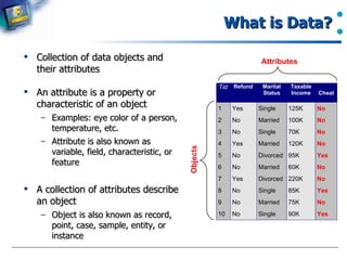
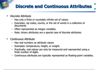


![Data Transformation : Normalization Min-max normalization: to [new_min A , new_max A ] Ex. Let income range $12,000 to $98,000 normalized to [0.0, 1.0]. Then $73,000 is mapped to Z-score normalization ( μ : mean, σ : standard deviation): Ex. Let μ = 54,000, σ = 16,000. Then Normalization by decimal scaling Where j is the smallest integer such that Max(| ν ’ |) < 1](https://image.slidesharecdn.com/ch-2-datapreprocessing-090808113508-phpapp01/85/Data-Preprocessing-25-320.jpg)


![Introduction to Data Mining Ch. 2 Data Preprocessing Heon Gyu Lee ( [email_address] ) http://dblab.chungbuk.ac.kr/~hglee DB/Bioinfo., Lab. http://dblab.chungbuk.ac.kr Chungbuk National University](https://image.slidesharecdn.com/ch-2-datapreprocessing-090808113508-phpapp01/75/Data-Preprocessing-1-2048.jpg)


![Data Transformation : Normalization Min-max normalization: to [new_min A , new_max A ] Ex. Let income range $12,000 to $98,000 normalized to [0.0, 1.0]. Then $73,000 is mapped to Z-score normalization ( μ : mean, σ : standard deviation): Ex. Let μ = 54,000, σ = 16,000. Then Normalization by decimal scaling Where j is the smallest integer such that Max(| ν ’ |) < 1](https://image.slidesharecdn.com/ch-2-datapreprocessing-090808113508-phpapp01/75/Data-Preprocessing-25-2048.jpg)


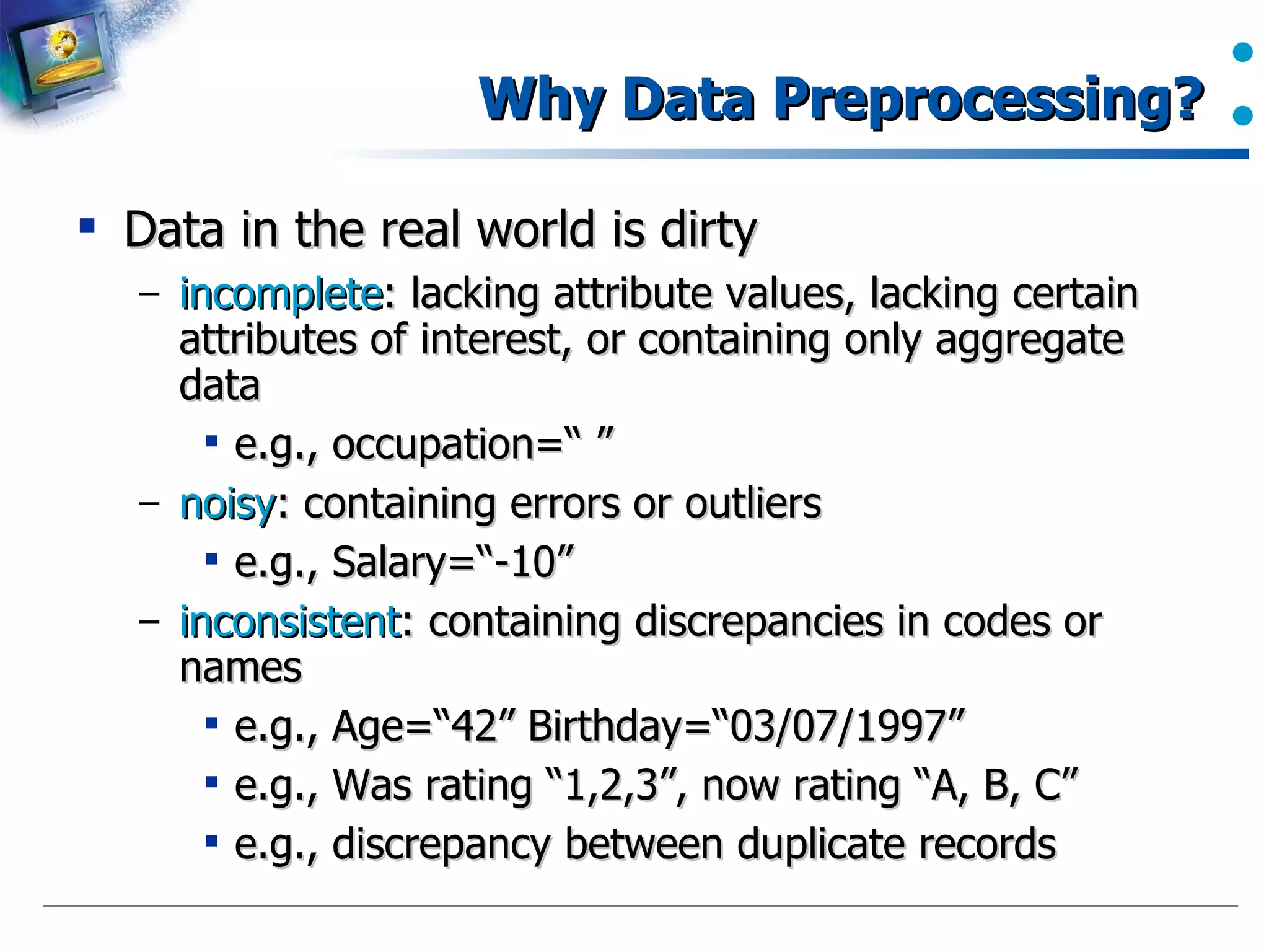
The document introduces data preprocessing techniques for data mining. It discusses why data preprocessing is important due to real-world data often being dirty, incomplete, noisy, inconsistent or duplicate. It then describes common data types and quality issues like missing values, noise, outliers and duplicates. The major tasks of data preprocessing are outlined as data cleaning, integration, transformation and reduction. Specific techniques for handling missing values, noise, outliers and duplicates are also summarized.
Overview of Data Mining and Preprocessing basics presented by Heon Gyu Lee from Chungbuk National University.
Data preprocessing is crucial due to the presence of dirty, incomplete, noisy, and inconsistent data in the real world.
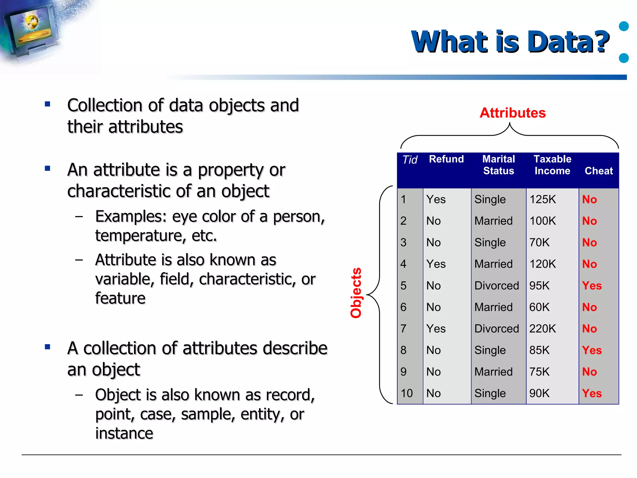
Definition of data, attributes, and their significance. Attributes may also be referred to as variables or features.
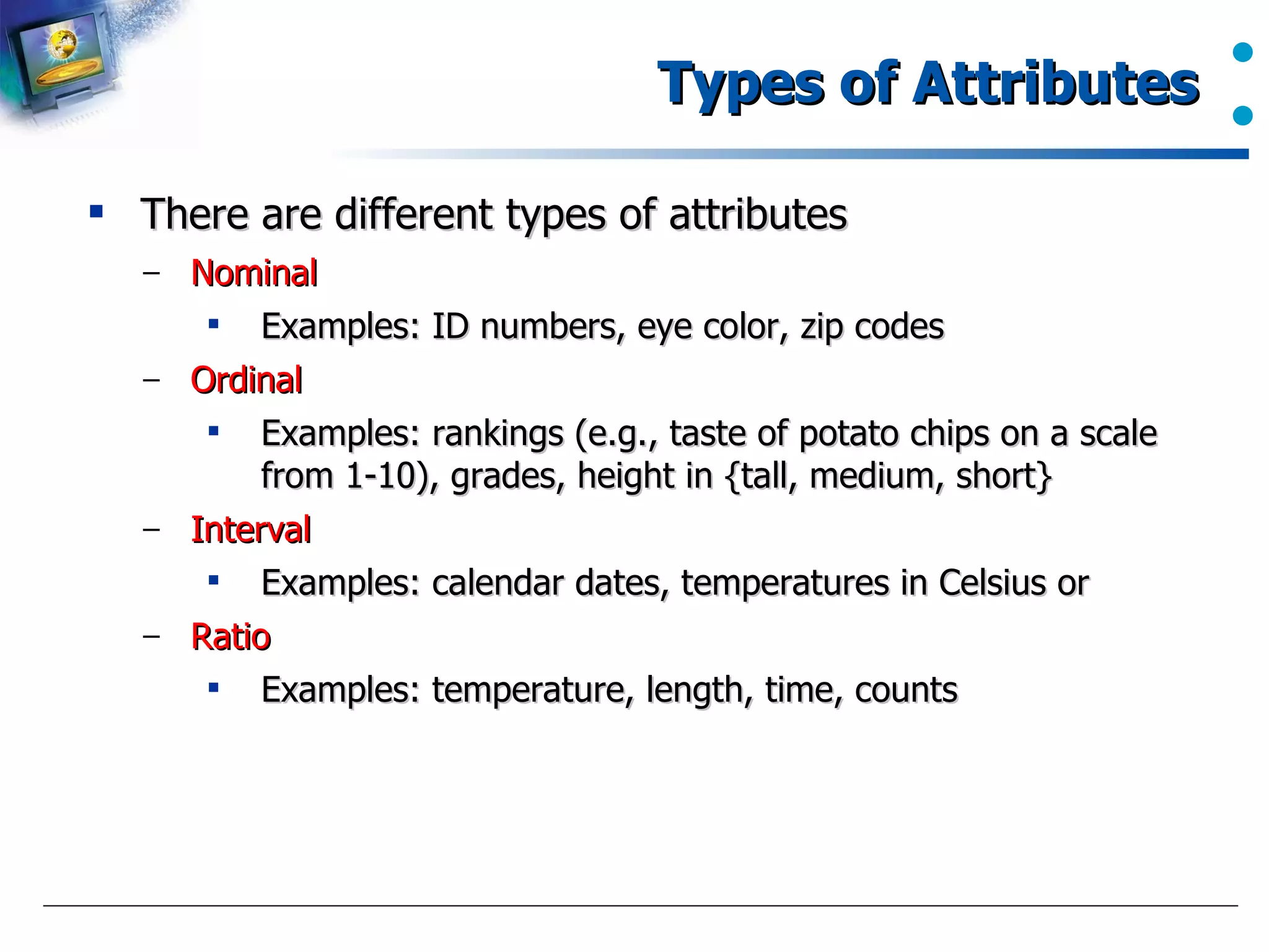
Different types of attributes such as nominal, ordinal, interval, and ratio with examples.
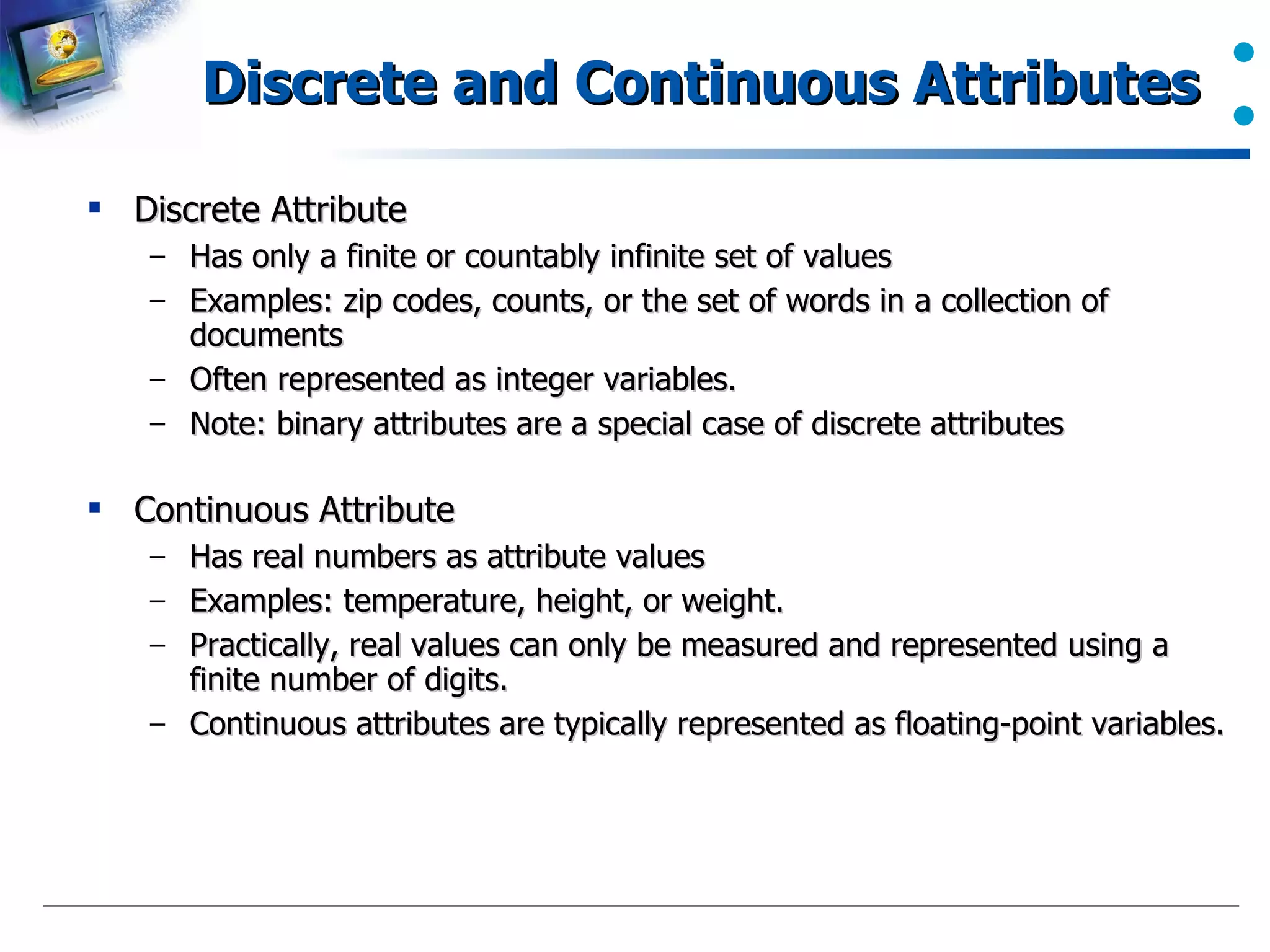
Explanation of discrete and continuous attributes, their representations, and examples.
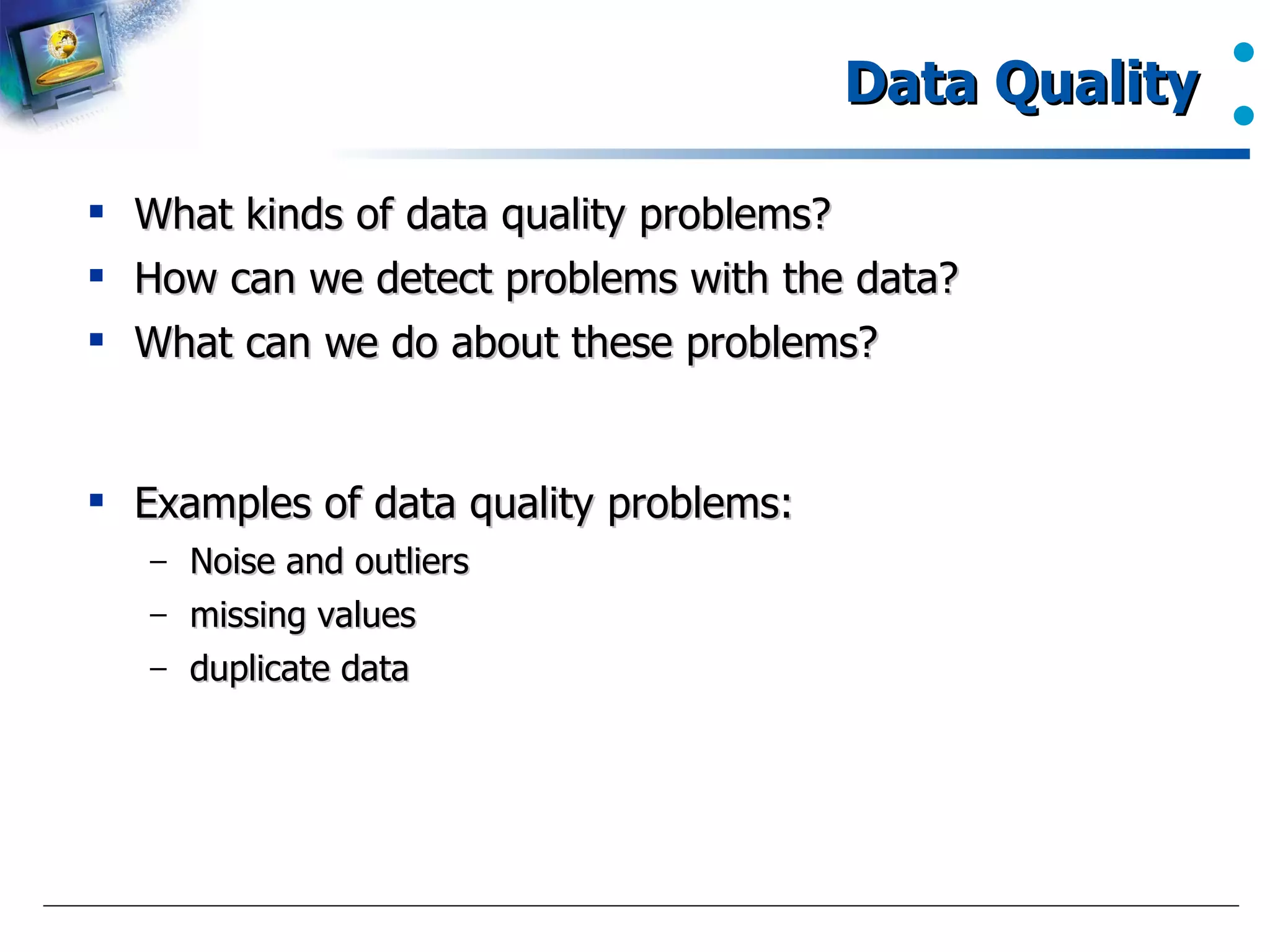
Key data quality problems include noise, outliers, missing values, and duplicates.
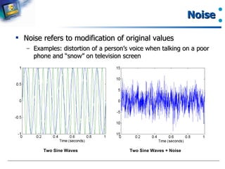
Definition of noise and its effect on data integrity with examples.
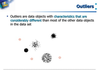
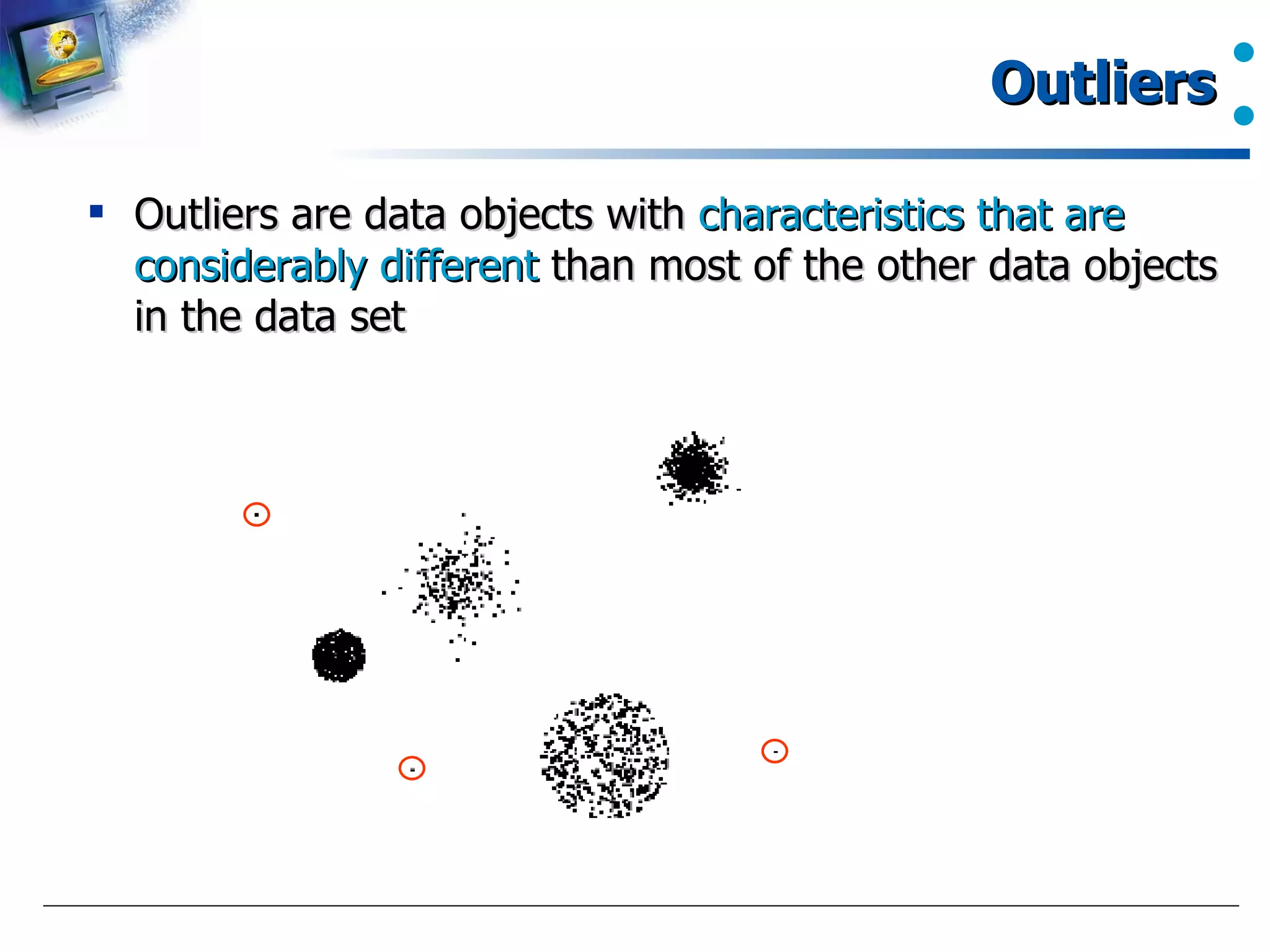
Outliers defined as data points deviating significantly from other observations in a dataset.
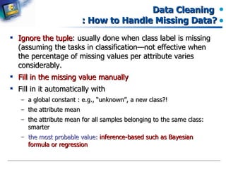
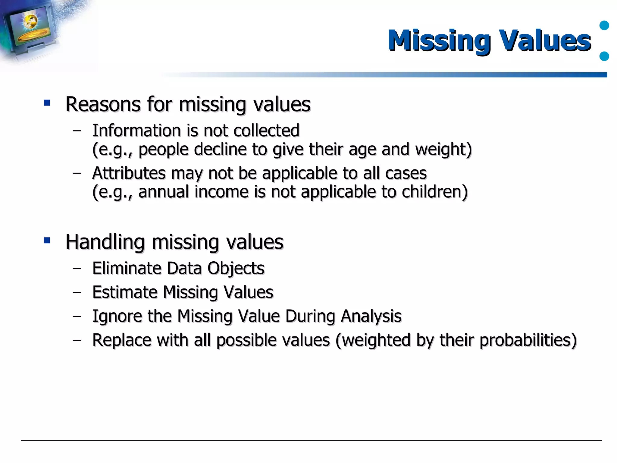
Reasons for missing values and methods for handling them, including deletion, estimation, and ignoring.
Challenges posed by duplicate data in datasets, particularly during integration from multiple sources.
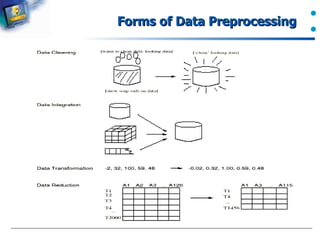
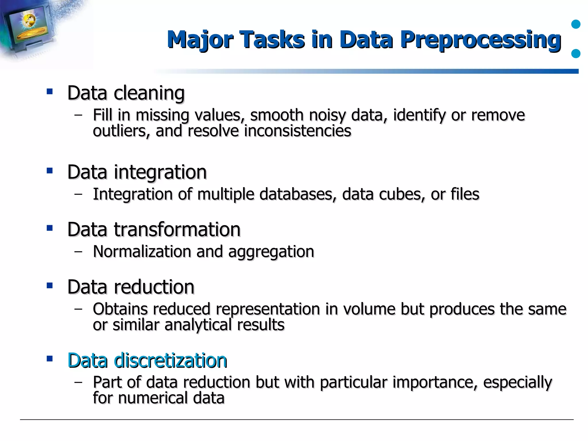
Data preprocessing tasks include cleaning, integration, transformation, and reduction.
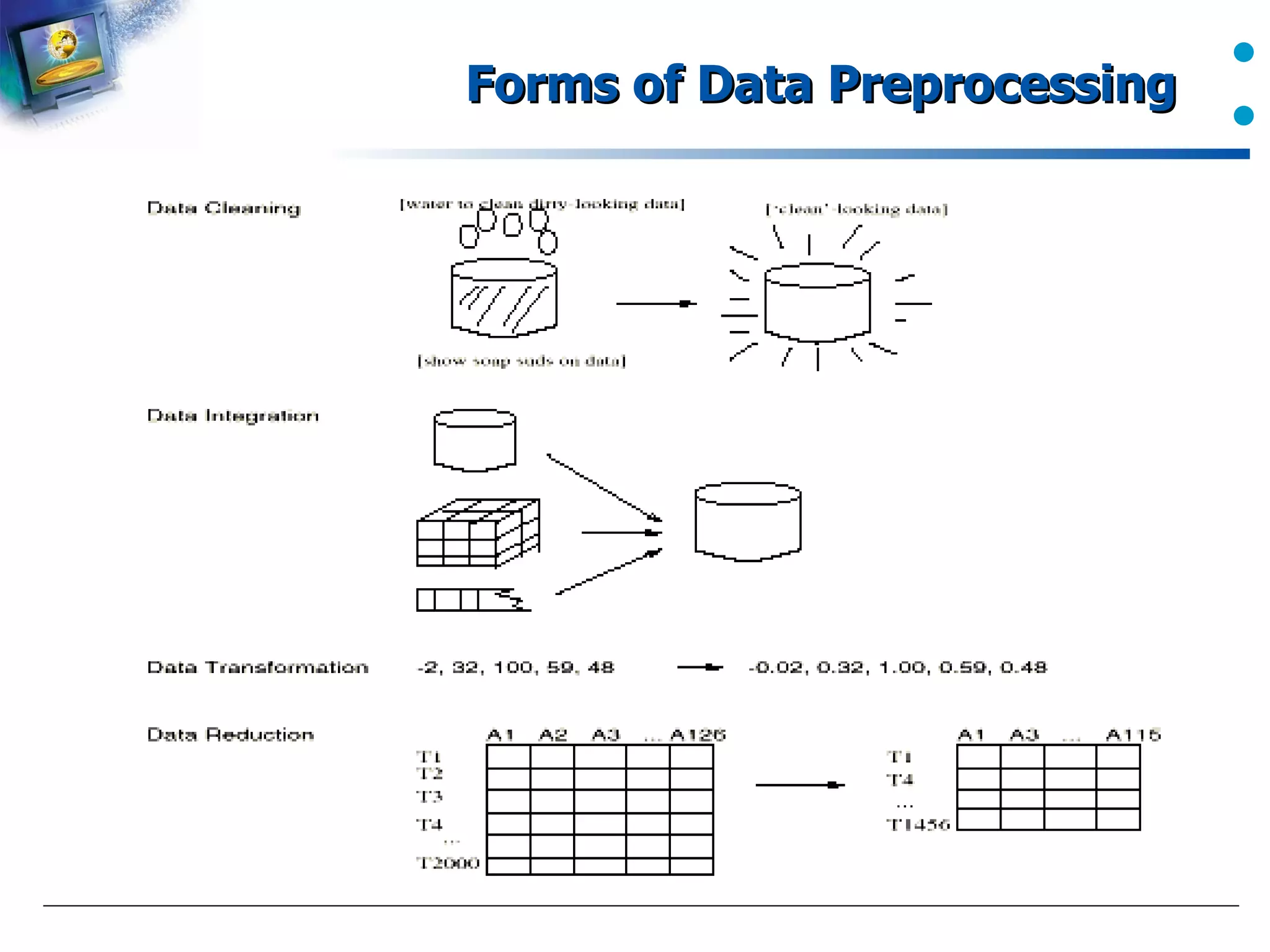
Forms of data preprocessing mentioned but specifics not detailed.
Highlighting the importance of data cleaning in data warehousing, citing expert opinions.
Various strategies for managing missing data effectively during analysis.
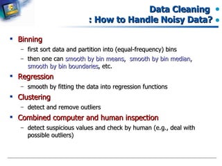
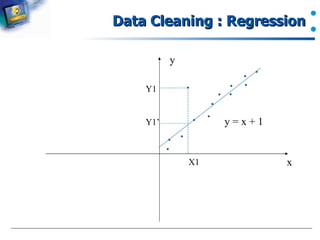
Methods for mitigating noise in data, including binning and regression.
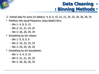
Describes the binning methods used for smoothing data during preprocessing.
Introduction to using regression analysis to manage noisy data.
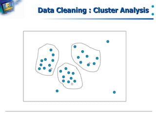
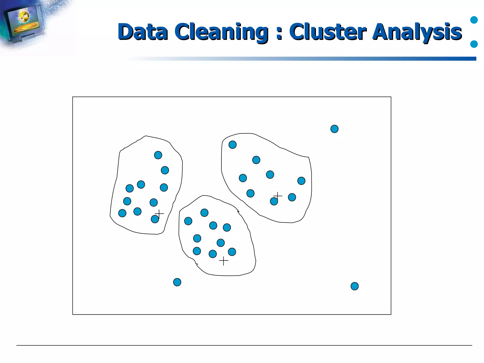
Use of cluster analysis as a technique in the context of data cleaning.
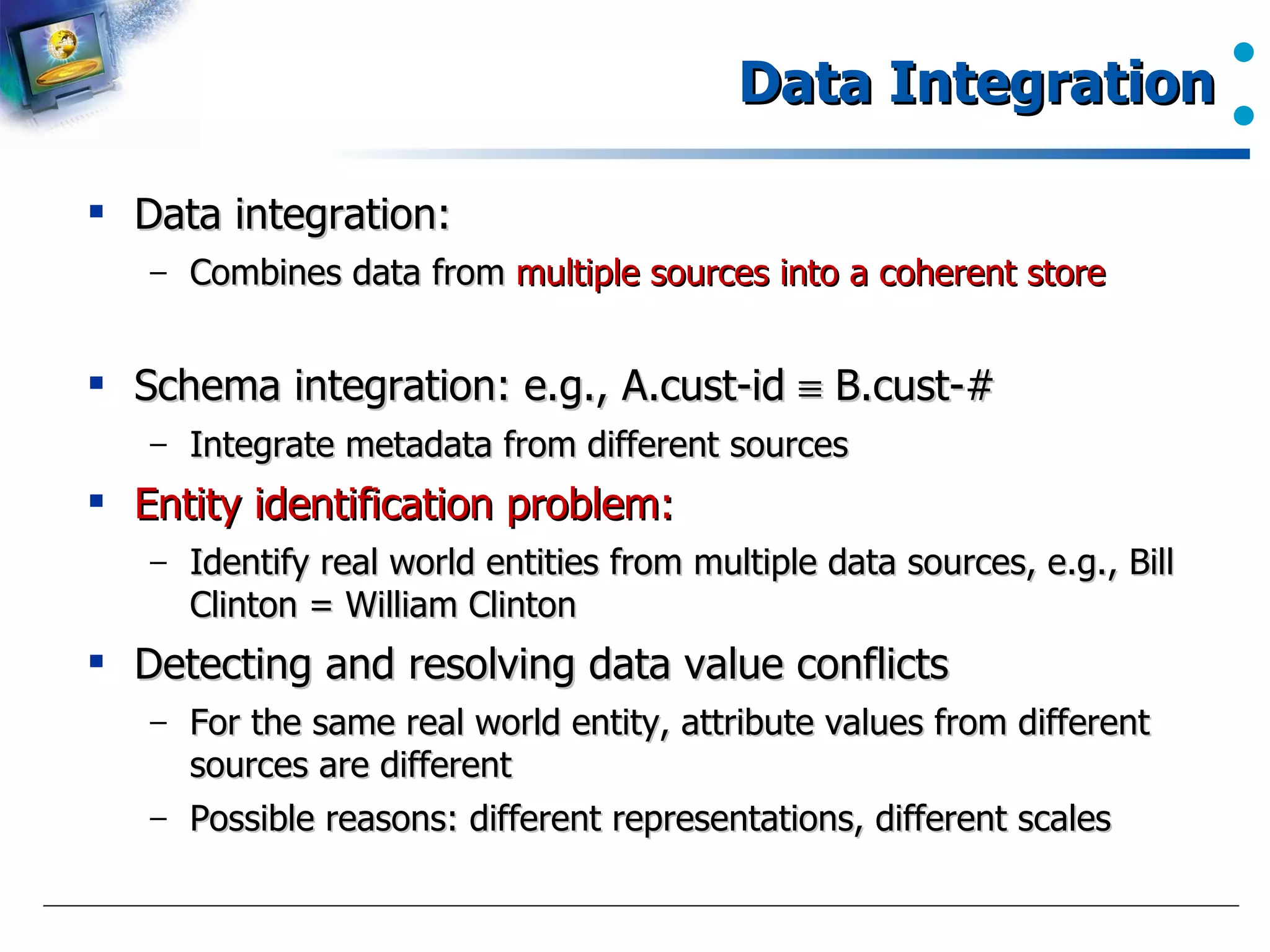
Explains data integration from multiple sources and identifying metadata conflicts.
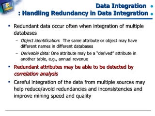
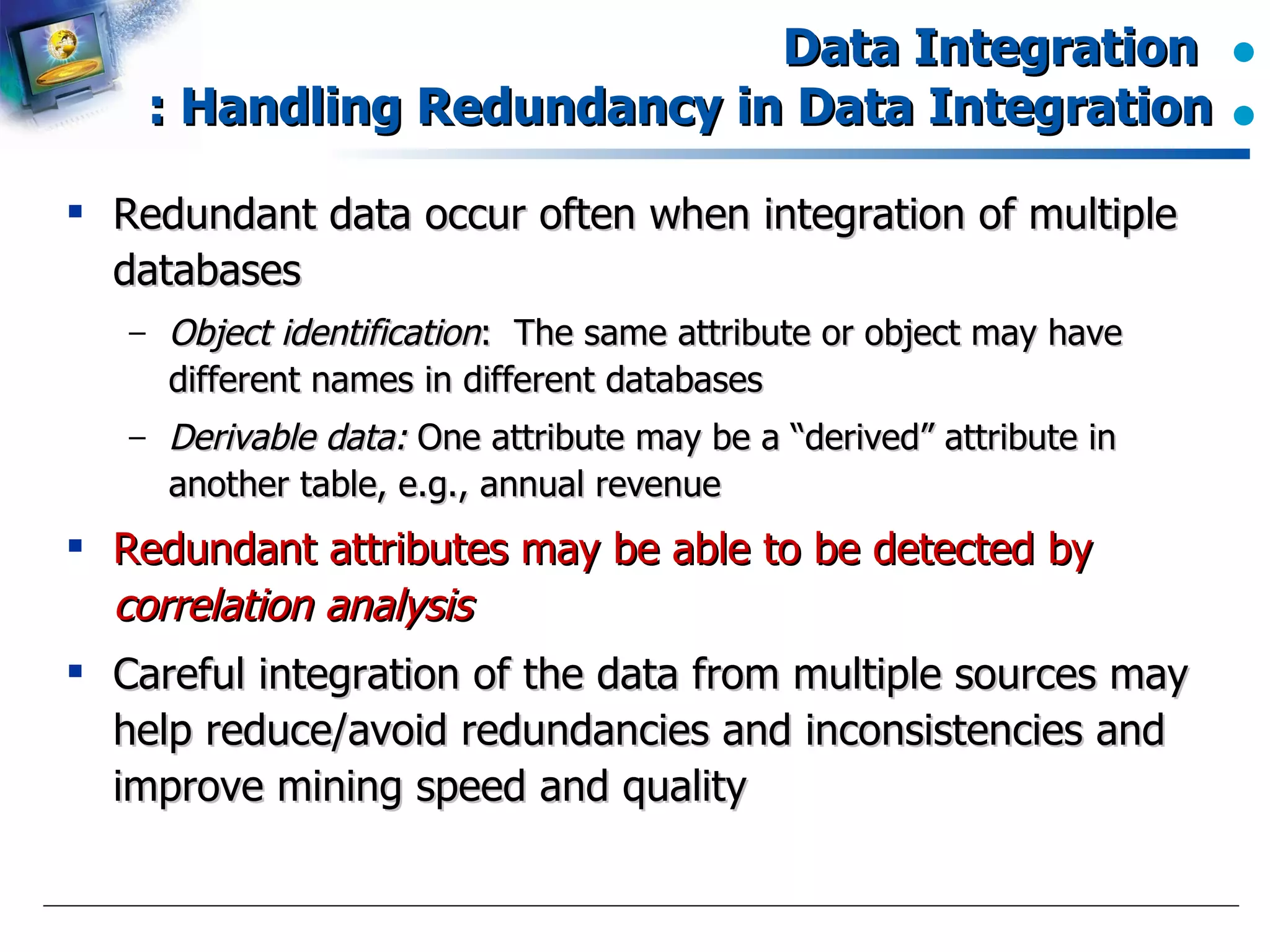
Discusses redundancy issues and solutions during data integration.
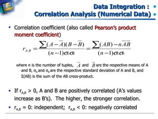
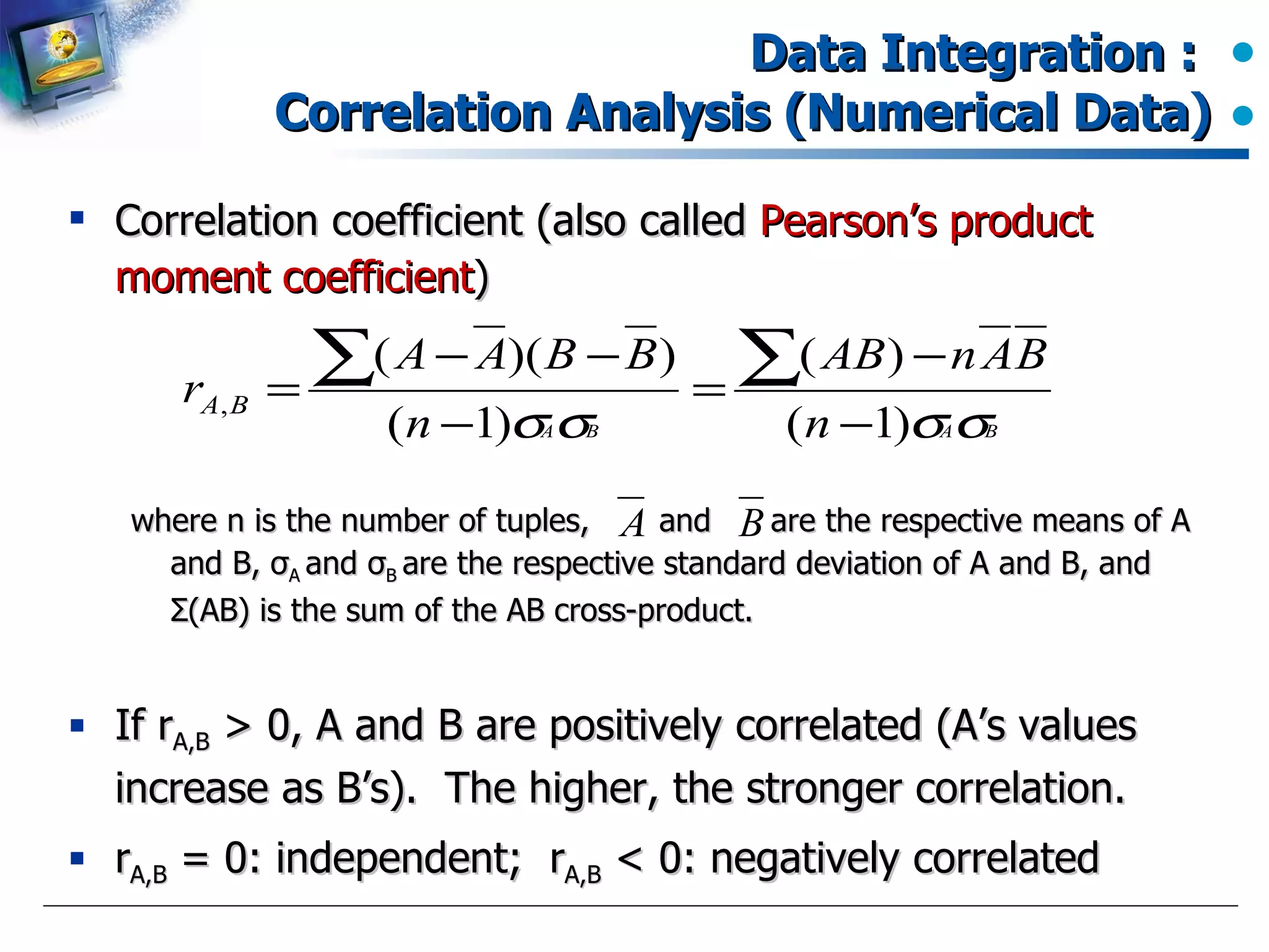
How correlation coefficients assess relationships between numerical attributes.
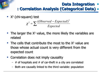
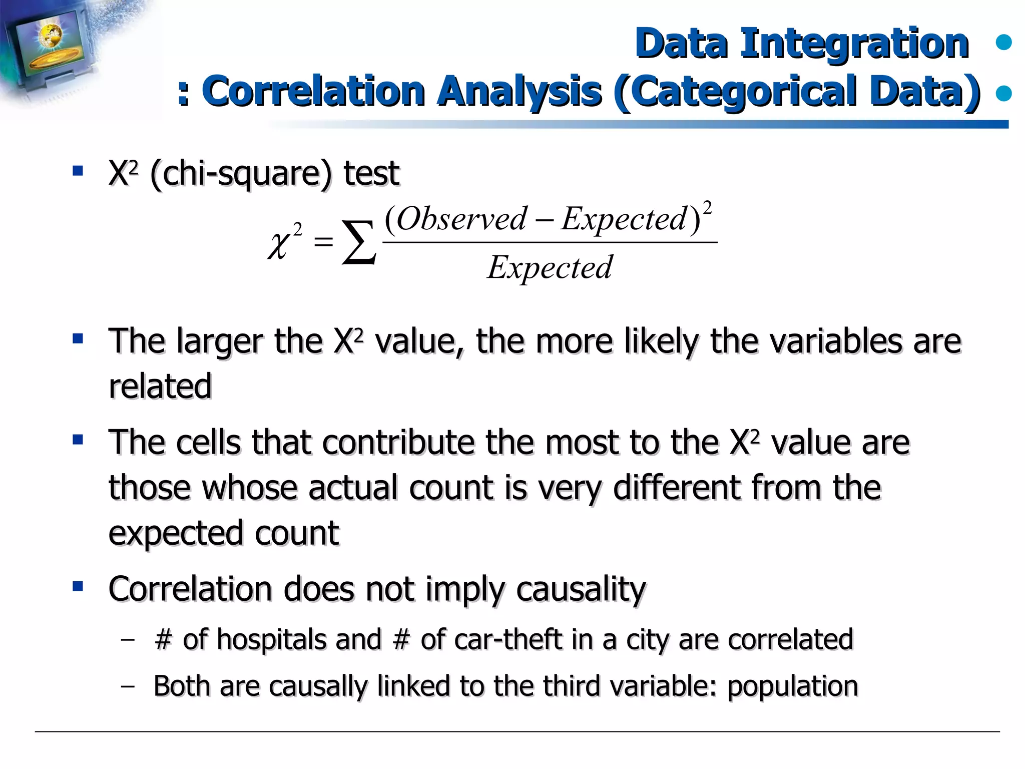
Application of chi-square tests in assessing relationships in categorical data.
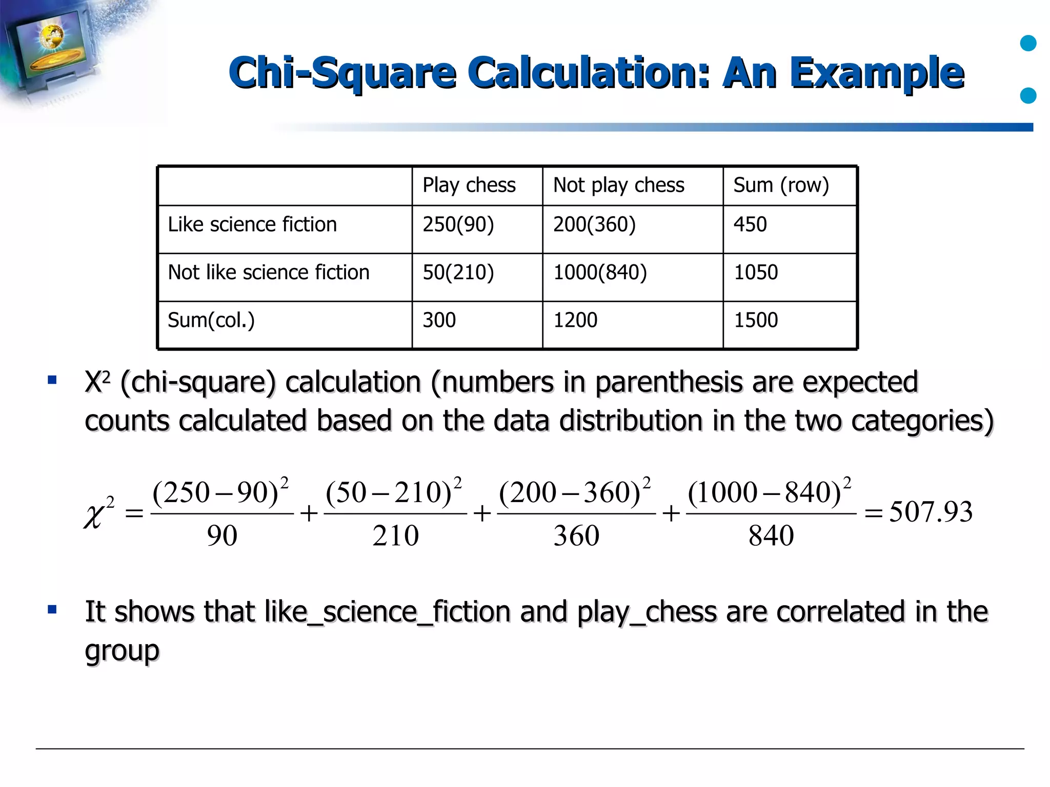
An example calculation of chi-square to demonstrate correlation in data.
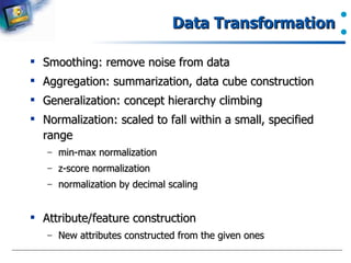
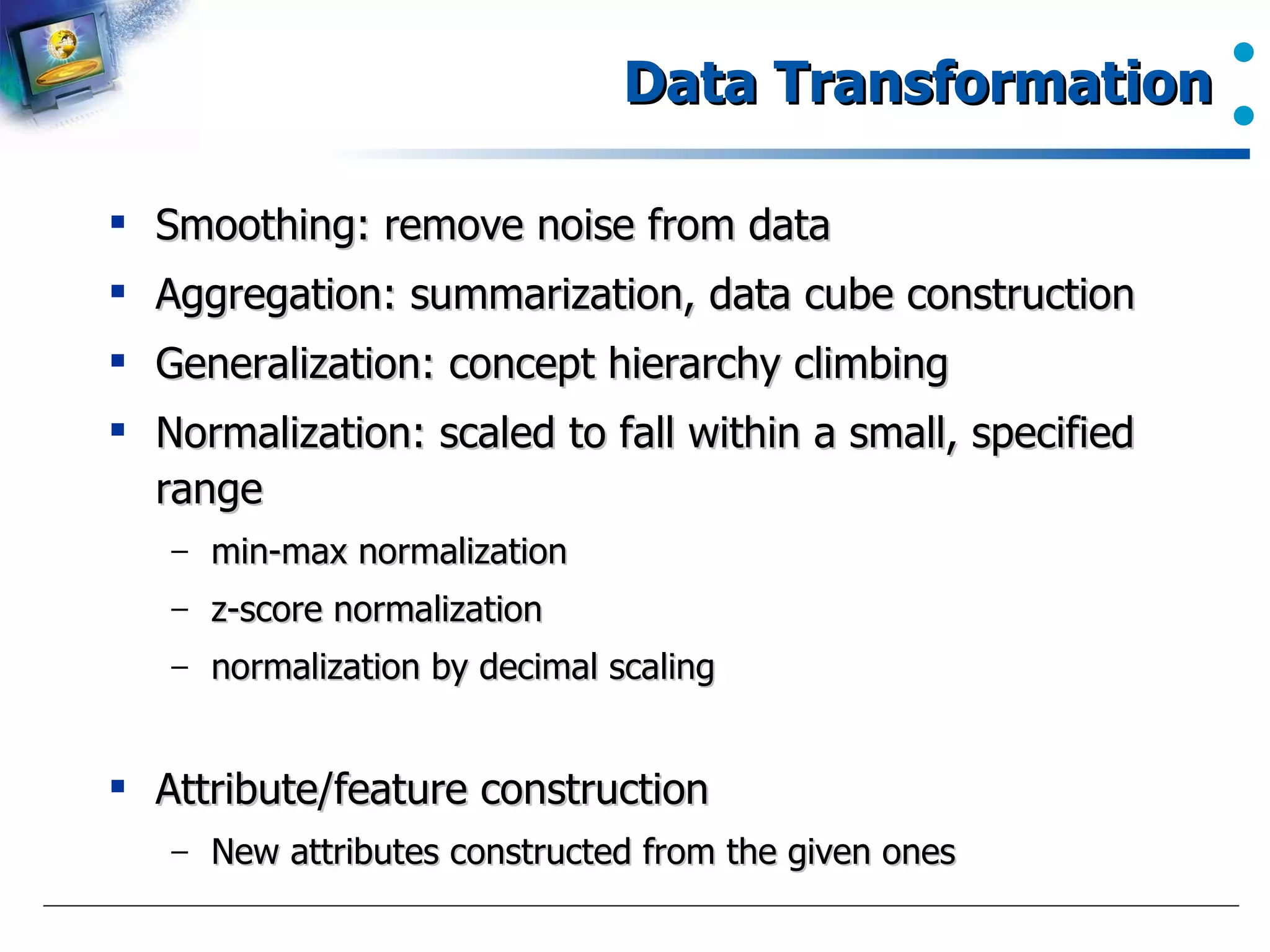
Various data transformation techniques used in preprocessing for improving data quality.
Methods for normalization such as min-max and z-score normalization.
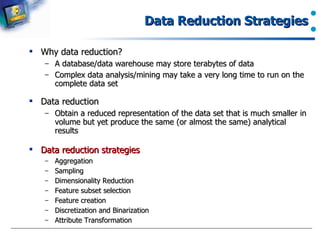
Reasons for data reduction to manage large datasets effectively.
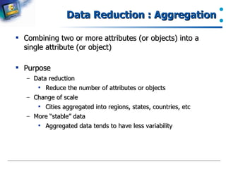
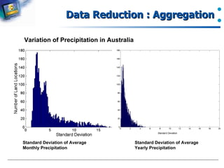
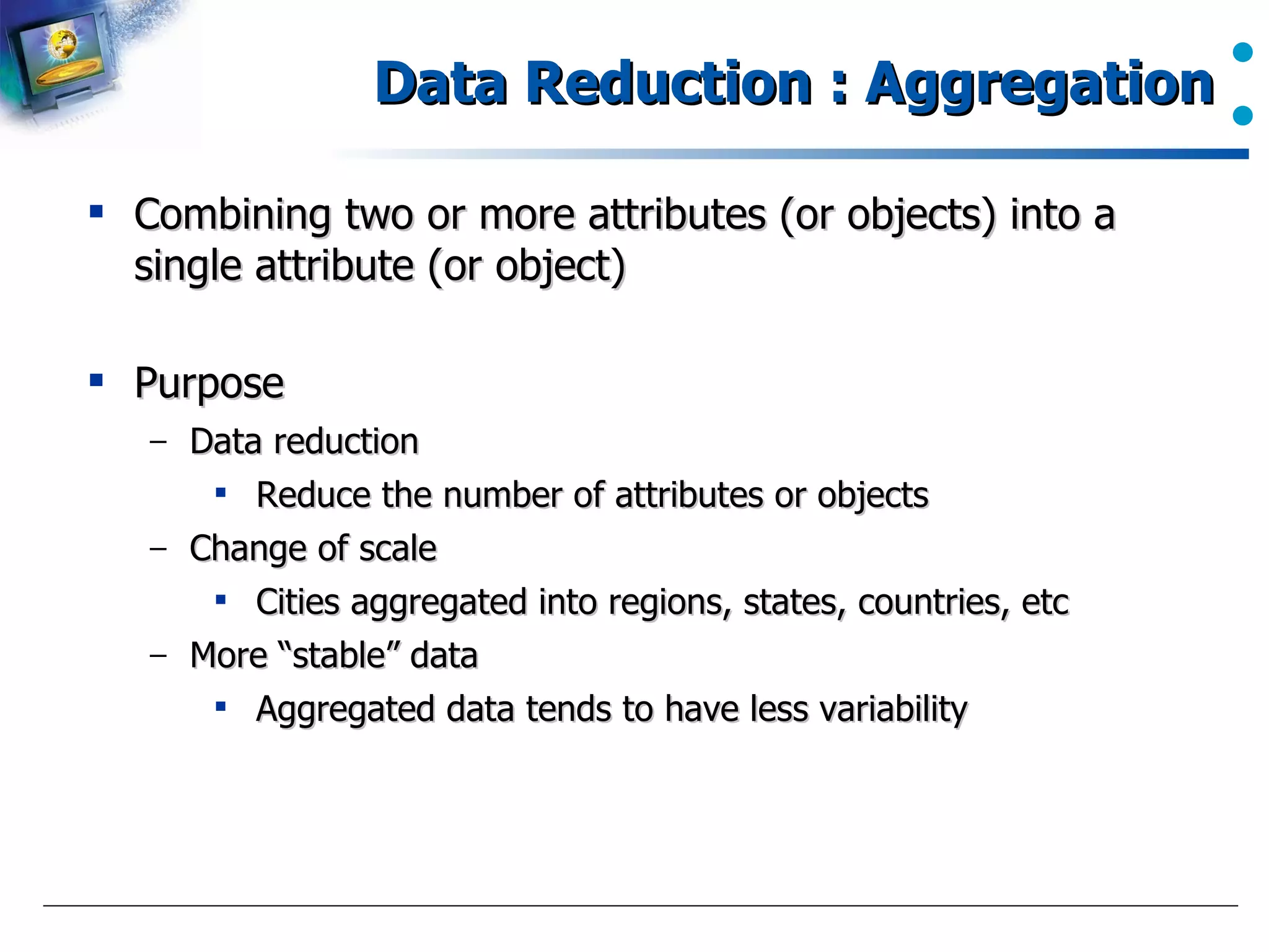
Describes the aggregation method for reducing data dimensions and variability.
Standard deviation calculations of aggregated precipitation data.
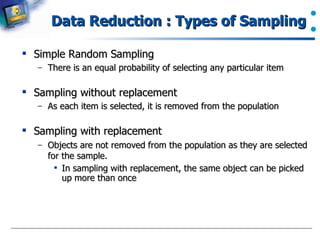
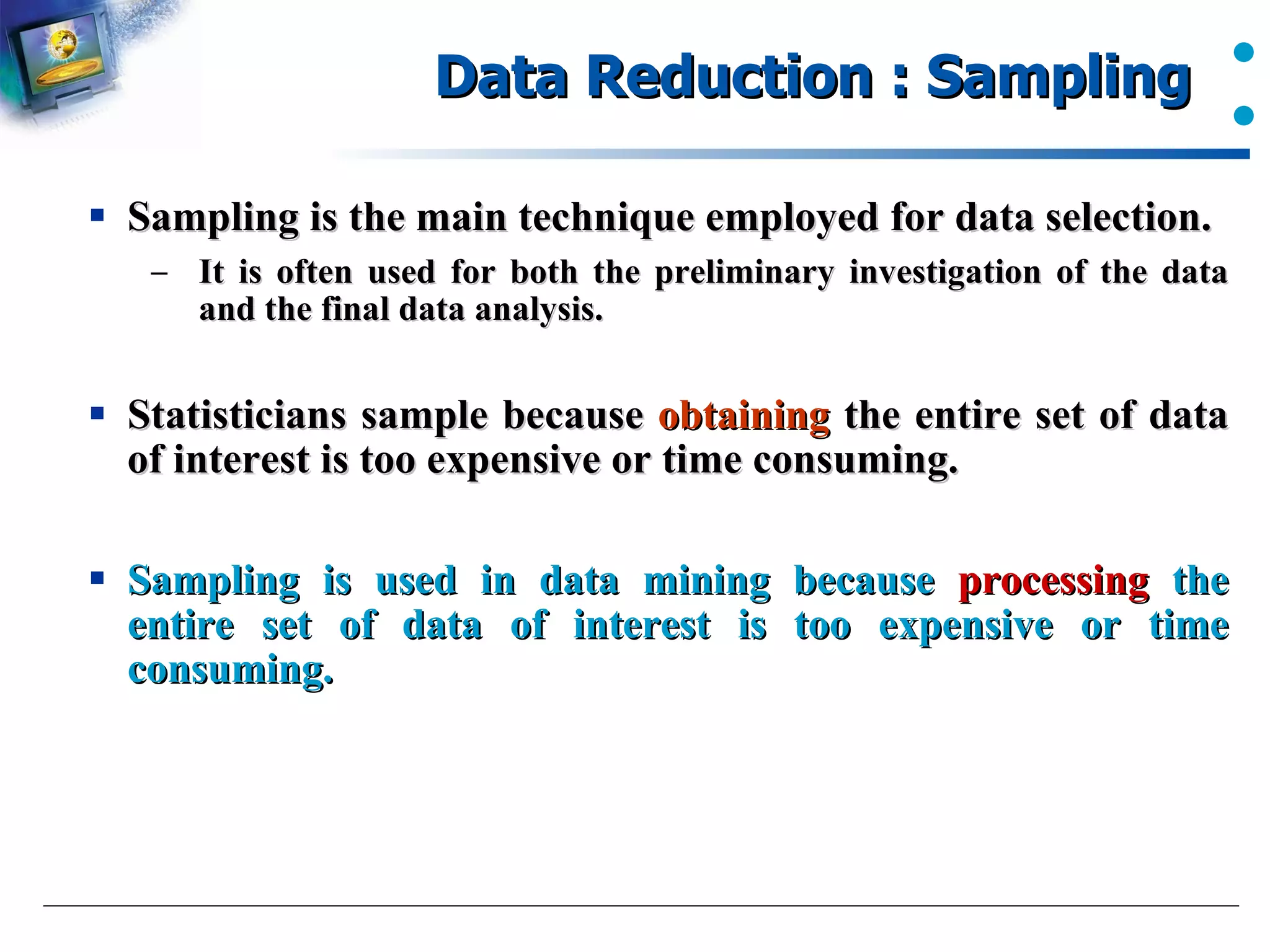
Sampling as a primary technique for data selection, its importance, and applications.
Different sampling methods: with and without replacement.
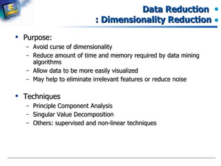
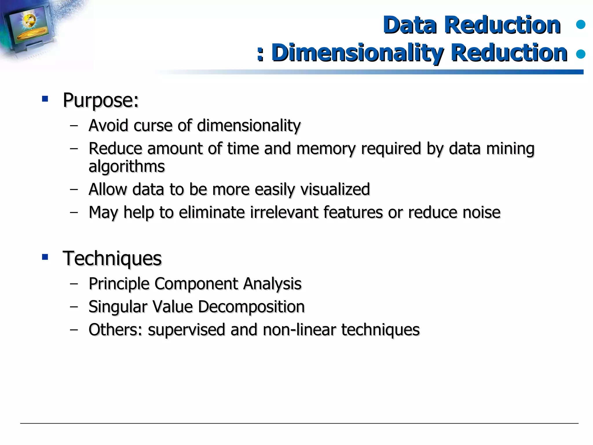
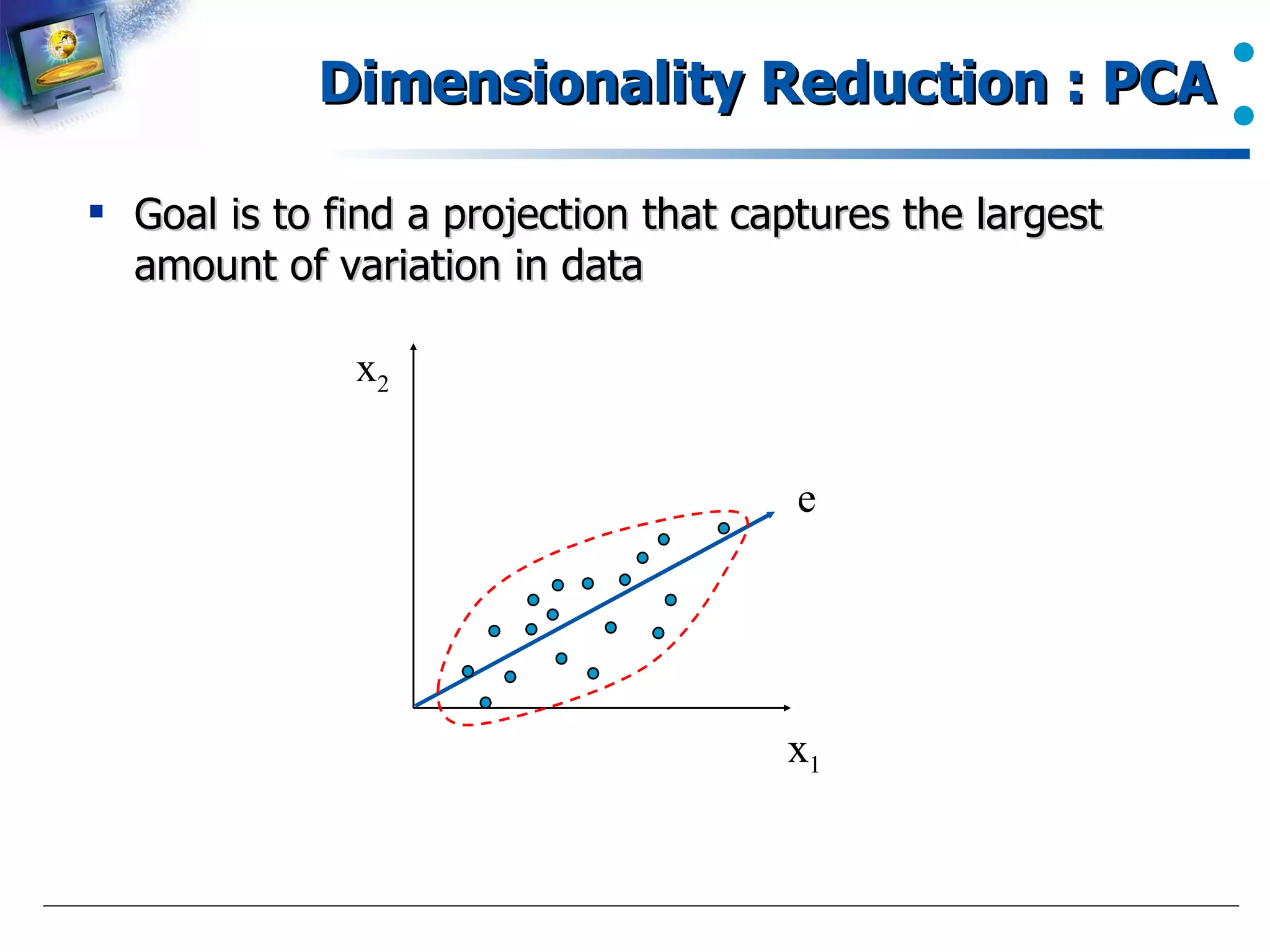
Purpose and benefits of dimensionality reduction in data analysis.
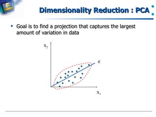
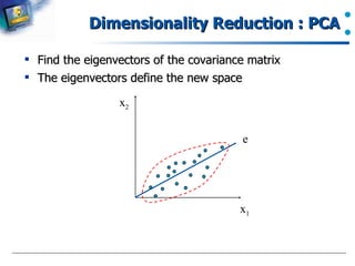
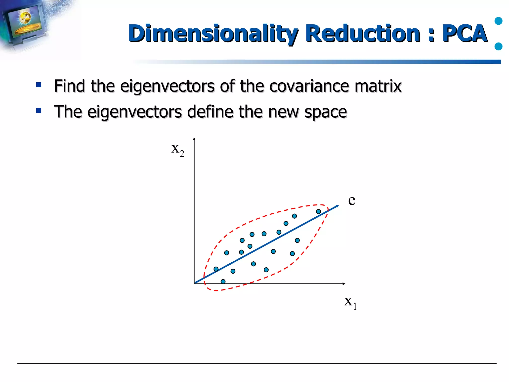
Introduction to PCA and its role in data dimensionality reduction.
A brief description of finding eigenvectors in PCA for transforming data.
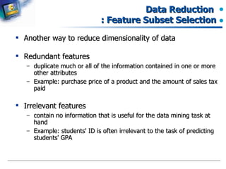
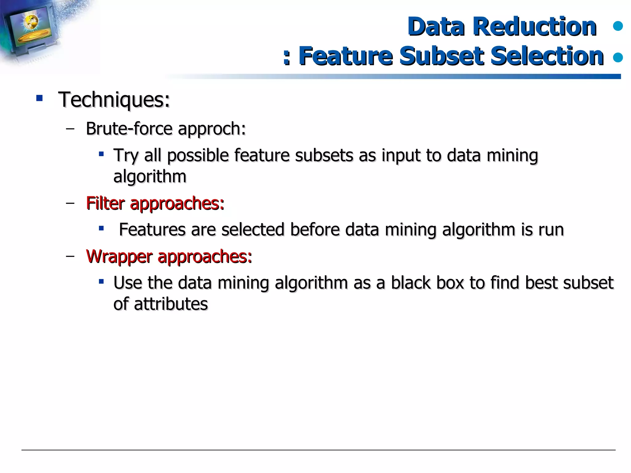
Methods for reducing dimensionality by selecting relevant features.
Various techniques for feature subset selection, including brute-force and filter approaches.
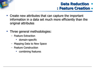
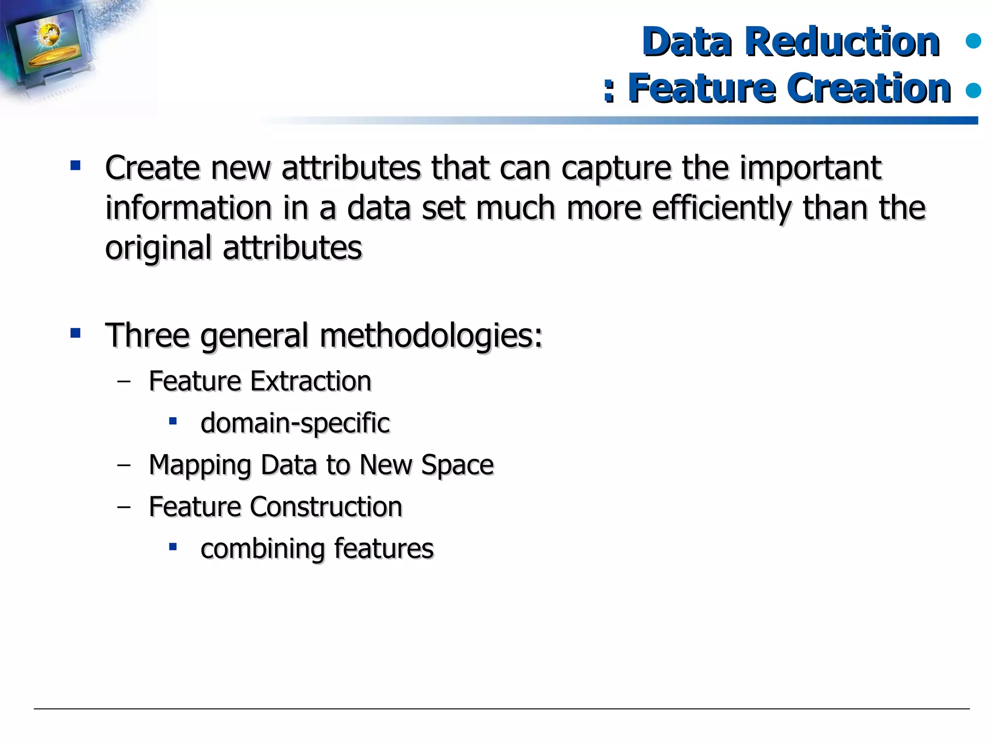
Methods of creating new attributes to improve data efficiency.
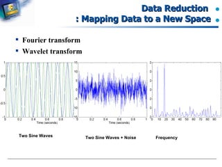
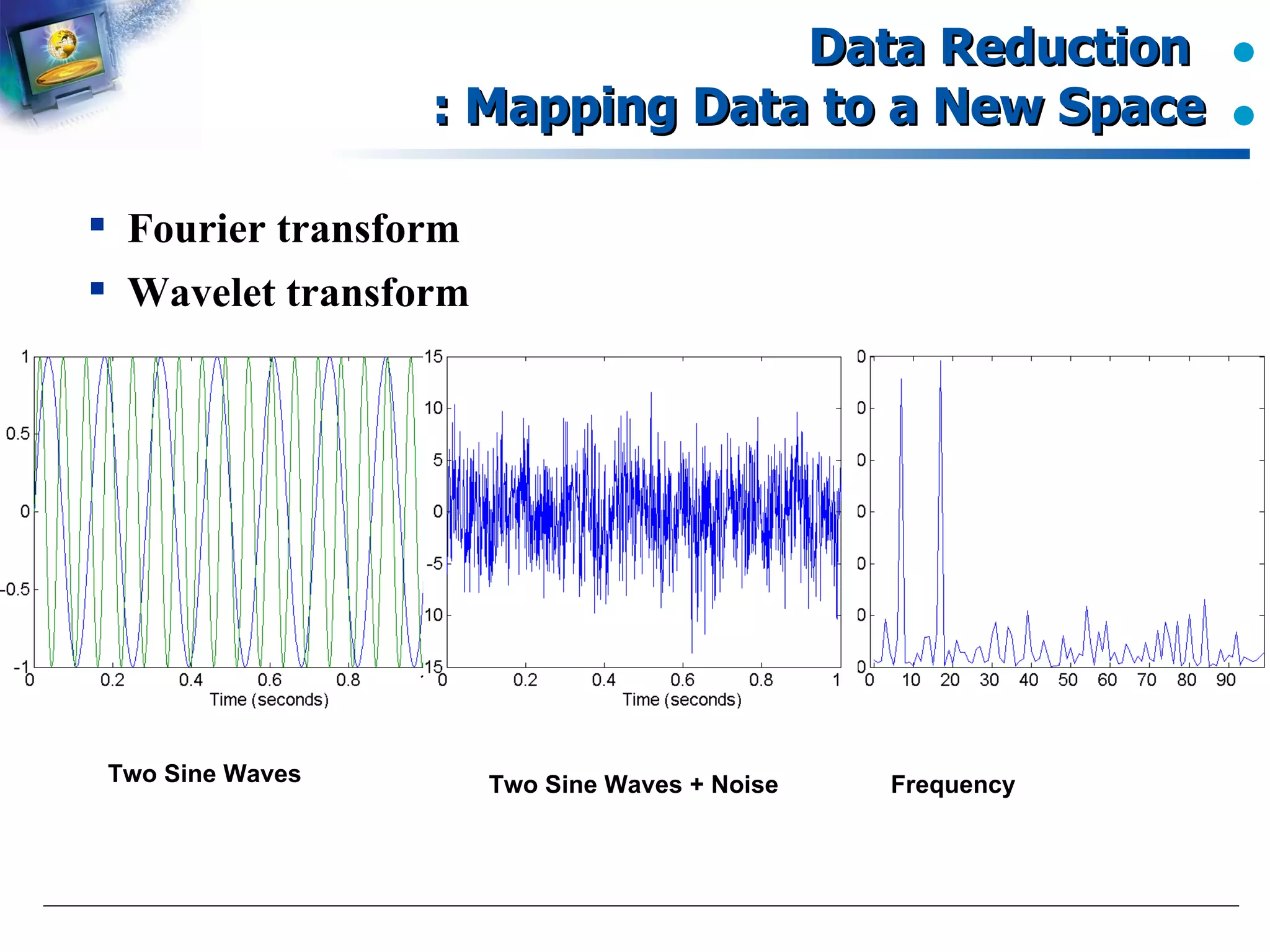
Description of methods like Fourier and Wavelet transforms.
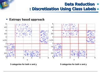
Entropy-based approaches for data discretization using class labels.
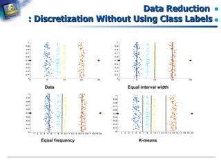
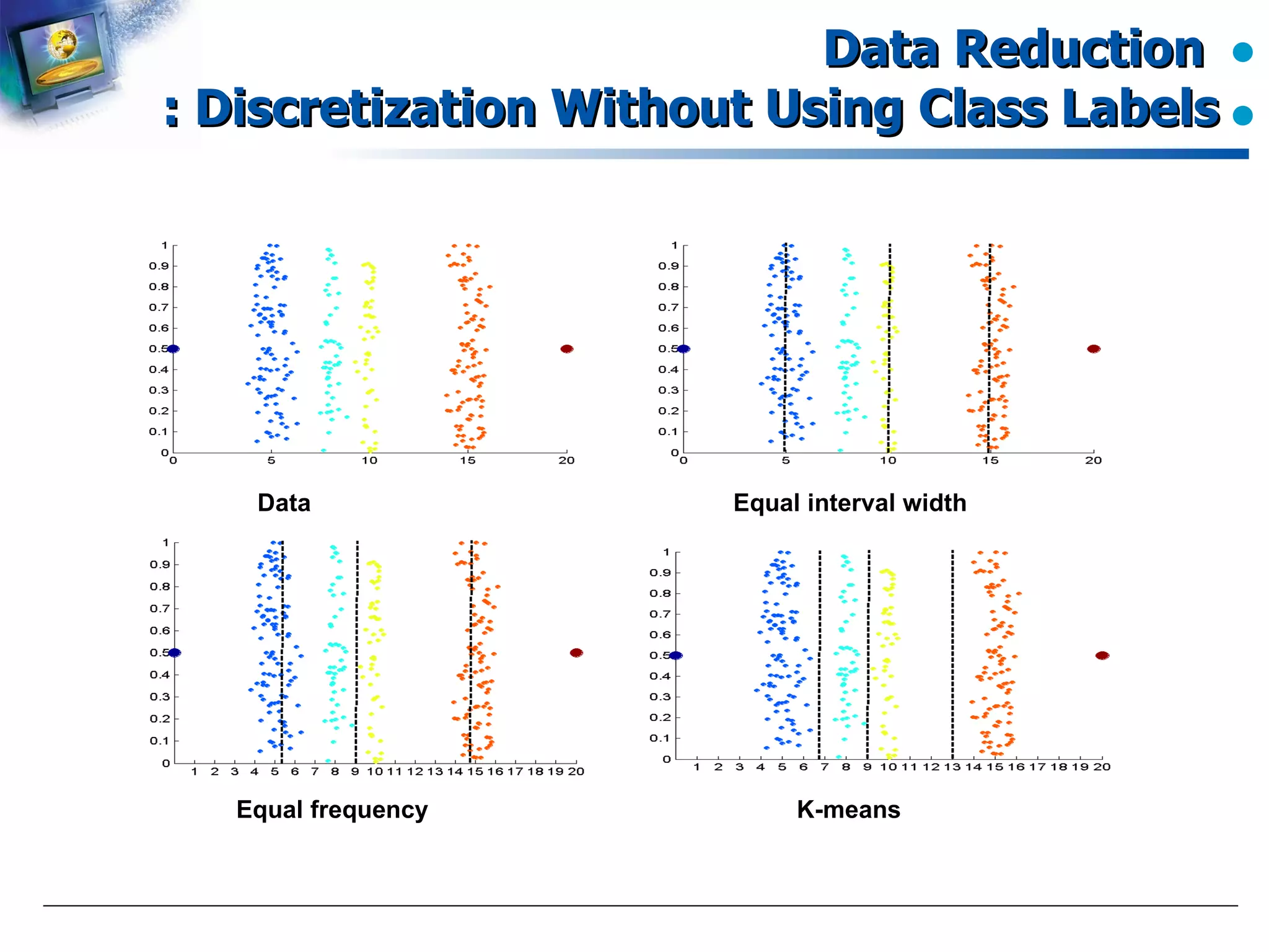
Various methods for discretization without using class labels.
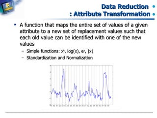
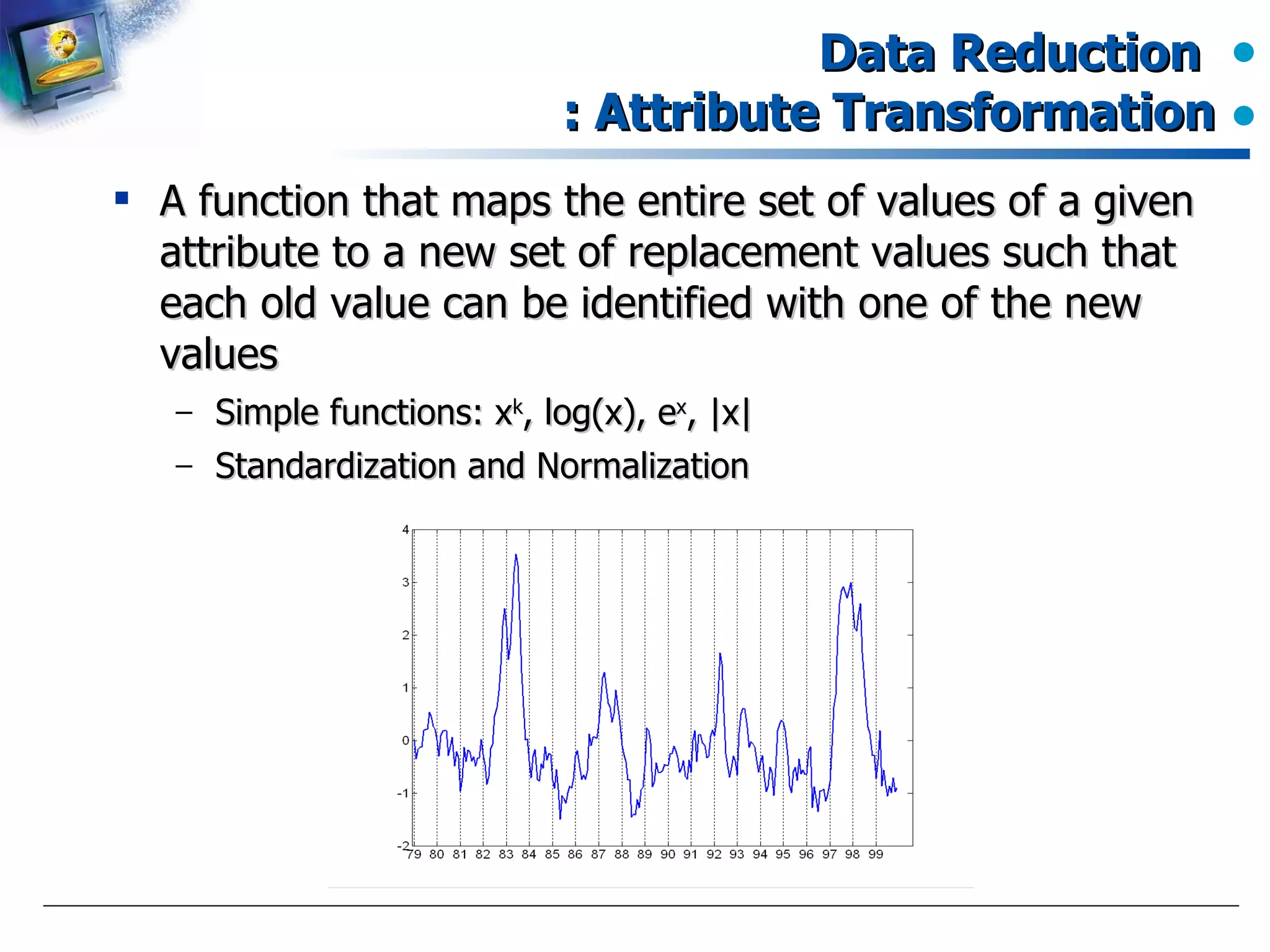
Functions for mapping attribute values to new representation during data preprocessing.
Closure of the presentation with a session for questions and answers.


