Data Strictures –Unit II
Part – 1 - Searching
Searching : basic searching techniques, sequential search,
binary search, iterative and recursive methods, comparison
between sequential and binary search.
2.
Searching: Introduction
• Searchingrefers to finding for an item in any list. It is one of the
common operations in data processing.
• Searching should be efficient and quick as the list may be large and
large amount of data has to be processed.
• The programmer has to select the best technique to the given
problem. Searching is made easy when the list is sorted.
3.
Basic Search Techniques
Thesearching technique that is being followed in the data structure is
listed below:
• 1. Linear Search or Sequential Search
• 2. Binary Search
4.
• Linear Searchor Sequential Search: In this technique of searching,
the element to be found in searching the elements to be found is
searched sequentially in the list.
• This method can be performed on a sorted or an unsorted list (usually
arrays).
• In case of a sorted list searching starts from 0th
element and continues
until the element is found from the list or the element whose value is
greater than (assuming the list is sorted in ascending order), the value
being searched is reached.
5.
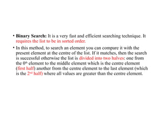
• Binary Search:It is a very fast and efficient searching technique. It
requires the list to be in sorted order.
• In this method, to search an element you can compare it with the
present element at the centre of the list. If it matches, then the search
is successful otherwise the list is divided into two halves: one from
the 0th
element to the middle element which is the centre element
(first half) another from the centre element to the last element (which
is the 2nd
half) where all values are greater than the centre element.
6.
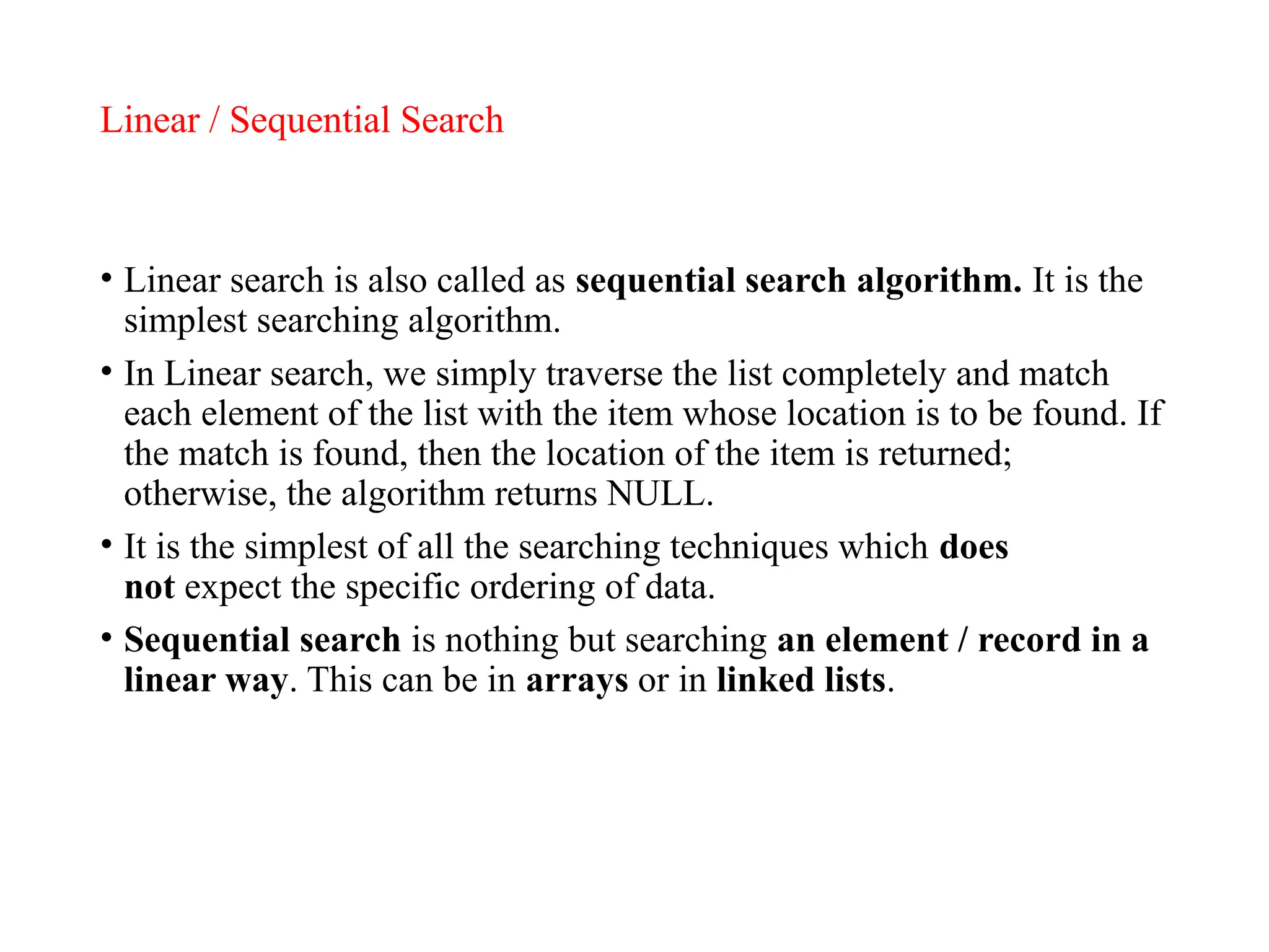
Linear / SequentialSearch
• Linear search is also called as sequential search algorithm. It is the
simplest searching algorithm.
• In Linear search, we simply traverse the list completely and match
each element of the list with the item whose location is to be found. If
the match is found, then the location of the item is returned;
otherwise, the algorithm returns NULL.
• It is the simplest of all the searching techniques which does
not expect the specific ordering of data.
• Sequential search is nothing but searching an element / record in a
linear way. This can be in arrays or in linked lists.
7.
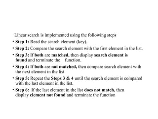
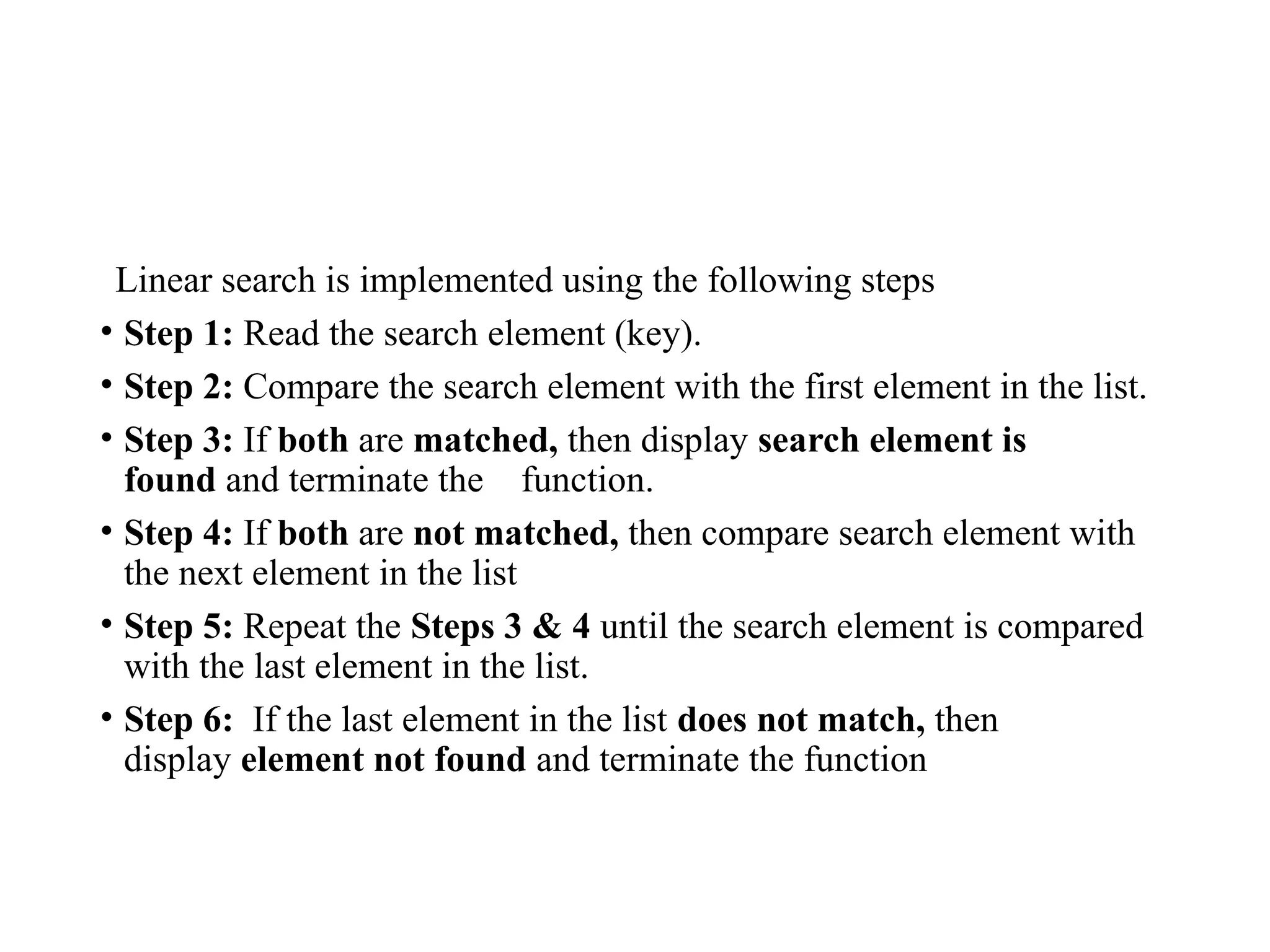
Linear search isimplemented using the following steps
• Step 1: Read the search element (key).
• Step 2: Compare the search element with the first element in the list.
• Step 3: If both are matched, then display search element is
found and terminate the function.
• Step 4: If both are not matched, then compare search element with
the next element in the list
• Step 5: Repeat the Steps 3 & 4 until the search element is compared
with the last element in the list.
• Step 6: If the last element in the list does not match, then
display element not found and terminate the function
8.
Algorithm: Linear Search
Algorithm:Linear Search (list [ ], n, key)
Let list [ ] be a linear array with n elements and key is an element to
be searched in the list
Step 1: Set i = 0
Step 2: while (i < n) do
If list [i] == key then
return i; //Key found at ith
location
end while
Step 3: return -1; //key not found
11.
Binary Search
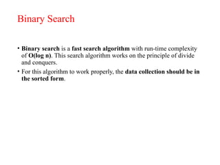
• Binarysearch is a fast search algorithm with run-time complexity
of Ο(log n). This search algorithm works on the principle of divide
and conquers.
• For this algorithm to work properly, the data collection should be in
the sorted form.
12.
Input: Given anarray A of n elements in sorted order and item is an element to be
searched.
Output: Returns the position of item element if successful and returns -1 otherwise,
Step 1: set first = 0, last = n – 1
Step 2: while (first <= last)
mid = (first + last) / 2
if (item == A[mid])
return (mid + 1);
else if (item < A[mid])
last = mid – 1
else
first = mid + 1
end while
Step 3: return -1
13.
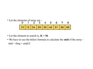
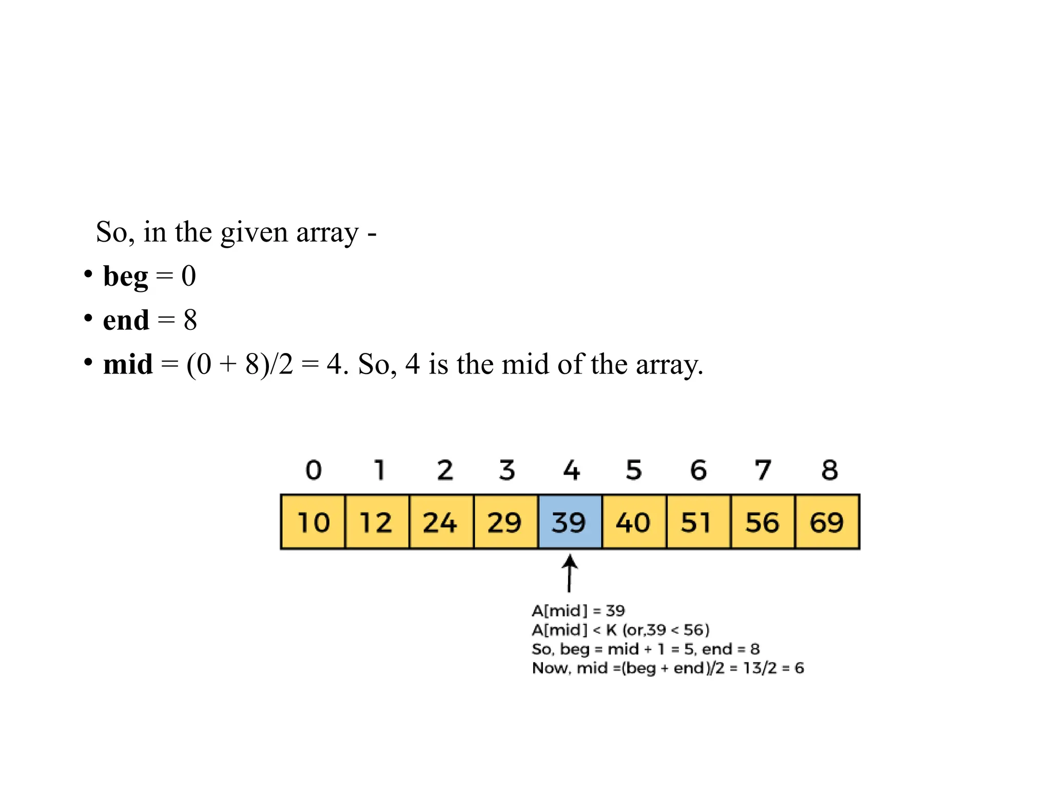
• Let theelements of array are –
• Let the element to search is, K = 56
• We have to use the below formula to calculate the mid of the array –
mid = (beg + end)/2
14.
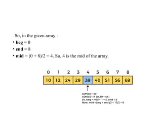
So, in thegiven array -
• beg = 0
• end = 8
• mid = (0 + 8)/2 = 4. So, 4 is the mid of the array.
15.
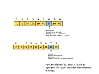
Now, the elementto search is found. So
algorithm will return the index of the element
matched.
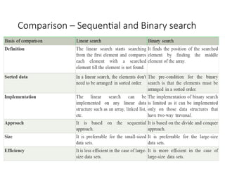
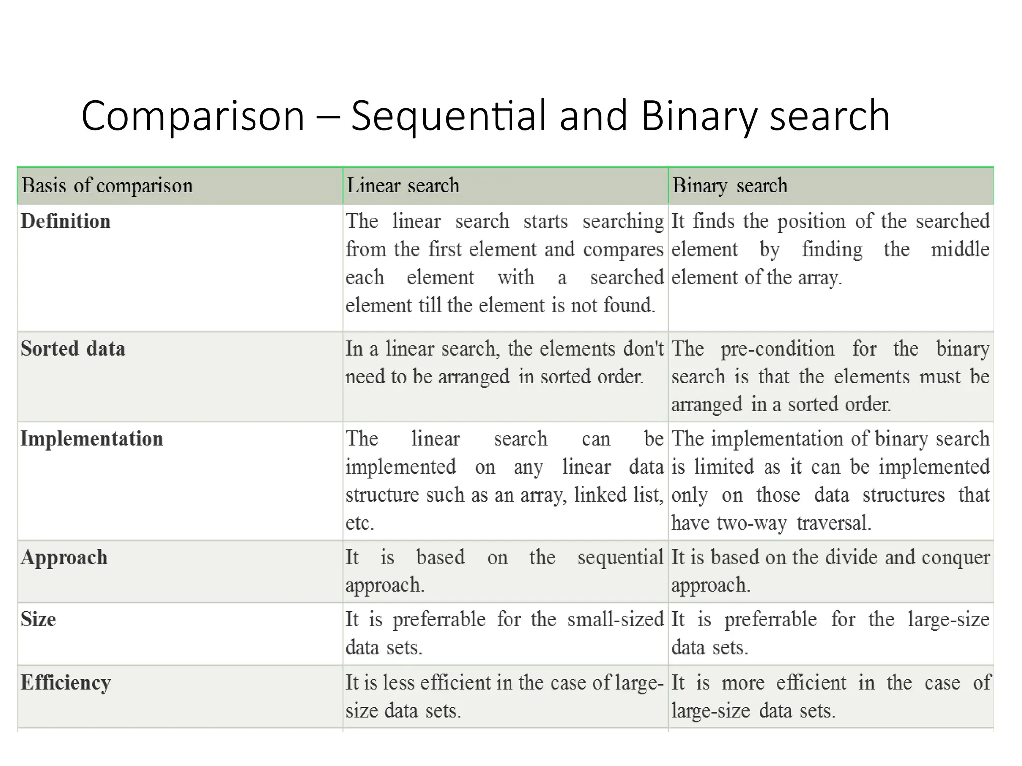
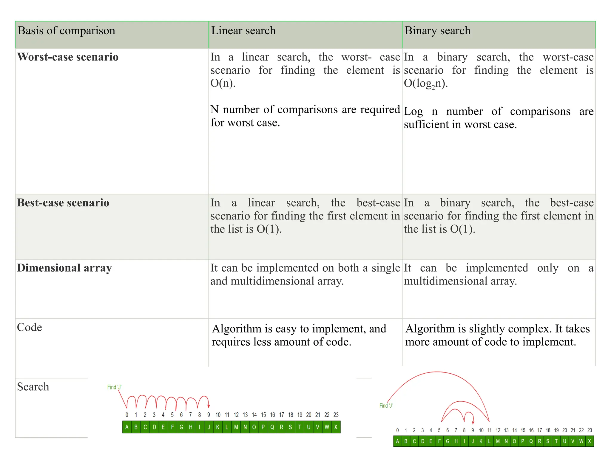
Basis of comparisonLinear search Binary search
Worst-case scenario In a linear search, the worst- case
scenario for finding the element is
O(n).
N number of comparisons are required
for worst case.
In a binary search, the worst-case
scenario for finding the element is
O(log2n).
Log n number of comparisons are
sufficient in worst case.
Best-case scenario In a linear search, the best-case
scenario for finding the first element in
the list is O(1).
In a binary search, the best-case
scenario for finding the first element in
the list is O(1).
Dimensional array It can be implemented on both a single
and multidimensional array.
It can be implemented only on a
multidimensional array.
Code Algorithm is easy to implement, and
requires less amount of code.
Algorithm is slightly complex. It takes
more amount of code to implement.
Search
18.
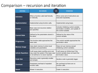
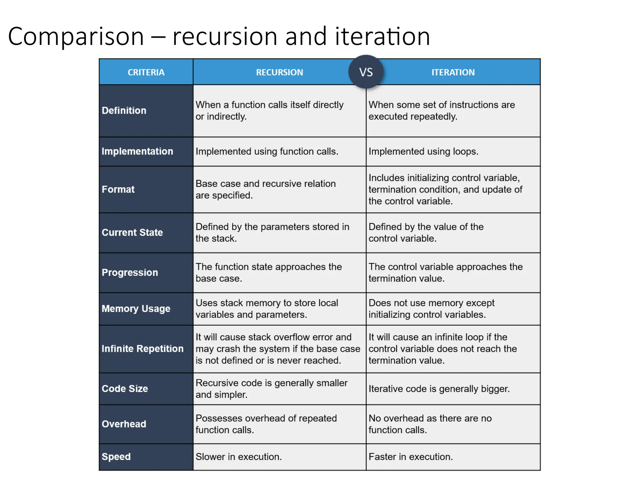
Iterative and Recursivemethods
• The Recursion and Iteration both repeatedly execute the set of
instructions.
• Recursion is when a statement in a function calls itself repeatedly.
The iteration is when a loop repeatedly executes until the
controlling condition becomes false.
• The primary difference between recursion and iteration is
that recursion is a process, always applied to a function
and iteration is applied to the set of instructions which we want to
get repeatedly executed.
19.
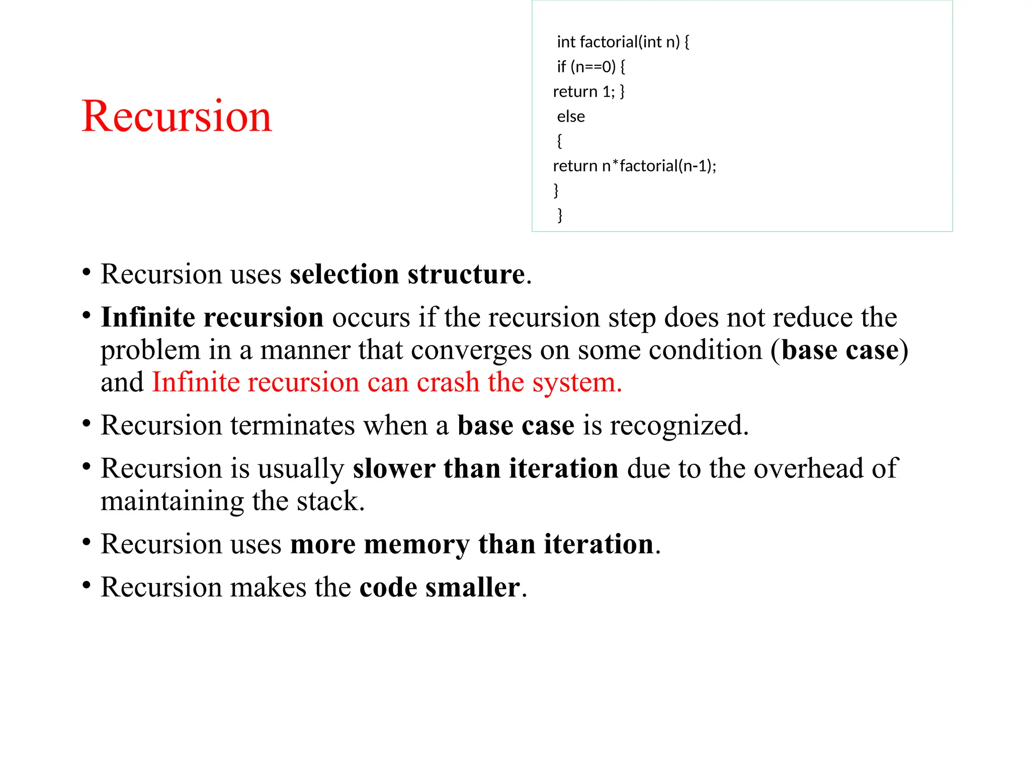
Recursion
• Recursion usesselection structure.
• Infinite recursion occurs if the recursion step does not reduce the
problem in a manner that converges on some condition (base case)
and Infinite recursion can crash the system.
• Recursion terminates when a base case is recognized.
• Recursion is usually slower than iteration due to the overhead of
maintaining the stack.
• Recursion uses more memory than iteration.
• Recursion makes the code smaller.
int factorial(int n) {
if (n==0) {
return 1; }
else
{
return n*factorial(n-1);
}
}
20.
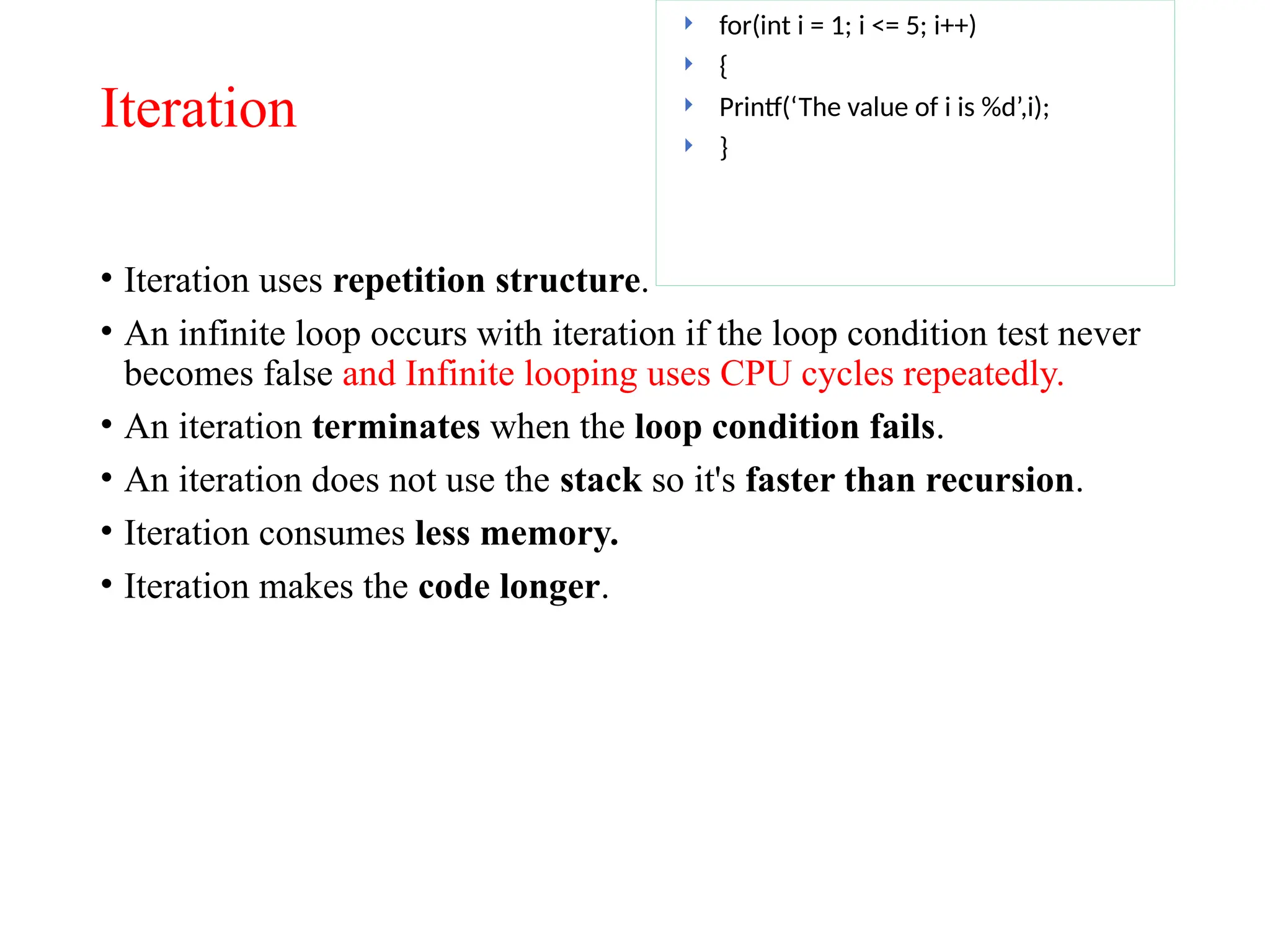
Iteration
• Iteration usesrepetition structure.
• An infinite loop occurs with iteration if the loop condition test never
becomes false and Infinite looping uses CPU cycles repeatedly.
• An iteration terminates when the loop condition fails.
• An iteration does not use the stack so it's faster than recursion.
• Iteration consumes less memory.
• Iteration makes the code longer.
for(int i = 1; i <= 5; i++)
{
Printf(‘The value of i is %d’,i);
}
UNIT 2
PART –II- SORTING
• Topics to be discussed
• SORTING
• Definition
• Different types
• Bubble sort
• Selection sort
• Insertion sort
• Merge sort
• Quick sort
• Heap sort
23.
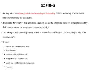
SORTING
• Sorting refersto ordering data in an increasing or decreasing fashion according to some linear
relationship among the data items.
• Telephone Directory − The telephone directory stores the telephone numbers of people sorted by
their names, so that the names can be searched easily.
• Dictionary − The dictionary stores words in an alphabetical order so that searching of any word
becomes easy.
• Types :
• Bubble sort (or) Exchange Sort.
• Selection sort.
• Insertion sort (or) Linear sort.
• Merge Sort (or) External sort.
• Quick sort (or) Partition exchange sort.
• Heap sort
24.
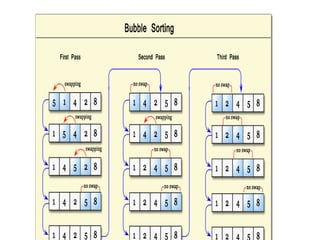
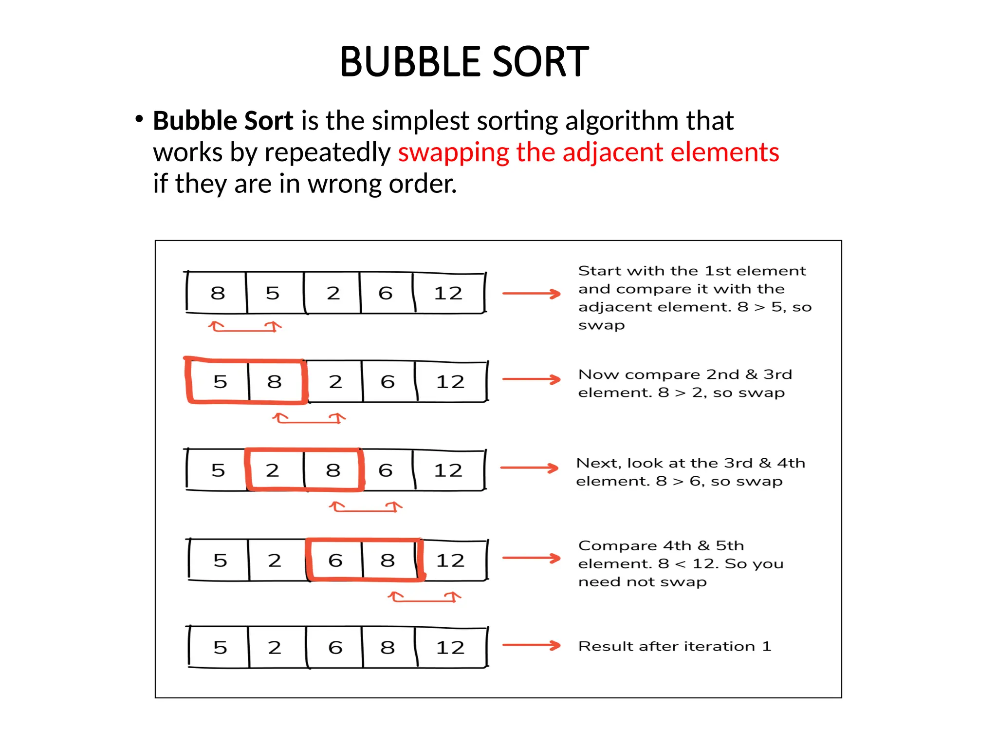
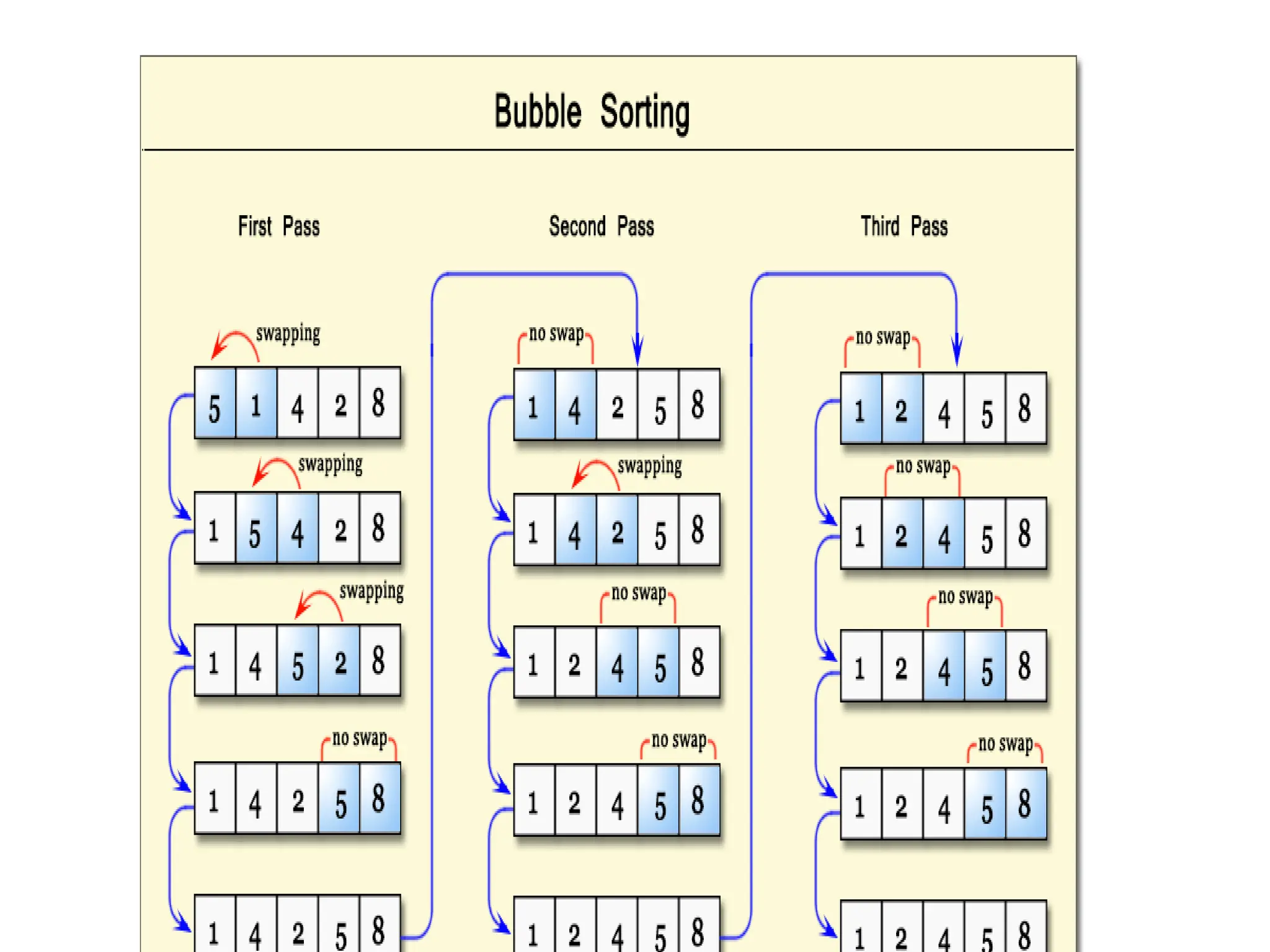
BUBBLE SORT
• BubbleSort is the simplest sorting algorithm that
works by repeatedly swapping the adjacent elements
if they are in wrong order.
26.
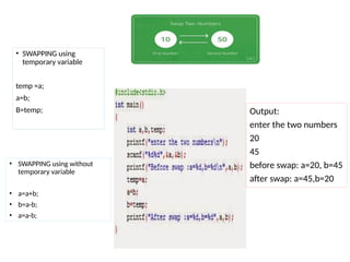
• SWAPPING using
temporaryvariable
temp =a;
a=b;
B=temp; Output:
enter the two numbers
20
45
before swap: a=20, b=45
after swap: a=45,b=20
• SWAPPING using without
temporary variable
• a=a+b;
• b=a-b;
• a=a-b;
27.
Algorithm
In the algorithmgiven below, suppose arr is an array of n elements.
The assumed swap function in the algorithm will swap the values of
given array elements.
begin BubbleSort(arr)
for all array elements
if arr[i] > arr[i+1]
swap(arr[i], arr[i+1])
end if
end for
return arr
end BubbleSort
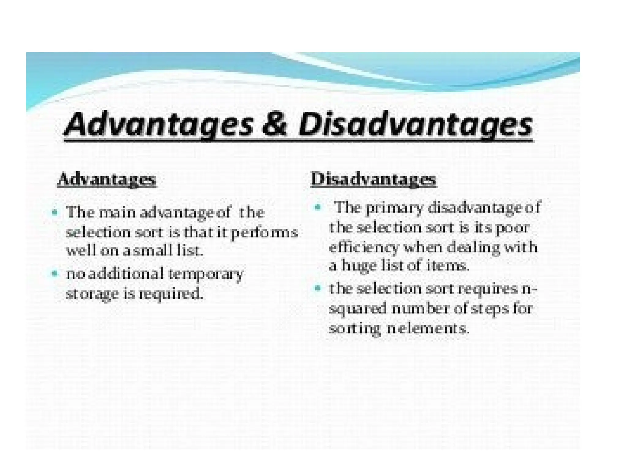
Advantage
• It's asimple algorithm that can be implemented on a computer.
• Efficient way to check if a list is already in order.
• Doesn't use too much memory.
30.
Disadvantage
• It's anefficient way to sort a list.
• Due to being efficient , the bubble sort algorithm is pretty slow for
very large lists of items.
31.
Selection sort
• Selectionsort is a simple sorting algorithm. This sorting algorithm is
comparison-based algorithm in which the list is divided into two parts, the
sorted part at the left end and the unsorted part at the right end.
• Initially, the sorted part is empty and the unsorted part is the entire list.
• The smallest element is selected from the unsorted array and swapped with the
leftmost element, and that element becomes a part of the sorted array. This
process continues moving unsorted array boundary by one element to the right.
• This algorithm is not suitable for large data sets as its best, average and worst
case complexities are of Ο(n2
), where n is the number of items.
32.
• Selection sortis a sorting algorithm that selects the smallest element
from an unsorted list in each iteration and places that element at the
beginning of the unsorted list.
33.
Working of SelectionSort
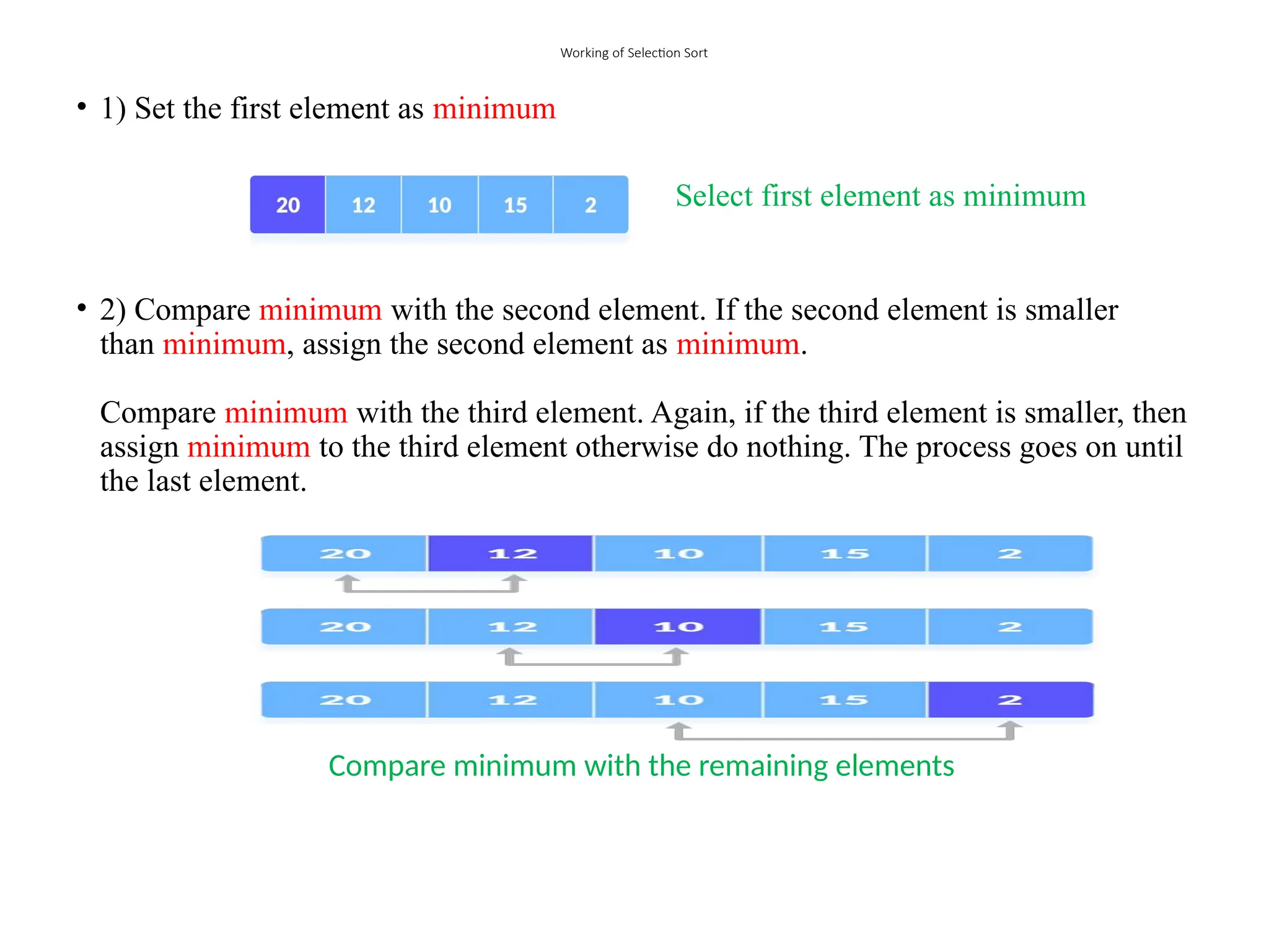
• 1) Set the first element as minimum
Select first element as minimum
• 2) Compare minimum with the second element. If the second element is smaller
than minimum, assign the second element as minimum.
Compare minimum with the third element. Again, if the third element is smaller, then
assign minimum to the third element otherwise do nothing. The process goes on until
the last element.
Compare minimum with the remaining elements
34.
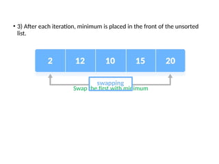
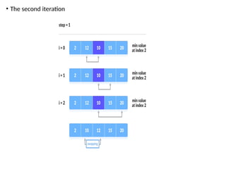
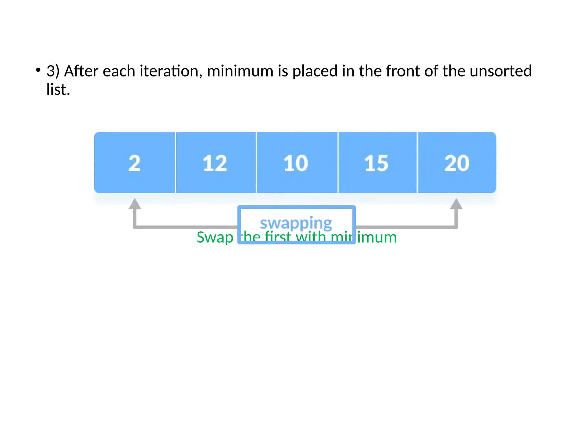
• 3) Aftereach iteration, minimum is placed in the front of the unsorted
list.
Swap the first with minimum
35.
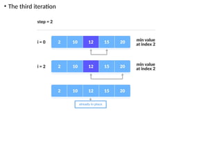
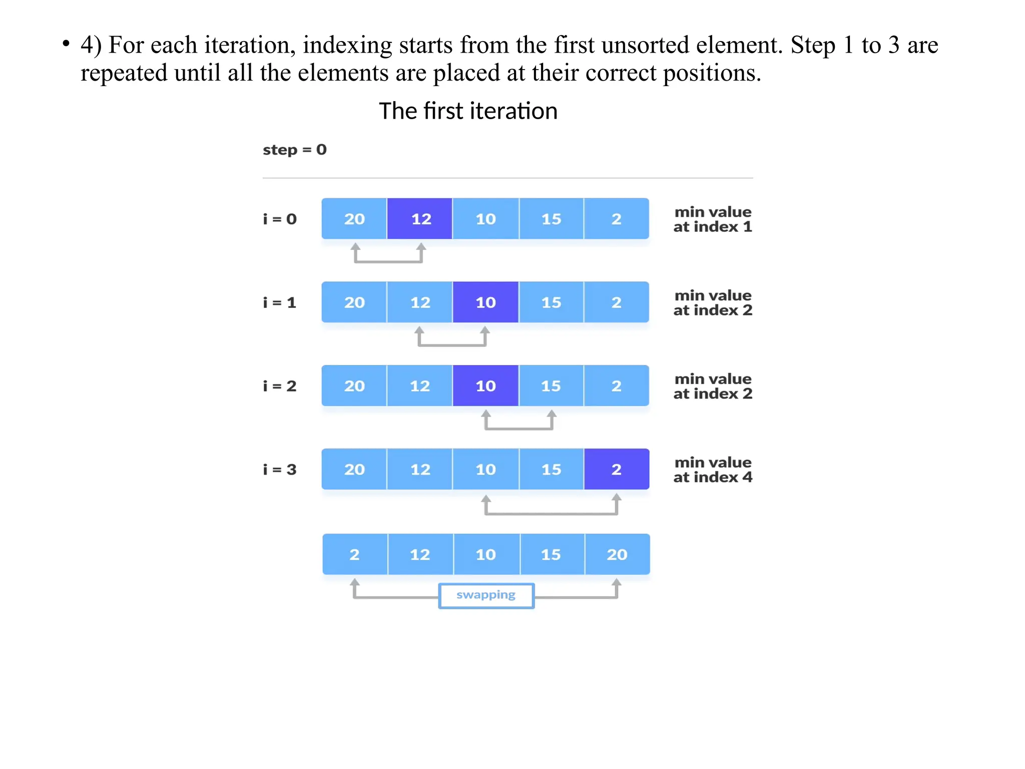
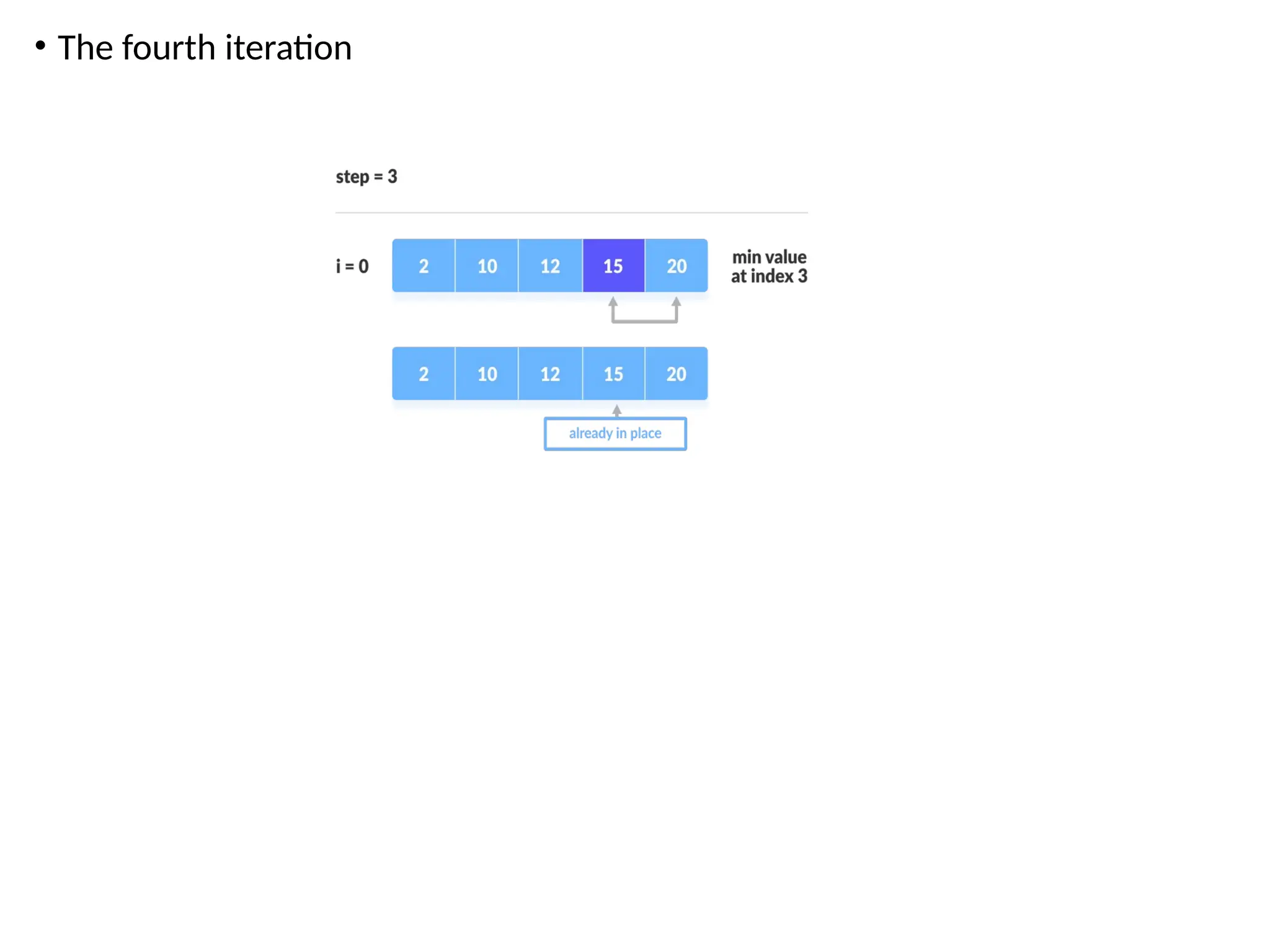
• 4) Foreach iteration, indexing starts from the first unsorted element. Step 1 to 3 are
repeated until all the elements are placed at their correct positions.
The first iteration
Complexities
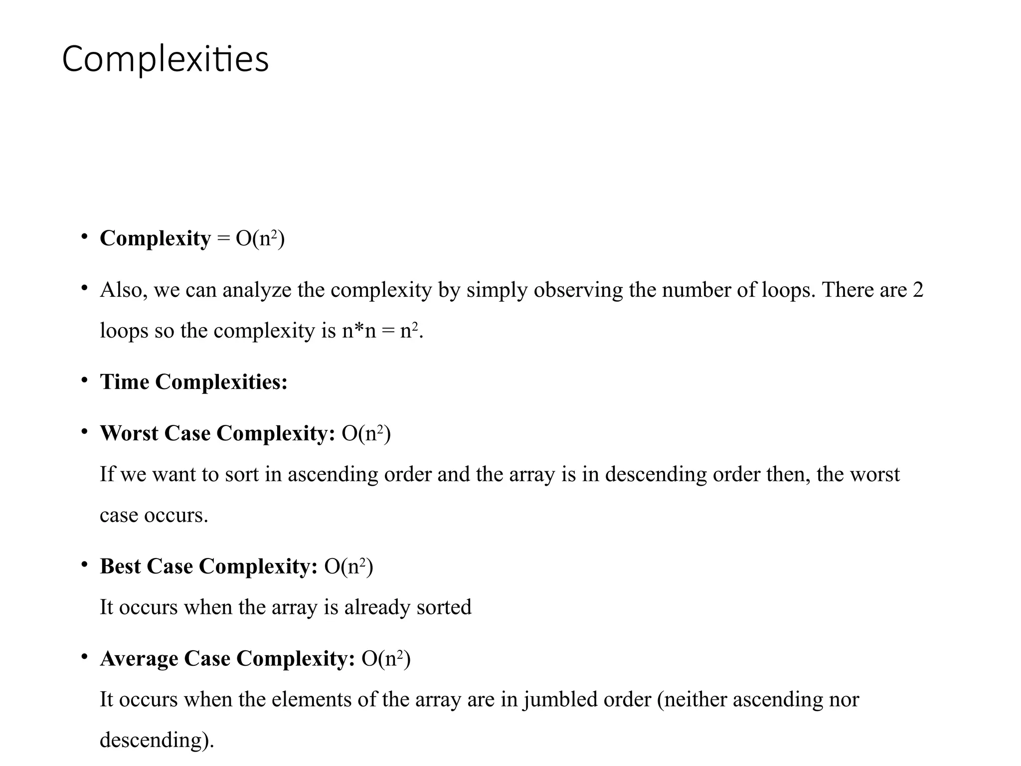
• Complexity =O(n2
)
• Also, we can analyze the complexity by simply observing the number of loops. There are 2
loops so the complexity is n*n = n2
.
• Time Complexities:
• Worst Case Complexity: O(n2
)
If we want to sort in ascending order and the array is in descending order then, the worst
case occurs.
• Best Case Complexity: O(n2
)
It occurs when the array is already sorted
• Average Case Complexity: O(n2
)
It occurs when the elements of the array are in jumbled order (neither ascending nor
descending).
42.
QUICK SORT /Partition-exchange
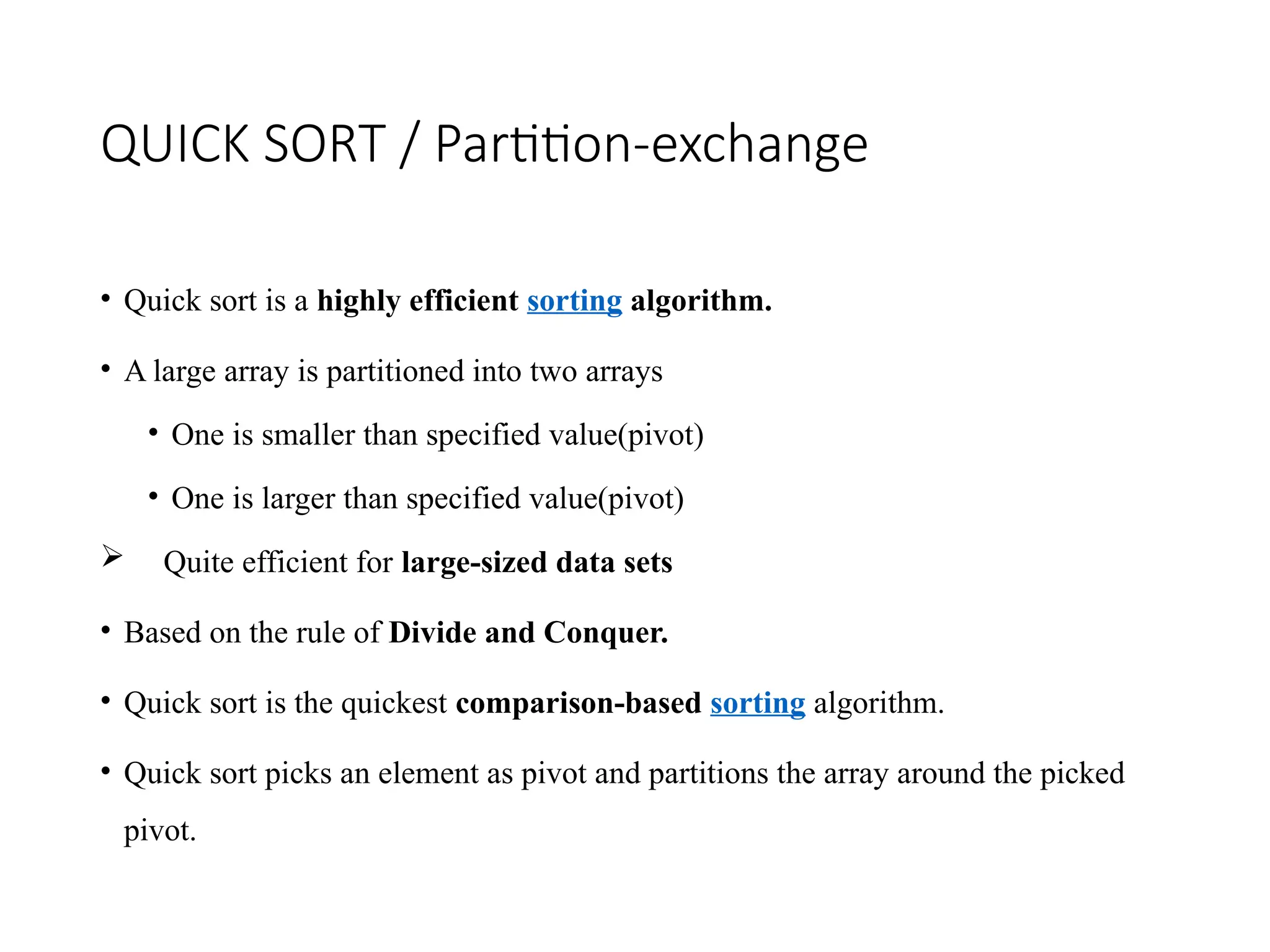
• Quick sort is a highly efficient sorting algorithm.
• A large array is partitioned into two arrays
• One is smaller than specified value(pivot)
• One is larger than specified value(pivot)
Quite efficient for large-sized data sets
• Based on the rule of Divide and Conquer.
• Quick sort is the quickest comparison-based sorting algorithm.
• Quick sort picks an element as pivot and partitions the array around the picked
pivot.
43.
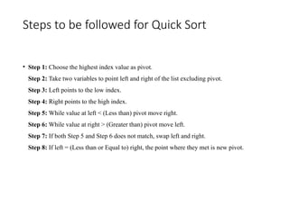
Steps to befollowed for Quick Sort
• Step 1: Choose the highest index value as pivot.
Step 2: Take two variables to point left and right of the list excluding pivot.
Step 3: Left points to the low index.
Step 4: Right points to the high index.
Step 5: While value at left < (Less than) pivot move right.
Step 6: While value at right > (Greater than) pivot move left.
Step 7: If both Step 5 and Step 6 does not match, swap left and right.
Step 8: If left = (Less than or Equal to) right, the point where they met is new pivot.
44.
EXAMPLE
• Let theelements of array are –
• In the given array, we consider the leftmost element as pivot. So, in this case, a[left] = 24,
a[right] = 27 and a[pivot] = 24.
• Since, pivot is at left, so algorithm starts from right and move towards left.
• Now, a[pivot] < a[right], so algorithm moves forward one position towards left, i.e. -
45.
• Now, a[left]= 24, a[right] = 19, and a[pivot] = 24.
• Because, a[pivot] > a[right], so, algorithm will swap a[pivot] with a[right], and pivot moves to
right, as –
• Now, a[left] = 19, a[right] = 24, and a[pivot] = 24. Since, pivot is at right, so algorithm starts
from left and moves to right.
46.
• As a[pivot]> a[left], so algorithm moves one position to right as –
• Now, a[left] = 9, a[right] = 24, and a[pivot] = 24. As a[pivot] > a[left], so algorithm moves one
position to right as -
47.
• Now, a[left]= 29, a[right] = 24, and a[pivot] = 24. As a[pivot] < a[left], so, swap a[pivot] and
a[left], now pivot is at left, i.e. –
• Since, pivot is at left, so algorithm starts from right, and move to left. Now, a[left] = 24, a[right]
= 29, and a[pivot] = 24. As a[pivot] < a[right], so algorithm moves one position to left, as -
48.
• Now, a[pivot]= 24, a[left] = 24, and a[right] = 14. As a[pivot] > a[right], so, swap a[pivot] and
a[right], now pivot is at right, i.e. –
• Now, a[pivot] = 24, a[left] = 14, and a[right] = 24. Pivot is at right, so the algorithm starts from
left and move to right.
49.
• Now, a[pivot]= 24, a[left] = 24, and a[right] = 24. So, pivot, left and right are pointing the same
element. It represents the termination of procedure.
• Element 24, which is the pivot element is placed at its exact position.
• Elements that are right side of element 24 are greater than it, and the elements that are left side
of element 24 are smaller than it.
• Now, in a similar manner, quick sort algorithm is separately applied to the left and right sub-
arrays. After sorting gets done, the array will be -
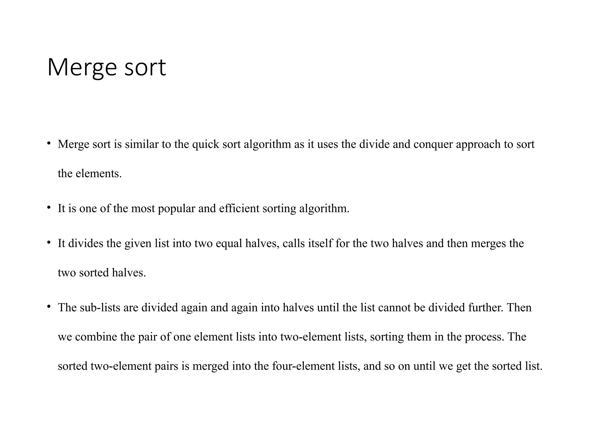
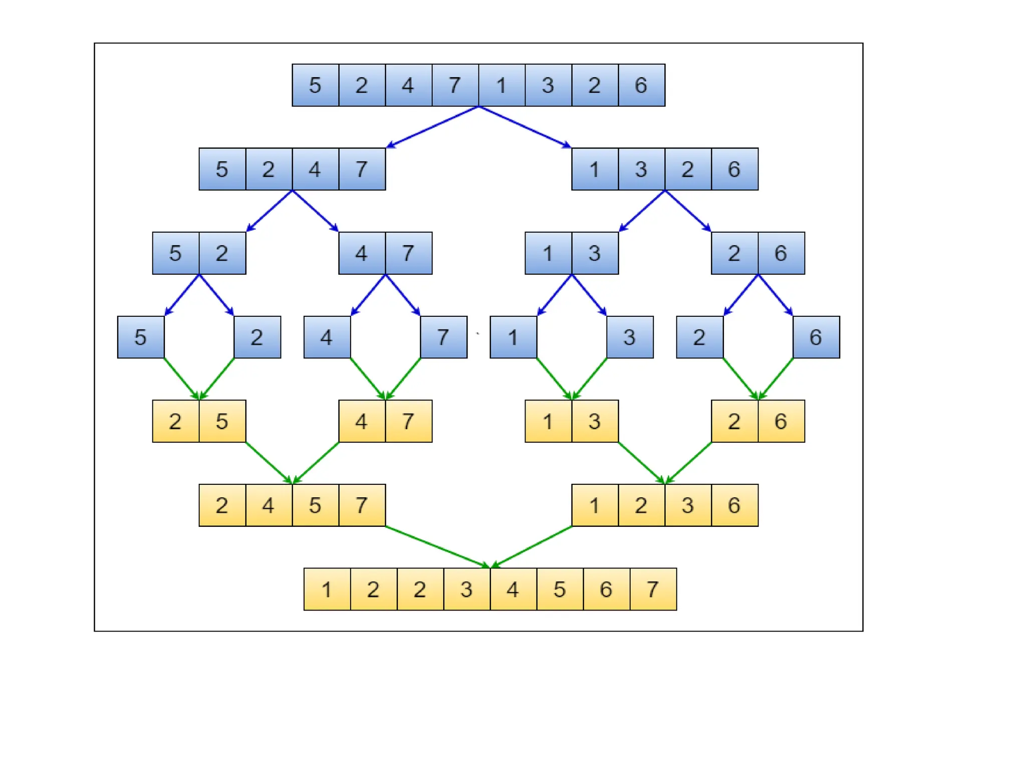
Merge sort
• Mergesort is similar to the quick sort algorithm as it uses the divide and conquer approach to sort
the elements.
• It is one of the most popular and efficient sorting algorithm.
• It divides the given list into two equal halves, calls itself for the two halves and then merges the
two sorted halves.
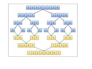
• The sub-lists are divided again and again into halves until the list cannot be divided further. Then
we combine the pair of one element lists into two-element lists, sorting them in the process. The
sorted two-element pairs is merged into the four-element lists, and so on until we get the sorted list.
54.
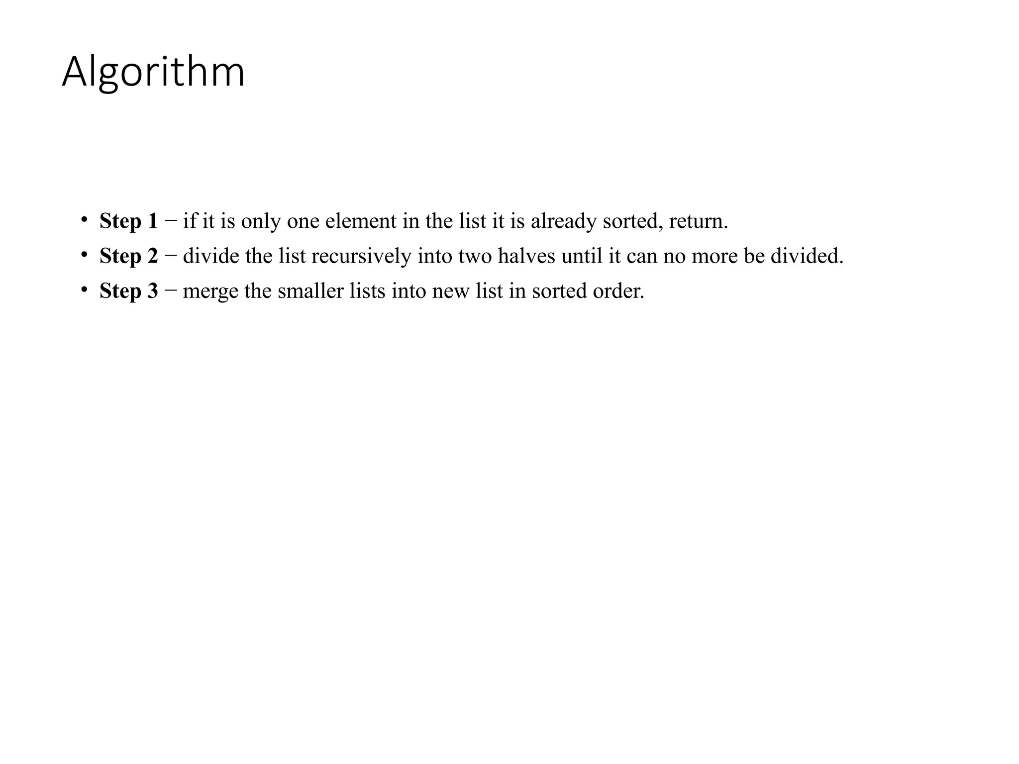
Algorithm
• Step 1− if it is only one element in the list it is already sorted, return.
• Step 2 − divide the list recursively into two halves until it can no more be divided.
• Step 3 − merge the smaller lists into new list in sorted order.
55.
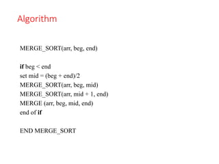
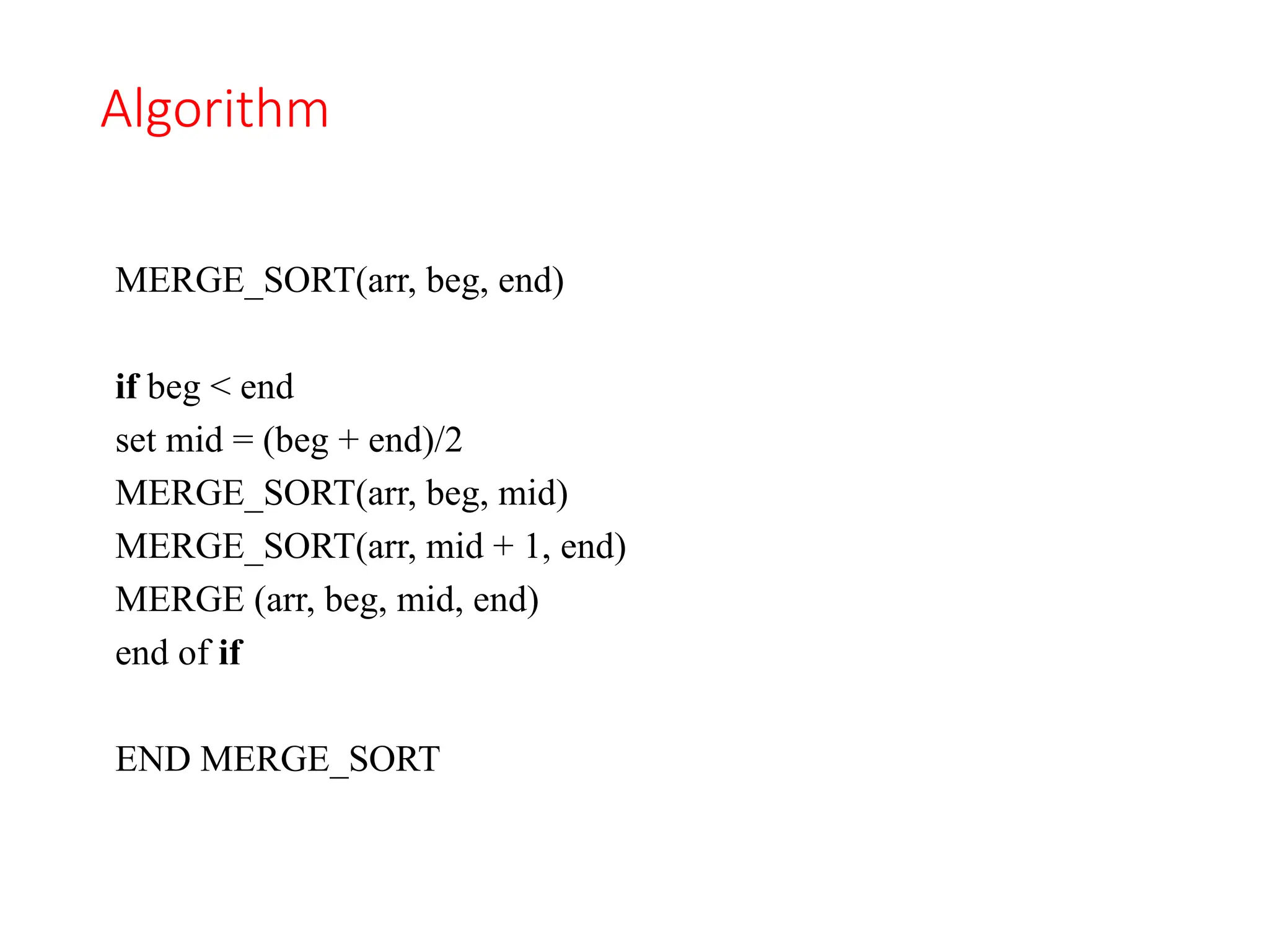
Algorithm
MERGE_SORT(arr, beg, end)
ifbeg < end
set mid = (beg + end)/2
MERGE_SORT(arr, beg, mid)
MERGE_SORT(arr, mid + 1, end)
MERGE (arr, beg, mid, end)
end of if
END MERGE_SORT
56.
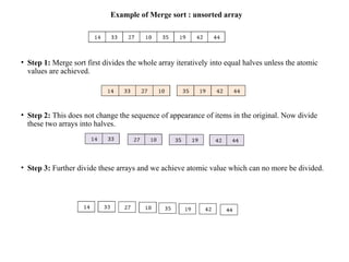
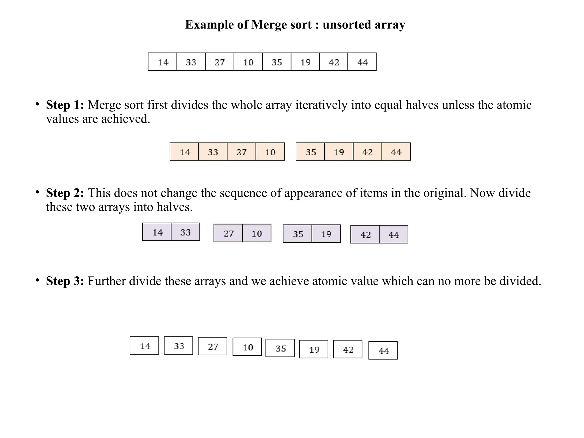
Example of Mergesort : unsorted array
• Step 1: Merge sort first divides the whole array iteratively into equal halves unless the atomic
values are achieved.
• Step 2: This does not change the sequence of appearance of items in the original. Now divide
these two arrays into halves.
• Step 3: Further divide these arrays and we achieve atomic value which can no more be divided.
57.
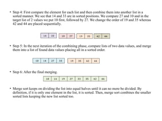
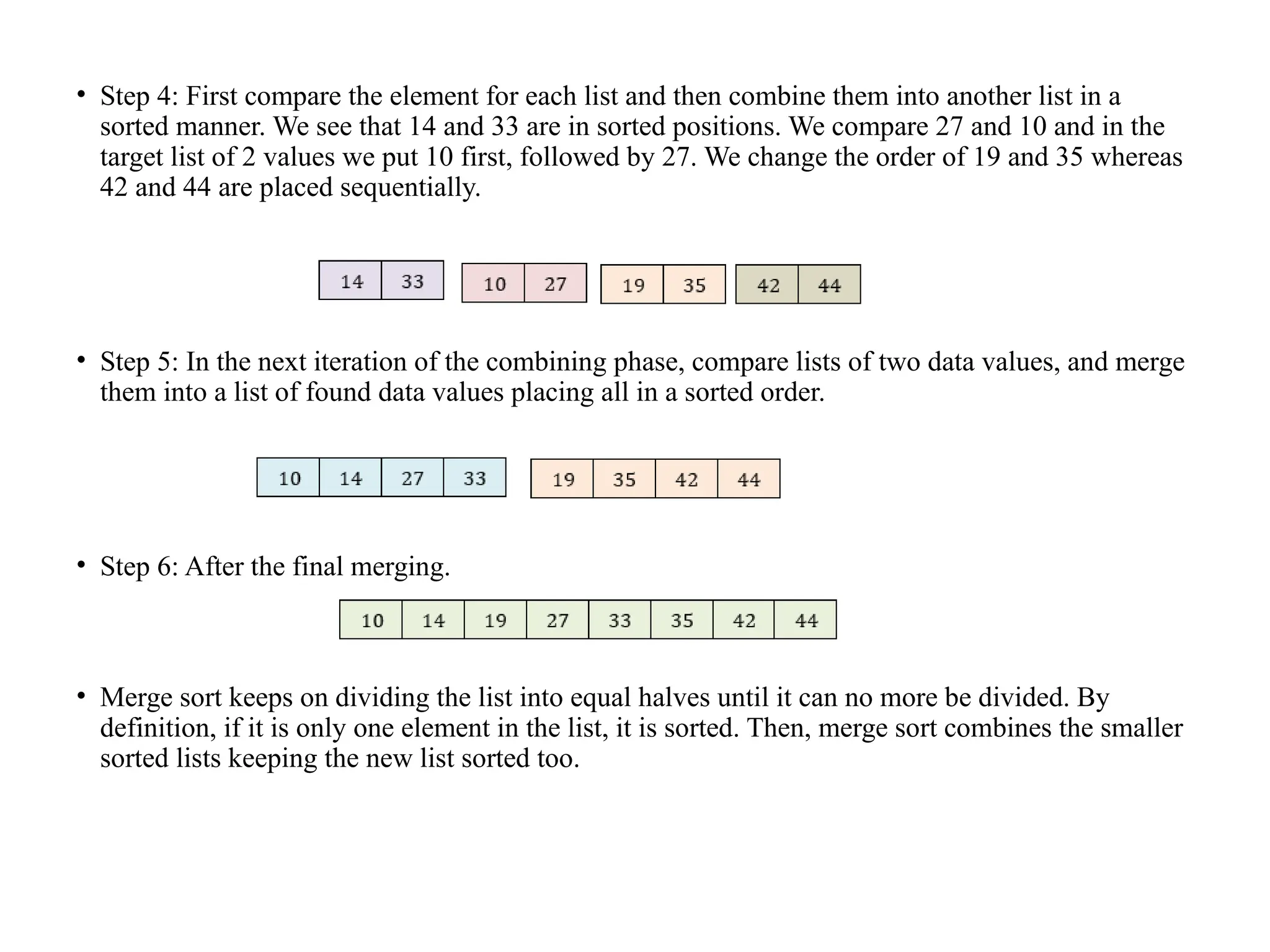
• Step 4:First compare the element for each list and then combine them into another list in a
sorted manner. We see that 14 and 33 are in sorted positions. We compare 27 and 10 and in the
target list of 2 values we put 10 first, followed by 27. We change the order of 19 and 35 whereas
42 and 44 are placed sequentially.
• Step 5: In the next iteration of the combining phase, compare lists of two data values, and merge
them into a list of found data values placing all in a sorted order.
• Step 6: After the final merging.
• Merge sort keeps on dividing the list into equal halves until it can no more be divided. By
definition, if it is only one element in the list, it is sorted. Then, merge sort combines the smaller
sorted lists keeping the new list sorted too.
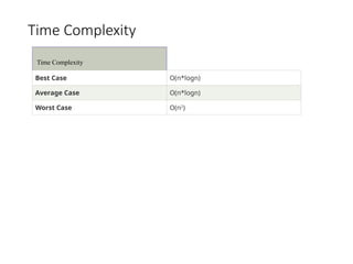
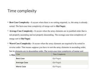
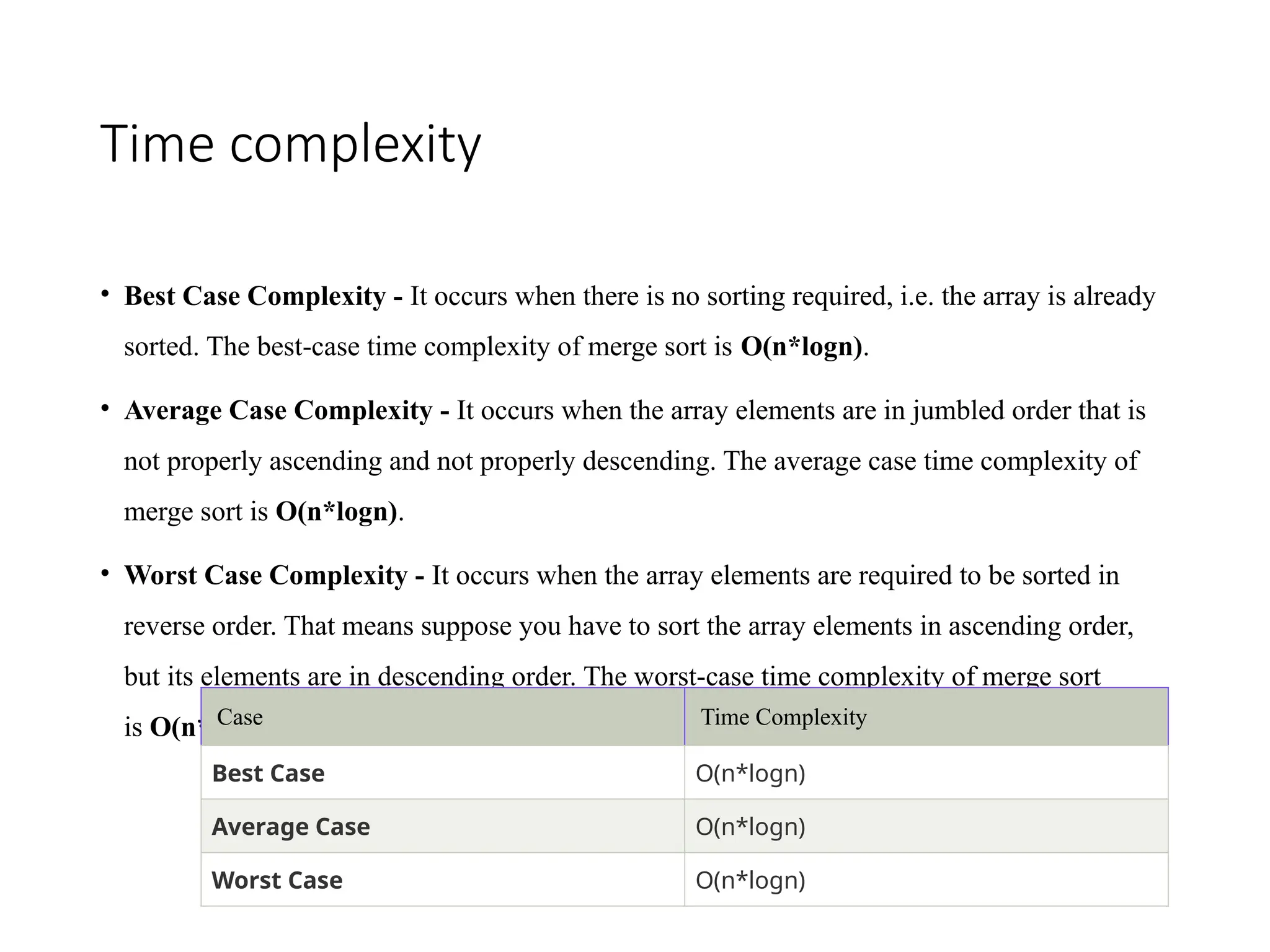
Time complexity
• BestCase Complexity - It occurs when there is no sorting required, i.e. the array is already
sorted. The best-case time complexity of merge sort is O(n*logn).
• Average Case Complexity - It occurs when the array elements are in jumbled order that is
not properly ascending and not properly descending. The average case time complexity of
merge sort is O(n*logn).
• Worst Case Complexity - It occurs when the array elements are required to be sorted in
reverse order. That means suppose you have to sort the array elements in ascending order,
but its elements are in descending order. The worst-case time complexity of merge sort
is O(n*logn).
Case Time Complexity
Best Case O(n*logn)
Average Case O(n*logn)
Worst Case O(n*logn)
61.
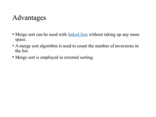
Advantages
• Merge sortcan be used with linked lists without taking up any more
space.
• A merge sort algorithm is used to count the number of inversions in
the list.
• Merge sort is employed in external sorting.
62.
Disadvantages
• For smalldatasets, merge sort is slower than other sorting algorithms.
• Even if the array is sorted, the merge sort goes through the entire
process.
63.
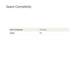
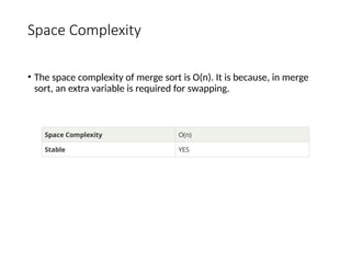
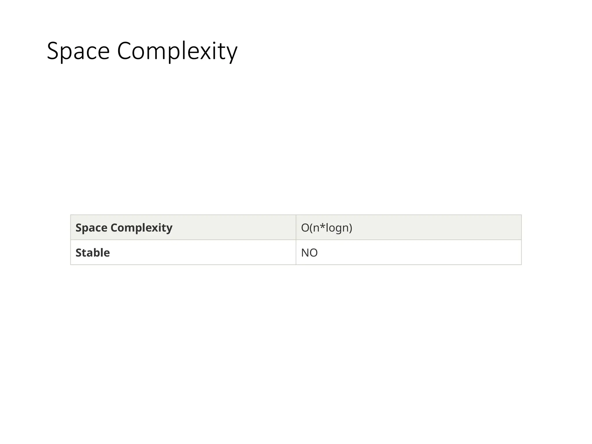
Space Complexity
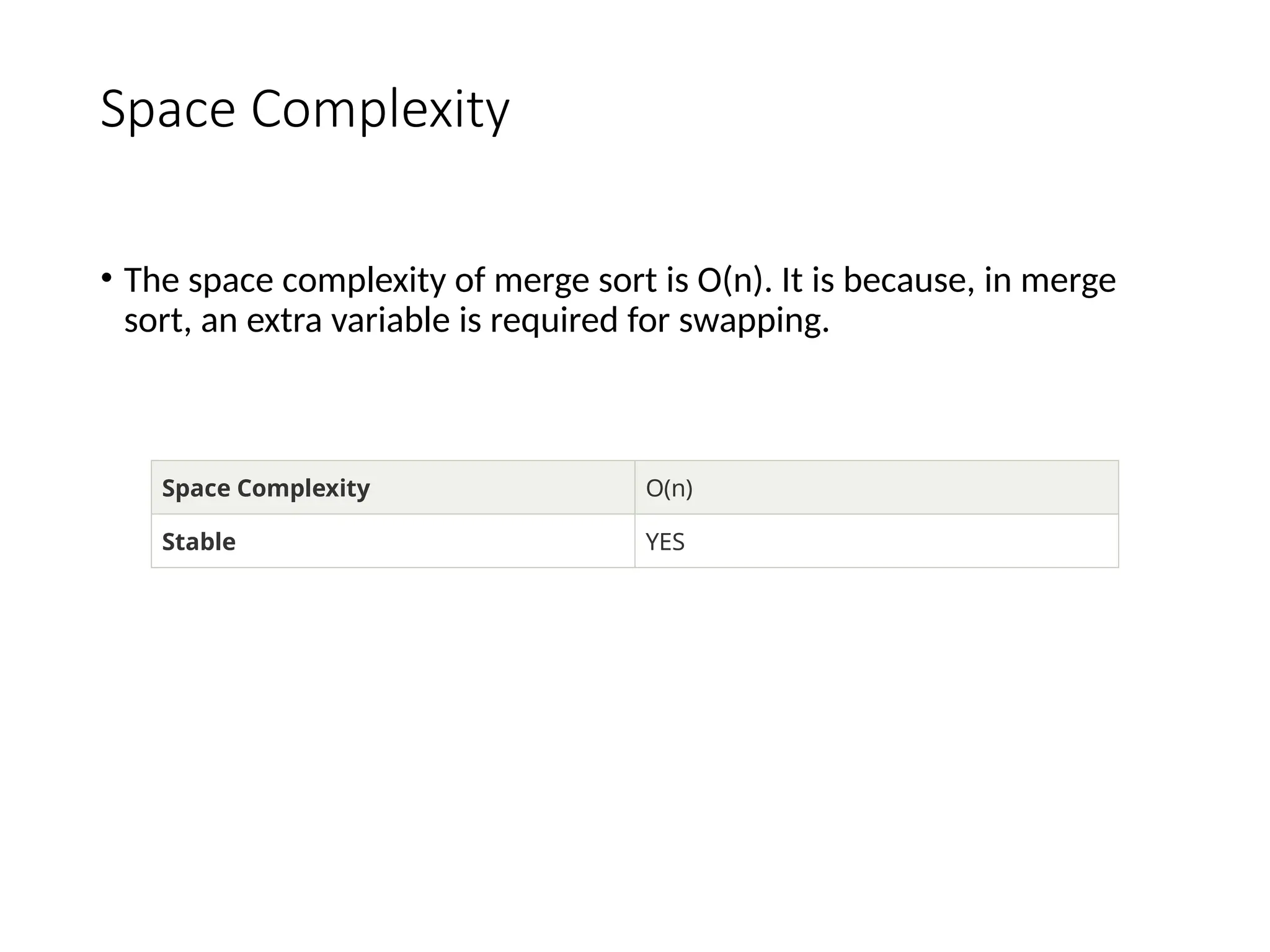
• Thespace complexity of merge sort is O(n). It is because, in merge
sort, an extra variable is required for swapping.
Space Complexity O(n)
Stable YES
64.
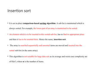
Insertion sort
• Itis an in-place comparison-based sorting algorithm. A sub-list is maintained which is
always sorted. For example, the lower part of an array is maintained to be sorted.
• An element which is to be inserted in this sorted sub-list, has to find its appropriate place
and then it has to be inserted there. Hence the name, insertion sort.
• The array is searched sequentially and unsorted items are moved and inserted into the
sorted sub-list (in the same array).
• This algorithm is not suitable for large data sets as its average and worst case complexity are
of Ο(n2
), where n is the number of items.
65.
Advantages:
• Simple implementation
•Efficient for small data sets
• Adaptive, i.e., it is appropriate for data sets that are already
substantially sorted.
66.
Algorithm
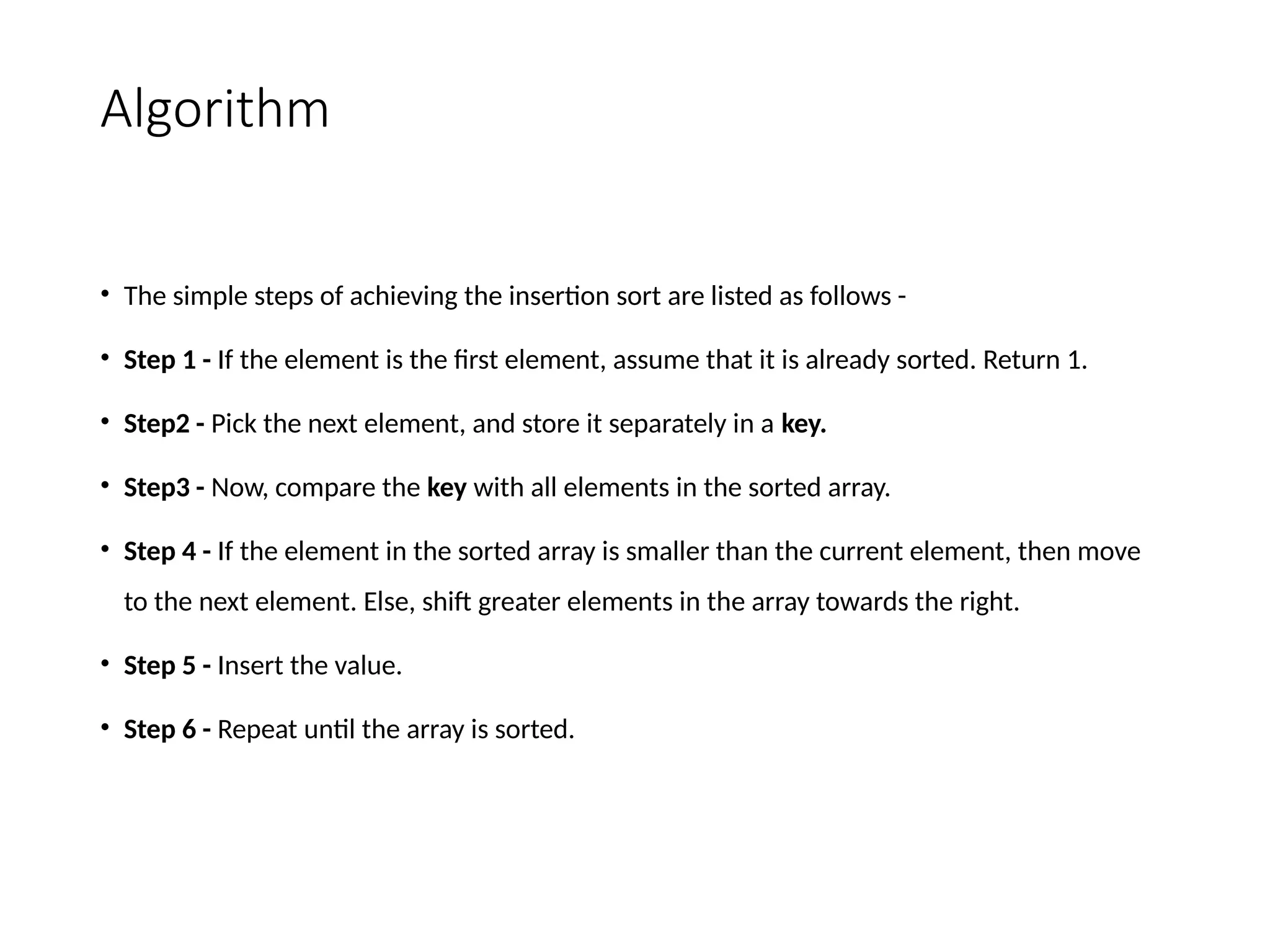
• The simplesteps of achieving the insertion sort are listed as follows -
• Step 1 - If the element is the first element, assume that it is already sorted. Return 1.
• Step2 - Pick the next element, and store it separately in a key.
• Step3 - Now, compare the key with all elements in the sorted array.
• Step 4 - If the element in the sorted array is smaller than the current element, then move
to the next element. Else, shift greater elements in the array towards the right.
• Step 5 - Insert the value.
• Step 6 - Repeat until the array is sorted.
67.
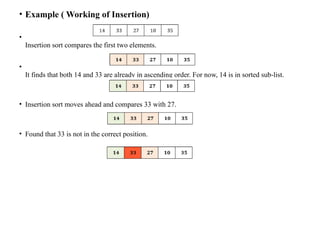
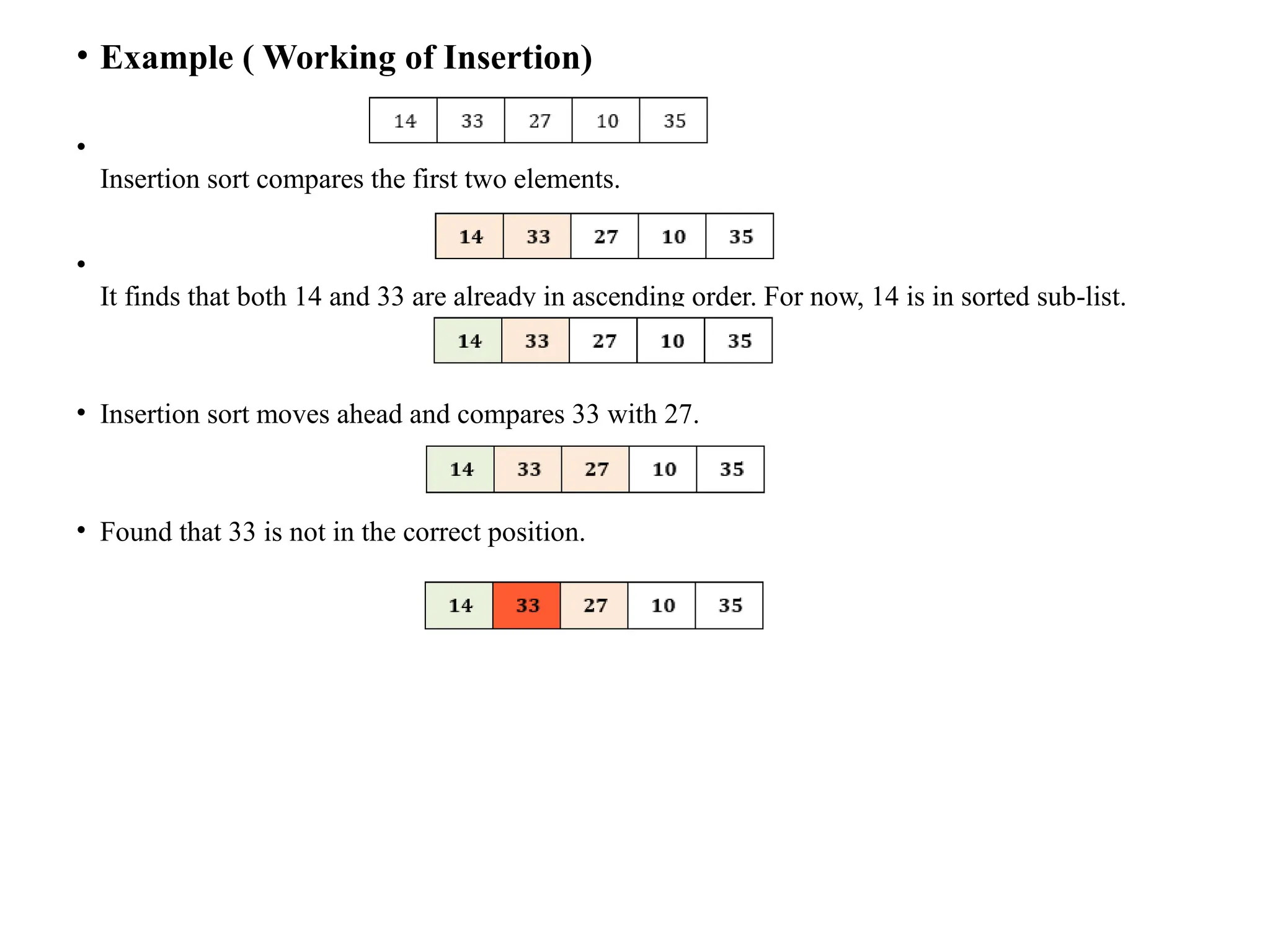
• Example (Working of Insertion)
•
Insertion sort compares the first two elements.
•
It finds that both 14 and 33 are already in ascending order. For now, 14 is in sorted sub-list.
• Insertion sort moves ahead and compares 33 with 27.
• Found that 33 is not in the correct position.
68.
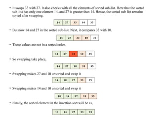
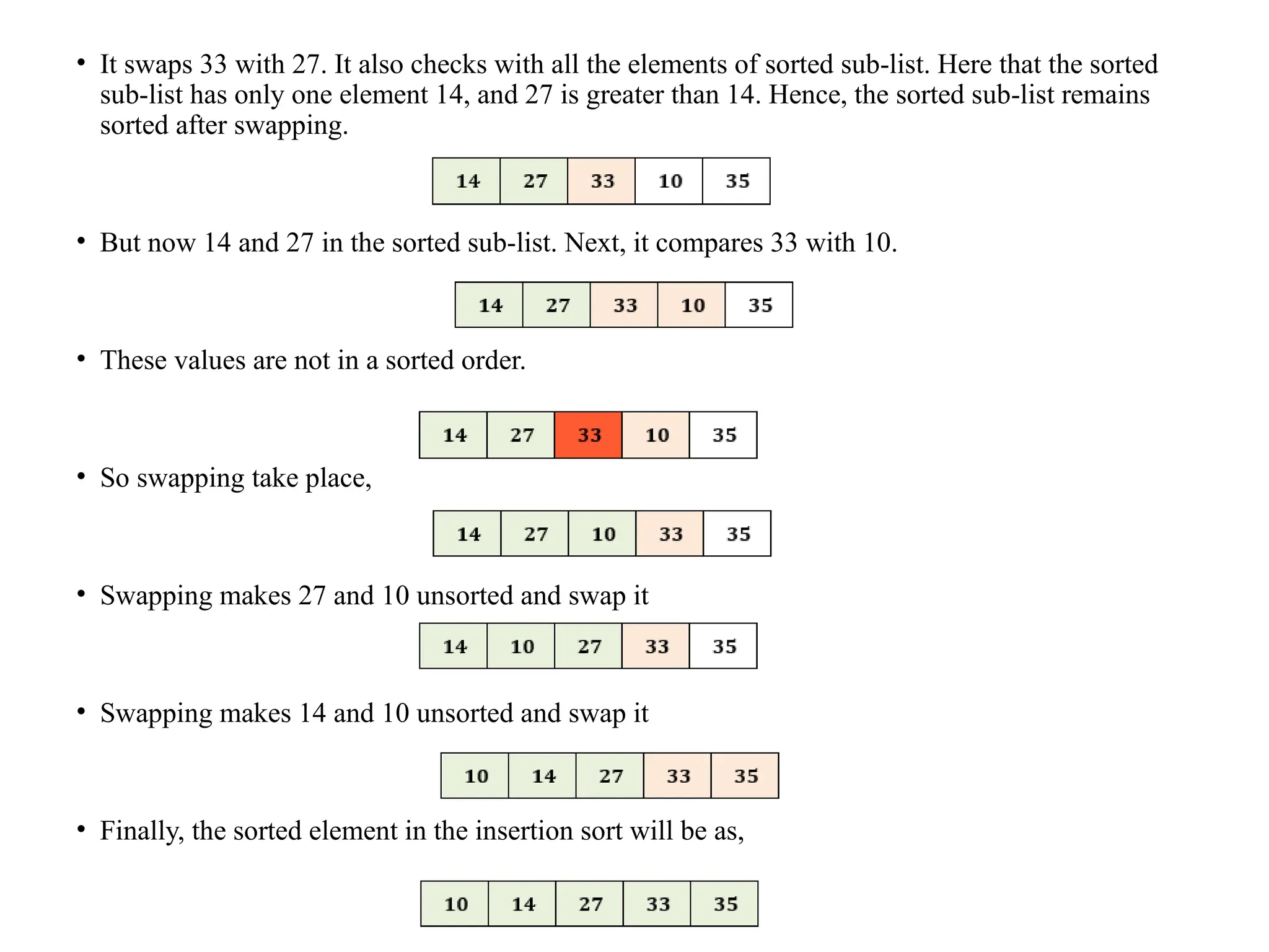
• It swaps33 with 27. It also checks with all the elements of sorted sub-list. Here that the sorted
sub-list has only one element 14, and 27 is greater than 14. Hence, the sorted sub-list remains
sorted after swapping.
• But now 14 and 27 in the sorted sub-list. Next, it compares 33 with 10.
• These values are not in a sorted order.
• So swapping take place,
• Swapping makes 27 and 10 unsorted and swap it
• Swapping makes 14 and 10 unsorted and swap it
• Finally, the sorted element in the insertion sort will be as,
69.
Implementation / program
•#include <stdio.h>
•
• void insert(int a[], int n) /
* function to sort an aay with insertion sort */
• {
• int i, j, temp;
• for (i = 1; i < n; i++) {
• temp = a[i];
• j = i - 1;
•
• while(j>=0 && temp <= a[j]) /
* Move the elements greater than temp to on
e position ahead from their current position*/
• {
• a[j+1] = a[j];
• j = j-1;
• }
• a[j+1] = temp;
• }
• }
•
void printArr(int a[], int n) /
* function to print the array */
{
int i;
for (i = 0; i < n; i++)
printf("%d ", a[i]);
}
int main()
{
int a[] = { 12, 31, 25, 8, 32, 17 };
int n = sizeof(a) / sizeof(a[0]);
printf("Before sorting array elements are - n");
printArr(a, n);
insert(a, n);
printf("nAfter sorting array elements are - n");
printArr(a, n);
return 0;
}
70.
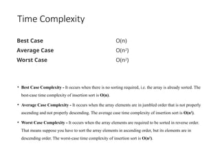
Time Complexity
• BestCase Complexity - It occurs when there is no sorting required, i.e. the array is already sorted. The
best-case time complexity of insertion sort is O(n).
• Average Case Complexity - It occurs when the array elements are in jumbled order that is not properly
ascending and not properly descending. The average case time complexity of insertion sort is O(n2
).
• Worst Case Complexity - It occurs when the array elements are required to be sorted in reverse order.
That means suppose you have to sort the array elements in ascending order, but its elements are in
descending order. The worst-case time complexity of insertion sort is O(n2
).
Best Case O(n)
Average Case O(n2
)
Worst Case O(n2
)
71.
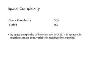
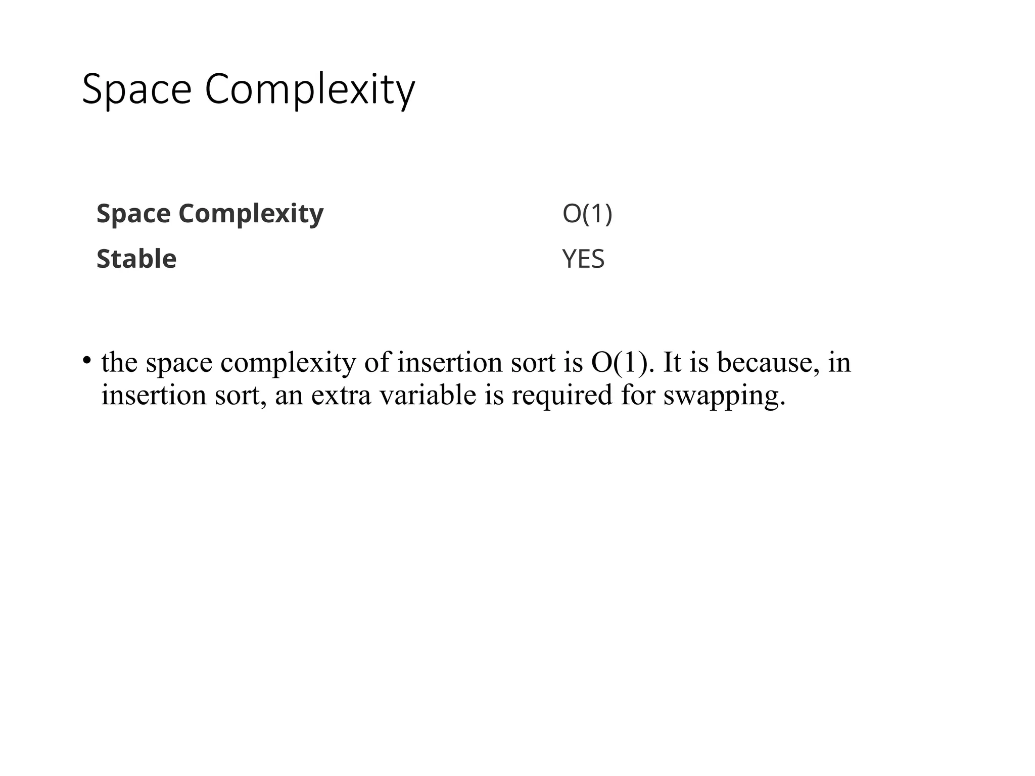
Space Complexity
• thespace complexity of insertion sort is O(1). It is because, in
insertion sort, an extra variable is required for swapping.
Space Complexity O(1)
Stable YES
Heap sort
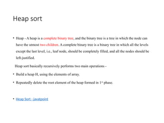
• Heap- A heap is a complete binary tree, and the binary tree is a tree in which the node can
have the utmost two children. A complete binary tree is a binary tree in which all the levels
except the last level, i.e., leaf node, should be completely filled, and all the nodes should be
left-justified.
Heap sort basically recursively performs two main operations -
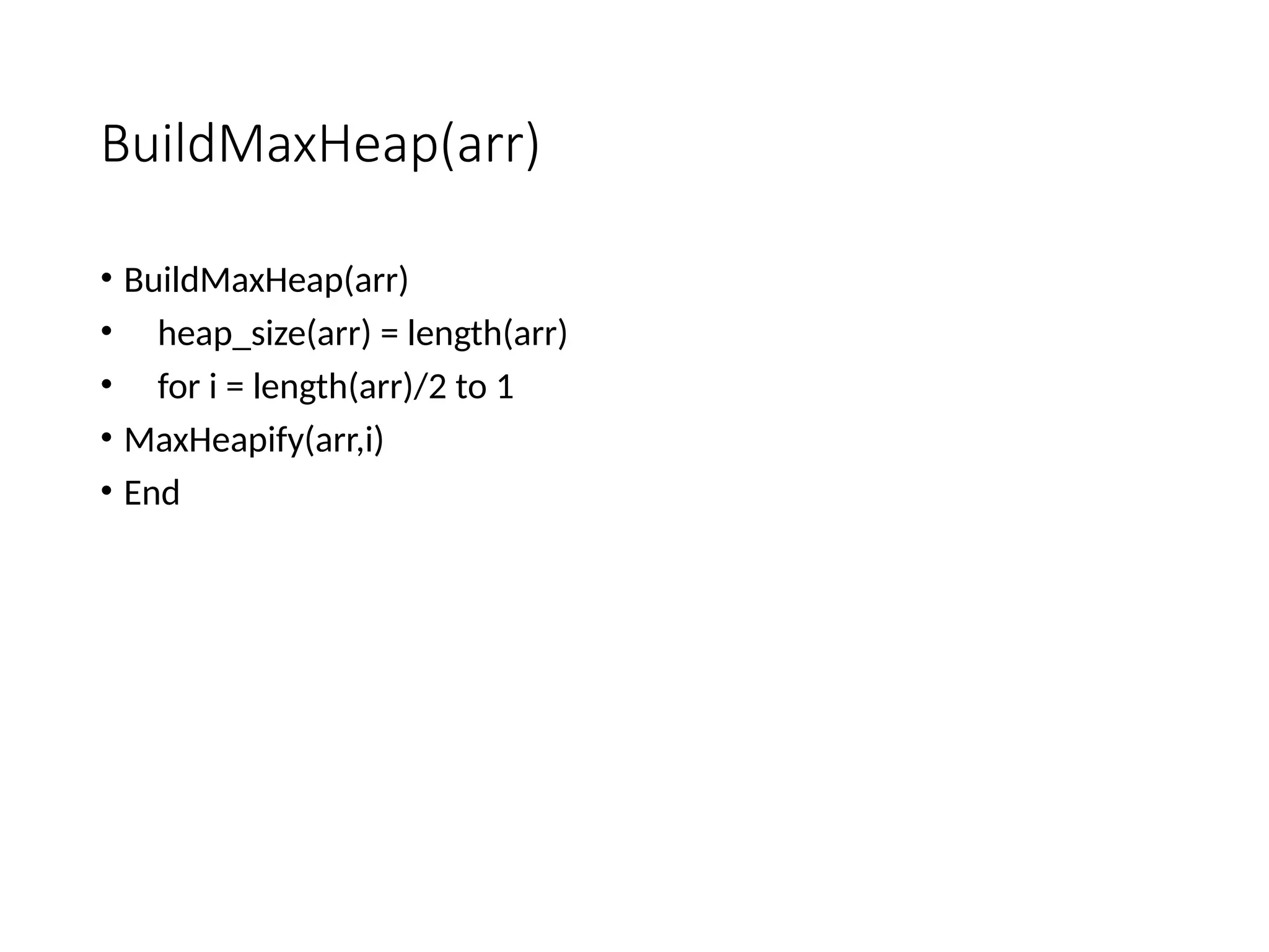
• Build a heap H, using the elements of array.
• Repeatedly delete the root element of the heap formed in 1st
phase.
• Heap Sort - javatpoint
MaxHeapify(arr,i)
• MaxHeapify(arr,i)
• L= left(i)
• R = right(i)
• if L ? heap_size[arr] and arr[L] > arr[i]
• largest = L
• else
• largest = i
• if R ? heap_size[arr] and arr[R] > arr[largest]
• largest = R
• if largest != i
• swap arr[i] with arr[largest]
• MaxHeapify(arr,largest)
• End
77.
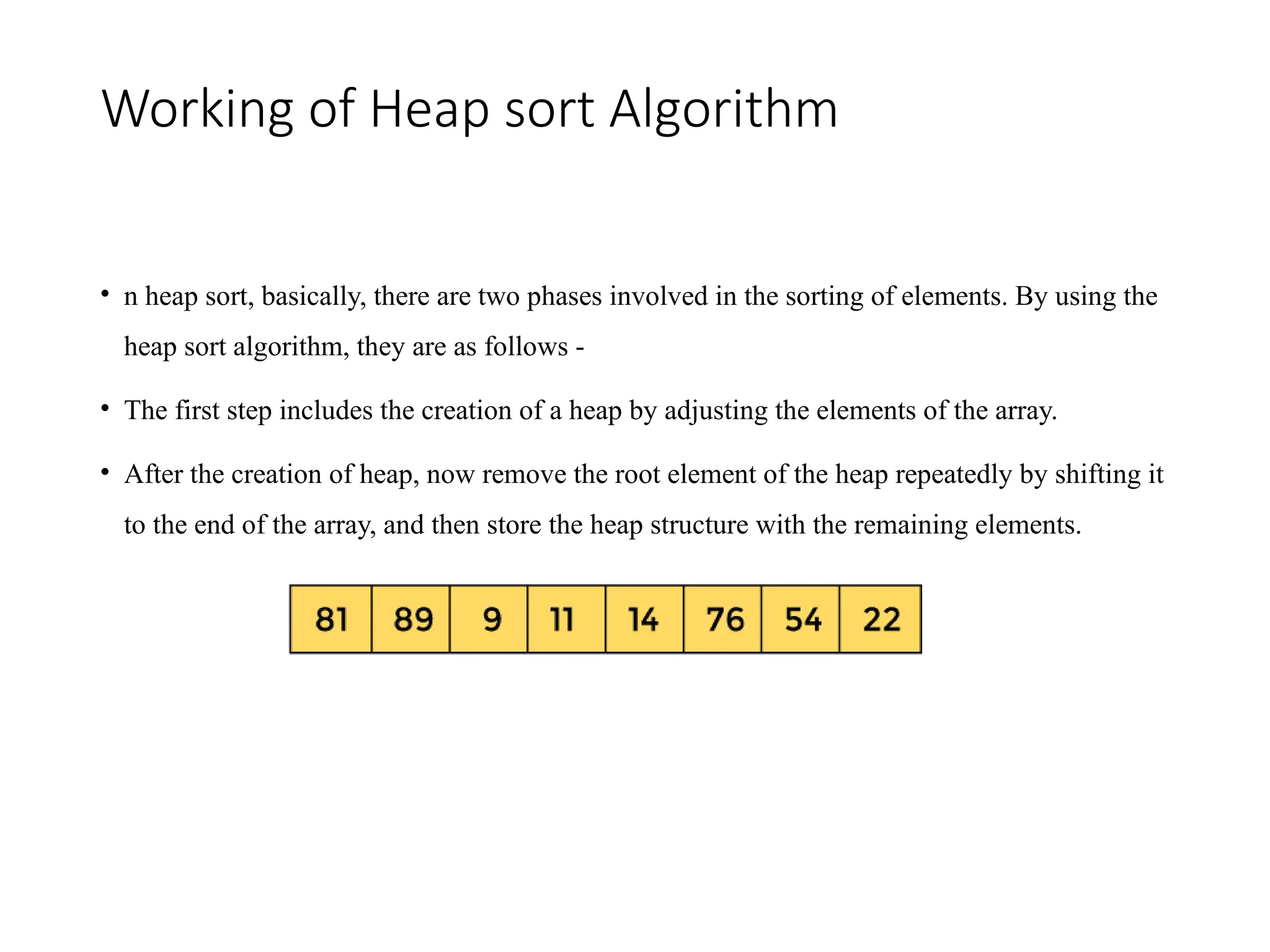
Working of Heapsort Algorithm
• n heap sort, basically, there are two phases involved in the sorting of elements. By using the
heap sort algorithm, they are as follows -
• The first step includes the creation of a heap by adjusting the elements of the array.
• After the creation of heap, now remove the root element of the heap repeatedly by shifting it
to the end of the array, and then store the heap structure with the remaining elements.
78.
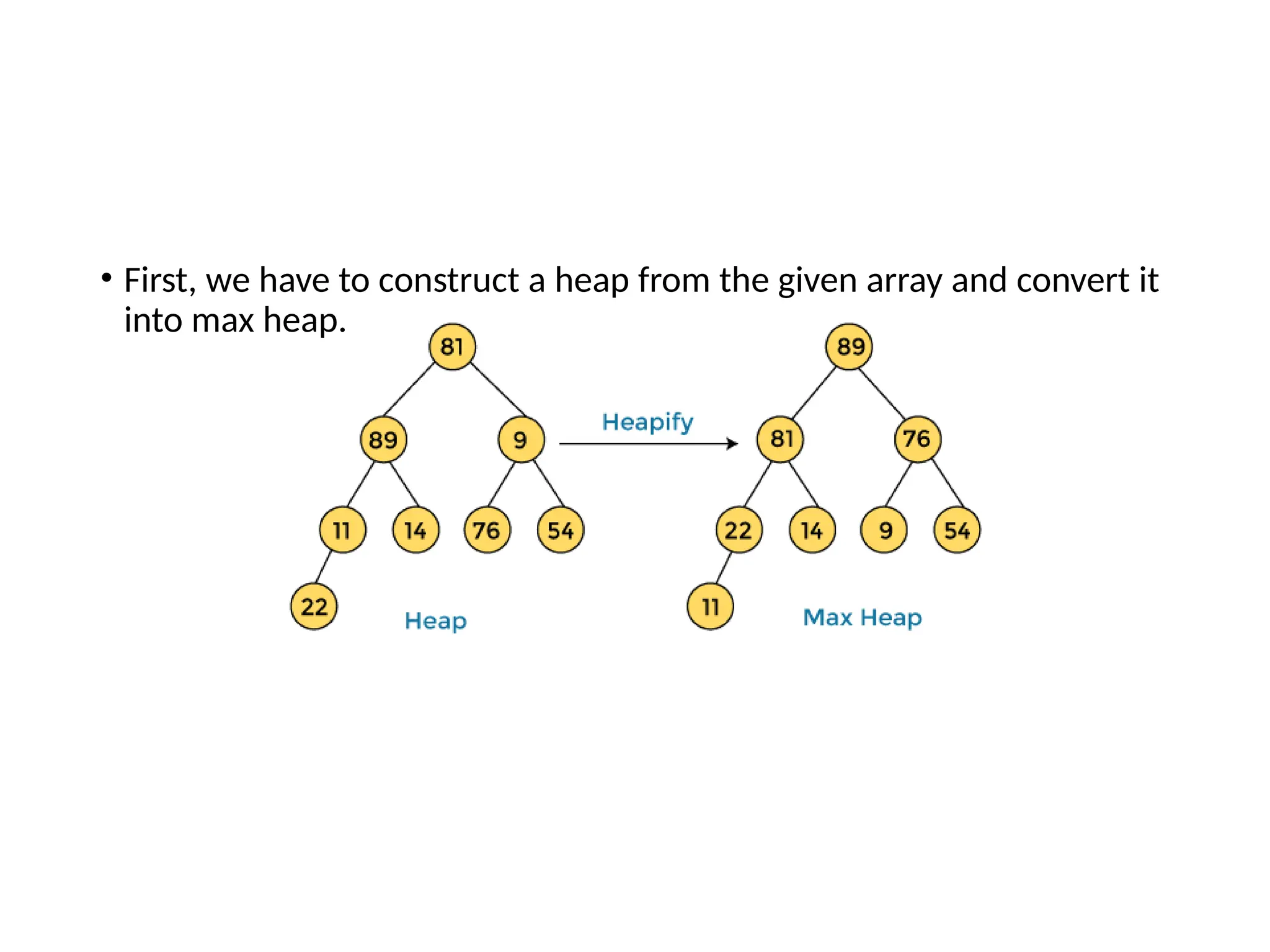
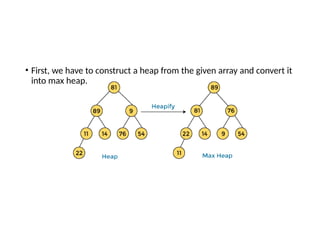
• First, wehave to construct a heap from the given array and convert it
into max heap.
79.
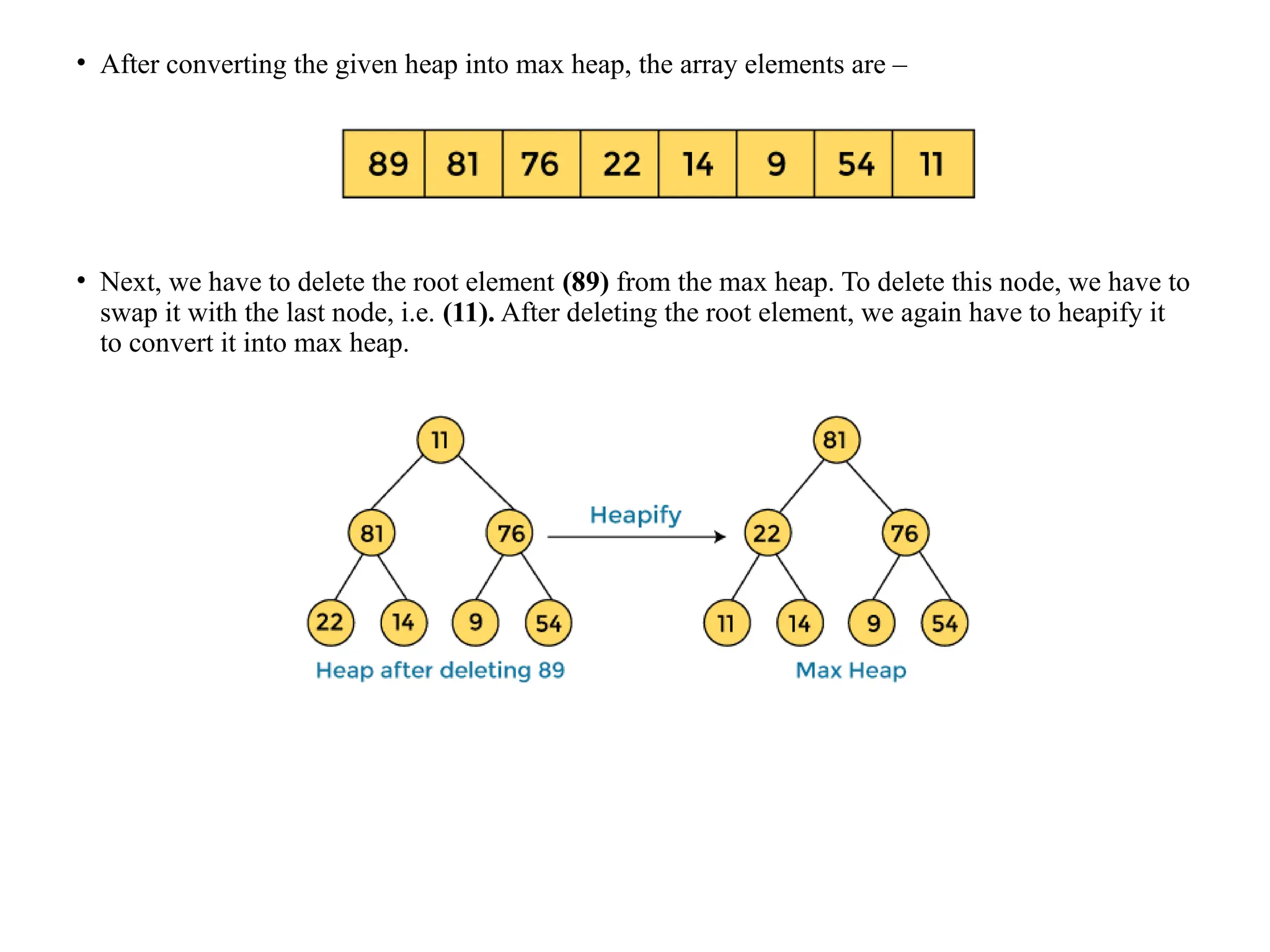
• After convertingthe given heap into max heap, the array elements are –
• Next, we have to delete the root element (89) from the max heap. To delete this node, we have to
swap it with the last node, i.e. (11). After deleting the root element, we again have to heapify it
to convert it into max heap.
80.
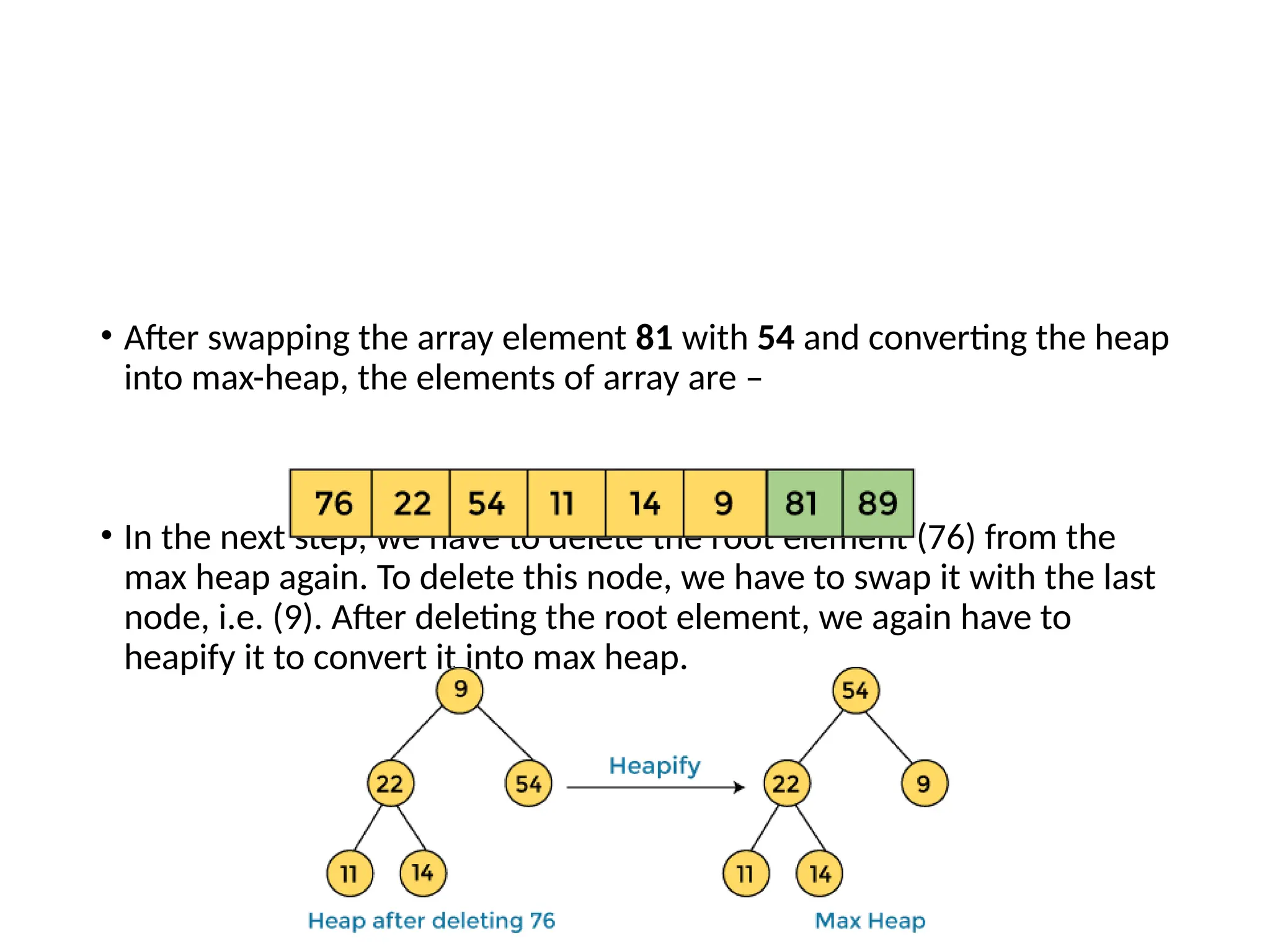
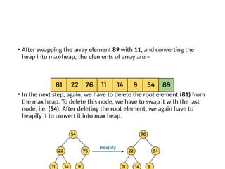
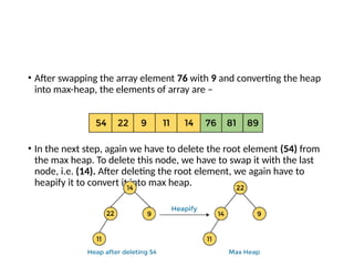
• After swappingthe array element 89 with 11, and converting the
heap into max-heap, the elements of array are –
• In the next step, again, we have to delete the root element (81) from
the max heap. To delete this node, we have to swap it with the last
node, i.e. (54). After deleting the root element, we again have to
heapify it to convert it into max heap.
81.
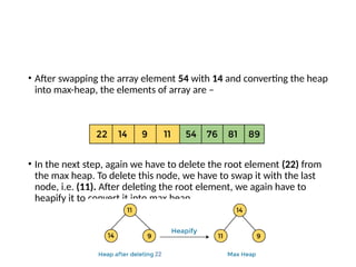
• After swappingthe array element 81 with 54 and converting the heap
into max-heap, the elements of array are –
• In the next step, we have to delete the root element (76) from the
max heap again. To delete this node, we have to swap it with the last
node, i.e. (9). After deleting the root element, we again have to
heapify it to convert it into max heap.
82.
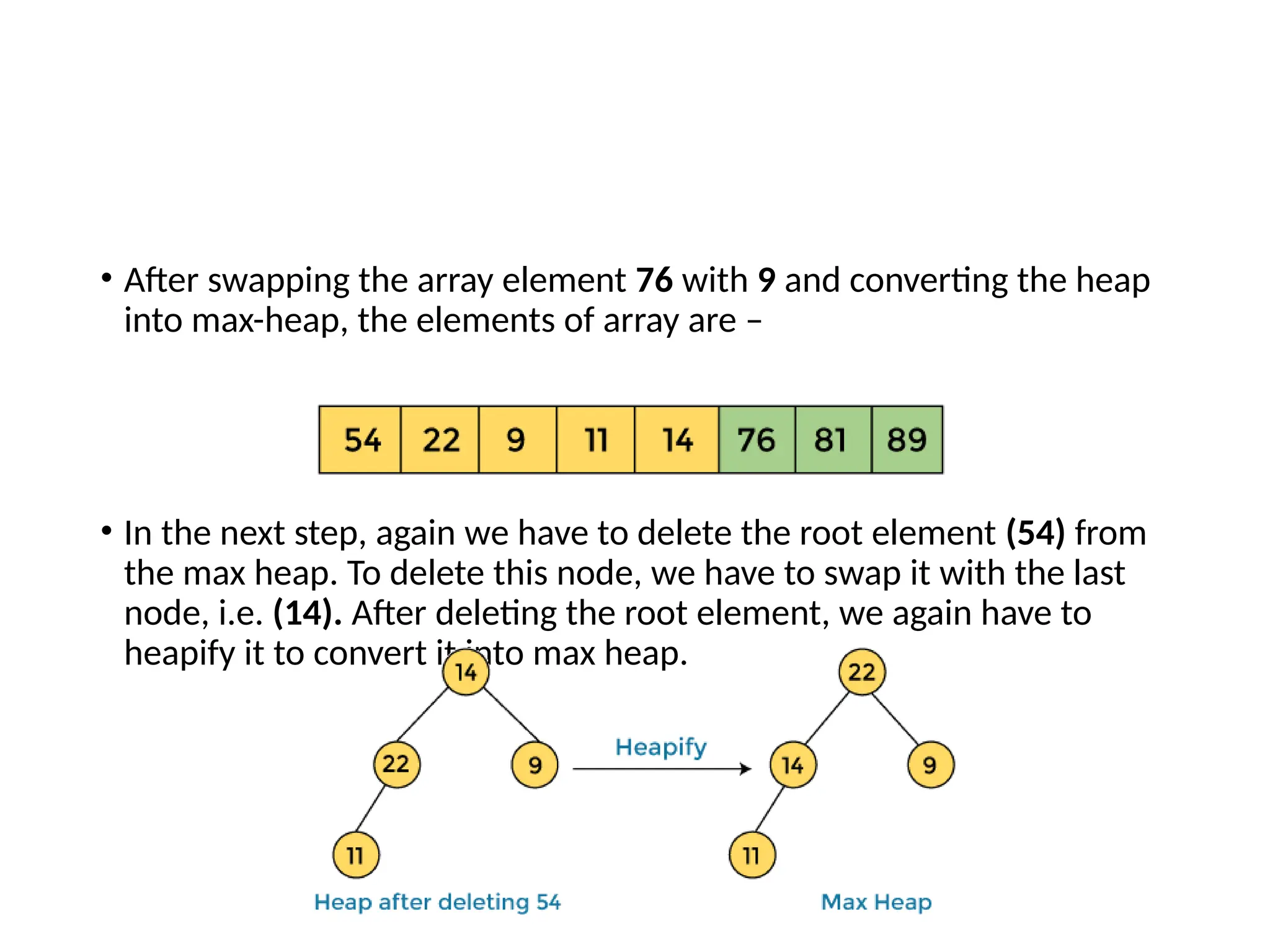
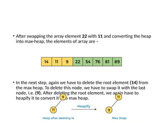
• After swappingthe array element 76 with 9 and converting the heap
into max-heap, the elements of array are –
• In the next step, again we have to delete the root element (54) from
the max heap. To delete this node, we have to swap it with the last
node, i.e. (14). After deleting the root element, we again have to
heapify it to convert it into max heap.
83.
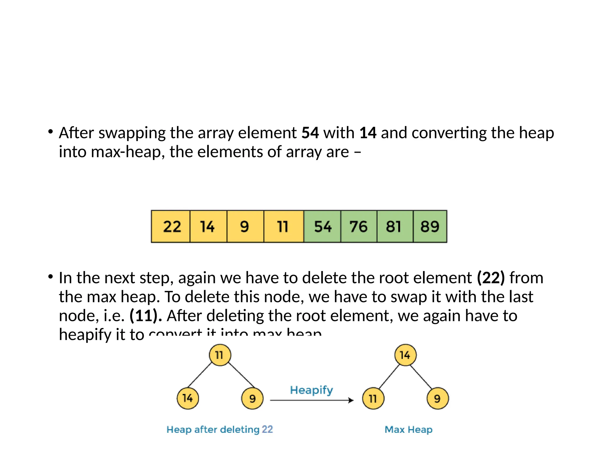
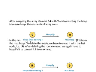
• After swappingthe array element 54 with 14 and converting the heap
into max-heap, the elements of array are –
• In the next step, again we have to delete the root element (22) from
the max heap. To delete this node, we have to swap it with the last
node, i.e. (11). After deleting the root element, we again have to
heapify it to convert it into max heap.
84.
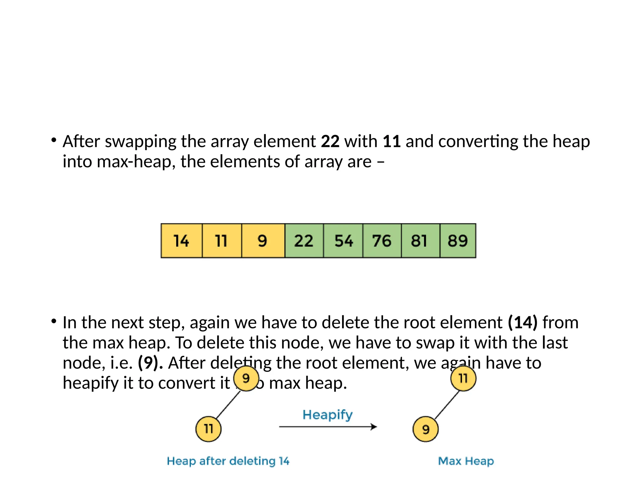
• After swappingthe array element 22 with 11 and converting the heap
into max-heap, the elements of array are –
• In the next step, again we have to delete the root element (14) from
the max heap. To delete this node, we have to swap it with the last
node, i.e. (9). After deleting the root element, we again have to
heapify it to convert it into max heap.
85.
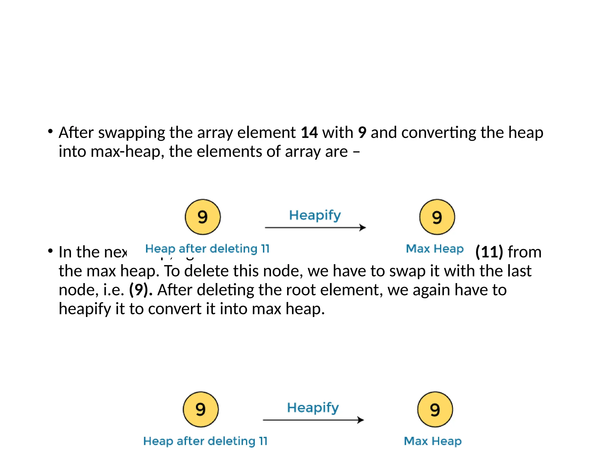
• After swappingthe array element 14 with 9 and converting the heap
into max-heap, the elements of array are –
• In the next step, again we have to delete the root element (11) from
the max heap. To delete this node, we have to swap it with the last
node, i.e. (9). After deleting the root element, we again have to
heapify it to convert it into max heap.
86.
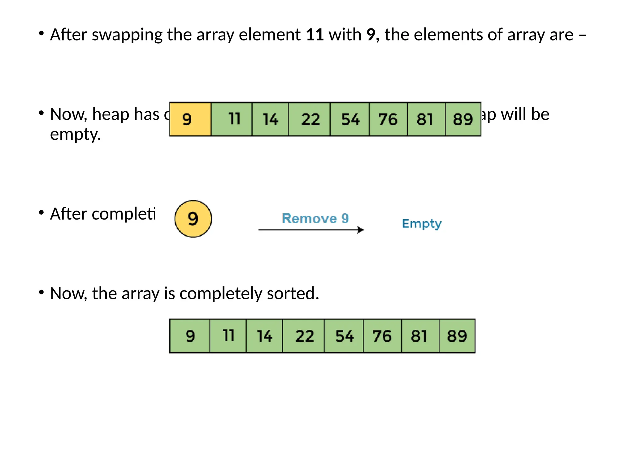
• After swappingthe array element 11 with 9, the elements of array are –
• Now, heap has only one element left. After deleting it, heap will be
empty.
• After completion of sorting, the array elements are –
• Now, the array is completely sorted.


![Algorithm: Linear Search
Algorithm: Linear Search (list [ ], n, key)
Let list [ ] be a linear array with n elements and key is an element to
be searched in the list
Step 1: Set i = 0
Step 2: while (i < n) do
If list [i] == key then
return i; //Key found at ith
location
end while
Step 3: return -1; //key not found](https://image.slidesharecdn.com/ds-unit2final-250505060355-e04c8894/85/Data-Structures-Unit-2-FINAL-presentation-pptx-8-320.jpg)
![Input: Given an array A of n elements in sorted order and item is an element to be
searched.
Output: Returns the position of item element if successful and returns -1 otherwise,
Step 1: set first = 0, last = n – 1
Step 2: while (first <= last)
mid = (first + last) / 2
if (item == A[mid])
return (mid + 1);
else if (item < A[mid])
last = mid – 1
else
first = mid + 1
end while
Step 3: return -1](https://image.slidesharecdn.com/ds-unit2final-250505060355-e04c8894/85/Data-Structures-Unit-2-FINAL-presentation-pptx-12-320.jpg)


![Algorithm
In the algorithm given below, suppose arr is an array of n elements.
The assumed swap function in the algorithm will swap the values of
given array elements.
begin BubbleSort(arr)
for all array elements
if arr[i] > arr[i+1]
swap(arr[i], arr[i+1])
end if
end for
return arr
end BubbleSort](https://image.slidesharecdn.com/ds-unit2final-250505060355-e04c8894/85/Data-Structures-Unit-2-FINAL-presentation-pptx-27-320.jpg)
![• #include<stdio.h>
• void main()
• {
• int n,i,j,temp,a[100];
• clrscr();
• printf("nEnter the size of array :");
• scanf("%d",&n);
• printf("n Enter the elementsn");
• for(i=0;i<n;i++)
• {
• scanf("%d",&a[i]);
• }
• printf("Entered array isn");
• for(i=0;i<n;i++)
• {
• printf("%dt",a[i]);
• }
•
for(i=0;i<n-1;i++)
{
for(j=0;j<n-i-1;j++)
{
if(a[j]>=a[j+1])
{
temp=a[j];
a[j]=a[j+1];
a[j+1]=temp;
}
}
}
printf("nThe sorted arrayn");
for(i=0;i<n;i++)
{
printf("%dt",a[i]);
}
getch();
}](https://image.slidesharecdn.com/ds-unit2final-250505060355-e04c8894/85/Data-Structures-Unit-2-FINAL-presentation-pptx-28-320.jpg)


![• #include<stdio.h>
• void main()
• {
• int n,i,j,small,loc,temp,a[100];
• clrscr();
• printf("nEnter the size of
array :");
• scanf("%d",&n);
• printf("n Enter the elementsn");
• for(i=0;i<n;i++)
• {
• scanf("%d",&a[i]);
• }
• printf("Entered array isn");
• for(i=0;i<n;i++)
• {
• printf("%dt",a[i]);
• }
•
for(i=0;i<=n;i++)
{ small=a[i];
loc=i;
for(j=i+1;j<n;j++)
{
if(a[j]<small)
{
small=a[j];
loc=j;
}
}
a[loc]=a[i];
a[i]=small;
}
printf("nThe sorted array isn");
for(i=0;i<n;i++)
{
printf("%dt",a[i]);
}
getch();
}](https://image.slidesharecdn.com/ds-unit2final-250505060355-e04c8894/85/Data-Structures-Unit-2-FINAL-presentation-pptx-39-320.jpg)


![EXAMPLE
• Let the elements of array are –
• In the given array, we consider the leftmost element as pivot. So, in this case, a[left] = 24,
a[right] = 27 and a[pivot] = 24.
• Since, pivot is at left, so algorithm starts from right and move towards left.
• Now, a[pivot] < a[right], so algorithm moves forward one position towards left, i.e. -](https://image.slidesharecdn.com/ds-unit2final-250505060355-e04c8894/85/Data-Structures-Unit-2-FINAL-presentation-pptx-44-320.jpg)
![• Now, a[left] = 24, a[right] = 19, and a[pivot] = 24.
• Because, a[pivot] > a[right], so, algorithm will swap a[pivot] with a[right], and pivot moves to
right, as –
• Now, a[left] = 19, a[right] = 24, and a[pivot] = 24. Since, pivot is at right, so algorithm starts
from left and moves to right.](https://image.slidesharecdn.com/ds-unit2final-250505060355-e04c8894/85/Data-Structures-Unit-2-FINAL-presentation-pptx-45-320.jpg)
![• As a[pivot] > a[left], so algorithm moves one position to right as –
• Now, a[left] = 9, a[right] = 24, and a[pivot] = 24. As a[pivot] > a[left], so algorithm moves one
position to right as -](https://image.slidesharecdn.com/ds-unit2final-250505060355-e04c8894/85/Data-Structures-Unit-2-FINAL-presentation-pptx-46-320.jpg)
![• Now, a[left] = 29, a[right] = 24, and a[pivot] = 24. As a[pivot] < a[left], so, swap a[pivot] and
a[left], now pivot is at left, i.e. –
• Since, pivot is at left, so algorithm starts from right, and move to left. Now, a[left] = 24, a[right]
= 29, and a[pivot] = 24. As a[pivot] < a[right], so algorithm moves one position to left, as -](https://image.slidesharecdn.com/ds-unit2final-250505060355-e04c8894/85/Data-Structures-Unit-2-FINAL-presentation-pptx-47-320.jpg)
![• Now, a[pivot] = 24, a[left] = 24, and a[right] = 14. As a[pivot] > a[right], so, swap a[pivot] and
a[right], now pivot is at right, i.e. –
• Now, a[pivot] = 24, a[left] = 14, and a[right] = 24. Pivot is at right, so the algorithm starts from
left and move to right.](https://image.slidesharecdn.com/ds-unit2final-250505060355-e04c8894/85/Data-Structures-Unit-2-FINAL-presentation-pptx-48-320.jpg)
![• Now, a[pivot] = 24, a[left] = 24, and a[right] = 24. So, pivot, left and right are pointing the same
element. It represents the termination of procedure.
• Element 24, which is the pivot element is placed at its exact position.
• Elements that are right side of element 24 are greater than it, and the elements that are left side
of element 24 are smaller than it.
• Now, in a similar manner, quick sort algorithm is separately applied to the left and right sub-
arrays. After sorting gets done, the array will be -](https://image.slidesharecdn.com/ds-unit2final-250505060355-e04c8894/85/Data-Structures-Unit-2-FINAL-presentation-pptx-49-320.jpg)
![• QUICK SORT
• #include<stdio.h>
• void main()
• {
• int i,n,a[50];
• void quicksort(int a[],int,int);
• clrscr();
• printf("nEnter the size of the array : ");
• scanf("%d",&n);
• printf("Enter the elements of the arraynt");
• for(i=0;i<n;i++)
• {
• scanf("%d",&a[i]);
• }
• printf("nThe entered unsorted arrayn");
• for(i=0;i<n;i++)
• {
• printf("t%d",a[i]);
• }
• quicksort(a,0,n-1);
• printf("nSorted Arrayn");
• for(i=0;i<n;i++)
• {
• printf("t%d",a[i]);
• }
• getch();
• }
void quicksort(int a[],int low,int high)
{
int pivot,down,up,key,temp;
if(low<high)
{
down=low;
pivot=low;
up=high;
key=a[pivot];
while(down<up)
{
while((a[down]<=key)&&(down<=high))
down++;
while((a[up]>key)&&(up>=low))
up--;
if(down<up)
{
temp=a[up];
a[up]=a[down];
a[down]=temp;
}
}
temp=a[up];
a[up]=a[pivot];
a[pivot]=temp;
quicksort(a,low,up-1);
quicksort(a,up+1,high);
}](https://image.slidesharecdn.com/ds-unit2final-250505060355-e04c8894/85/Data-Structures-Unit-2-FINAL-presentation-pptx-50-320.jpg)
![• #include<stdio.h>
• #include<conio.h>
• void partition(int [20],int,int);
• void merge(int [20],int,int,int);
• void main()
• {
• int i,a[20],n;
• clrscr();
• printf("Enter the number of elementsn");
• scanf("%d",&n);
• printf("Enter the elementsn");
• for(i=0;i<n;i++)
• scanf("%d",&a[i]);
• printf("Orginal listn");
• for(i=0;i<n;i++)
• printf("%dt",a[i]);
• partition(a,0,n-1);
• printf("nSorted listn");
• for(i=0;i<n;i++)
• printf("%dt",a[i]);
• getch();
• }
• void partition(int a[20],int lb,int ub)
• {
• int mid;
• if(lb<ub)
• {
• mid=(lb+ub)/2;
• partition(a,0,mid);
• partition(a,mid+1,ub);
• merge(a,lb,mid,ub);
• }
• }
void merge(int a[20],int lb,int mid,int ub)
{
int c[20],i,j,k;
i=lb;
k=lb;
j=mid+1;
while((i<=mid)&&(j<=ub))
{
if(a[i]<a[j])
{
c[k]=a[i];
k++;
i++;
}
else
{
c[k]=a[j];
k++;
j++;
}
}
while(i<=mid)
{
c[k]=a[i];
k++;
i++;
}
while(j<=ub)
{
c[k]=a[j];
k++;
j++;
}
for(i=lb;i<k;i++)
a[i]=c[i];
}](https://image.slidesharecdn.com/ds-unit2final-250505060355-e04c8894/85/Data-Structures-Unit-2-FINAL-presentation-pptx-59-320.jpg)


![Implementation / program
• #include <stdio.h>
•
• void insert(int a[], int n) /
* function to sort an aay with insertion sort */
• {
• int i, j, temp;
• for (i = 1; i < n; i++) {
• temp = a[i];
• j = i - 1;
•
• while(j>=0 && temp <= a[j]) /
* Move the elements greater than temp to on
e position ahead from their current position*/
• {
• a[j+1] = a[j];
• j = j-1;
• }
• a[j+1] = temp;
• }
• }
•
void printArr(int a[], int n) /
* function to print the array */
{
int i;
for (i = 0; i < n; i++)
printf("%d ", a[i]);
}
int main()
{
int a[] = { 12, 31, 25, 8, 32, 17 };
int n = sizeof(a) / sizeof(a[0]);
printf("Before sorting array elements are - n");
printArr(a, n);
insert(a, n);
printf("nAfter sorting array elements are - n");
printArr(a, n);
return 0;
}](https://image.slidesharecdn.com/ds-unit2final-250505060355-e04c8894/85/Data-Structures-Unit-2-FINAL-presentation-pptx-69-320.jpg)
![Algorithm
• HeapSort(arr)
• BuildMaxHeap(arr)
• for i = length(arr) to 2
• swap arr[1] with arr[i]
• heap_size[arr] = heap_size[arr] ? 1
• MaxHeapify(arr,1)
• End](https://image.slidesharecdn.com/ds-unit2final-250505060355-e04c8894/85/Data-Structures-Unit-2-FINAL-presentation-pptx-74-320.jpg)

![MaxHeapify(arr,i)
• MaxHeapify(arr,i)
• L = left(i)
• R = right(i)
• if L ? heap_size[arr] and arr[L] > arr[i]
• largest = L
• else
• largest = i
• if R ? heap_size[arr] and arr[R] > arr[largest]
• largest = R
• if largest != i
• swap arr[i] with arr[largest]
• MaxHeapify(arr,largest)
• End](https://image.slidesharecdn.com/ds-unit2final-250505060355-e04c8894/85/Data-Structures-Unit-2-FINAL-presentation-pptx-76-320.jpg)


![Algorithm: Linear Search
Algorithm: Linear Search (list [ ], n, key)
Let list [ ] be a linear array with n elements and key is an element to
be searched in the list
Step 1: Set i = 0
Step 2: while (i < n) do
If list [i] == key then
return i; //Key found at ith
location
end while
Step 3: return -1; //key not found](https://image.slidesharecdn.com/ds-unit2final-250505060355-e04c8894/75/Data-Structures-Unit-2-FINAL-presentation-pptx-8-2048.jpg)


![Input: Given an array A of n elements in sorted order and item is an element to be
searched.
Output: Returns the position of item element if successful and returns -1 otherwise,
Step 1: set first = 0, last = n – 1
Step 2: while (first <= last)
mid = (first + last) / 2
if (item == A[mid])
return (mid + 1);
else if (item < A[mid])
last = mid – 1
else
first = mid + 1
end while
Step 3: return -1](https://image.slidesharecdn.com/ds-unit2final-250505060355-e04c8894/75/Data-Structures-Unit-2-FINAL-presentation-pptx-12-2048.jpg)


![Algorithm
In the algorithm given below, suppose arr is an array of n elements.
The assumed swap function in the algorithm will swap the values of
given array elements.
begin BubbleSort(arr)
for all array elements
if arr[i] > arr[i+1]
swap(arr[i], arr[i+1])
end if
end for
return arr
end BubbleSort](https://image.slidesharecdn.com/ds-unit2final-250505060355-e04c8894/75/Data-Structures-Unit-2-FINAL-presentation-pptx-27-2048.jpg)
![• #include<stdio.h>
• void main()
• {
• int n,i,j,temp,a[100];
• clrscr();
• printf("nEnter the size of array :");
• scanf("%d",&n);
• printf("n Enter the elementsn");
• for(i=0;i<n;i++)
• {
• scanf("%d",&a[i]);
• }
• printf("Entered array isn");
• for(i=0;i<n;i++)
• {
• printf("%dt",a[i]);
• }
•
for(i=0;i<n-1;i++)
{
for(j=0;j<n-i-1;j++)
{
if(a[j]>=a[j+1])
{
temp=a[j];
a[j]=a[j+1];
a[j+1]=temp;
}
}
}
printf("nThe sorted arrayn");
for(i=0;i<n;i++)
{
printf("%dt",a[i]);
}
getch();
}](https://image.slidesharecdn.com/ds-unit2final-250505060355-e04c8894/75/Data-Structures-Unit-2-FINAL-presentation-pptx-28-2048.jpg)

![• #include<stdio.h>
• void main()
• {
• int n,i,j,small,loc,temp,a[100];
• clrscr();
• printf("nEnter the size of
array :");
• scanf("%d",&n);
• printf("n Enter the elementsn");
• for(i=0;i<n;i++)
• {
• scanf("%d",&a[i]);
• }
• printf("Entered array isn");
• for(i=0;i<n;i++)
• {
• printf("%dt",a[i]);
• }
•
for(i=0;i<=n;i++)
{ small=a[i];
loc=i;
for(j=i+1;j<n;j++)
{
if(a[j]<small)
{
small=a[j];
loc=j;
}
}
a[loc]=a[i];
a[i]=small;
}
printf("nThe sorted array isn");
for(i=0;i<n;i++)
{
printf("%dt",a[i]);
}
getch();
}](https://image.slidesharecdn.com/ds-unit2final-250505060355-e04c8894/75/Data-Structures-Unit-2-FINAL-presentation-pptx-39-2048.jpg)

![EXAMPLE
• Let the elements of array are –
• In the given array, we consider the leftmost element as pivot. So, in this case, a[left] = 24,
a[right] = 27 and a[pivot] = 24.
• Since, pivot is at left, so algorithm starts from right and move towards left.
• Now, a[pivot] < a[right], so algorithm moves forward one position towards left, i.e. -](https://image.slidesharecdn.com/ds-unit2final-250505060355-e04c8894/75/Data-Structures-Unit-2-FINAL-presentation-pptx-44-2048.jpg)
![• Now, a[left] = 24, a[right] = 19, and a[pivot] = 24.
• Because, a[pivot] > a[right], so, algorithm will swap a[pivot] with a[right], and pivot moves to
right, as –
• Now, a[left] = 19, a[right] = 24, and a[pivot] = 24. Since, pivot is at right, so algorithm starts
from left and moves to right.](https://image.slidesharecdn.com/ds-unit2final-250505060355-e04c8894/75/Data-Structures-Unit-2-FINAL-presentation-pptx-45-2048.jpg)
![• As a[pivot] > a[left], so algorithm moves one position to right as –
• Now, a[left] = 9, a[right] = 24, and a[pivot] = 24. As a[pivot] > a[left], so algorithm moves one
position to right as -](https://image.slidesharecdn.com/ds-unit2final-250505060355-e04c8894/75/Data-Structures-Unit-2-FINAL-presentation-pptx-46-2048.jpg)
![• Now, a[left] = 29, a[right] = 24, and a[pivot] = 24. As a[pivot] < a[left], so, swap a[pivot] and
a[left], now pivot is at left, i.e. –
• Since, pivot is at left, so algorithm starts from right, and move to left. Now, a[left] = 24, a[right]
= 29, and a[pivot] = 24. As a[pivot] < a[right], so algorithm moves one position to left, as -](https://image.slidesharecdn.com/ds-unit2final-250505060355-e04c8894/75/Data-Structures-Unit-2-FINAL-presentation-pptx-47-2048.jpg)
![• Now, a[pivot] = 24, a[left] = 24, and a[right] = 14. As a[pivot] > a[right], so, swap a[pivot] and
a[right], now pivot is at right, i.e. –
• Now, a[pivot] = 24, a[left] = 14, and a[right] = 24. Pivot is at right, so the algorithm starts from
left and move to right.](https://image.slidesharecdn.com/ds-unit2final-250505060355-e04c8894/75/Data-Structures-Unit-2-FINAL-presentation-pptx-48-2048.jpg)
![• Now, a[pivot] = 24, a[left] = 24, and a[right] = 24. So, pivot, left and right are pointing the same
element. It represents the termination of procedure.
• Element 24, which is the pivot element is placed at its exact position.
• Elements that are right side of element 24 are greater than it, and the elements that are left side
of element 24 are smaller than it.
• Now, in a similar manner, quick sort algorithm is separately applied to the left and right sub-
arrays. After sorting gets done, the array will be -](https://image.slidesharecdn.com/ds-unit2final-250505060355-e04c8894/75/Data-Structures-Unit-2-FINAL-presentation-pptx-49-2048.jpg)
![• QUICK SORT
• #include<stdio.h>
• void main()
• {
• int i,n,a[50];
• void quicksort(int a[],int,int);
• clrscr();
• printf("nEnter the size of the array : ");
• scanf("%d",&n);
• printf("Enter the elements of the arraynt");
• for(i=0;i<n;i++)
• {
• scanf("%d",&a[i]);
• }
• printf("nThe entered unsorted arrayn");
• for(i=0;i<n;i++)
• {
• printf("t%d",a[i]);
• }
• quicksort(a,0,n-1);
• printf("nSorted Arrayn");
• for(i=0;i<n;i++)
• {
• printf("t%d",a[i]);
• }
• getch();
• }
void quicksort(int a[],int low,int high)
{
int pivot,down,up,key,temp;
if(low<high)
{
down=low;
pivot=low;
up=high;
key=a[pivot];
while(down<up)
{
while((a[down]<=key)&&(down<=high))
down++;
while((a[up]>key)&&(up>=low))
up--;
if(down<up)
{
temp=a[up];
a[up]=a[down];
a[down]=temp;
}
}
temp=a[up];
a[up]=a[pivot];
a[pivot]=temp;
quicksort(a,low,up-1);
quicksort(a,up+1,high);
}](https://image.slidesharecdn.com/ds-unit2final-250505060355-e04c8894/75/Data-Structures-Unit-2-FINAL-presentation-pptx-50-2048.jpg)

![• #include<stdio.h>
• #include<conio.h>
• void partition(int [20],int,int);
• void merge(int [20],int,int,int);
• void main()
• {
• int i,a[20],n;
• clrscr();
• printf("Enter the number of elementsn");
• scanf("%d",&n);
• printf("Enter the elementsn");
• for(i=0;i<n;i++)
• scanf("%d",&a[i]);
• printf("Orginal listn");
• for(i=0;i<n;i++)
• printf("%dt",a[i]);
• partition(a,0,n-1);
• printf("nSorted listn");
• for(i=0;i<n;i++)
• printf("%dt",a[i]);
• getch();
• }
• void partition(int a[20],int lb,int ub)
• {
• int mid;
• if(lb<ub)
• {
• mid=(lb+ub)/2;
• partition(a,0,mid);
• partition(a,mid+1,ub);
• merge(a,lb,mid,ub);
• }
• }
void merge(int a[20],int lb,int mid,int ub)
{
int c[20],i,j,k;
i=lb;
k=lb;
j=mid+1;
while((i<=mid)&&(j<=ub))
{
if(a[i]<a[j])
{
c[k]=a[i];
k++;
i++;
}
else
{
c[k]=a[j];
k++;
j++;
}
}
while(i<=mid)
{
c[k]=a[i];
k++;
i++;
}
while(j<=ub)
{
c[k]=a[j];
k++;
j++;
}
for(i=lb;i<k;i++)
a[i]=c[i];
}](https://image.slidesharecdn.com/ds-unit2final-250505060355-e04c8894/75/Data-Structures-Unit-2-FINAL-presentation-pptx-59-2048.jpg)


![Implementation / program
• #include <stdio.h>
•
• void insert(int a[], int n) /
* function to sort an aay with insertion sort */
• {
• int i, j, temp;
• for (i = 1; i < n; i++) {
• temp = a[i];
• j = i - 1;
•
• while(j>=0 && temp <= a[j]) /
* Move the elements greater than temp to on
e position ahead from their current position*/
• {
• a[j+1] = a[j];
• j = j-1;
• }
• a[j+1] = temp;
• }
• }
•
void printArr(int a[], int n) /
* function to print the array */
{
int i;
for (i = 0; i < n; i++)
printf("%d ", a[i]);
}
int main()
{
int a[] = { 12, 31, 25, 8, 32, 17 };
int n = sizeof(a) / sizeof(a[0]);
printf("Before sorting array elements are - n");
printArr(a, n);
insert(a, n);
printf("nAfter sorting array elements are - n");
printArr(a, n);
return 0;
}](https://image.slidesharecdn.com/ds-unit2final-250505060355-e04c8894/75/Data-Structures-Unit-2-FINAL-presentation-pptx-69-2048.jpg)


![Algorithm
• HeapSort(arr)
• BuildMaxHeap(arr)
• for i = length(arr) to 2
• swap arr[1] with arr[i]
• heap_size[arr] = heap_size[arr] ? 1
• MaxHeapify(arr,1)
• End](https://image.slidesharecdn.com/ds-unit2final-250505060355-e04c8894/75/Data-Structures-Unit-2-FINAL-presentation-pptx-74-2048.jpg)
![MaxHeapify(arr,i)
• MaxHeapify(arr,i)
• L = left(i)
• R = right(i)
• if L ? heap_size[arr] and arr[L] > arr[i]
• largest = L
• else
• largest = i
• if R ? heap_size[arr] and arr[R] > arr[largest]
• largest = R
• if largest != i
• swap arr[i] with arr[largest]
• MaxHeapify(arr,largest)
• End](https://image.slidesharecdn.com/ds-unit2final-250505060355-e04c8894/75/Data-Structures-Unit-2-FINAL-presentation-pptx-76-2048.jpg)