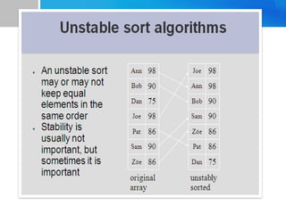
Sorting Order and Stability in Sorting.
Concept of Internal and External Sorting.
Bubble Sort,
Insertion Sort,
Selection Sort,
Quick Sort and
Merge Sort,
Radix Sort, and
Shell Sort,
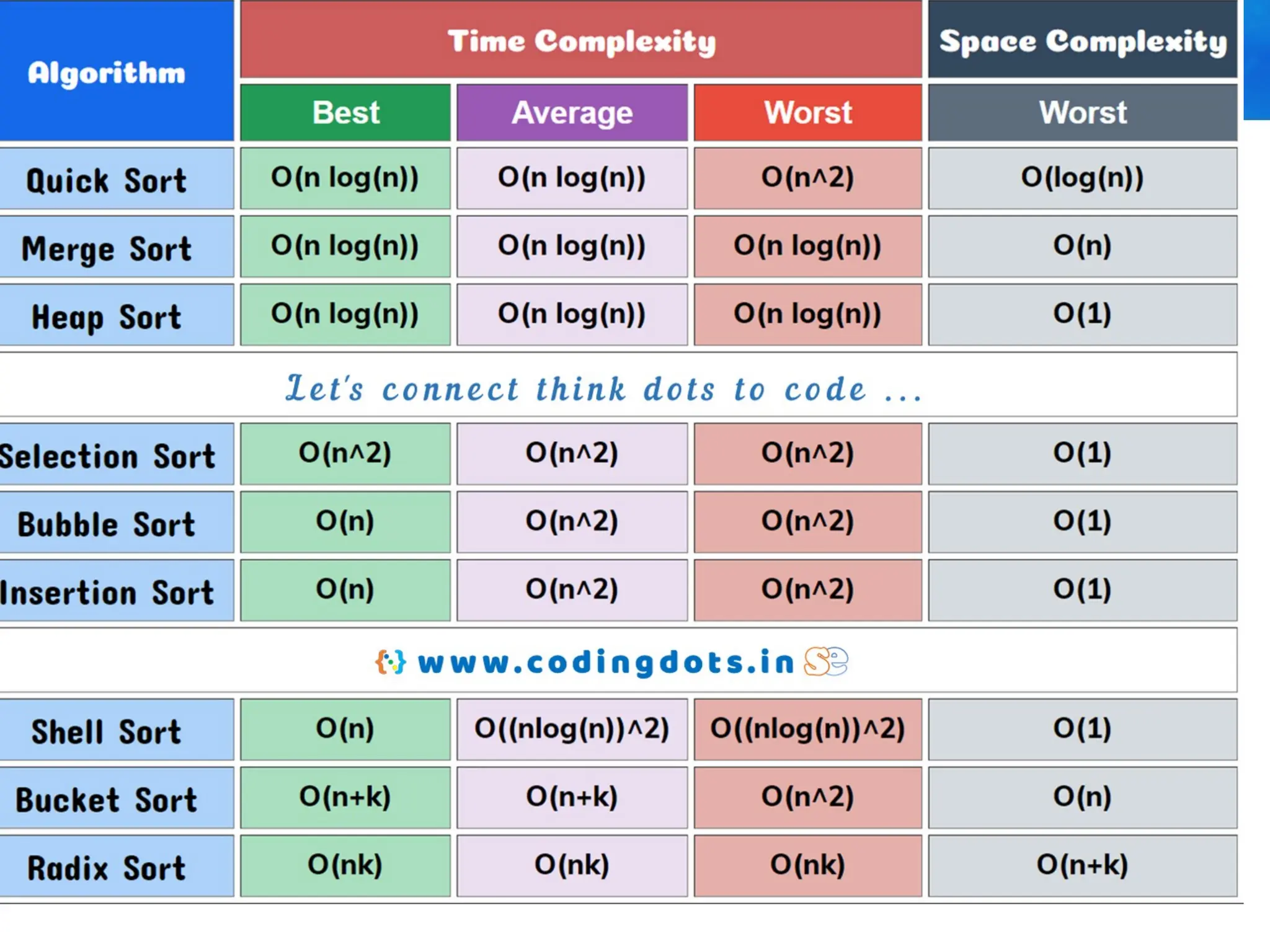
External Sorting, Time complexity analysis of Sorting Algorithms.
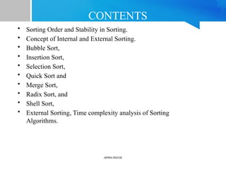
CONTENTS
• Sorting Orderand Stability in Sorting.
• Concept of Internal and External Sorting.
• Bubble Sort,
• Insertion Sort,
• Selection Sort,
• Quick Sort and
• Merge Sort,
• Radix Sort, and
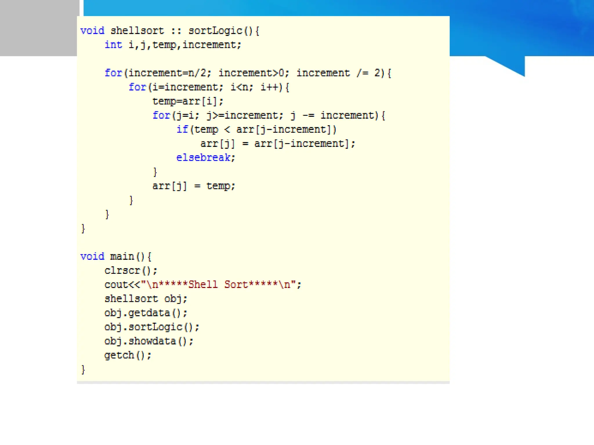
• Shell Sort,
• External Sorting, Time complexity analysis of Sorting
Algorithms.
JSPM's RSCOE
3.
Sequential Search
• Tosearch the key ‘22’:
int SeqSearch(int a[], int n, key)
{
int i;
for (i=0; i<n && a[i] != key; i++)
;
if (i >= n)
return -1;
return i;
}
23
0
2
1
7
2
15
3
42
4
12
5
The search makes n key comparisons when it is unsuccessful.
4.
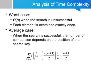
Analysis of TimeComplexity
• Worst case:
– O(n) when the search is unsuccessful.
– Each element is examined exactly once.
• Average case:
– When the search is successful, the number of
comparison depends on the position of the
search key.
2
1
1
2
)
1
(
1
n
n
n
n
n
i
n
i
5.
Binary Search
int BinarySearch(inta[], int n, in key)
{
int left = 0, right = n-1;
while (left <= right)
{
int middle = (left + right) / 2;
if (key < a[middle]) right = middle - 1;
else if (key > a[middle]) left = middle + 1;
else return middle;
}
return -1;
}
2
0
7
1
12
2
15
3
23
4
42
5
left right
middle
To find 23, middle
found.
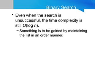
6.
Binary Search
• Evenwhen the search is
unsuccessful, the time complexity is
still O(log n).
– Something is to be gained by maintaining
the list in an order manner.
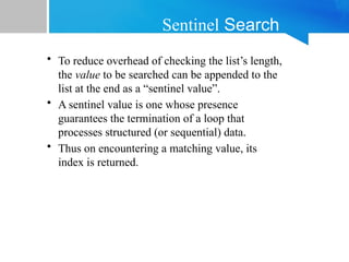
7.
Sentinel Search
• Toreduce overhead of checking the list’s length,
the value to be searched can be appended to the
list at the end as a “sentinel value”.
• A sentinel value is one whose presence
guarantees the termination of a loop that
processes structured (or sequential) data.
• Thus on encountering a matching value, its
index is returned.
Sorting
Sorting is theoperation of arranging the
records of a table according to the key value of
each record, or it can be defined as the process
of converting an unordered set of elements to
an ordered set.
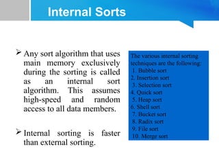
Internal Sorts
Anysort algorithm that uses
main memory exclusively
during the sorting is called
as an internal sort
algorithm. This assumes
high-speed and random
access to all data members.
Internal sorting is faster
than external sorting.
The various internal sorting
techniques are the following:
1. Bubble sort
2. Insertion sort
3. Selection sort
4. Quick sort
5. Heap sort
6. Shell sort
7. Bucket sort
8. Radix sort
9. File sort
10. Merge sort
13.
External sorts
Anysort algorithm that uses external memory,
such as tape or disk, during the sorting is called as
an external sort algorithm.
Merge sort uses external memory.
14.
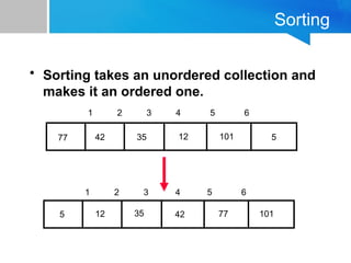
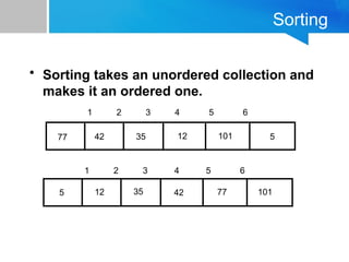
Sorting
• Sorting takesan unordered collection and
makes it an ordered one.
5
12
35
42
77 101
1 2 3 4 5 6
5 12 35 42 77 101
1 2 3 4 5 6
15.
Sorting an Arrayof Integers
• Example:
we are
given an
array of
six
integers
that we
want to
sort from
smallest
to largest
0
10
20
30
40
50
60
70
[1] [2] [3] [4] [5] [6]
[0] [1] [2] [3] [4] [5]
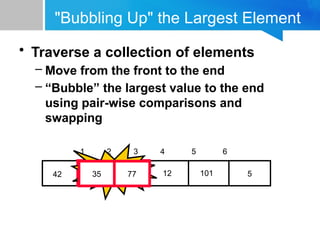
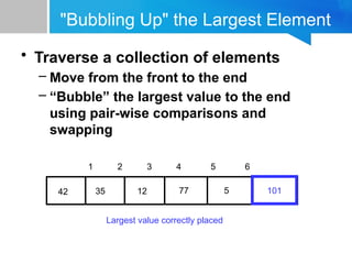
"Bubbling Up" theLargest Element
• Traverse a collection of elements
– Move from the front to the end
– “Bubble” the largest value to the end
using pair-wise comparisons and
swapping
5
12
35
42
77 101
1 2 3 4 5 6
20.
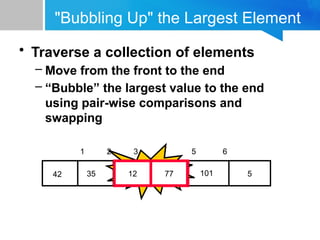
"Bubbling Up" theLargest Element
• Traverse a collection of elements
– Move from the front to the end
– “Bubble” the largest value to the end
using pair-wise comparisons and
swapping
5
12
35
42
77 101
1 2 3 4 5 6
Swap
42 77
21.
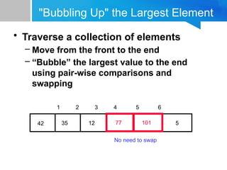
"Bubbling Up" theLargest Element
• Traverse a collection of elements
– Move from the front to the end
– “Bubble” the largest value to the end
using pair-wise comparisons and
swapping
5
12
35
77
42 101
1 2 3 4 5 6
Swap
35 77
22.
"Bubbling Up" theLargest Element
• Traverse a collection of elements
– Move from the front to the end
– “Bubble” the largest value to the end
using pair-wise comparisons and
swapping
5
12
77
35
42 101
1 2 3 4 5 6
Swap
12 77
23.
"Bubbling Up" theLargest Element
• Traverse a collection of elements
– Move from the front to the end
– “Bubble” the largest value to the end
using pair-wise comparisons and
swapping
5
77
12
35
42 101
1 2 3 4 5 6
No need to swap
24.
"Bubbling Up" theLargest Element
• Traverse a collection of elements
– Move from the front to the end
– “Bubble” the largest value to the end
using pair-wise comparisons and
swapping
5
77
12
35
42 101
1 2 3 4 5 6
Swap
5 101
25.
"Bubbling Up" theLargest Element
• Traverse a collection of elements
– Move from the front to the end
– “Bubble” the largest value to the end
using pair-wise comparisons and
swapping
77
12
35
42 5
1 2 3 4 5 6
101
Largest value correctly placed
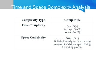
Time and SpaceComplexity Analysis
Complexity Type Complexity
Time Complexity Best: O(n)
Average: O(n^2)
Worst: O(n^2)
Space Complexity Worst: O(1)
Bubble Sort only needs a constant
amount of additional space during
the sorting process.
0
10
20
30
40
50
60
70
[1] [2] [3][4] [5] [6]
The Insertion Sort Algorithm
• The
Insertion
Sort
algorithm
also views
the array as
having a
sorted side
and an
unsorted
side.
[0] [1] [2] [3] [4] [5]
31.
0
10
20
30
40
50
60
70
[1] [2] [3][4] [5] [6]
The Insertion Sort Algorithm
• The sorted
side starts
with just
the first
element,
which is
not
necessarily
the
smallest
element. 0
10
20
30
40
50
60
70
[1] [2] [3] [4] [5] [6]
[0] [1] [2] [3] [4] [5]
Sorted side Unsorted side
32.
0
10
20
30
40
50
60
70
[1] [2] [3][4] [5] [6]
The Insertion Sort Algorithm
• The
sorted
side
grows by
taking the
front
element
from the
unsorted
side... 0
10
20
30
40
50
60
70
[1] [2] [3] [4] [5] [6]
[0] [1] [2] [3] [4] [5]
Sorted side Unsorted side
33.
0
10
20
30
40
50
60
70
[1] [2] [3][4] [5] [6]
The Insertion Sort Algorithm
• ...and
inserting it
in the
place that
keeps the
sorted
side
arranged
from
small to
large.
0
10
20
30
40
50
60
70
[1] [2] [3] [4] [5] [6]
[0] [1] [2] [3] [4] [5]
Sorted side Unsorted side
0
10
20
30
40
50
60
70
[1] [2] [3][4] [5] [6]
The Insertion Sort Algorithm
• Sometime
s we are
lucky and
the new
inserted
item
doesn't
need to
move at
all.
0
10
20
30
40
50
60
70
[1] [2] [3] [4] [5] [6]
[0] [1] [2] [3] [4] [5]
Sorted side Unsorted side
36.
0
10
20
30
40
50
60
70
[1] [2] [3][4] [5] [6]
The Insertionsort Algorithm
• Sometime
s we are
lucky
twice in a
row.
0
10
20
30
40
50
60
70
[1] [2] [3] [4] [5] [6]
[0] [1] [2] [3] [4] [5]
Sorted side Unsorted side
37.
0
10
20
30
40
50
60
70
[1] [2] [3][4] [5] [6]
How to Insert One Element
Copy the
new
element
to a
separate
location.
0
10
20
30
40
50
60
70
[1] [2] [3] [4] [5] [6]
0
10
20
30
40
50
60
70
[1] [2] [3] [4] [5] [6]
[0] [1] [2] [3] [4] [5]
Sorted side Unsorted side
38.
0
10
20
30
40
50
60
70
[1] [2] [3][4] [5] [6]
How to Insert One Element
Shift
elements
in the
sorted
side,
creating
an open
space for
the new
element.
0
10
20
30
40
50
60
70
[1] [2] [3] [4] [5] [6]
0
10
20
30
40
50
60
70
[1] [2] [3] [4] [5] [6]
[0] [1] [2] [3] [4] [5]
39.
0
10
20
30
40
50
60
70
[1] [2] [3][4] [5] [6]
0
10
20
30
40
50
60
70
[1] [2] [3] [4] [5] [6]
How to Insert One Element
Shift
elements
in the
sorted
side,
creating
an open
space for
the new
element.
0
10
20
30
40
50
60
70
[1] [2] [3] [4] [5] [6]
0
10
20
30
40
50
60
70
[1] [2] [3] [4] [5] [6]
[0] [1] [2] [3] [4] [5]
0
10
20
30
40
50
60
70
[1] [2] [3][4] [5] [6]
0
10
20
30
40
50
60
70
[1] [2] [3] [4] [5] [6]
How to Insert One Element
...until you
reach the
location
for the
new
element.
0
10
20
30
40
50
60
70
[1] [2] [3] [4] [5] [6]
0
10
20
30
40
50
60
70
[1] [2] [3] [4] [5] [6]
[0] [1] [2] [3] [4] [5]
43.
0
10
20
30
40
50
60
70
[1] [2] [3][4] [5] [6]
0
10
20
30
40
50
60
70
[1] [2] [3] [4] [5] [6]
How to Insert One Element
Copy the
new
element
back into
the array,
at the
correct
location.
0
10
20
30
40
50
60
70
[1] [2] [3] [4] [5] [6]
[0] [1] [2] [3] [4] [5]
Sorted side Unsorted side
44.
0
10
20
30
40
50
60
70
[1] [2] [3][4] [5] [6]
How to Insert One Element
0
10
20
30
40
50
60
70
[1] [2] [3] [4] [5] [6]
• The last
element
must also
be
inserted.
Start by
copying
it...
[0] [1] [2] [3] [4] [5]
Sorted side Unsorted side
void insertion_sort (intdata[], int n)
{
int i, j;
int temp;
if(n < 2) return; // nothing to sort!!
for(i = 1; i < n; ++i)
{
// take next item at front of unsorted part of array
// and insert it in appropriate location in sorted part of array
temp = data[i];
for(j = i; data[j-1] > temp && j > 0; --j)
data[j] = data[j-1]; // shift element forward
data[j] = temp;
}
}
47.
Insertion Sort TimeAnalysis
• In O-notation, what is:
– Worst case running time for n items?
– Average case running time for n items?
• Steps of algorithm:
for i = 1 to n-1
take next key from unsorted part of array
insert in appropriate location in sorted part of array:
for j = i down to 0,
shift sorted elements to the right if key > key[i]
increase size of sorted array by 1
Outer loop:
O(n)
48.
Insertion Sort TimeAnalysis
• In O-notation, what is:
– Worst case running time for n items?
– Average case running time for n items?
• Steps of algorithm:
for i = 1 to n-1
take next key from unsorted part of array
insert in appropriate location in sorted part of array:
for j = i down to 0,
shift sorted elements to the right if key > key[i]
increase size of sorted array by 1
Outer loop:
O(n)
Inner loop:
O(n)
49.
template <class Item>
voidinsertion_sort(Item data[ ], size_t n)
{
size_t i, j;
Item temp;
if(n < 2) return; // nothing to sort!!
for(i = 1; i < n; ++i)
{
// take next item at front of unsorted part of array
// and insert it in appropriate location in sorted part of array
temp = data[i];
for(j = i; data[j-1] > temp and j > 0; --j)
data[j] = data[j-1]; // shift element forward
data[j] = temp;
}
}
O(n)
O(n)
50.
Insertion Sort TimeAnalysis
• Steps of algorithm:
for i = 1 to n-1
take next key from unsorted part of array
insert in appropriate location in sorted part of array:
for j = i down to 0,
shift sorted elements to the right if key > key[i]
increase size of sorted array by 1
51.
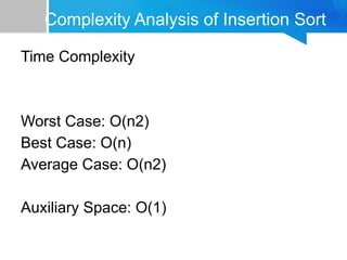
Complexity Analysis ofInsertion Sort
Time Complexity
Worst Case: O(n2)
Best Case: O(n)
Average Case: O(n2)
Auxiliary Space: O(1)
0
10
20
30
40
50
60
70
[1] [2] [3][4] [5] [6]
The Selection Sort Algorithm
• Swap the
smallest
entry with
the first
entry.
0
10
20
30
40
50
60
70
[1] [2] [3] [4] [5] [6]
[0] [1] [2] [3] [4] [5]
55.
0
10
20
30
40
50
60
70
[1] [2] [3][4] [5] [6]
The Selection Sort Algorithm
• Swap the
smallest
entry with
the first
entry.
0
10
20
30
40
50
60
70
[1] [2] [3] [4] [5] [6]
[0] [1] [2] [3] [4] [5]
56.
0
10
20
30
40
50
60
70
[1] [2] [3][4] [5] [6]
The Selection Sort Algorithm
• Part of the
array is
now
sorted.
0
10
20
30
40
50
60
70
[1] [2] [3] [4] [5] [6]
Sorted side Unsorted side
[0] [1] [2] [3] [4] [5]
57.
0
10
20
30
40
50
60
70
[1] [2] [3][4] [5] [6]
0
10
20
30
40
50
60
70
[1] [2] [3] [4] [5] [6]
The Selection Sort Algorithm
• Find the
smallest
element in
the
unsorted
side.
Sorted side Unsorted side
[0] [1] [2] [3] [4] [5]
58.
0
10
20
30
40
50
60
70
[1] [2] [3][4] [5] [6]
0
10
20
30
40
50
60
70
[1] [2] [3] [4] [5] [6]
The Selection Sort Algorithm
• Swap with
the front
of the
unsorted
side.
Sorted side Unsorted side
[0] [1] [2] [3] [4] [5]
59.
0
10
20
30
40
50
60
70
[1] [2] [3][4] [5] [6]
0
10
20
30
40
50
60
70
[1] [2] [3] [4] [5] [6]
The Selection Sort Algorithm
• We have
increased
the size of
the sorted
side by
one
element.
Sorted side Unsorted side
[0] [1] [2] [3] [4] [5]
60.
0
10
20
30
40
50
60
70
[1] [2] [3][4] [5] [6]
0
10
20
30
40
50
60
70
[1] [2] [3] [4] [5] [6]
The Selection Sort Algorithm
• The
process
continues.
..
Sorted side Unsorted side
Smallest
from
unsorted
[0] [1] [2] [3] [4] [5]
61.
0
10
20
30
40
50
60
70
[1] [2] [3][4] [5] [6]
0
10
20
30
40
50
60
70
[1] [2] [3] [4] [5] [6]
The Selection Sort Algorithm
• The
process
continues.
..
Sorted side Unsorted side
[0] [1] [2] [3] [4] [5]
Swap
with
front
62.
0
10
20
30
40
50
60
70
[1] [2] [3][4] [5] [6]
0
10
20
30
40
50
60
70
[1] [2] [3] [4] [5] [6]
The Selection Sort Algorithm
• The
process
continues.
..
Sorted side Unsorted side
Sorted side
is bigger
[0] [1] [2] [3] [4] [5]
63.
0
10
20
30
40
50
60
70
[1] [2] [3][4] [5] [6]
0
10
20
30
40
50
60
70
[1] [2] [3] [4] [5] [6]
The Selection Sort Algorithm
• The process
keeps adding
one more
number to the
sorted side.
• The sorted
side has the
smallest
numbers,
arranged from
small to large.
Sorted side Unsorted side
[0] [1] [2] [3] [4] [5]
64.
0
10
20
30
40
50
60
70
[1] [2] [3][4] [5] [6]
0
10
20
30
40
50
60
70
[1] [2] [3] [4] [5] [6]
The Selection Sort Algorithm
• We can stop
when the
unsorted
side has just
one number,
since that
number must
be the
largest
number.
[0] [1] [2] [3] [4] [5]
Sorted side Unsorted side
65.
0
10
20
30
40
50
60
70
[1] [2] [3][4] [5] [6]
The Selection Sort Algorithm
• The array is
now sorted.
• We
repeatedly
selected the
smallest
element, and
moved this
element to
the front of
the unsorted [0] [1] [2] [3] [4] [5]
66.
void selectionsort(int arr[],int n)
{
int i, j, min_idx;
// One by one move boundary of
// unsorted subarray
for (i = 0; i < n-1; i++)
{
// Find the minimum element in
// unsorted array
min_idx = i;
for (j = i+1; j < n; j++)
if (arr[j] < arr[min_idx])
min_idx = j;
// Swap the found minimum element
// with the first element
int temp = arr[min_idx];
arr[min_idx] = arr[i];
arr[i] = temp;
} }
67.
Selection Time SortAnalysis
• Steps of algorithm:
for i = 1 to n-1
find smallest key in unsorted part of array
swap smallest item to front of unsorted array
decrease size of unsorted array by 1
68.
template <class Item>
voidselection_sort(Item data[ ], size_t n)
{
size_t i, j, smallest;
Item temp;
if(n < 2) return; // nothing to sort!!
for(i = 0; i < n-1 ; ++i)
{
// find smallest in unsorted part of array
smallest = i;
for(j = i+1; j < n; ++j)
if(data[smallest] > data[j]) smallest = j;
// put it at front of unsorted part of array (swap)
temp = data[i];
data[i] = data[smallest];
data[smallest] = temp;
}
}
Outer loop:
O(n)
69.
template <class Item>
voidselection_sort(Item data[ ], size_t n)
{
size_t i, j, smallest;
Item temp;
if(n < 2) return; // nothing to sort!!
for(i = 0; i < n-1 ; ++i)
{
// find smallest in unsorted part of array
smallest = i;
for(j = i+1; j < n; ++j)
if(data[smallest] > data[j]) smallest = j;
// put it at front of unsorted part of array (swap)
temp = data[i];
data[i] = data[smallest];
data[smallest] = temp;
}
}
Outer loop:
O(n)
Inner loop:
O(n)
70.
Selection Time SortAnalysis
• Steps of algorithm:
for i = 1 to n-1 O(n)
find smallest key in unsorted part of array O(n)
swap smallest item to front of unsorted array
decrease size of unsorted array by 1
• Selection sort analysis: O(n2
)
71.
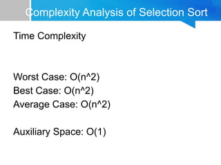
Complexity Analysis ofSelection Sort
Time Complexity
Worst Case: O(n^2)
Best Case: O(n^2)
Average Case: O(n^2)
Auxiliary Space: O(1)
72.
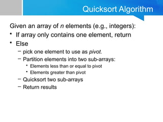
Quicksort Algorithm
Given anarray of n elements (e.g., integers):
• If array only contains one element, return
• Else
– pick one element to use as pivot.
– Partition elements into two sub-arrays:
• Elements less than or equal to pivot
• Elements greater than pivot
– Quicksort two sub-arrays
– Return results
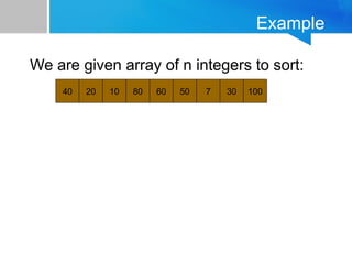
Pick Pivot Element
Thereare a number of ways to pick the pivot element.
In this example, we will use the first element in the
array:
40 20 10 80 60 50 7 30 100
75.
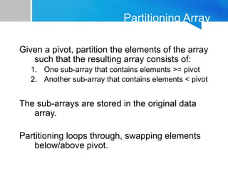
Partitioning Array
Given apivot, partition the elements of the array
such that the resulting array consists of:
1. One sub-array that contains elements >= pivot
2. Another sub-array that contains elements < pivot
The sub-arrays are stored in the original data
array.
Partitioning loops through, swapping elements
below/above pivot.
40 20 1080 60 50 7 30 100
pivot_index = 0
[0] [1] [2] [3] [4] [5] [6] [7] [8]
i j
1. While data[i] <= data[pivot]
++i
2. While data[j] > data[pivot]
--j
3. If i < j
swap data[i] and data[j]
83.
40 20 1030 60 50 7 80 100
pivot_index = 0
[0] [1] [2] [3] [4] [5] [6] [7] [8]
i j
1. While data[i] <= data[pivot]
++i
2. While data[j] > data[pivot]
--j
3. If i< j
swap data[i] and data[j]
84.
40 20 1030 60 50 7 80 100
pivot_index = 0
[0] [1] [2] [3] [4] [ 5] [6] [7] [8]
i j
1. While data[i] <= data[pivot]
++i
2. While data[j] > data[pivot]
--j
3. If i < j
swap data[i] and data[j]
4. While j > i go to 1.
85.
40 20 1030 60 50 7 80 100
pivot_index = 0
[0] [1] [2] [3] [4] [5] [6] [7] [8]
i j
1. While data[i] <= data[pivot]
++i
2. While data[j] > data[pivot]
--j
3. If i<j
swap data[i] and data[j]
4. While j> i, go to 1.
86.
40 20 1030 60 50 7 80 100
pivot_index = 0
[0] [1] [2] [3] [4] [5] [6] [7] [8]
i j
1. While data[i] <= data[pivot]
++i
2. While data[j] > data[pivot]
--j
3. If i< j
swap data[i] and data[j]
4. While j > i, go to 1.
87.
40 20 1030 60 50 7 80 100
pivot_index = 0
[0] [1] [2] [3] [4] [5] [6] [7] [8]
i j
1. While data[i] <= data[pivot]
++i
2. While data[j] > data[pivot]
--j
3. If i < j
swap data[i] and data[j]
4. While j > i, go to 1.
88.
40 20 1030 60 50 7 80 100
pivot_index = 0
[0] [1] [2] [3] [4] [5] [6] [7] [8]
i j
1. While data[i] <= data[pivot]
++i
2. While data[j] > data[pivot]
--j
3. If i < j
swap data[i] and data[j]
4. While j > i, go to 1.
89.
40 20 1030 60 50 7 80 100
pivot_index = 0
[0] [1] [2] [3] [4] [5] [6] [7] [8]
i j
1. While data[i] <= data[pivot]
++i
2. While data[j] > data[pivot]
--j
3. If i < j
swap data[i] and data[j]
4. While j> i, go to 1.
90.
1. While data[i]<= data[pivot]
++i
2. While data[j] > data[pivot]
--j
3. If i < j
swap data[i] and data[j]
4. While j> i, go to 1.
40 20 10 30 7 50 60 80 100
pivot_index = 0
[0] [1] [2] [3] [4] [5] [6] [7] [8]
i j
91.
1. While data[i]<= data[pivot]
++i
2. While data[j] > data[pivot]
--j
3. If i< j
swap data[i] and data[j]
4. While j> i, go to 1.
40 20 10 30 7 50 60 80 100
pivot_index = 0
[0] [1] [2] [3] [4] [5] [6] [7] [8]
i j
92.
1. While data[i]<= data[pivot]
++i
2. While data[j] > data[pivot]
--j
3. If i < j
swap data[i] and data[j]
4. While j > i, go to 1.
40 20 10 30 7 50 60 80 100
pivot_index = 0
[0] [1] [2] [3] [4] [5] [6] [7] [8]
i j
93.
1. While data[i]<= data[pivot]
++i
2. While data[j] > data[pivot]
--j
3. If i < j
swap data[i] and data[j]
4. While j > i, go to 1.
40 20 10 30 7 50 60 80 100
pivot_index = 0
[0] [1] [2] [3] [4] [5] [6] [7] [8]
i j
94.
1. While data[i]<= data[pivot]
++i
2. While data[j] > data[pivot]
--j
3. If i< j
swap data[i] and data[j]
4. While j > i, go to 1.
40 20 10 30 7 50 60 80 100
pivot_index = 0
[0] [1] [2] [3] [4] [5] [6] [7] [8]
i j
95.
1. While data[i]<= data[pivot]
++i
2. While data[j] > data[pivot]
--j
3. If i < j
swap data[i] and data[j]
4. While j > i, go to 1.
40 20 10 30 7 50 60 80 100
pivot_index = 0
[0] [1] [2] [3] [4] [5] [6] [7] [8]
i j
96.
1. While data[i]<= data[pivot]
++i
2. While data[j] > data[pivot]
--j
3. If i < j
swap data[i] and data[j]
4. While j > i, go to 1.
40 20 10 30 7 50 60 80 100
pivot_index = 0
[0] [1] [2] [3] [4] [5] [6] [7] [8]
i j
97.
1. While data[i]<= data[pivot]
++i
2. While data[j] > data[pivot]
--j
3. If i < j
swap data[i] and data[j]
4. While j > i, go to 1.
40 20 10 30 7 50 60 80 100
pivot_index = 0
[0] [1] [2] [3] [4] [5] [6] [7] [8]
i j
98.
1. While data[i]<= data[pivot]
++i
2. While data[j] > data[pivot]
--j
3. If i<j
swap data[i] and data[j]
4. While j > i, go to 1.
40 20 10 30 7 50 60 80 100
pivot_index = 0
[0] [1] [2] [3] [4] [5] [6] [7] [8]
i j
99.
1. While data[i]<= data[pivot]
++I
2. While data[j] > data[pivot]
--j
3. If i < j
swap data[i] and data[j]
4. While j > i, go to 1.
5. Swap data[j] and data[pivot_index]
40 20 10 30 7 50 60 80 100
pivot_index = 0
[0] [1] [2] [3] [4] [5] [6] [7] [8]
i j
100.
1. While data[i]<= data[pivot]
++I
2. While data[j] > data[pivot]
--j
3. If i<j
swap data[i] and data[j]
4. While j > i, go to 1.
5. Swap data[j] and
data[pivot_index]
7 20 10 30 40 50 60 80 100
pivot_index = 4
[0] [1] [2] [3] [4] [5] [6] [7] [8]
i j
Sorting
• Sorting takesan unordered collection and
makes it an ordered one.
5
12
35
42
77 101
1 2 3 4 5 6
5 12 35 42 77 101
1 2 3 4 5 6
106.
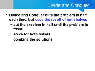
Divide and Conquer
•Divide and Conquer cuts the problem in half
each time, but uses the result of both halves:
– cut the problem in half until the problem is
trivial
– solve for both halves
– combine the solutions
107.
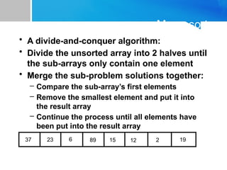
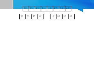
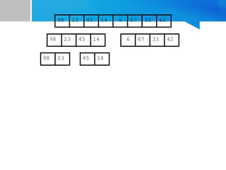
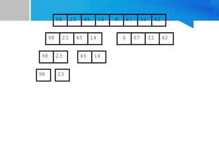
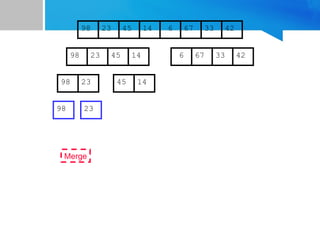
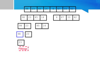
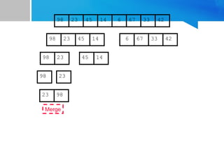
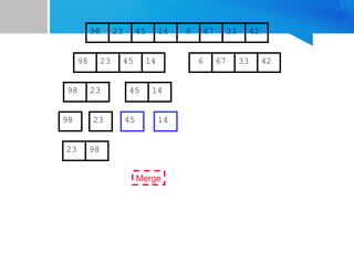
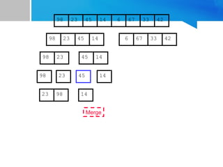
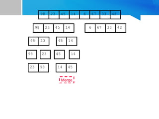
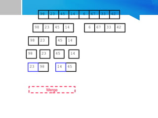
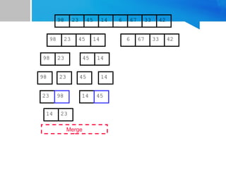
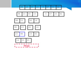
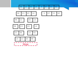
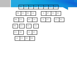
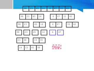
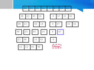
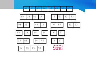
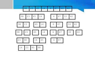
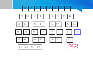
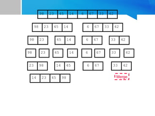
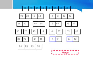
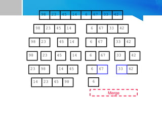
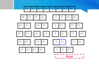
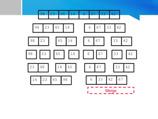
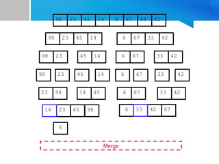
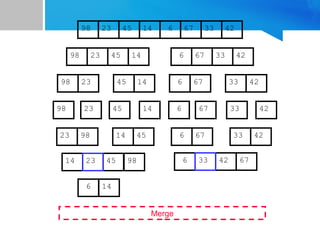
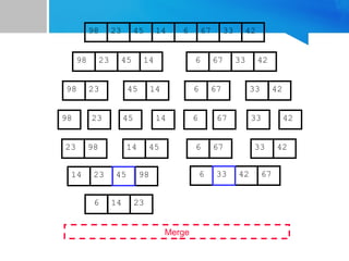
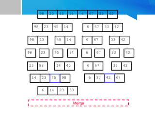
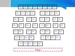
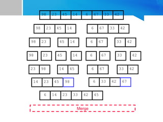
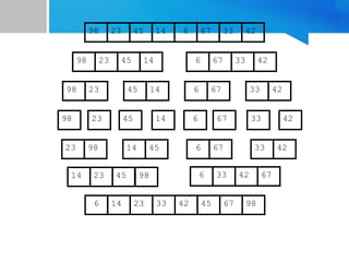
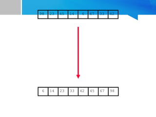
Mergesort
• A divide-and-conqueralgorithm:
• Divide the unsorted array into 2 halves until
the sub-arrays only contain one element
• Merge the sub-problem solutions together:
– Compare the sub-array’s first elements
– Remove the smallest element and put it into
the result array
– Continue the process until all elements have
been put into the result array
37 23 6 89 15 12 2 19
// The subarrayto be sorted is in the index range [left-right]
void mergeSort(int arr[], int left, int right) {
if (left < right) {
// Calculate the midpoint
int mid = (right + left) / 2;
// Sort first and second halves
mergeSort(arr, left, mid);
mergeSort(arr, mid + 1, right);
// Merge the sorted halves
merge(arr, left, mid, right);
}
150.
void merge(int arr[],int left, int mid, int right) {
int i, j, k;
int n1 = mid - left + 1;
int n2 = right - mid;
// Create temporary arrays
int leftArr[n1], rightArr[n2];
// Copy data to temporary arrays
for (i = 0; i < n1; i++)
leftArr[i] = arr[left + i];
for (j = 0; j < n2; j++)
rightArr[j] = arr[mid + 1 + j];
151.
// Merge thetemporary arrays back
into arr[left..right]
i = 0;
j = 0;
k = left;
while (i < n1 && j < n2) {
if (leftArr[i] <= rightArr[j]) {
arr[k] = leftArr[i];
i++;
}
else {
arr[k] = rightArr[j];
j++;
}
k++;
}
// Copy the remaining elements of leftArr[], if any
while (i < n1) {
arr[k] = leftArr[i];
i++;
k++;
}
// Copy the remaining elements of rightArr[], if any
while (j < n2) {
arr[k] = rightArr[j];
j++;
k++;
}
}
152.
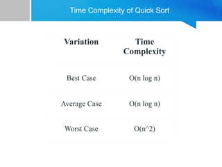
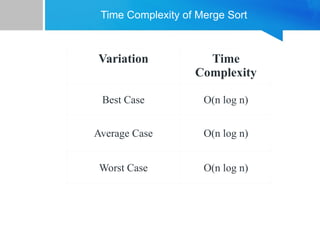
Time Complexity ofMerge Sort
Variation Time
Complexity
Best Case O(n log n)
Average Case O(n log n)
Worst Case O(n log n)
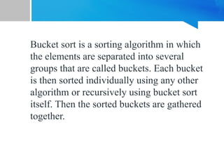
Bucket sort isa sorting algorithm in which
the elements are separated into several
groups that are called buckets. Each bucket
is then sorted individually using any other
algorithm or recursively using bucket sort
itself. Then the sorted buckets are gathered
together.
155.
Bucket Sort Algorithm:
Thealgorithm can be expressed as following:
1. Take the array then find the maximum and minimum elements of the array.
Find the range of each bucket.
Bucket range:((maximum element – minimum element)/number of elements)
2. Now insert the element into the bucket based on Bucket Index.
Bucket Index: floor(a[i]-minimum element)/range
3. Once the elements are inserted into each bucket, sort the elements within
each bucket using the insertion sort.
156.
Consider an arrayarr[] = {22, 72, 62, 32, 82, 142}
Range= (maximum-minimum) / number of elements
So, here the range will be given as: Range = (142 – 22)/6 = 20
Thus, the range of each bucket in bucket sort will be: 20 So, the buckets will
be as:
20-40; 40-60; 60-80; 80-100; 100-120; 120-140; 140-160
Bucket index = floor((a[i]-min)/range)
For 22, bucketindex = (22-22)/20 = 0.
For 72, bucketindex = (72-22)/20 = 2.5.
For 62, bucketindex = (62-22)/20 = 2.
For 32, bucketindex = (32-22)/20 = 0.5.
For 82, bucketindex = (82-22)/20 = 3.
For 142, bucketindex = (142-22)/20 = 6.
157.
Elements can beinserted into the bucket as:
0 -> 22 -> 32
1
2 -> 72 -> 62 (72 will be inserted before 62 as it appears first in the list).
3 -> 82
4
5
6 -> 142
Now sort the elements in each bucket using the insertion sort.
0 -> 22 -> 32
1
2 -> 62 -> 72
3 -> 82
4
5
6 -> 142
Now gather them together.
arr[] = {22, 32, 62, 72, 82, 142}
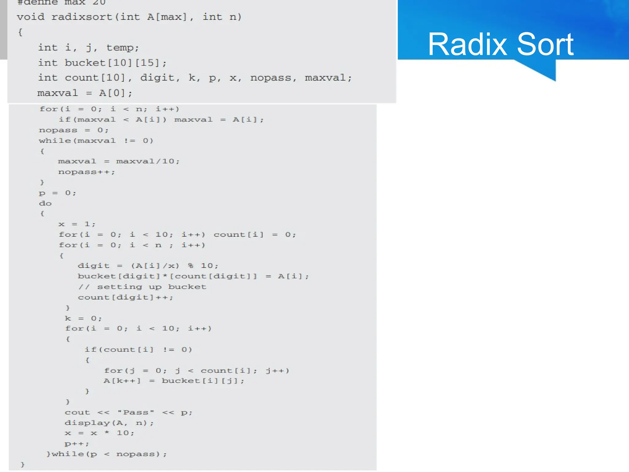
Radix Sort
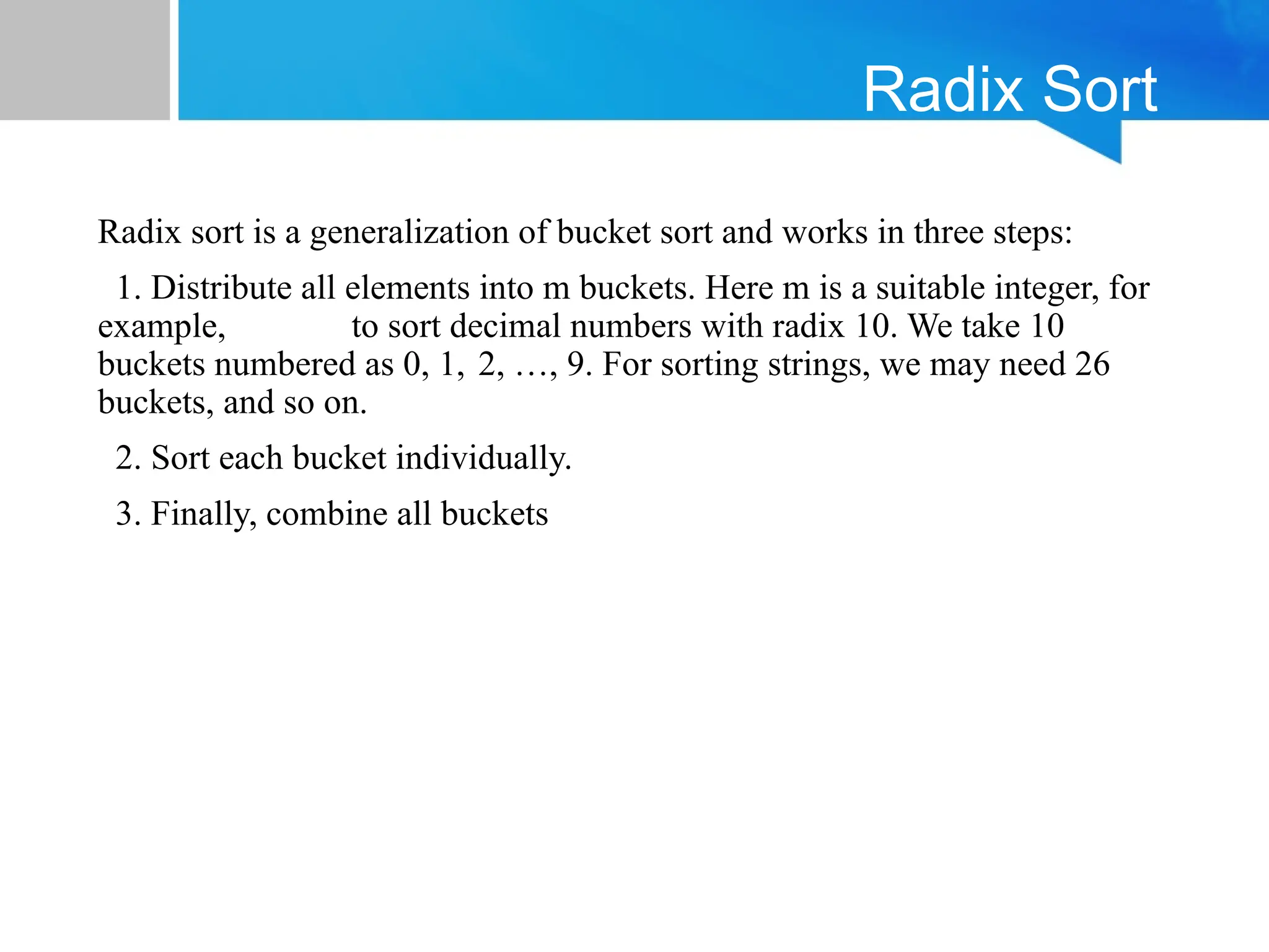
Radix sortis a generalization of bucket sort and works in three steps:
1. Distribute all elements into m buckets. Here m is a suitable integer, for
example, to sort decimal numbers with radix 10. We take 10
buckets numbered as 0, 1, 2, …, 9. For sorting strings, we may need 26
buckets, and so on.
2. Sort each bucket individually.
3. Finally, combine all buckets
160.
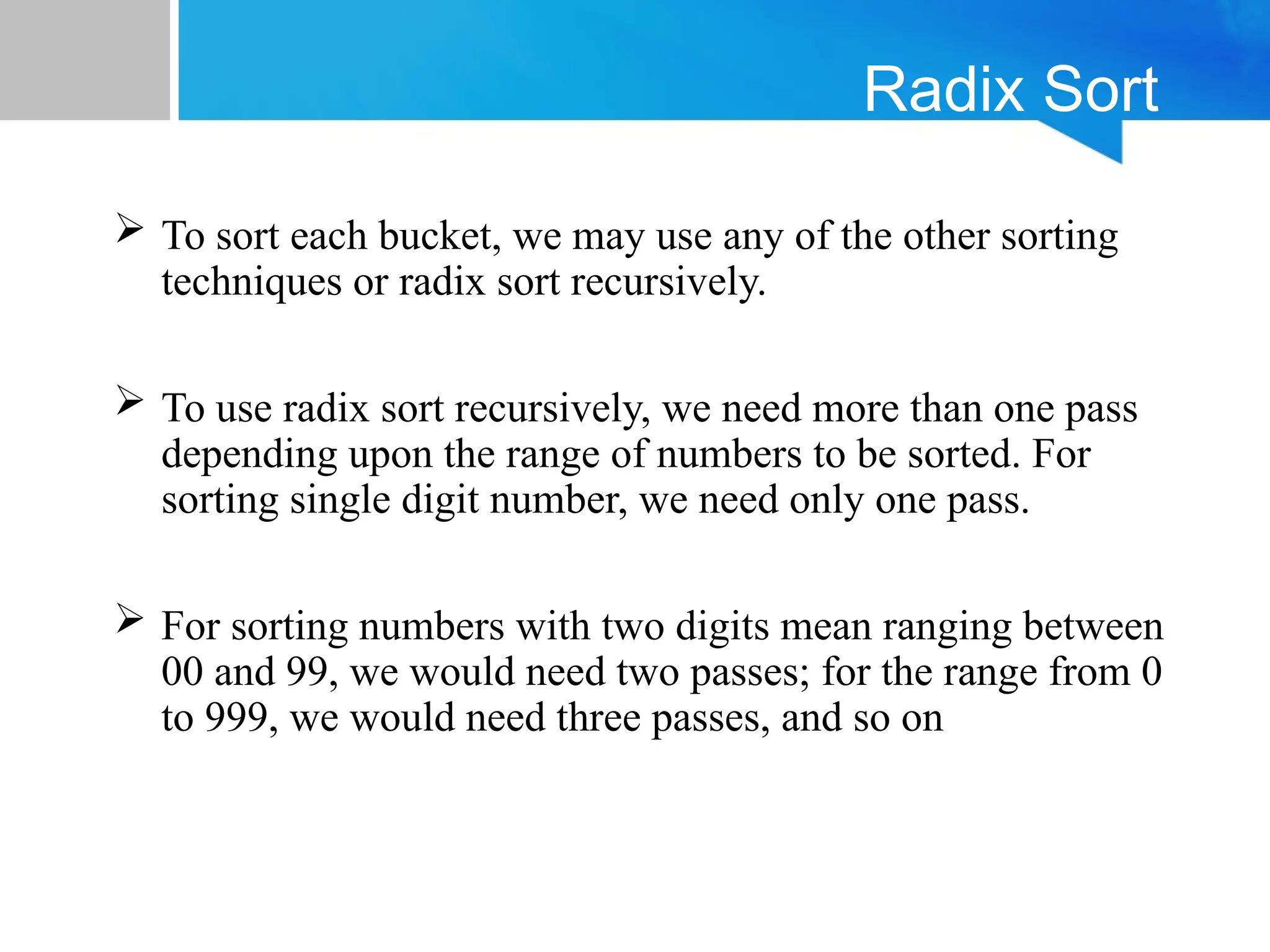
Radix Sort
Tosort each bucket, we may use any of the other sorting
techniques or radix sort recursively.
To use radix sort recursively, we need more than one pass
depending upon the range of numbers to be sorted. For
sorting single digit number, we need only one pass.
For sorting numbers with two digits mean ranging between
00 and 99, we would need two passes; for the range from 0
to 999, we would need three passes, and so on
161.
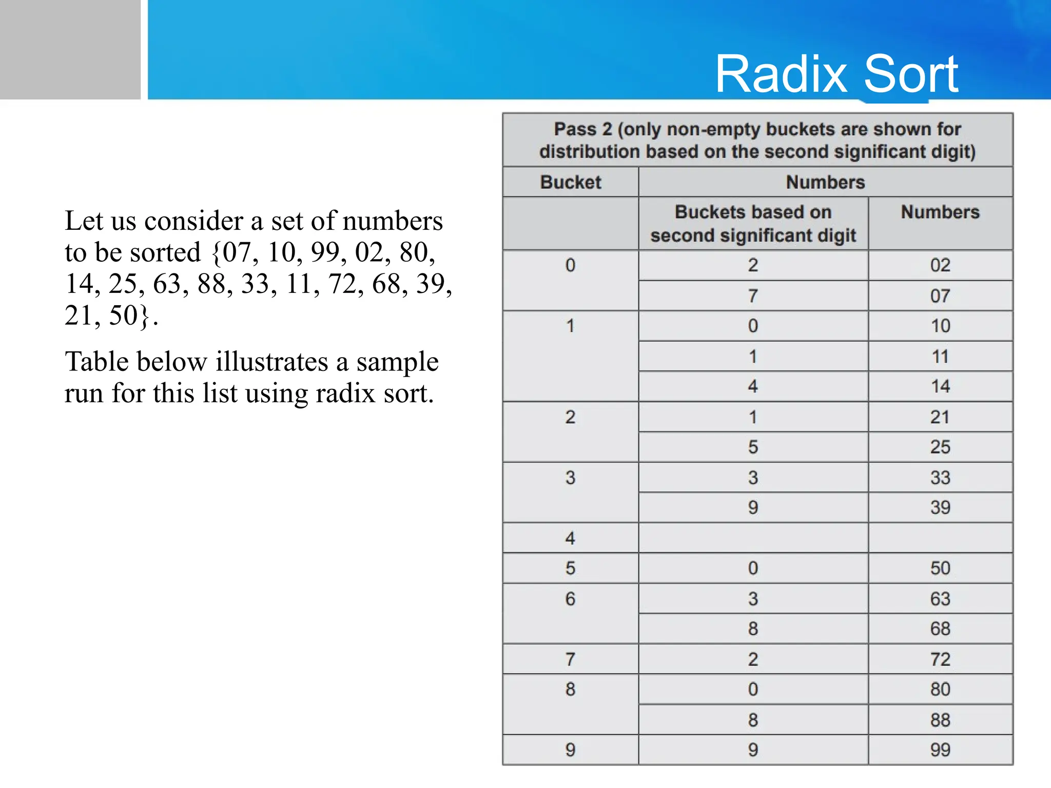
Radix Sort
Let usconsider a set of numbers
to be sorted {07, 10, 99, 02, 80,
14, 25, 63, 88, 33, 11, 72, 68, 39,
21, 50}.
Table below illustrates a sample
run for this list using radix sort.
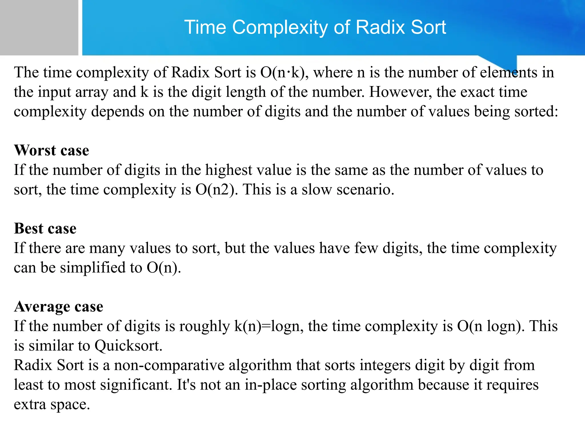
Time Complexity ofRadix Sort
The time complexity of Radix Sort is O(n k), where n is the number of elements in
⋅
the input array and k is the digit length of the number. However, the exact time
complexity depends on the number of digits and the number of values being sorted:
Worst case
If the number of digits in the highest value is the same as the number of values to
sort, the time complexity is O(n2). This is a slow scenario.
Best case
If there are many values to sort, but the values have few digits, the time complexity
can be simplified to O(n).
Average case
If the number of digits is roughly k(n)=logn, the time complexity is O(n logn). This
is similar to Quicksort.
Radix Sort is a non-comparative algorithm that sorts integers digit by digit from
least to most significant. It's not an in-place sorting algorithm because it requires
extra space.
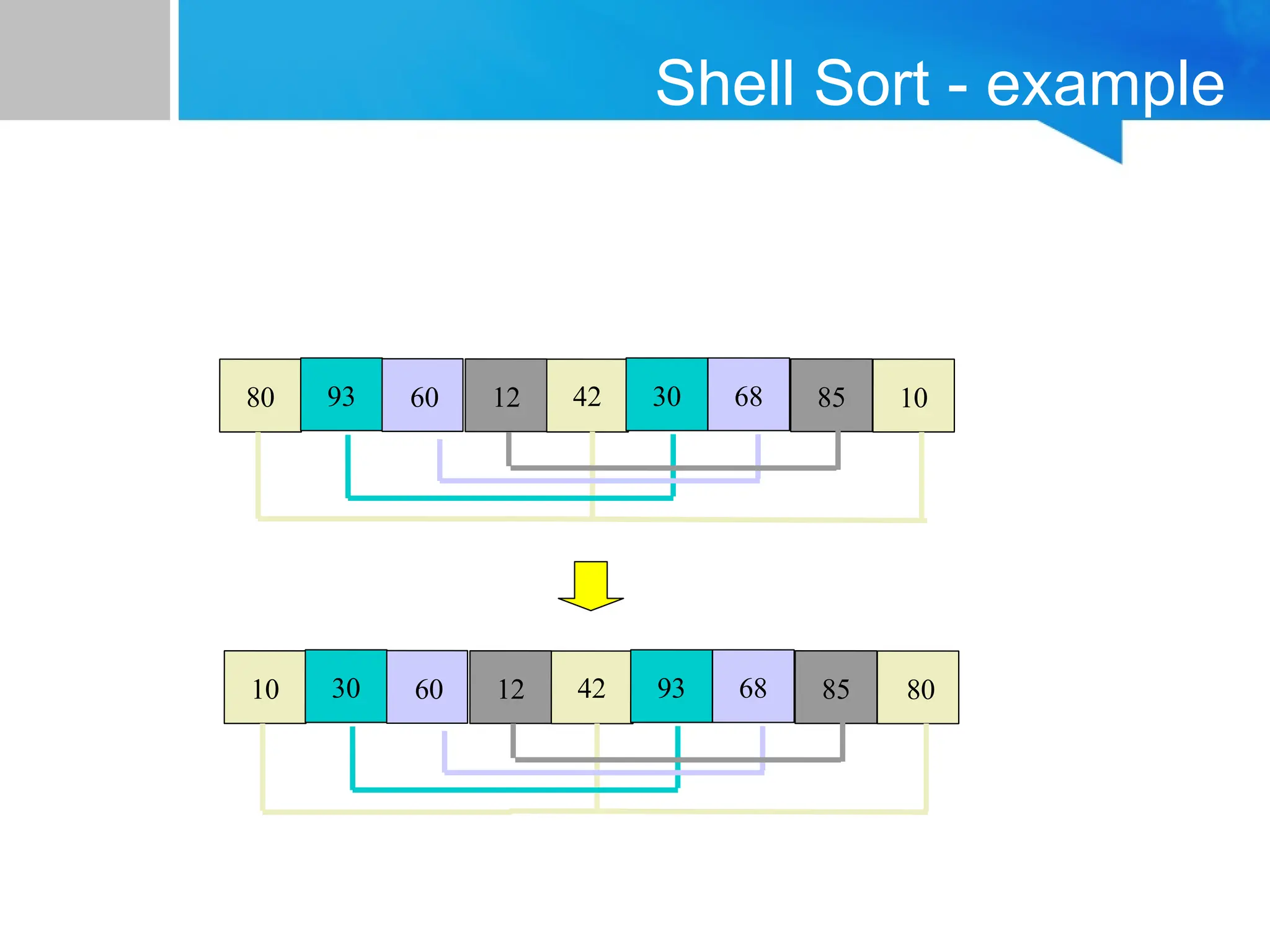
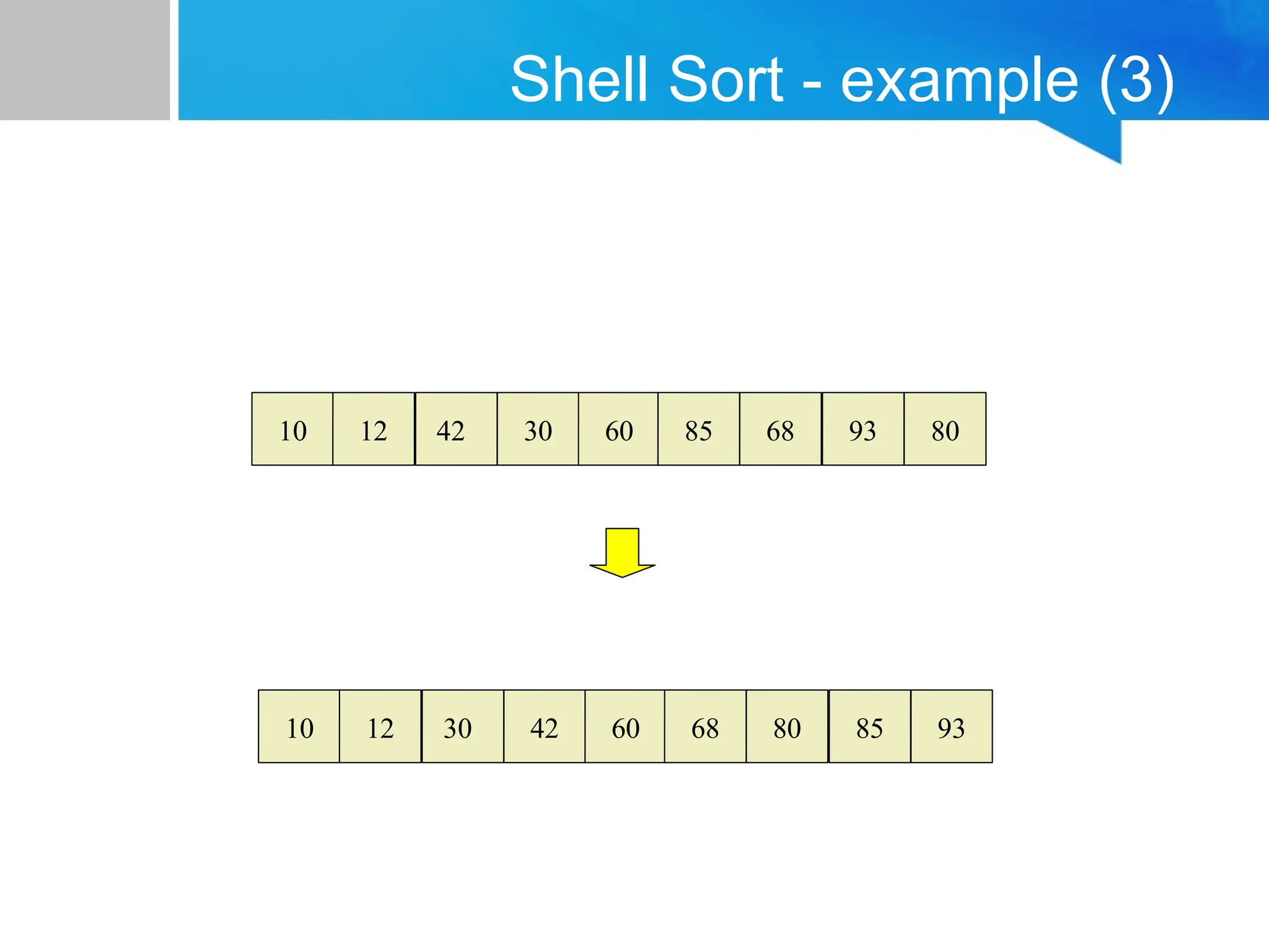
Shell Sort -GeneralDescription
•
Essentially a segmented insertion sort
– Divides an array into several smaller non-
contiguous segments
– The distance between successive elements in one
segment is called a gap.
– Each segment is sorted within itself using insertion
sort.
– Then resegment into larger segments (smaller
gaps) and repeat sort.
– Continue until only one segment (gap = 1) - final
sort finishes array sorting.
166.
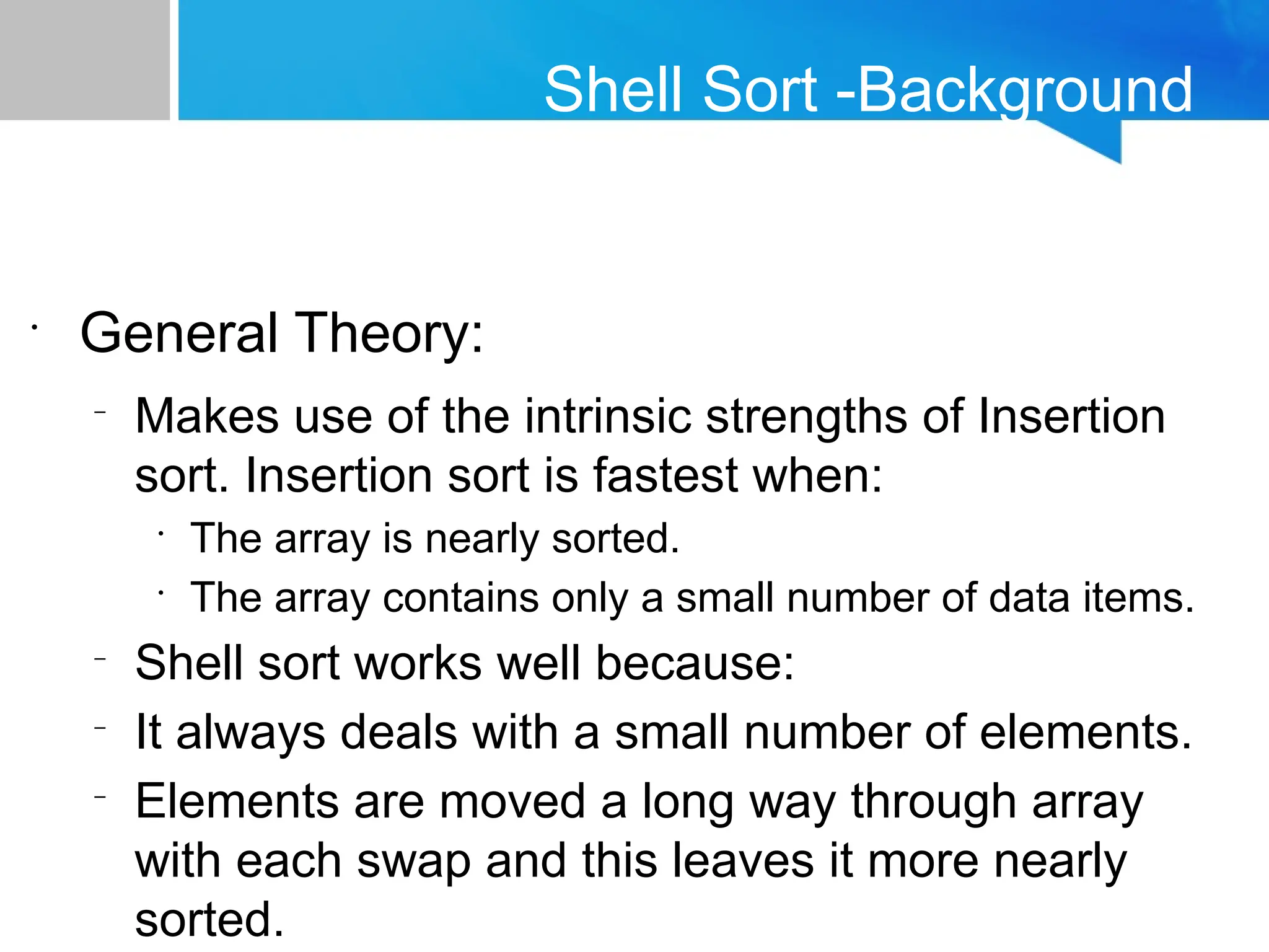
Shell Sort -Background
•
GeneralTheory:
–
Makes use of the intrinsic strengths of Insertion
sort. Insertion sort is fastest when:
•
The array is nearly sorted.
•
The array contains only a small number of data items.
–
Shell sort works well because:
–
It always deals with a small number of elements.
–
Elements are moved a long way through array
with each swap and this leaves it more nearly
sorted.
#15 The picture shows a graphical representation of an array which we will sort so that the smallest element ends up at the front, and the other elements increase to the largest at the end. The bar graph indicates the values which are in the array before sorting--for example the first element of the array contains the integer 45.
#30 Now we'll look at another sorting method called Insertionsort. The end result will be the same: The array will be sorted from smallest to largest. But the sorting method is different.
However, there are some common features. As with the Selectionsort, the Insertionsort algorithm also views the array as having a sorted side and an unsorted side, ...
#31 ...like this.
However, in the Selectionsort, the sorted side always contained the smallest elements of the array. In the Insertionsort, the sorted side will be sorted from small to large, but the elements in the sorted side will not necessarily be the smallest entries of the array.
Because the sorted side does not need to have the smallest entries, we can start by placing one element in the sorted side--we don't need to worry about sorting just one element. But we do need to worry about how to increase the number of elements that are in the sorted side.
#32 The basic approach is to take the front element from the unsorted side...
#33 ...and insert this element at the correct spot of the sorted side.
In this example, the front element of the unsorted side is 20. So the 20 must be inserted before the number 45 which is already in the sorted side.
#34 After the insertion, the sorted side contains two elements. These two elements are in order from small to large, although they are not the smallest elements in the array.
#35 Sometimes we are lucky and the newly inserted element is already in the right spot. This happens if the new element is larger than anything that's already in the array.
#37 The actual insertion process requires a bit of work that is shown here. The first step of the insertion is to make a copy of the new element. Usually this copy is stored in a local variable. It just sits off to the side, ready for us to use whenever we need it.
#38 After we have safely made a copy of the new element, we start shifting elements from the end of the sorted side. These elements are shifted rightward, to create an "empty spot" for our new element to be placed.
In this example we take the last element of the sorted side and shift it rightward one spot...
#39 ...like this.
Is this the correct spot for the new element? No, because the new element is smaller than the next element in the sorted section. So we continue shifting elements rightward...
#40 This is still not the correct spot for our new element, so we shift again...
#42 Finally, this is the correct location for the new element. In general there are two situations that indicate the "correct location" has been found:
1. We reach the front of the array (as happened here), or
2. We reached an element that is less than or equal to the new element.
#43 Once the correct spot is found, we copy the new element back into the array. The number of elements in the sorted side has increased by one.
#44 The last element of the array also needs to be inserted. Start by copying it to a safe location.
#53 The first sorting algorithm that we'll examine is called Selectionsort. It begins by going through the entire array and finding the smallest element. In this example, the smallest element is the number 8 at location [4] of the array.
#54 Once we have found the smallest element, that element is swapped with the first element of the array...
#55 ...like this.
The smallest element is now at the front of the array, and we have taken one small step toward producing a sorted array.
#56 At this point, we can view the array as being split into two sides: To the left of the dotted line is the "sorted side", and to the right of the dotted line is the "unsorted side". Our goal is to push the dotted line forward, increasing the number of elements in the sorted side, until the entire array is sorted.
#57 Each step of the Selectionsort works by finding the smallest element in the unsorted side. At this point, we would find the number 15 at location [5] in the unsorted side.
#58 This small element is swapped with the number at the front of the unsorted side, as shown here...
#59 ...and the effect is to increase the size of the sorted side by one element.
As you can see, the sorted side always contains the smallest numbers, and those numbers are sorted from small to large. The unsorted side contains the rest of the numbers, and those numbers are in no particular order.
#60 Again, we find the smallest entry in the unsorted side...
#61 ...and swap this element with the front of the unsorted side.
#62 The sorted side now contains the three smallest elements of the array.
#63 Here is the array after increasing the sorted side to four elements.
#64 And now the sorted side has five elements.
In fact, once the unsorted side is down to a single element, the sort is completed. At this point the 5 smallest elements are in the sorted side, and so the the one largest element is left in the unsorted side.
We are done...
#65 ...The array is sorted.
The basic algorithm is easy to state and also easy to program.
![Sequential Search
• To search the key ‘22’:
int SeqSearch(int a[], int n, key)
{
int i;
for (i=0; i<n && a[i] != key; i++)
;
if (i >= n)
return -1;
return i;
}
23
0
2
1
7
2
15
3
42
4
12
5
The search makes n key comparisons when it is unsuccessful.](https://image.slidesharecdn.com/datastructuressearchingandsorting-250503115212-17f1421f/85/Data-Structures_Searching-and-Sorting-pptx-3-320.jpg)
![Binary Search
int BinarySearch(int a[], int n, in key)
{
int left = 0, right = n-1;
while (left <= right)
{
int middle = (left + right) / 2;
if (key < a[middle]) right = middle - 1;
else if (key > a[middle]) left = middle + 1;
else return middle;
}
return -1;
}
2
0
7
1
12
2
15
3
23
4
42
5
left right
middle
To find 23, middle
found.](https://image.slidesharecdn.com/datastructuressearchingandsorting-250503115212-17f1421f/85/Data-Structures_Searching-and-Sorting-pptx-5-320.jpg)


![Sorting an Array of Integers
• Example:
we are
given an
array of
six
integers
that we
want to
sort from
smallest
to largest
0
10
20
30
40
50
60
70
[1] [2] [3] [4] [5] [6]
[0] [1] [2] [3] [4] [5]](https://image.slidesharecdn.com/datastructuressearchingandsorting-250503115212-17f1421f/85/Data-Structures_Searching-and-Sorting-pptx-15-320.jpg)


![void BubbleSort(int a[],n)
{
int i,j,temp;
for(i=1;i<n;i++)
for(j=0;j<n-i;j++)
if(a[j]>a[j+1])
{
temp=a[j];
a[j]=a[j+1];
a[j+1]=temp;
}
}](https://image.slidesharecdn.com/datastructuressearchingandsorting-250503115212-17f1421f/85/Data-Structures_Searching-and-Sorting-pptx-26-320.jpg)
![void BubbleSort(int a[],n)
{
int i,j,temp;
for(i=1;i<n;i++)
{ bool flag = false
for(j=0;j<n-i;j++)
{ if(a[j]>a[j+1])
{ flag = true
temp=a[j];
a[j]=a[j+1];
a[j+1]=temp;
}
}
if(!flag) break;
}
}
Optimized Bubble Sort](https://image.slidesharecdn.com/datastructuressearchingandsorting-250503115212-17f1421f/85/Data-Structures_Searching-and-Sorting-pptx-27-320.jpg)

![0
10
20
30
40
50
60
70
[1] [2] [3] [4] [5] [6]
The Insertion Sort Algorithm
• The
Insertion
Sort
algorithm
also views
the array as
having a
sorted side
and an
unsorted
side.
[0] [1] [2] [3] [4] [5]](https://image.slidesharecdn.com/datastructuressearchingandsorting-250503115212-17f1421f/85/Data-Structures_Searching-and-Sorting-pptx-30-320.jpg)
![0
10
20
30
40
50
60
70
[1] [2] [3] [4] [5] [6]
The Insertion Sort Algorithm
• The sorted
side starts
with just
the first
element,
which is
not
necessarily
the
smallest
element. 0
10
20
30
40
50
60
70
[1] [2] [3] [4] [5] [6]
[0] [1] [2] [3] [4] [5]
Sorted side Unsorted side](https://image.slidesharecdn.com/datastructuressearchingandsorting-250503115212-17f1421f/85/Data-Structures_Searching-and-Sorting-pptx-31-320.jpg)
![0
10
20
30
40
50
60
70
[1] [2] [3] [4] [5] [6]
The Insertion Sort Algorithm
• The
sorted
side
grows by
taking the
front
element
from the
unsorted
side... 0
10
20
30
40
50
60
70
[1] [2] [3] [4] [5] [6]
[0] [1] [2] [3] [4] [5]
Sorted side Unsorted side](https://image.slidesharecdn.com/datastructuressearchingandsorting-250503115212-17f1421f/85/Data-Structures_Searching-and-Sorting-pptx-32-320.jpg)
![0
10
20
30
40
50
60
70
[1] [2] [3] [4] [5] [6]
The Insertion Sort Algorithm
• ...and
inserting it
in the
place that
keeps the
sorted
side
arranged
from
small to
large.
0
10
20
30
40
50
60
70
[1] [2] [3] [4] [5] [6]
[0] [1] [2] [3] [4] [5]
Sorted side Unsorted side](https://image.slidesharecdn.com/datastructuressearchingandsorting-250503115212-17f1421f/85/Data-Structures_Searching-and-Sorting-pptx-33-320.jpg)
![0
10
20
30
40
50
60
70
[1] [2] [3] [4] [5] [6]
The Insertion Sort Algorithm
0
10
20
30
40
50
60
70
[1] [2] [3] [4] [5] [6]
[0] [1] [2] [3] [4] [5]
Sorted side Unsorted side](https://image.slidesharecdn.com/datastructuressearchingandsorting-250503115212-17f1421f/85/Data-Structures_Searching-and-Sorting-pptx-34-320.jpg)
![0
10
20
30
40
50
60
70
[1] [2] [3] [4] [5] [6]
The Insertion Sort Algorithm
• Sometime
s we are
lucky and
the new
inserted
item
doesn't
need to
move at
all.
0
10
20
30
40
50
60
70
[1] [2] [3] [4] [5] [6]
[0] [1] [2] [3] [4] [5]
Sorted side Unsorted side](https://image.slidesharecdn.com/datastructuressearchingandsorting-250503115212-17f1421f/85/Data-Structures_Searching-and-Sorting-pptx-35-320.jpg)
![0
10
20
30
40
50
60
70
[1] [2] [3] [4] [5] [6]
The Insertionsort Algorithm
• Sometime
s we are
lucky
twice in a
row.
0
10
20
30
40
50
60
70
[1] [2] [3] [4] [5] [6]
[0] [1] [2] [3] [4] [5]
Sorted side Unsorted side](https://image.slidesharecdn.com/datastructuressearchingandsorting-250503115212-17f1421f/85/Data-Structures_Searching-and-Sorting-pptx-36-320.jpg)
![0
10
20
30
40
50
60
70
[1] [2] [3] [4] [5] [6]
How to Insert One Element
Copy the
new
element
to a
separate
location.
0
10
20
30
40
50
60
70
[1] [2] [3] [4] [5] [6]
0
10
20
30
40
50
60
70
[1] [2] [3] [4] [5] [6]
[0] [1] [2] [3] [4] [5]
Sorted side Unsorted side](https://image.slidesharecdn.com/datastructuressearchingandsorting-250503115212-17f1421f/85/Data-Structures_Searching-and-Sorting-pptx-37-320.jpg)
![0
10
20
30
40
50
60
70
[1] [2] [3] [4] [5] [6]
How to Insert One Element
Shift
elements
in the
sorted
side,
creating
an open
space for
the new
element.
0
10
20
30
40
50
60
70
[1] [2] [3] [4] [5] [6]
0
10
20
30
40
50
60
70
[1] [2] [3] [4] [5] [6]
[0] [1] [2] [3] [4] [5]](https://image.slidesharecdn.com/datastructuressearchingandsorting-250503115212-17f1421f/85/Data-Structures_Searching-and-Sorting-pptx-38-320.jpg)
![0
10
20
30
40
50
60
70
[1] [2] [3] [4] [5] [6]
0
10
20
30
40
50
60
70
[1] [2] [3] [4] [5] [6]
How to Insert One Element
Shift
elements
in the
sorted
side,
creating
an open
space for
the new
element.
0
10
20
30
40
50
60
70
[1] [2] [3] [4] [5] [6]
0
10
20
30
40
50
60
70
[1] [2] [3] [4] [5] [6]
[0] [1] [2] [3] [4] [5]](https://image.slidesharecdn.com/datastructuressearchingandsorting-250503115212-17f1421f/85/Data-Structures_Searching-and-Sorting-pptx-39-320.jpg)
![0
10
20
30
40
50
60
70
[1] [2] [3] [4] [5] [6]
0
10
20
30
40
50
60
70
[1] [2] [3] [4] [5] [6]
How to Insert One Element
Continue
shifting
elements..
.
0
10
20
30
40
50
60
70
[1] [2] [3] [4] [5] [6]
0
10
20
30
40
50
60
70
[1] [2] [3] [4] [5] [6]
[0] [1] [2] [3] [4] [5]](https://image.slidesharecdn.com/datastructuressearchingandsorting-250503115212-17f1421f/85/Data-Structures_Searching-and-Sorting-pptx-40-320.jpg)
![0
10
20
30
40
50
60
70
[1] [2] [3] [4] [5] [6]
0
10
20
30
40
50
60
70
[1] [2] [3] [4] [5] [6]
How to Insert One Element
Continue
shifting
elements..
.
0
10
20
30
40
50
60
70
[1] [2] [3] [4] [5] [6]
0
10
20
30
40
50
60
70
[1] [2] [3] [4] [5] [6]
[0] [1] [2] [3] [4] [5]](https://image.slidesharecdn.com/datastructuressearchingandsorting-250503115212-17f1421f/85/Data-Structures_Searching-and-Sorting-pptx-41-320.jpg)
![0
10
20
30
40
50
60
70
[1] [2] [3] [4] [5] [6]
0
10
20
30
40
50
60
70
[1] [2] [3] [4] [5] [6]
How to Insert One Element
...until you
reach the
location
for the
new
element.
0
10
20
30
40
50
60
70
[1] [2] [3] [4] [5] [6]
0
10
20
30
40
50
60
70
[1] [2] [3] [4] [5] [6]
[0] [1] [2] [3] [4] [5]](https://image.slidesharecdn.com/datastructuressearchingandsorting-250503115212-17f1421f/85/Data-Structures_Searching-and-Sorting-pptx-42-320.jpg)
![0
10
20
30
40
50
60
70
[1] [2] [3] [4] [5] [6]
0
10
20
30
40
50
60
70
[1] [2] [3] [4] [5] [6]
How to Insert One Element
Copy the
new
element
back into
the array,
at the
correct
location.
0
10
20
30
40
50
60
70
[1] [2] [3] [4] [5] [6]
[0] [1] [2] [3] [4] [5]
Sorted side Unsorted side](https://image.slidesharecdn.com/datastructuressearchingandsorting-250503115212-17f1421f/85/Data-Structures_Searching-and-Sorting-pptx-43-320.jpg)
![0
10
20
30
40
50
60
70
[1] [2] [3] [4] [5] [6]
How to Insert One Element
0
10
20
30
40
50
60
70
[1] [2] [3] [4] [5] [6]
• The last
element
must also
be
inserted.
Start by
copying
it...
[0] [1] [2] [3] [4] [5]
Sorted side Unsorted side](https://image.slidesharecdn.com/datastructuressearchingandsorting-250503115212-17f1421f/85/Data-Structures_Searching-and-Sorting-pptx-44-320.jpg)
![0
10
20
30
40
50
60
70
[1] [2] [3] [4] [5] [6]
Sorted Result
[0] [1] [2] [3] [4] [5]](https://image.slidesharecdn.com/datastructuressearchingandsorting-250503115212-17f1421f/85/Data-Structures_Searching-and-Sorting-pptx-45-320.jpg)
![void insertion_sort (int data[], int n)
{
int i, j;
int temp;
if(n < 2) return; // nothing to sort!!
for(i = 1; i < n; ++i)
{
// take next item at front of unsorted part of array
// and insert it in appropriate location in sorted part of array
temp = data[i];
for(j = i; data[j-1] > temp && j > 0; --j)
data[j] = data[j-1]; // shift element forward
data[j] = temp;
}
}](https://image.slidesharecdn.com/datastructuressearchingandsorting-250503115212-17f1421f/85/Data-Structures_Searching-and-Sorting-pptx-46-320.jpg)
![Insertion Sort Time Analysis
• In O-notation, what is:
– Worst case running time for n items?
– Average case running time for n items?
• Steps of algorithm:
for i = 1 to n-1
take next key from unsorted part of array
insert in appropriate location in sorted part of array:
for j = i down to 0,
shift sorted elements to the right if key > key[i]
increase size of sorted array by 1
Outer loop:
O(n)](https://image.slidesharecdn.com/datastructuressearchingandsorting-250503115212-17f1421f/85/Data-Structures_Searching-and-Sorting-pptx-47-320.jpg)
![Insertion Sort Time Analysis
• In O-notation, what is:
– Worst case running time for n items?
– Average case running time for n items?
• Steps of algorithm:
for i = 1 to n-1
take next key from unsorted part of array
insert in appropriate location in sorted part of array:
for j = i down to 0,
shift sorted elements to the right if key > key[i]
increase size of sorted array by 1
Outer loop:
O(n)
Inner loop:
O(n)](https://image.slidesharecdn.com/datastructuressearchingandsorting-250503115212-17f1421f/85/Data-Structures_Searching-and-Sorting-pptx-48-320.jpg)
![template <class Item>
void insertion_sort(Item data[ ], size_t n)
{
size_t i, j;
Item temp;
if(n < 2) return; // nothing to sort!!
for(i = 1; i < n; ++i)
{
// take next item at front of unsorted part of array
// and insert it in appropriate location in sorted part of array
temp = data[i];
for(j = i; data[j-1] > temp and j > 0; --j)
data[j] = data[j-1]; // shift element forward
data[j] = temp;
}
}
O(n)
O(n)](https://image.slidesharecdn.com/datastructuressearchingandsorting-250503115212-17f1421f/85/Data-Structures_Searching-and-Sorting-pptx-49-320.jpg)
![Insertion Sort Time Analysis
• Steps of algorithm:
for i = 1 to n-1
take next key from unsorted part of array
insert in appropriate location in sorted part of array:
for j = i down to 0,
shift sorted elements to the right if key > key[i]
increase size of sorted array by 1](https://image.slidesharecdn.com/datastructuressearchingandsorting-250503115212-17f1421f/85/Data-Structures_Searching-and-Sorting-pptx-50-320.jpg)
![0
10
20
30
40
50
60
70
[1] [2] [3] [4] [5] [6]
The Selection Sort Algorithm
• Start by
finding the
smallest
entry.
0
10
20
30
40
50
60
70
[1] [2] [3] [4] [5] [6]
[0] [1] [2] [3] [4] [5]](https://image.slidesharecdn.com/datastructuressearchingandsorting-250503115212-17f1421f/85/Data-Structures_Searching-and-Sorting-pptx-53-320.jpg)
![0
10
20
30
40
50
60
70
[1] [2] [3] [4] [5] [6]
The Selection Sort Algorithm
• Swap the
smallest
entry with
the first
entry.
0
10
20
30
40
50
60
70
[1] [2] [3] [4] [5] [6]
[0] [1] [2] [3] [4] [5]](https://image.slidesharecdn.com/datastructuressearchingandsorting-250503115212-17f1421f/85/Data-Structures_Searching-and-Sorting-pptx-54-320.jpg)
![0
10
20
30
40
50
60
70
[1] [2] [3] [4] [5] [6]
The Selection Sort Algorithm
• Swap the
smallest
entry with
the first
entry.
0
10
20
30
40
50
60
70
[1] [2] [3] [4] [5] [6]
[0] [1] [2] [3] [4] [5]](https://image.slidesharecdn.com/datastructuressearchingandsorting-250503115212-17f1421f/85/Data-Structures_Searching-and-Sorting-pptx-55-320.jpg)
![0
10
20
30
40
50
60
70
[1] [2] [3] [4] [5] [6]
The Selection Sort Algorithm
• Part of the
array is
now
sorted.
0
10
20
30
40
50
60
70
[1] [2] [3] [4] [5] [6]
Sorted side Unsorted side
[0] [1] [2] [3] [4] [5]](https://image.slidesharecdn.com/datastructuressearchingandsorting-250503115212-17f1421f/85/Data-Structures_Searching-and-Sorting-pptx-56-320.jpg)
![0
10
20
30
40
50
60
70
[1] [2] [3] [4] [5] [6]
0
10
20
30
40
50
60
70
[1] [2] [3] [4] [5] [6]
The Selection Sort Algorithm
• Find the
smallest
element in
the
unsorted
side.
Sorted side Unsorted side
[0] [1] [2] [3] [4] [5]](https://image.slidesharecdn.com/datastructuressearchingandsorting-250503115212-17f1421f/85/Data-Structures_Searching-and-Sorting-pptx-57-320.jpg)
![0
10
20
30
40
50
60
70
[1] [2] [3] [4] [5] [6]
0
10
20
30
40
50
60
70
[1] [2] [3] [4] [5] [6]
The Selection Sort Algorithm
• Swap with
the front
of the
unsorted
side.
Sorted side Unsorted side
[0] [1] [2] [3] [4] [5]](https://image.slidesharecdn.com/datastructuressearchingandsorting-250503115212-17f1421f/85/Data-Structures_Searching-and-Sorting-pptx-58-320.jpg)
![0
10
20
30
40
50
60
70
[1] [2] [3] [4] [5] [6]
0
10
20
30
40
50
60
70
[1] [2] [3] [4] [5] [6]
The Selection Sort Algorithm
• We have
increased
the size of
the sorted
side by
one
element.
Sorted side Unsorted side
[0] [1] [2] [3] [4] [5]](https://image.slidesharecdn.com/datastructuressearchingandsorting-250503115212-17f1421f/85/Data-Structures_Searching-and-Sorting-pptx-59-320.jpg)
![0
10
20
30
40
50
60
70
[1] [2] [3] [4] [5] [6]
0
10
20
30
40
50
60
70
[1] [2] [3] [4] [5] [6]
The Selection Sort Algorithm
• The
process
continues.
..
Sorted side Unsorted side
Smallest
from
unsorted
[0] [1] [2] [3] [4] [5]](https://image.slidesharecdn.com/datastructuressearchingandsorting-250503115212-17f1421f/85/Data-Structures_Searching-and-Sorting-pptx-60-320.jpg)
![0
10
20
30
40
50
60
70
[1] [2] [3] [4] [5] [6]
0
10
20
30
40
50
60
70
[1] [2] [3] [4] [5] [6]
The Selection Sort Algorithm
• The
process
continues.
..
Sorted side Unsorted side
[0] [1] [2] [3] [4] [5]
Swap
with
front](https://image.slidesharecdn.com/datastructuressearchingandsorting-250503115212-17f1421f/85/Data-Structures_Searching-and-Sorting-pptx-61-320.jpg)
![0
10
20
30
40
50
60
70
[1] [2] [3] [4] [5] [6]
0
10
20
30
40
50
60
70
[1] [2] [3] [4] [5] [6]
The Selection Sort Algorithm
• The
process
continues.
..
Sorted side Unsorted side
Sorted side
is bigger
[0] [1] [2] [3] [4] [5]](https://image.slidesharecdn.com/datastructuressearchingandsorting-250503115212-17f1421f/85/Data-Structures_Searching-and-Sorting-pptx-62-320.jpg)
![0
10
20
30
40
50
60
70
[1] [2] [3] [4] [5] [6]
0
10
20
30
40
50
60
70
[1] [2] [3] [4] [5] [6]
The Selection Sort Algorithm
• The process
keeps adding
one more
number to the
sorted side.
• The sorted
side has the
smallest
numbers,
arranged from
small to large.
Sorted side Unsorted side
[0] [1] [2] [3] [4] [5]](https://image.slidesharecdn.com/datastructuressearchingandsorting-250503115212-17f1421f/85/Data-Structures_Searching-and-Sorting-pptx-63-320.jpg)
![0
10
20
30
40
50
60
70
[1] [2] [3] [4] [5] [6]
0
10
20
30
40
50
60
70
[1] [2] [3] [4] [5] [6]
The Selection Sort Algorithm
• We can stop
when the
unsorted
side has just
one number,
since that
number must
be the
largest
number.
[0] [1] [2] [3] [4] [5]
Sorted side Unsorted side](https://image.slidesharecdn.com/datastructuressearchingandsorting-250503115212-17f1421f/85/Data-Structures_Searching-and-Sorting-pptx-64-320.jpg)
![0
10
20
30
40
50
60
70
[1] [2] [3] [4] [5] [6]
The Selection Sort Algorithm
• The array is
now sorted.
• We
repeatedly
selected the
smallest
element, and
moved this
element to
the front of
the unsorted [0] [1] [2] [3] [4] [5]](https://image.slidesharecdn.com/datastructuressearchingandsorting-250503115212-17f1421f/85/Data-Structures_Searching-and-Sorting-pptx-65-320.jpg)
![void selectionsort(int arr[], int n)
{
int i, j, min_idx;
// One by one move boundary of
// unsorted subarray
for (i = 0; i < n-1; i++)
{
// Find the minimum element in
// unsorted array
min_idx = i;
for (j = i+1; j < n; j++)
if (arr[j] < arr[min_idx])
min_idx = j;
// Swap the found minimum element
// with the first element
int temp = arr[min_idx];
arr[min_idx] = arr[i];
arr[i] = temp;
} }](https://image.slidesharecdn.com/datastructuressearchingandsorting-250503115212-17f1421f/85/Data-Structures_Searching-and-Sorting-pptx-66-320.jpg)

![template <class Item>
void selection_sort(Item data[ ], size_t n)
{
size_t i, j, smallest;
Item temp;
if(n < 2) return; // nothing to sort!!
for(i = 0; i < n-1 ; ++i)
{
// find smallest in unsorted part of array
smallest = i;
for(j = i+1; j < n; ++j)
if(data[smallest] > data[j]) smallest = j;
// put it at front of unsorted part of array (swap)
temp = data[i];
data[i] = data[smallest];
data[smallest] = temp;
}
}
Outer loop:
O(n)](https://image.slidesharecdn.com/datastructuressearchingandsorting-250503115212-17f1421f/85/Data-Structures_Searching-and-Sorting-pptx-68-320.jpg)
![template <class Item>
void selection_sort(Item data[ ], size_t n)
{
size_t i, j, smallest;
Item temp;
if(n < 2) return; // nothing to sort!!
for(i = 0; i < n-1 ; ++i)
{
// find smallest in unsorted part of array
smallest = i;
for(j = i+1; j < n; ++j)
if(data[smallest] > data[j]) smallest = j;
// put it at front of unsorted part of array (swap)
temp = data[i];
data[i] = data[smallest];
data[smallest] = temp;
}
}
Outer loop:
O(n)
Inner loop:
O(n)](https://image.slidesharecdn.com/datastructuressearchingandsorting-250503115212-17f1421f/85/Data-Structures_Searching-and-Sorting-pptx-69-320.jpg)


![40 20 10 80 60 50 7 30 100
pivot_index = 0
[0] [1] [2] [3] [4] [5] [6] [7] [8]
i j](https://image.slidesharecdn.com/datastructuressearchingandsorting-250503115212-17f1421f/85/Data-Structures_Searching-and-Sorting-pptx-76-320.jpg)
![40 20 10 80 60 50 7 30 100
pivot_index = 0
[0] [1] [2] [3] [4] [5] [6] [7] [8]
1. While data[i] <= data[pivot]
++i
i j](https://image.slidesharecdn.com/datastructuressearchingandsorting-250503115212-17f1421f/85/Data-Structures_Searching-and-Sorting-pptx-77-320.jpg)
![40 20 10 80 60 50 7 30 100
pivot_index = 0
[0] [1] [2] [3] [4] [5] [6] [7] [8]
1. While data[i] <= data[pivot]
++i
i j](https://image.slidesharecdn.com/datastructuressearchingandsorting-250503115212-17f1421f/85/Data-Structures_Searching-and-Sorting-pptx-78-320.jpg)
![40 20 10 80 60 50 7 30 100
pivot_index = 0
[0] [1] [2] [3] [4] [5] [6] [7] [8]
1. While data[i] <= data[pivot]
++i
j
i](https://image.slidesharecdn.com/datastructuressearchingandsorting-250503115212-17f1421f/85/Data-Structures_Searching-and-Sorting-pptx-79-320.jpg)
![40 20 10 80 60 50 7 30 100
pivot_index = 0
[0] [1] [2] [3] [4] [5] [6] [7] [8]
j
1. While data[i] <= data[pivot]
++i
2. While data[j] > data[pivot]
--j
i](https://image.slidesharecdn.com/datastructuressearchingandsorting-250503115212-17f1421f/85/Data-Structures_Searching-and-Sorting-pptx-80-320.jpg)
![40 20 10 80 60 50 7 30 100
pivot_index = 0
[0] [1] [2] [3] [4] [5] [6] [7] [8]
i j
1. While data[i] <= data[pivot]
++
2. While data[j] > data[pivot]
--j](https://image.slidesharecdn.com/datastructuressearchingandsorting-250503115212-17f1421f/85/Data-Structures_Searching-and-Sorting-pptx-81-320.jpg)
![40 20 10 80 60 50 7 30 100
pivot_index = 0
[0] [1] [2] [3] [4] [5] [6] [7] [8]
i j
1. While data[i] <= data[pivot]
++i
2. While data[j] > data[pivot]
--j
3. If i < j
swap data[i] and data[j]](https://image.slidesharecdn.com/datastructuressearchingandsorting-250503115212-17f1421f/85/Data-Structures_Searching-and-Sorting-pptx-82-320.jpg)
![40 20 10 30 60 50 7 80 100
pivot_index = 0
[0] [1] [2] [3] [4] [5] [6] [7] [8]
i j
1. While data[i] <= data[pivot]
++i
2. While data[j] > data[pivot]
--j
3. If i< j
swap data[i] and data[j]](https://image.slidesharecdn.com/datastructuressearchingandsorting-250503115212-17f1421f/85/Data-Structures_Searching-and-Sorting-pptx-83-320.jpg)
![40 20 10 30 60 50 7 80 100
pivot_index = 0
[0] [1] [2] [3] [4] [ 5] [6] [7] [8]
i j
1. While data[i] <= data[pivot]
++i
2. While data[j] > data[pivot]
--j
3. If i < j
swap data[i] and data[j]
4. While j > i go to 1.](https://image.slidesharecdn.com/datastructuressearchingandsorting-250503115212-17f1421f/85/Data-Structures_Searching-and-Sorting-pptx-84-320.jpg)
![40 20 10 30 60 50 7 80 100
pivot_index = 0
[0] [1] [2] [3] [4] [5] [6] [7] [8]
i j
1. While data[i] <= data[pivot]
++i
2. While data[j] > data[pivot]
--j
3. If i<j
swap data[i] and data[j]
4. While j> i, go to 1.](https://image.slidesharecdn.com/datastructuressearchingandsorting-250503115212-17f1421f/85/Data-Structures_Searching-and-Sorting-pptx-85-320.jpg)
![40 20 10 30 60 50 7 80 100
pivot_index = 0
[0] [1] [2] [3] [4] [5] [6] [7] [8]
i j
1. While data[i] <= data[pivot]
++i
2. While data[j] > data[pivot]
--j
3. If i< j
swap data[i] and data[j]
4. While j > i, go to 1.](https://image.slidesharecdn.com/datastructuressearchingandsorting-250503115212-17f1421f/85/Data-Structures_Searching-and-Sorting-pptx-86-320.jpg)
![40 20 10 30 60 50 7 80 100
pivot_index = 0
[0] [1] [2] [3] [4] [5] [6] [7] [8]
i j
1. While data[i] <= data[pivot]
++i
2. While data[j] > data[pivot]
--j
3. If i < j
swap data[i] and data[j]
4. While j > i, go to 1.](https://image.slidesharecdn.com/datastructuressearchingandsorting-250503115212-17f1421f/85/Data-Structures_Searching-and-Sorting-pptx-87-320.jpg)
![40 20 10 30 60 50 7 80 100
pivot_index = 0
[0] [1] [2] [3] [4] [5] [6] [7] [8]
i j
1. While data[i] <= data[pivot]
++i
2. While data[j] > data[pivot]
--j
3. If i < j
swap data[i] and data[j]
4. While j > i, go to 1.](https://image.slidesharecdn.com/datastructuressearchingandsorting-250503115212-17f1421f/85/Data-Structures_Searching-and-Sorting-pptx-88-320.jpg)
![40 20 10 30 60 50 7 80 100
pivot_index = 0
[0] [1] [2] [3] [4] [5] [6] [7] [8]
i j
1. While data[i] <= data[pivot]
++i
2. While data[j] > data[pivot]
--j
3. If i < j
swap data[i] and data[j]
4. While j> i, go to 1.](https://image.slidesharecdn.com/datastructuressearchingandsorting-250503115212-17f1421f/85/Data-Structures_Searching-and-Sorting-pptx-89-320.jpg)
![1. While data[i] <= data[pivot]
++i
2. While data[j] > data[pivot]
--j
3. If i < j
swap data[i] and data[j]
4. While j> i, go to 1.
40 20 10 30 7 50 60 80 100
pivot_index = 0
[0] [1] [2] [3] [4] [5] [6] [7] [8]
i j](https://image.slidesharecdn.com/datastructuressearchingandsorting-250503115212-17f1421f/85/Data-Structures_Searching-and-Sorting-pptx-90-320.jpg)
![1. While data[i] <= data[pivot]
++i
2. While data[j] > data[pivot]
--j
3. If i< j
swap data[i] and data[j]
4. While j> i, go to 1.
40 20 10 30 7 50 60 80 100
pivot_index = 0
[0] [1] [2] [3] [4] [5] [6] [7] [8]
i j](https://image.slidesharecdn.com/datastructuressearchingandsorting-250503115212-17f1421f/85/Data-Structures_Searching-and-Sorting-pptx-91-320.jpg)
![1. While data[i] <= data[pivot]
++i
2. While data[j] > data[pivot]
--j
3. If i < j
swap data[i] and data[j]
4. While j > i, go to 1.
40 20 10 30 7 50 60 80 100
pivot_index = 0
[0] [1] [2] [3] [4] [5] [6] [7] [8]
i j](https://image.slidesharecdn.com/datastructuressearchingandsorting-250503115212-17f1421f/85/Data-Structures_Searching-and-Sorting-pptx-92-320.jpg)
![1. While data[i] <= data[pivot]
++i
2. While data[j] > data[pivot]
--j
3. If i < j
swap data[i] and data[j]
4. While j > i, go to 1.
40 20 10 30 7 50 60 80 100
pivot_index = 0
[0] [1] [2] [3] [4] [5] [6] [7] [8]
i j](https://image.slidesharecdn.com/datastructuressearchingandsorting-250503115212-17f1421f/85/Data-Structures_Searching-and-Sorting-pptx-93-320.jpg)
![1. While data[i] <= data[pivot]
++i
2. While data[j] > data[pivot]
--j
3. If i< j
swap data[i] and data[j]
4. While j > i, go to 1.
40 20 10 30 7 50 60 80 100
pivot_index = 0
[0] [1] [2] [3] [4] [5] [6] [7] [8]
i j](https://image.slidesharecdn.com/datastructuressearchingandsorting-250503115212-17f1421f/85/Data-Structures_Searching-and-Sorting-pptx-94-320.jpg)
![1. While data[i] <= data[pivot]
++i
2. While data[j] > data[pivot]
--j
3. If i < j
swap data[i] and data[j]
4. While j > i, go to 1.
40 20 10 30 7 50 60 80 100
pivot_index = 0
[0] [1] [2] [3] [4] [5] [6] [7] [8]
i j](https://image.slidesharecdn.com/datastructuressearchingandsorting-250503115212-17f1421f/85/Data-Structures_Searching-and-Sorting-pptx-95-320.jpg)
![1. While data[i] <= data[pivot]
++i
2. While data[j] > data[pivot]
--j
3. If i < j
swap data[i] and data[j]
4. While j > i, go to 1.
40 20 10 30 7 50 60 80 100
pivot_index = 0
[0] [1] [2] [3] [4] [5] [6] [7] [8]
i j](https://image.slidesharecdn.com/datastructuressearchingandsorting-250503115212-17f1421f/85/Data-Structures_Searching-and-Sorting-pptx-96-320.jpg)
![1. While data[i] <= data[pivot]
++i
2. While data[j] > data[pivot]
--j
3. If i < j
swap data[i] and data[j]
4. While j > i, go to 1.
40 20 10 30 7 50 60 80 100
pivot_index = 0
[0] [1] [2] [3] [4] [5] [6] [7] [8]
i j](https://image.slidesharecdn.com/datastructuressearchingandsorting-250503115212-17f1421f/85/Data-Structures_Searching-and-Sorting-pptx-97-320.jpg)
![1. While data[i] <= data[pivot]
++i
2. While data[j] > data[pivot]
--j
3. If i<j
swap data[i] and data[j]
4. While j > i, go to 1.
40 20 10 30 7 50 60 80 100
pivot_index = 0
[0] [1] [2] [3] [4] [5] [6] [7] [8]
i j](https://image.slidesharecdn.com/datastructuressearchingandsorting-250503115212-17f1421f/85/Data-Structures_Searching-and-Sorting-pptx-98-320.jpg)
![1. While data[i] <= data[pivot]
++I
2. While data[j] > data[pivot]
--j
3. If i < j
swap data[i] and data[j]
4. While j > i, go to 1.
5. Swap data[j] and data[pivot_index]
40 20 10 30 7 50 60 80 100
pivot_index = 0
[0] [1] [2] [3] [4] [5] [6] [7] [8]
i j](https://image.slidesharecdn.com/datastructuressearchingandsorting-250503115212-17f1421f/85/Data-Structures_Searching-and-Sorting-pptx-99-320.jpg)
![1. While data[i] <= data[pivot]
++I
2. While data[j] > data[pivot]
--j
3. If i<j
swap data[i] and data[j]
4. While j > i, go to 1.
5. Swap data[j] and
data[pivot_index]
7 20 10 30 40 50 60 80 100
pivot_index = 4
[0] [1] [2] [3] [4] [5] [6] [7] [8]
i j](https://image.slidesharecdn.com/datastructuressearchingandsorting-250503115212-17f1421f/85/Data-Structures_Searching-and-Sorting-pptx-100-320.jpg)
![Partition Result
7 20 10 30 40 50 60 80 100
[0] [1] [2] [3] [4] [5] [6] [7] [8]
<= data[pivot] > data[pivot]](https://image.slidesharecdn.com/datastructuressearchingandsorting-250503115212-17f1421f/85/Data-Structures_Searching-and-Sorting-pptx-101-320.jpg)


![// The subarray to be sorted is in the index range [left-right]
void mergeSort(int arr[], int left, int right) {
if (left < right) {
// Calculate the midpoint
int mid = (right + left) / 2;
// Sort first and second halves
mergeSort(arr, left, mid);
mergeSort(arr, mid + 1, right);
// Merge the sorted halves
merge(arr, left, mid, right);
}](https://image.slidesharecdn.com/datastructuressearchingandsorting-250503115212-17f1421f/85/Data-Structures_Searching-and-Sorting-pptx-149-320.jpg)
![void merge(int arr[], int left, int mid, int right) {
int i, j, k;
int n1 = mid - left + 1;
int n2 = right - mid;
// Create temporary arrays
int leftArr[n1], rightArr[n2];
// Copy data to temporary arrays
for (i = 0; i < n1; i++)
leftArr[i] = arr[left + i];
for (j = 0; j < n2; j++)
rightArr[j] = arr[mid + 1 + j];](https://image.slidesharecdn.com/datastructuressearchingandsorting-250503115212-17f1421f/85/Data-Structures_Searching-and-Sorting-pptx-150-320.jpg)
![// Merge the temporary arrays back
into arr[left..right]
i = 0;
j = 0;
k = left;
while (i < n1 && j < n2) {
if (leftArr[i] <= rightArr[j]) {
arr[k] = leftArr[i];
i++;
}
else {
arr[k] = rightArr[j];
j++;
}
k++;
}
// Copy the remaining elements of leftArr[], if any
while (i < n1) {
arr[k] = leftArr[i];
i++;
k++;
}
// Copy the remaining elements of rightArr[], if any
while (j < n2) {
arr[k] = rightArr[j];
j++;
k++;
}
}](https://image.slidesharecdn.com/datastructuressearchingandsorting-250503115212-17f1421f/85/Data-Structures_Searching-and-Sorting-pptx-151-320.jpg)

![Bucket Sort Algorithm:
The algorithm can be expressed as following:
1. Take the array then find the maximum and minimum elements of the array.
Find the range of each bucket.
Bucket range:((maximum element – minimum element)/number of elements)
2. Now insert the element into the bucket based on Bucket Index.
Bucket Index: floor(a[i]-minimum element)/range
3. Once the elements are inserted into each bucket, sort the elements within
each bucket using the insertion sort.](https://image.slidesharecdn.com/datastructuressearchingandsorting-250503115212-17f1421f/85/Data-Structures_Searching-and-Sorting-pptx-155-320.jpg)
![Consider an array arr[] = {22, 72, 62, 32, 82, 142}
Range= (maximum-minimum) / number of elements
So, here the range will be given as: Range = (142 – 22)/6 = 20
Thus, the range of each bucket in bucket sort will be: 20 So, the buckets will
be as:
20-40; 40-60; 60-80; 80-100; 100-120; 120-140; 140-160
Bucket index = floor((a[i]-min)/range)
For 22, bucketindex = (22-22)/20 = 0.
For 72, bucketindex = (72-22)/20 = 2.5.
For 62, bucketindex = (62-22)/20 = 2.
For 32, bucketindex = (32-22)/20 = 0.5.
For 82, bucketindex = (82-22)/20 = 3.
For 142, bucketindex = (142-22)/20 = 6.](https://image.slidesharecdn.com/datastructuressearchingandsorting-250503115212-17f1421f/85/Data-Structures_Searching-and-Sorting-pptx-156-320.jpg)
![Elements can be inserted into the bucket as:
0 -> 22 -> 32
1
2 -> 72 -> 62 (72 will be inserted before 62 as it appears first in the list).
3 -> 82
4
5
6 -> 142
Now sort the elements in each bucket using the insertion sort.
0 -> 22 -> 32
1
2 -> 62 -> 72
3 -> 82
4
5
6 -> 142
Now gather them together.
arr[] = {22, 32, 62, 72, 82, 142}](https://image.slidesharecdn.com/datastructuressearchingandsorting-250503115212-17f1421f/85/Data-Structures_Searching-and-Sorting-pptx-157-320.jpg)

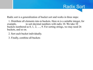
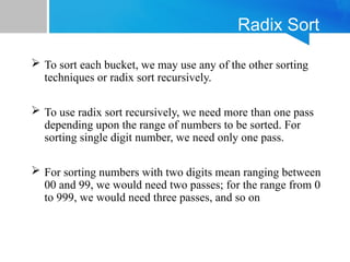
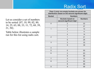
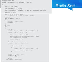
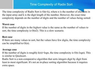

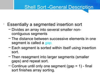
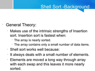
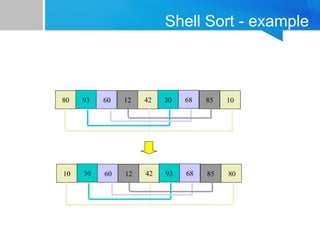
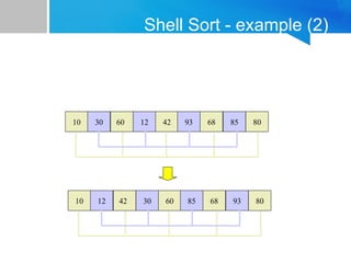

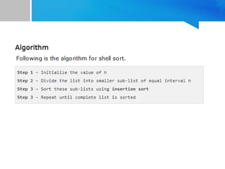
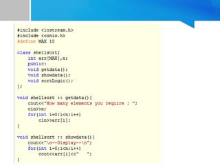

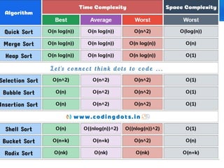

![Sequential Search
• To search the key ‘22’:
int SeqSearch(int a[], int n, key)
{
int i;
for (i=0; i<n && a[i] != key; i++)
;
if (i >= n)
return -1;
return i;
}
23
0
2
1
7
2
15
3
42
4
12
5
The search makes n key comparisons when it is unsuccessful.](https://image.slidesharecdn.com/datastructuressearchingandsorting-250503115212-17f1421f/75/Data-Structures_Searching-and-Sorting-pptx-3-2048.jpg)

![Binary Search
int BinarySearch(int a[], int n, in key)
{
int left = 0, right = n-1;
while (left <= right)
{
int middle = (left + right) / 2;
if (key < a[middle]) right = middle - 1;
else if (key > a[middle]) left = middle + 1;
else return middle;
}
return -1;
}
2
0
7
1
12
2
15
3
23
4
42
5
left right
middle
To find 23, middle
found.](https://image.slidesharecdn.com/datastructuressearchingandsorting-250503115212-17f1421f/75/Data-Structures_Searching-and-Sorting-pptx-5-2048.jpg)
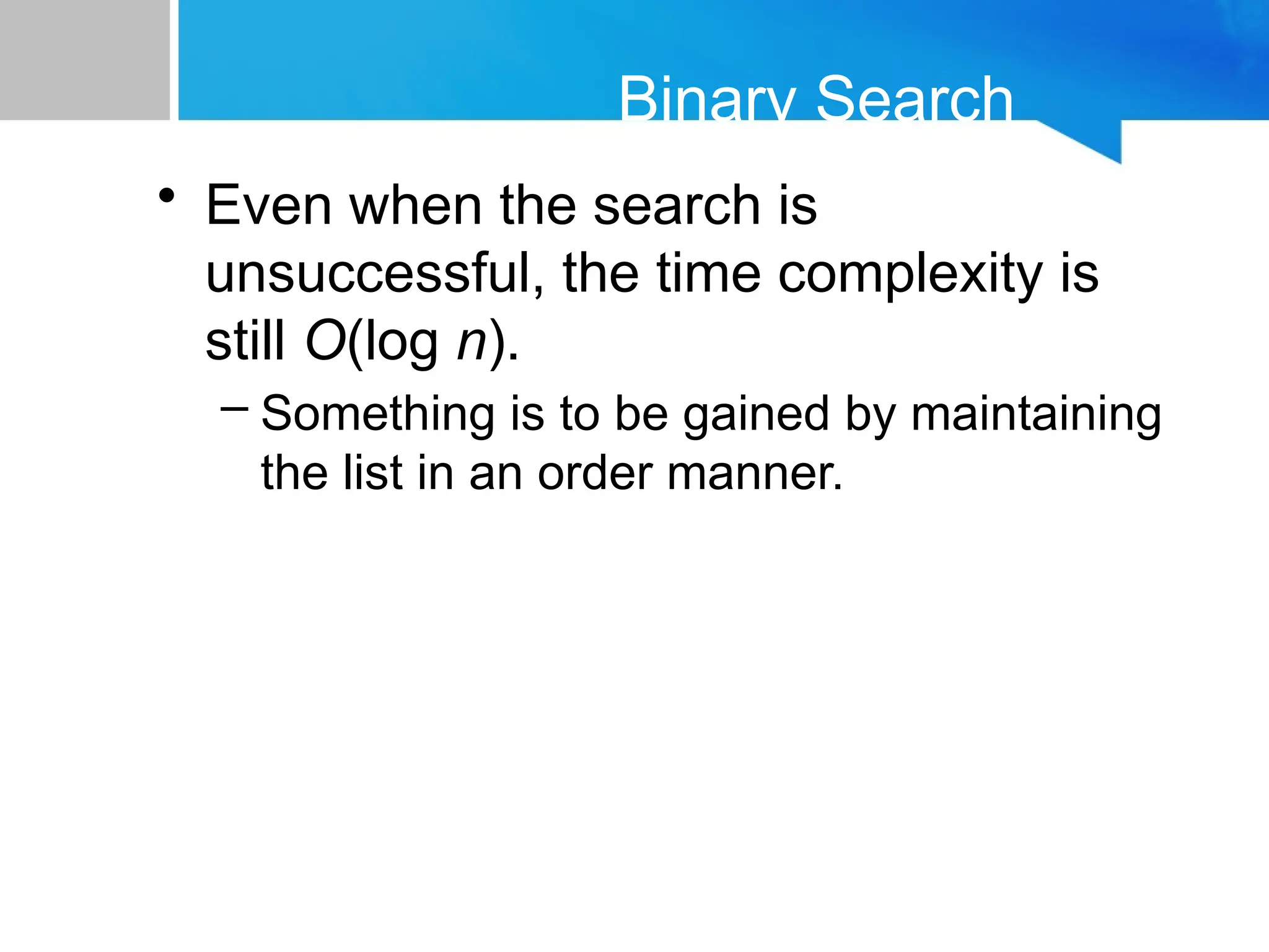
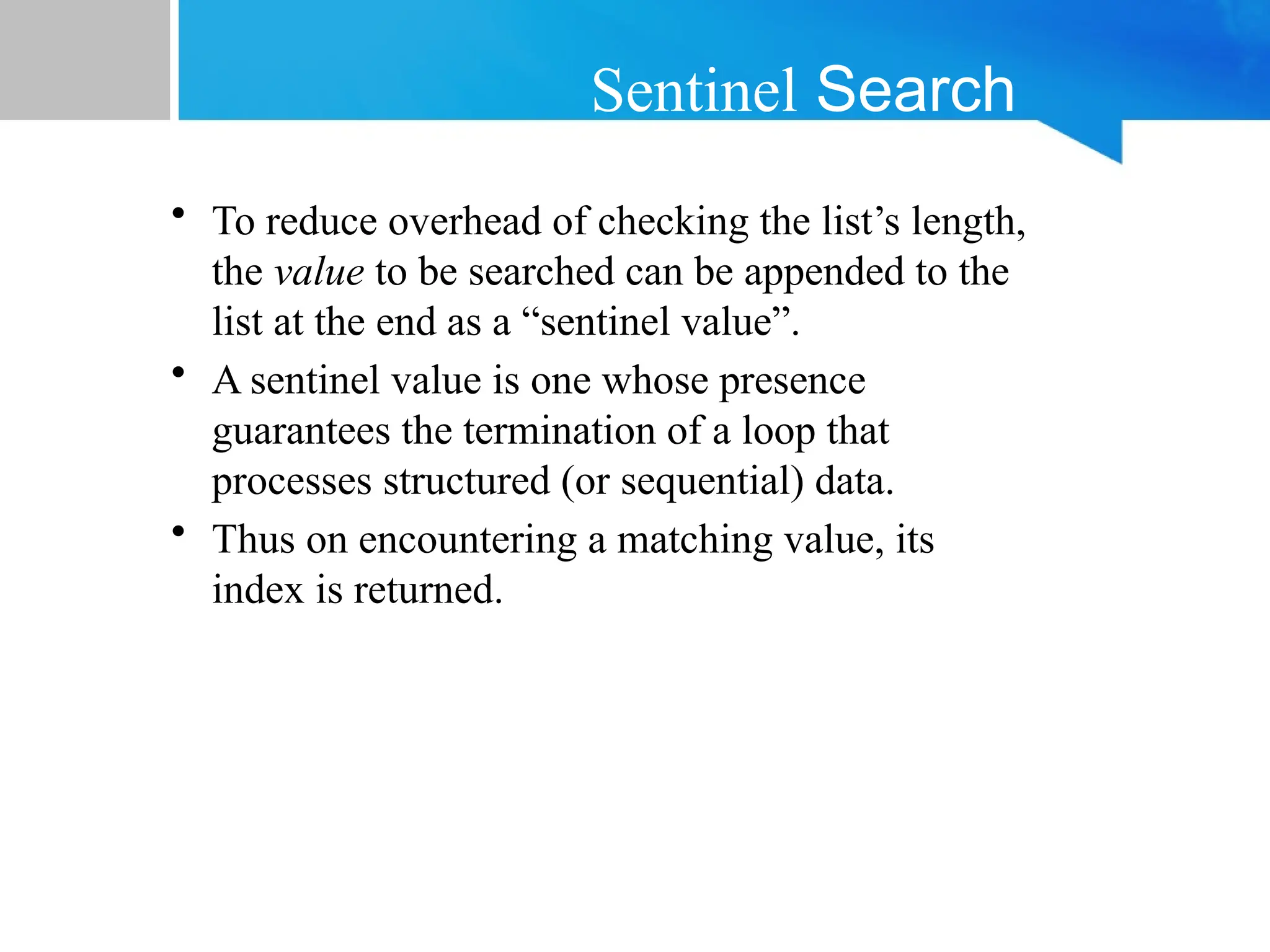
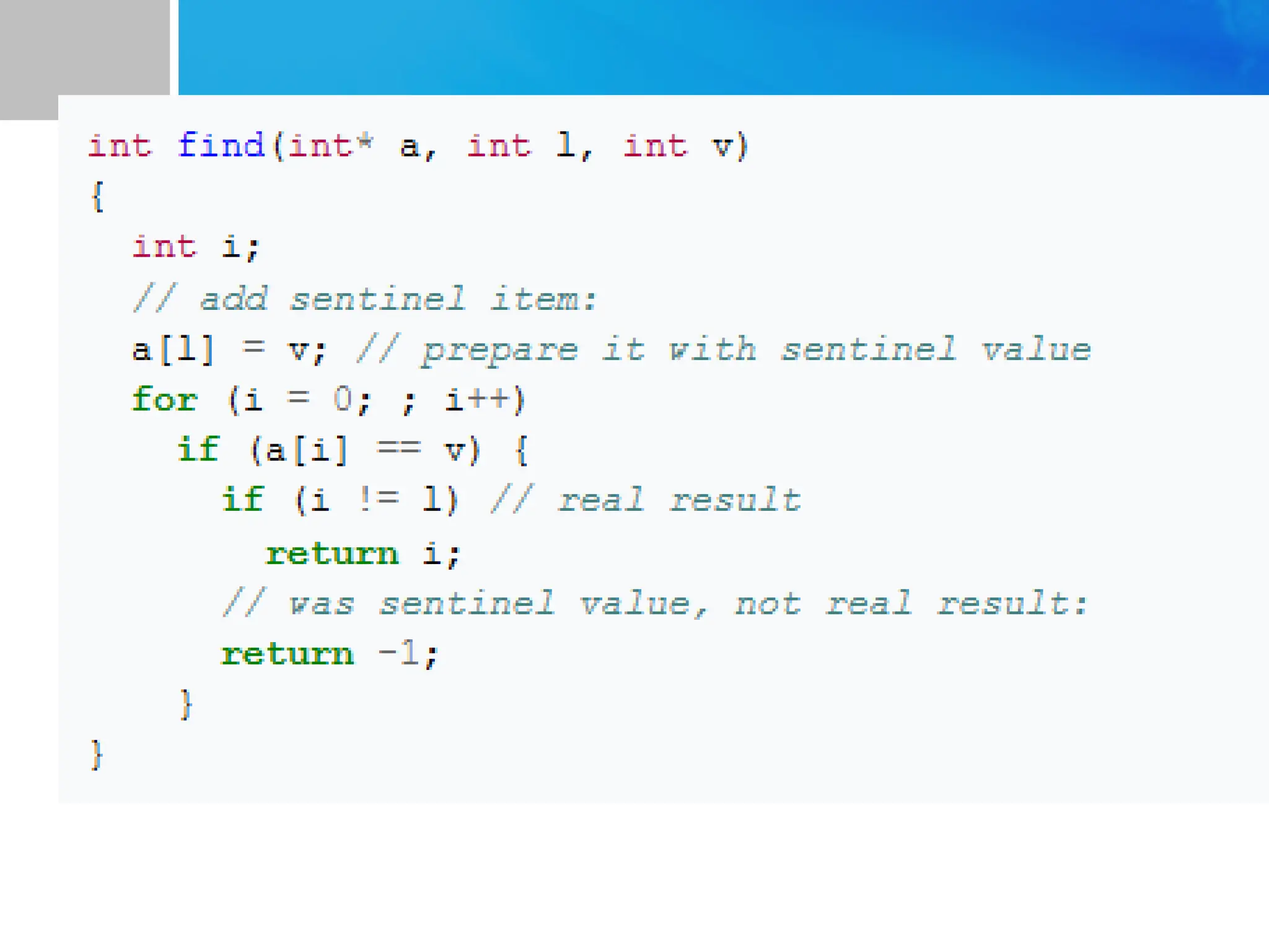

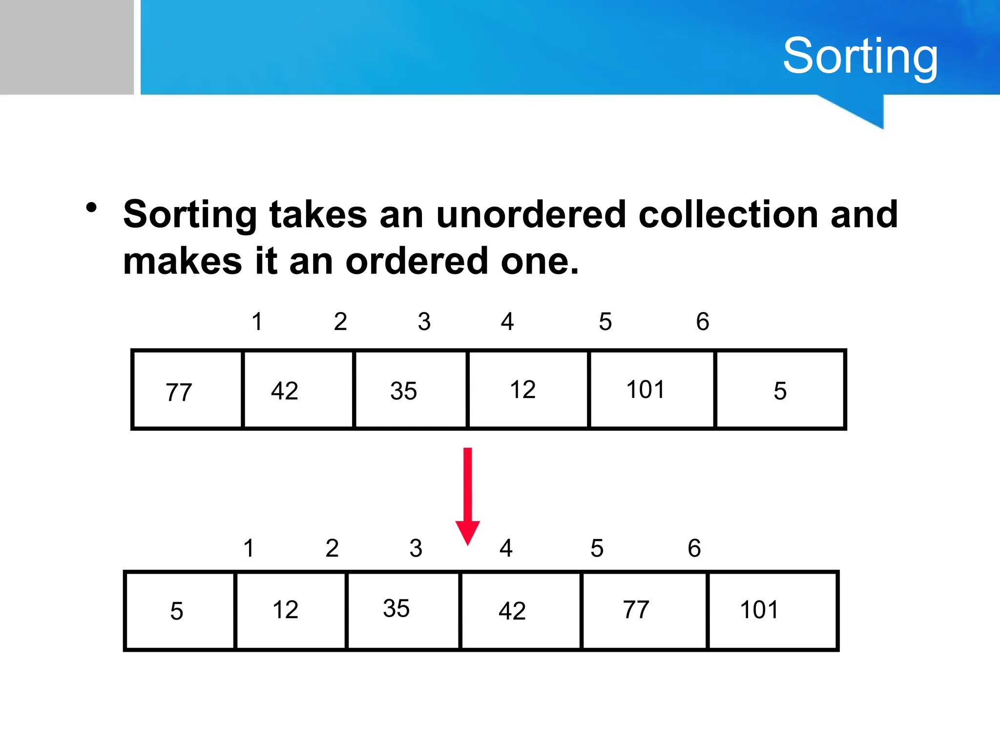
![Sorting an Array of Integers
• Example:
we are
given an
array of
six
integers
that we
want to
sort from
smallest
to largest
0
10
20
30
40
50
60
70
[1] [2] [3] [4] [5] [6]
[0] [1] [2] [3] [4] [5]](https://image.slidesharecdn.com/datastructuressearchingandsorting-250503115212-17f1421f/75/Data-Structures_Searching-and-Sorting-pptx-15-2048.jpg)


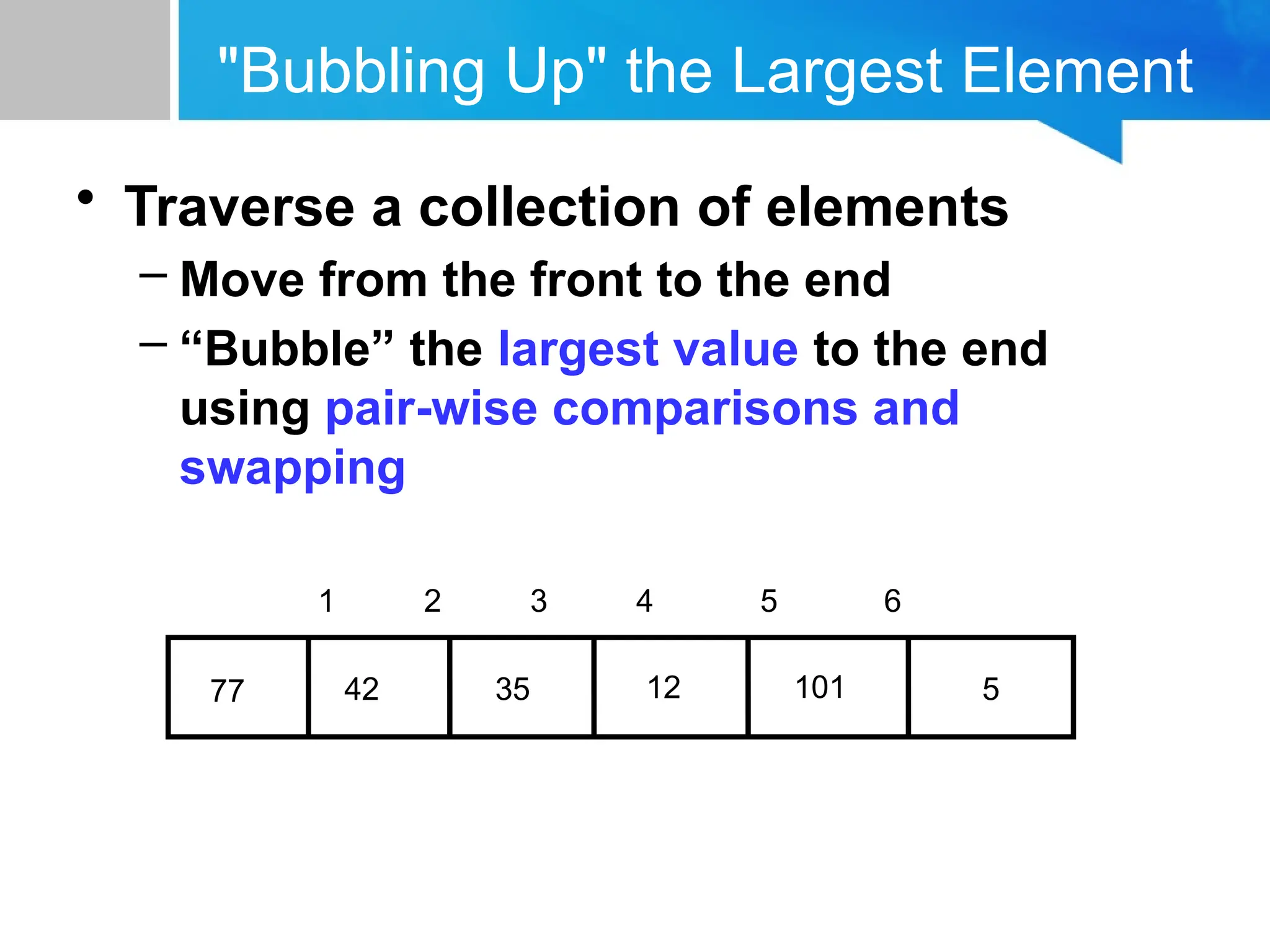
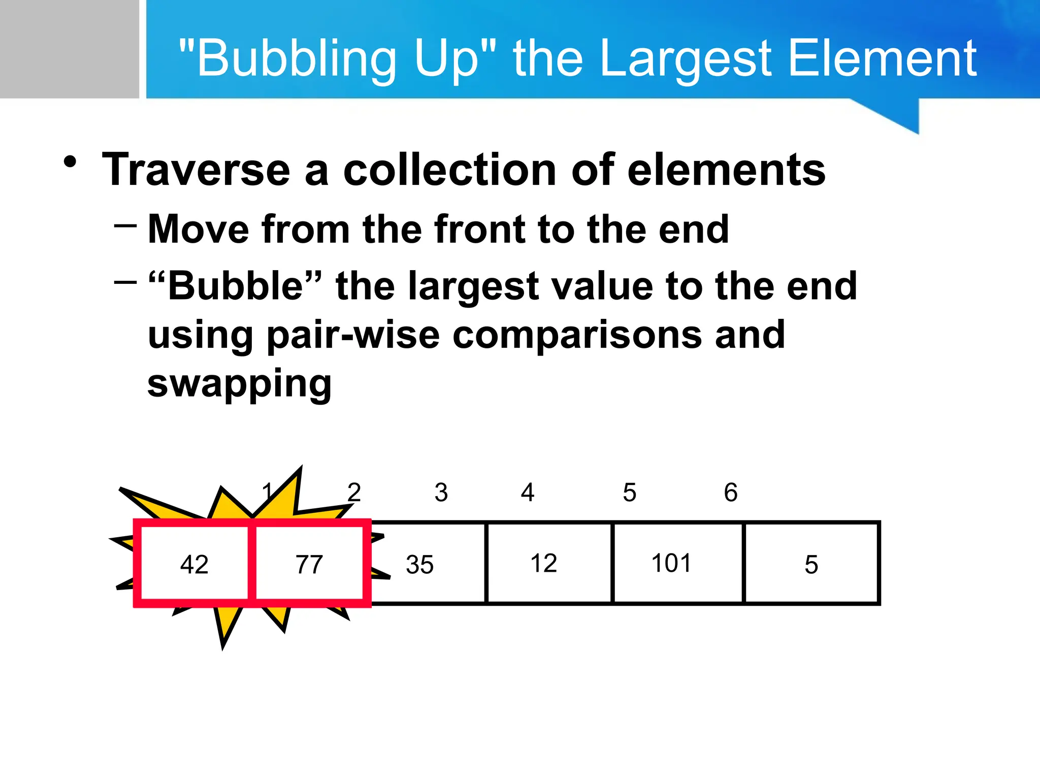

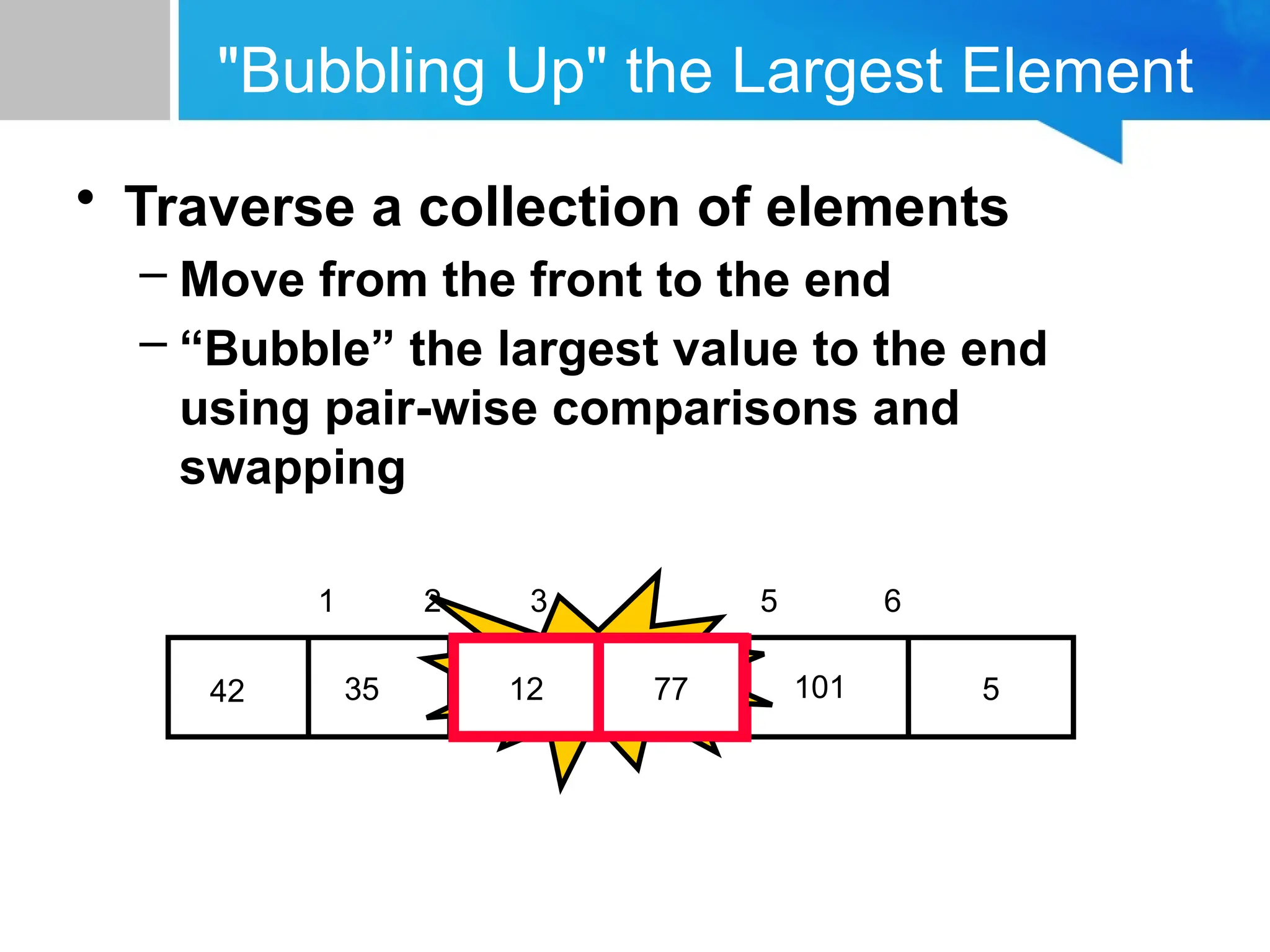

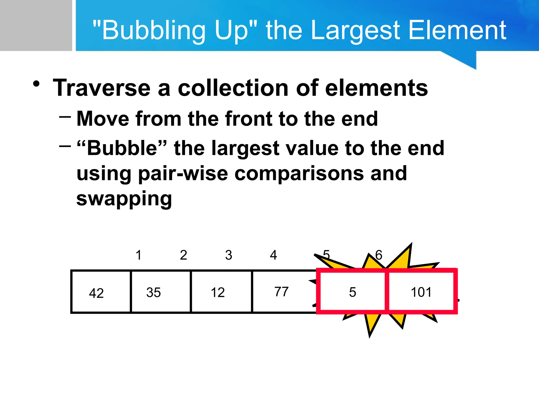
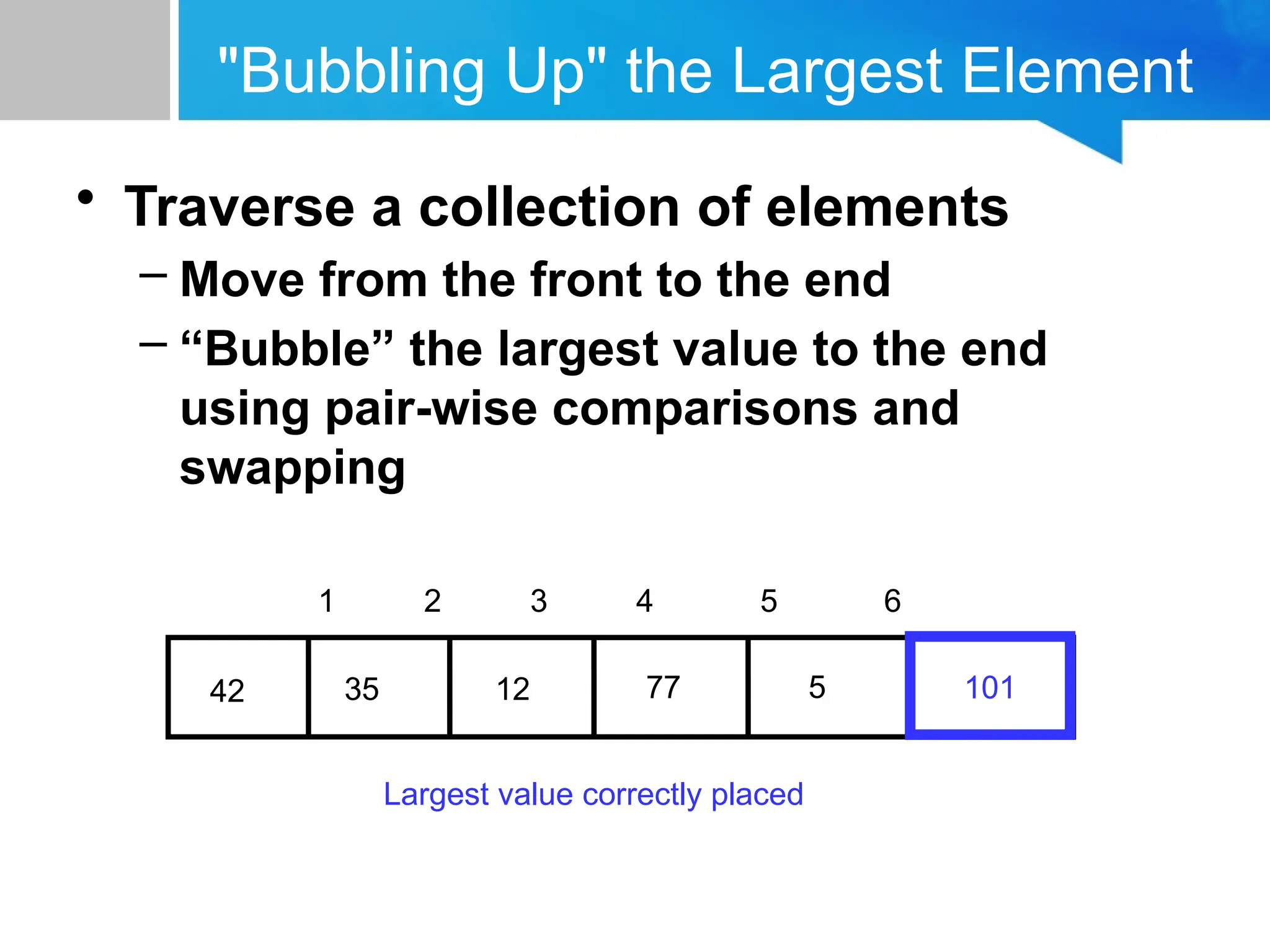
![void BubbleSort(int a[],n)
{
int i,j,temp;
for(i=1;i<n;i++)
for(j=0;j<n-i;j++)
if(a[j]>a[j+1])
{
temp=a[j];
a[j]=a[j+1];
a[j+1]=temp;
}
}](https://image.slidesharecdn.com/datastructuressearchingandsorting-250503115212-17f1421f/75/Data-Structures_Searching-and-Sorting-pptx-26-2048.jpg)
![void BubbleSort(int a[],n)
{
int i,j,temp;
for(i=1;i<n;i++)
{ bool flag = false
for(j=0;j<n-i;j++)
{ if(a[j]>a[j+1])
{ flag = true
temp=a[j];
a[j]=a[j+1];
a[j+1]=temp;
}
}
if(!flag) break;
}
}
Optimized Bubble Sort](https://image.slidesharecdn.com/datastructuressearchingandsorting-250503115212-17f1421f/75/Data-Structures_Searching-and-Sorting-pptx-27-2048.jpg)
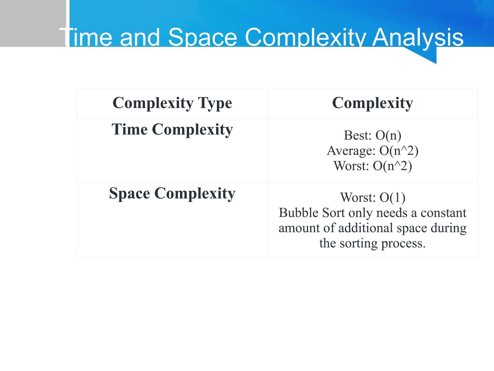

![0
10
20
30
40
50
60
70
[1] [2] [3] [4] [5] [6]
The Insertion Sort Algorithm
• The
Insertion
Sort
algorithm
also views
the array as
having a
sorted side
and an
unsorted
side.
[0] [1] [2] [3] [4] [5]](https://image.slidesharecdn.com/datastructuressearchingandsorting-250503115212-17f1421f/75/Data-Structures_Searching-and-Sorting-pptx-30-2048.jpg)
![0
10
20
30
40
50
60
70
[1] [2] [3] [4] [5] [6]
The Insertion Sort Algorithm
• The sorted
side starts
with just
the first
element,
which is
not
necessarily
the
smallest
element. 0
10
20
30
40
50
60
70
[1] [2] [3] [4] [5] [6]
[0] [1] [2] [3] [4] [5]
Sorted side Unsorted side](https://image.slidesharecdn.com/datastructuressearchingandsorting-250503115212-17f1421f/75/Data-Structures_Searching-and-Sorting-pptx-31-2048.jpg)
![0
10
20
30
40
50
60
70
[1] [2] [3] [4] [5] [6]
The Insertion Sort Algorithm
• The
sorted
side
grows by
taking the
front
element
from the
unsorted
side... 0
10
20
30
40
50
60
70
[1] [2] [3] [4] [5] [6]
[0] [1] [2] [3] [4] [5]
Sorted side Unsorted side](https://image.slidesharecdn.com/datastructuressearchingandsorting-250503115212-17f1421f/75/Data-Structures_Searching-and-Sorting-pptx-32-2048.jpg)
![0
10
20
30
40
50
60
70
[1] [2] [3] [4] [5] [6]
The Insertion Sort Algorithm
• ...and
inserting it
in the
place that
keeps the
sorted
side
arranged
from
small to
large.
0
10
20
30
40
50
60
70
[1] [2] [3] [4] [5] [6]
[0] [1] [2] [3] [4] [5]
Sorted side Unsorted side](https://image.slidesharecdn.com/datastructuressearchingandsorting-250503115212-17f1421f/75/Data-Structures_Searching-and-Sorting-pptx-33-2048.jpg)
![0
10
20
30
40
50
60
70
[1] [2] [3] [4] [5] [6]
The Insertion Sort Algorithm
0
10
20
30
40
50
60
70
[1] [2] [3] [4] [5] [6]
[0] [1] [2] [3] [4] [5]
Sorted side Unsorted side](https://image.slidesharecdn.com/datastructuressearchingandsorting-250503115212-17f1421f/75/Data-Structures_Searching-and-Sorting-pptx-34-2048.jpg)
![0
10
20
30
40
50
60
70
[1] [2] [3] [4] [5] [6]
The Insertion Sort Algorithm
• Sometime
s we are
lucky and
the new
inserted
item
doesn't
need to
move at
all.
0
10
20
30
40
50
60
70
[1] [2] [3] [4] [5] [6]
[0] [1] [2] [3] [4] [5]
Sorted side Unsorted side](https://image.slidesharecdn.com/datastructuressearchingandsorting-250503115212-17f1421f/75/Data-Structures_Searching-and-Sorting-pptx-35-2048.jpg)
![0
10
20
30
40
50
60
70
[1] [2] [3] [4] [5] [6]
The Insertionsort Algorithm
• Sometime
s we are
lucky
twice in a
row.
0
10
20
30
40
50
60
70
[1] [2] [3] [4] [5] [6]
[0] [1] [2] [3] [4] [5]
Sorted side Unsorted side](https://image.slidesharecdn.com/datastructuressearchingandsorting-250503115212-17f1421f/75/Data-Structures_Searching-and-Sorting-pptx-36-2048.jpg)
![0
10
20
30
40
50
60
70
[1] [2] [3] [4] [5] [6]
How to Insert One Element
Copy the
new
element
to a
separate
location.
0
10
20
30
40
50
60
70
[1] [2] [3] [4] [5] [6]
0
10
20
30
40
50
60
70
[1] [2] [3] [4] [5] [6]
[0] [1] [2] [3] [4] [5]
Sorted side Unsorted side](https://image.slidesharecdn.com/datastructuressearchingandsorting-250503115212-17f1421f/75/Data-Structures_Searching-and-Sorting-pptx-37-2048.jpg)
![0
10
20
30
40
50
60
70
[1] [2] [3] [4] [5] [6]
How to Insert One Element
Shift
elements
in the
sorted
side,
creating
an open
space for
the new
element.
0
10
20
30
40
50
60
70
[1] [2] [3] [4] [5] [6]
0
10
20
30
40
50
60
70
[1] [2] [3] [4] [5] [6]
[0] [1] [2] [3] [4] [5]](https://image.slidesharecdn.com/datastructuressearchingandsorting-250503115212-17f1421f/75/Data-Structures_Searching-and-Sorting-pptx-38-2048.jpg)
![0
10
20
30
40
50
60
70
[1] [2] [3] [4] [5] [6]
0
10
20
30
40
50
60
70
[1] [2] [3] [4] [5] [6]
How to Insert One Element
Shift
elements
in the
sorted
side,
creating
an open
space for
the new
element.
0
10
20
30
40
50
60
70
[1] [2] [3] [4] [5] [6]
0
10
20
30
40
50
60
70
[1] [2] [3] [4] [5] [6]
[0] [1] [2] [3] [4] [5]](https://image.slidesharecdn.com/datastructuressearchingandsorting-250503115212-17f1421f/75/Data-Structures_Searching-and-Sorting-pptx-39-2048.jpg)
![0
10
20
30
40
50
60
70
[1] [2] [3] [4] [5] [6]
0
10
20
30
40
50
60
70
[1] [2] [3] [4] [5] [6]
How to Insert One Element
Continue
shifting
elements..
.
0
10
20
30
40
50
60
70
[1] [2] [3] [4] [5] [6]
0
10
20
30
40
50
60
70
[1] [2] [3] [4] [5] [6]
[0] [1] [2] [3] [4] [5]](https://image.slidesharecdn.com/datastructuressearchingandsorting-250503115212-17f1421f/75/Data-Structures_Searching-and-Sorting-pptx-40-2048.jpg)
![0
10
20
30
40
50
60
70
[1] [2] [3] [4] [5] [6]
0
10
20
30
40
50
60
70
[1] [2] [3] [4] [5] [6]
How to Insert One Element
Continue
shifting
elements..
.
0
10
20
30
40
50
60
70
[1] [2] [3] [4] [5] [6]
0
10
20
30
40
50
60
70
[1] [2] [3] [4] [5] [6]
[0] [1] [2] [3] [4] [5]](https://image.slidesharecdn.com/datastructuressearchingandsorting-250503115212-17f1421f/75/Data-Structures_Searching-and-Sorting-pptx-41-2048.jpg)
![0
10
20
30
40
50
60
70
[1] [2] [3] [4] [5] [6]
0
10
20
30
40
50
60
70
[1] [2] [3] [4] [5] [6]
How to Insert One Element
...until you
reach the
location
for the
new
element.
0
10
20
30
40
50
60
70
[1] [2] [3] [4] [5] [6]
0
10
20
30
40
50
60
70
[1] [2] [3] [4] [5] [6]
[0] [1] [2] [3] [4] [5]](https://image.slidesharecdn.com/datastructuressearchingandsorting-250503115212-17f1421f/75/Data-Structures_Searching-and-Sorting-pptx-42-2048.jpg)
![0
10
20
30
40
50
60
70
[1] [2] [3] [4] [5] [6]
0
10
20
30
40
50
60
70
[1] [2] [3] [4] [5] [6]
How to Insert One Element
Copy the
new
element
back into
the array,
at the
correct
location.
0
10
20
30
40
50
60
70
[1] [2] [3] [4] [5] [6]
[0] [1] [2] [3] [4] [5]
Sorted side Unsorted side](https://image.slidesharecdn.com/datastructuressearchingandsorting-250503115212-17f1421f/75/Data-Structures_Searching-and-Sorting-pptx-43-2048.jpg)
![0
10
20
30
40
50
60
70
[1] [2] [3] [4] [5] [6]
How to Insert One Element
0
10
20
30
40
50
60
70
[1] [2] [3] [4] [5] [6]
• The last
element
must also
be
inserted.
Start by
copying
it...
[0] [1] [2] [3] [4] [5]
Sorted side Unsorted side](https://image.slidesharecdn.com/datastructuressearchingandsorting-250503115212-17f1421f/75/Data-Structures_Searching-and-Sorting-pptx-44-2048.jpg)
![0
10
20
30
40
50
60
70
[1] [2] [3] [4] [5] [6]
Sorted Result
[0] [1] [2] [3] [4] [5]](https://image.slidesharecdn.com/datastructuressearchingandsorting-250503115212-17f1421f/75/Data-Structures_Searching-and-Sorting-pptx-45-2048.jpg)
![void insertion_sort (int data[], int n)
{
int i, j;
int temp;
if(n < 2) return; // nothing to sort!!
for(i = 1; i < n; ++i)
{
// take next item at front of unsorted part of array
// and insert it in appropriate location in sorted part of array
temp = data[i];
for(j = i; data[j-1] > temp && j > 0; --j)
data[j] = data[j-1]; // shift element forward
data[j] = temp;
}
}](https://image.slidesharecdn.com/datastructuressearchingandsorting-250503115212-17f1421f/75/Data-Structures_Searching-and-Sorting-pptx-46-2048.jpg)
![Insertion Sort Time Analysis
• In O-notation, what is:
– Worst case running time for n items?
– Average case running time for n items?
• Steps of algorithm:
for i = 1 to n-1
take next key from unsorted part of array
insert in appropriate location in sorted part of array:
for j = i down to 0,
shift sorted elements to the right if key > key[i]
increase size of sorted array by 1
Outer loop:
O(n)](https://image.slidesharecdn.com/datastructuressearchingandsorting-250503115212-17f1421f/75/Data-Structures_Searching-and-Sorting-pptx-47-2048.jpg)
![Insertion Sort Time Analysis
• In O-notation, what is:
– Worst case running time for n items?
– Average case running time for n items?
• Steps of algorithm:
for i = 1 to n-1
take next key from unsorted part of array
insert in appropriate location in sorted part of array:
for j = i down to 0,
shift sorted elements to the right if key > key[i]
increase size of sorted array by 1
Outer loop:
O(n)
Inner loop:
O(n)](https://image.slidesharecdn.com/datastructuressearchingandsorting-250503115212-17f1421f/75/Data-Structures_Searching-and-Sorting-pptx-48-2048.jpg)
![template <class Item>
void insertion_sort(Item data[ ], size_t n)
{
size_t i, j;
Item temp;
if(n < 2) return; // nothing to sort!!
for(i = 1; i < n; ++i)
{
// take next item at front of unsorted part of array
// and insert it in appropriate location in sorted part of array
temp = data[i];
for(j = i; data[j-1] > temp and j > 0; --j)
data[j] = data[j-1]; // shift element forward
data[j] = temp;
}
}
O(n)
O(n)](https://image.slidesharecdn.com/datastructuressearchingandsorting-250503115212-17f1421f/75/Data-Structures_Searching-and-Sorting-pptx-49-2048.jpg)
![Insertion Sort Time Analysis
• Steps of algorithm:
for i = 1 to n-1
take next key from unsorted part of array
insert in appropriate location in sorted part of array:
for j = i down to 0,
shift sorted elements to the right if key > key[i]
increase size of sorted array by 1](https://image.slidesharecdn.com/datastructuressearchingandsorting-250503115212-17f1421f/75/Data-Structures_Searching-and-Sorting-pptx-50-2048.jpg)

![0
10
20
30
40
50
60
70
[1] [2] [3] [4] [5] [6]
The Selection Sort Algorithm
• Start by
finding the
smallest
entry.
0
10
20
30
40
50
60
70
[1] [2] [3] [4] [5] [6]
[0] [1] [2] [3] [4] [5]](https://image.slidesharecdn.com/datastructuressearchingandsorting-250503115212-17f1421f/75/Data-Structures_Searching-and-Sorting-pptx-53-2048.jpg)
![0
10
20
30
40
50
60
70
[1] [2] [3] [4] [5] [6]
The Selection Sort Algorithm
• Swap the
smallest
entry with
the first
entry.
0
10
20
30
40
50
60
70
[1] [2] [3] [4] [5] [6]
[0] [1] [2] [3] [4] [5]](https://image.slidesharecdn.com/datastructuressearchingandsorting-250503115212-17f1421f/75/Data-Structures_Searching-and-Sorting-pptx-54-2048.jpg)
![0
10
20
30
40
50
60
70
[1] [2] [3] [4] [5] [6]
The Selection Sort Algorithm
• Swap the
smallest
entry with
the first
entry.
0
10
20
30
40
50
60
70
[1] [2] [3] [4] [5] [6]
[0] [1] [2] [3] [4] [5]](https://image.slidesharecdn.com/datastructuressearchingandsorting-250503115212-17f1421f/75/Data-Structures_Searching-and-Sorting-pptx-55-2048.jpg)
![0
10
20
30
40
50
60
70
[1] [2] [3] [4] [5] [6]
The Selection Sort Algorithm
• Part of the
array is
now
sorted.
0
10
20
30
40
50
60
70
[1] [2] [3] [4] [5] [6]
Sorted side Unsorted side
[0] [1] [2] [3] [4] [5]](https://image.slidesharecdn.com/datastructuressearchingandsorting-250503115212-17f1421f/75/Data-Structures_Searching-and-Sorting-pptx-56-2048.jpg)
![0
10
20
30
40
50
60
70
[1] [2] [3] [4] [5] [6]
0
10
20
30
40
50
60
70
[1] [2] [3] [4] [5] [6]
The Selection Sort Algorithm
• Find the
smallest
element in
the
unsorted
side.
Sorted side Unsorted side
[0] [1] [2] [3] [4] [5]](https://image.slidesharecdn.com/datastructuressearchingandsorting-250503115212-17f1421f/75/Data-Structures_Searching-and-Sorting-pptx-57-2048.jpg)
![0
10
20
30
40
50
60
70
[1] [2] [3] [4] [5] [6]
0
10
20
30
40
50
60
70
[1] [2] [3] [4] [5] [6]
The Selection Sort Algorithm
• Swap with
the front
of the
unsorted
side.
Sorted side Unsorted side
[0] [1] [2] [3] [4] [5]](https://image.slidesharecdn.com/datastructuressearchingandsorting-250503115212-17f1421f/75/Data-Structures_Searching-and-Sorting-pptx-58-2048.jpg)
![0
10
20
30
40
50
60
70
[1] [2] [3] [4] [5] [6]
0
10
20
30
40
50
60
70
[1] [2] [3] [4] [5] [6]
The Selection Sort Algorithm
• We have
increased
the size of
the sorted
side by
one
element.
Sorted side Unsorted side
[0] [1] [2] [3] [4] [5]](https://image.slidesharecdn.com/datastructuressearchingandsorting-250503115212-17f1421f/75/Data-Structures_Searching-and-Sorting-pptx-59-2048.jpg)
![0
10
20
30
40
50
60
70
[1] [2] [3] [4] [5] [6]
0
10
20
30
40
50
60
70
[1] [2] [3] [4] [5] [6]
The Selection Sort Algorithm
• The
process
continues.
..
Sorted side Unsorted side
Smallest
from
unsorted
[0] [1] [2] [3] [4] [5]](https://image.slidesharecdn.com/datastructuressearchingandsorting-250503115212-17f1421f/75/Data-Structures_Searching-and-Sorting-pptx-60-2048.jpg)
![0
10
20
30
40
50
60
70
[1] [2] [3] [4] [5] [6]
0
10
20
30
40
50
60
70
[1] [2] [3] [4] [5] [6]
The Selection Sort Algorithm
• The
process
continues.
..
Sorted side Unsorted side
[0] [1] [2] [3] [4] [5]
Swap
with
front](https://image.slidesharecdn.com/datastructuressearchingandsorting-250503115212-17f1421f/75/Data-Structures_Searching-and-Sorting-pptx-61-2048.jpg)
![0
10
20
30
40
50
60
70
[1] [2] [3] [4] [5] [6]
0
10
20
30
40
50
60
70
[1] [2] [3] [4] [5] [6]
The Selection Sort Algorithm
• The
process
continues.
..
Sorted side Unsorted side
Sorted side
is bigger
[0] [1] [2] [3] [4] [5]](https://image.slidesharecdn.com/datastructuressearchingandsorting-250503115212-17f1421f/75/Data-Structures_Searching-and-Sorting-pptx-62-2048.jpg)
![0
10
20
30
40
50
60
70
[1] [2] [3] [4] [5] [6]
0
10
20
30
40
50
60
70
[1] [2] [3] [4] [5] [6]
The Selection Sort Algorithm
• The process
keeps adding
one more
number to the
sorted side.
• The sorted
side has the
smallest
numbers,
arranged from
small to large.
Sorted side Unsorted side
[0] [1] [2] [3] [4] [5]](https://image.slidesharecdn.com/datastructuressearchingandsorting-250503115212-17f1421f/75/Data-Structures_Searching-and-Sorting-pptx-63-2048.jpg)
![0
10
20
30
40
50
60
70
[1] [2] [3] [4] [5] [6]
0
10
20
30
40
50
60
70
[1] [2] [3] [4] [5] [6]
The Selection Sort Algorithm
• We can stop
when the
unsorted
side has just
one number,
since that
number must
be the
largest
number.
[0] [1] [2] [3] [4] [5]
Sorted side Unsorted side](https://image.slidesharecdn.com/datastructuressearchingandsorting-250503115212-17f1421f/75/Data-Structures_Searching-and-Sorting-pptx-64-2048.jpg)
![0
10
20
30
40
50
60
70
[1] [2] [3] [4] [5] [6]
The Selection Sort Algorithm
• The array is
now sorted.
• We
repeatedly
selected the
smallest
element, and
moved this
element to
the front of
the unsorted [0] [1] [2] [3] [4] [5]](https://image.slidesharecdn.com/datastructuressearchingandsorting-250503115212-17f1421f/75/Data-Structures_Searching-and-Sorting-pptx-65-2048.jpg)
![void selectionsort(int arr[], int n)
{
int i, j, min_idx;
// One by one move boundary of
// unsorted subarray
for (i = 0; i < n-1; i++)
{
// Find the minimum element in
// unsorted array
min_idx = i;
for (j = i+1; j < n; j++)
if (arr[j] < arr[min_idx])
min_idx = j;
// Swap the found minimum element
// with the first element
int temp = arr[min_idx];
arr[min_idx] = arr[i];
arr[i] = temp;
} }](https://image.slidesharecdn.com/datastructuressearchingandsorting-250503115212-17f1421f/75/Data-Structures_Searching-and-Sorting-pptx-66-2048.jpg)
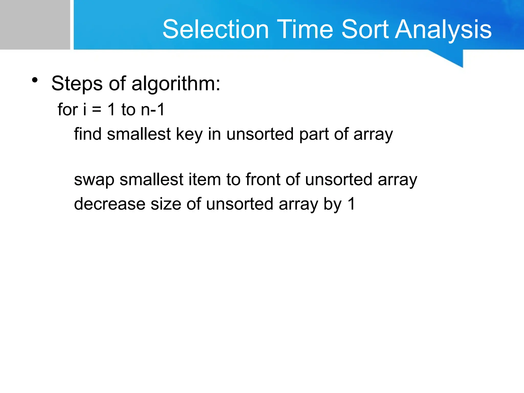
![template <class Item>
void selection_sort(Item data[ ], size_t n)
{
size_t i, j, smallest;
Item temp;
if(n < 2) return; // nothing to sort!!
for(i = 0; i < n-1 ; ++i)
{
// find smallest in unsorted part of array
smallest = i;
for(j = i+1; j < n; ++j)
if(data[smallest] > data[j]) smallest = j;
// put it at front of unsorted part of array (swap)
temp = data[i];
data[i] = data[smallest];
data[smallest] = temp;
}
}
Outer loop:
O(n)](https://image.slidesharecdn.com/datastructuressearchingandsorting-250503115212-17f1421f/75/Data-Structures_Searching-and-Sorting-pptx-68-2048.jpg)
![template <class Item>
void selection_sort(Item data[ ], size_t n)
{
size_t i, j, smallest;
Item temp;
if(n < 2) return; // nothing to sort!!
for(i = 0; i < n-1 ; ++i)
{
// find smallest in unsorted part of array
smallest = i;
for(j = i+1; j < n; ++j)
if(data[smallest] > data[j]) smallest = j;
// put it at front of unsorted part of array (swap)
temp = data[i];
data[i] = data[smallest];
data[smallest] = temp;
}
}
Outer loop:
O(n)
Inner loop:
O(n)](https://image.slidesharecdn.com/datastructuressearchingandsorting-250503115212-17f1421f/75/Data-Structures_Searching-and-Sorting-pptx-69-2048.jpg)
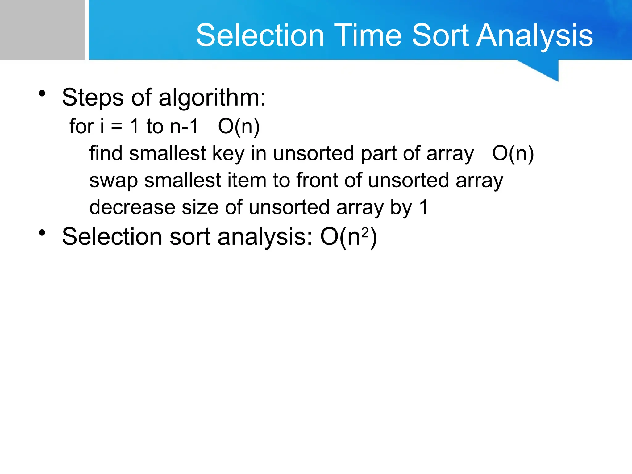
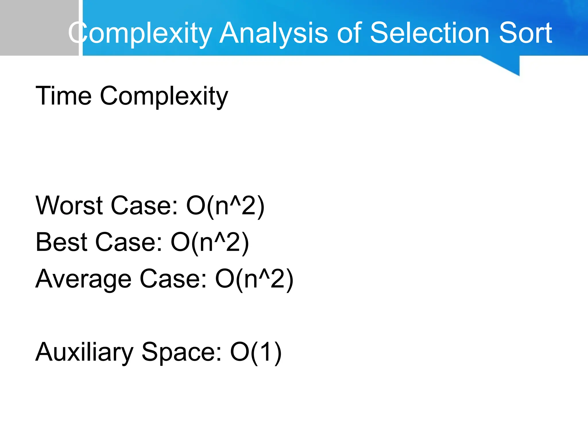
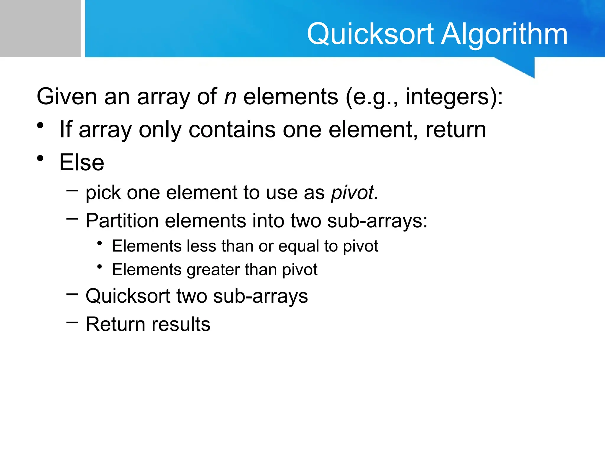

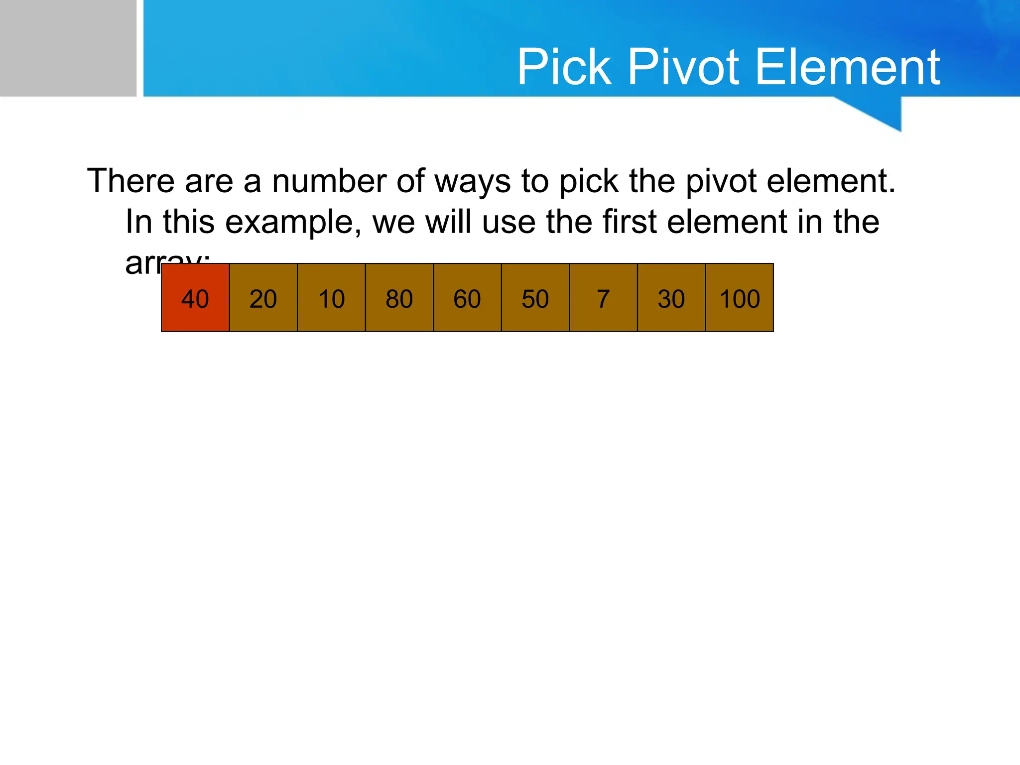

![40 20 10 80 60 50 7 30 100
pivot_index = 0
[0] [1] [2] [3] [4] [5] [6] [7] [8]
i j](https://image.slidesharecdn.com/datastructuressearchingandsorting-250503115212-17f1421f/75/Data-Structures_Searching-and-Sorting-pptx-76-2048.jpg)
![40 20 10 80 60 50 7 30 100
pivot_index = 0
[0] [1] [2] [3] [4] [5] [6] [7] [8]
1. While data[i] <= data[pivot]
++i
i j](https://image.slidesharecdn.com/datastructuressearchingandsorting-250503115212-17f1421f/75/Data-Structures_Searching-and-Sorting-pptx-77-2048.jpg)
![40 20 10 80 60 50 7 30 100
pivot_index = 0
[0] [1] [2] [3] [4] [5] [6] [7] [8]
1. While data[i] <= data[pivot]
++i
i j](https://image.slidesharecdn.com/datastructuressearchingandsorting-250503115212-17f1421f/75/Data-Structures_Searching-and-Sorting-pptx-78-2048.jpg)
![40 20 10 80 60 50 7 30 100
pivot_index = 0
[0] [1] [2] [3] [4] [5] [6] [7] [8]
1. While data[i] <= data[pivot]
++i
j
i](https://image.slidesharecdn.com/datastructuressearchingandsorting-250503115212-17f1421f/75/Data-Structures_Searching-and-Sorting-pptx-79-2048.jpg)
![40 20 10 80 60 50 7 30 100
pivot_index = 0
[0] [1] [2] [3] [4] [5] [6] [7] [8]
j
1. While data[i] <= data[pivot]
++i
2. While data[j] > data[pivot]
--j
i](https://image.slidesharecdn.com/datastructuressearchingandsorting-250503115212-17f1421f/75/Data-Structures_Searching-and-Sorting-pptx-80-2048.jpg)
![40 20 10 80 60 50 7 30 100
pivot_index = 0
[0] [1] [2] [3] [4] [5] [6] [7] [8]
i j
1. While data[i] <= data[pivot]
++
2. While data[j] > data[pivot]
--j](https://image.slidesharecdn.com/datastructuressearchingandsorting-250503115212-17f1421f/75/Data-Structures_Searching-and-Sorting-pptx-81-2048.jpg)
![40 20 10 80 60 50 7 30 100
pivot_index = 0
[0] [1] [2] [3] [4] [5] [6] [7] [8]
i j
1. While data[i] <= data[pivot]
++i
2. While data[j] > data[pivot]
--j
3. If i < j
swap data[i] and data[j]](https://image.slidesharecdn.com/datastructuressearchingandsorting-250503115212-17f1421f/75/Data-Structures_Searching-and-Sorting-pptx-82-2048.jpg)
![40 20 10 30 60 50 7 80 100
pivot_index = 0
[0] [1] [2] [3] [4] [5] [6] [7] [8]
i j
1. While data[i] <= data[pivot]
++i
2. While data[j] > data[pivot]
--j
3. If i< j
swap data[i] and data[j]](https://image.slidesharecdn.com/datastructuressearchingandsorting-250503115212-17f1421f/75/Data-Structures_Searching-and-Sorting-pptx-83-2048.jpg)
![40 20 10 30 60 50 7 80 100
pivot_index = 0
[0] [1] [2] [3] [4] [ 5] [6] [7] [8]
i j
1. While data[i] <= data[pivot]
++i
2. While data[j] > data[pivot]
--j
3. If i < j
swap data[i] and data[j]
4. While j > i go to 1.](https://image.slidesharecdn.com/datastructuressearchingandsorting-250503115212-17f1421f/75/Data-Structures_Searching-and-Sorting-pptx-84-2048.jpg)
![40 20 10 30 60 50 7 80 100
pivot_index = 0
[0] [1] [2] [3] [4] [5] [6] [7] [8]
i j
1. While data[i] <= data[pivot]
++i
2. While data[j] > data[pivot]
--j
3. If i<j
swap data[i] and data[j]
4. While j> i, go to 1.](https://image.slidesharecdn.com/datastructuressearchingandsorting-250503115212-17f1421f/75/Data-Structures_Searching-and-Sorting-pptx-85-2048.jpg)
![40 20 10 30 60 50 7 80 100
pivot_index = 0
[0] [1] [2] [3] [4] [5] [6] [7] [8]
i j
1. While data[i] <= data[pivot]
++i
2. While data[j] > data[pivot]
--j
3. If i< j
swap data[i] and data[j]
4. While j > i, go to 1.](https://image.slidesharecdn.com/datastructuressearchingandsorting-250503115212-17f1421f/75/Data-Structures_Searching-and-Sorting-pptx-86-2048.jpg)
![40 20 10 30 60 50 7 80 100
pivot_index = 0
[0] [1] [2] [3] [4] [5] [6] [7] [8]
i j
1. While data[i] <= data[pivot]
++i
2. While data[j] > data[pivot]
--j
3. If i < j
swap data[i] and data[j]
4. While j > i, go to 1.](https://image.slidesharecdn.com/datastructuressearchingandsorting-250503115212-17f1421f/75/Data-Structures_Searching-and-Sorting-pptx-87-2048.jpg)
![40 20 10 30 60 50 7 80 100
pivot_index = 0
[0] [1] [2] [3] [4] [5] [6] [7] [8]
i j
1. While data[i] <= data[pivot]
++i
2. While data[j] > data[pivot]
--j
3. If i < j
swap data[i] and data[j]
4. While j > i, go to 1.](https://image.slidesharecdn.com/datastructuressearchingandsorting-250503115212-17f1421f/75/Data-Structures_Searching-and-Sorting-pptx-88-2048.jpg)
![40 20 10 30 60 50 7 80 100
pivot_index = 0
[0] [1] [2] [3] [4] [5] [6] [7] [8]
i j
1. While data[i] <= data[pivot]
++i
2. While data[j] > data[pivot]
--j
3. If i < j
swap data[i] and data[j]
4. While j> i, go to 1.](https://image.slidesharecdn.com/datastructuressearchingandsorting-250503115212-17f1421f/75/Data-Structures_Searching-and-Sorting-pptx-89-2048.jpg)
![1. While data[i] <= data[pivot]
++i
2. While data[j] > data[pivot]
--j
3. If i < j
swap data[i] and data[j]
4. While j> i, go to 1.
40 20 10 30 7 50 60 80 100
pivot_index = 0
[0] [1] [2] [3] [4] [5] [6] [7] [8]
i j](https://image.slidesharecdn.com/datastructuressearchingandsorting-250503115212-17f1421f/75/Data-Structures_Searching-and-Sorting-pptx-90-2048.jpg)
![1. While data[i] <= data[pivot]
++i
2. While data[j] > data[pivot]
--j
3. If i< j
swap data[i] and data[j]
4. While j> i, go to 1.
40 20 10 30 7 50 60 80 100
pivot_index = 0
[0] [1] [2] [3] [4] [5] [6] [7] [8]
i j](https://image.slidesharecdn.com/datastructuressearchingandsorting-250503115212-17f1421f/75/Data-Structures_Searching-and-Sorting-pptx-91-2048.jpg)
![1. While data[i] <= data[pivot]
++i
2. While data[j] > data[pivot]
--j
3. If i < j
swap data[i] and data[j]
4. While j > i, go to 1.
40 20 10 30 7 50 60 80 100
pivot_index = 0
[0] [1] [2] [3] [4] [5] [6] [7] [8]
i j](https://image.slidesharecdn.com/datastructuressearchingandsorting-250503115212-17f1421f/75/Data-Structures_Searching-and-Sorting-pptx-92-2048.jpg)
![1. While data[i] <= data[pivot]
++i
2. While data[j] > data[pivot]
--j
3. If i < j
swap data[i] and data[j]
4. While j > i, go to 1.
40 20 10 30 7 50 60 80 100
pivot_index = 0
[0] [1] [2] [3] [4] [5] [6] [7] [8]
i j](https://image.slidesharecdn.com/datastructuressearchingandsorting-250503115212-17f1421f/75/Data-Structures_Searching-and-Sorting-pptx-93-2048.jpg)
![1. While data[i] <= data[pivot]
++i
2. While data[j] > data[pivot]
--j
3. If i< j
swap data[i] and data[j]
4. While j > i, go to 1.
40 20 10 30 7 50 60 80 100
pivot_index = 0
[0] [1] [2] [3] [4] [5] [6] [7] [8]
i j](https://image.slidesharecdn.com/datastructuressearchingandsorting-250503115212-17f1421f/75/Data-Structures_Searching-and-Sorting-pptx-94-2048.jpg)
![1. While data[i] <= data[pivot]
++i
2. While data[j] > data[pivot]
--j
3. If i < j
swap data[i] and data[j]
4. While j > i, go to 1.
40 20 10 30 7 50 60 80 100
pivot_index = 0
[0] [1] [2] [3] [4] [5] [6] [7] [8]
i j](https://image.slidesharecdn.com/datastructuressearchingandsorting-250503115212-17f1421f/75/Data-Structures_Searching-and-Sorting-pptx-95-2048.jpg)
![1. While data[i] <= data[pivot]
++i
2. While data[j] > data[pivot]
--j
3. If i < j
swap data[i] and data[j]
4. While j > i, go to 1.
40 20 10 30 7 50 60 80 100
pivot_index = 0
[0] [1] [2] [3] [4] [5] [6] [7] [8]
i j](https://image.slidesharecdn.com/datastructuressearchingandsorting-250503115212-17f1421f/75/Data-Structures_Searching-and-Sorting-pptx-96-2048.jpg)
![1. While data[i] <= data[pivot]
++i
2. While data[j] > data[pivot]
--j
3. If i < j
swap data[i] and data[j]
4. While j > i, go to 1.
40 20 10 30 7 50 60 80 100
pivot_index = 0
[0] [1] [2] [3] [4] [5] [6] [7] [8]
i j](https://image.slidesharecdn.com/datastructuressearchingandsorting-250503115212-17f1421f/75/Data-Structures_Searching-and-Sorting-pptx-97-2048.jpg)
![1. While data[i] <= data[pivot]
++i
2. While data[j] > data[pivot]
--j
3. If i<j
swap data[i] and data[j]
4. While j > i, go to 1.
40 20 10 30 7 50 60 80 100
pivot_index = 0
[0] [1] [2] [3] [4] [5] [6] [7] [8]
i j](https://image.slidesharecdn.com/datastructuressearchingandsorting-250503115212-17f1421f/75/Data-Structures_Searching-and-Sorting-pptx-98-2048.jpg)
![1. While data[i] <= data[pivot]
++I
2. While data[j] > data[pivot]
--j
3. If i < j
swap data[i] and data[j]
4. While j > i, go to 1.
5. Swap data[j] and data[pivot_index]
40 20 10 30 7 50 60 80 100
pivot_index = 0
[0] [1] [2] [3] [4] [5] [6] [7] [8]
i j](https://image.slidesharecdn.com/datastructuressearchingandsorting-250503115212-17f1421f/75/Data-Structures_Searching-and-Sorting-pptx-99-2048.jpg)
![1. While data[i] <= data[pivot]
++I
2. While data[j] > data[pivot]
--j
3. If i<j
swap data[i] and data[j]
4. While j > i, go to 1.
5. Swap data[j] and
data[pivot_index]
7 20 10 30 40 50 60 80 100
pivot_index = 4
[0] [1] [2] [3] [4] [5] [6] [7] [8]
i j](https://image.slidesharecdn.com/datastructuressearchingandsorting-250503115212-17f1421f/75/Data-Structures_Searching-and-Sorting-pptx-100-2048.jpg)
![Partition Result
7 20 10 30 40 50 60 80 100
[0] [1] [2] [3] [4] [5] [6] [7] [8]
<= data[pivot] > data[pivot]](https://image.slidesharecdn.com/datastructuressearchingandsorting-250503115212-17f1421f/75/Data-Structures_Searching-and-Sorting-pptx-101-2048.jpg)
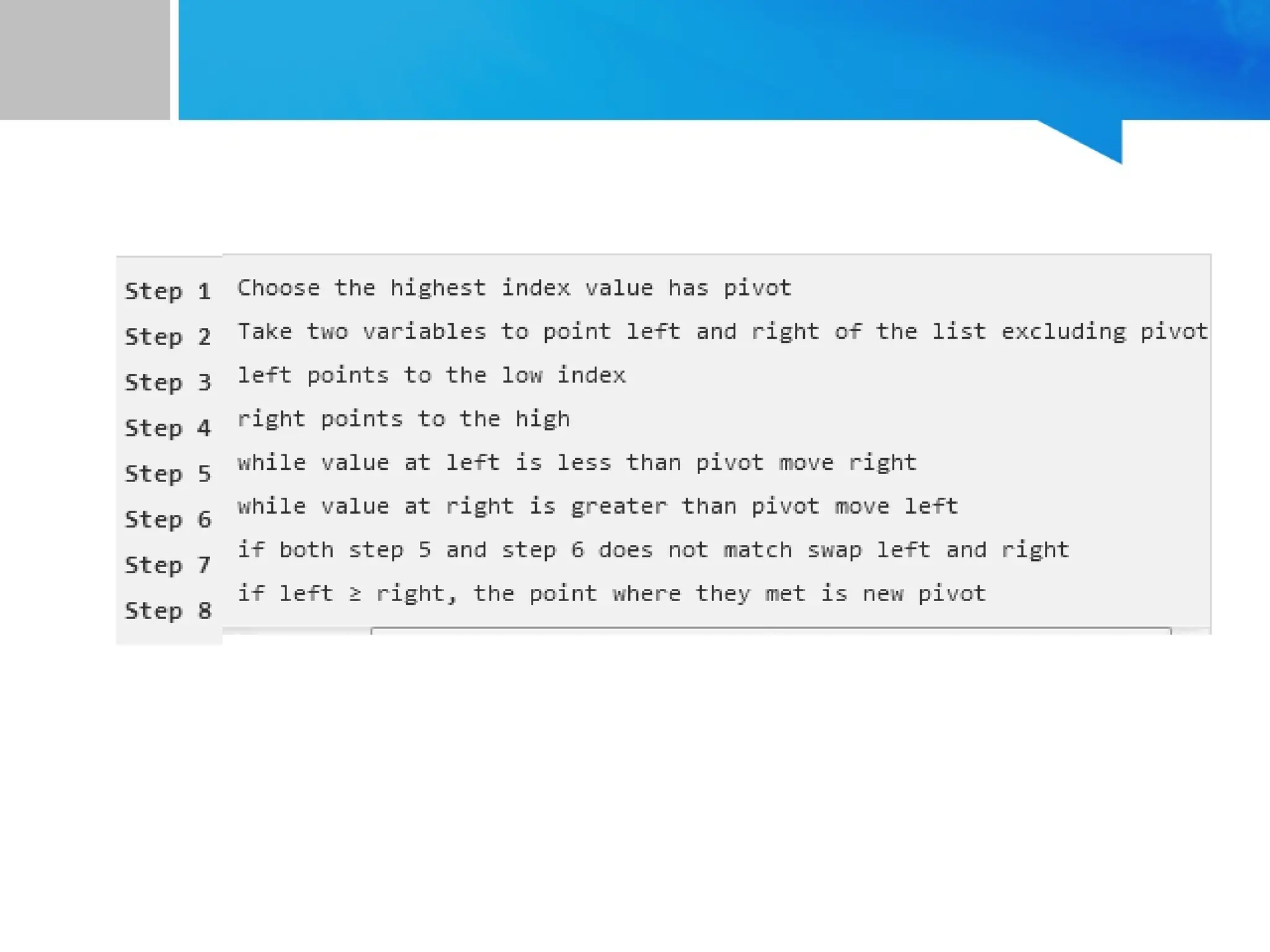
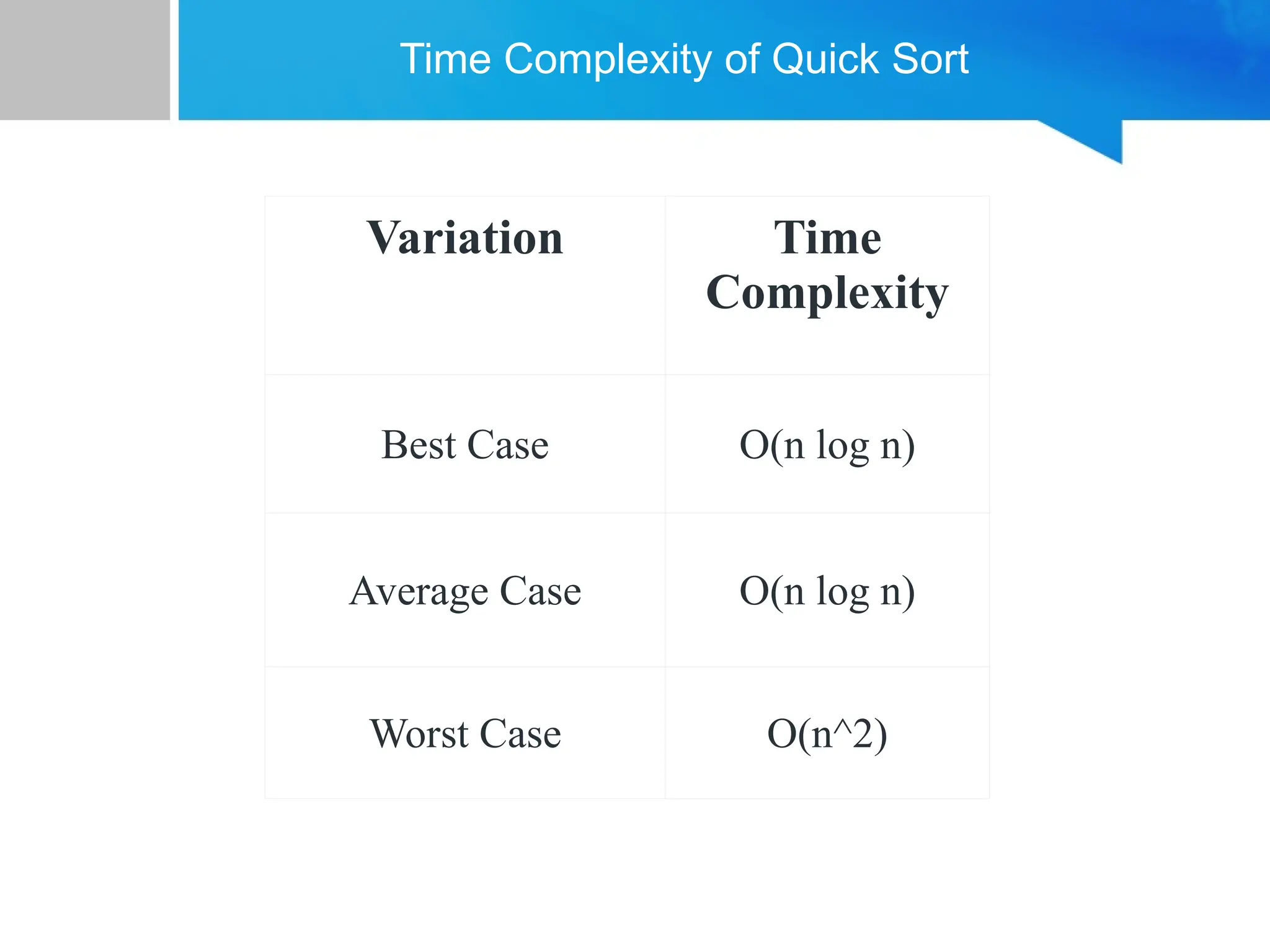

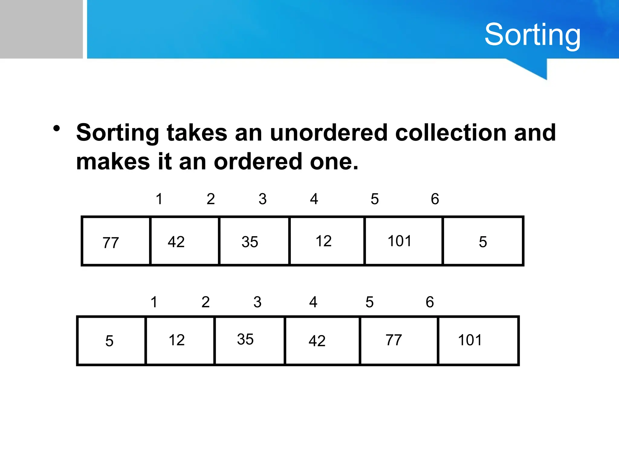
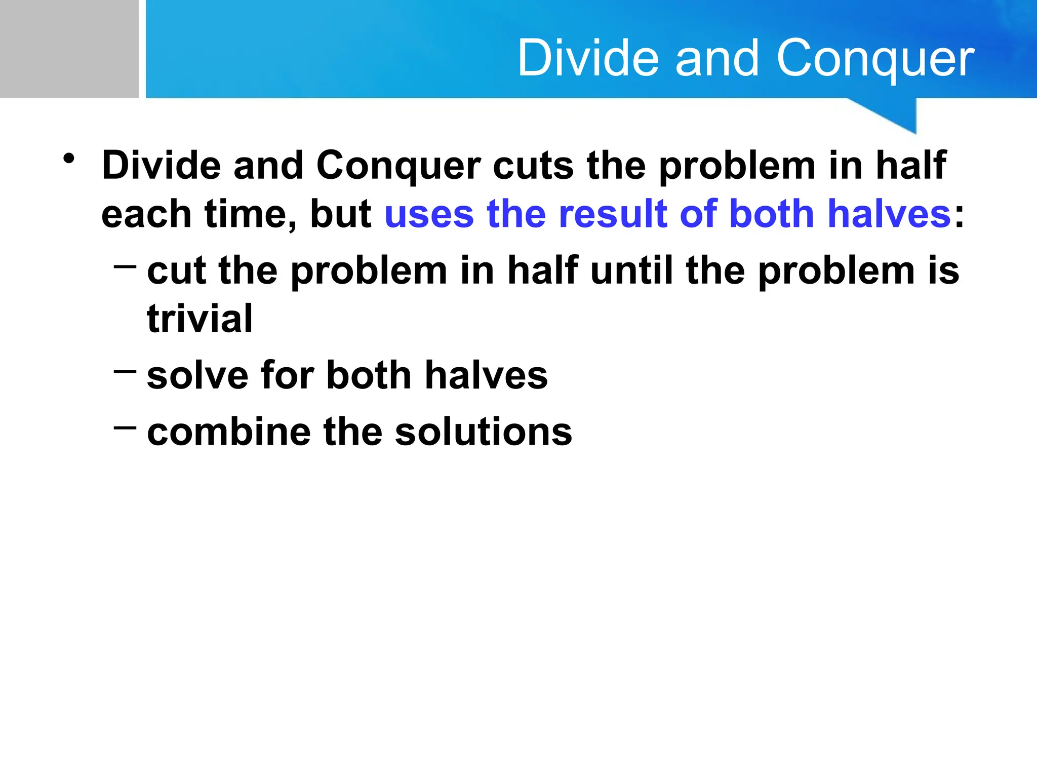
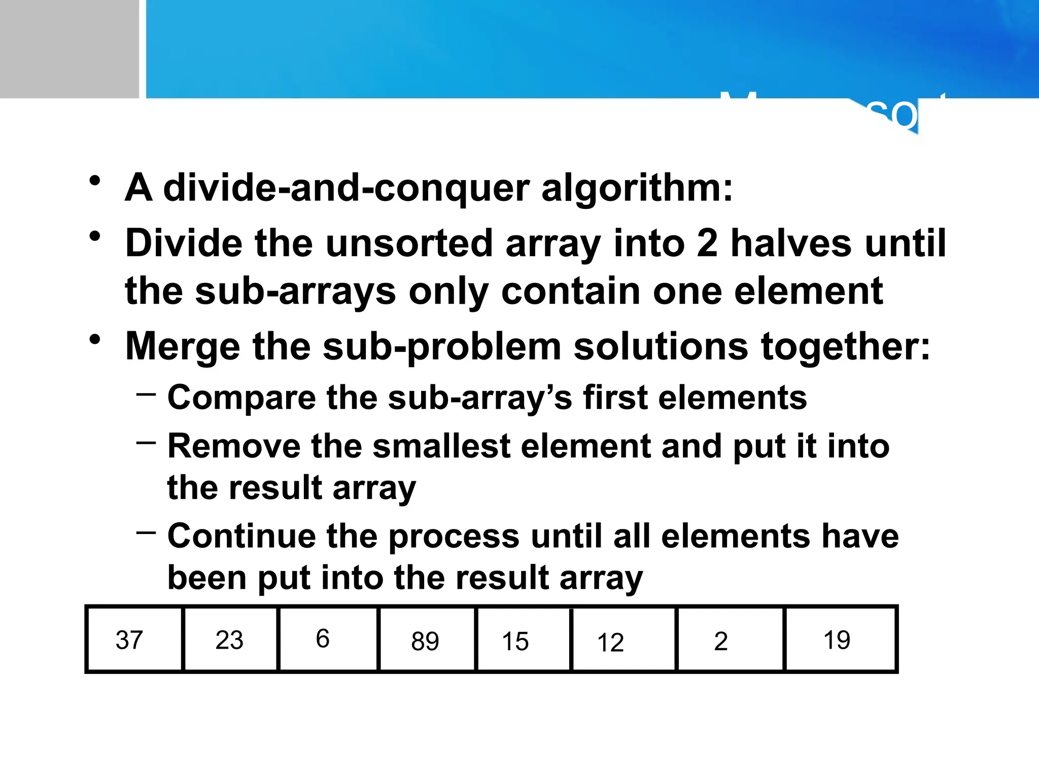
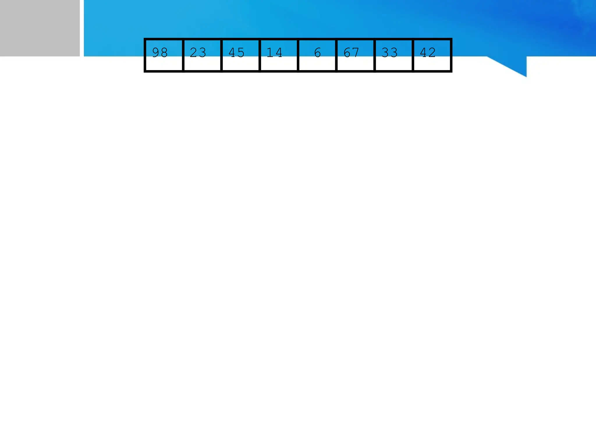
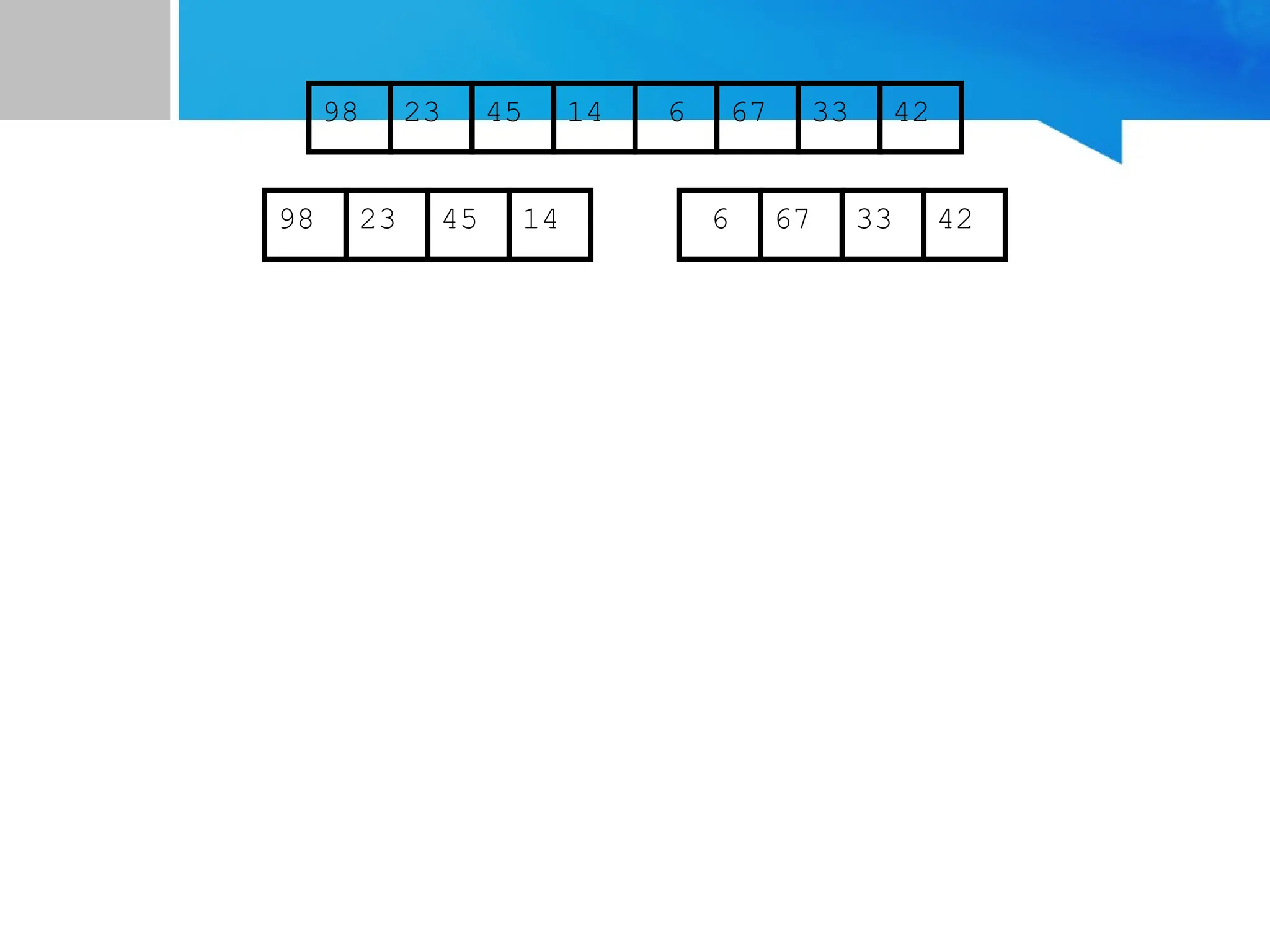
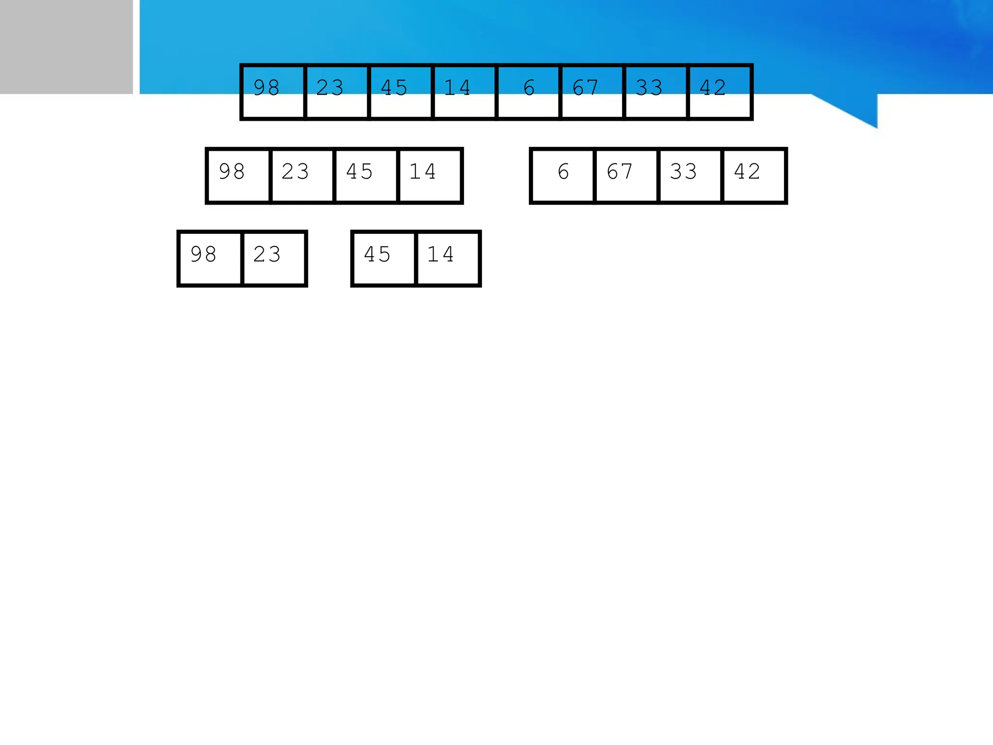

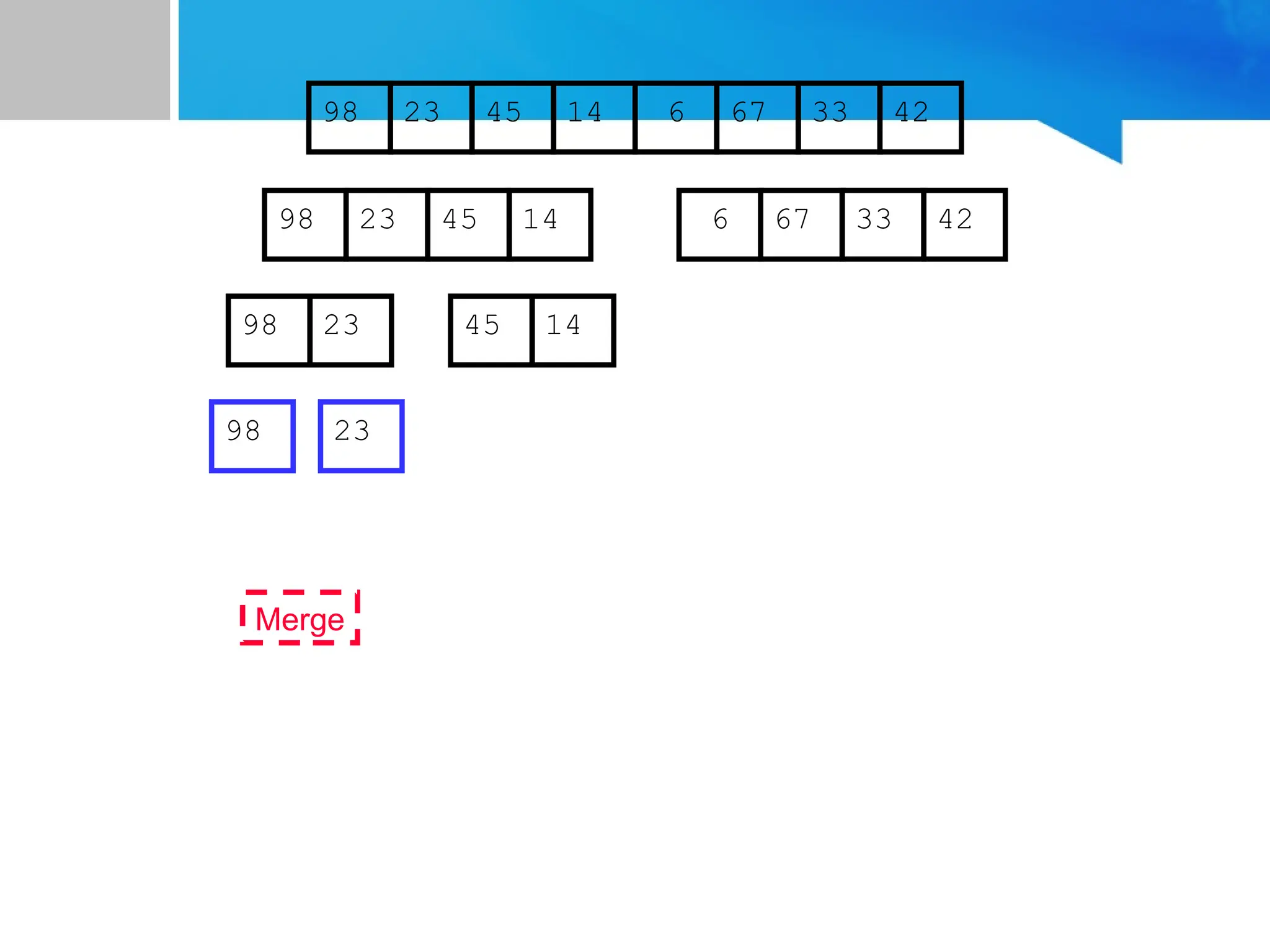
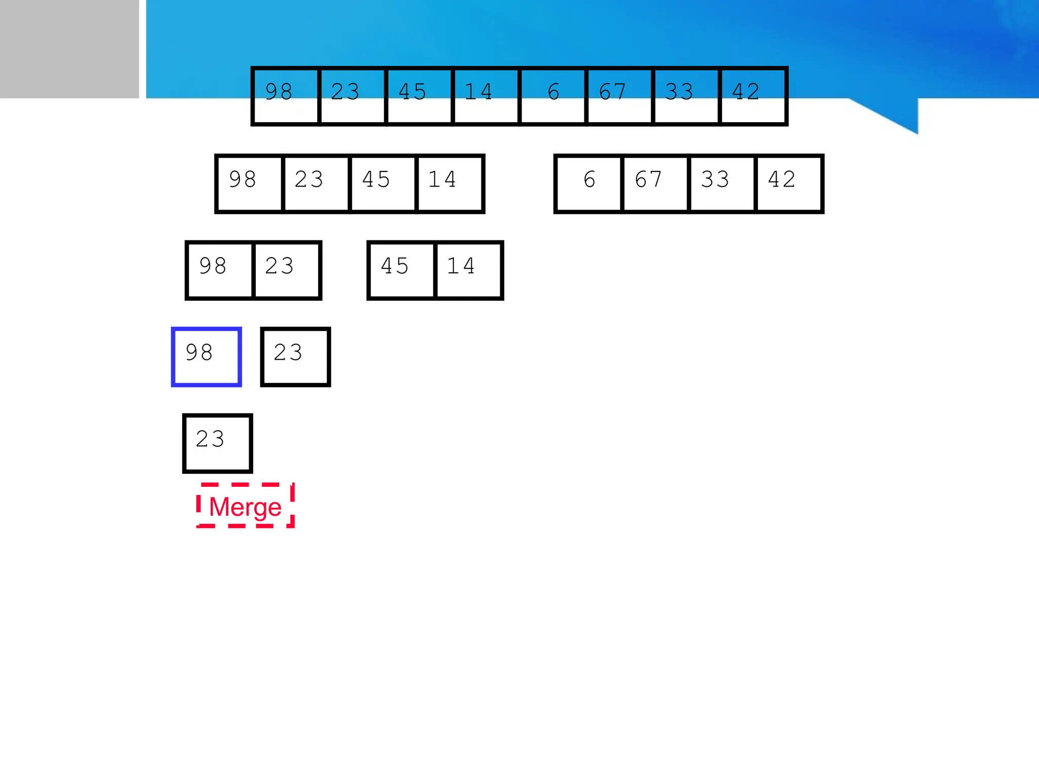

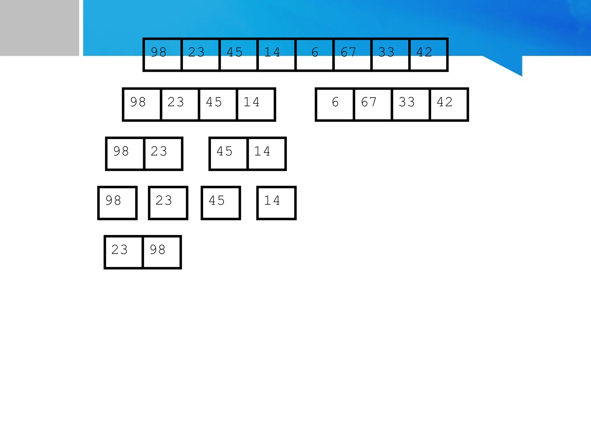
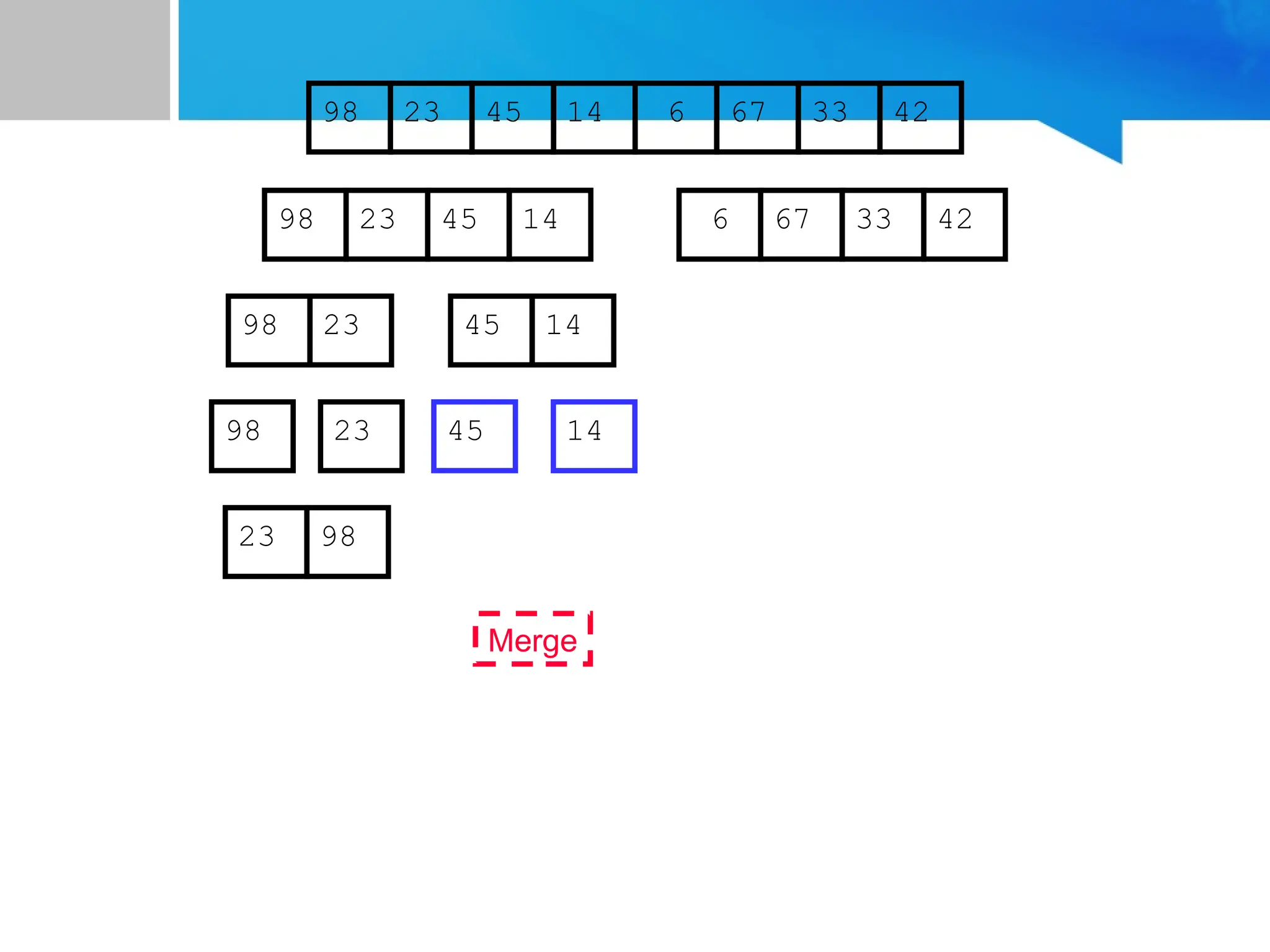
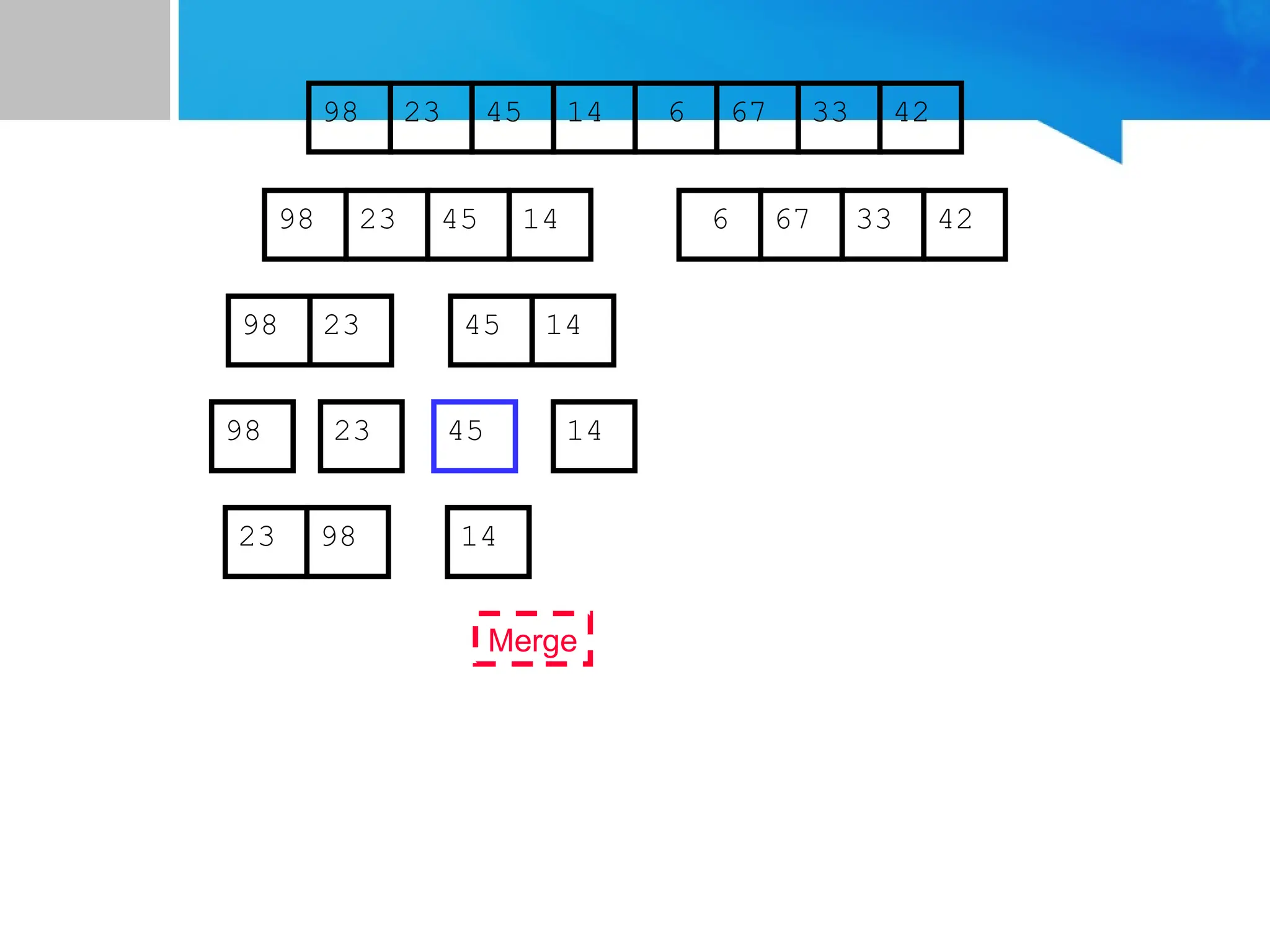
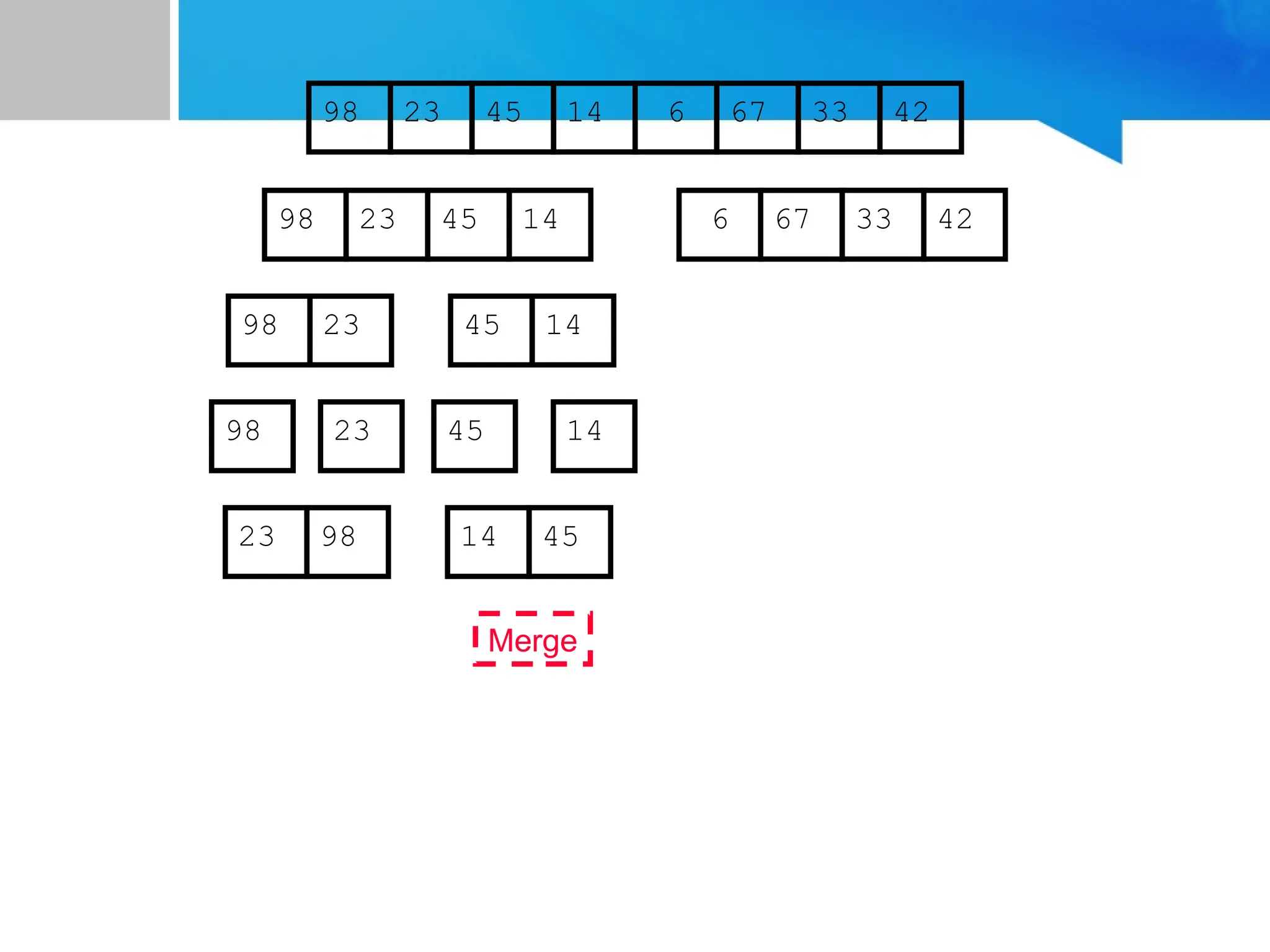
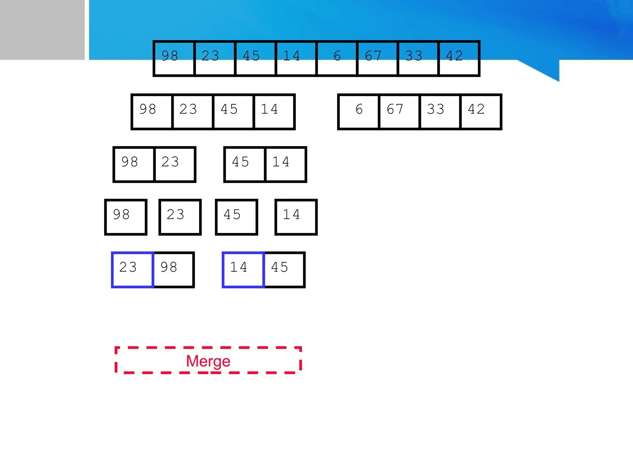
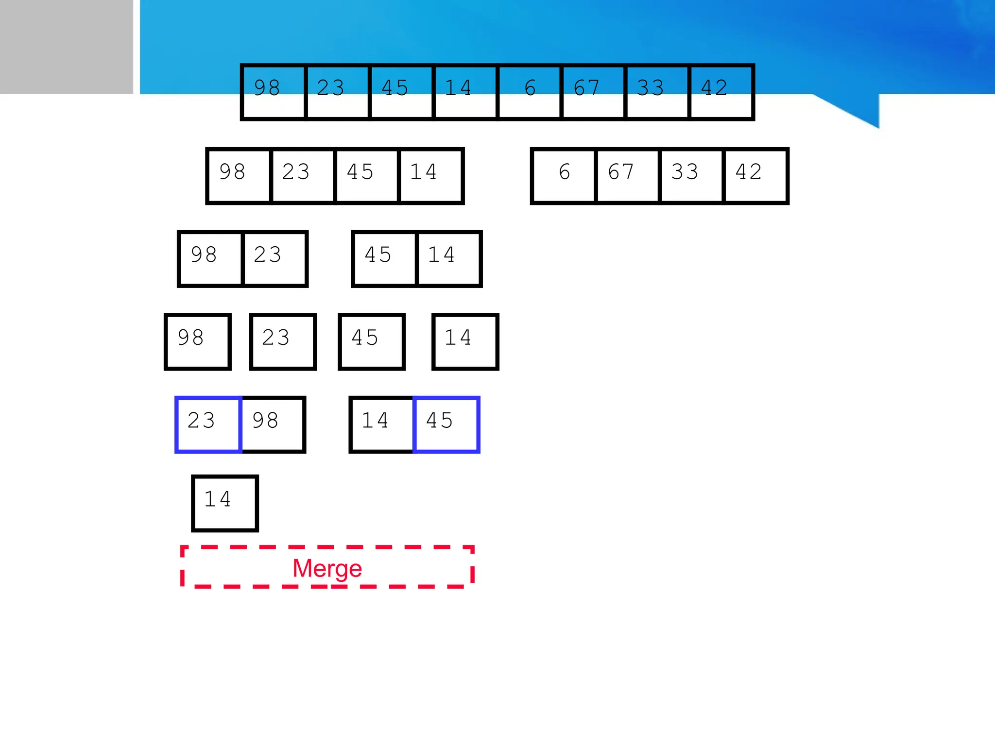


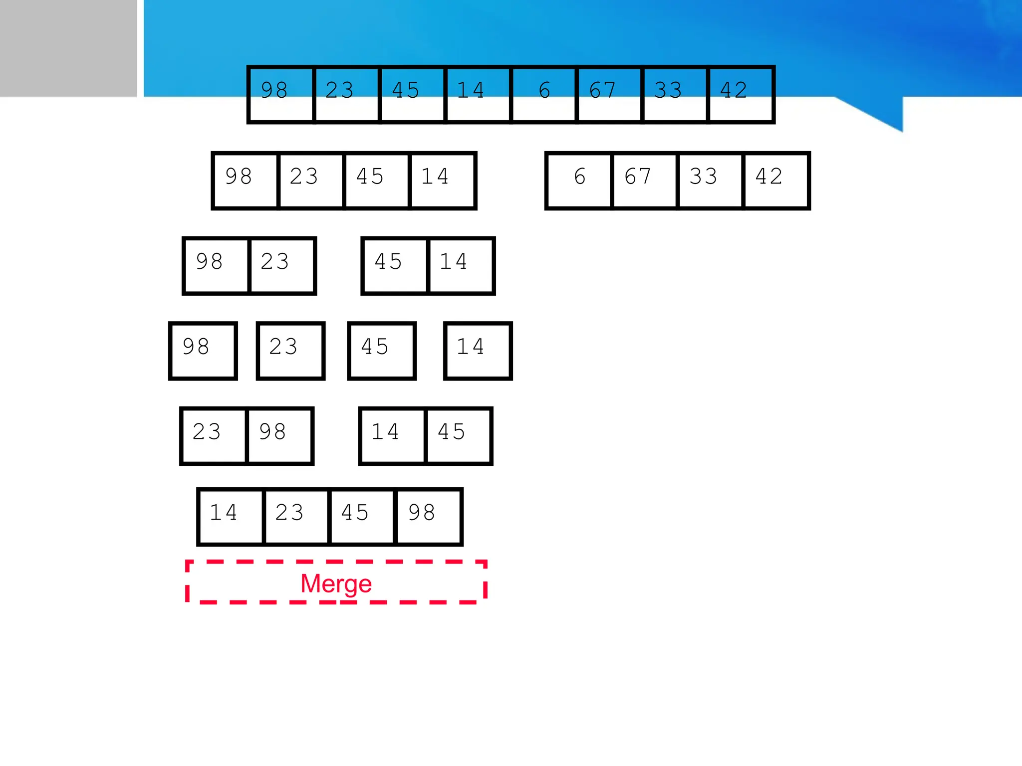
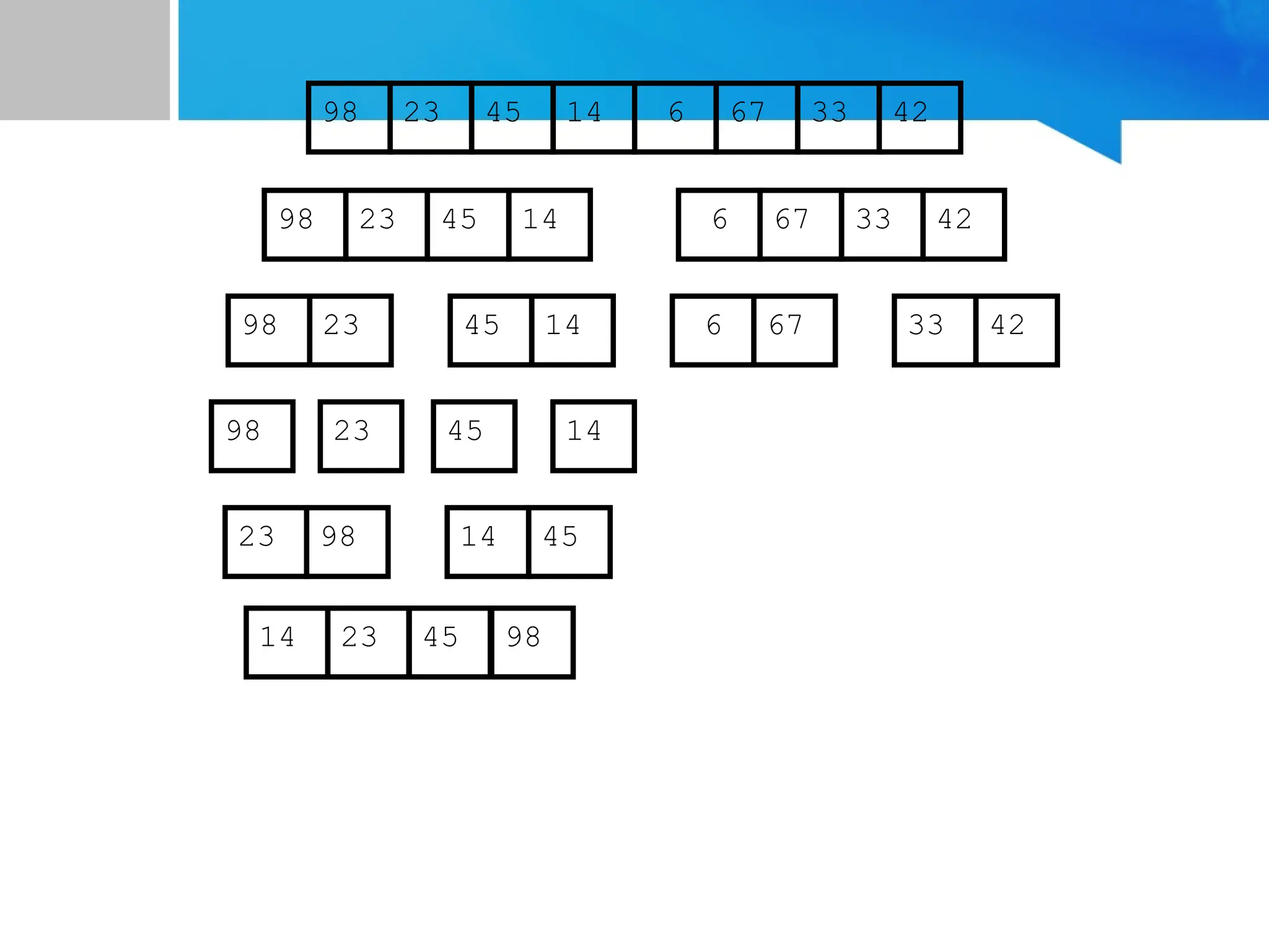
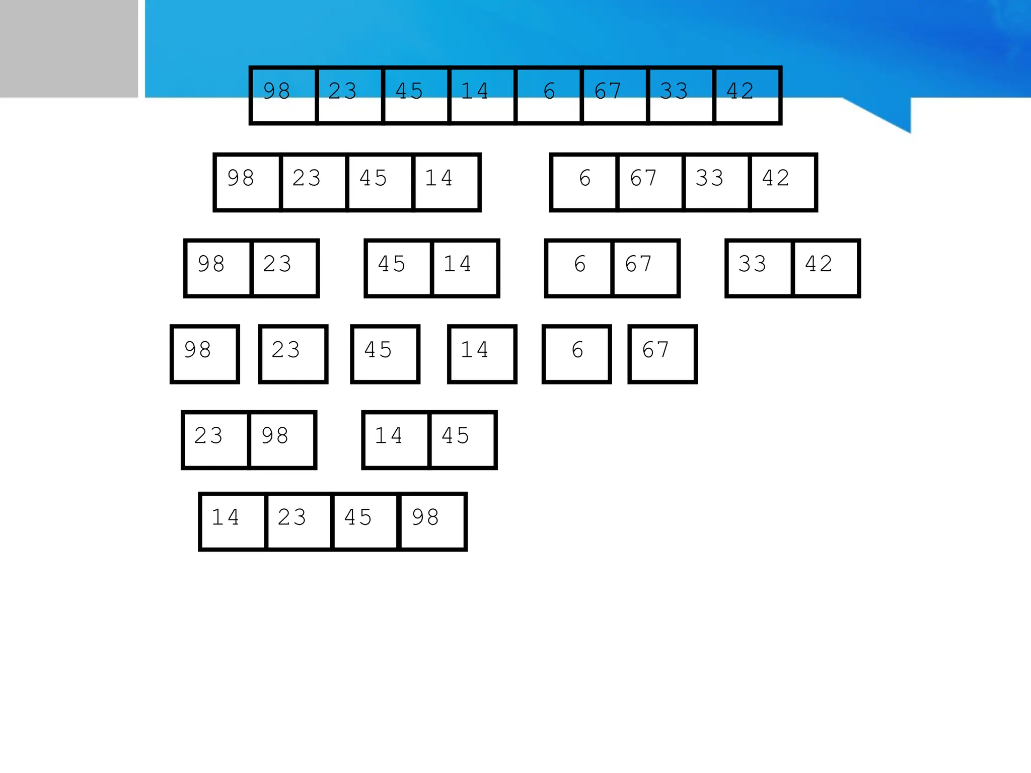
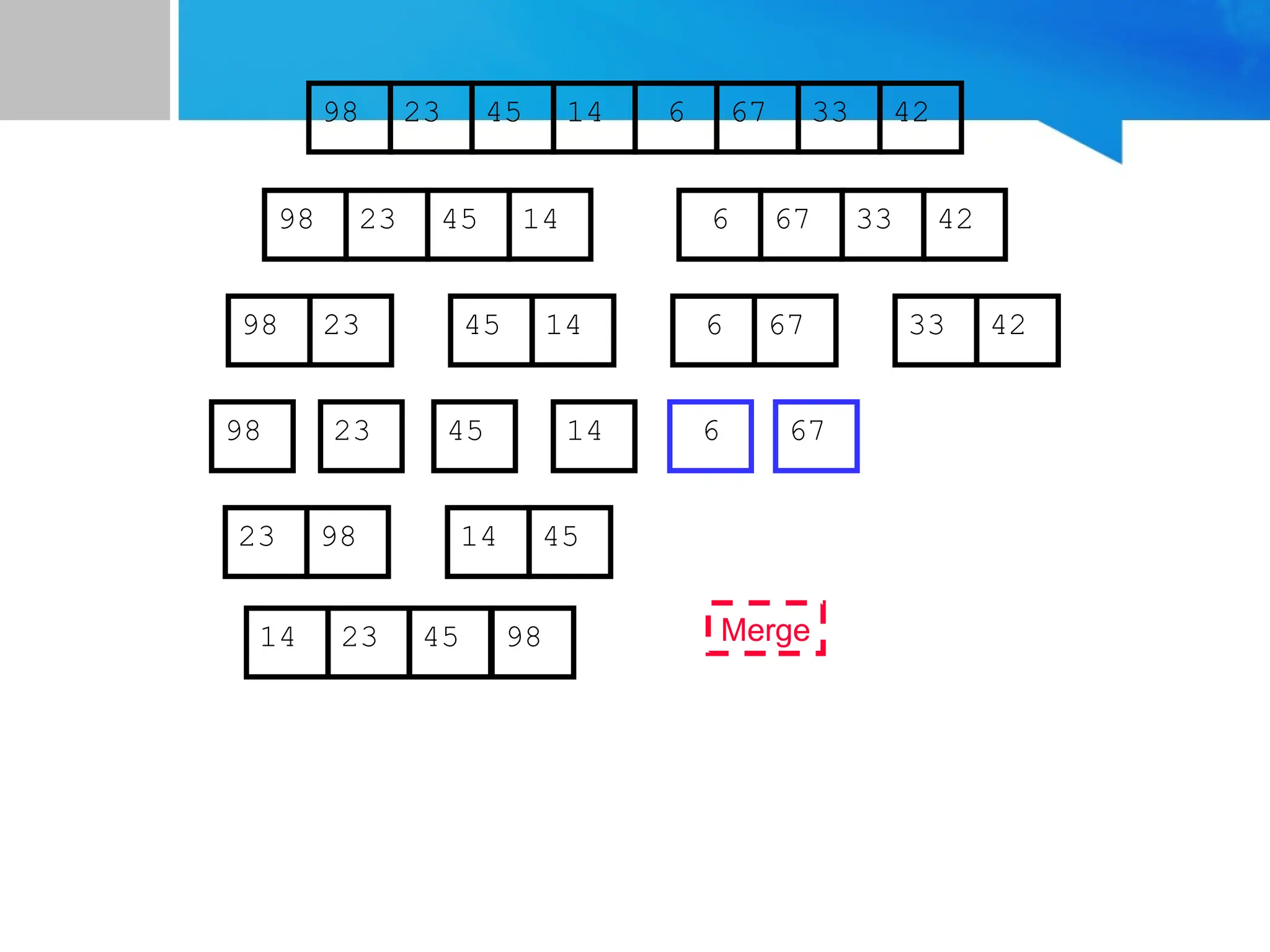

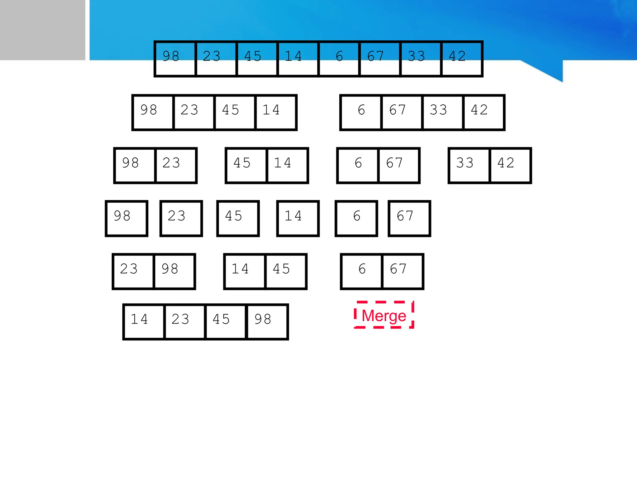

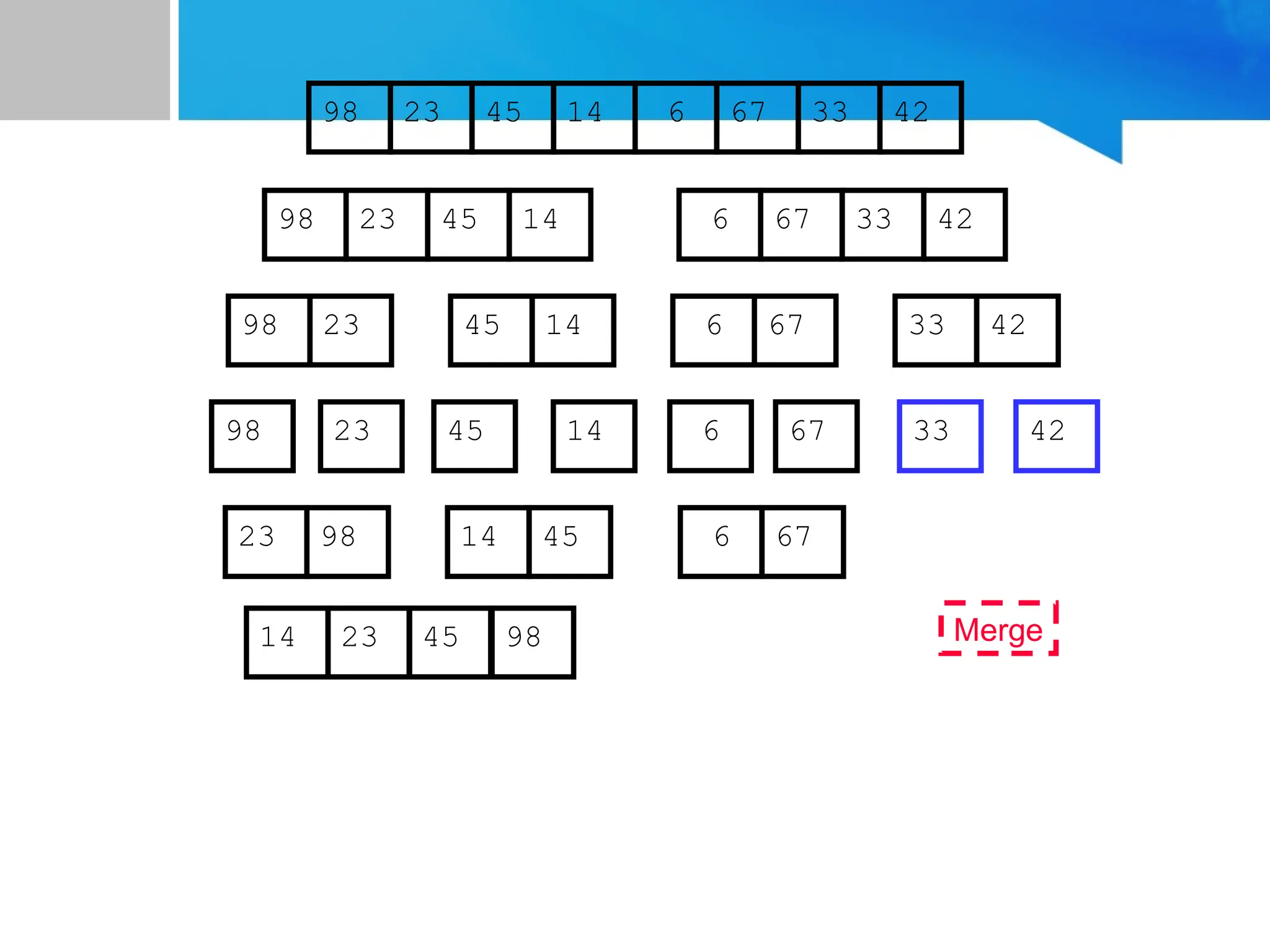
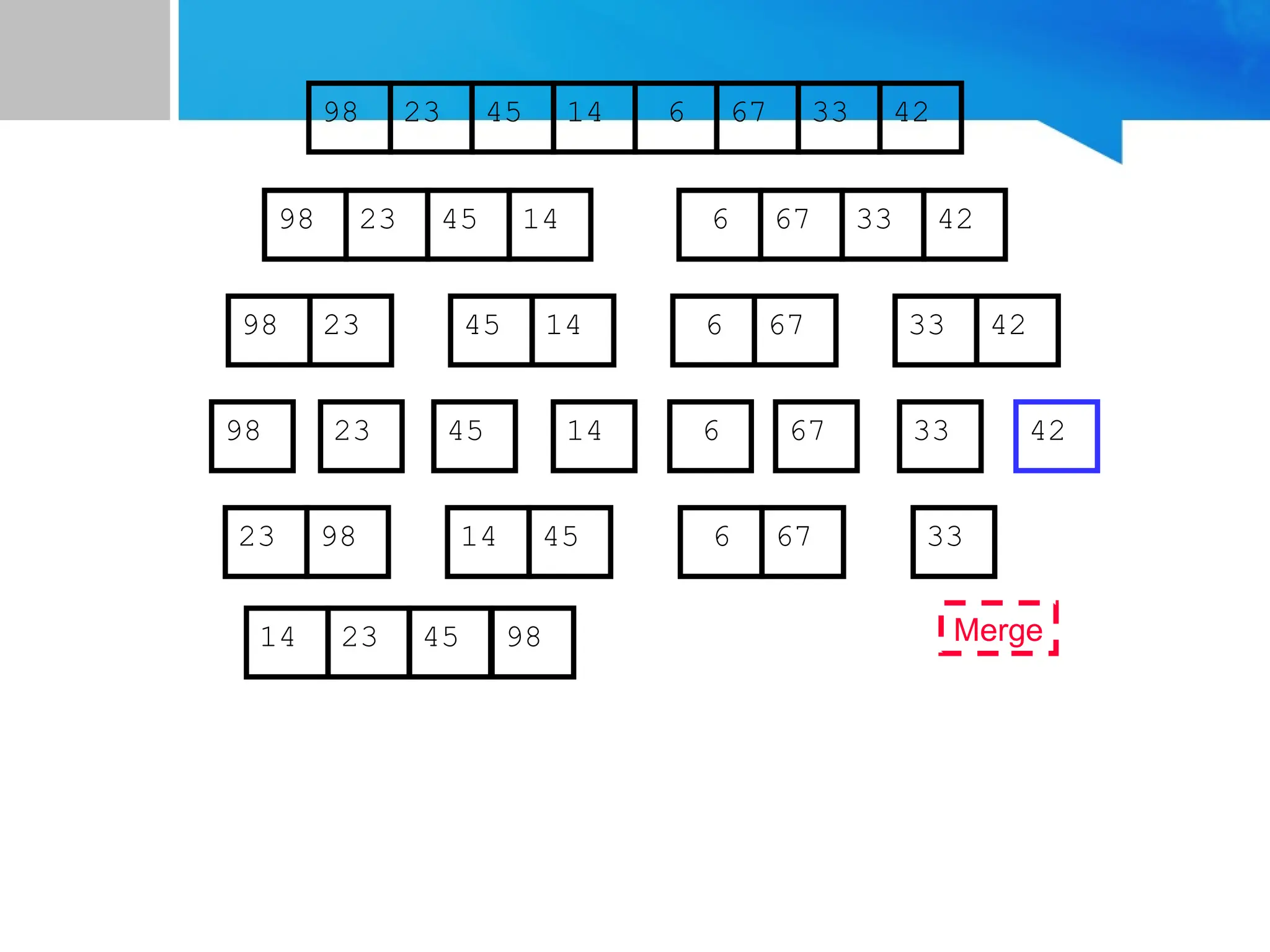

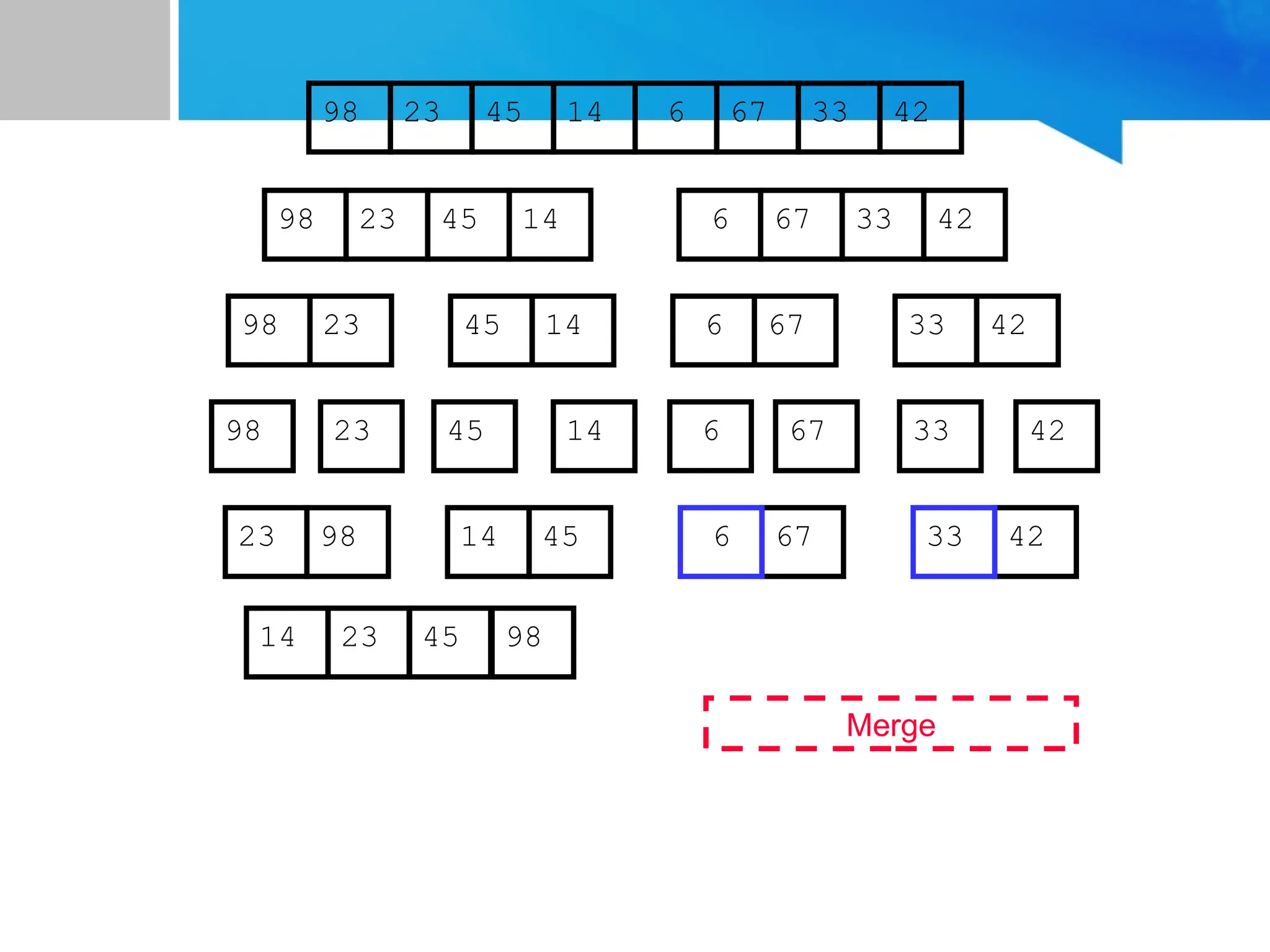

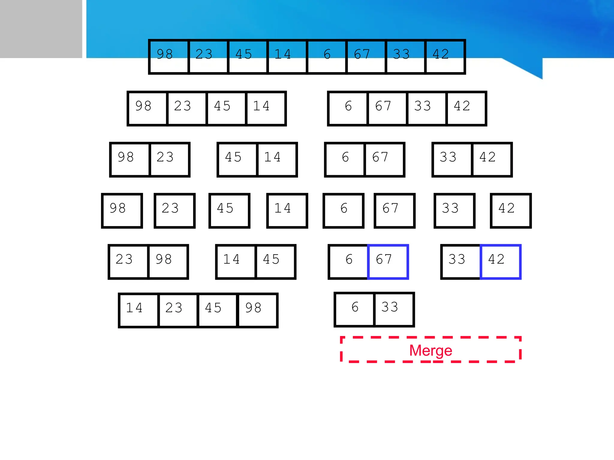
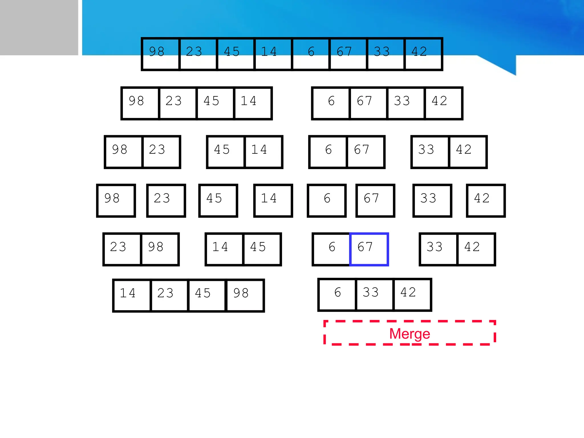

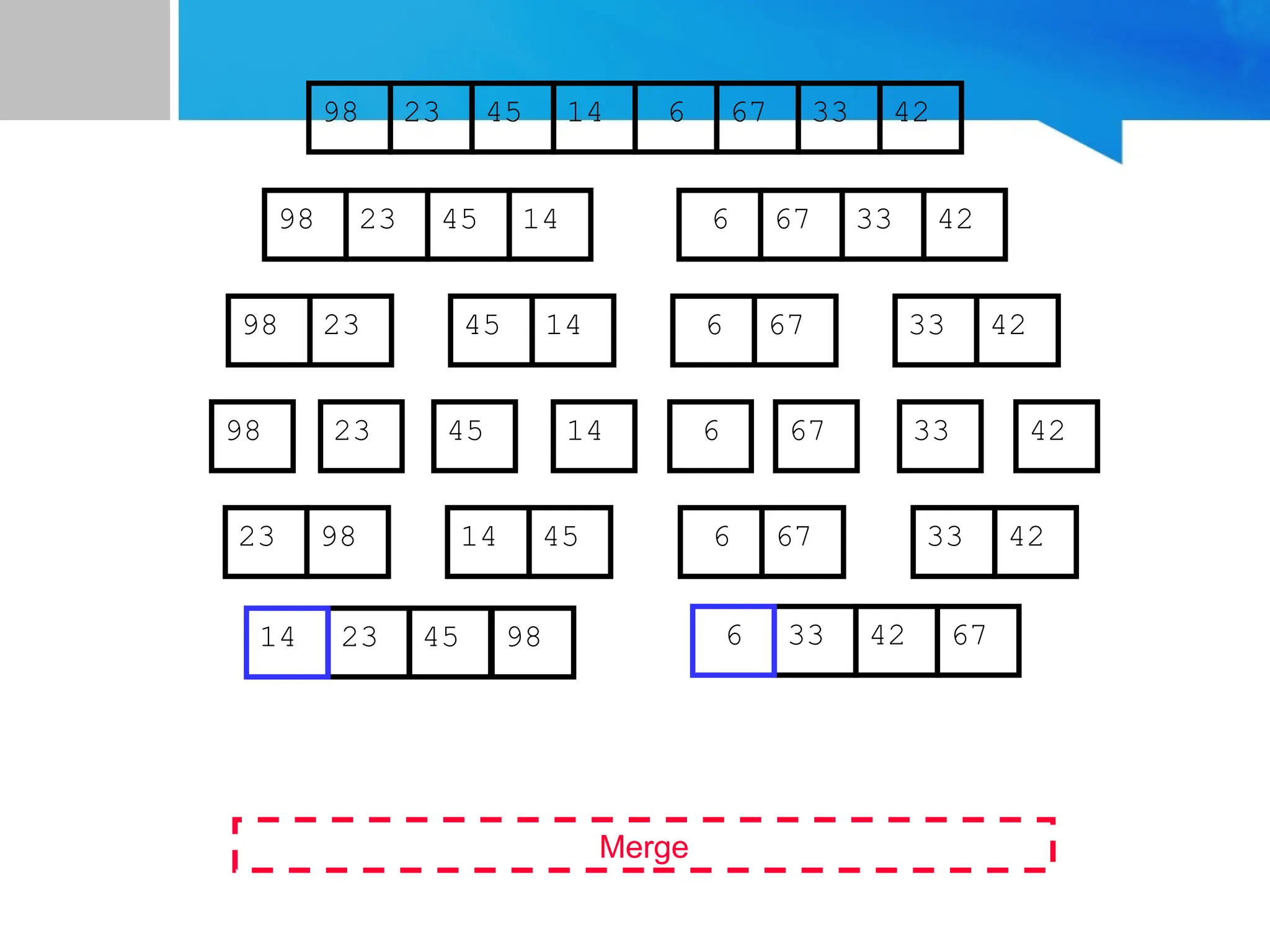

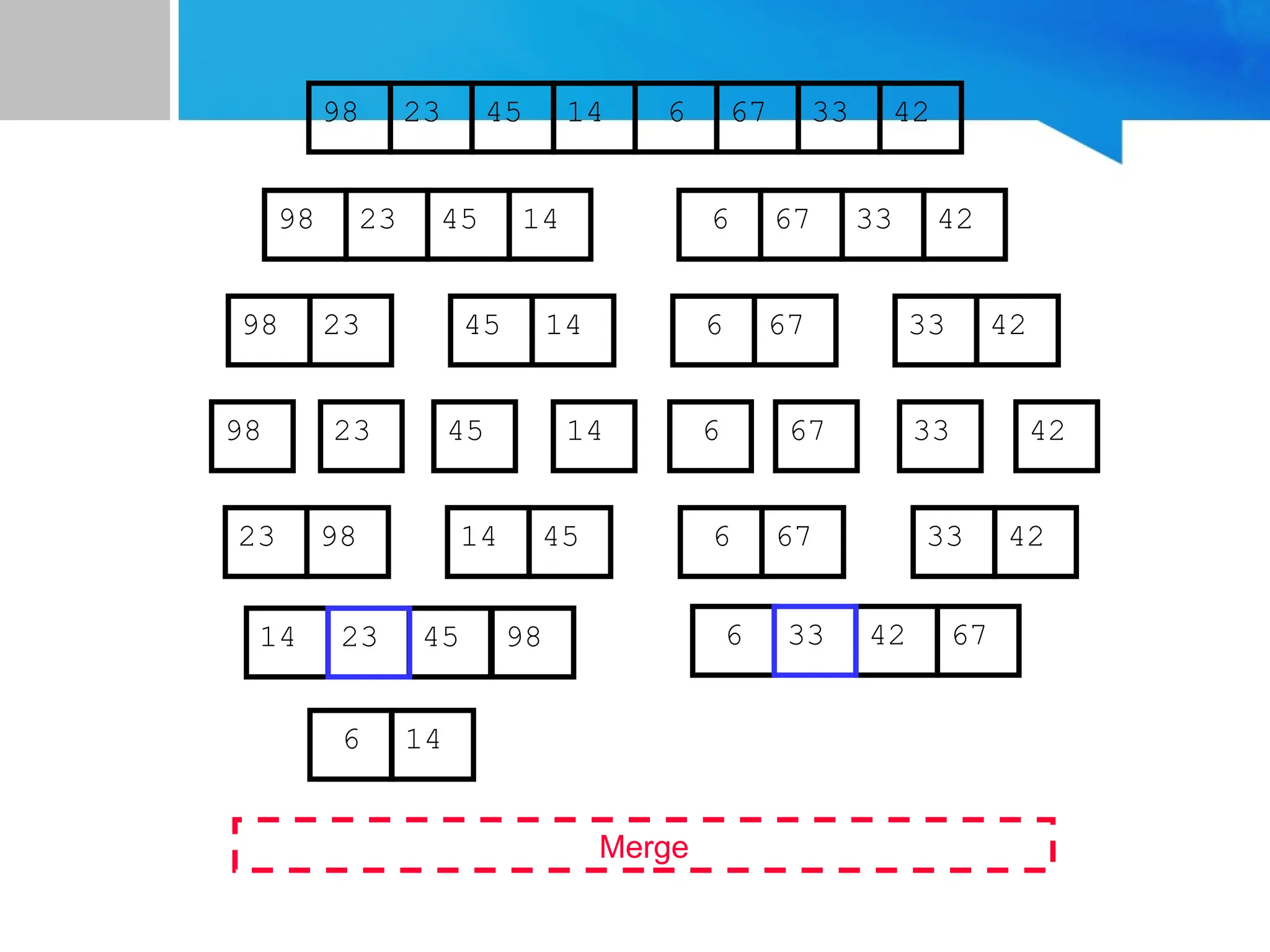
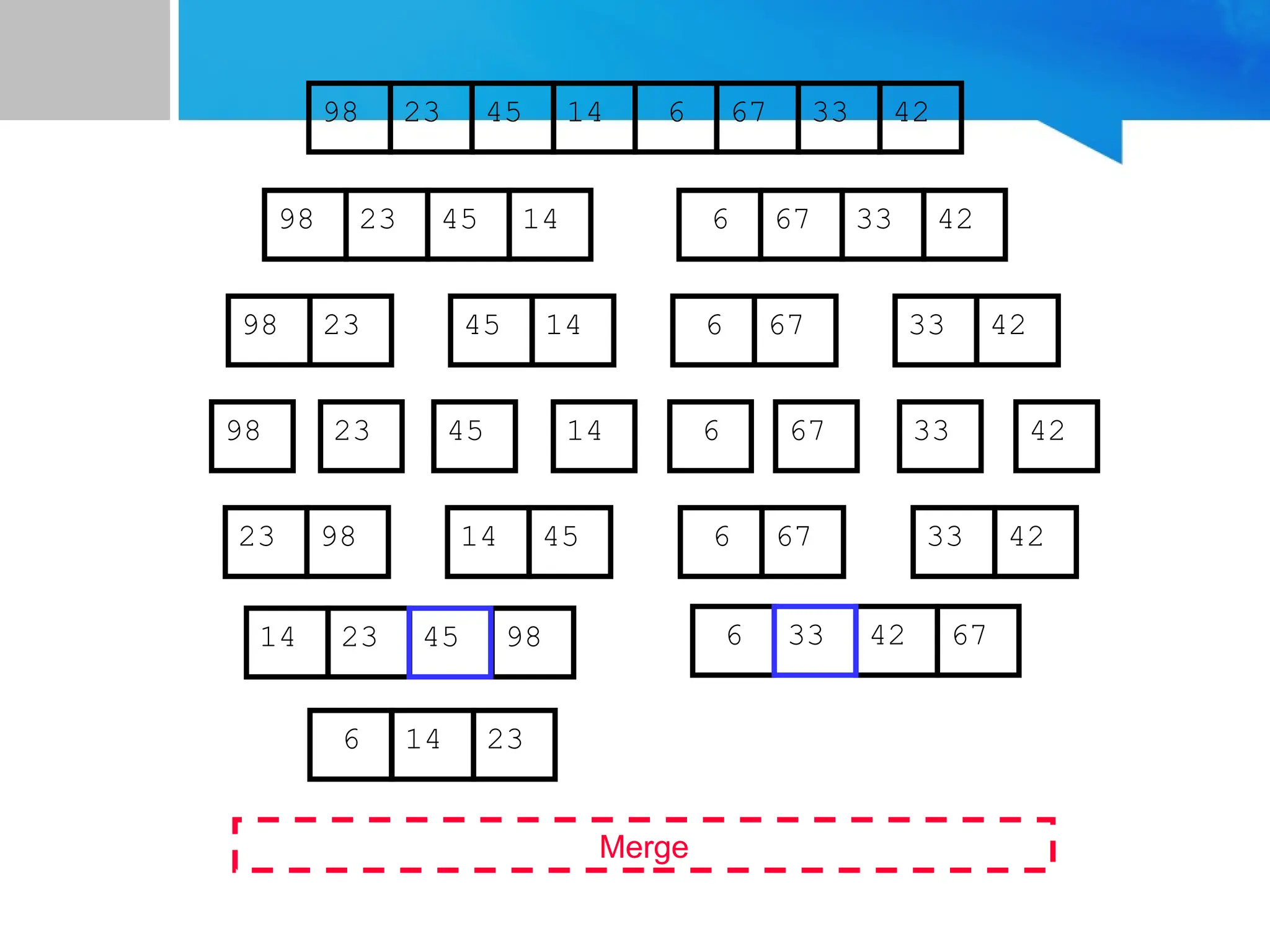

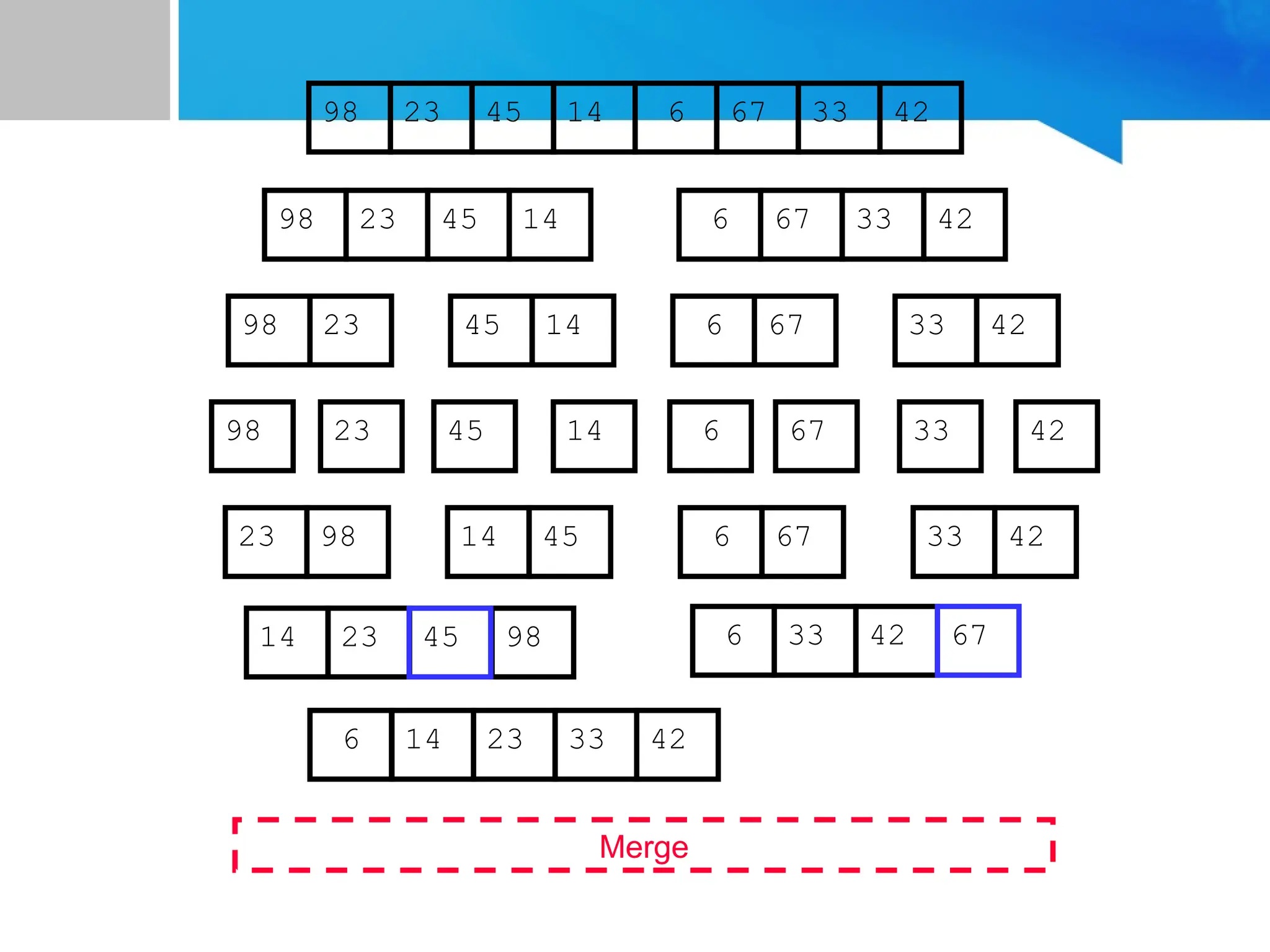
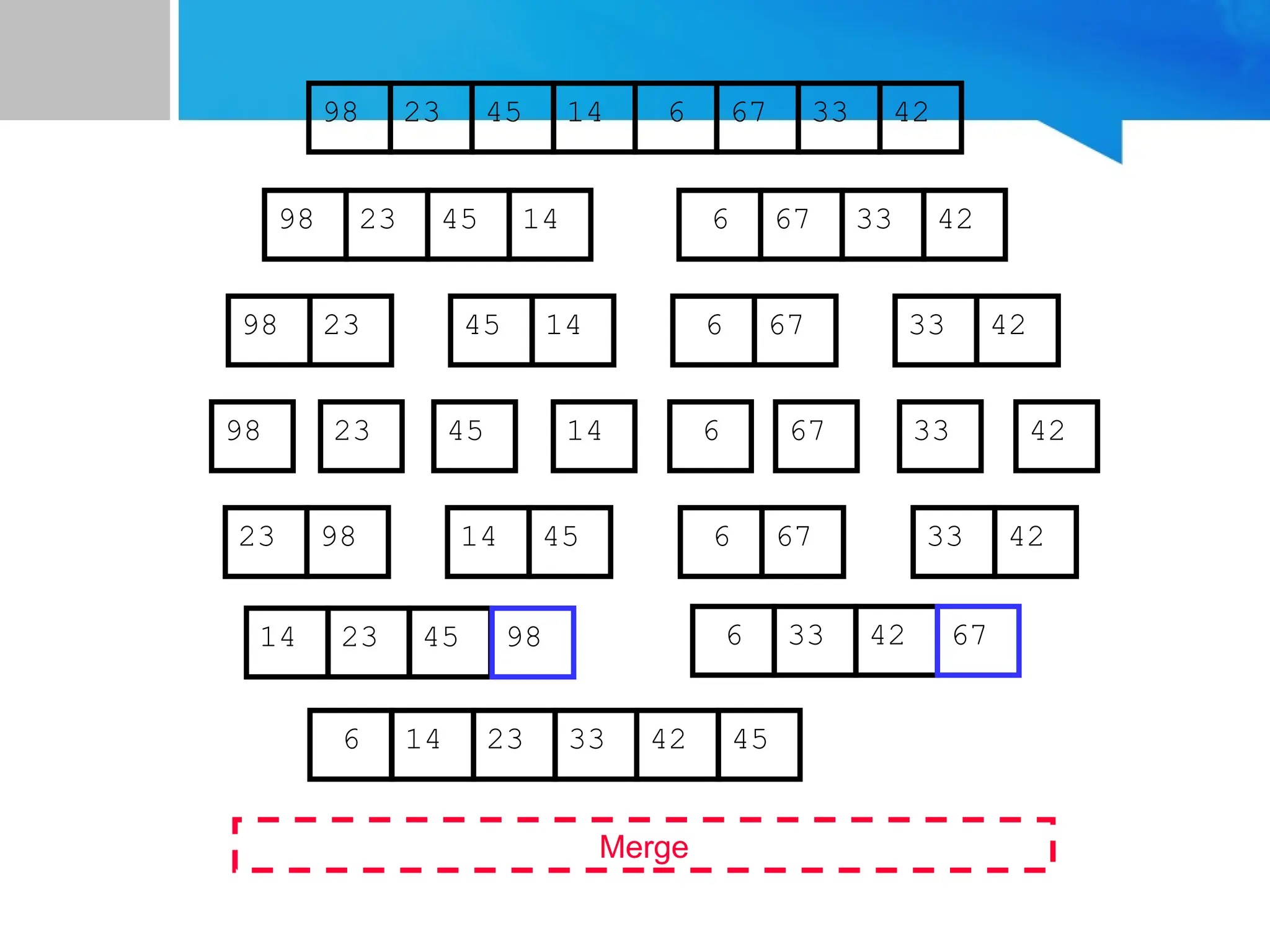
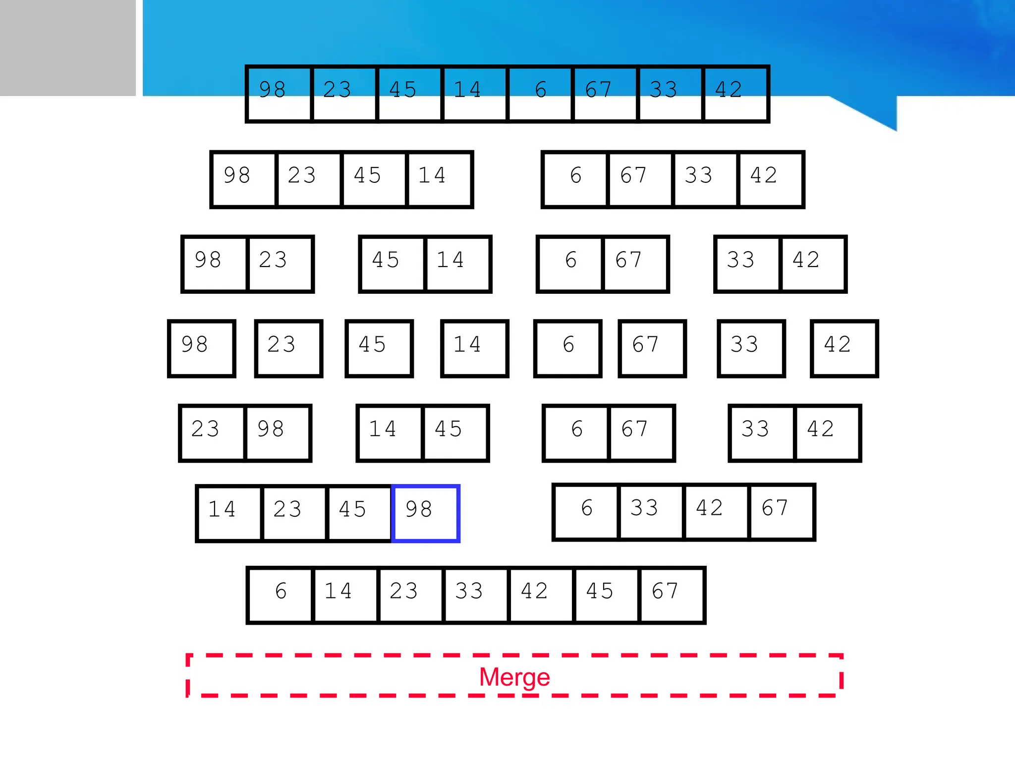
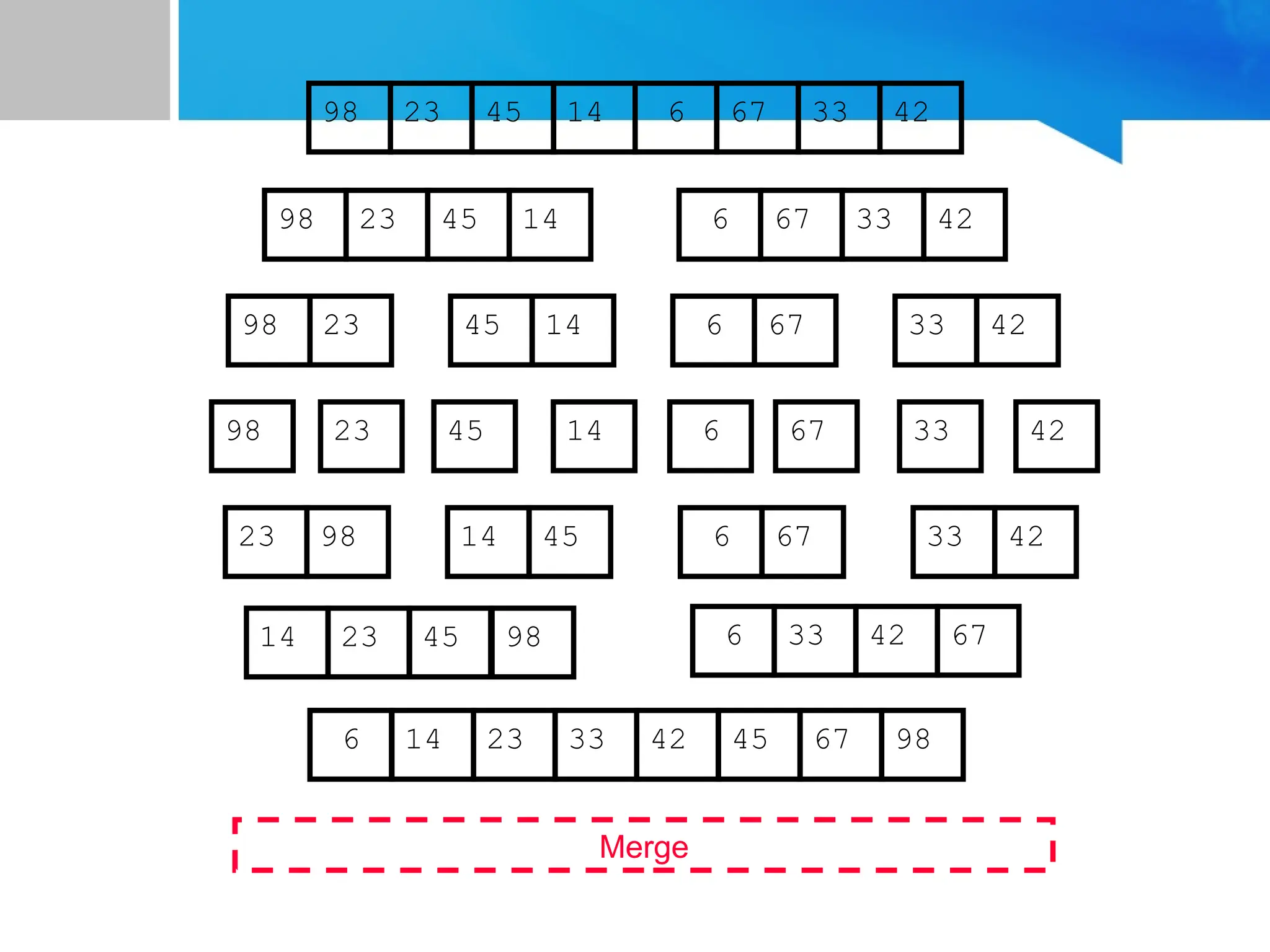
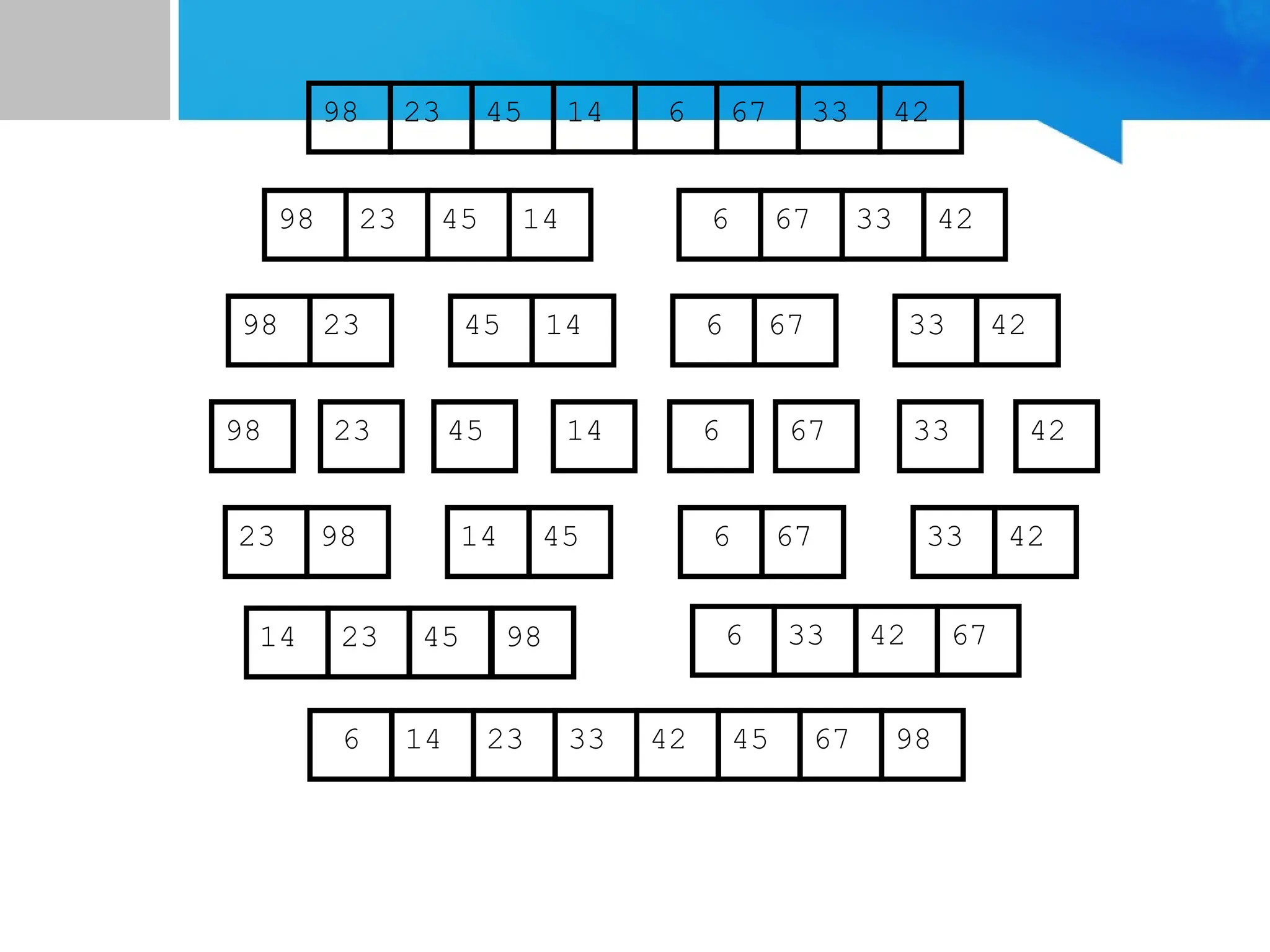
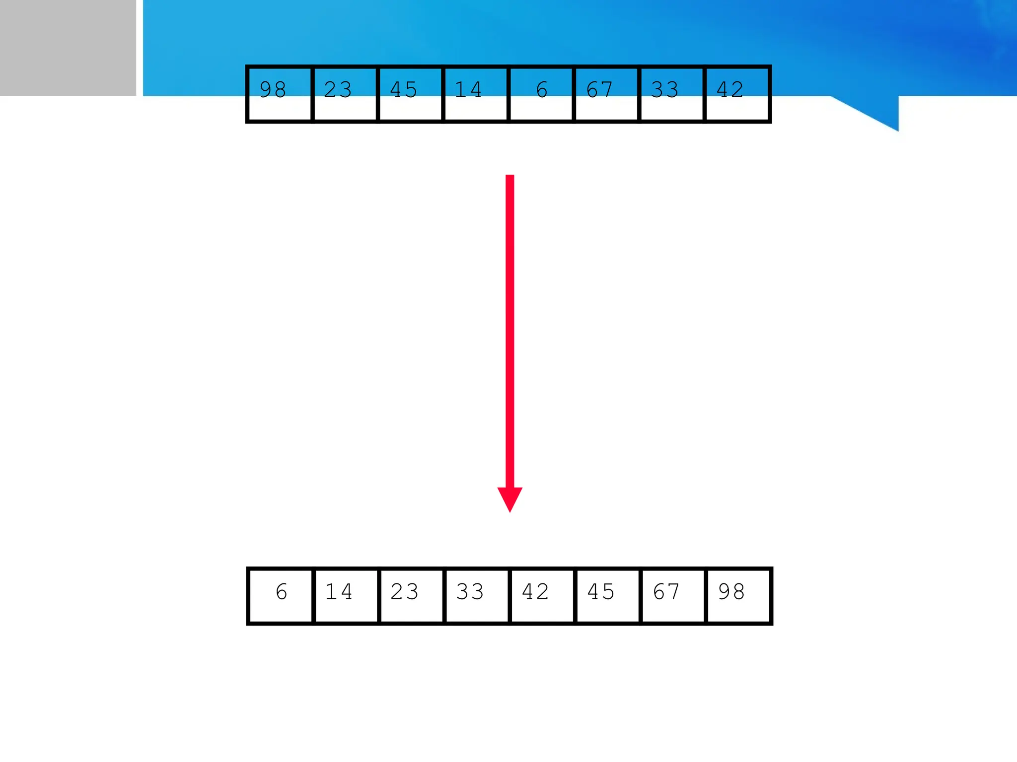
![// The subarray to be sorted is in the index range [left-right]
void mergeSort(int arr[], int left, int right) {
if (left < right) {
// Calculate the midpoint
int mid = (right + left) / 2;
// Sort first and second halves
mergeSort(arr, left, mid);
mergeSort(arr, mid + 1, right);
// Merge the sorted halves
merge(arr, left, mid, right);
}](https://image.slidesharecdn.com/datastructuressearchingandsorting-250503115212-17f1421f/75/Data-Structures_Searching-and-Sorting-pptx-149-2048.jpg)
![void merge(int arr[], int left, int mid, int right) {
int i, j, k;
int n1 = mid - left + 1;
int n2 = right - mid;
// Create temporary arrays
int leftArr[n1], rightArr[n2];
// Copy data to temporary arrays
for (i = 0; i < n1; i++)
leftArr[i] = arr[left + i];
for (j = 0; j < n2; j++)
rightArr[j] = arr[mid + 1 + j];](https://image.slidesharecdn.com/datastructuressearchingandsorting-250503115212-17f1421f/75/Data-Structures_Searching-and-Sorting-pptx-150-2048.jpg)
![// Merge the temporary arrays back
into arr[left..right]
i = 0;
j = 0;
k = left;
while (i < n1 && j < n2) {
if (leftArr[i] <= rightArr[j]) {
arr[k] = leftArr[i];
i++;
}
else {
arr[k] = rightArr[j];
j++;
}
k++;
}
// Copy the remaining elements of leftArr[], if any
while (i < n1) {
arr[k] = leftArr[i];
i++;
k++;
}
// Copy the remaining elements of rightArr[], if any
while (j < n2) {
arr[k] = rightArr[j];
j++;
k++;
}
}](https://image.slidesharecdn.com/datastructuressearchingandsorting-250503115212-17f1421f/75/Data-Structures_Searching-and-Sorting-pptx-151-2048.jpg)

![Bucket Sort Algorithm:
The algorithm can be expressed as following:
1. Take the array then find the maximum and minimum elements of the array.
Find the range of each bucket.
Bucket range:((maximum element – minimum element)/number of elements)
2. Now insert the element into the bucket based on Bucket Index.
Bucket Index: floor(a[i]-minimum element)/range
3. Once the elements are inserted into each bucket, sort the elements within
each bucket using the insertion sort.](https://image.slidesharecdn.com/datastructuressearchingandsorting-250503115212-17f1421f/75/Data-Structures_Searching-and-Sorting-pptx-155-2048.jpg)
![Consider an array arr[] = {22, 72, 62, 32, 82, 142}
Range= (maximum-minimum) / number of elements
So, here the range will be given as: Range = (142 – 22)/6 = 20
Thus, the range of each bucket in bucket sort will be: 20 So, the buckets will
be as:
20-40; 40-60; 60-80; 80-100; 100-120; 120-140; 140-160
Bucket index = floor((a[i]-min)/range)
For 22, bucketindex = (22-22)/20 = 0.
For 72, bucketindex = (72-22)/20 = 2.5.
For 62, bucketindex = (62-22)/20 = 2.
For 32, bucketindex = (32-22)/20 = 0.5.
For 82, bucketindex = (82-22)/20 = 3.
For 142, bucketindex = (142-22)/20 = 6.](https://image.slidesharecdn.com/datastructuressearchingandsorting-250503115212-17f1421f/75/Data-Structures_Searching-and-Sorting-pptx-156-2048.jpg)
![Elements can be inserted into the bucket as:
0 -> 22 -> 32
1
2 -> 72 -> 62 (72 will be inserted before 62 as it appears first in the list).
3 -> 82
4
5
6 -> 142
Now sort the elements in each bucket using the insertion sort.
0 -> 22 -> 32
1
2 -> 62 -> 72
3 -> 82
4
5
6 -> 142
Now gather them together.
arr[] = {22, 32, 62, 72, 82, 142}](https://image.slidesharecdn.com/datastructuressearchingandsorting-250503115212-17f1421f/75/Data-Structures_Searching-and-Sorting-pptx-157-2048.jpg)