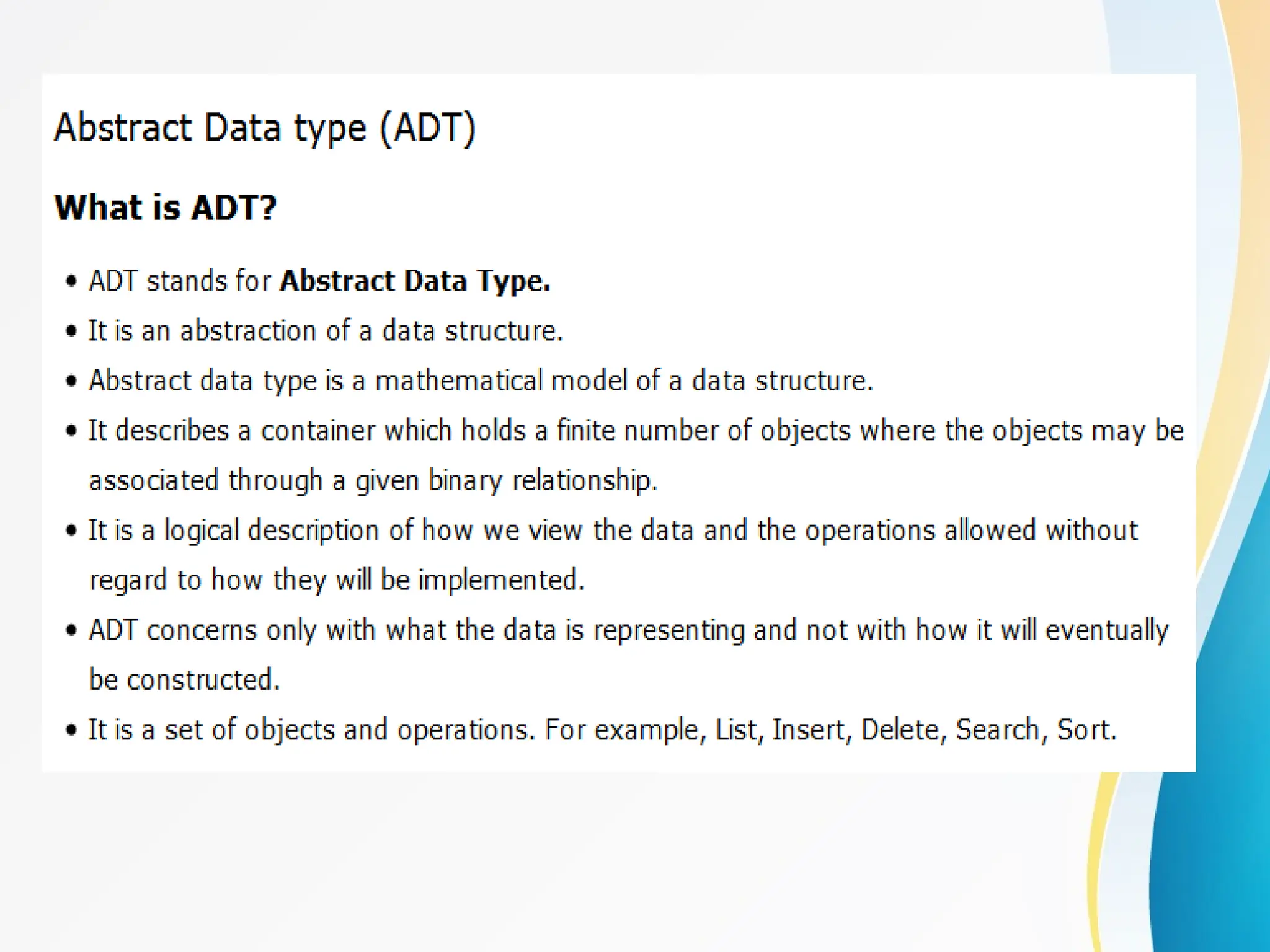
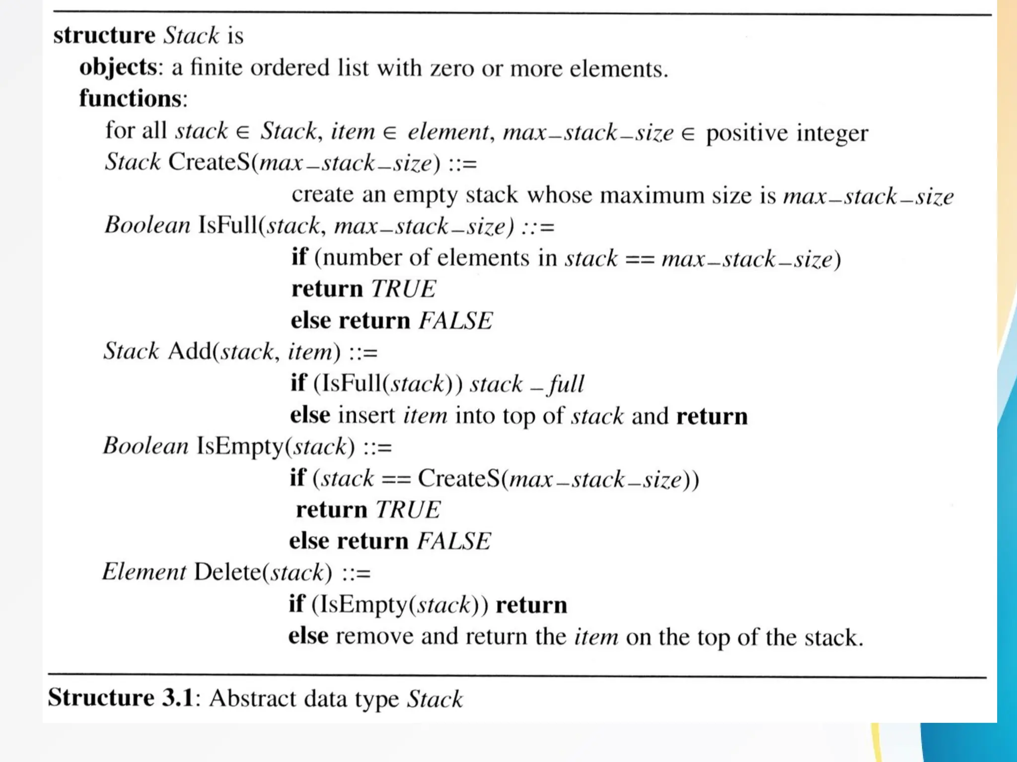
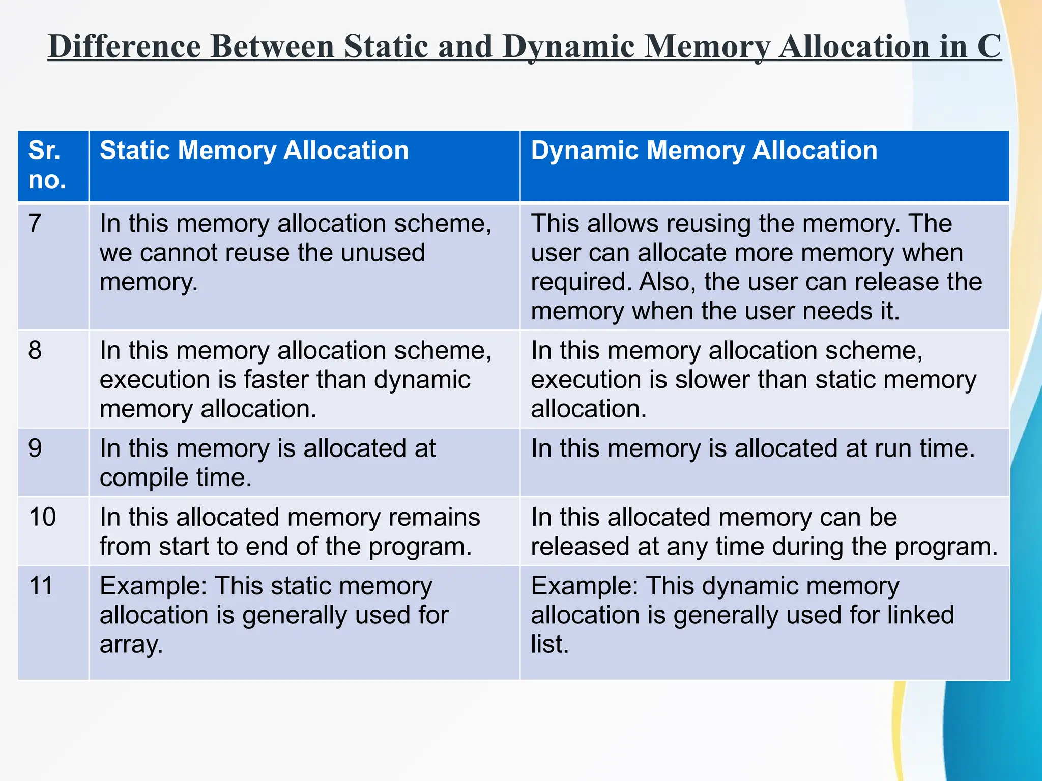
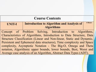
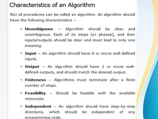
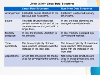
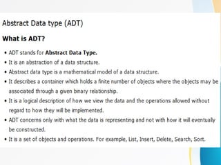
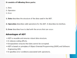
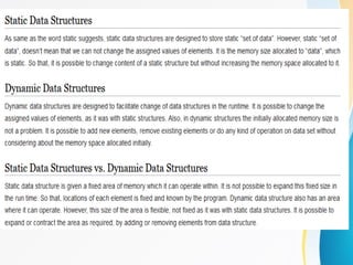
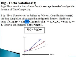
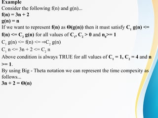
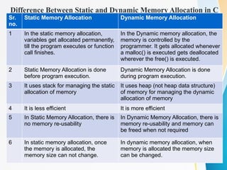
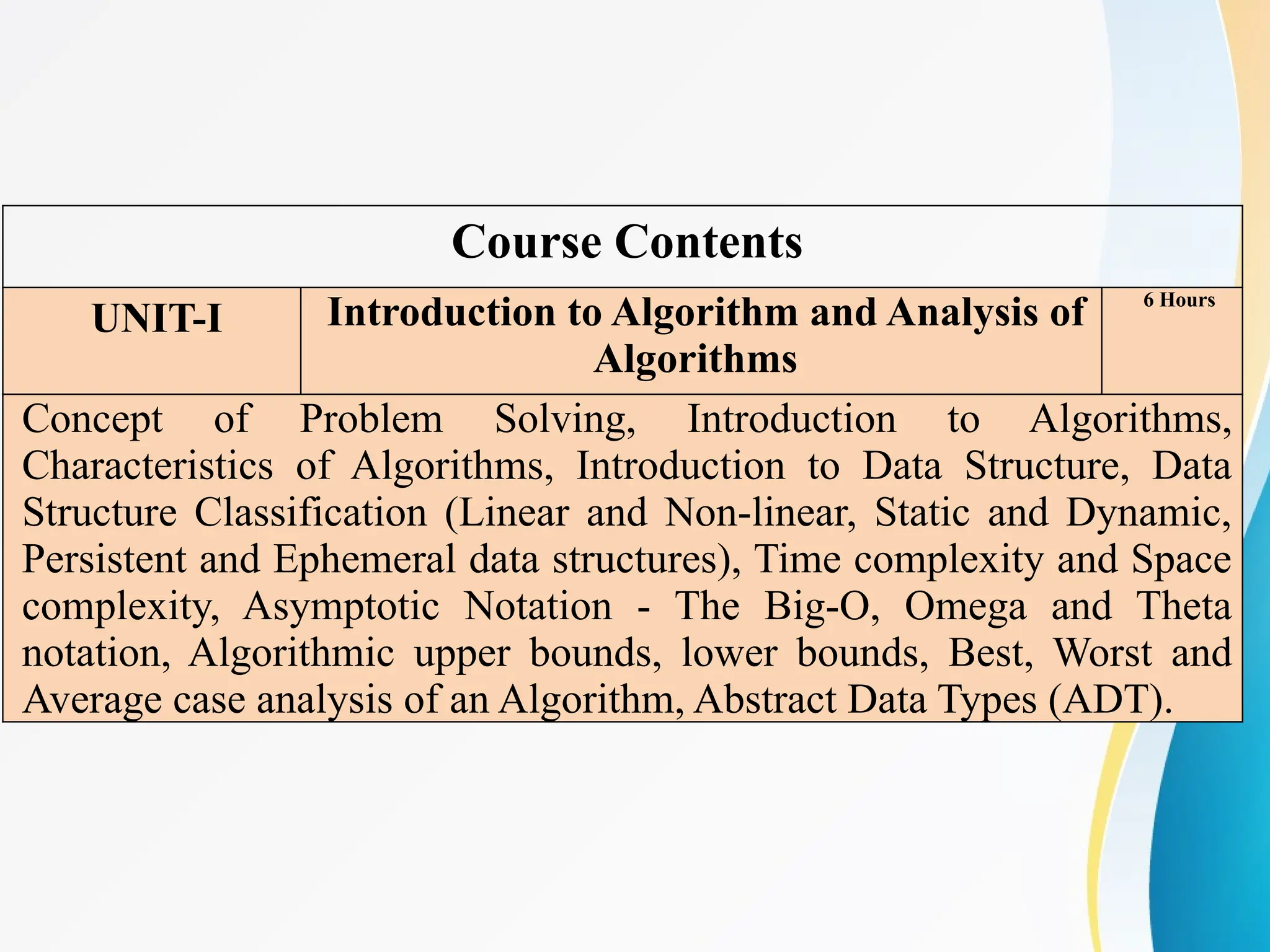
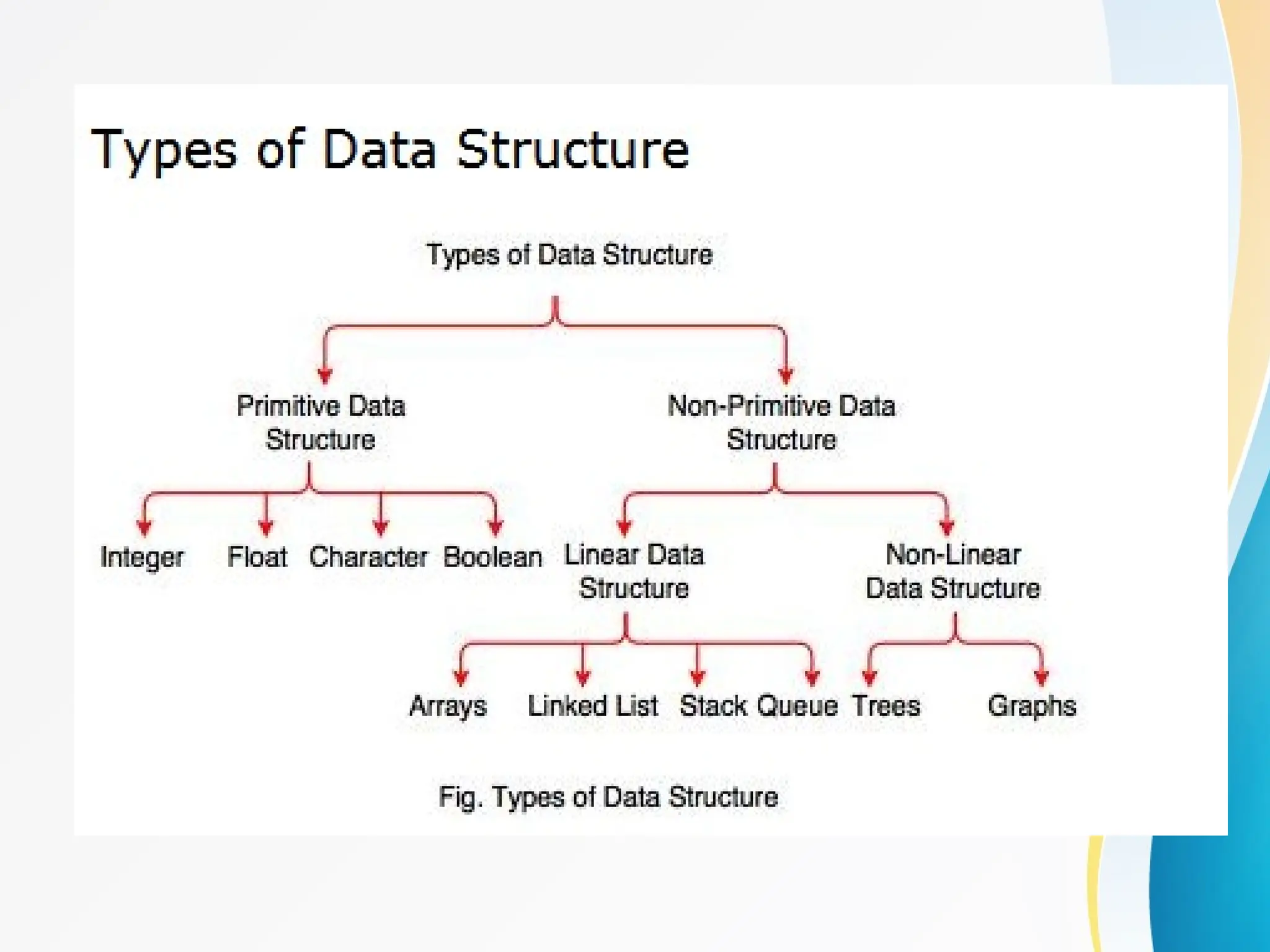
Concept of Problem Solving, Introduction to Algorithms, Characteristics of Algorithms, Introduction to Data Structure, Data Structure Classification (Linear and Non-linear, Static and Dynamic, Persistent and Ephemeral data structures), Time complexity and Space complexity, Asymptotic Notation - The Big-O, Omega and Theta notation, Algorithmic upper bounds, lower bounds, Best, Worst and Average case analysis of an Algorithm, Abstract Data Types (ADT)


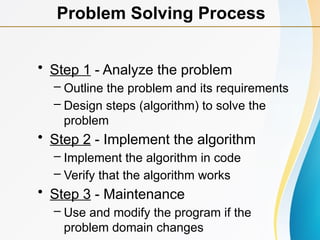
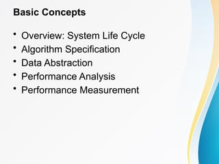

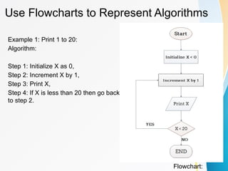
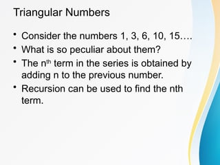
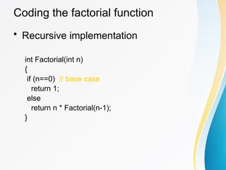
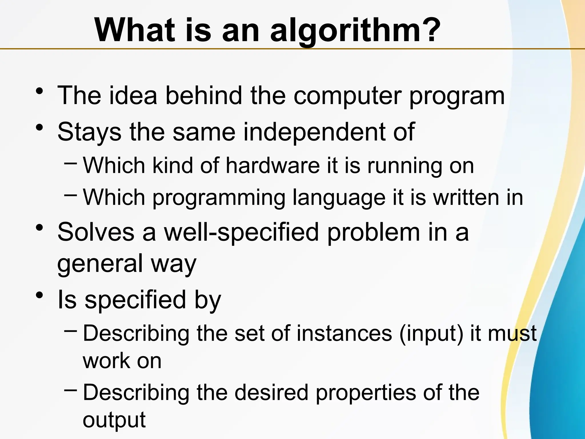
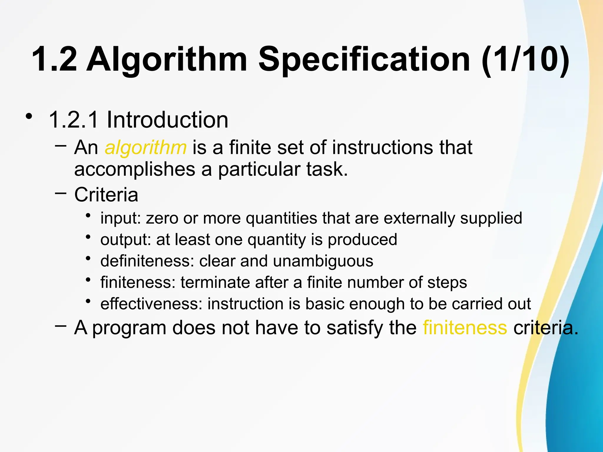
![1.2 Algorithm Specification (2/10)
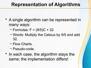
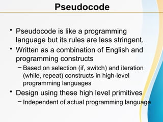
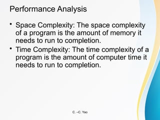
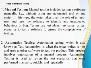
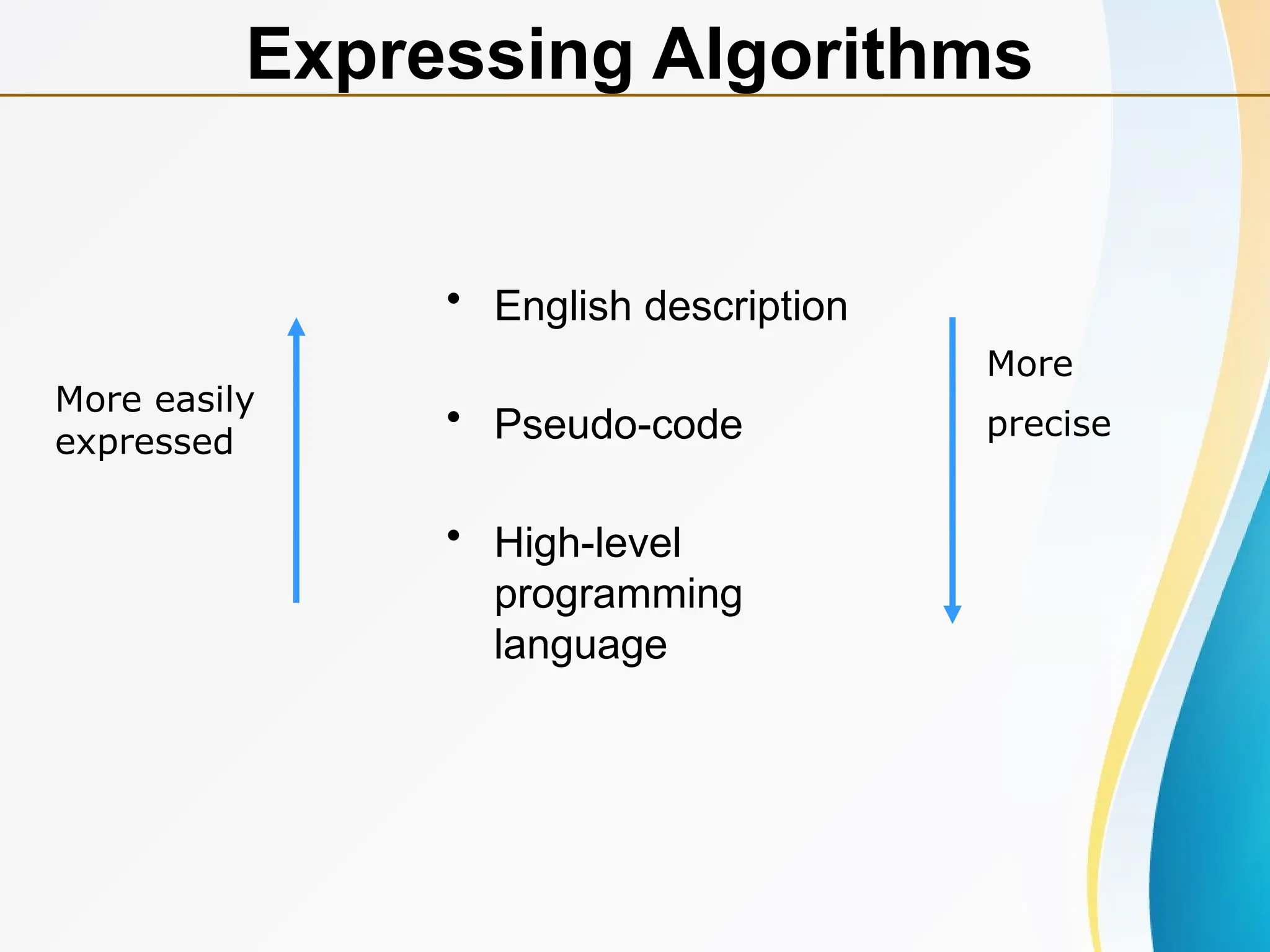
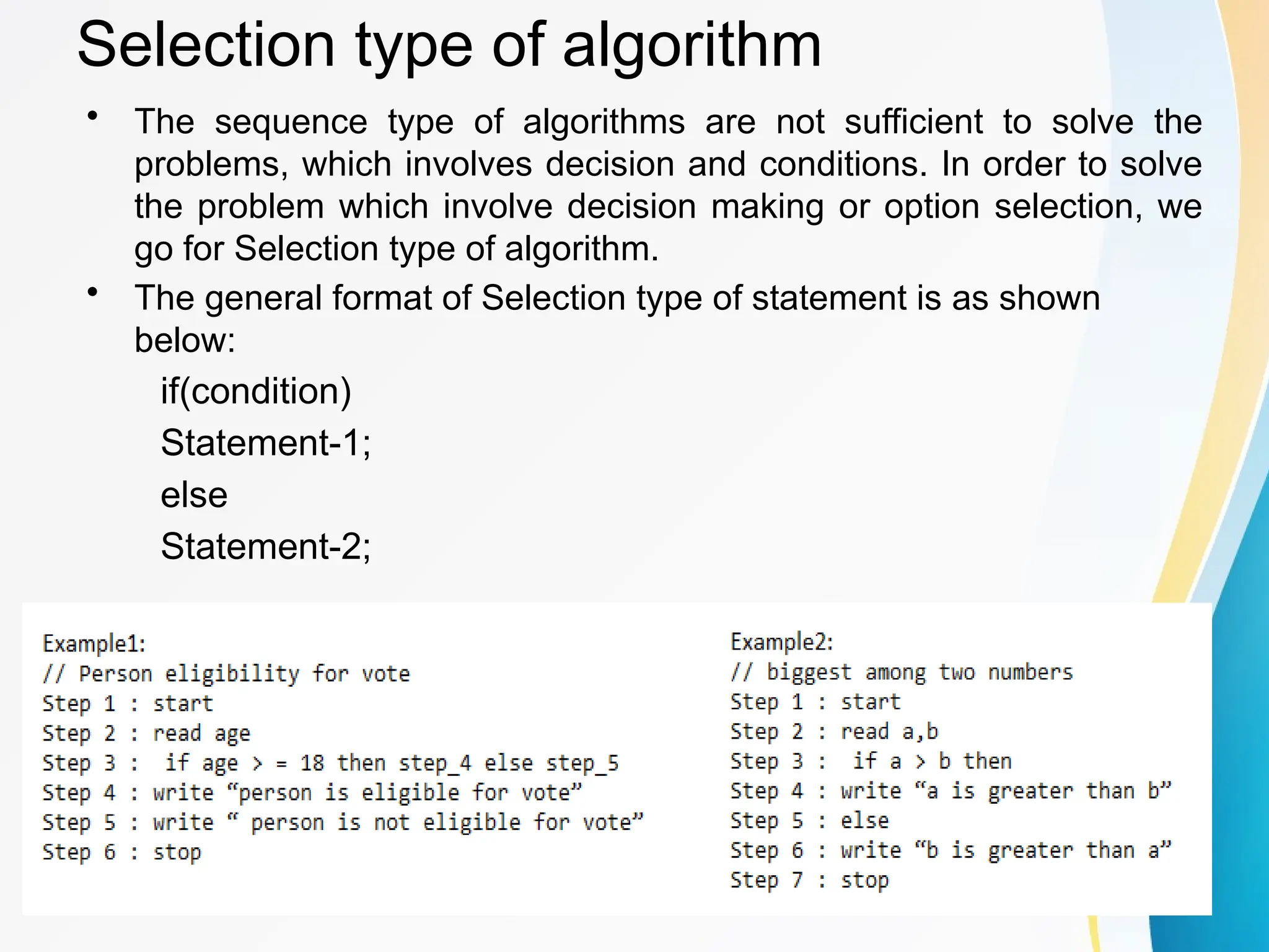
• Representation
– A natural language, like English or Chinese.
– A graphic, like flowcharts.
– A computer language, like C.
• Algorithms + Data structures =
Programs [Niklus Wirth]
• Sequential search vs. Binary search](https://image.slidesharecdn.com/datastructuresintroductiontoalgorithms-250503112821-7b6e2e04/85/Data-Structures_Introduction-to-algorithms-pptx-12-320.jpg)
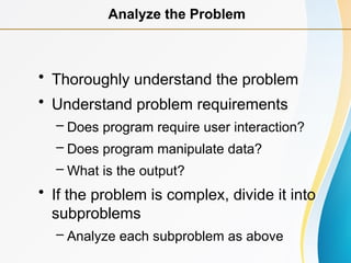
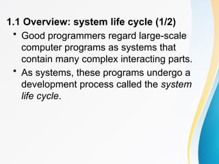
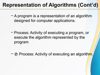
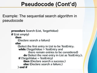
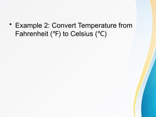
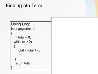
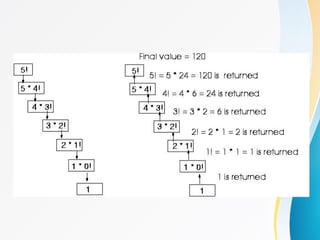
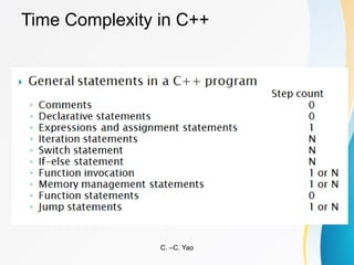
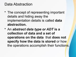
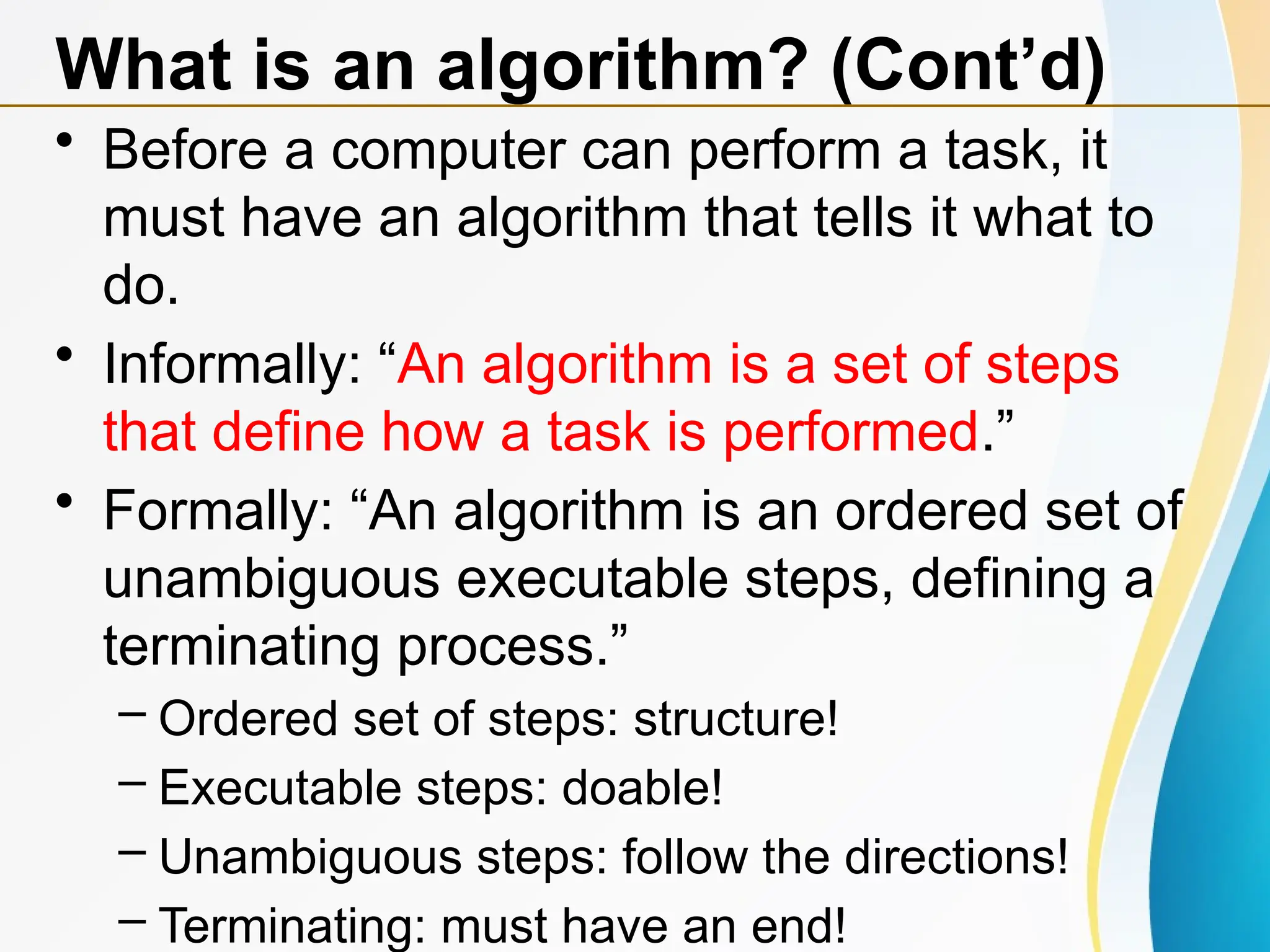
![• Example 1.1 [Selection sort]:
– From those integers that are currently unsorted, find the
smallest and place it next in the sorted list.
i [0] [1] [2] [3] [4]
- 30 10 50 40 20
0 10 30 50 40 20
1 10 20 40 50 30
2 10 20 30 40 50
3 10 20 30 40 50
1.2 Algorithm Specification (3/10)](https://image.slidesharecdn.com/datastructuresintroductiontoalgorithms-250503112821-7b6e2e04/85/Data-Structures_Introduction-to-algorithms-pptx-13-320.jpg)
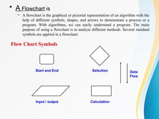
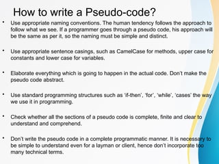


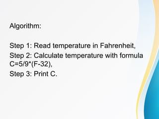


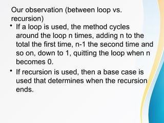
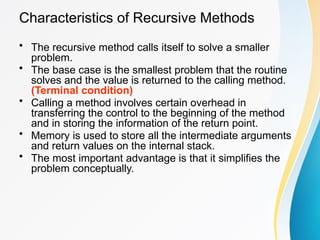


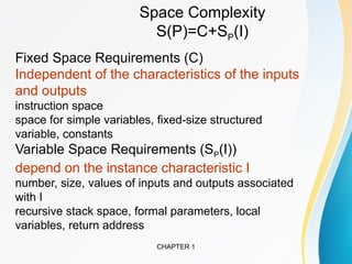


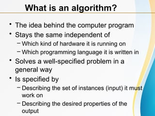
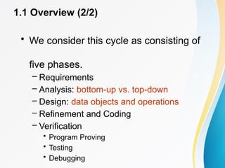
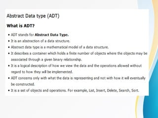
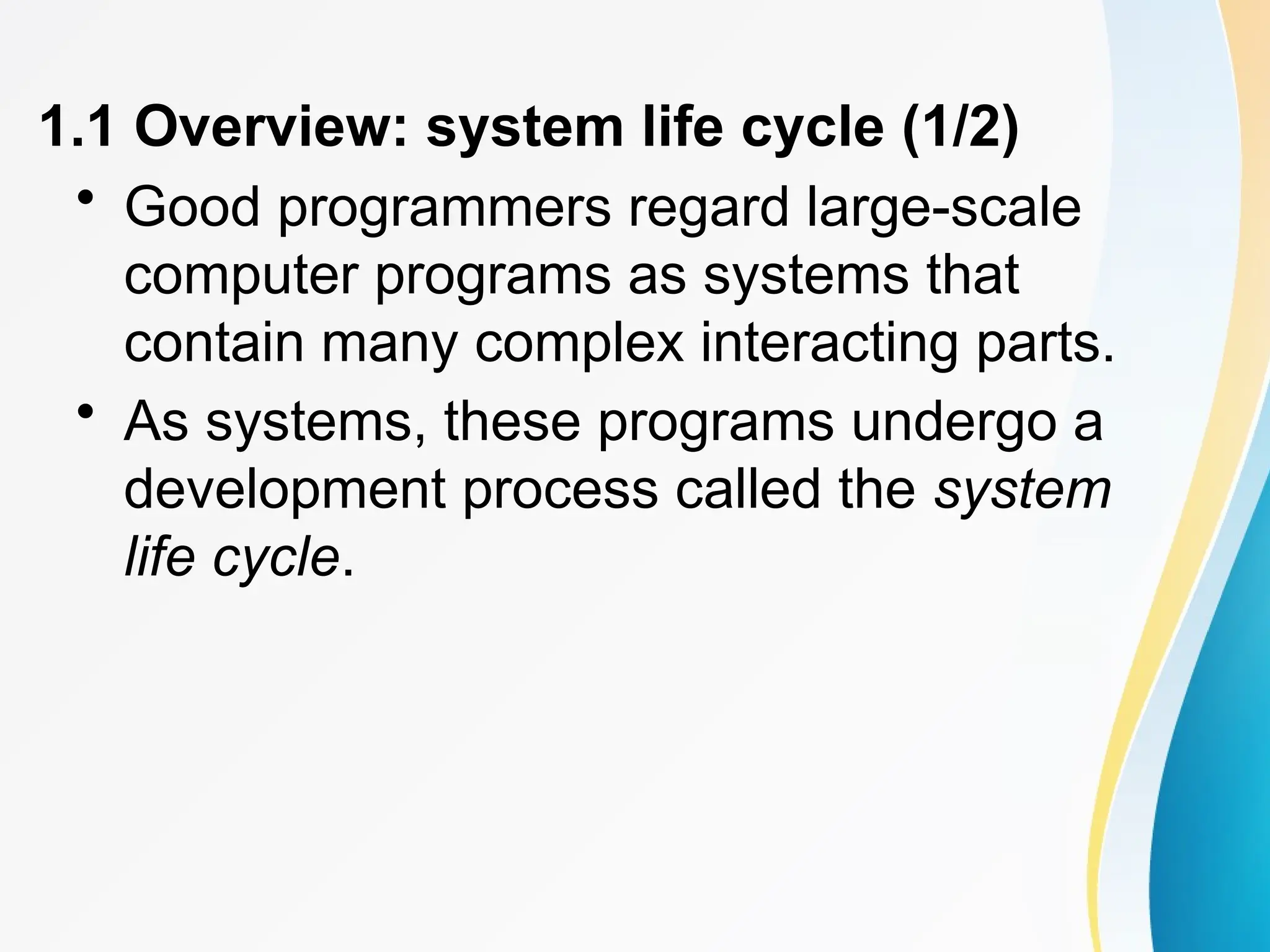
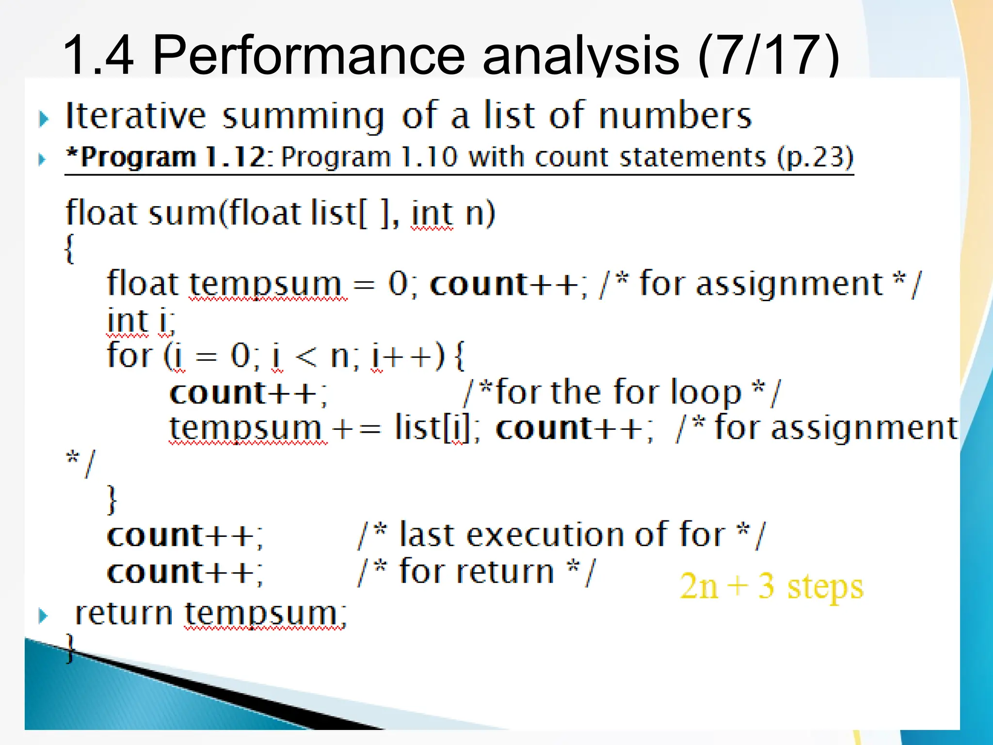
![• Tabular Method
• *Figure 1.2: Step count table for Program 1.10 (p.26)
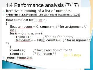
1.4 Performance analysis (8/17)
Statement s/e Frequency Total steps
float sum(float list[ ], int n)
{
float tempsum = 0;
int i;
for(i=0; i <n; i++)
tempsum += list[i];
return tempsum;
}
0 0 0
0 0 0
1 1 1
0 0 0
1 n+1 n+1
1 n n
1 1 1
0 0 0
Total 2n+3
steps/execution
Iterative function to sum a list of numbers](https://image.slidesharecdn.com/datastructuresintroductiontoalgorithms-250503112821-7b6e2e04/85/Data-Structures_Introduction-to-algorithms-pptx-70-320.jpg)
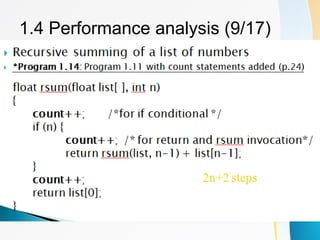
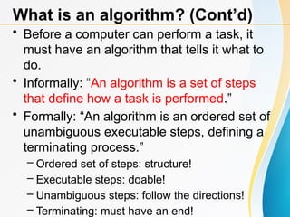
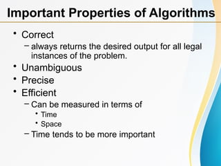
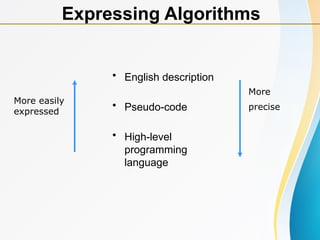
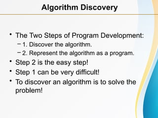
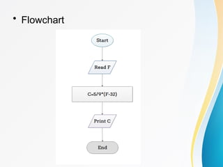
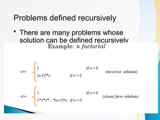
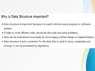
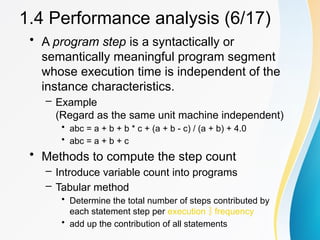
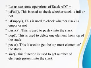
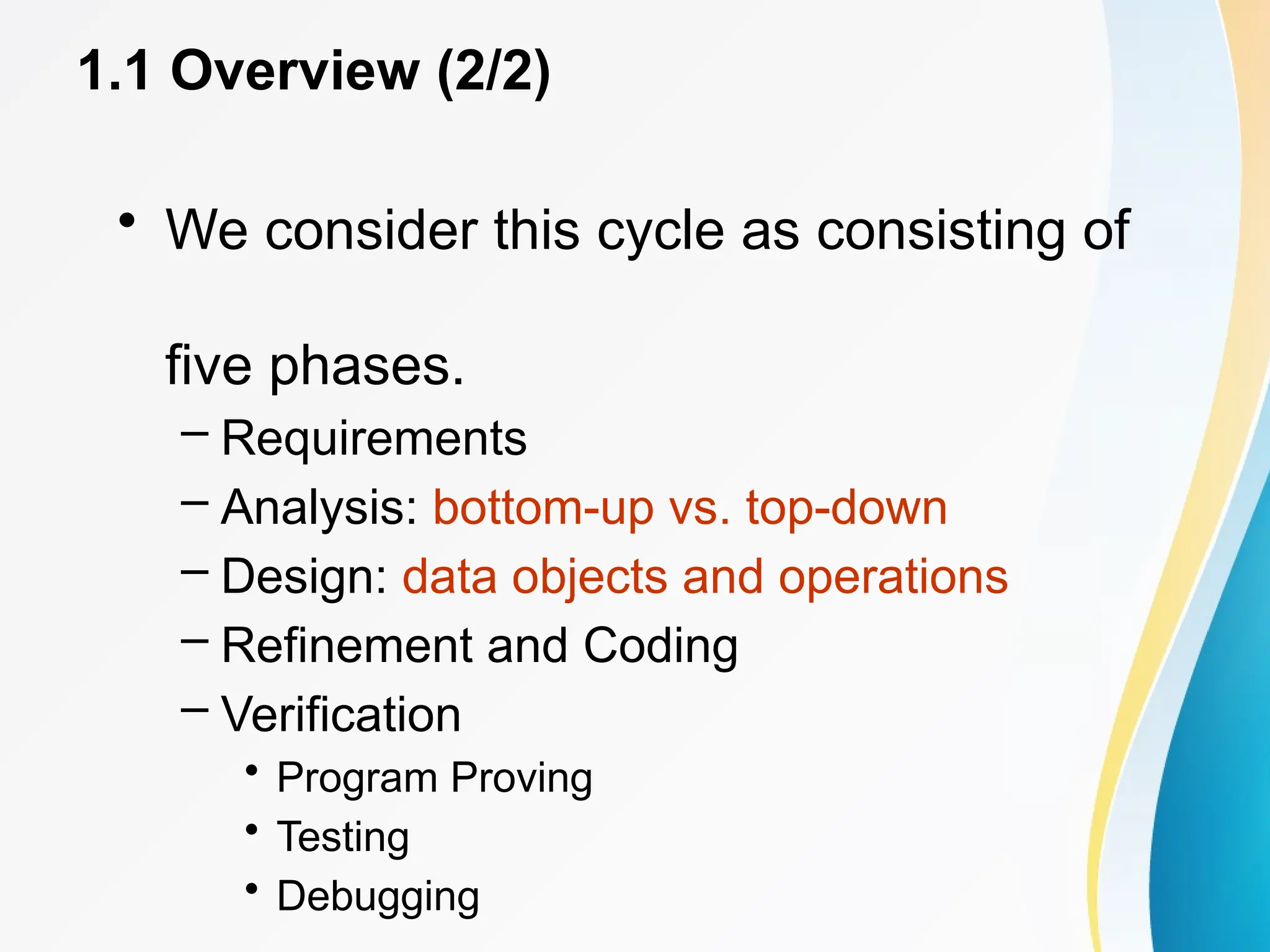
![• *Figure 1.3: Step count table for recursive summing function
(p.27)
1.4 Performance analysis (10/17)
Statement s/e Frequency Total steps
float rsum(float list[ ], int n)
{
if (n)
return rsum(list, n-1)+list[n-1];
return list[0];
}
0 0 0
0 0 0
1 n+1 n+1
1 n n
1 1 1
0 0 0
Total 2n+2](https://image.slidesharecdn.com/datastructuresintroductiontoalgorithms-250503112821-7b6e2e04/85/Data-Structures_Introduction-to-algorithms-pptx-72-320.jpg)


![1.2 Algorithm Specification (2/10)
• Representation
– A natural language, like English or Chinese.
– A graphic, like flowcharts.
– A computer language, like C.
• Algorithms + Data structures =
Programs [Niklus Wirth]
• Sequential search vs. Binary search](https://image.slidesharecdn.com/datastructuresintroductiontoalgorithms-250503112821-7b6e2e04/75/Data-Structures_Introduction-to-algorithms-pptx-12-2048.jpg)
![• Example 1.1 [Selection sort]:
– From those integers that are currently unsorted, find the
smallest and place it next in the sorted list.
i [0] [1] [2] [3] [4]
- 30 10 50 40 20
0 10 30 50 40 20
1 10 20 40 50 30
2 10 20 30 40 50
3 10 20 30 40 50
1.2 Algorithm Specification (3/10)](https://image.slidesharecdn.com/datastructuresintroductiontoalgorithms-250503112821-7b6e2e04/75/Data-Structures_Introduction-to-algorithms-pptx-13-2048.jpg)


![• Tabular Method
• *Figure 1.2: Step count table for Program 1.10 (p.26)
1.4 Performance analysis (8/17)
Statement s/e Frequency Total steps
float sum(float list[ ], int n)
{
float tempsum = 0;
int i;
for(i=0; i <n; i++)
tempsum += list[i];
return tempsum;
}
0 0 0
0 0 0
1 1 1
0 0 0
1 n+1 n+1
1 n n
1 1 1
0 0 0
Total 2n+3
steps/execution
Iterative function to sum a list of numbers](https://image.slidesharecdn.com/datastructuresintroductiontoalgorithms-250503112821-7b6e2e04/75/Data-Structures_Introduction-to-algorithms-pptx-70-2048.jpg)
![• *Figure 1.3: Step count table for recursive summing function
(p.27)
1.4 Performance analysis (10/17)
Statement s/e Frequency Total steps
float rsum(float list[ ], int n)
{
if (n)
return rsum(list, n-1)+list[n-1];
return list[0];
}
0 0 0
0 0 0
1 n+1 n+1
1 n n
1 1 1
0 0 0
Total 2n+2](https://image.slidesharecdn.com/datastructuresintroductiontoalgorithms-250503112821-7b6e2e04/75/Data-Structures_Introduction-to-algorithms-pptx-72-2048.jpg)