Download as PDF, PPTX

![What is Association Mining?
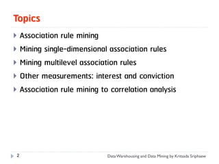
Association rule mining:
Finding frequent patterns, associations, correlations, or causal
structures among sets of items or objects in transaction
databases, relational databases, and other information
repositories.
Applications:
Basket data analysis, cross-marketing, catalog design,
clustering, classification, etc.
Ex.: Rule form: “Body Head [support, confidence]”
buys(x, “diapers*”) Consequent [support, confidence]”
“Antecedent buys(x, “beers”) [0.5%,60%]
major(x, “CS”)^takes(x, “DB”) grade(x, “A”) [1%, 75%]
3 Data Warehousing and Data Mining by Kritsada Sriphaew](https://image.slidesharecdn.com/dbm630-lecture05-120208002043-phpapp02/85/Dbm630-lecture05-3-320.jpg)
![Association Rule Mining: Types
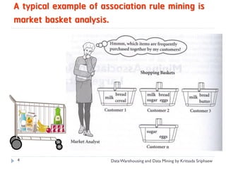
Boolean vs. quantitative associations (Based on the types of
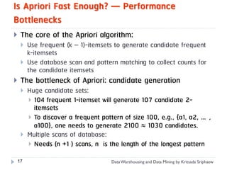
values handled) (Single vs. multiple Dim.)
SQLServer ^ DMBooks DBMiner [0.2%, 60%]
buys(x, “SQLServer”) ^ buys(x, “DMBook”)
buys(x, “DBMiner”) [0.2%, 60%]
age(x, “30..39”) ^ income(x, “42..48K”)
buys(x, “PC”) [1%, 75%]
Single level vs. multilevel analysis
What brands of beers are associated with what brands of diapers?
Various extensions
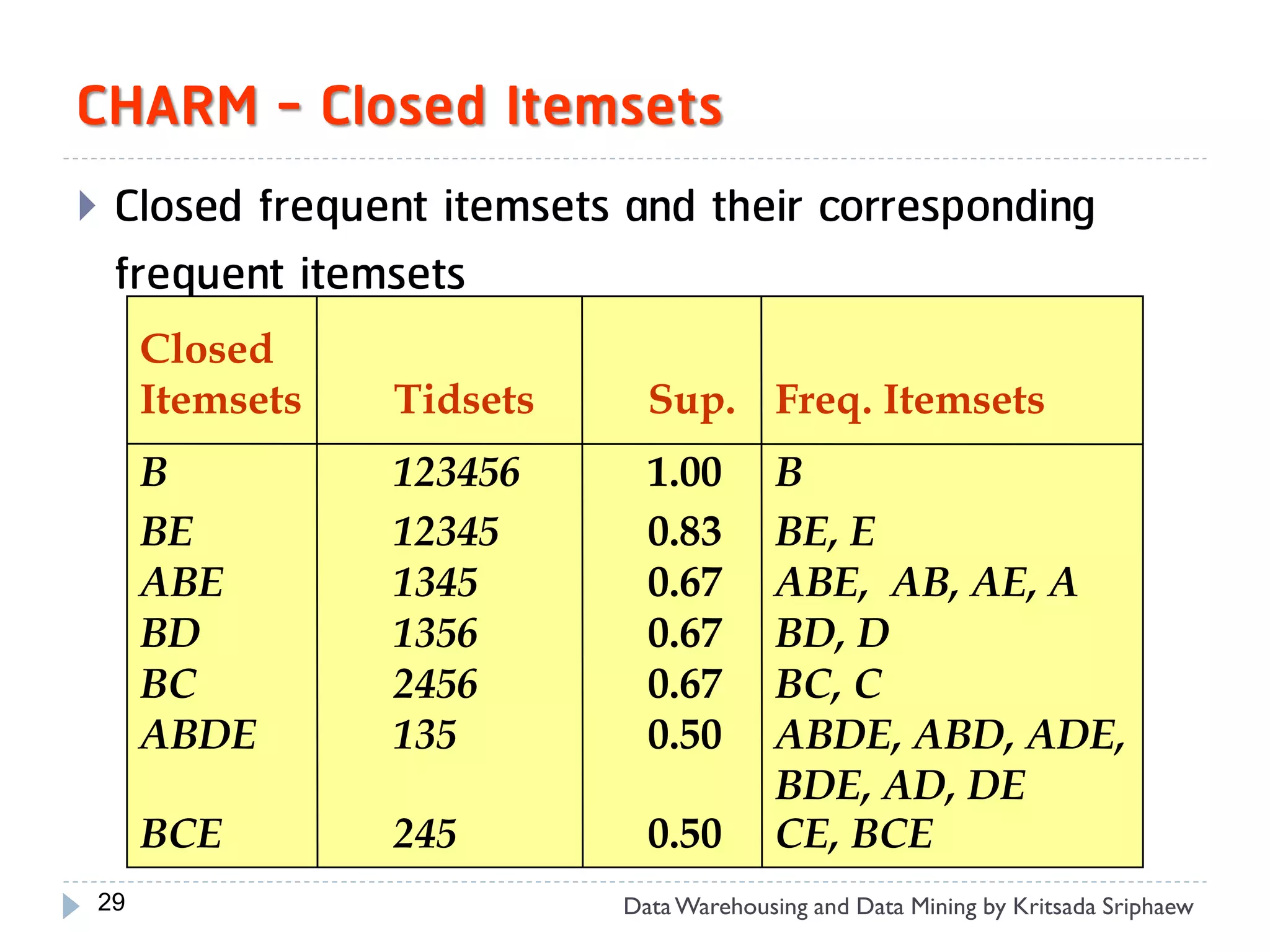
Maxpatterns and closed itemsets
8 Data Warehousing and Data Mining by Kritsada Sriphaew](https://image.slidesharecdn.com/dbm630-lecture05-120208002043-phpapp02/85/Dbm630-lecture05-8-320.jpg)

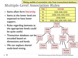
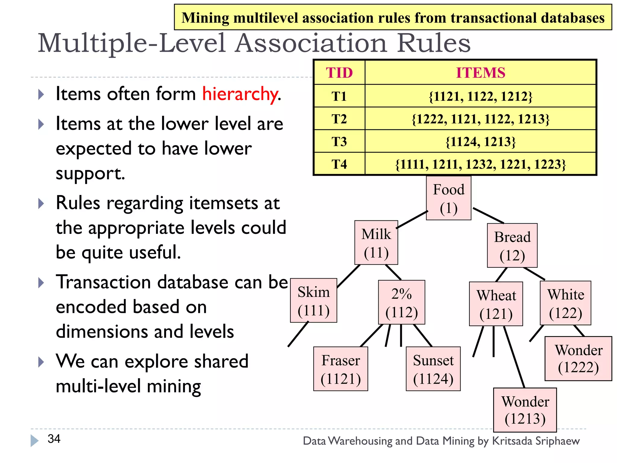
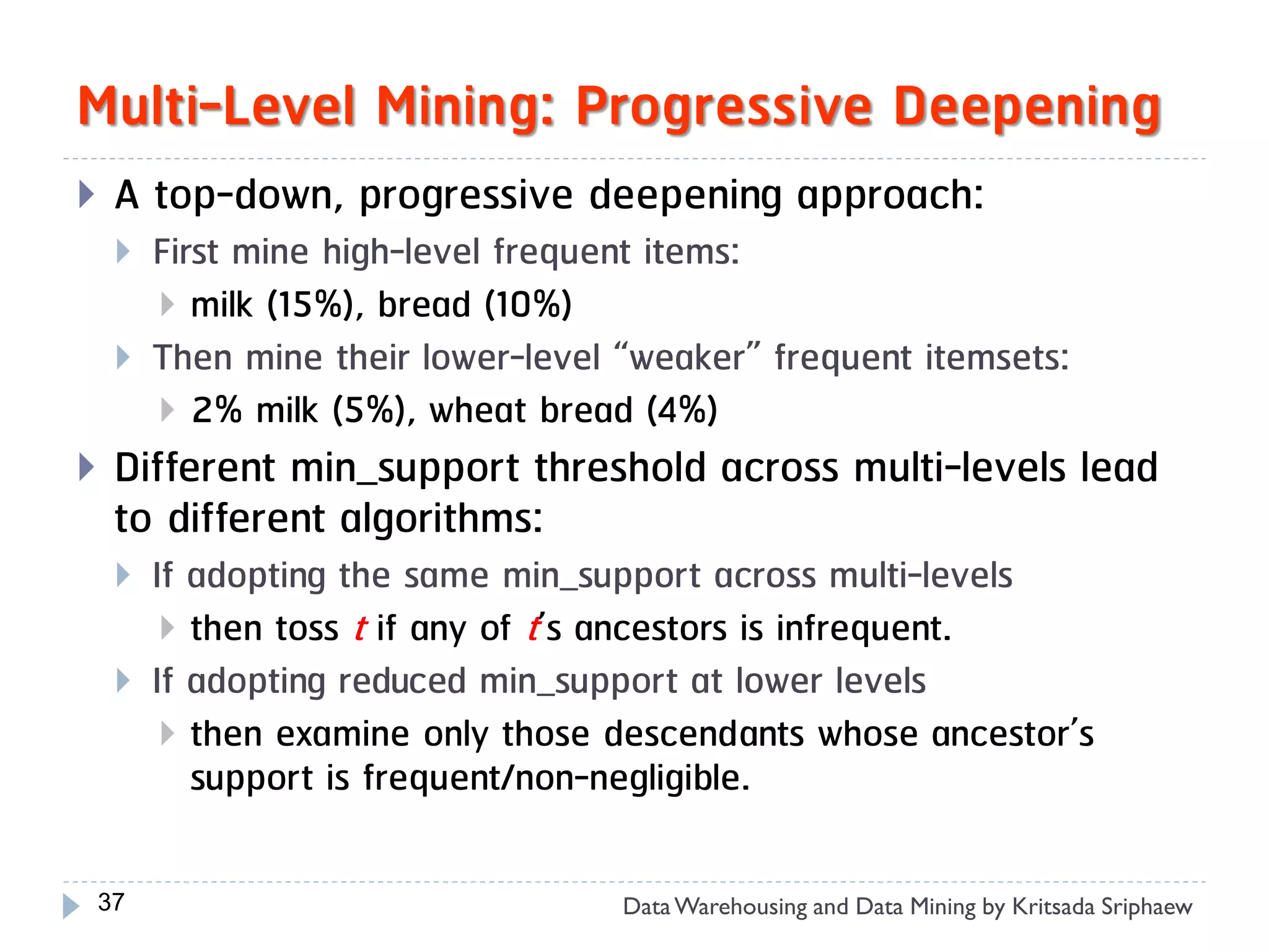
![Mining Multi-Level Associations
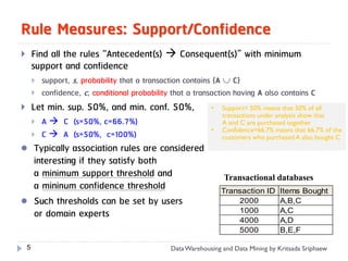
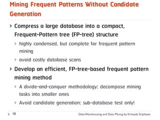
A top_down, progressive deepening approach:
First find high-level strong rules:
milk bread [20%, 60%]
Then find their lower-level “weaker” rules:
2% milk wheat bread [6%, 50%]
Variations at mining multiple-level association rules.
Level-crossed association rules:
2% milk Wonder wheat bread [3%, 60%]
Association rules with multiple, alternative hierarchies:
2% milk Wonder bread [8%, 72%]
35 Data Warehousing and Data Mining by Kritsada Sriphaew](https://image.slidesharecdn.com/dbm630-lecture05-120208002043-phpapp02/85/Dbm630-lecture05-35-320.jpg)
![Multi-level Association: Redundancy Filtering
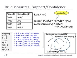
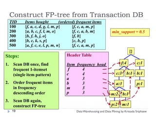
Some rules may be redundant due to “ancestor”
relationships between items.
Example
milk wheat bread [s=8%, c=70%]
2% milk wheat bread [s=2%, c=72%]
We say the first rule is an ancestor of the second
rule.
A rule is redundant if its support is close to the
“expected” value, based on the rule’s ancestor.
36 Data Warehousing and Data Mining by Kritsada Sriphaew](https://image.slidesharecdn.com/dbm630-lecture05-120208002043-phpapp02/85/Dbm630-lecture05-36-320.jpg)

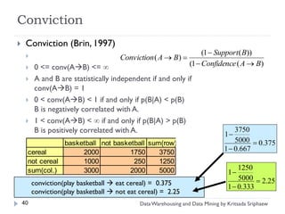
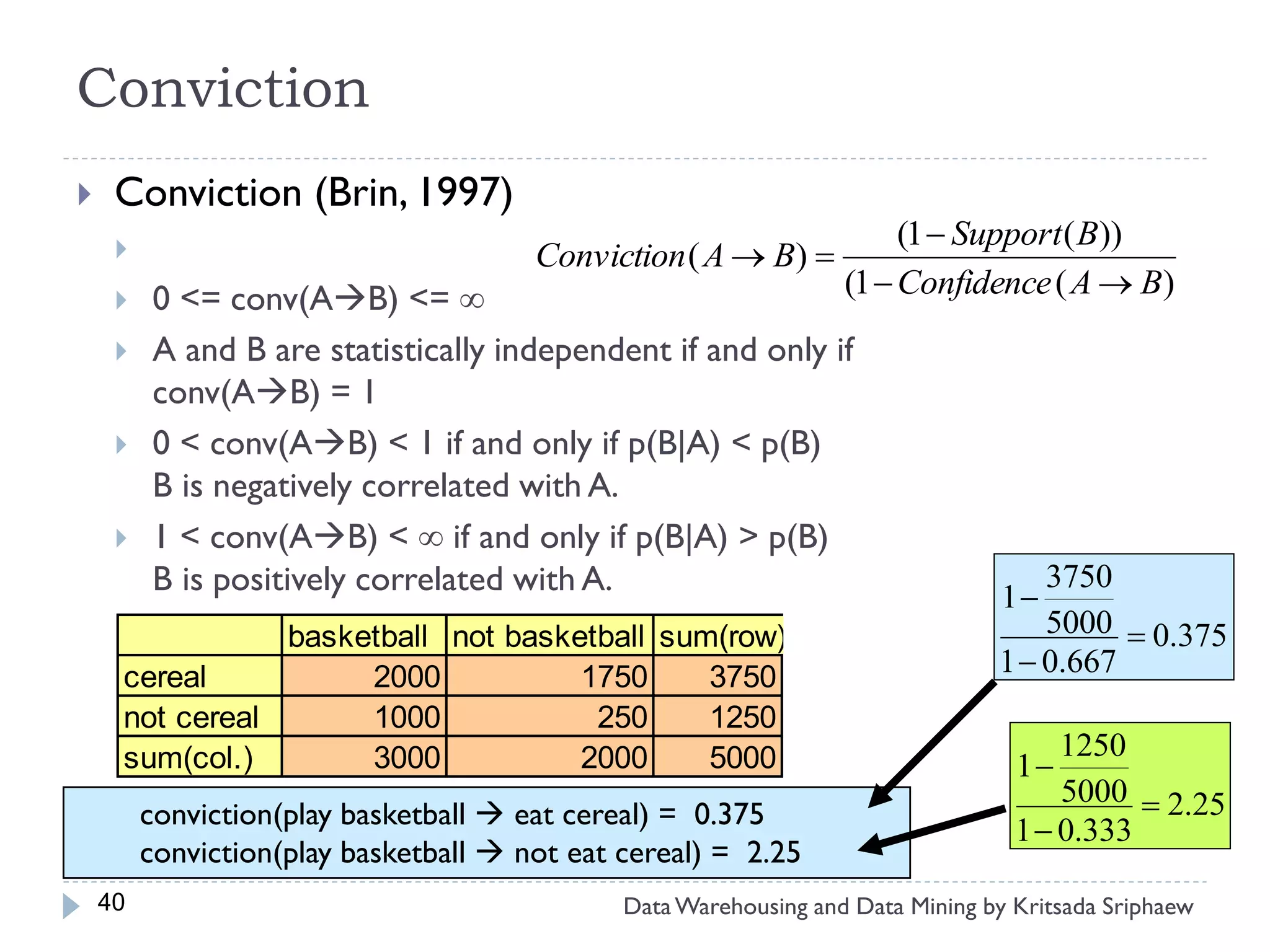
![Problem of Confidence
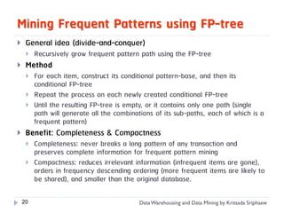
Example: (Aggarwal & Yu, PODS98)
Among 5000 students
3000 play basketball
3750 eat cereal
2000 both play basket ball and eat cereal
play basketball eat cereal [40%, 66.7%] is misleading because the overall
percentage of students eating cereal is 75% which is higher than 66.7%.
play basketball not eat cereal [20%, 33.3%] is far more accurate, although
with lower support and confidence
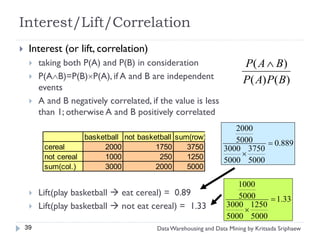
basketball not basketball sum(row)
cereal 2000 1750 3750
not cereal 1000 250 1250
sum(col.) 3000 2000 5000
38 Data Warehousing and Data Mining by Kritsada Sriphaew](https://image.slidesharecdn.com/dbm630-lecture05-120208002043-phpapp02/85/Dbm630-lecture05-38-320.jpg)
![From Association Mining to Correlation Analysis
Ex. Strong rules are not necessarily interesting
Of 10000 transactions
• 6000 customer transactions include computer games
• 7500 customer transactions include videos
• 4000 customer transactions include both computer game and video
• Suppose that data mining program for
videos games
discovering association rules is run on
the data, using min_sup of 30% and
min_conf. of 60%
• The following association rule is
discovered:
4,000
buys(X, “computer games”) buys(X, “videos”)
[s=40%, c=66%]
41
=4000/10000 =4000/6000](https://image.slidesharecdn.com/dbm630-lecture05-120208002043-phpapp02/85/Dbm630-lecture05-41-320.jpg)
![A misleading “strong” association rule
buys(X, “computer games”) buys(X, “videos”)
[support=40%, confidence=66%]
This rule is misleading because the probability of purchasing video is
75% (>66%)
In fact, computer games and videos are negatively associated because
the purchase of one of these items actually decreases the likelihood of
purchasing the other. Therefore, we could easily make unwise business
decisions based on this rule
42
Data Warehousing and Data Mining by Kritsada Sriphaew](https://image.slidesharecdn.com/dbm630-lecture05-120208002043-phpapp02/85/Dbm630-lecture05-42-320.jpg)
![From Association Analysis to Correlation
Analysis
To help filter out misleading “strong” association
Correlation rules
A B [support, confidence, correlation]
Lift is a simple correlation measure that is given as follows
The occurrence of itemset A is independent of the occurrence of itemset B if
P(AB) = P(A)P(B);
Otherwise, itemset A and B are dependent and correlated
lift(A,B) = P(AB) / P(A)P(B) = P(B|A) / P(B) = conf(AB) / sup(B)
If lift(A,B) < 1, then the occurrence of A is negatively correlated with the
occurrence of B
If lift(A,B) > 1, then A and B is positively correlated, meaning that the occurrence
of one implies the occurrence of the other.
43
Data Warehousing and Data Mining by Kritsada Sriphaew](https://image.slidesharecdn.com/dbm630-lecture05-120208002043-phpapp02/85/Dbm630-lecture05-43-320.jpg)
![From Association Analysis to Correlation
Analysis (Cont.)
Ex. Correlation analysis using lift
buys(X, “computer games”) buys(X, “videos”)
[support=40%, confidence=66%]
The lift of this rule is
P{game,video} / (P{game} × P{video}) = 0.40/(0.6 ×0.75) = 0.89
There is a negative correlation between the occurrence of {game} and {video}
Ex. Is this following rule misleading?
Buy walnuts Buy milk [1%, 80%]”
if 85% of customers buy milk
44
Data Warehousing and Data Mining by Kritsada Sriphaew](https://image.slidesharecdn.com/dbm630-lecture05-120208002043-phpapp02/85/Dbm630-lecture05-44-320.jpg)
![What is Association Mining?
Association rule mining:
Finding frequent patterns, associations, correlations, or causal
structures among sets of items or objects in transaction
databases, relational databases, and other information
repositories.
Applications:
Basket data analysis, cross-marketing, catalog design,
clustering, classification, etc.
Ex.: Rule form: “Body Head [support, confidence]”
buys(x, “diapers*”) Consequent [support, confidence]”
“Antecedent buys(x, “beers”) [0.5%,60%]
major(x, “CS”)^takes(x, “DB”) grade(x, “A”) [1%, 75%]
3 Data Warehousing and Data Mining by Kritsada Sriphaew](https://image.slidesharecdn.com/dbm630-lecture05-120208002043-phpapp02/75/Dbm630-lecture05-3-2048.jpg)

![Association Rule Mining: Types
Boolean vs. quantitative associations (Based on the types of
values handled) (Single vs. multiple Dim.)
SQLServer ^ DMBooks DBMiner [0.2%, 60%]
buys(x, “SQLServer”) ^ buys(x, “DMBook”)
buys(x, “DBMiner”) [0.2%, 60%]
age(x, “30..39”) ^ income(x, “42..48K”)
buys(x, “PC”) [1%, 75%]
Single level vs. multilevel analysis
What brands of beers are associated with what brands of diapers?
Various extensions
Maxpatterns and closed itemsets
8 Data Warehousing and Data Mining by Kritsada Sriphaew](https://image.slidesharecdn.com/dbm630-lecture05-120208002043-phpapp02/75/Dbm630-lecture05-8-2048.jpg)


![Mining Multi-Level Associations
A top_down, progressive deepening approach:
First find high-level strong rules:
milk bread [20%, 60%]
Then find their lower-level “weaker” rules:
2% milk wheat bread [6%, 50%]
Variations at mining multiple-level association rules.
Level-crossed association rules:
2% milk Wonder wheat bread [3%, 60%]
Association rules with multiple, alternative hierarchies:
2% milk Wonder bread [8%, 72%]
35 Data Warehousing and Data Mining by Kritsada Sriphaew](https://image.slidesharecdn.com/dbm630-lecture05-120208002043-phpapp02/75/Dbm630-lecture05-35-2048.jpg)
![Multi-level Association: Redundancy Filtering
Some rules may be redundant due to “ancestor”
relationships between items.
Example
milk wheat bread [s=8%, c=70%]
2% milk wheat bread [s=2%, c=72%]
We say the first rule is an ancestor of the second
rule.
A rule is redundant if its support is close to the
“expected” value, based on the rule’s ancestor.
36 Data Warehousing and Data Mining by Kritsada Sriphaew](https://image.slidesharecdn.com/dbm630-lecture05-120208002043-phpapp02/75/Dbm630-lecture05-36-2048.jpg)
![Problem of Confidence
Example: (Aggarwal & Yu, PODS98)
Among 5000 students
3000 play basketball
3750 eat cereal
2000 both play basket ball and eat cereal
play basketball eat cereal [40%, 66.7%] is misleading because the overall
percentage of students eating cereal is 75% which is higher than 66.7%.
play basketball not eat cereal [20%, 33.3%] is far more accurate, although
with lower support and confidence
basketball not basketball sum(row)
cereal 2000 1750 3750
not cereal 1000 250 1250
sum(col.) 3000 2000 5000
38 Data Warehousing and Data Mining by Kritsada Sriphaew](https://image.slidesharecdn.com/dbm630-lecture05-120208002043-phpapp02/75/Dbm630-lecture05-38-2048.jpg)

![From Association Mining to Correlation Analysis
Ex. Strong rules are not necessarily interesting
Of 10000 transactions
• 6000 customer transactions include computer games
• 7500 customer transactions include videos
• 4000 customer transactions include both computer game and video
• Suppose that data mining program for
videos games
discovering association rules is run on
the data, using min_sup of 30% and
min_conf. of 60%
• The following association rule is
discovered:
4,000
buys(X, “computer games”) buys(X, “videos”)
[s=40%, c=66%]
41
=4000/10000 =4000/6000](https://image.slidesharecdn.com/dbm630-lecture05-120208002043-phpapp02/75/Dbm630-lecture05-41-2048.jpg)
![A misleading “strong” association rule
buys(X, “computer games”) buys(X, “videos”)
[support=40%, confidence=66%]
This rule is misleading because the probability of purchasing video is
75% (>66%)
In fact, computer games and videos are negatively associated because
the purchase of one of these items actually decreases the likelihood of
purchasing the other. Therefore, we could easily make unwise business
decisions based on this rule
42
Data Warehousing and Data Mining by Kritsada Sriphaew](https://image.slidesharecdn.com/dbm630-lecture05-120208002043-phpapp02/75/Dbm630-lecture05-42-2048.jpg)
![From Association Analysis to Correlation
Analysis
To help filter out misleading “strong” association
Correlation rules
A B [support, confidence, correlation]
Lift is a simple correlation measure that is given as follows
The occurrence of itemset A is independent of the occurrence of itemset B if
P(AB) = P(A)P(B);
Otherwise, itemset A and B are dependent and correlated
lift(A,B) = P(AB) / P(A)P(B) = P(B|A) / P(B) = conf(AB) / sup(B)
If lift(A,B) < 1, then the occurrence of A is negatively correlated with the
occurrence of B
If lift(A,B) > 1, then A and B is positively correlated, meaning that the occurrence
of one implies the occurrence of the other.
43
Data Warehousing and Data Mining by Kritsada Sriphaew](https://image.slidesharecdn.com/dbm630-lecture05-120208002043-phpapp02/75/Dbm630-lecture05-43-2048.jpg)
![From Association Analysis to Correlation
Analysis (Cont.)
Ex. Correlation analysis using lift
buys(X, “computer games”) buys(X, “videos”)
[support=40%, confidence=66%]
The lift of this rule is
P{game,video} / (P{game} × P{video}) = 0.40/(0.6 ×0.75) = 0.89
There is a negative correlation between the occurrence of {game} and {video}
Ex. Is this following rule misleading?
Buy walnuts Buy milk [1%, 80%]”
if 85% of customers buy milk
44
Data Warehousing and Data Mining by Kritsada Sriphaew](https://image.slidesharecdn.com/dbm630-lecture05-120208002043-phpapp02/75/Dbm630-lecture05-44-2048.jpg)


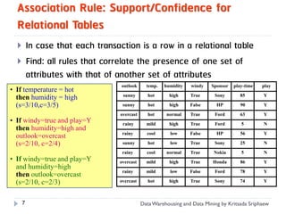
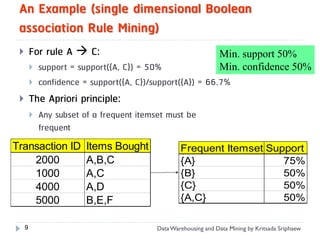
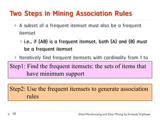
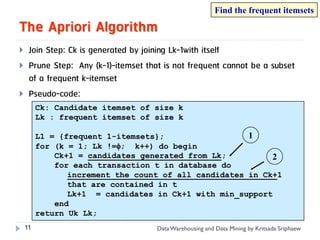
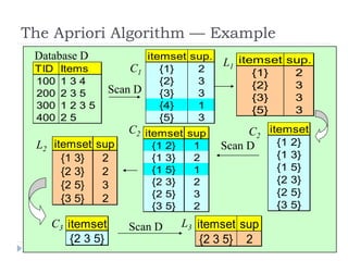
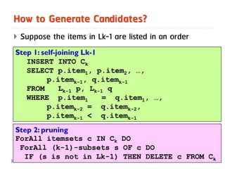
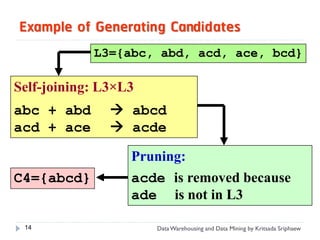
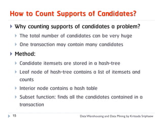
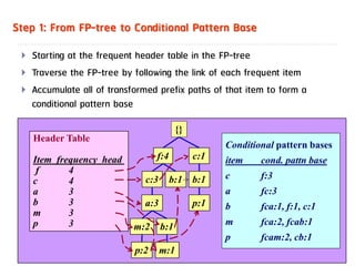
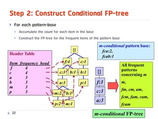
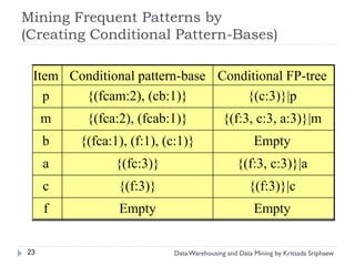
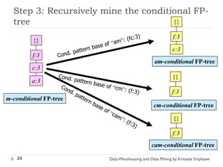
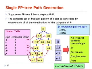
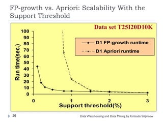
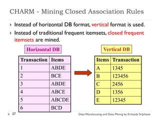
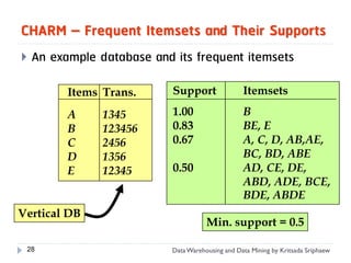
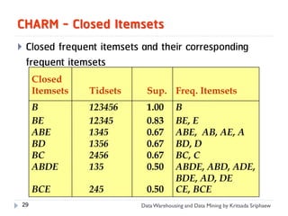
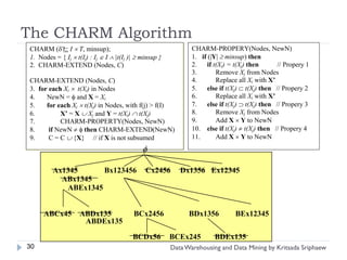
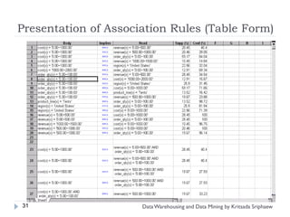
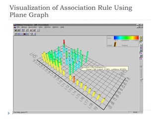
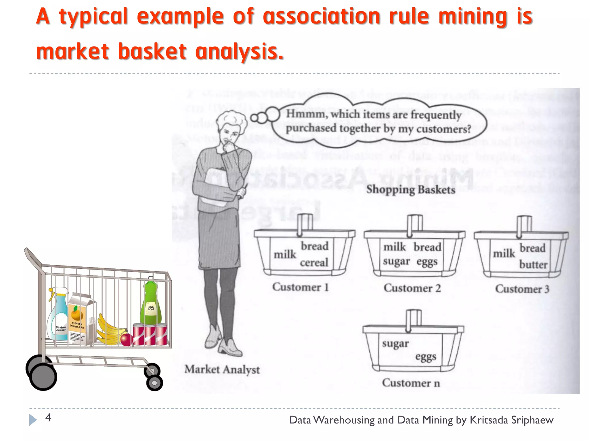
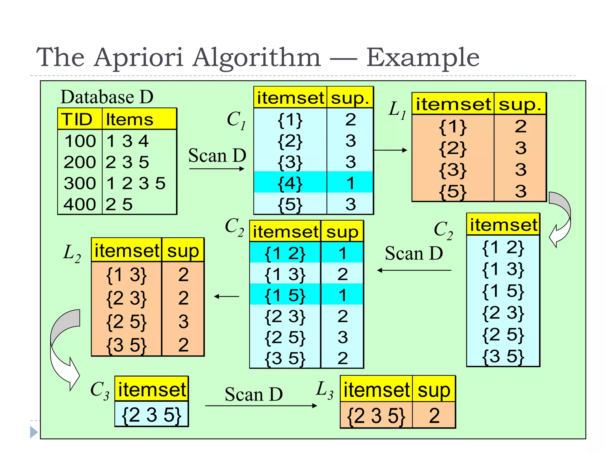
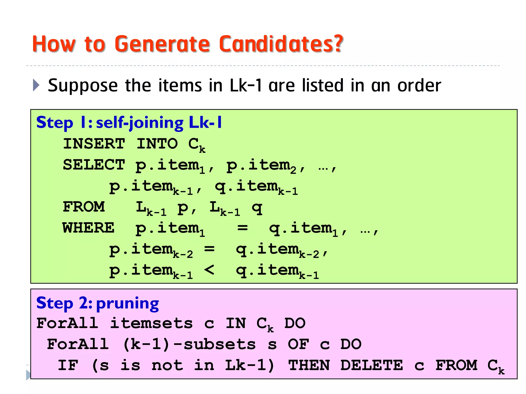
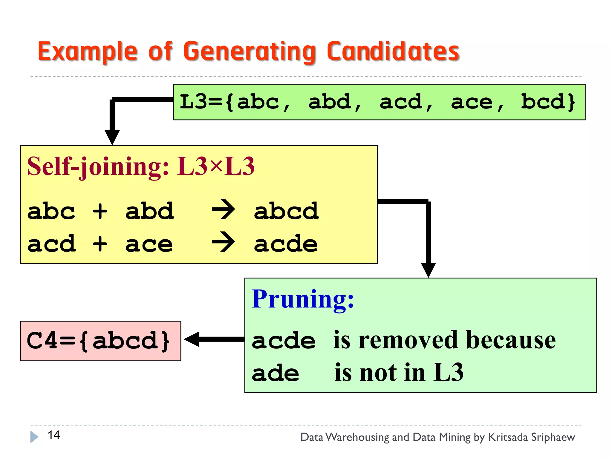
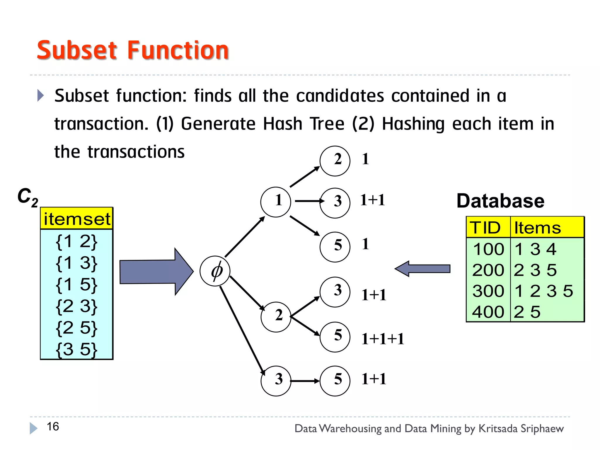
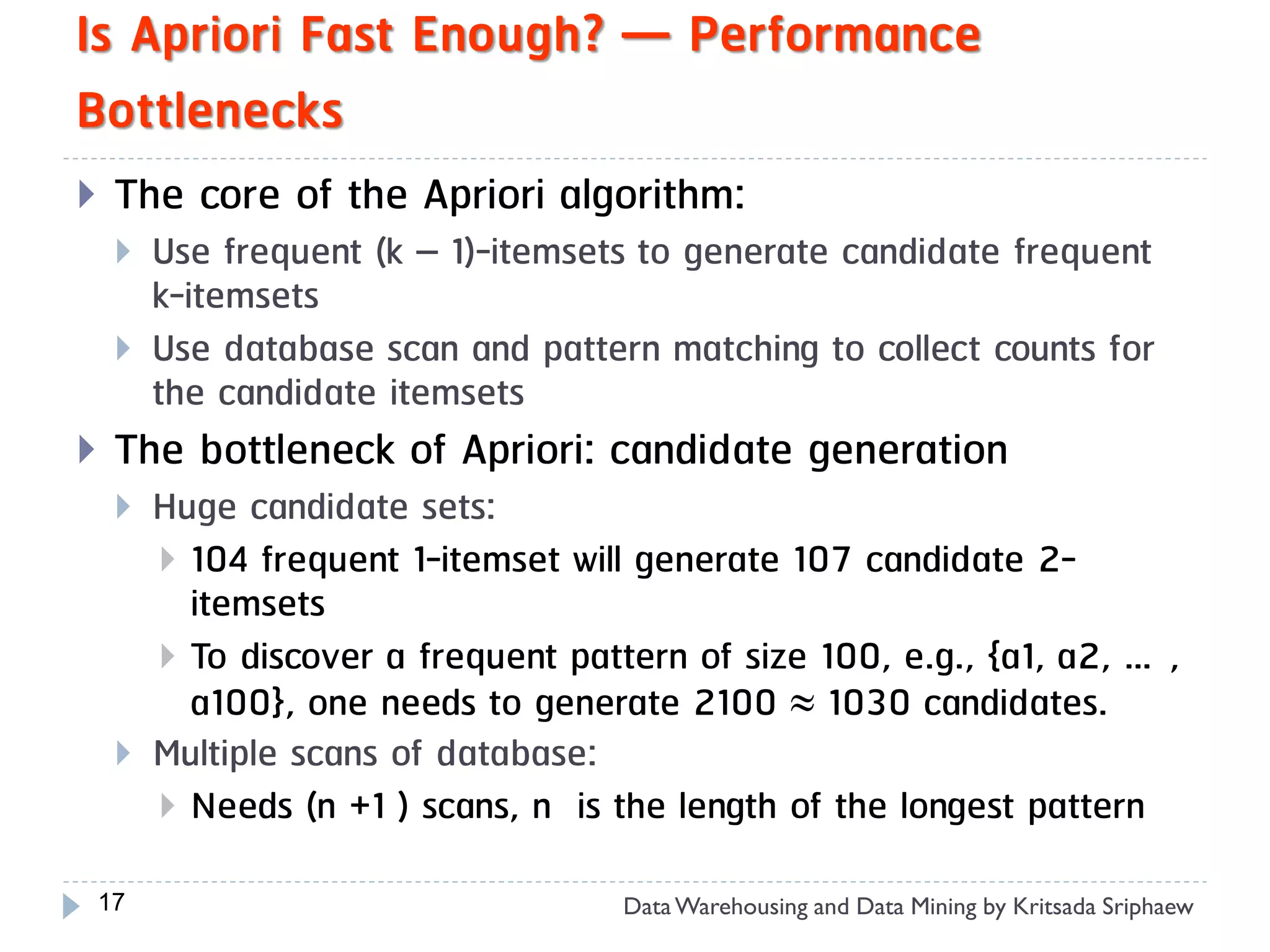
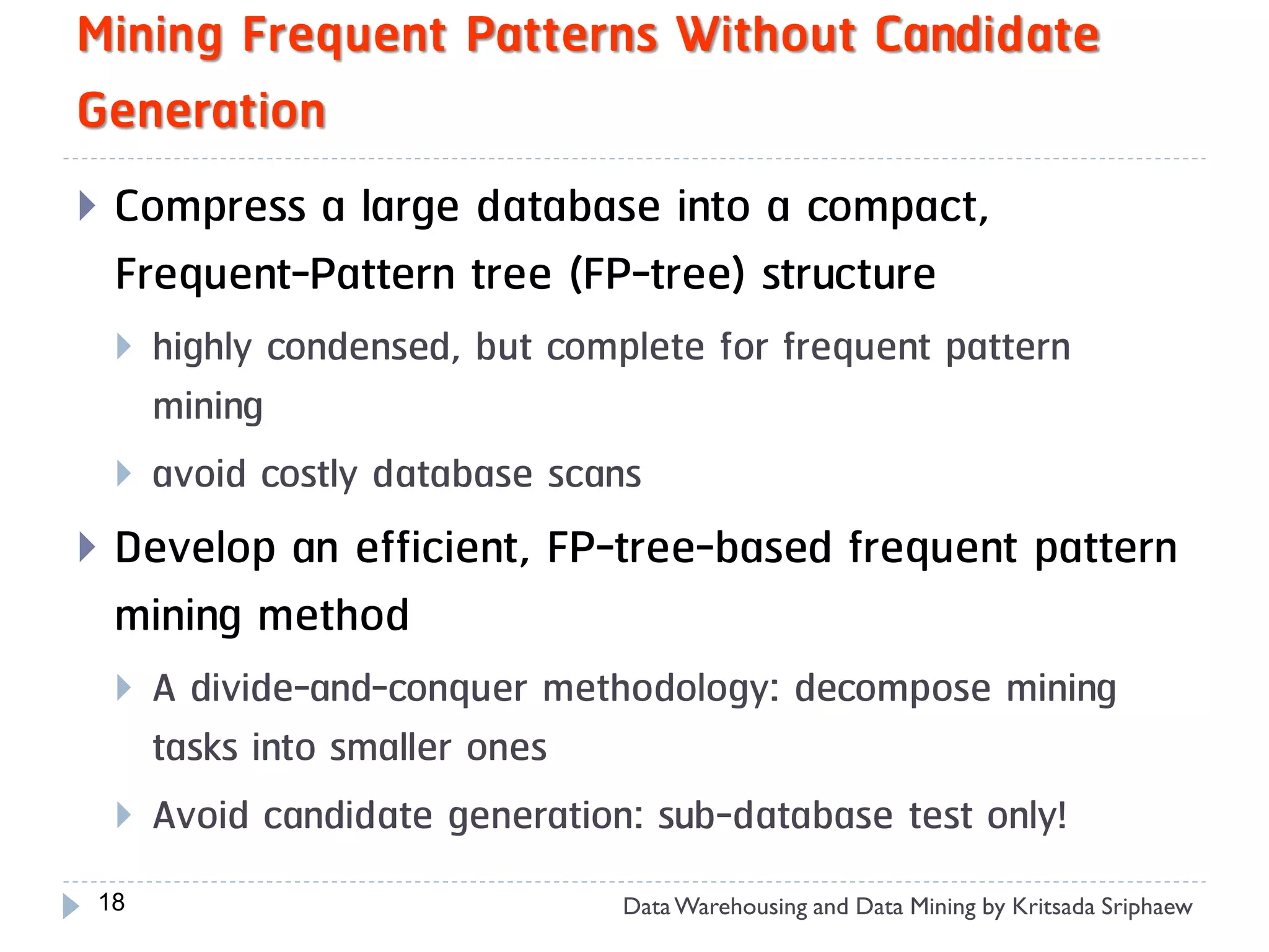
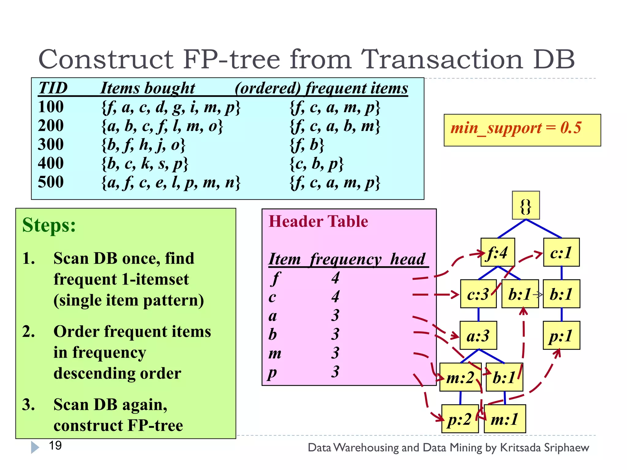
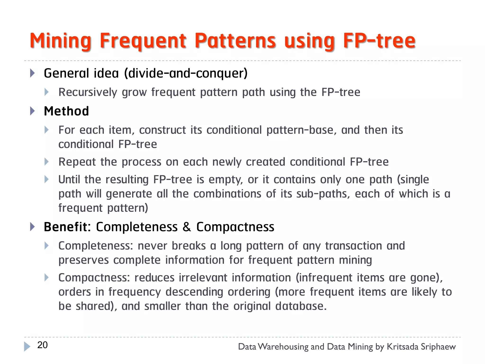
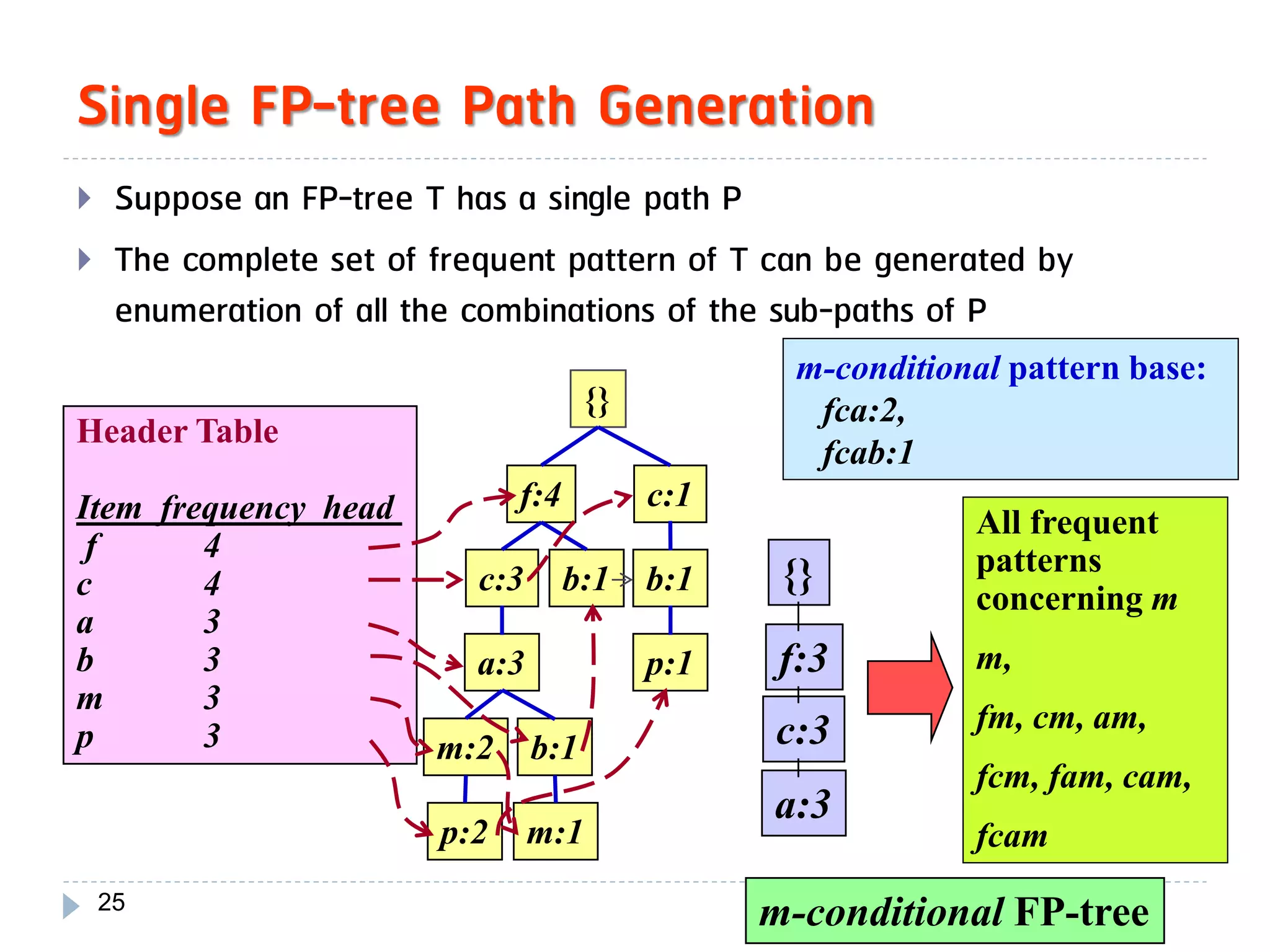
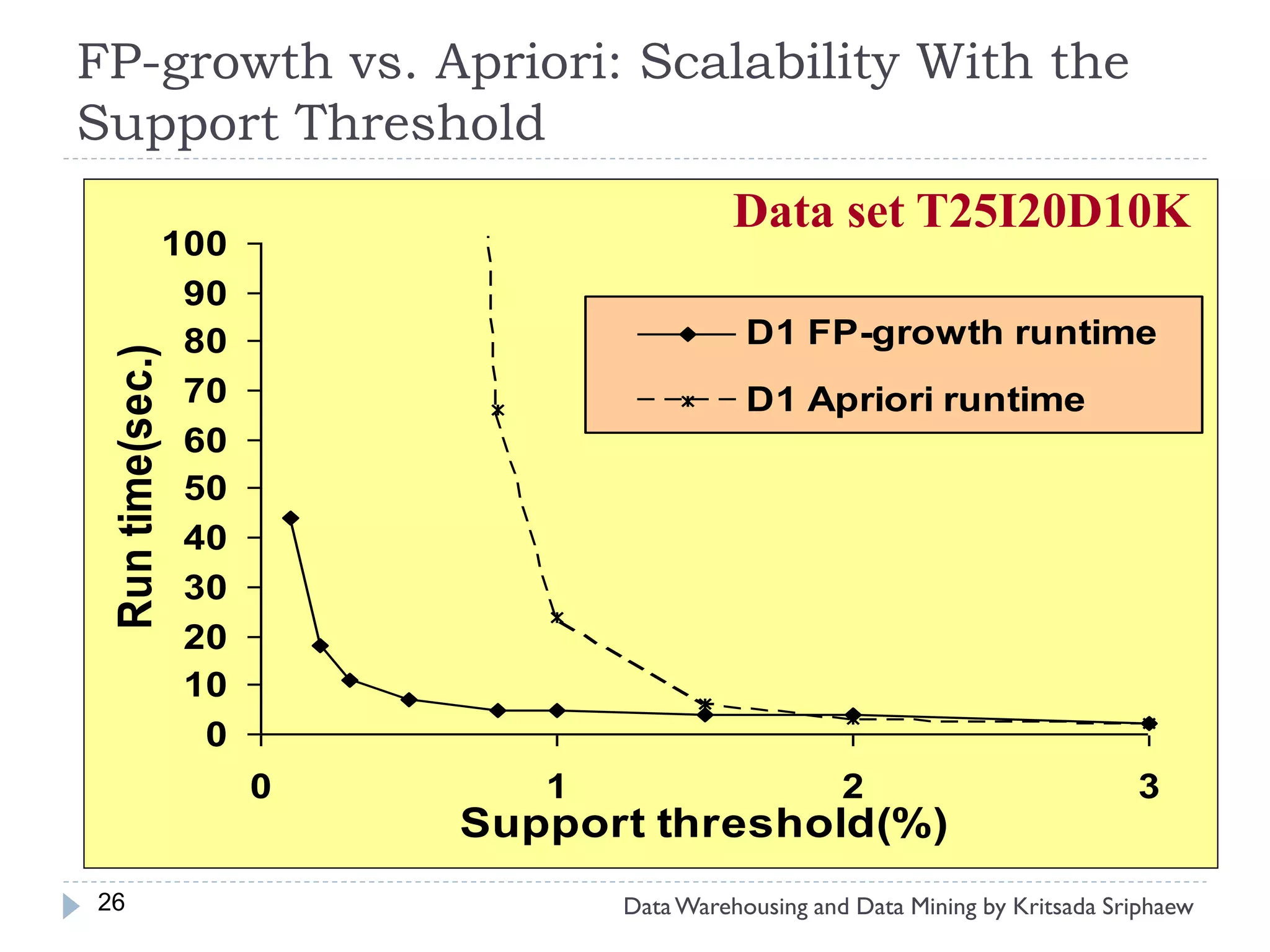
This document provides a summary of lecture 5 on association rule mining. It discusses topics like association rule mining, mining single and multilevel association rules, measurements like support and confidence. It provides examples of mining association rules from transactional databases and relational tables. It describes the Apriori algorithm for mining frequent itemsets and generating association rules. It also discusses techniques like FP-tree for overcoming performance issues of Apriori.


