Downloaded 11 times


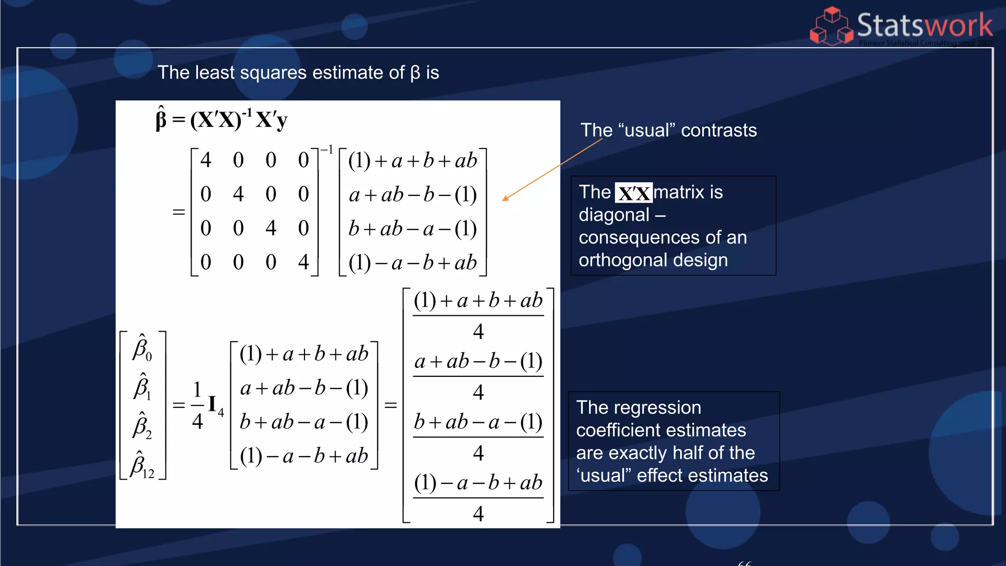
![Estimation of Factor Effects
1
2
1
2
1
2
(1)
2 2
[ (1)]
(1)
2 2
[ (1)]
(1)
2 2
[ (1) ]
A A
n
B B
n
n
A y y
ab a b
n n
ab a b
B y y
ab b a
n n
ab b a
ab a b
AB
n n
ab a b
See textbook, pg. 209-210 For
manual calculations
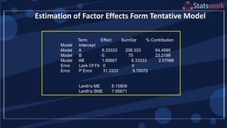
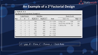
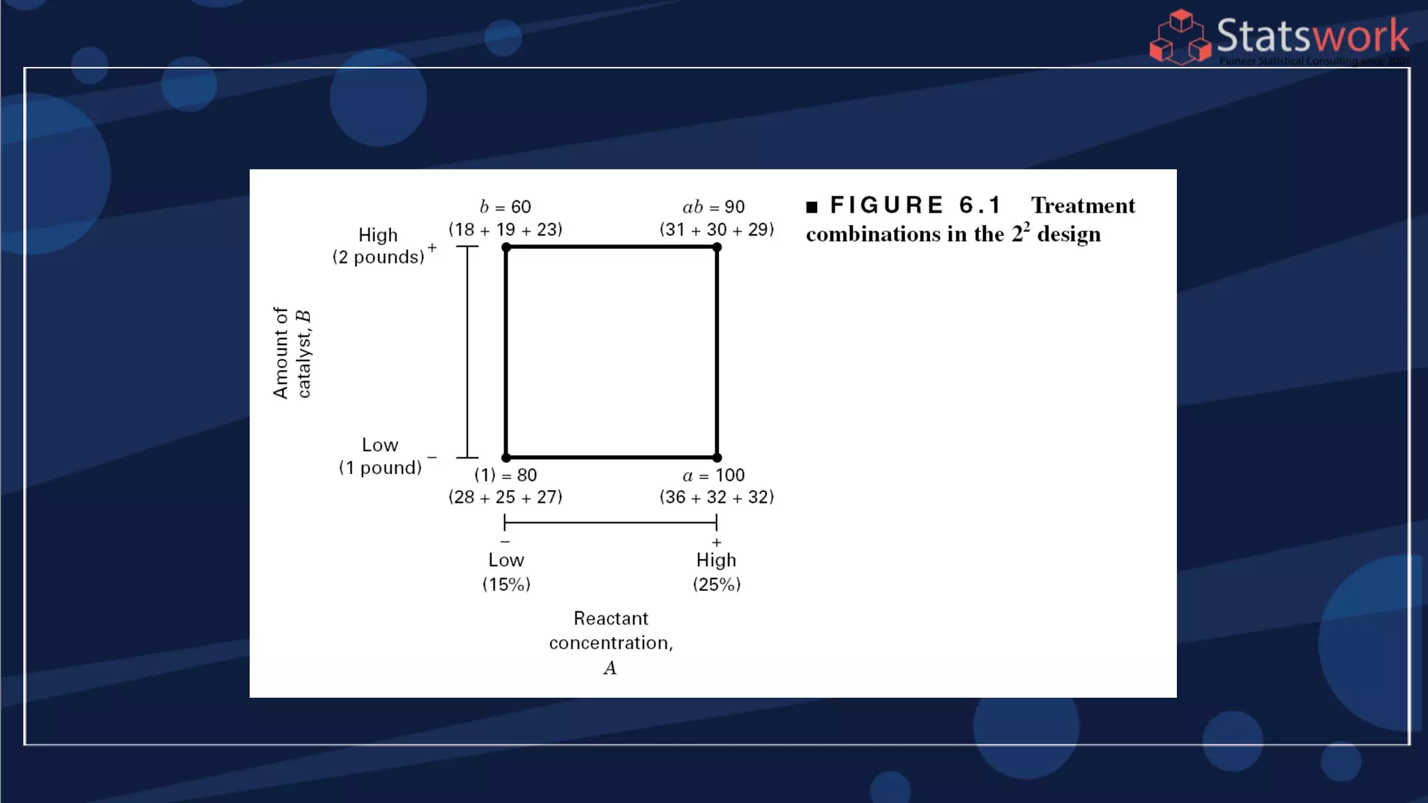
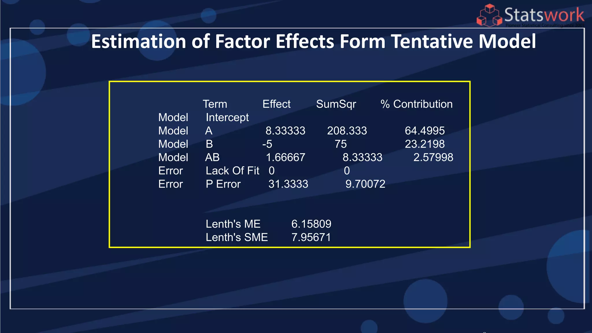
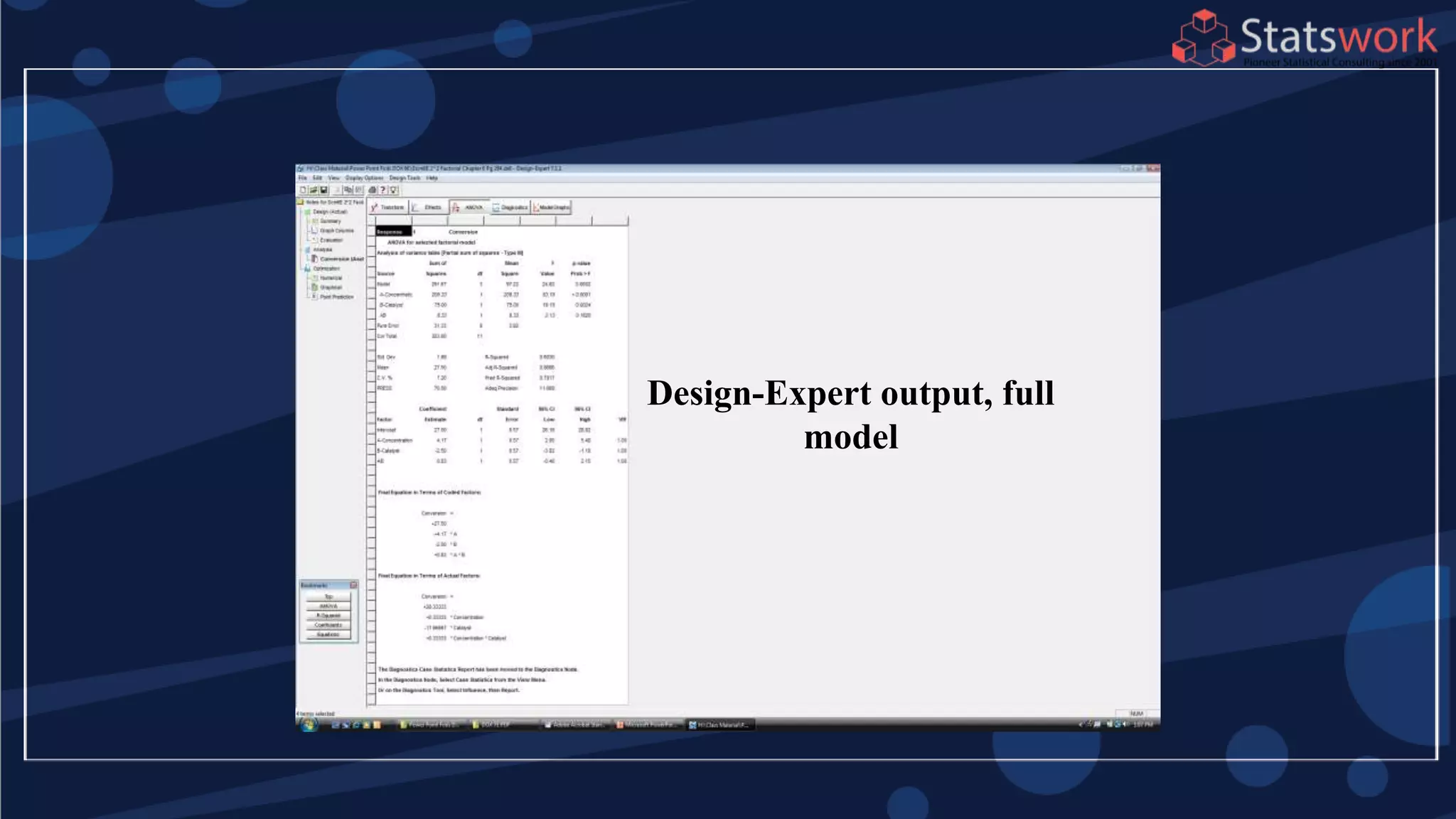
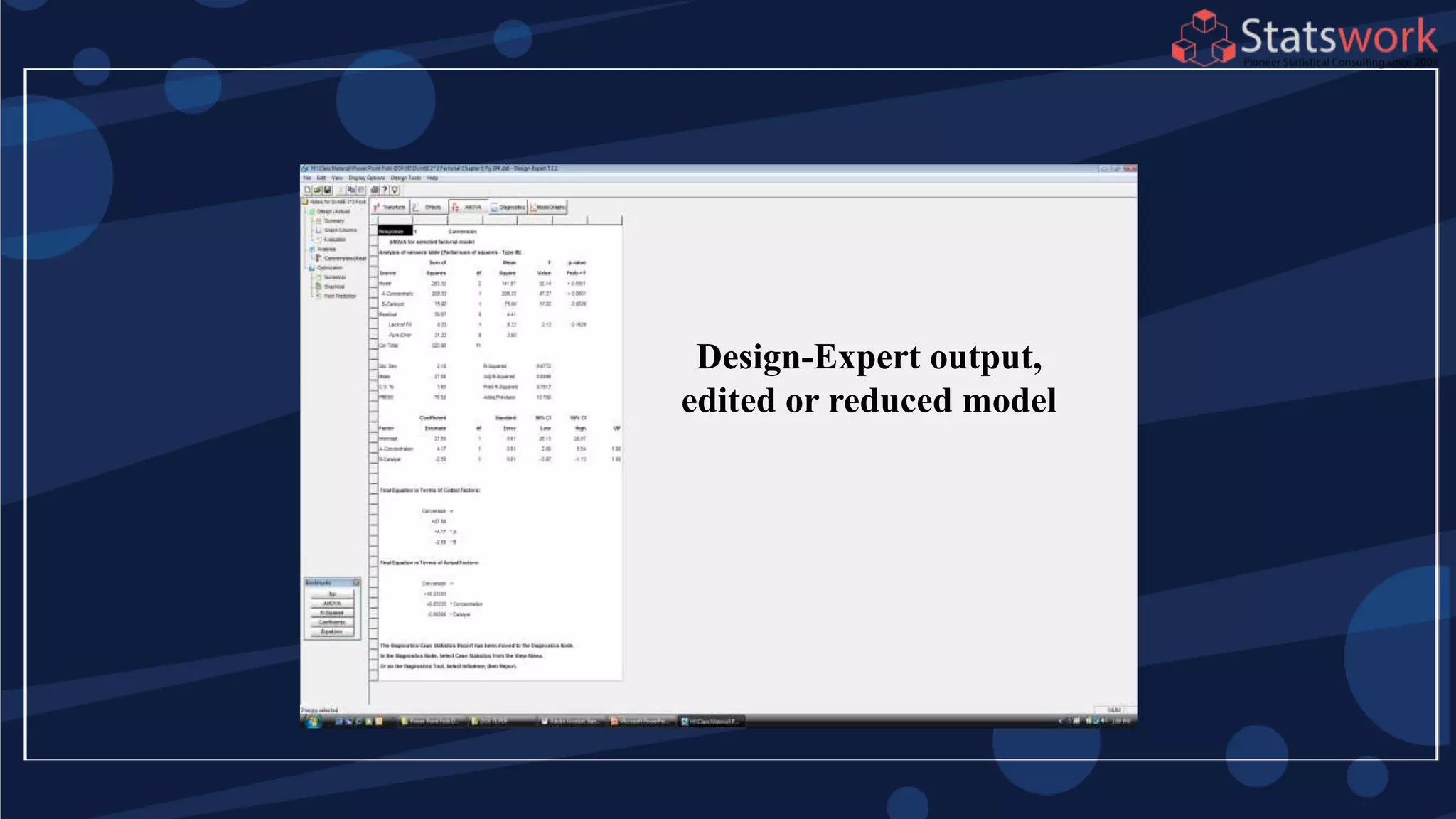
The effect estimates are: A
= 8.33, B = -5.00, AB = 1.67
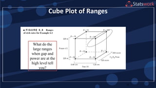
Practical interpretation?
Design-Expert analysis](https://image.slidesharecdn.com/designofengineeringexperimentspart5-190206074805/85/Design-of-Engineering-Experiments-Part-5-7-320.jpg)


![2
1 2
1 2 1 2
2
2 2 2 2
1 2 1 2 1 2
1 2
2
1 2
1 2
2
1 2
ˆ[ ( , )]
[1, , , ]
ˆ[ ( , )] (1 )
4
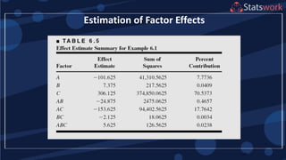
The maximum prediction variance occurs when 1, 1
ˆ[ ( , )]
The prediction variance when 0 is
ˆ[ ( , )]
V y x x
x x x x
V y x x x x x x
x x
V y x x
x x
V y x x
-1
x (X X) x
x
4
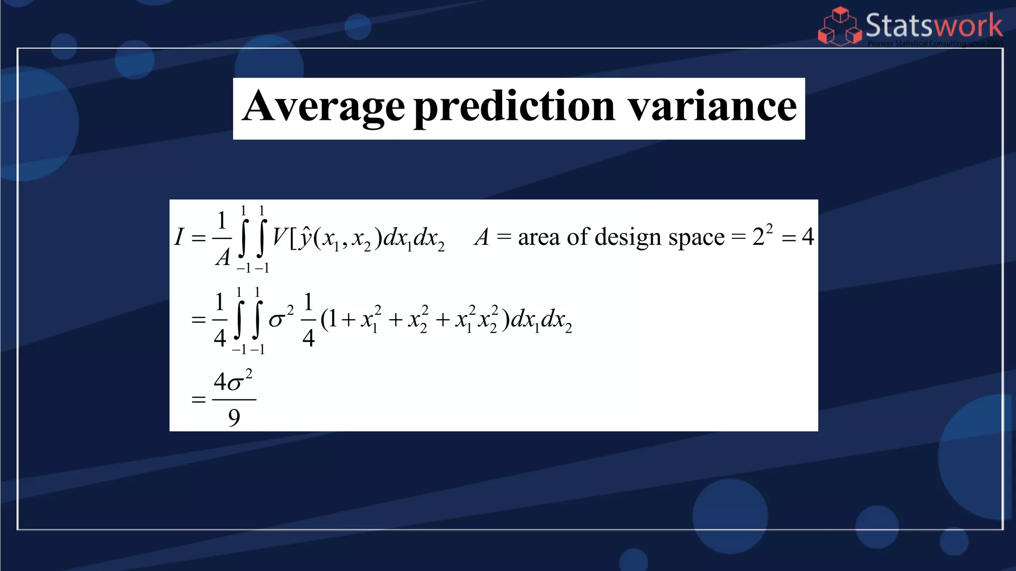
What about prediction variance over the design space?average](https://image.slidesharecdn.com/designofengineeringexperimentspart5-190206074805/85/Design-of-Engineering-Experiments-Part-5-68-320.jpg)


![Estimation of Factor Effects
1
2
1
2
1
2
(1)
2 2
[ (1)]
(1)
2 2
[ (1)]
(1)
2 2
[ (1) ]
A A
n
B B
n
n
A y y
ab a b
n n
ab a b
B y y
ab b a
n n
ab b a
ab a b
AB
n n
ab a b
See textbook, pg. 209-210 For
manual calculations
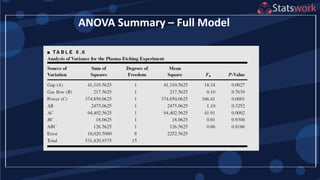
The effect estimates are: A
= 8.33, B = -5.00, AB = 1.67
Practical interpretation?
Design-Expert analysis](https://image.slidesharecdn.com/designofengineeringexperimentspart5-190206074805/75/Design-of-Engineering-Experiments-Part-5-7-2048.jpg)


![2
1 2
1 2 1 2
2
2 2 2 2
1 2 1 2 1 2
1 2
2
1 2
1 2
2
1 2
ˆ[ ( , )]
[1, , , ]
ˆ[ ( , )] (1 )
4
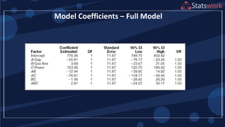
The maximum prediction variance occurs when 1, 1
ˆ[ ( , )]
The prediction variance when 0 is
ˆ[ ( , )]
V y x x
x x x x
V y x x x x x x
x x
V y x x
x x
V y x x
-1
x (X X) x
x
4
What about prediction variance over the design space?average](https://image.slidesharecdn.com/designofengineeringexperimentspart5-190206074805/75/Design-of-Engineering-Experiments-Part-5-68-2048.jpg)


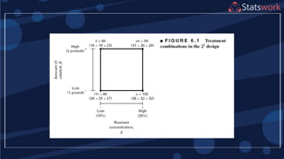
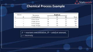
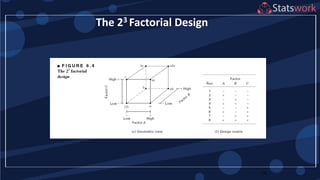
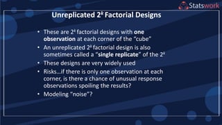
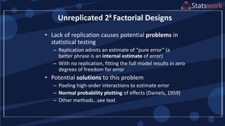
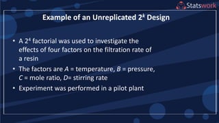
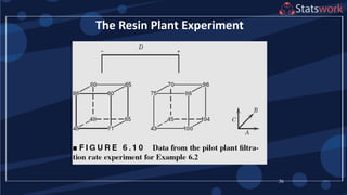
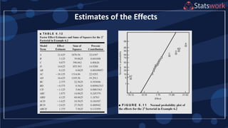
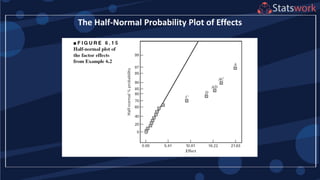
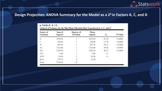
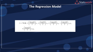
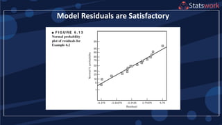
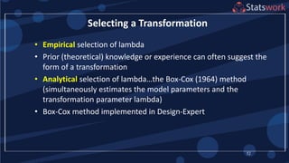
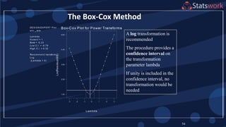
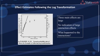
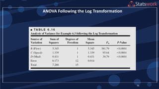
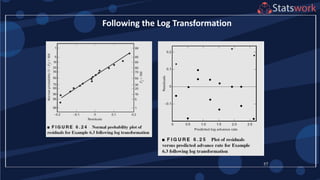
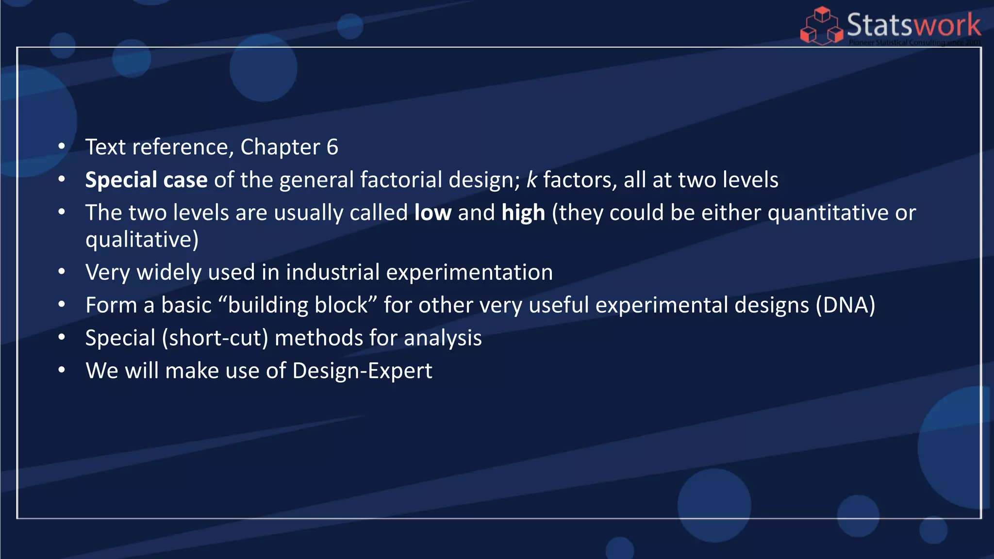
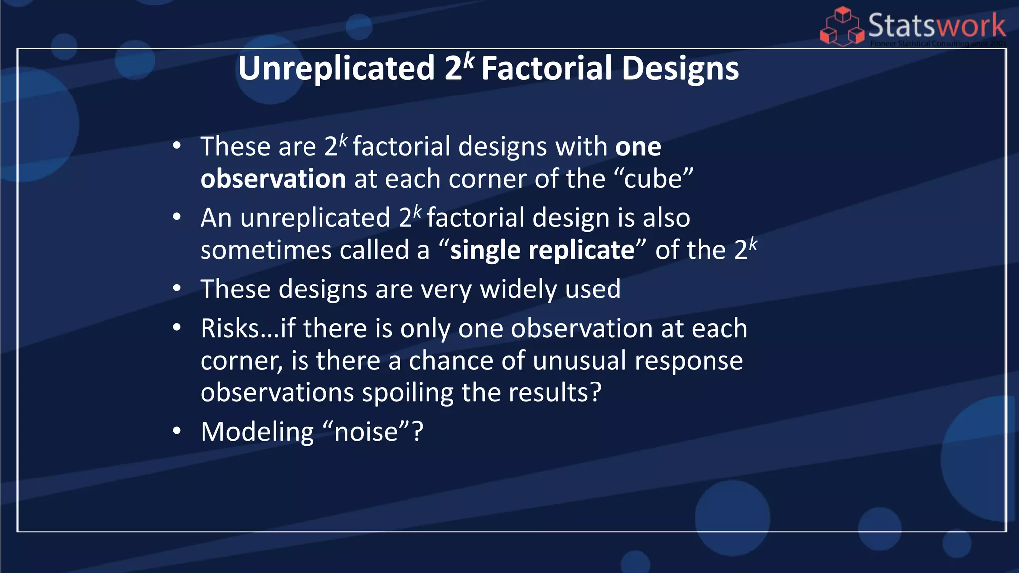
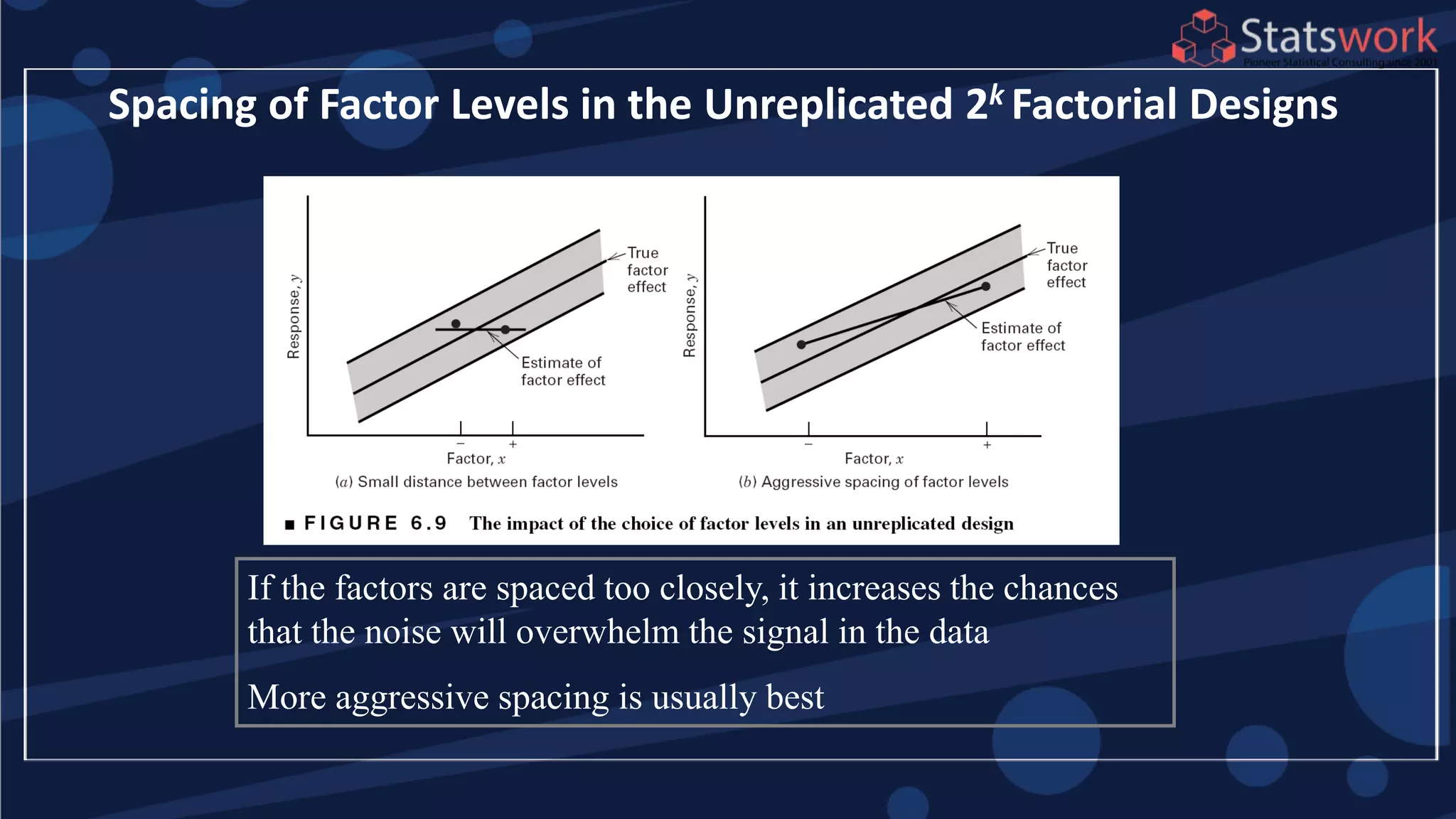
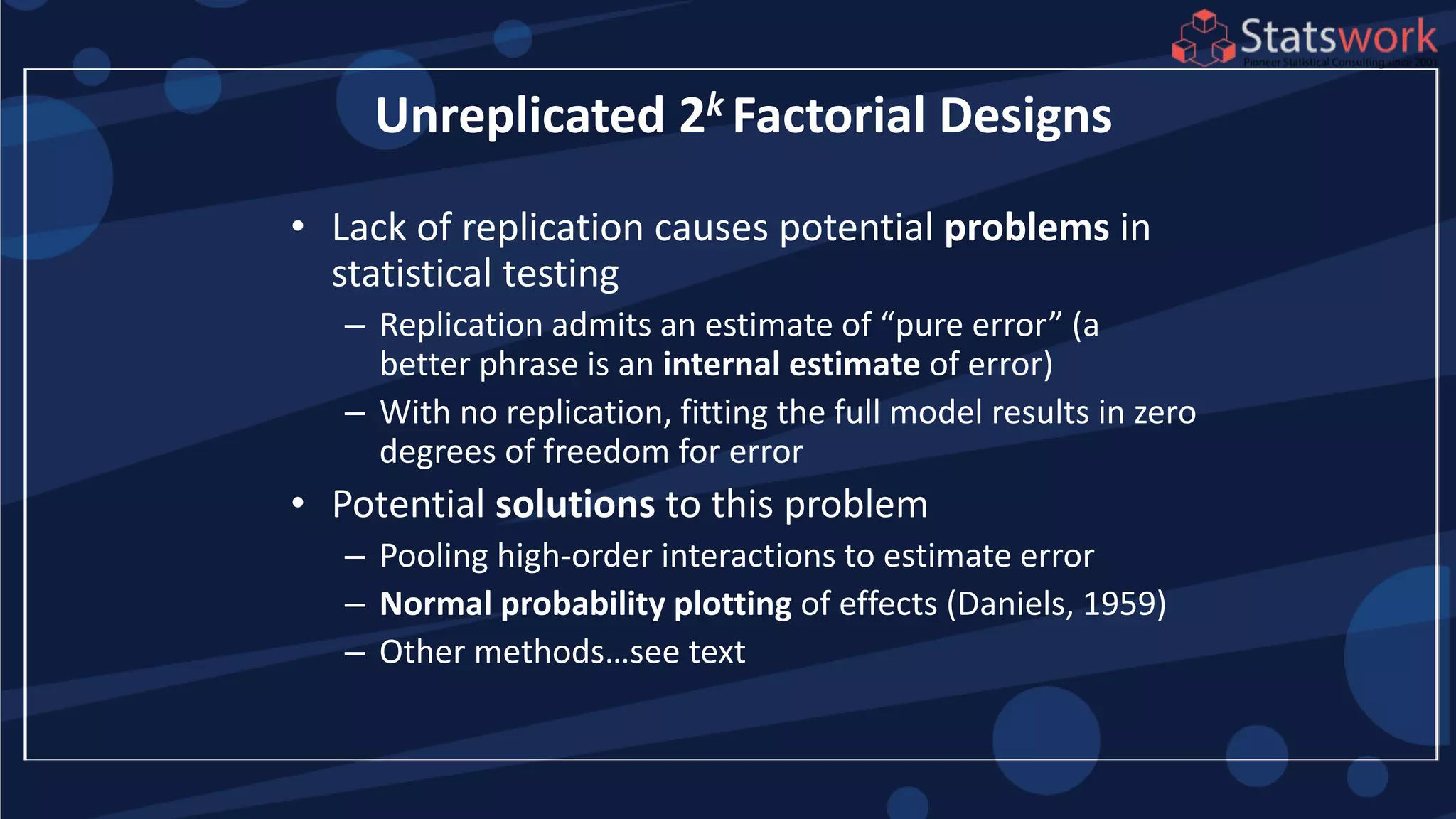
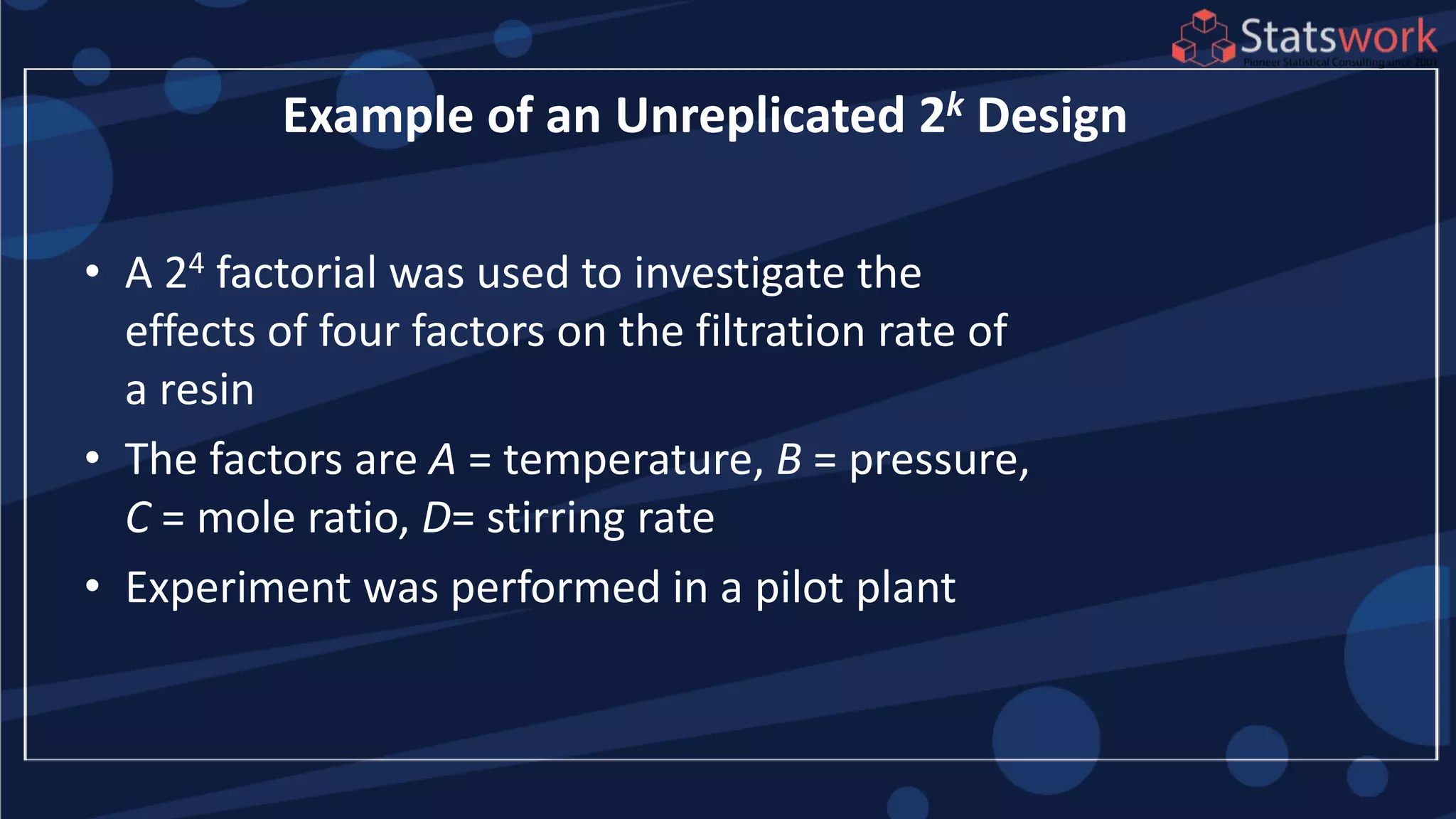
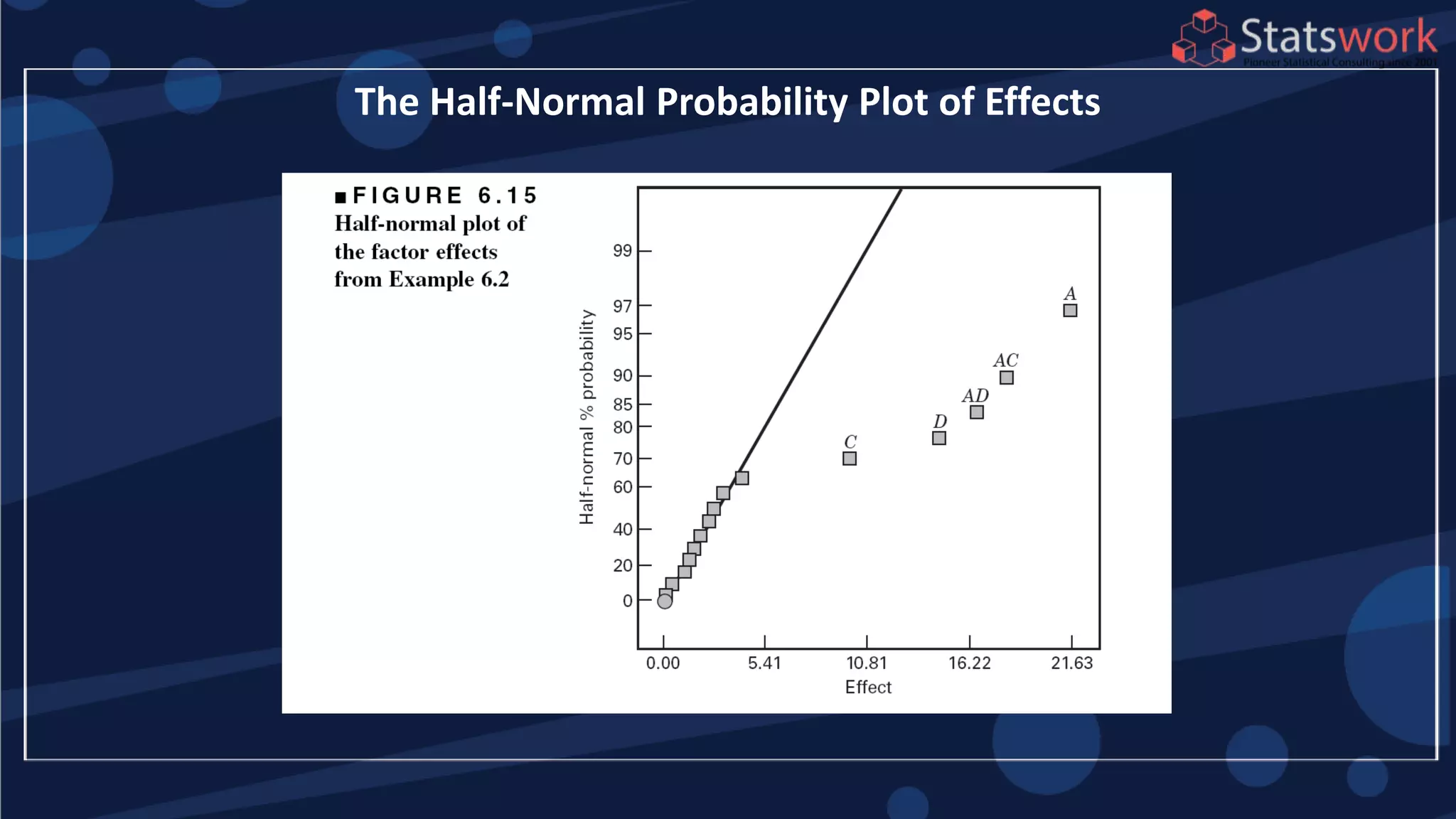
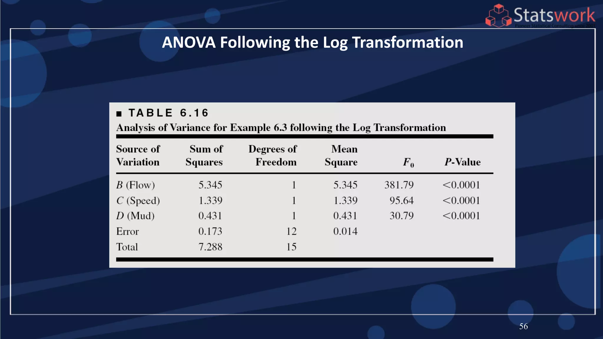
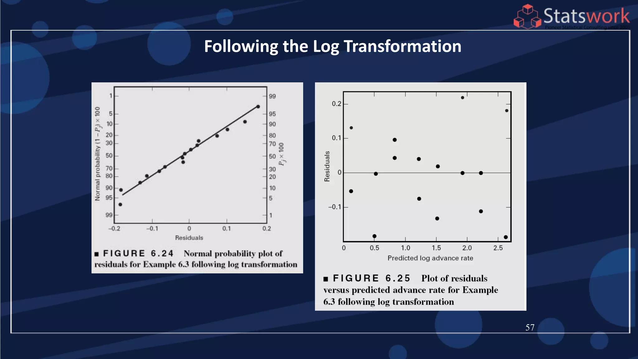
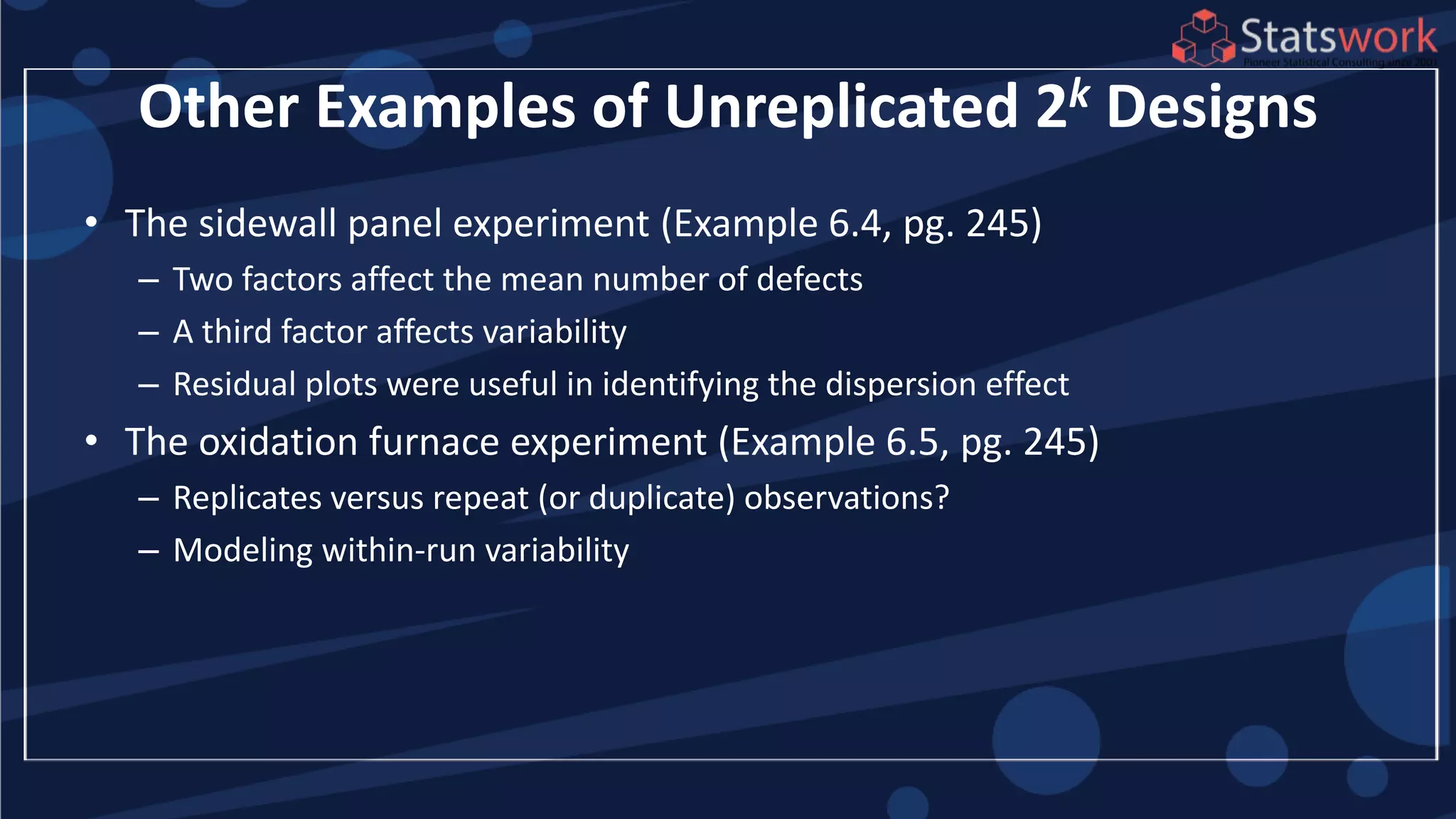
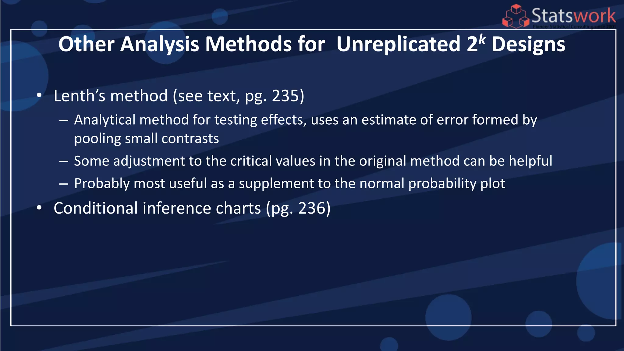
The document discusses the 2k factorial design, which is a special case of the general factorial design with k factors at two levels. It provides examples of using 2k factorial designs to investigate how multiple factors affect a response. For an unreplicated 2k design with no replication, there are challenges in statistical testing due to having zero degrees of freedom for error. Various methods are discussed for analyzing the effects in an unreplicated 2k design, such as normal probability plotting, Lenth's method, and conditional inference charts. Transformation of the response may also be needed to meet assumptions of the model such as equal variance.


