Downloaded 406 times


![Design
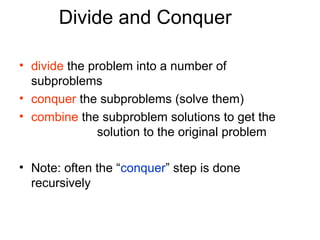
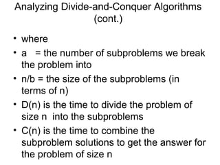
Follows the divide-and-conquer paradigm.
Divide: Partition (separate) the array A[p..r] into two
(possibly nonempty) subarrays A[p..q–1] and A[q+1..r].
Each element in A[p..q–1] ≤ A[q].
A[q] ≤ each element in A[q+1..r].
Index q is computed as part of the partitioning
procedure.
Conquer: Sort the two subarrays A[p..q–1] &
A[q+1..r] by recursive calls to quicksort.
Combine: Since the subarrays are sorted in place –
no work is needed to combine them.
How do the divide and combine steps of quicksort
compare with those of merge sort?](https://image.slidesharecdn.com/dinive-conqueralgorithm-130409103349-phpapp01/85/Dinive-conquer-algorithm-15-320.jpg)
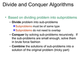
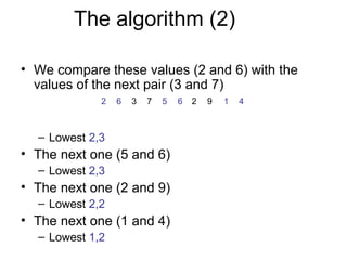
![Pseudocode
Quicksort(A, p, r)
Quicksort(A, p, r) Partition(A, p, r)
Partition(A, p, r)
if pp< rrthen
if < then x:= A[r],
x:= A[r],
qq:= Partition(A, p, r);
:= Partition(A, p, r); i i:=p – 1;
:=p – 1;
Quicksort(A, p, qq––1);
Quicksort(A, p, 1); for jj:= ppto rr––11do
for := to do
Quicksort(A, qq+ 1, r)
Quicksort(A, + 1, r) if A[j] ≤ xxthen
if A[j] ≤ then
fi
fi ii:= ii+ 1;
:= + 1;
A[i] ↔ A[j]
A[i] ↔ A[j]
A[p..r] fi
fi
od;
od;
5 A[i + 1] ↔ A[r];
A[i + 1] ↔ A[r];
return ii+ 11
return +
A[p..q – 1] A[q+1..r]
Partition 5
≤5 ≥5](https://image.slidesharecdn.com/dinive-conqueralgorithm-130409103349-phpapp01/85/Dinive-conquer-algorithm-16-320.jpg)
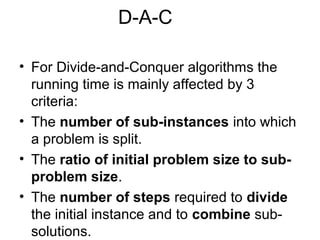
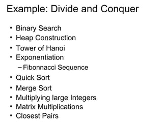
![Example
p r
initially: 2 5 8 3 9 4 1 7 10 6 note: pivot (x) = 6
i j
next iteration: 2 5 8 3 9 4 1 7 10 6
i j Partition(A, p, r)
Partition(A, p, r)
x, ii := A[r], pp––1;
x, := A[r], 1;
next iteration: 2 5 8 3 9 4 1 7 10 6 for jj:= ppto rr––11do
for := to do
i j if A[j] ≤ xxthen
if A[j] ≤ then
ii:= ii+ 1;
:= + 1;
next iteration: 2 5 8 3 9 4 1 7 10 6 A[i] ↔ A[j]
A[i] ↔ A[j]
i j fi
fi
od;
od;
next iteration: 2 5 3 8 9 4 1 7 10 6
A[i + 1] ↔ A[r];
A[i + 1] ↔ A[r];
i j
return ii+ 1
return + 1](https://image.slidesharecdn.com/dinive-conqueralgorithm-130409103349-phpapp01/85/Dinive-conquer-algorithm-17-320.jpg)
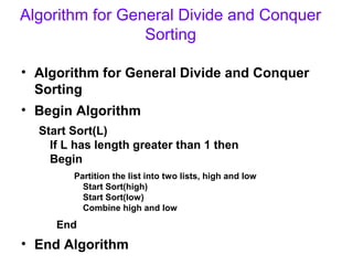
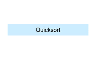
![Example (Continued)
next iteration: 2 5 3 8 9 4 1 7 10 6
i j
next iteration: 2 5 3 8 9 4 1 7 10 6
i j
next iteration: 2 5 3 4 9 8 1 7 10 6
Partition(A, p, r)
Partition(A, p, r)
i j
x, ii := A[r], pp––1;
x, := A[r], 1;
next iteration: 2 5 3 4 1 8 9 7 10 6 for jj:= ppto rr––11do
for := to do
i j if A[j] ≤ xxthen
if A[j] ≤ then
ii:= ii+ 1;
:= + 1;
next iteration: 2 5 3 4 1 8 9 7 10 6 A[i] ↔ A[j]
A[i] ↔ A[j]
i j fi
fi
od;
od;
next iteration: 2 5 3 4 1 8 9 7 10 6
A[i + 1] ↔ A[r];
A[i + 1] ↔ A[r];
i j
return ii+ 1
return + 1
after final swap: 2 5 3 4 1 6 9 7 10 8
i j](https://image.slidesharecdn.com/dinive-conqueralgorithm-130409103349-phpapp01/85/Dinive-conquer-algorithm-18-320.jpg)
![Partitioning
Select the last element A[r] in the subarray A[p..r] as
the pivot – the element around which to partition.
As the procedure executes, the array is partitioned
into four (possibly empty) regions.
1. A[p..i] — All entries in this region are ≤ pivot.
2. A[i+1..j – 1] — All entries in this region are > pivot.
3. A[r] = pivot.
4. A[j..r – 1] — Not known how they compare to pivot.
The above hold before each iteration of the for loop,
and constitute a loop invariant. (4 is not part of the LI.)](https://image.slidesharecdn.com/dinive-conqueralgorithm-130409103349-phpapp01/85/Dinive-conquer-algorithm-19-320.jpg)
![Correctness of Partition
Use loop invariant.
Initialization:
– Before first iteration
• A[p..i] and A[i+1..j – 1] are empty – Conds. 1 and 2 are
satisfied (trivially). Partition(A, p, r)
Partition(A, p, r)
x, i := A[r], p – 1;
• r is the index of the pivot – Cond. 3 is forij := p to r p – 1;
x, := A[r],
satisfied. – 1 do
for j := p to r – 1 do
Maintenance: if A[j] ≤ xxthen
if A[j] ≤ then
ii:= ii+ 1;
:= + 1;
– Case 1: A[j] > x A[i] ↔ A[j]
A[i] ↔ A[j]
• Increment j only. fi
fi
od;
od;
• LI is maintained. A[i + 1] ↔ A[r];
A[i + 1] ↔ A[r];
return ii+ 11
return +](https://image.slidesharecdn.com/dinive-conqueralgorithm-130409103349-phpapp01/85/Dinive-conquer-algorithm-20-320.jpg)
![Correctness of Partition
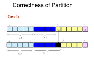
• Case 2: A[j] ≤ x
– Increment i – A[r] is unaltered.
– Swap A[i] and A[j] • Condition 3 is maintained.
• Condition 1 is maintained.
– Increment j
• Condition 2 is maintained.
p i j r
≤x x
≤x >x
p i j r
x
≤x >x](https://image.slidesharecdn.com/dinive-conqueralgorithm-130409103349-phpapp01/85/Dinive-conquer-algorithm-22-320.jpg)
![Correctness of Partition
Termination:
– When the loop terminates, j = r, so all elements in A are
partitioned into one of the three cases:
• A[p..i] ≤ pivot
• A[i+1..j – 1] > pivot
• A[r] = pivot
The last two lines swap A[i+1] and A[r].
– Pivot moves from the end of the array to between the
two subarrays.
– Thus, procedure partition correctly performs the divide
step.](https://image.slidesharecdn.com/dinive-conqueralgorithm-130409103349-phpapp01/85/Dinive-conquer-algorithm-23-320.jpg)
![Complexity of Partition
• PartitionTime(n) is given by the number of
iterations in the for loop.
∀ Θ(n) : n = r – p + 1. Partition(A, p, r)
Partition(A, p, r)
x, ii := A[r], pp––1;
x, := A[r], 1;
for jj:= ppto rr––11do
for := to do
if A[j] ≤ xxthen
if A[j] ≤ then
ii:= ii+ 1;
:= + 1;
A[i] ↔ A[j]
A[i] ↔ A[j]
fi
fi
od;
od;
A[i + 1] ↔ A[r];
A[i + 1] ↔ A[r];
return ii+ 1
return + 1](https://image.slidesharecdn.com/dinive-conqueralgorithm-130409103349-phpapp01/85/Dinive-conquer-algorithm-24-320.jpg)
![Algorithm Performance
• Running time of quicksort depends on whether the
partitioning is balanced or not.
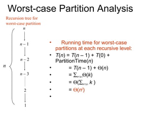
• Worst-Case Partitioning (Unbalanced Partitions):
– Occurs when every call to partition results in the most
unbalanced partition.
– Partition is most unbalanced when
• Subproblem 1 is of size n – 1, and subproblem 2 is of size 0
or vice versa.
• pivot ≥ every element in A[p..r – 1] or pivot < every element in
A[p..r – 1].
– Every call to partition is most unbalanced when
• Array A[1..n] is sorted or reverse sorted!](https://image.slidesharecdn.com/dinive-conqueralgorithm-130409103349-phpapp01/85/Dinive-conquer-algorithm-25-320.jpg)


![Merge-Sort (A, p, r)
• INPUT: a sequence of n numbers stored in
array A
MergeSort (A, p, r) // sort A[p..r] by divide & conquer
• if p < r
1 OUTPUT: an ordered sequence of n
2 numbers (p+r)/2
then q ←
3 MergeSort (A, p, q)
4 MergeSort (A, q+1, r)
5 Merge (A, p, q, r) // merges A[p..q] with A[q+1..r]
Initial Call: MergeSort(A, 1, n)](https://image.slidesharecdn.com/dinive-conqueralgorithm-130409103349-phpapp01/85/Dinive-conquer-algorithm-34-320.jpg)
![Procedure Merge
• Merge(A, p, q, r)
• 1 n1 ← q – p + 1 Input: Array containing
• 2 n2 ← r – q sorted subarrays A[p..q]
for i ← 1 to n1 and A[q+1..r].
do L[i] ← A[p + i – 1] Output: Merged sorted
for j ← 1 to n2
subarray in A[p..r].
do R[j] ← A[q + j]
L[n1+1] ← ∞
R[n2+1] ← ∞
i←1
j←1 Sentinels, to avoid having to
for k ←p to r check if either subarray is
do if L[i] ≤ R[j] fully copied at each step.
then A[k] ← L[i]
i←i+1
else A[k] ← R[j]
j←j+1](https://image.slidesharecdn.com/dinive-conqueralgorithm-130409103349-phpapp01/85/Dinive-conquer-algorithm-35-320.jpg)
![Correctness of Merge
• Merge(A, p, q, r)
Loop Invariant for the for loop
• 1 n1 ← q – p + 1 At the start of each iteration of the
• 2 n2 ← r – q for loop:
for i ← 1 to n1 Subarray A[p..k – 1]
do L[i] ← A[p + i – 1] contains the k – p smallest elements
for j ← 1 to n2 of L and R in sorted order.
L[i] and R[j] are the smallest elements of
do R[j] ← A[q + j] L and R that have not been copied back into
L[n1+1] ← ∞ A.
R[n2+1] ← ∞
i←1 Initialization:
j←1 Before the first iteration:
•A[p..k – 1] is empty.
for k ←p to r
•i = j = 1.
do if L[i] ≤ R[j]
•L[1] and R[1] are the smallest
then A[k] ← L[i] elements of L and R not copied to A.
i←i+1
else A[k] ← R[j]](https://image.slidesharecdn.com/dinive-conqueralgorithm-130409103349-phpapp01/85/Dinive-conquer-algorithm-37-320.jpg)
![Correctness of Merge
• Merge(A, p, q, r) Maintenance:
• 1 n1 ← q – p + 1 Case 1: L[i] ≤ R[j]
•By LI, A contains p – k smallest elements
• 2 n2 ← r – q
of L and R in sorted order.
for i ← 1 to n1 •By LI, L[i] and R[j] are the smallest elements
do L[i] ← A[p + i – 1] of L and R not yet copied into A.
for j ← 1 to n2 •Line 13 results in A containing p – k + 1
smallest elements (again in sorted order).
do R[j] ← A[q + j] Incrementing i and k reestablishes the LI for
L[n1+1] ← ∞ the next iteration.
R[n2+1] ← ∞ Similarly for L[i] > R[j].
i←1 Termination:
j←1 •On termination, k = r + 1.
for k ←p to r •By LI, A contains r – p + 1 smallest
do if L[i] ≤ R[j] elements of L and R in sorted order.
then A[k] ← L[i] •L and R together contain r – p + 3 elements.
All but the two sentinels have been copied
i←i+1
back into A.
else A[k] ← R[j]
](https://image.slidesharecdn.com/dinive-conqueralgorithm-130409103349-phpapp01/85/Dinive-conquer-algorithm-38-320.jpg)


![Design
Follows the divide-and-conquer paradigm.
Divide: Partition (separate) the array A[p..r] into two
(possibly nonempty) subarrays A[p..q–1] and A[q+1..r].
Each element in A[p..q–1] ≤ A[q].
A[q] ≤ each element in A[q+1..r].
Index q is computed as part of the partitioning
procedure.
Conquer: Sort the two subarrays A[p..q–1] &
A[q+1..r] by recursive calls to quicksort.
Combine: Since the subarrays are sorted in place –
no work is needed to combine them.
How do the divide and combine steps of quicksort
compare with those of merge sort?](https://image.slidesharecdn.com/dinive-conqueralgorithm-130409103349-phpapp01/75/Dinive-conquer-algorithm-15-2048.jpg)
![Pseudocode
Quicksort(A, p, r)
Quicksort(A, p, r) Partition(A, p, r)
Partition(A, p, r)
if pp< rrthen
if < then x:= A[r],
x:= A[r],
qq:= Partition(A, p, r);
:= Partition(A, p, r); i i:=p – 1;
:=p – 1;
Quicksort(A, p, qq––1);
Quicksort(A, p, 1); for jj:= ppto rr––11do
for := to do
Quicksort(A, qq+ 1, r)
Quicksort(A, + 1, r) if A[j] ≤ xxthen
if A[j] ≤ then
fi
fi ii:= ii+ 1;
:= + 1;
A[i] ↔ A[j]
A[i] ↔ A[j]
A[p..r] fi
fi
od;
od;
5 A[i + 1] ↔ A[r];
A[i + 1] ↔ A[r];
return ii+ 11
return +
A[p..q – 1] A[q+1..r]
Partition 5
≤5 ≥5](https://image.slidesharecdn.com/dinive-conqueralgorithm-130409103349-phpapp01/75/Dinive-conquer-algorithm-16-2048.jpg)
![Example
p r
initially: 2 5 8 3 9 4 1 7 10 6 note: pivot (x) = 6
i j
next iteration: 2 5 8 3 9 4 1 7 10 6
i j Partition(A, p, r)
Partition(A, p, r)
x, ii := A[r], pp––1;
x, := A[r], 1;
next iteration: 2 5 8 3 9 4 1 7 10 6 for jj:= ppto rr––11do
for := to do
i j if A[j] ≤ xxthen
if A[j] ≤ then
ii:= ii+ 1;
:= + 1;
next iteration: 2 5 8 3 9 4 1 7 10 6 A[i] ↔ A[j]
A[i] ↔ A[j]
i j fi
fi
od;
od;
next iteration: 2 5 3 8 9 4 1 7 10 6
A[i + 1] ↔ A[r];
A[i + 1] ↔ A[r];
i j
return ii+ 1
return + 1](https://image.slidesharecdn.com/dinive-conqueralgorithm-130409103349-phpapp01/75/Dinive-conquer-algorithm-17-2048.jpg)
![Example (Continued)
next iteration: 2 5 3 8 9 4 1 7 10 6
i j
next iteration: 2 5 3 8 9 4 1 7 10 6
i j
next iteration: 2 5 3 4 9 8 1 7 10 6
Partition(A, p, r)
Partition(A, p, r)
i j
x, ii := A[r], pp––1;
x, := A[r], 1;
next iteration: 2 5 3 4 1 8 9 7 10 6 for jj:= ppto rr––11do
for := to do
i j if A[j] ≤ xxthen
if A[j] ≤ then
ii:= ii+ 1;
:= + 1;
next iteration: 2 5 3 4 1 8 9 7 10 6 A[i] ↔ A[j]
A[i] ↔ A[j]
i j fi
fi
od;
od;
next iteration: 2 5 3 4 1 8 9 7 10 6
A[i + 1] ↔ A[r];
A[i + 1] ↔ A[r];
i j
return ii+ 1
return + 1
after final swap: 2 5 3 4 1 6 9 7 10 8
i j](https://image.slidesharecdn.com/dinive-conqueralgorithm-130409103349-phpapp01/75/Dinive-conquer-algorithm-18-2048.jpg)
![Partitioning
Select the last element A[r] in the subarray A[p..r] as
the pivot – the element around which to partition.
As the procedure executes, the array is partitioned
into four (possibly empty) regions.
1. A[p..i] — All entries in this region are ≤ pivot.
2. A[i+1..j – 1] — All entries in this region are > pivot.
3. A[r] = pivot.
4. A[j..r – 1] — Not known how they compare to pivot.
The above hold before each iteration of the for loop,
and constitute a loop invariant. (4 is not part of the LI.)](https://image.slidesharecdn.com/dinive-conqueralgorithm-130409103349-phpapp01/75/Dinive-conquer-algorithm-19-2048.jpg)
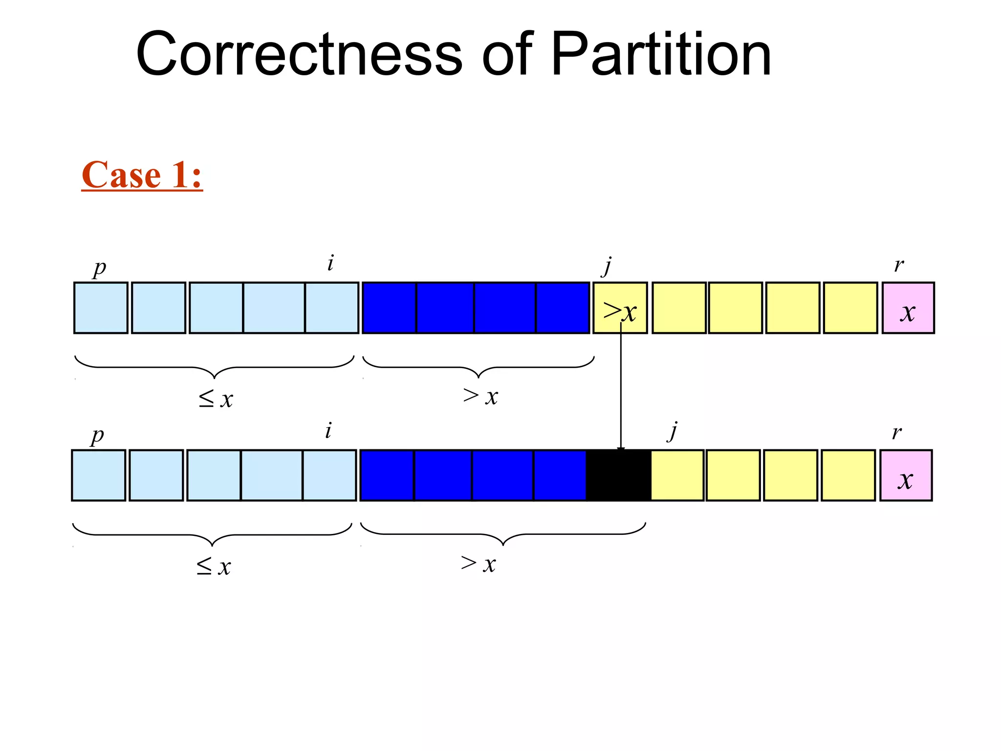
![Correctness of Partition
Use loop invariant.
Initialization:
– Before first iteration
• A[p..i] and A[i+1..j – 1] are empty – Conds. 1 and 2 are
satisfied (trivially). Partition(A, p, r)
Partition(A, p, r)
x, i := A[r], p – 1;
• r is the index of the pivot – Cond. 3 is forij := p to r p – 1;
x, := A[r],
satisfied. – 1 do
for j := p to r – 1 do
Maintenance: if A[j] ≤ xxthen
if A[j] ≤ then
ii:= ii+ 1;
:= + 1;
– Case 1: A[j] > x A[i] ↔ A[j]
A[i] ↔ A[j]
• Increment j only. fi
fi
od;
od;
• LI is maintained. A[i + 1] ↔ A[r];
A[i + 1] ↔ A[r];
return ii+ 11
return +](https://image.slidesharecdn.com/dinive-conqueralgorithm-130409103349-phpapp01/75/Dinive-conquer-algorithm-20-2048.jpg)
![Correctness of Partition
• Case 2: A[j] ≤ x
– Increment i – A[r] is unaltered.
– Swap A[i] and A[j] • Condition 3 is maintained.
• Condition 1 is maintained.
– Increment j
• Condition 2 is maintained.
p i j r
≤x x
≤x >x
p i j r
x
≤x >x](https://image.slidesharecdn.com/dinive-conqueralgorithm-130409103349-phpapp01/75/Dinive-conquer-algorithm-22-2048.jpg)
![Correctness of Partition
Termination:
– When the loop terminates, j = r, so all elements in A are
partitioned into one of the three cases:
• A[p..i] ≤ pivot
• A[i+1..j – 1] > pivot
• A[r] = pivot
The last two lines swap A[i+1] and A[r].
– Pivot moves from the end of the array to between the
two subarrays.
– Thus, procedure partition correctly performs the divide
step.](https://image.slidesharecdn.com/dinive-conqueralgorithm-130409103349-phpapp01/75/Dinive-conquer-algorithm-23-2048.jpg)
![Complexity of Partition
• PartitionTime(n) is given by the number of
iterations in the for loop.
∀ Θ(n) : n = r – p + 1. Partition(A, p, r)
Partition(A, p, r)
x, ii := A[r], pp––1;
x, := A[r], 1;
for jj:= ppto rr––11do
for := to do
if A[j] ≤ xxthen
if A[j] ≤ then
ii:= ii+ 1;
:= + 1;
A[i] ↔ A[j]
A[i] ↔ A[j]
fi
fi
od;
od;
A[i + 1] ↔ A[r];
A[i + 1] ↔ A[r];
return ii+ 1
return + 1](https://image.slidesharecdn.com/dinive-conqueralgorithm-130409103349-phpapp01/75/Dinive-conquer-algorithm-24-2048.jpg)
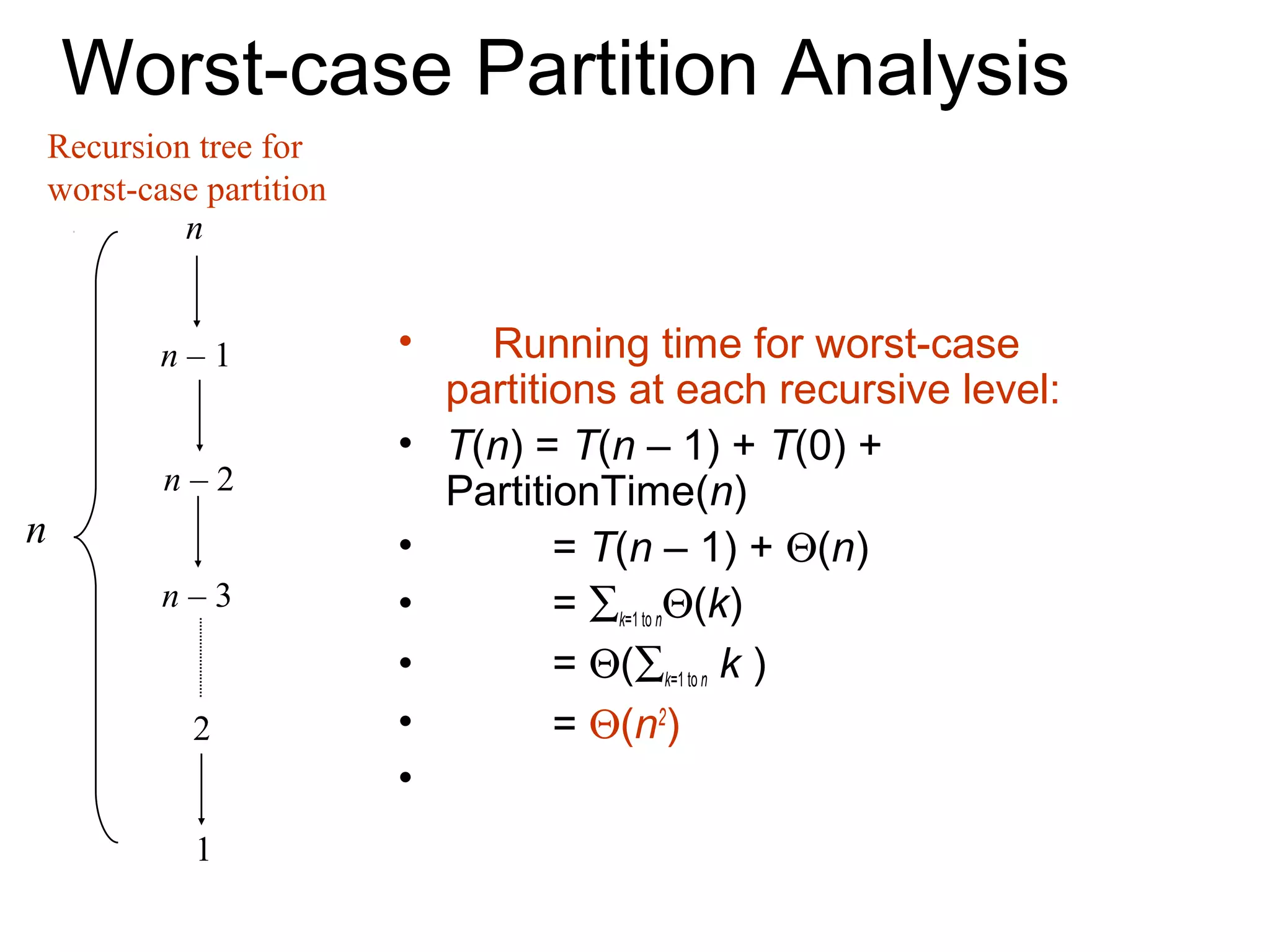
![Algorithm Performance
• Running time of quicksort depends on whether the
partitioning is balanced or not.
• Worst-Case Partitioning (Unbalanced Partitions):
– Occurs when every call to partition results in the most
unbalanced partition.
– Partition is most unbalanced when
• Subproblem 1 is of size n – 1, and subproblem 2 is of size 0
or vice versa.
• pivot ≥ every element in A[p..r – 1] or pivot < every element in
A[p..r – 1].
– Every call to partition is most unbalanced when
• Array A[1..n] is sorted or reverse sorted!](https://image.slidesharecdn.com/dinive-conqueralgorithm-130409103349-phpapp01/75/Dinive-conquer-algorithm-25-2048.jpg)
![Merge-Sort (A, p, r)
• INPUT: a sequence of n numbers stored in
array A
MergeSort (A, p, r) // sort A[p..r] by divide & conquer
• if p < r
1 OUTPUT: an ordered sequence of n
2 numbers (p+r)/2
then q ←
3 MergeSort (A, p, q)
4 MergeSort (A, q+1, r)
5 Merge (A, p, q, r) // merges A[p..q] with A[q+1..r]
Initial Call: MergeSort(A, 1, n)](https://image.slidesharecdn.com/dinive-conqueralgorithm-130409103349-phpapp01/75/Dinive-conquer-algorithm-34-2048.jpg)
![Procedure Merge
• Merge(A, p, q, r)
• 1 n1 ← q – p + 1 Input: Array containing
• 2 n2 ← r – q sorted subarrays A[p..q]
for i ← 1 to n1 and A[q+1..r].
do L[i] ← A[p + i – 1] Output: Merged sorted
for j ← 1 to n2
subarray in A[p..r].
do R[j] ← A[q + j]
L[n1+1] ← ∞
R[n2+1] ← ∞
i←1
j←1 Sentinels, to avoid having to
for k ←p to r check if either subarray is
do if L[i] ≤ R[j] fully copied at each step.
then A[k] ← L[i]
i←i+1
else A[k] ← R[j]
j←j+1](https://image.slidesharecdn.com/dinive-conqueralgorithm-130409103349-phpapp01/75/Dinive-conquer-algorithm-35-2048.jpg)
![Correctness of Merge
• Merge(A, p, q, r)
Loop Invariant for the for loop
• 1 n1 ← q – p + 1 At the start of each iteration of the
• 2 n2 ← r – q for loop:
for i ← 1 to n1 Subarray A[p..k – 1]
do L[i] ← A[p + i – 1] contains the k – p smallest elements
for j ← 1 to n2 of L and R in sorted order.
L[i] and R[j] are the smallest elements of
do R[j] ← A[q + j] L and R that have not been copied back into
L[n1+1] ← ∞ A.
R[n2+1] ← ∞
i←1 Initialization:
j←1 Before the first iteration:
•A[p..k – 1] is empty.
for k ←p to r
•i = j = 1.
do if L[i] ≤ R[j]
•L[1] and R[1] are the smallest
then A[k] ← L[i] elements of L and R not copied to A.
i←i+1
else A[k] ← R[j]](https://image.slidesharecdn.com/dinive-conqueralgorithm-130409103349-phpapp01/75/Dinive-conquer-algorithm-37-2048.jpg)
![Correctness of Merge
• Merge(A, p, q, r) Maintenance:
• 1 n1 ← q – p + 1 Case 1: L[i] ≤ R[j]
•By LI, A contains p – k smallest elements
• 2 n2 ← r – q
of L and R in sorted order.
for i ← 1 to n1 •By LI, L[i] and R[j] are the smallest elements
do L[i] ← A[p + i – 1] of L and R not yet copied into A.
for j ← 1 to n2 •Line 13 results in A containing p – k + 1
smallest elements (again in sorted order).
do R[j] ← A[q + j] Incrementing i and k reestablishes the LI for
L[n1+1] ← ∞ the next iteration.
R[n2+1] ← ∞ Similarly for L[i] > R[j].
i←1 Termination:
j←1 •On termination, k = r + 1.
for k ←p to r •By LI, A contains r – p + 1 smallest
do if L[i] ≤ R[j] elements of L and R in sorted order.
then A[k] ← L[i] •L and R together contain r – p + 3 elements.
All but the two sentinels have been copied
i←i+1
back into A.
else A[k] ← R[j]
](https://image.slidesharecdn.com/dinive-conqueralgorithm-130409103349-phpapp01/75/Dinive-conquer-algorithm-38-2048.jpg)

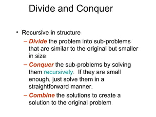
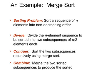
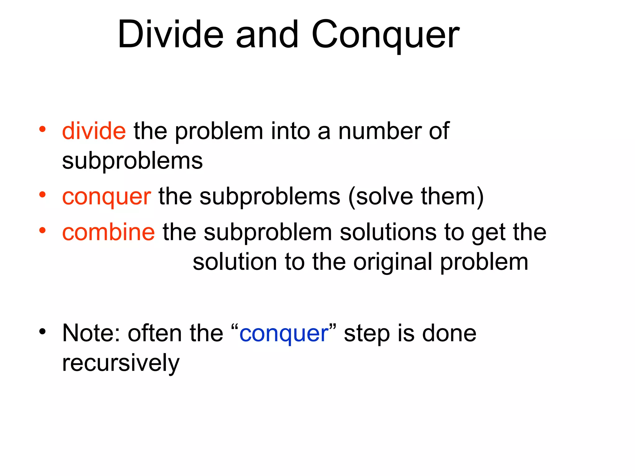
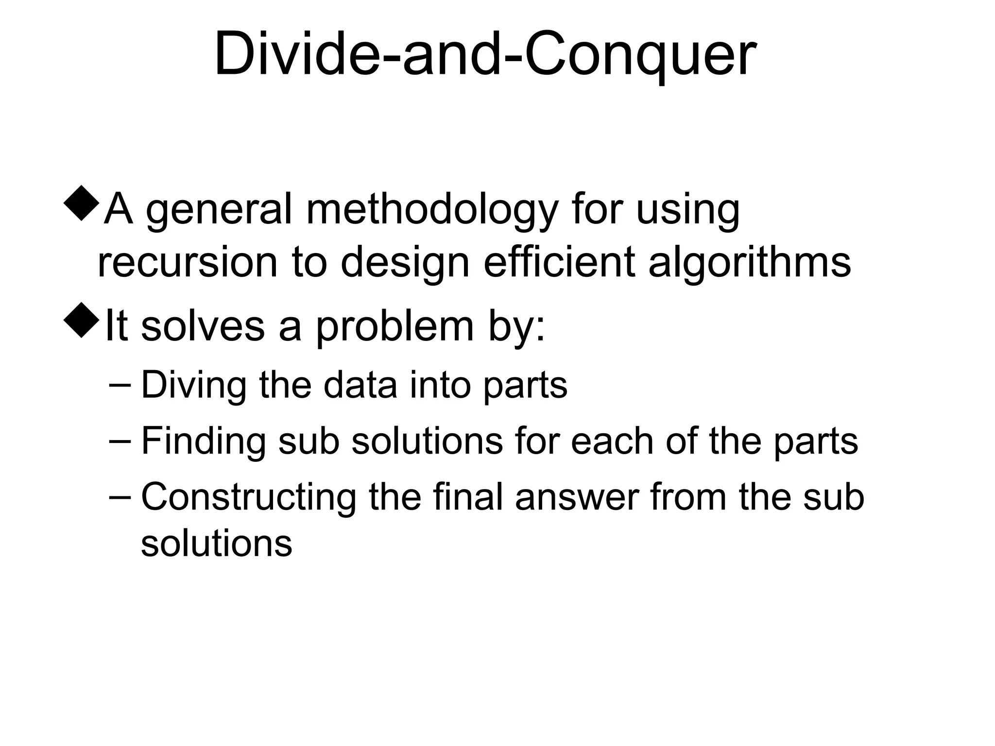
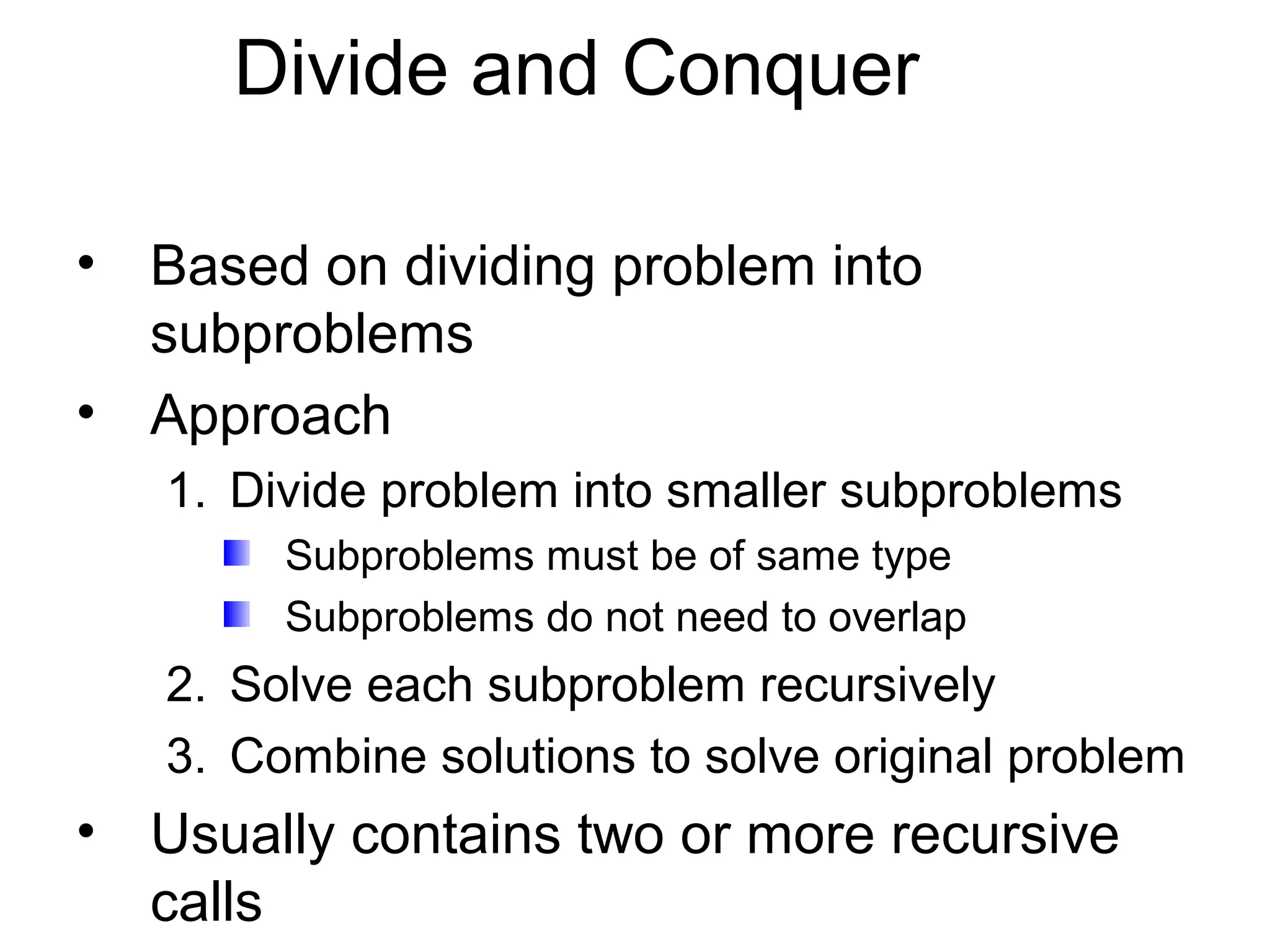
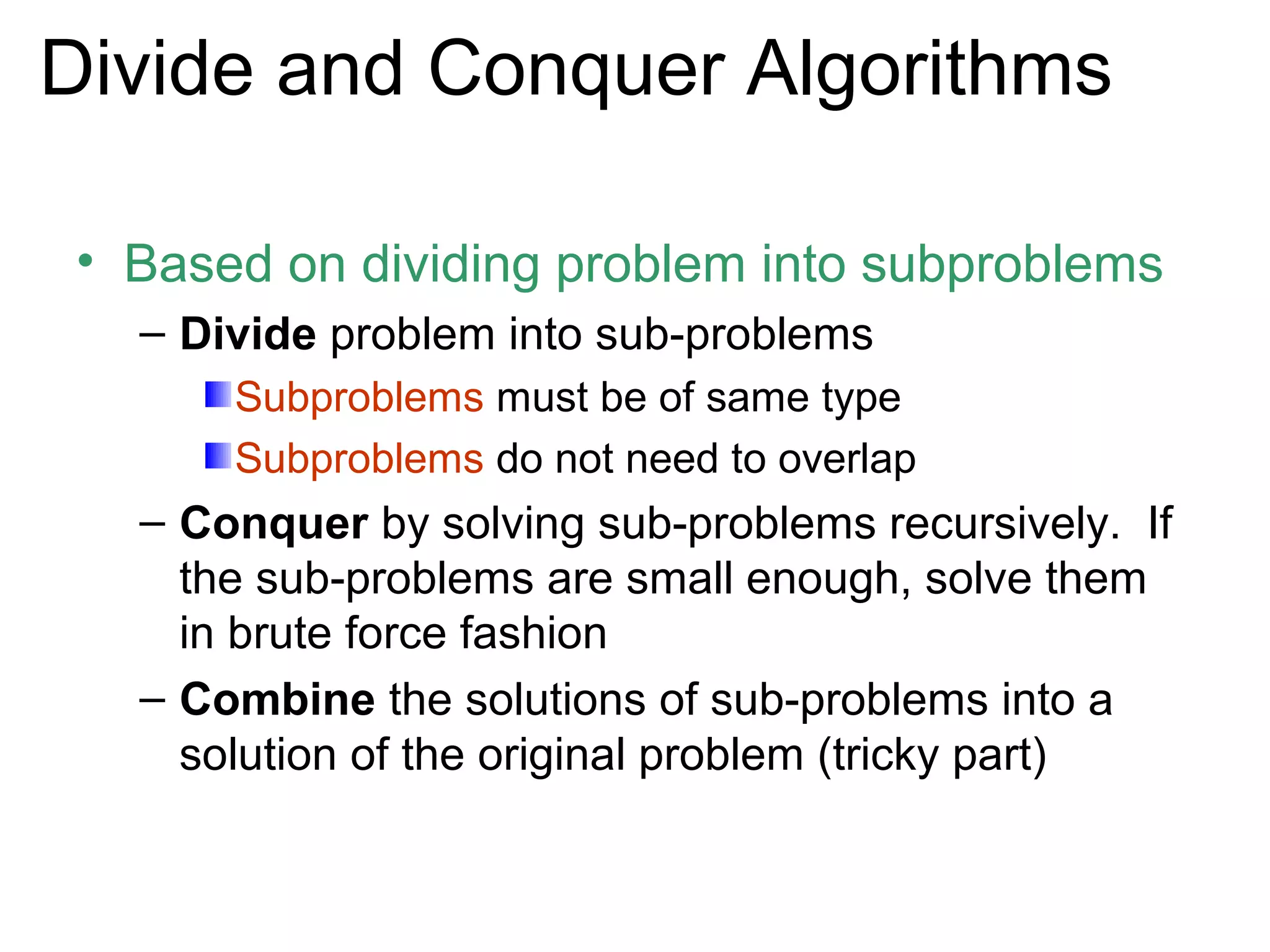
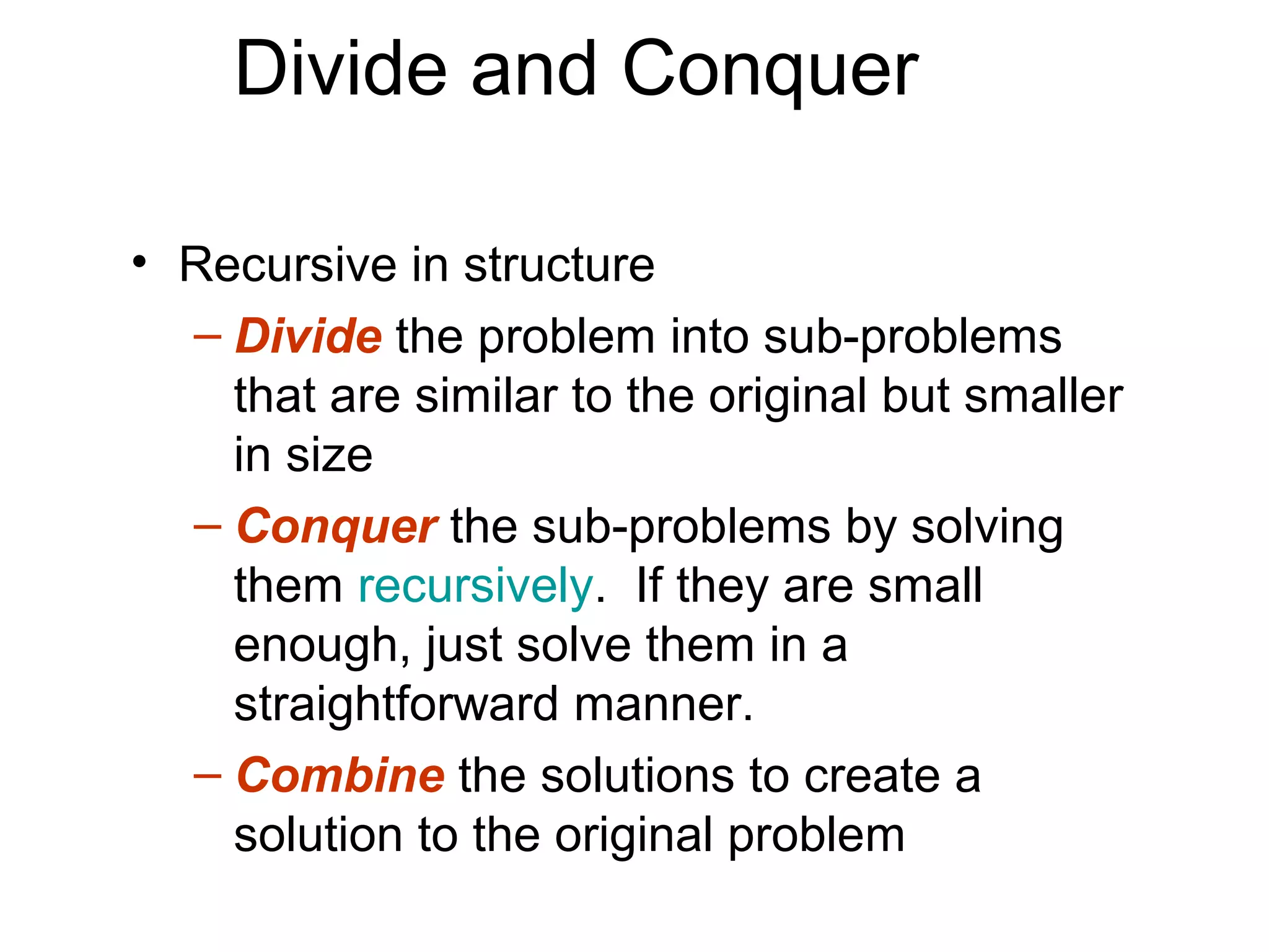
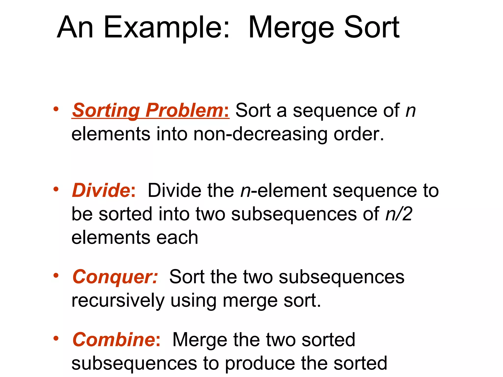
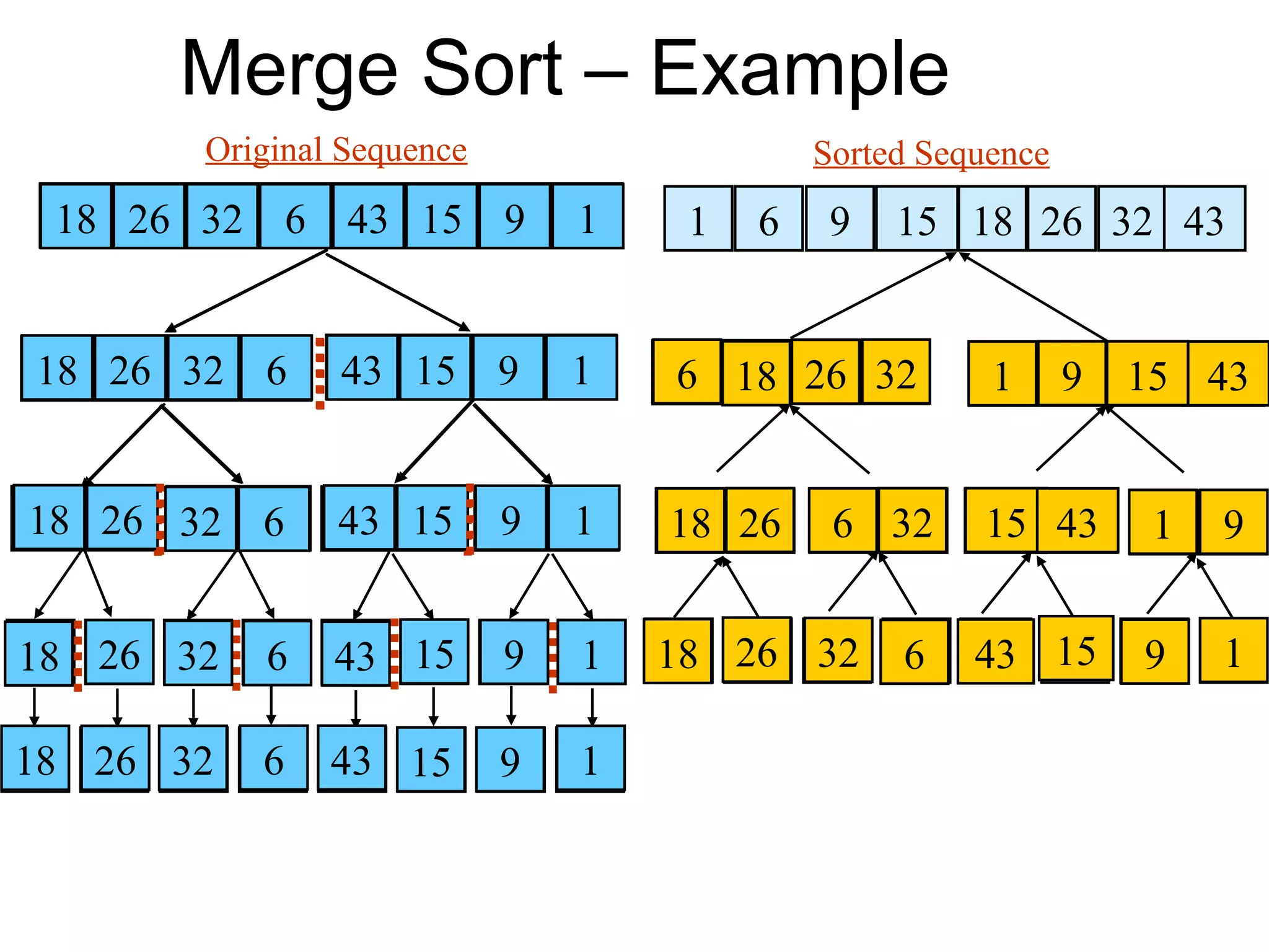
The document discusses the divide and conquer algorithm design technique. It begins by explaining the basic approach of divide and conquer which is to (1) divide the problem into subproblems, (2) conquer the subproblems by solving them recursively, and (3) combine the solutions to the subproblems into a solution for the original problem. It then provides merge sort as a specific example of a divide and conquer algorithm for sorting a sequence. It explains that merge sort divides the sequence in half recursively until individual elements remain, then combines the sorted halves back together to produce the fully sorted sequence.
Introduces Divide and Conquer as a strategy that splits problems into subproblems, recursively solves them, and combines their solutions.
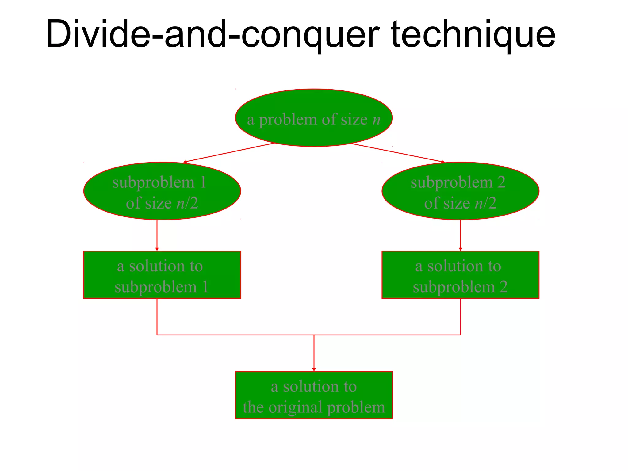
Describes the technique's process using an example of an initial problem size of n and how to solve by dividing into equal parts.
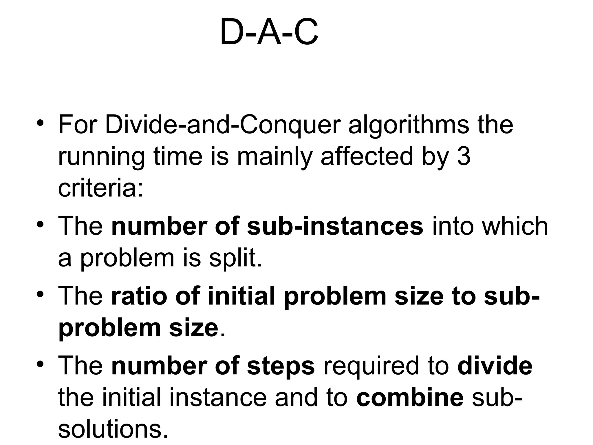
Running time of Divide and Conquer algorithms influenced by criteria like sub-instance count, size ratio, and steps for division and combination.
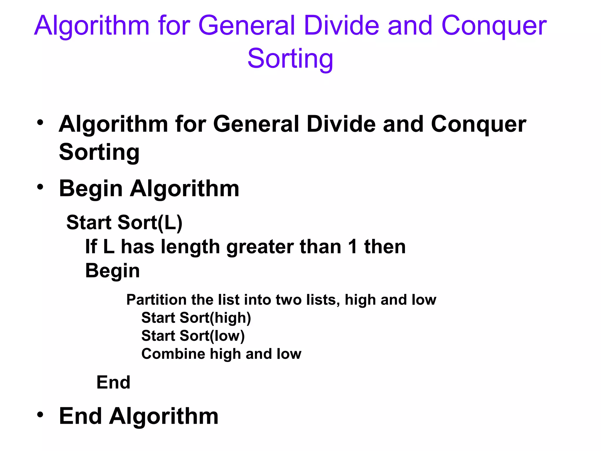
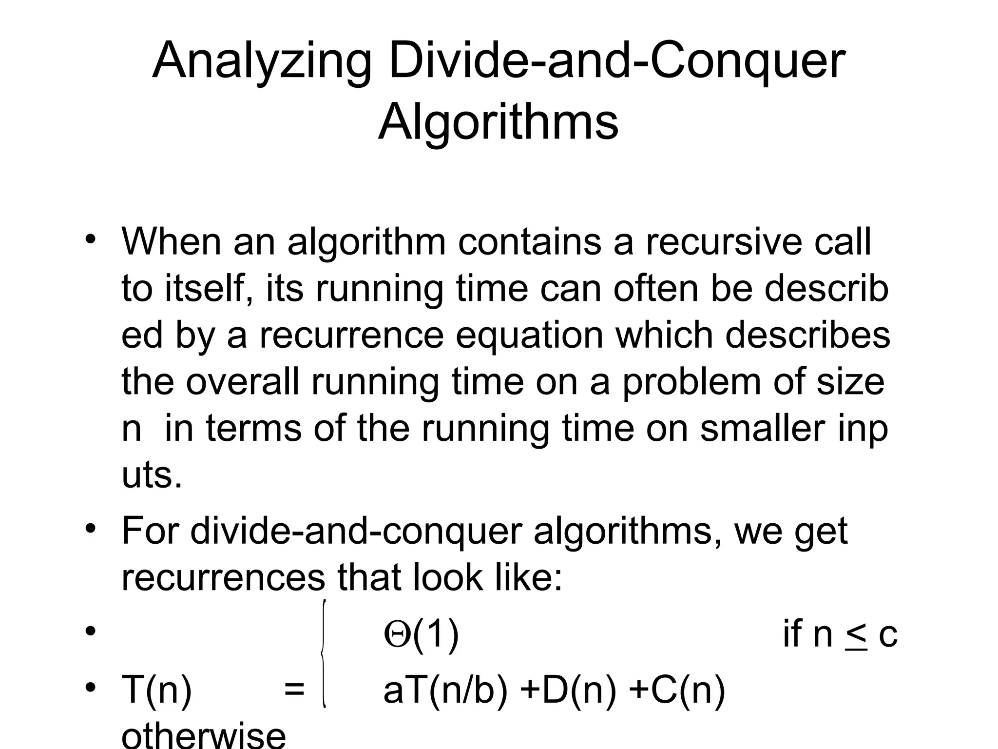
Describes an algorithm for General Divide and Conquer Sorting using recursive partitioning and analyzing its runtime through recurrence relations.
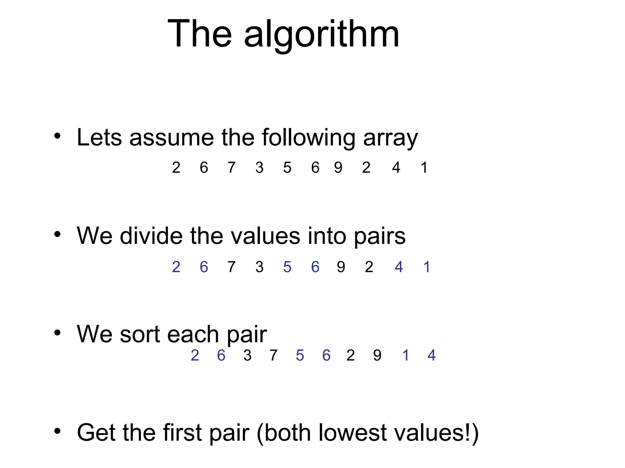
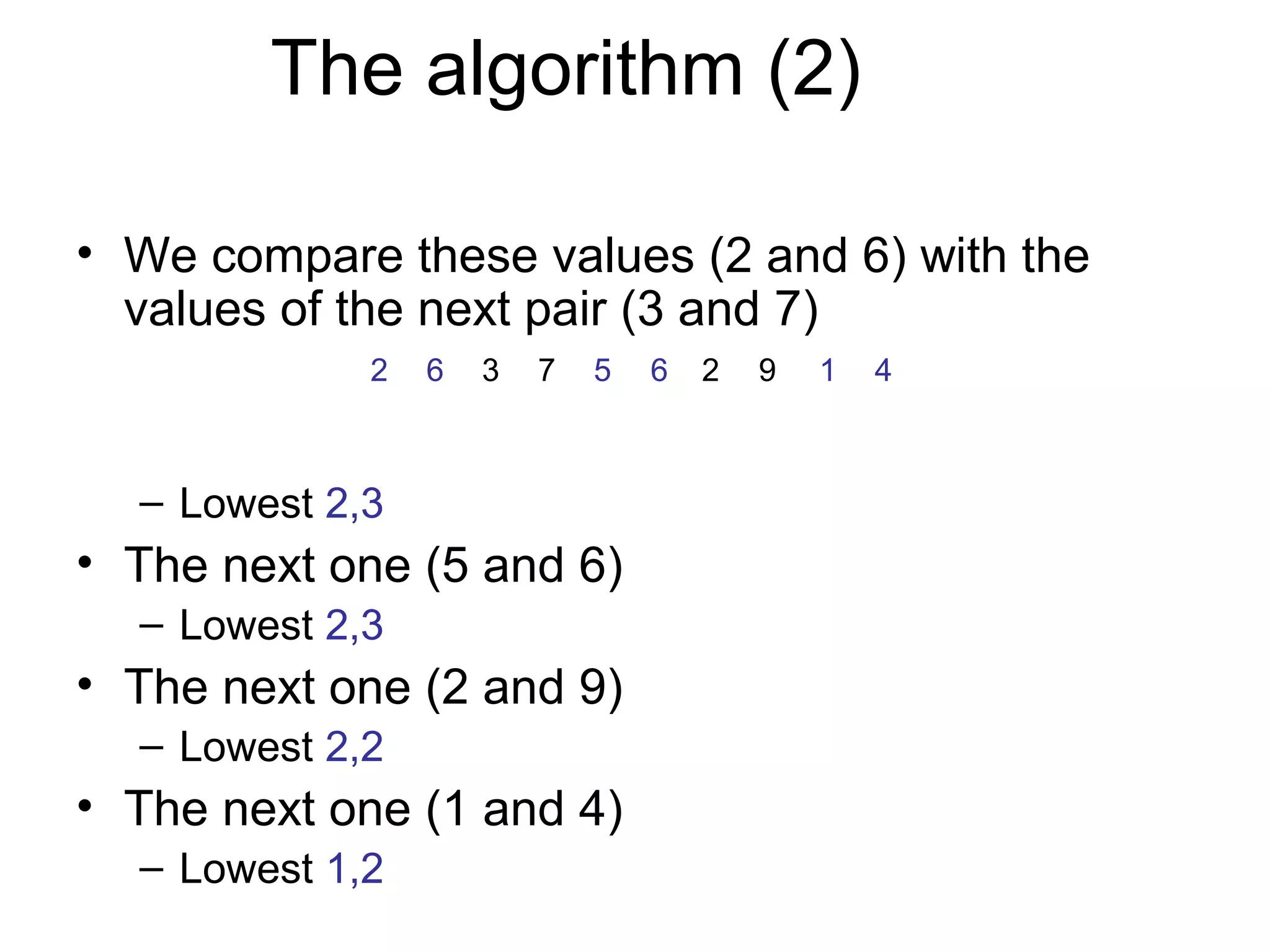
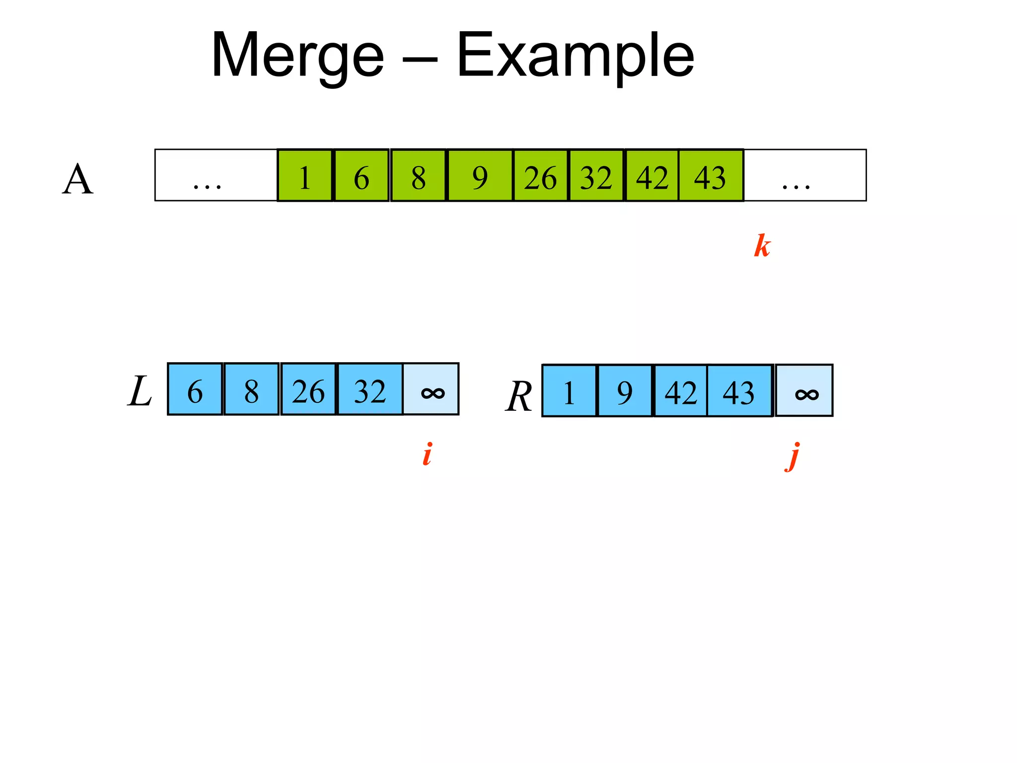
Demonstrates sorting an array based on pairs, analyzing through comparisons and highlighting the smallest elements iteratively.
Provides examples of algorithms utilizing Divide and Conquer such as Binary Search, Quick Sort, and Matrix Multiplications.
Details the Quicksort algorithm, its divide, conquer, and combine phases, and compares it with Merge Sort.
Presents the pseudocode for Quicksort and walks through an example highlighting the partitioning and correctness of the algorithm.
Explains the correctness of partitioning in Quicksort through loop invariants and how the algorithm maintains conditions during execution.
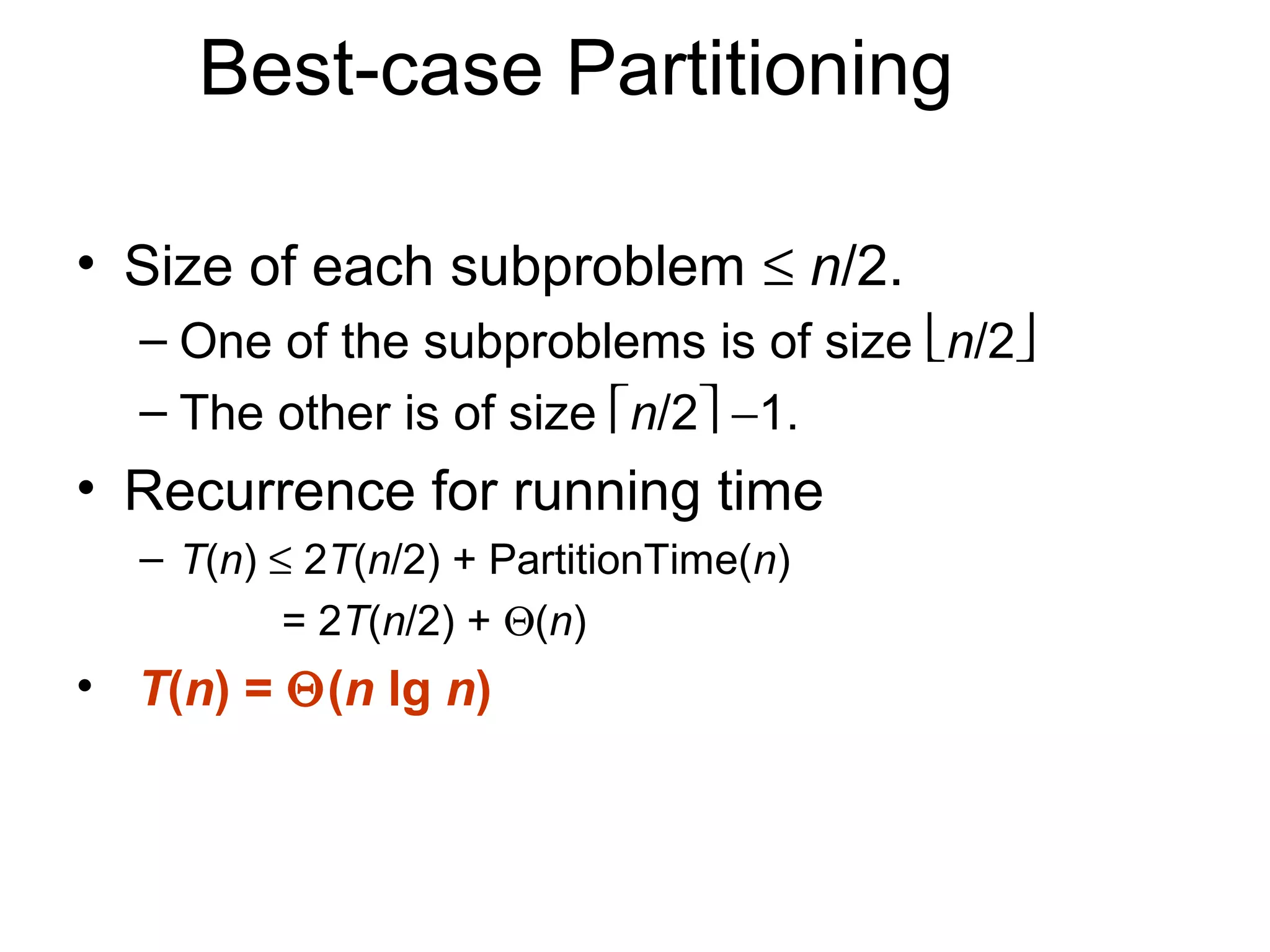
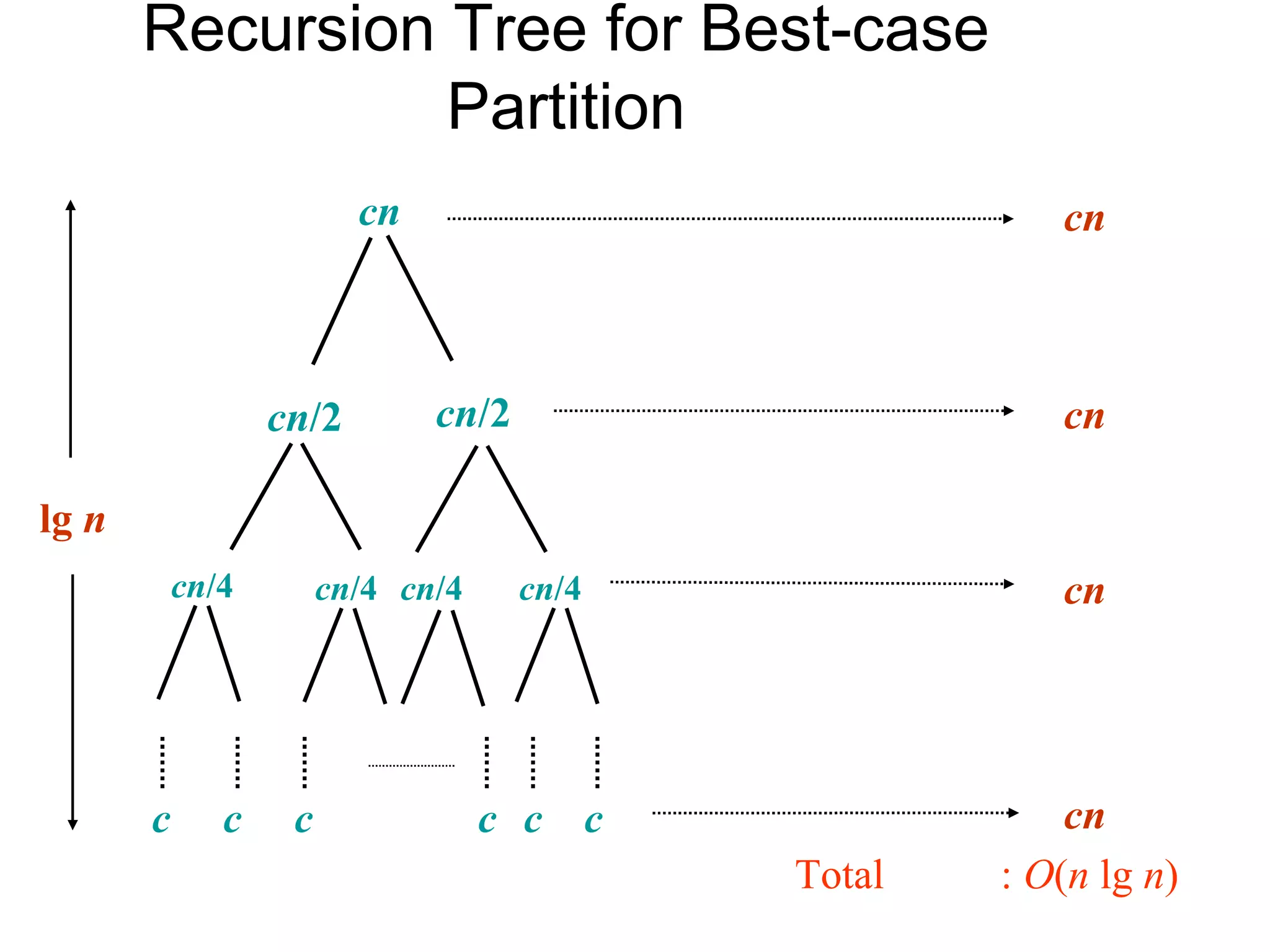
Analyzes the running time complexity for both worst-case and best-case scenarios in the Quicksort algorithm.
Summarizes the significance of Divide and Conquer as a powerful algorithm design technique and its efficiency in solving problems.
Introduces Merge Sort following the Divide and Conquer strategy. Details the process of dividing, sorting, and merging subsequences.
Outlines the implementation of Merge Sort and the merging procedure with examples illustrating the sorting steps and correctness.
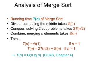
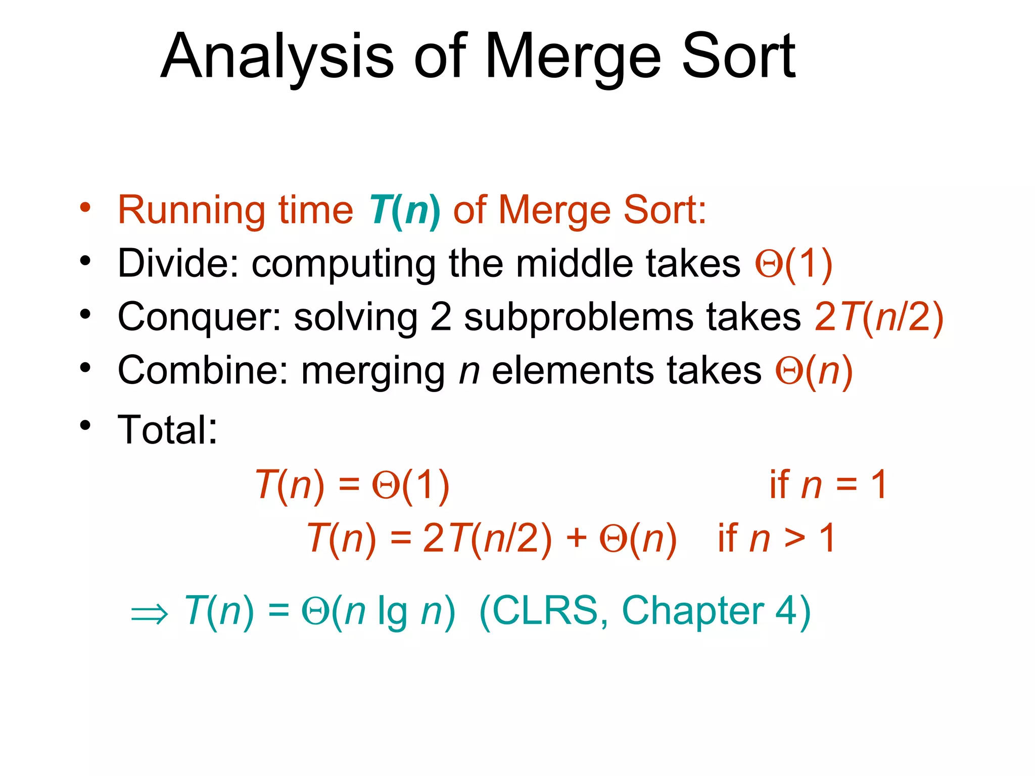
Discusses the correctness of the Merge procedure and its analysis, establishing its running time as Θ(n log n) and explaining steps involved.


