Downloaded 616 times
![How to merge two sorted sequences We have two subarrays A[p..q] and A[q+1..r] in sorted order. Merge sort algorithm merges them to form a single sorted subarray that replaces the current subarray A[p..r]](https://image.slidesharecdn.com/algorithmppt82/85/Algorithm-ppt-4-320.jpg)
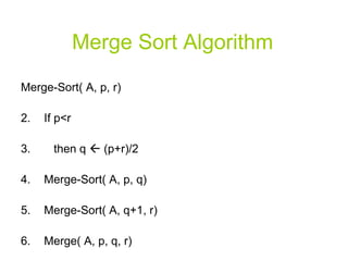
![Merging Algorithm Merge( A, p, q, r) n1 q – p + 1 n2 r – q Create arrays L[1..n1+1] and R[1..n2+1]](https://image.slidesharecdn.com/algorithmppt82/85/Algorithm-ppt-5-320.jpg)
![Merging Algorithm 4. For i 1 to n1 do L[i] A[p + i -1] 6. For j 1 to n2 do R[j] A[q + j]](https://image.slidesharecdn.com/algorithmppt82/85/Algorithm-ppt-6-320.jpg)
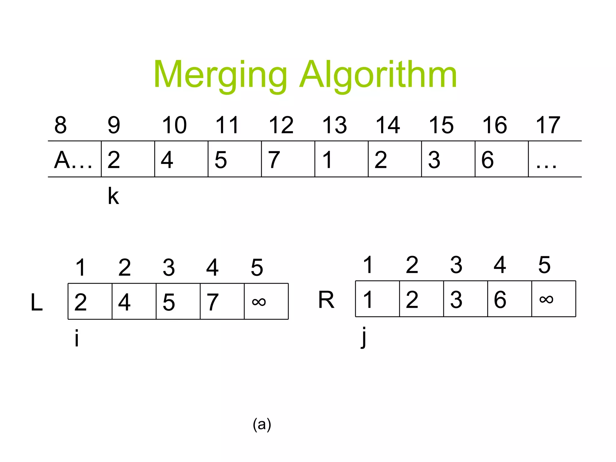
![Merging Algorithm 8. L[n1 + 1] ∞ 9. R[n2 + 1] ∞ 10. i 1 11. j 1](https://image.slidesharecdn.com/algorithmppt82/85/Algorithm-ppt-7-320.jpg)
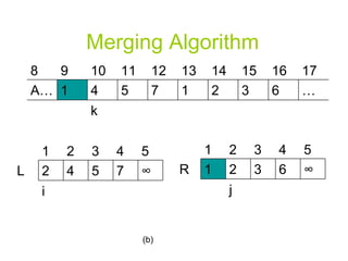
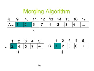
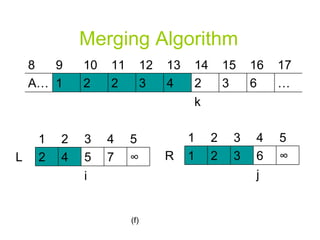
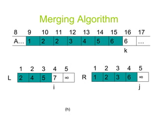
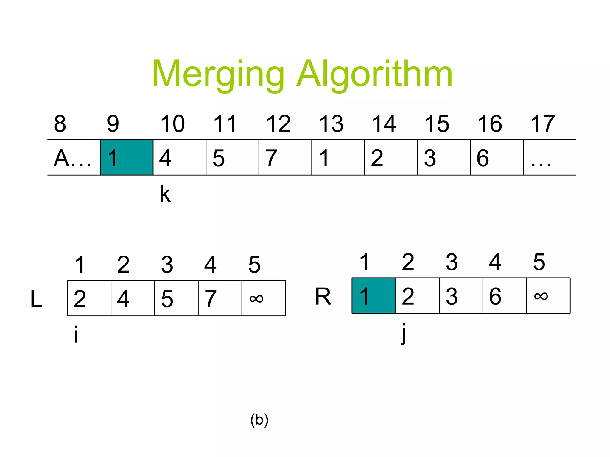
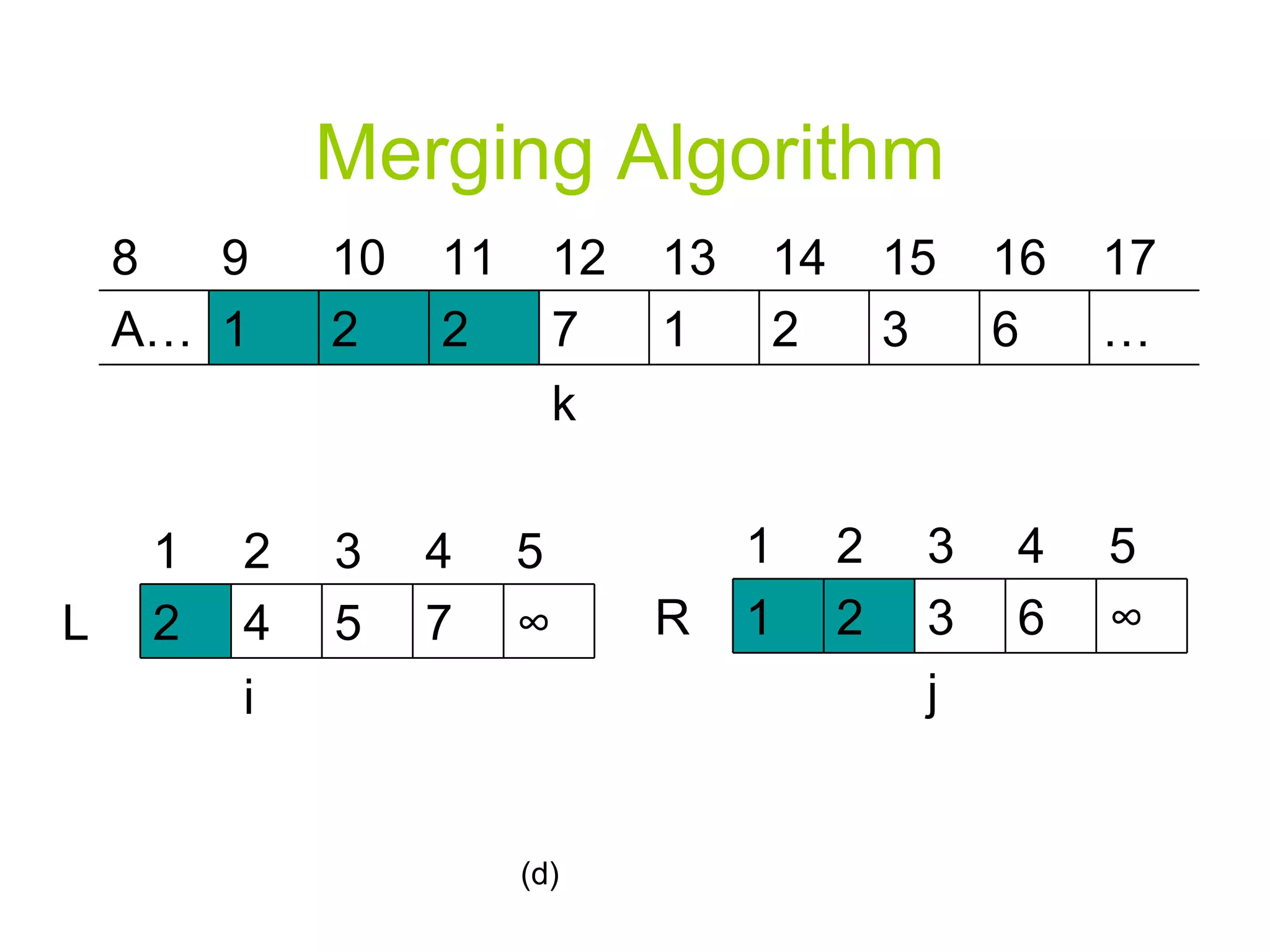
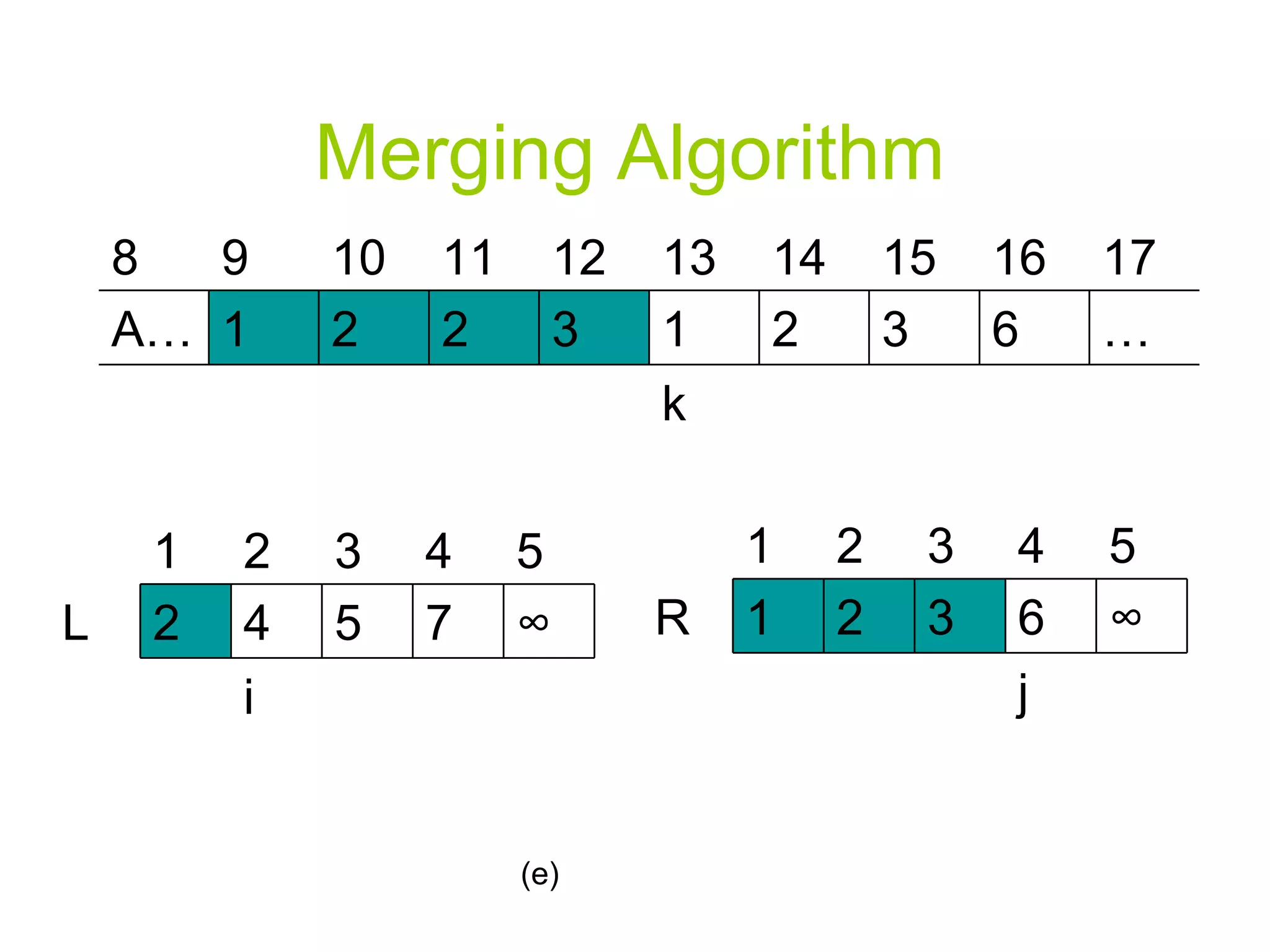
![Merging Algorithm 12. For k p to r 13. Do if L[i] <= R[j] 14. Then A[k] L[i] i=i+1 else A[k] R[j] j=j+1](https://image.slidesharecdn.com/algorithmppt82/85/Algorithm-ppt-8-320.jpg)
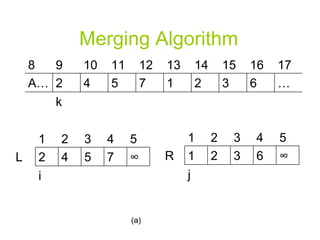


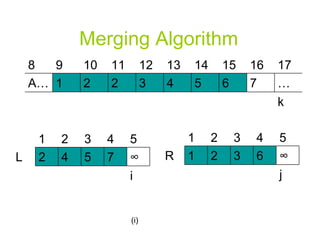


![How to merge two sorted sequences We have two subarrays A[p..q] and A[q+1..r] in sorted order. Merge sort algorithm merges them to form a single sorted subarray that replaces the current subarray A[p..r]](https://image.slidesharecdn.com/algorithmppt82/75/Algorithm-ppt-4-2048.jpg)
![Merging Algorithm Merge( A, p, q, r) n1 q – p + 1 n2 r – q Create arrays L[1..n1+1] and R[1..n2+1]](https://image.slidesharecdn.com/algorithmppt82/75/Algorithm-ppt-5-2048.jpg)
![Merging Algorithm 4. For i 1 to n1 do L[i] A[p + i -1] 6. For j 1 to n2 do R[j] A[q + j]](https://image.slidesharecdn.com/algorithmppt82/75/Algorithm-ppt-6-2048.jpg)
![Merging Algorithm 8. L[n1 + 1] ∞ 9. R[n2 + 1] ∞ 10. i 1 11. j 1](https://image.slidesharecdn.com/algorithmppt82/75/Algorithm-ppt-7-2048.jpg)
![Merging Algorithm 12. For k p to r 13. Do if L[i] <= R[j] 14. Then A[k] L[i] i=i+1 else A[k] R[j] j=j+1](https://image.slidesharecdn.com/algorithmppt82/75/Algorithm-ppt-8-2048.jpg)

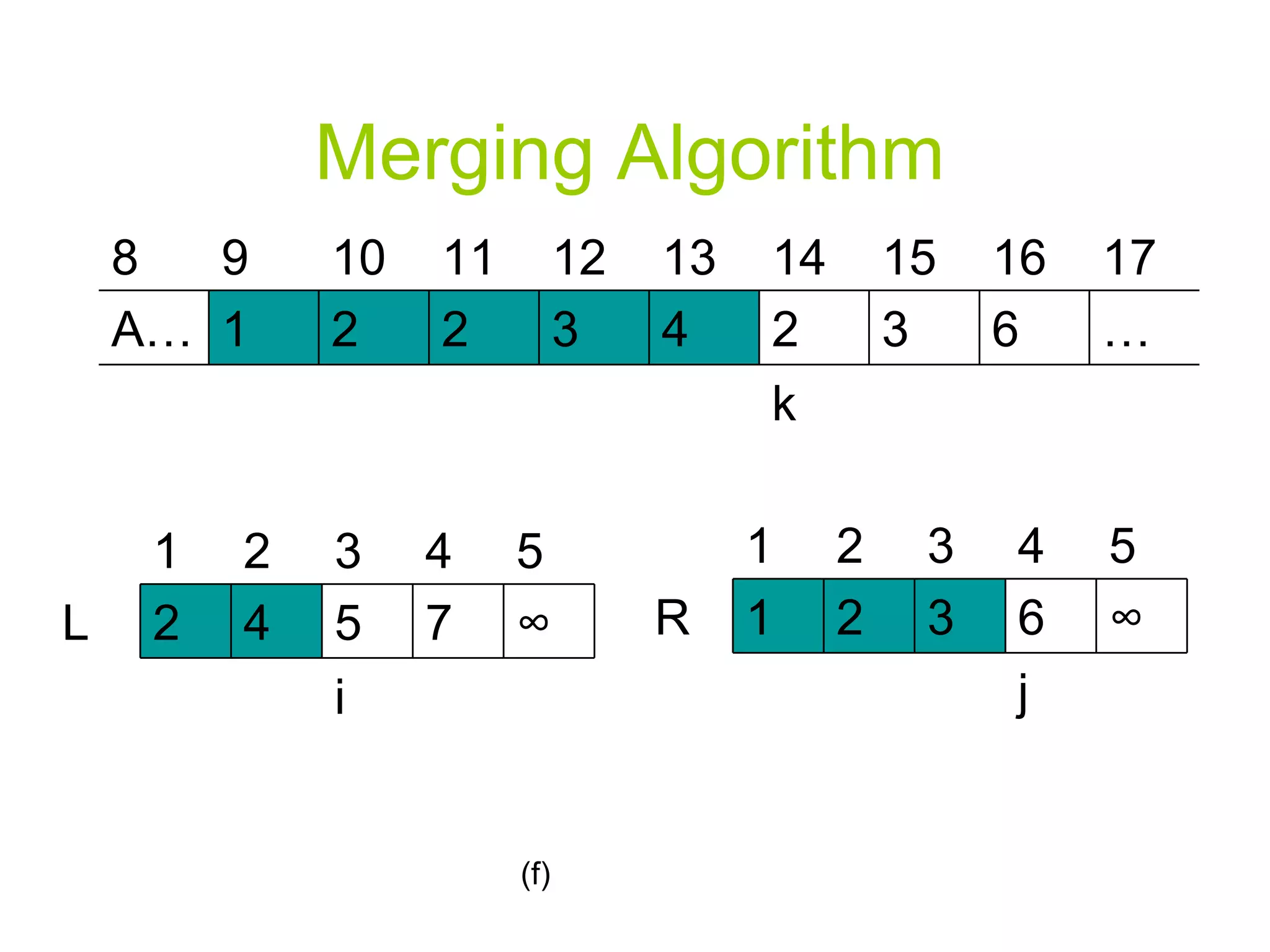
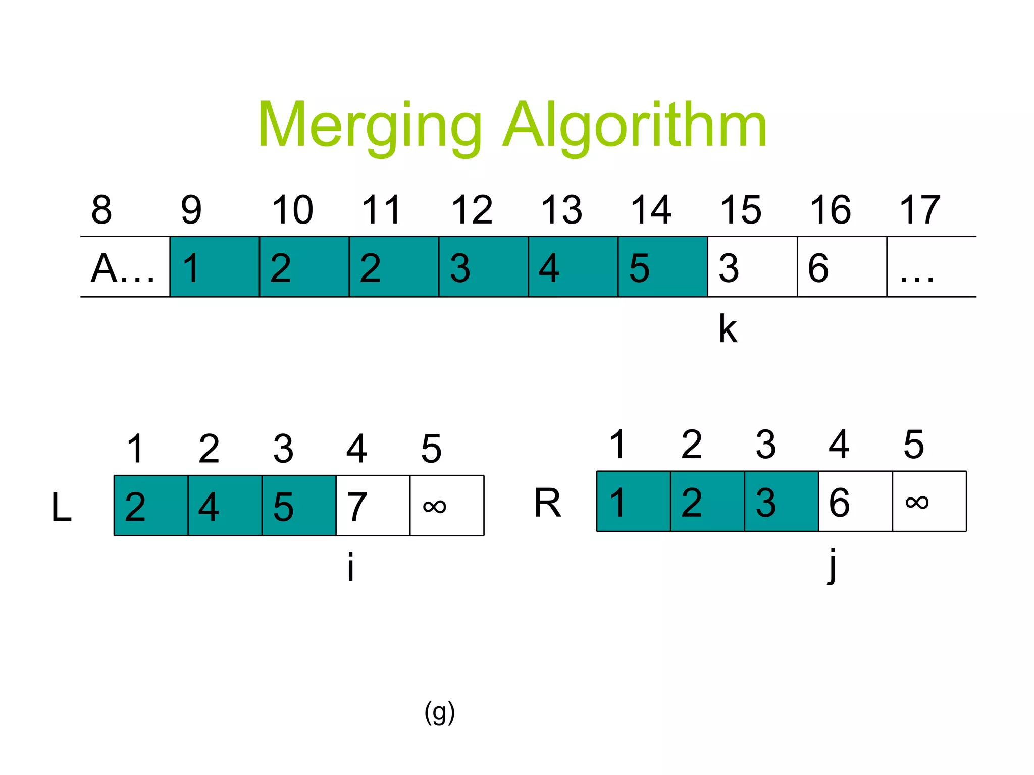
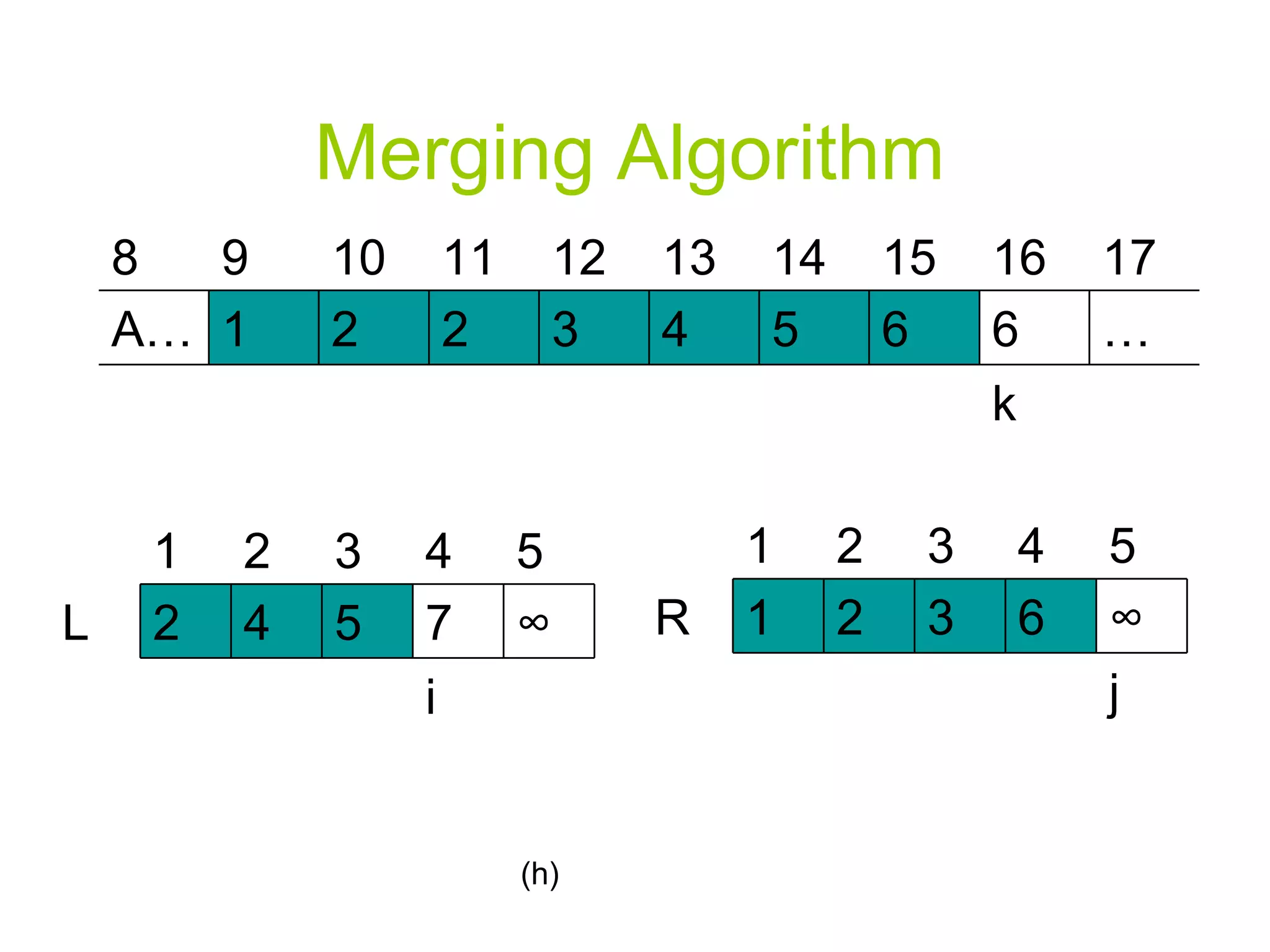
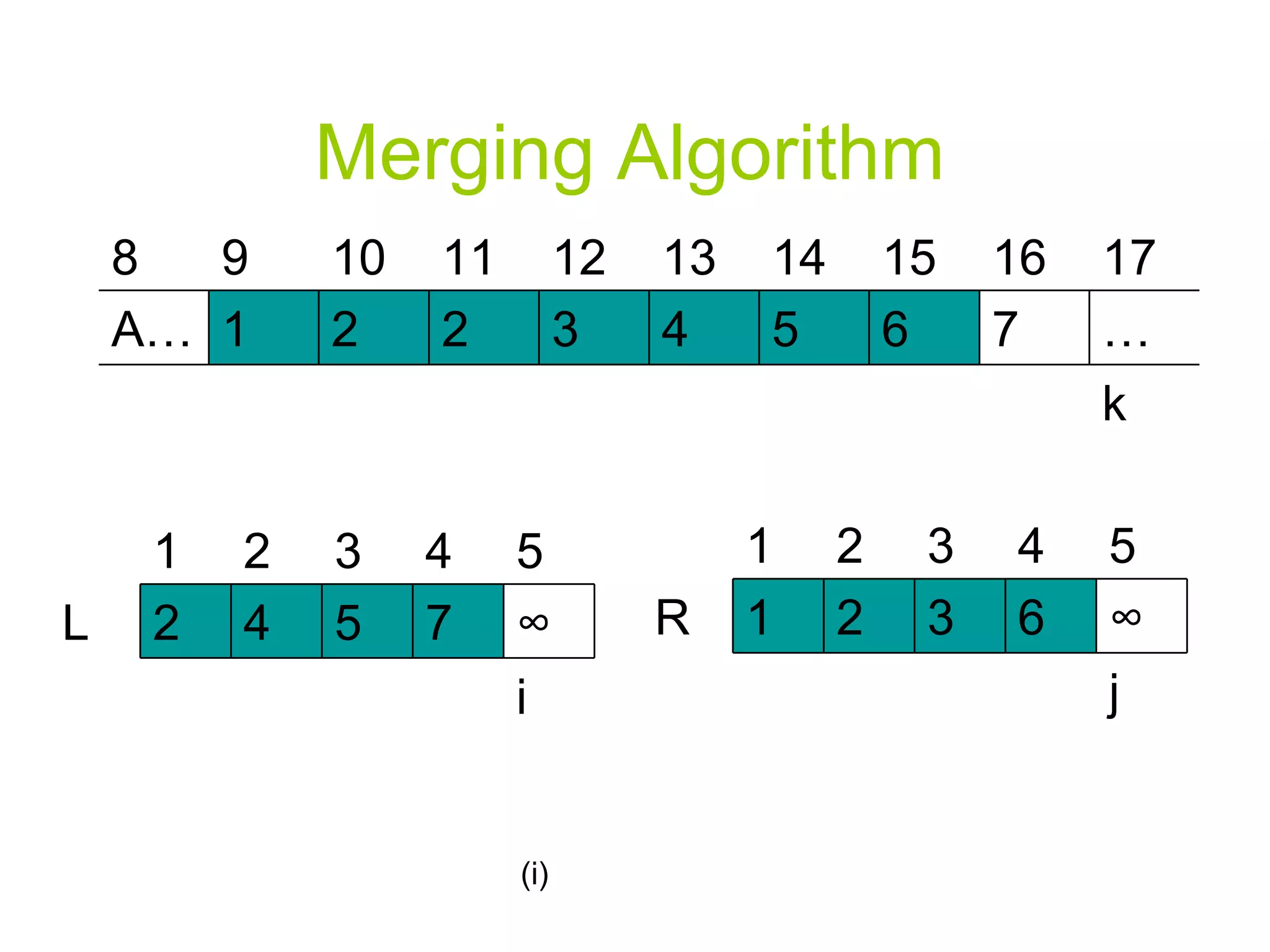
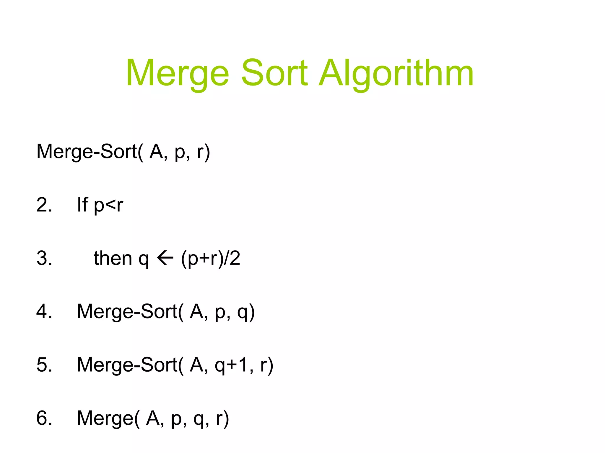
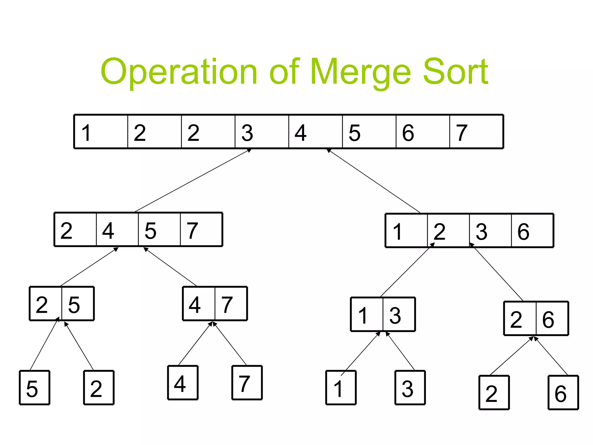
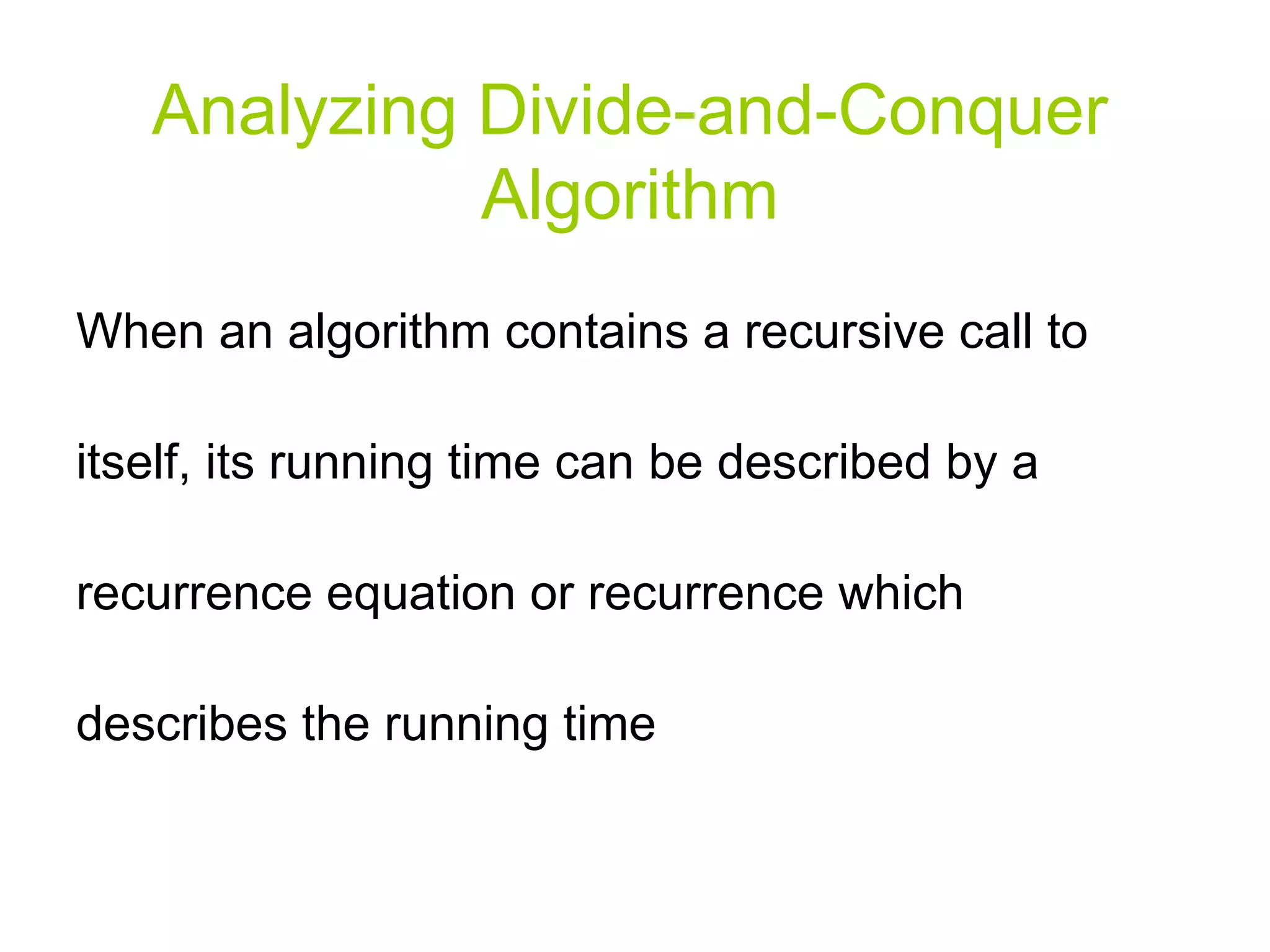
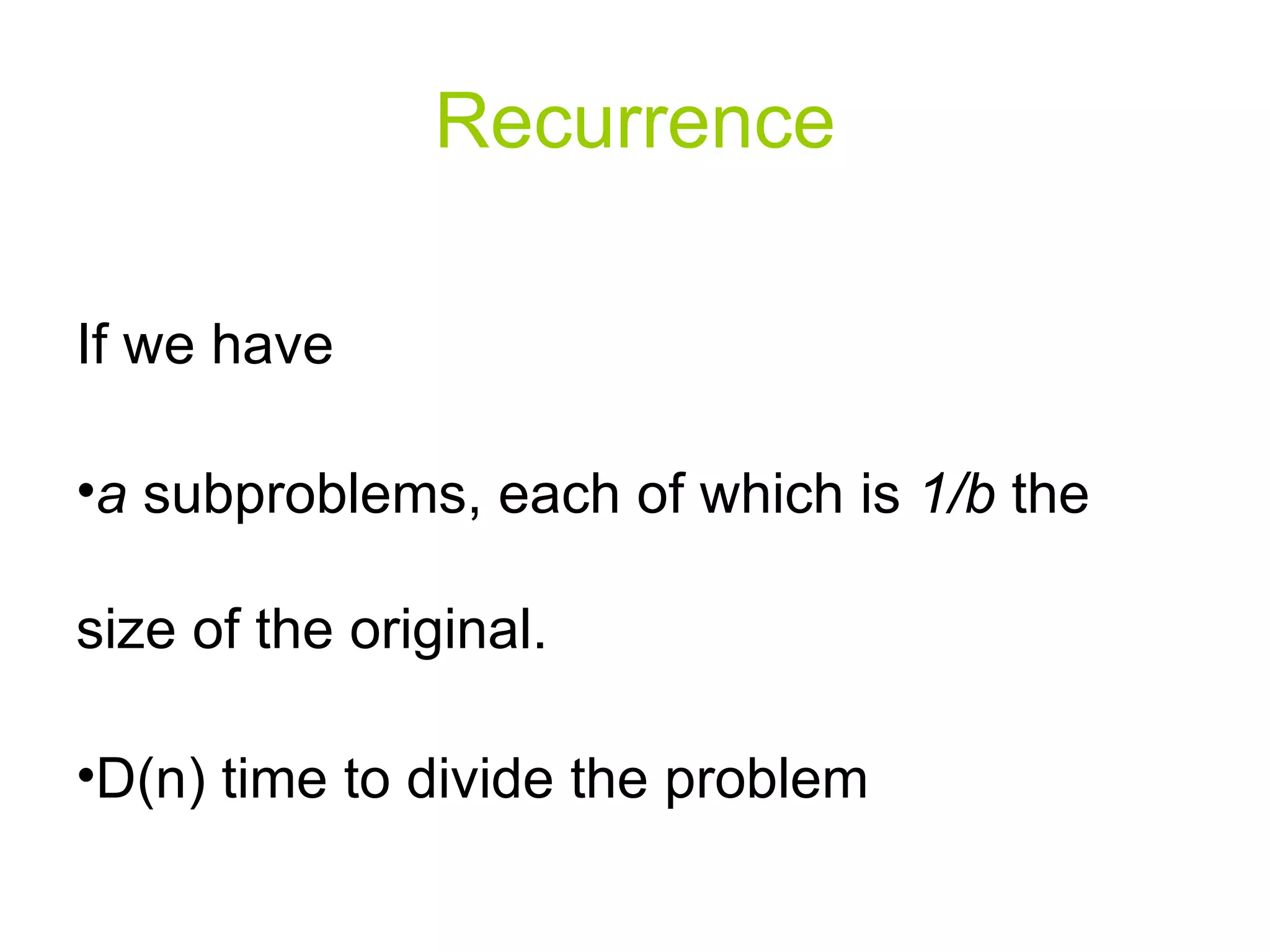
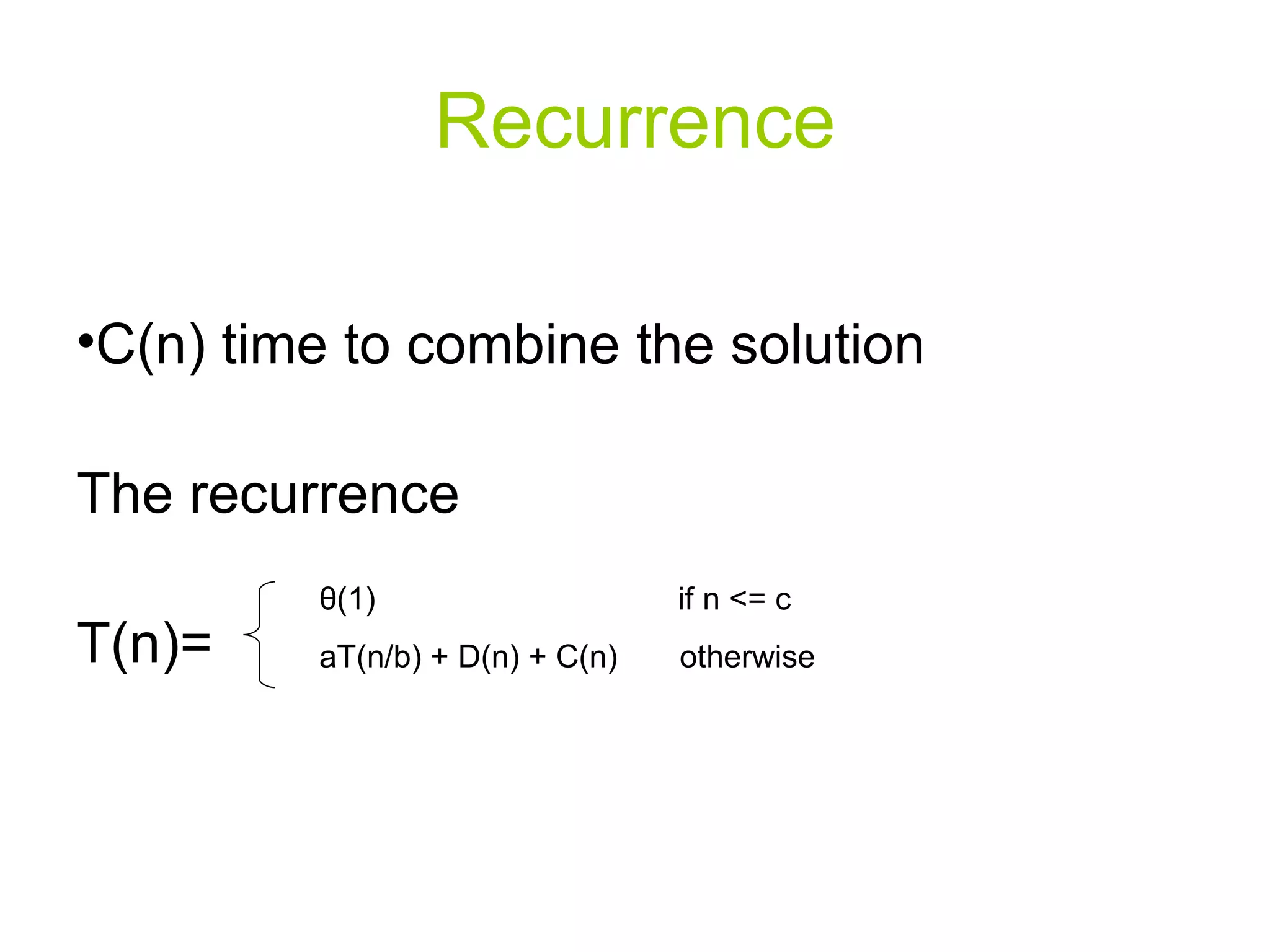
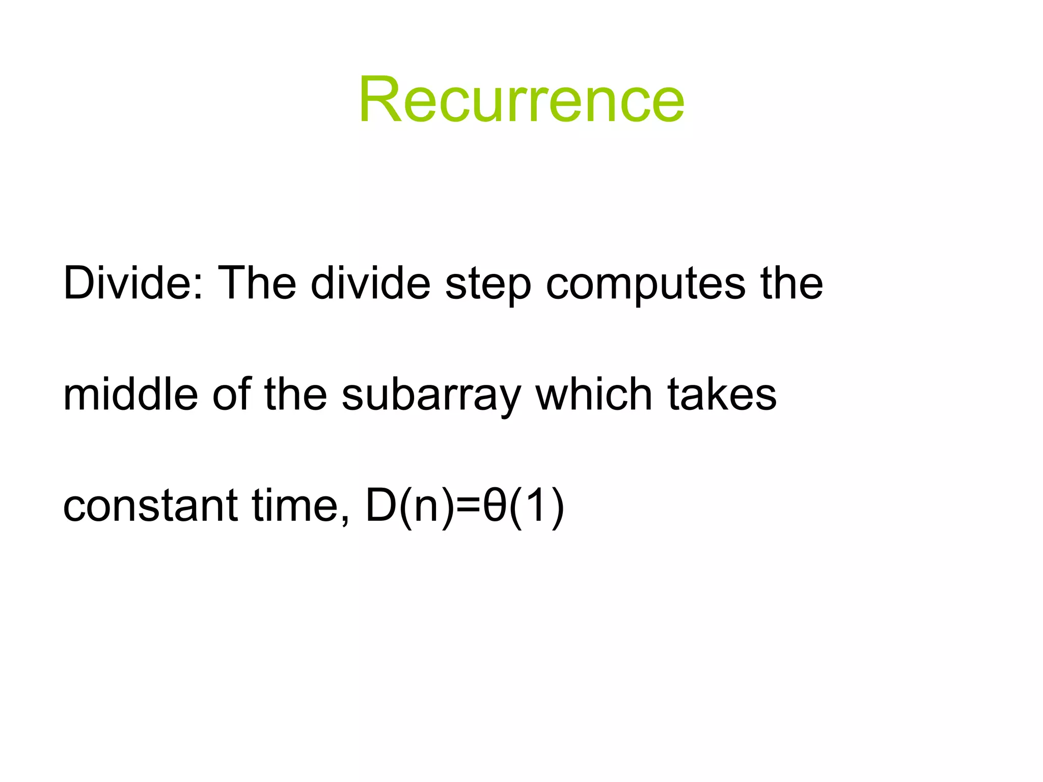
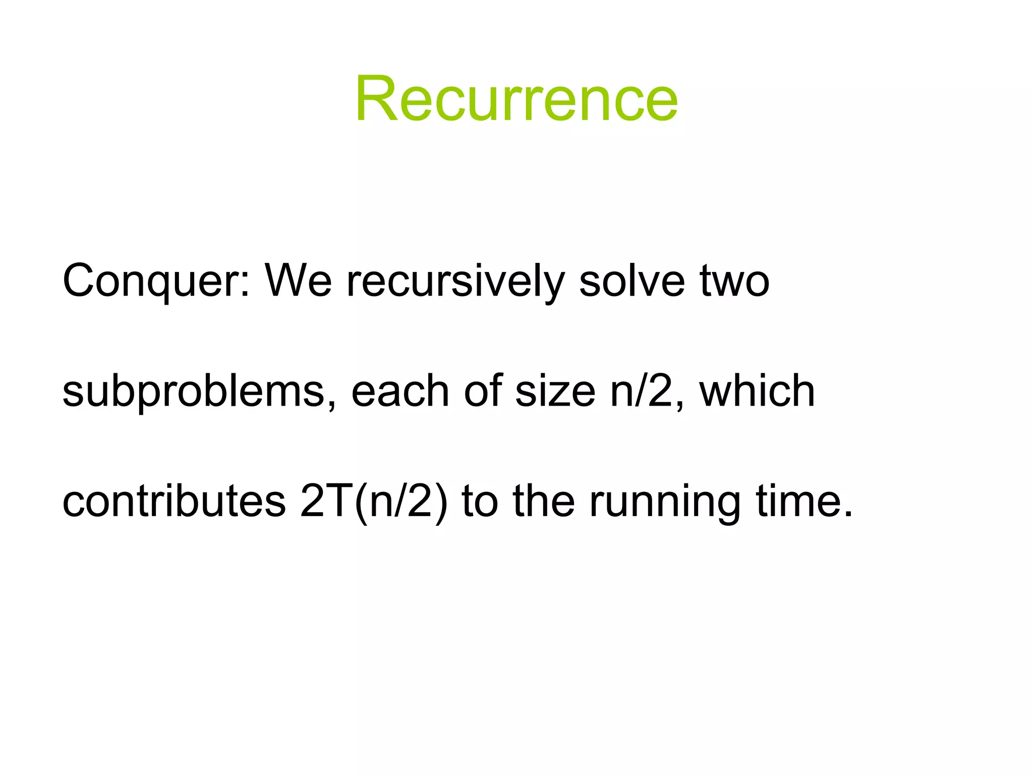
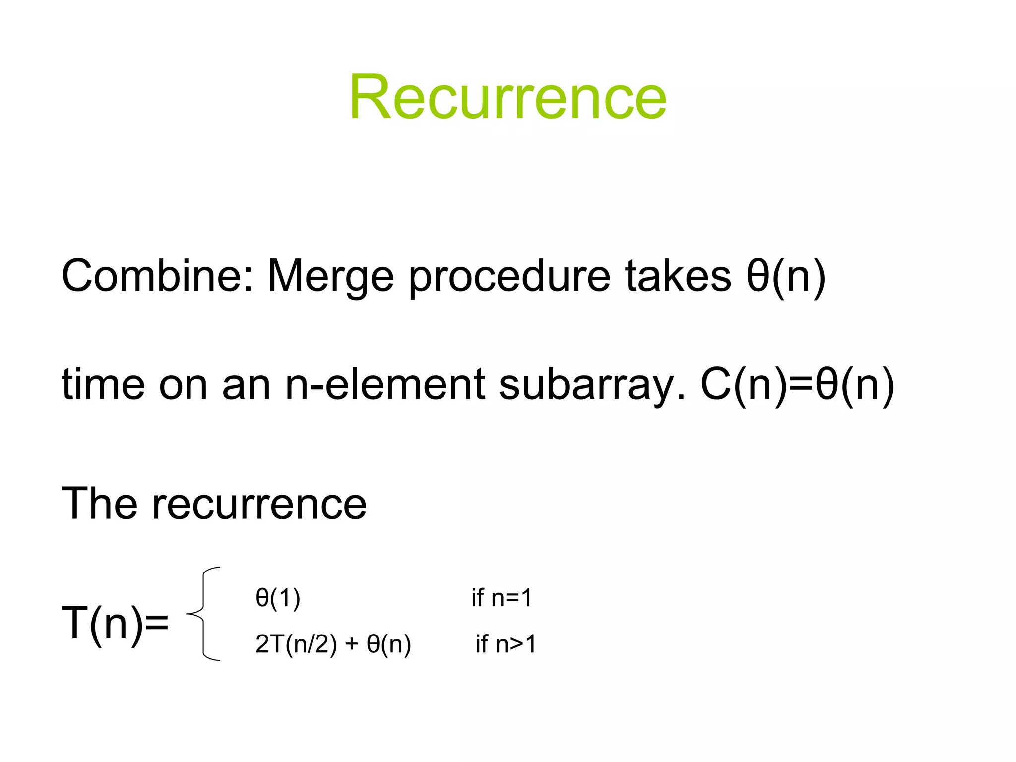
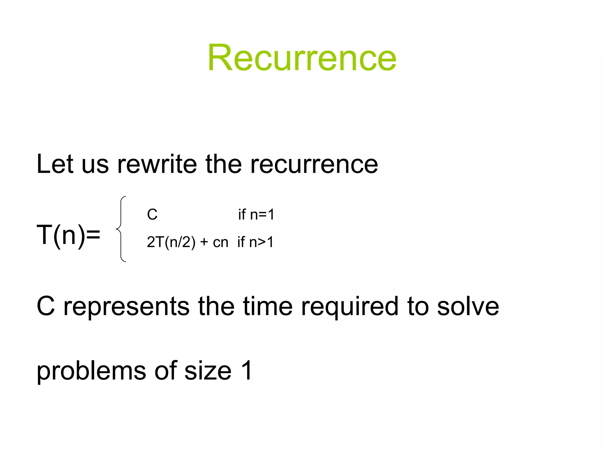
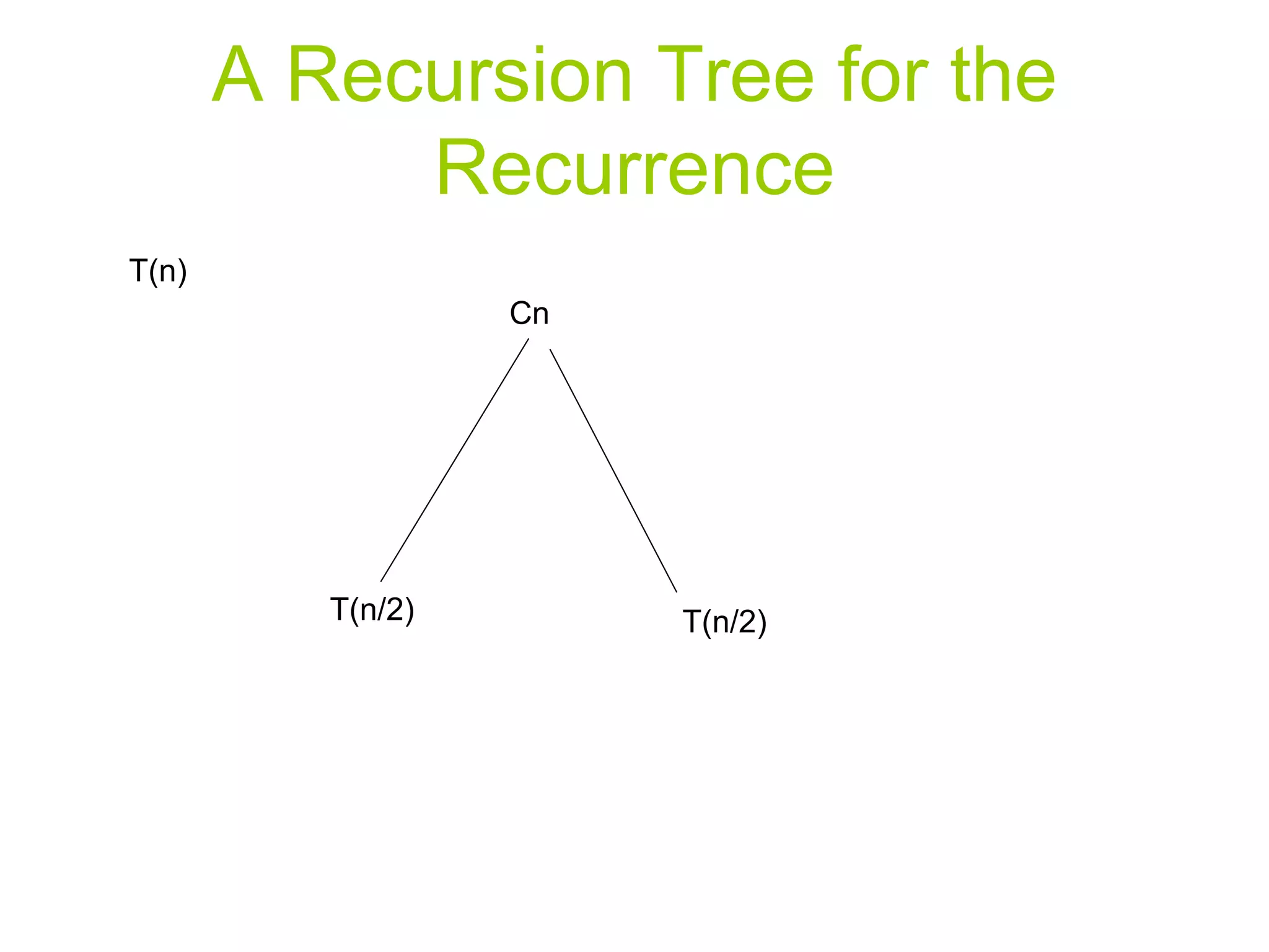
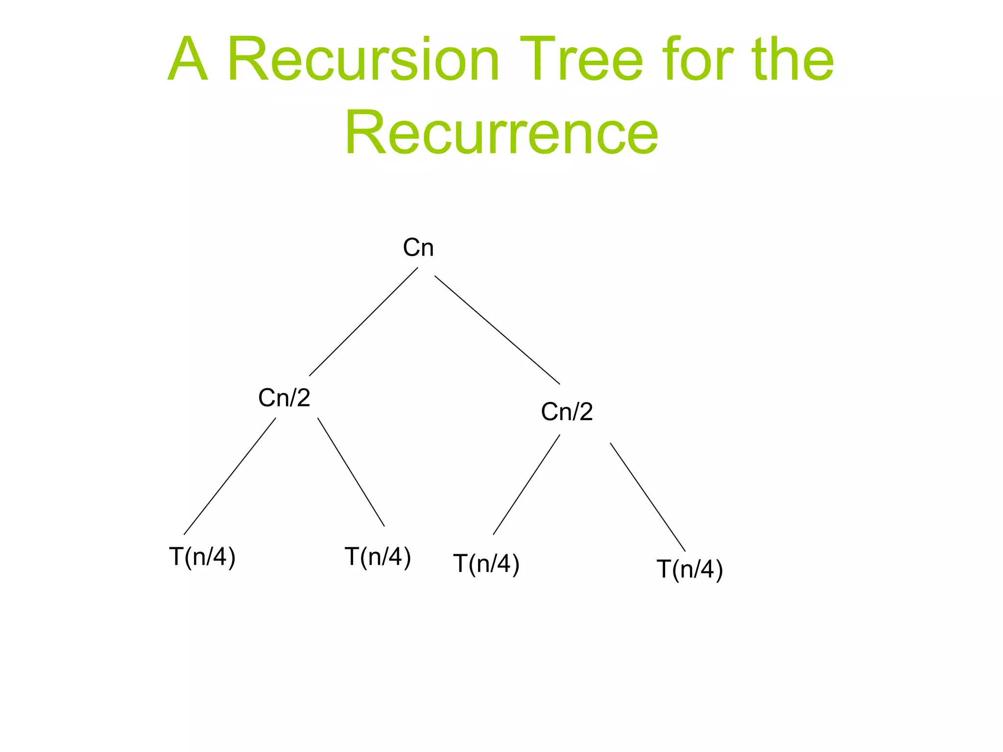
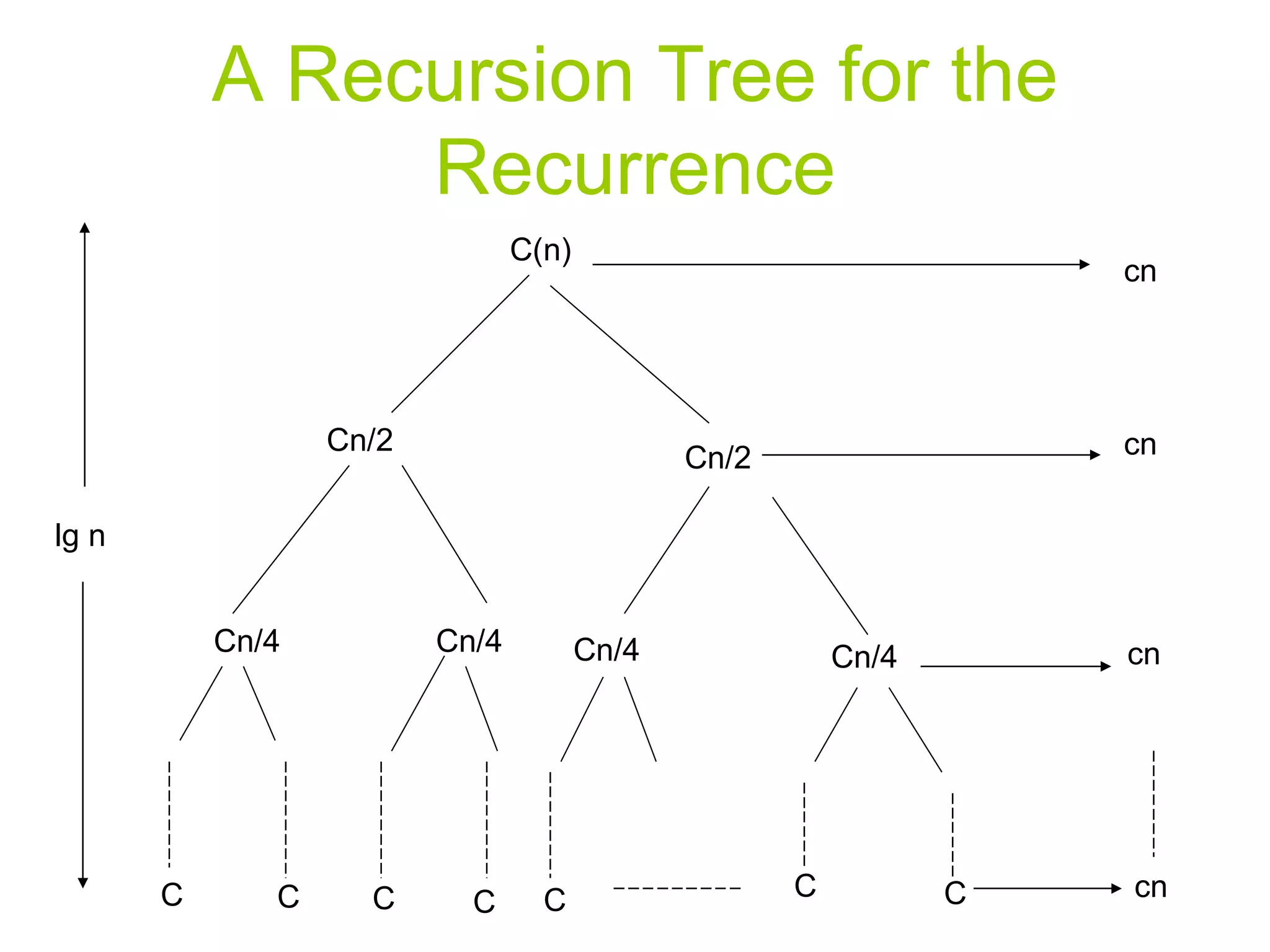
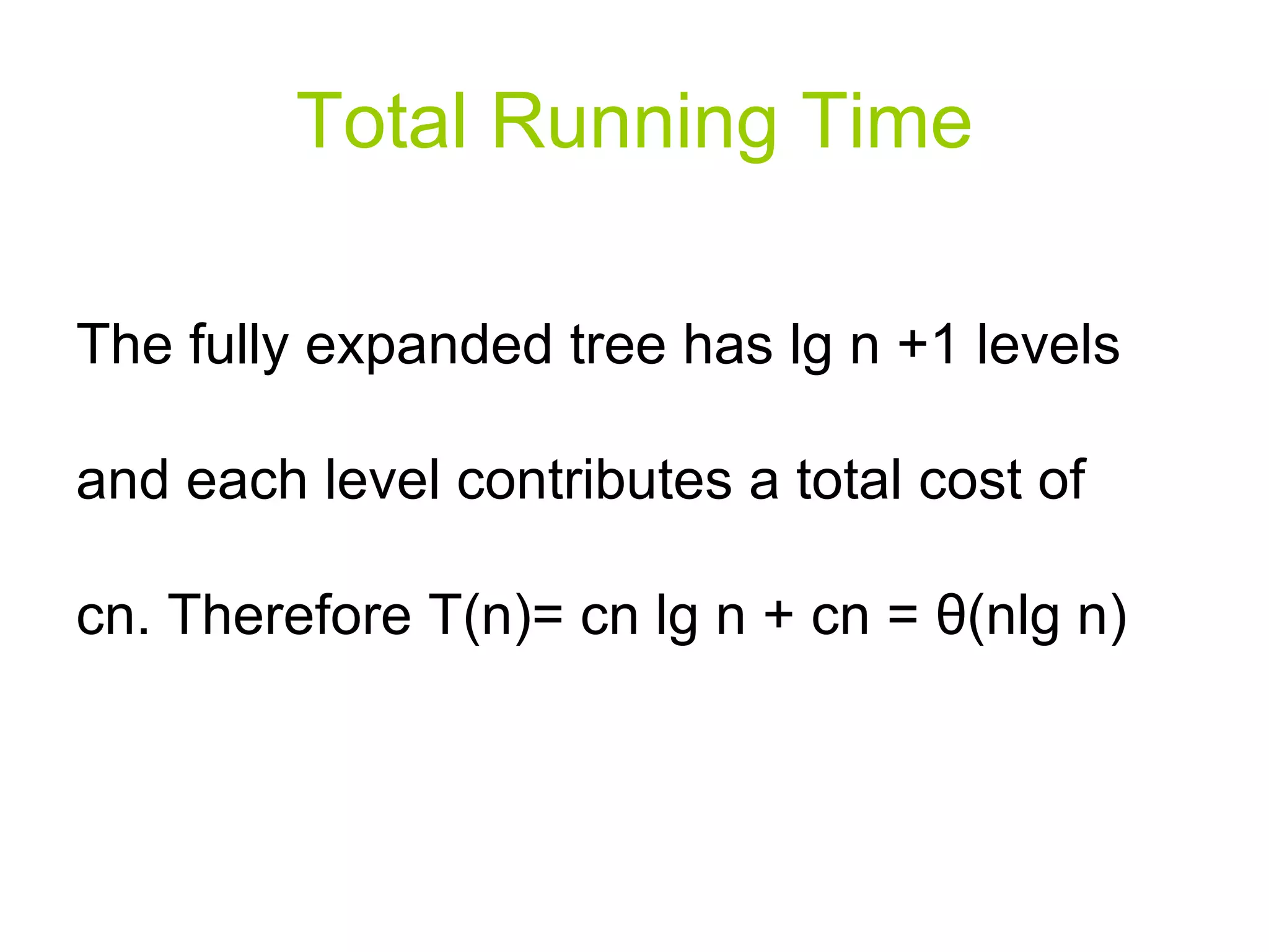
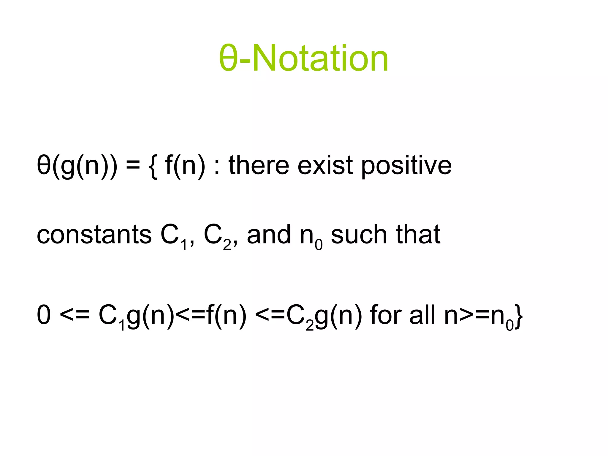
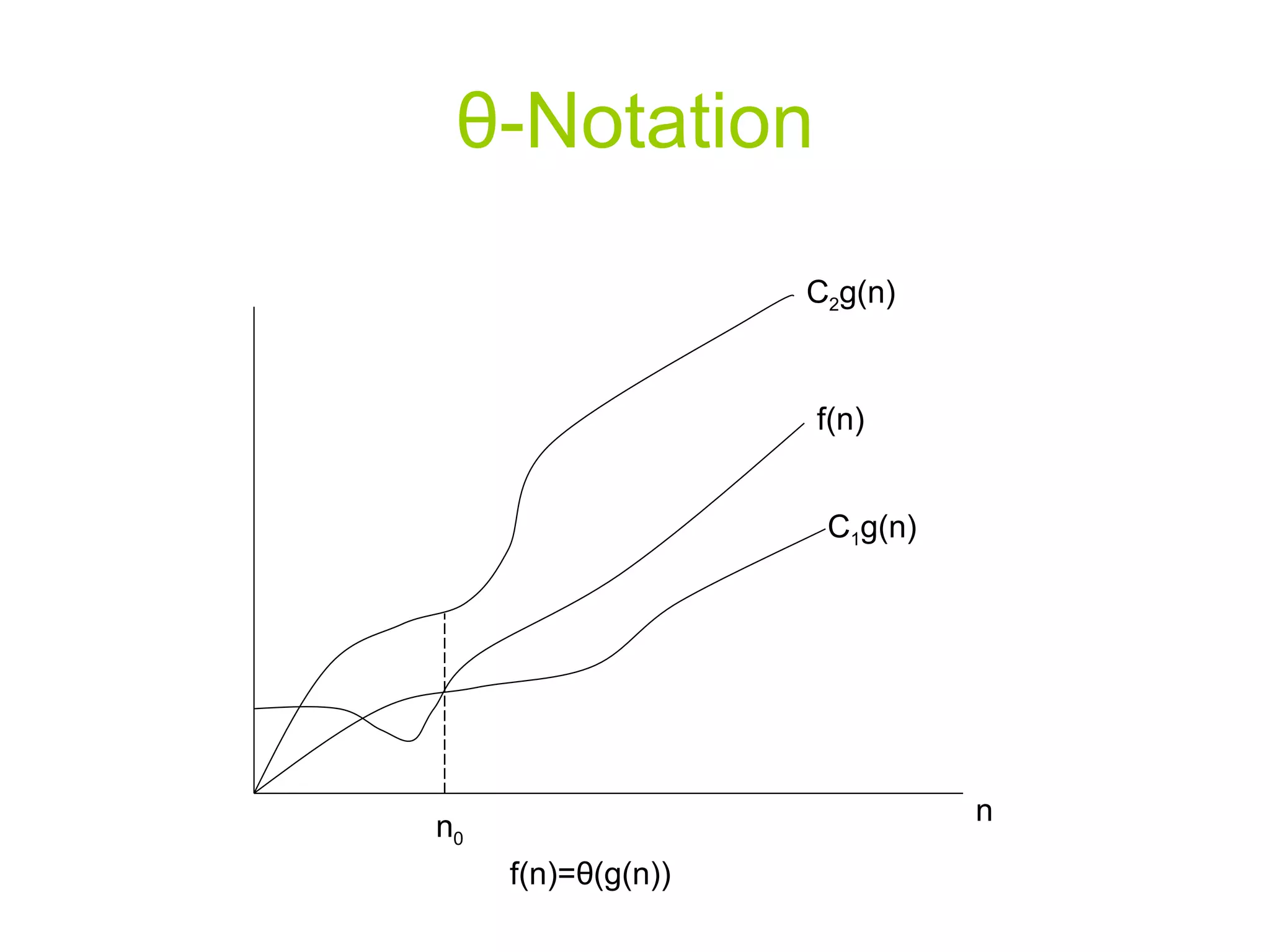
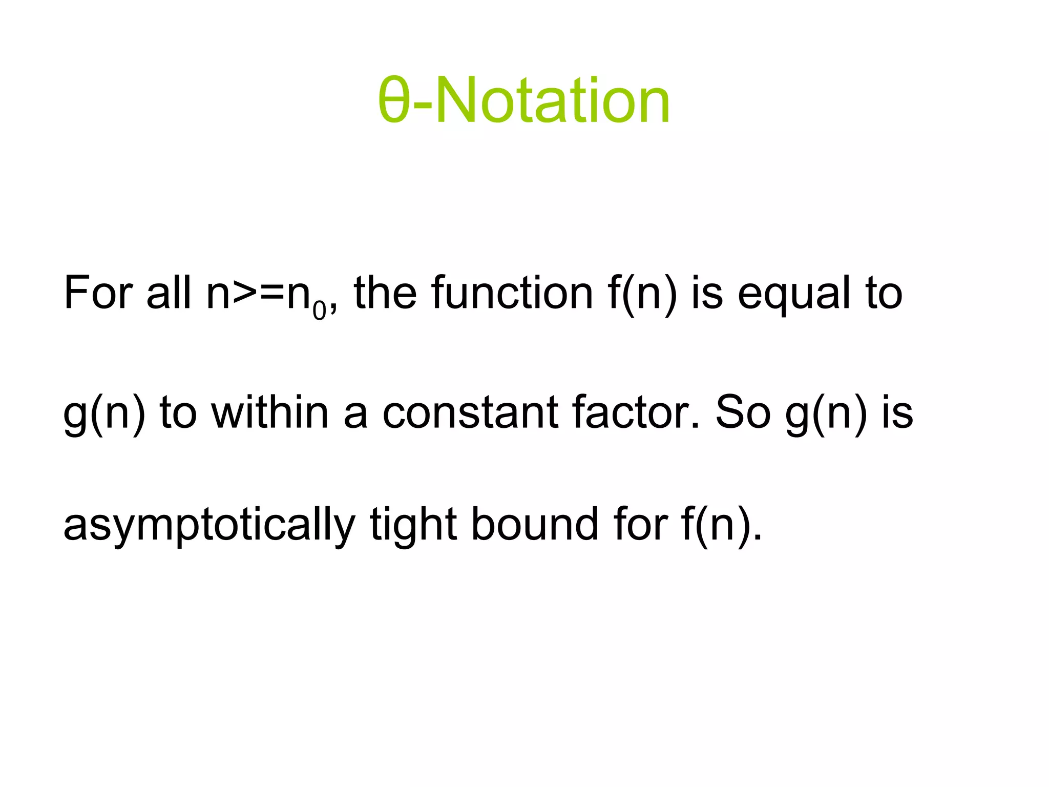

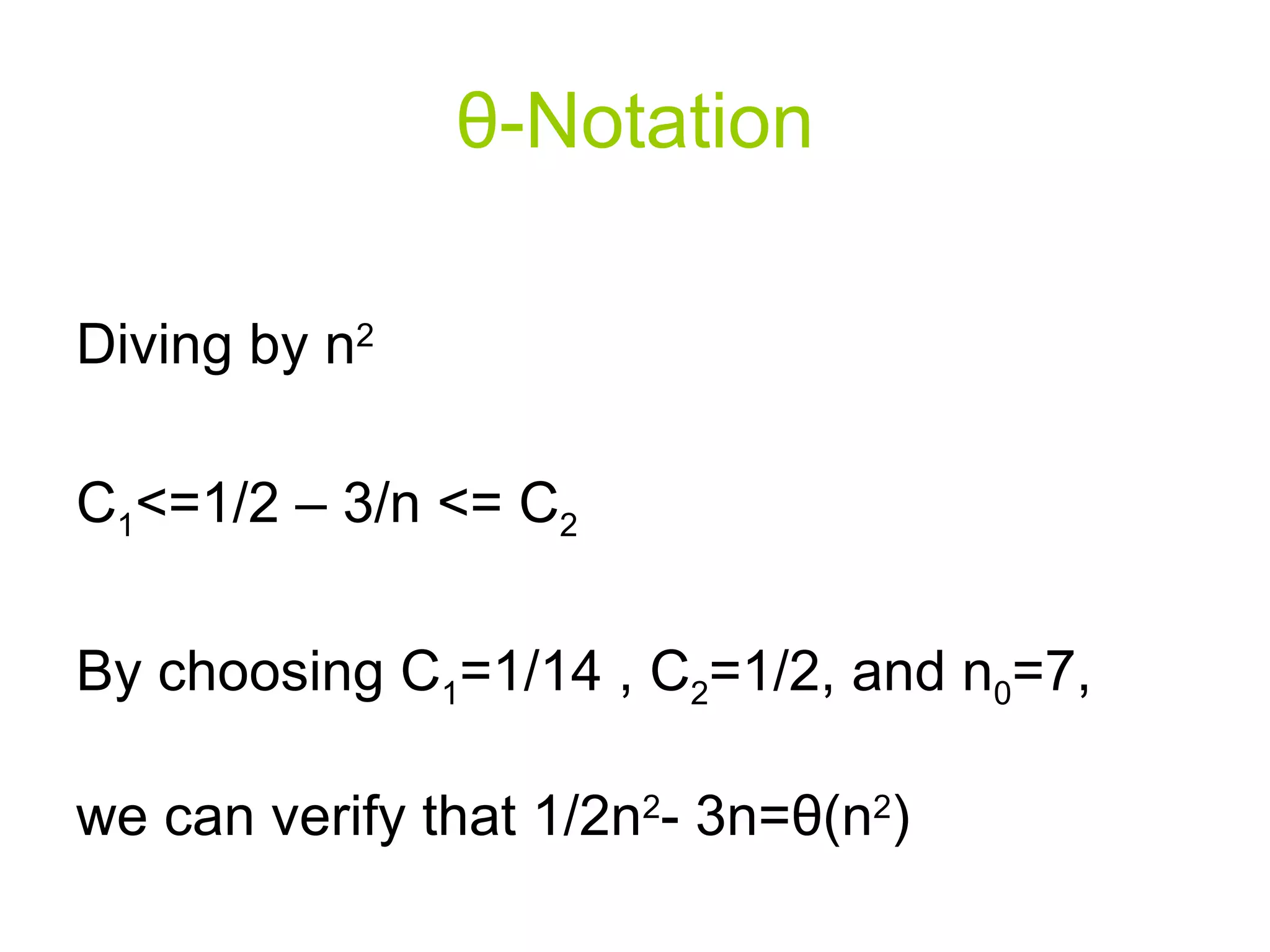

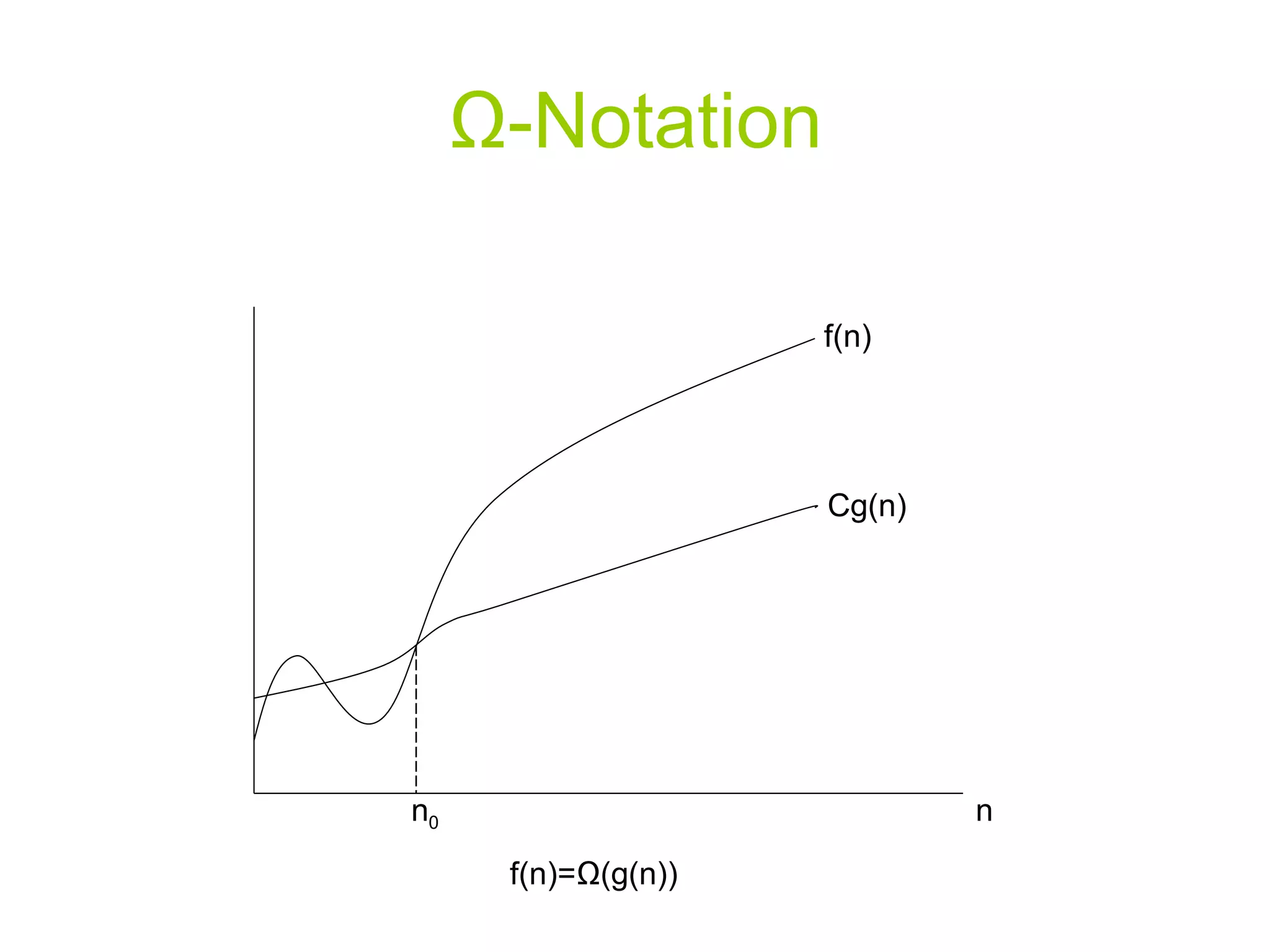

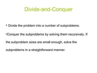
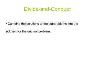
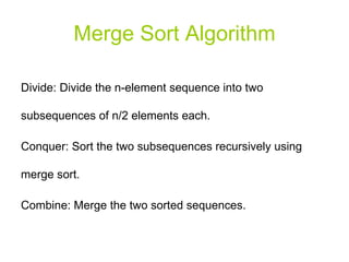
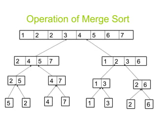
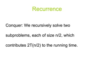
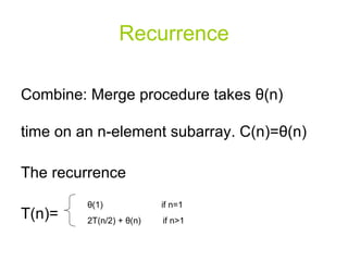
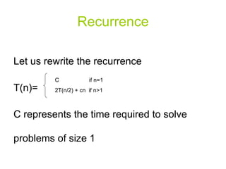
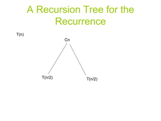
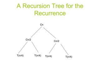
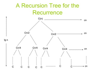
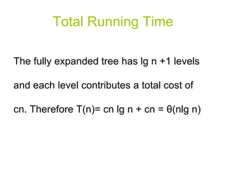
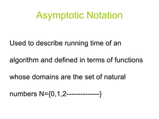
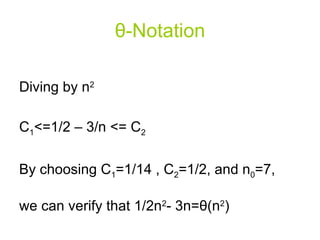
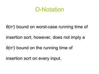
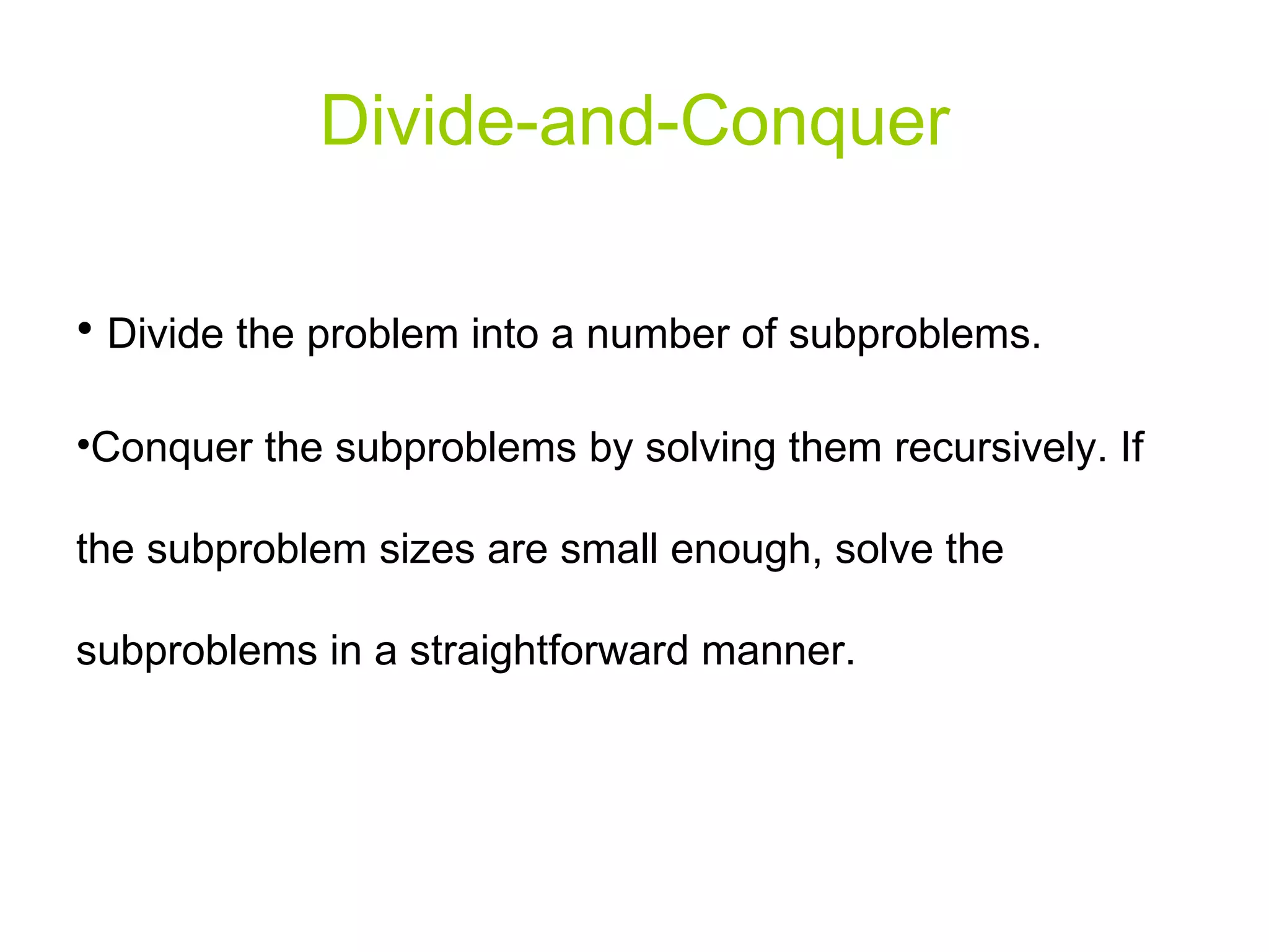
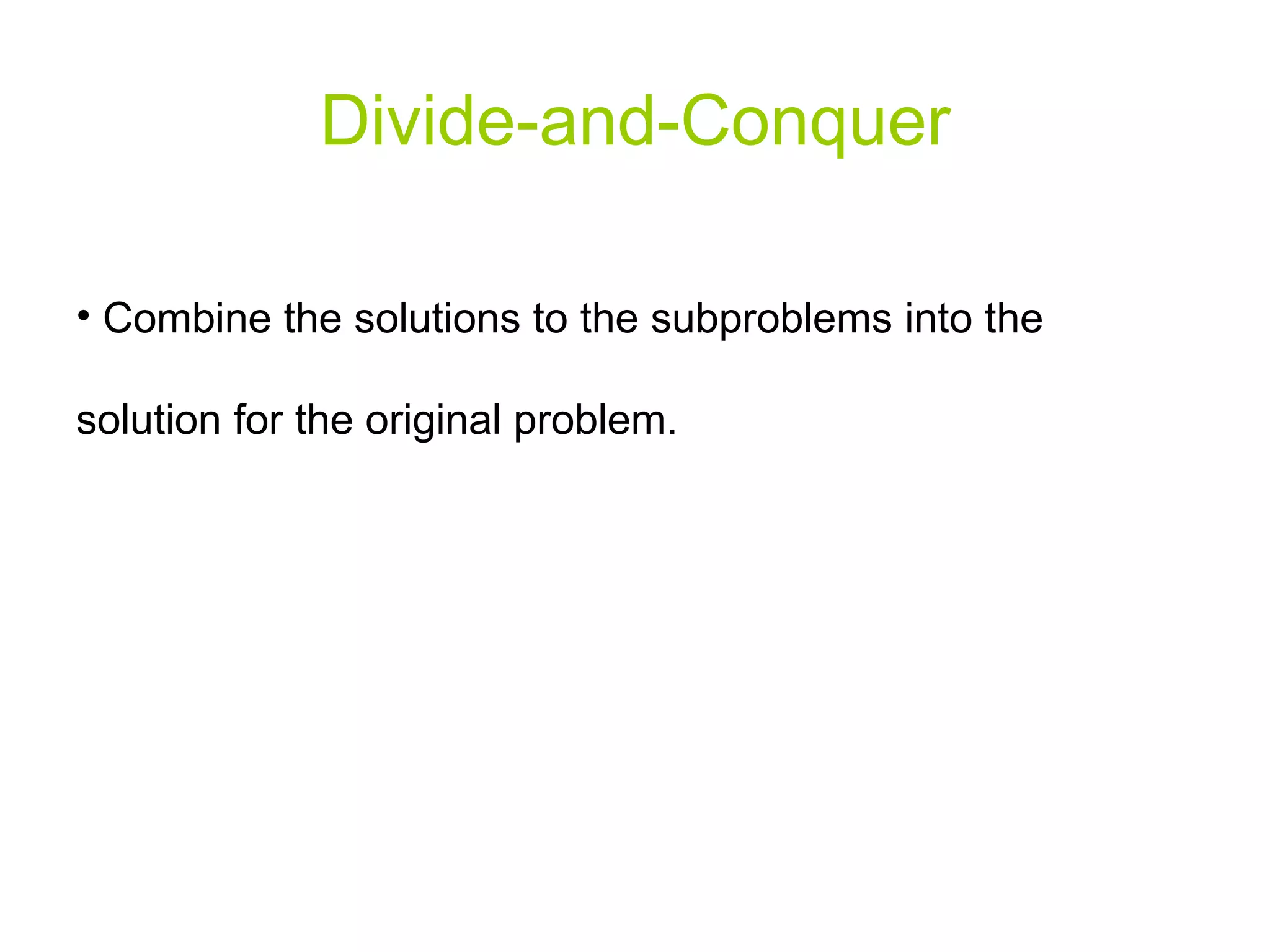
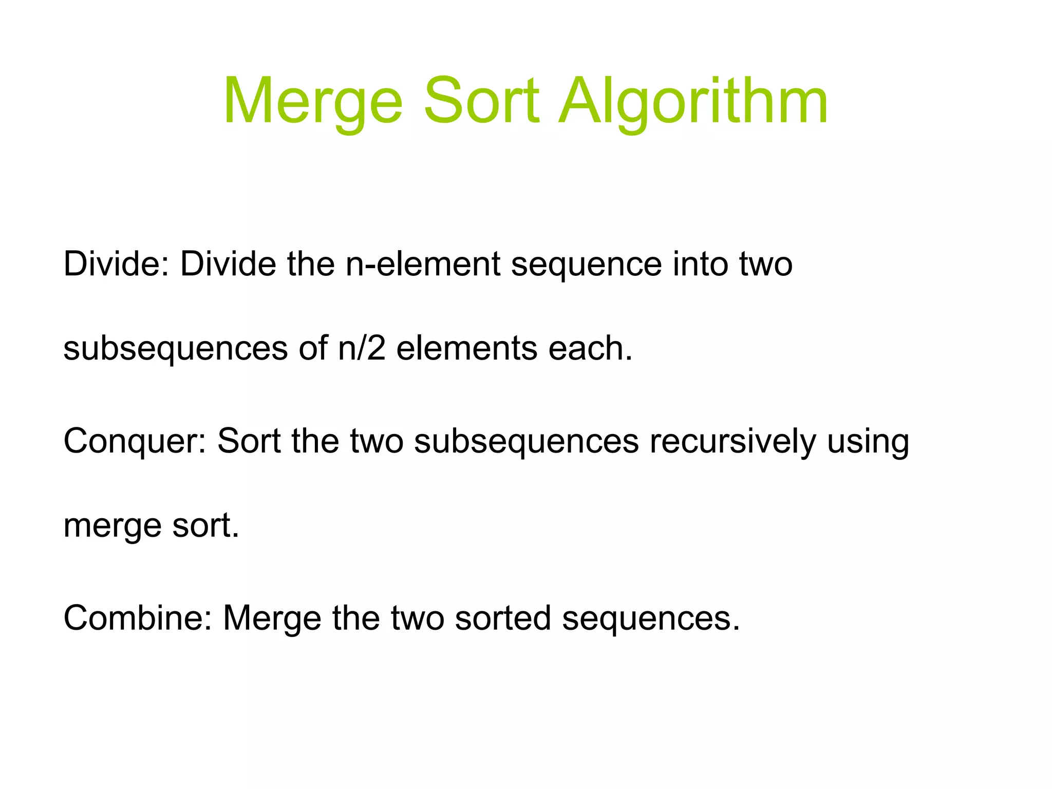
The document discusses divide and conquer algorithms and merge sort. It provides details on how merge sort works including: (1) Divide the input array into halves recursively until single element subarrays, (2) Sort the subarrays using merge sort recursively, (3) Merge the sorted subarrays back together. The overall running time of merge sort is analyzed to be θ(nlogn) as each level of recursion contributes θ(n) work and there are logn levels of recursion.


