
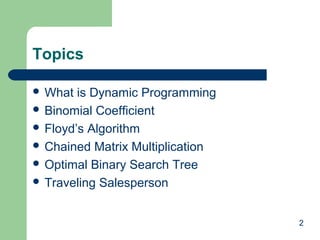

![Fib vs. fibDyn
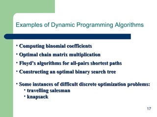
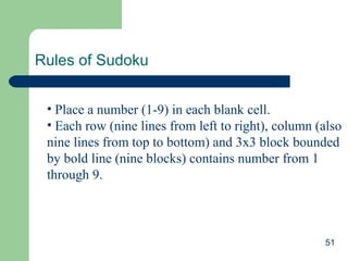
int fib(int n) {
if (n <= 1)
return n; // stopping conditions
else return fib(n-1) + fib(n-2);
// recursive step
}
int fibDyn(int n, vector<int>& fibList) {
int fibValue;
if (fibList[n] >= 0) // check for a previously computed result and return
return fibList[n];
// otherwise execute the recursive algorithm to obtain the result
if (n <= 1)
// stopping conditions
fibValue = n;
else
// recursive step
fibValue = fibDyn(n-1, fibList) + fibDyn(n-2, fibList);
// store the result and return its value
fibList[n] = fibValue;
return fibValue;
}
11](https://image.slidesharecdn.com/dynamicpgmming-131028044359-phpapp01/85/Dynamic-pgmming-11-320.jpg)

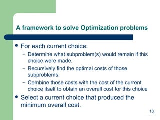
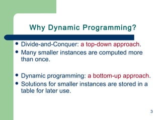
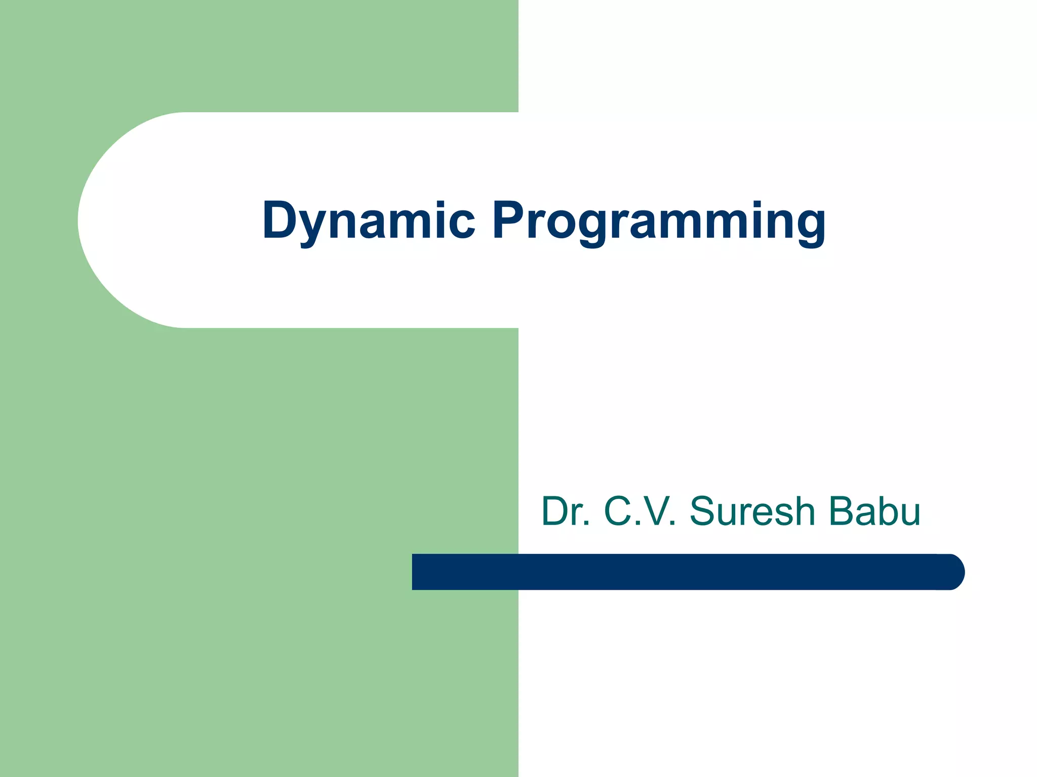
![Bottom-Up
Recursive
–
B[i] [j] =
property:
B[i – 1] [j – 1] + B[i – 1][j] 0 < j < i
1
j = 0 or j = i
25](https://image.slidesharecdn.com/dynamicpgmming-131028044359-phpapp01/85/Dynamic-pgmming-25-320.jpg)
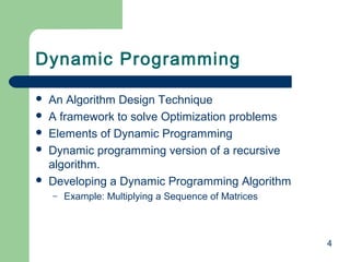
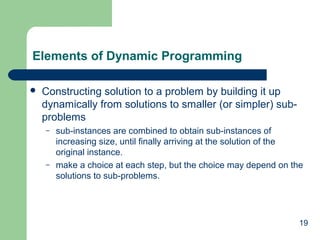
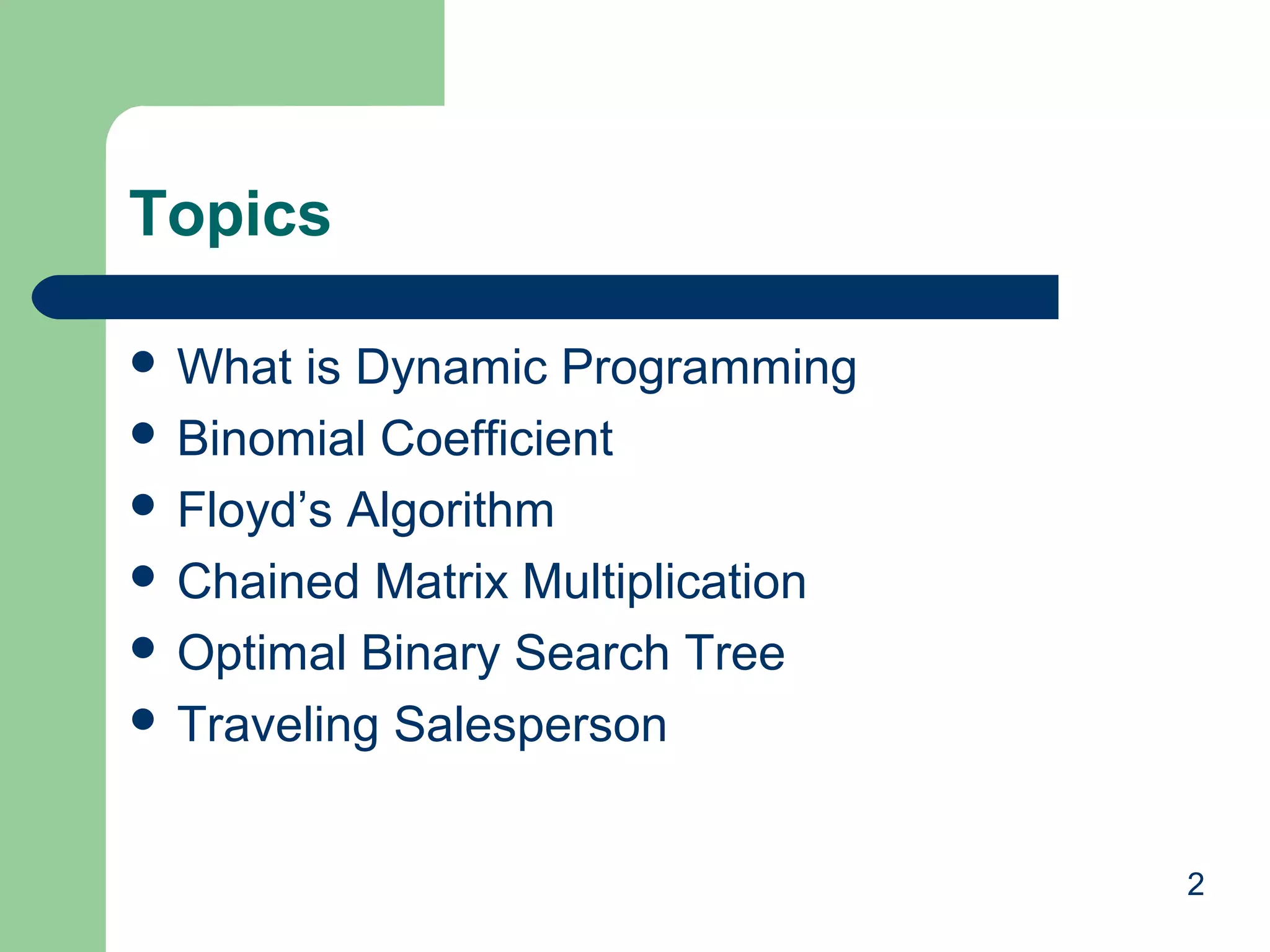
![Pascal’s Triangle
0
1
0
1
1
1
1
2
1
2
1
3
1
3
3 1
4
1
4
6 4
…
i
n
2
3 4
…
j
k
1
B[i-1][j-1]+ B[i-1][j]
B[i][j]
26](https://image.slidesharecdn.com/dynamicpgmming-131028044359-phpapp01/85/Dynamic-pgmming-26-320.jpg)
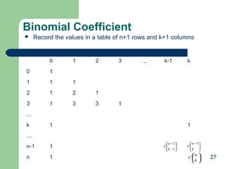
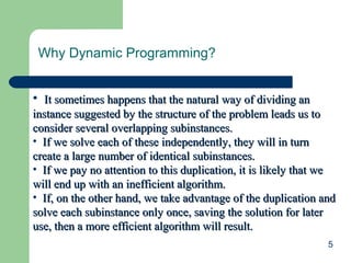
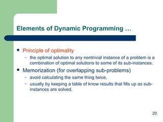
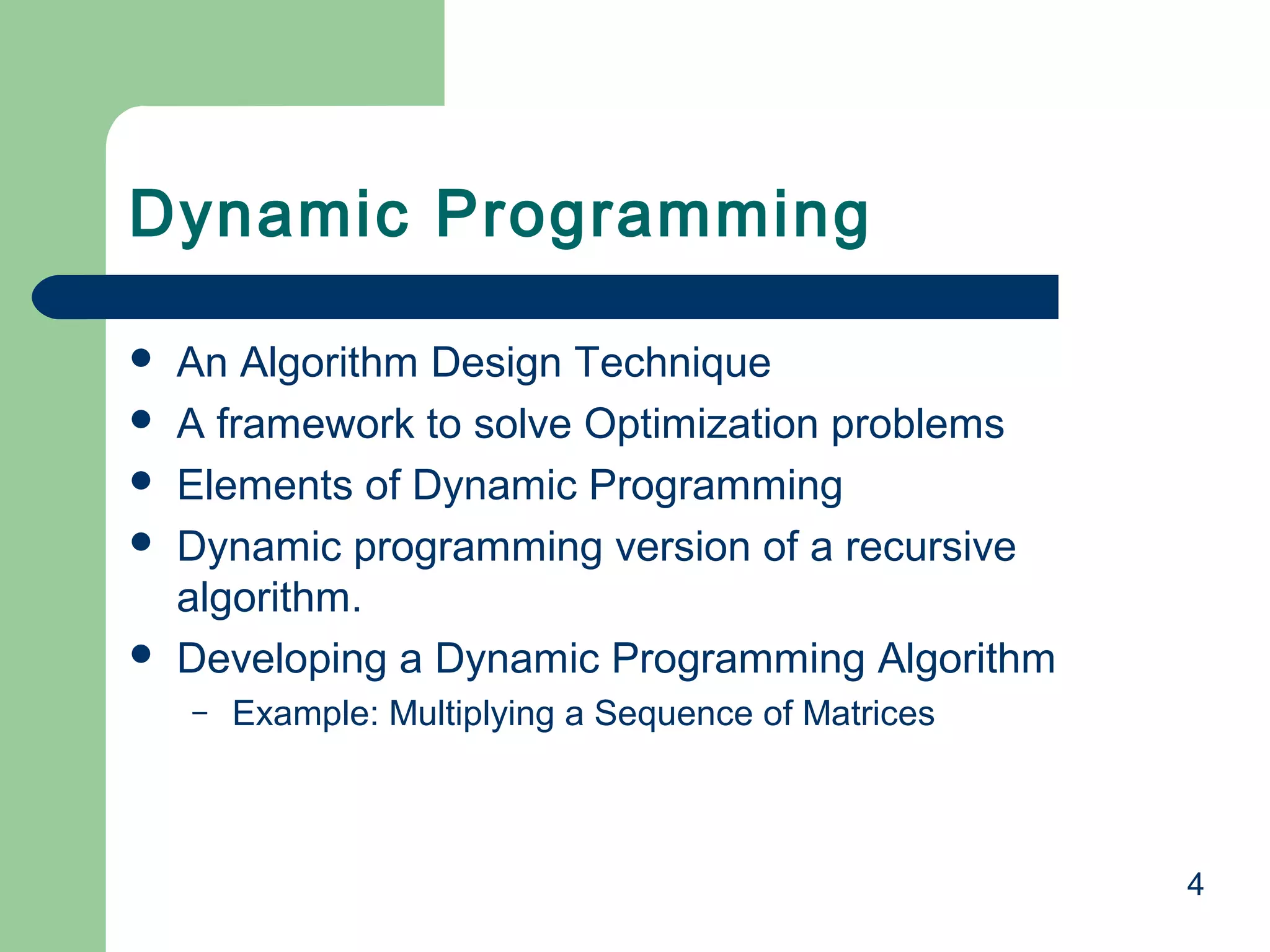
![Binomial Coefficient
ALGORITHM Binomial(n,k)
//Computes C(n, k) by the dynamic programming algorithm
//Input: A pair of nonnegative integers n ≥ k ≥ 0
//Output: The value of C(n ,k)
for i 0 to n do
for j 0 to min (i ,k) do
if j = 0 or j = k
C [i , j] 1
else C [i , j] C[i-1, j-1] + C[i-1, j]
return C [n, k]
k
i −1
A( n, k ) = ∑∑1 +
i =1 j =1
=
n
k
k
n
i =1
i =K +1
∑ ∑1 = ∑(i −1) + ∑k
i =k +1 j =1
( k −1) k
+ k ( n − k ) ∈Θ( nk )
2
28](https://image.slidesharecdn.com/dynamicpgmming-131028044359-phpapp01/85/Dynamic-pgmming-28-320.jpg)

![Meanings
D(0)[2][5] = lenth[v2, v5]= ∞
D(1)[2][5] = minimum(length[v2,v5], length[v2,v1,v5])
= minimum (∞, 14) = 14
D(2)[2][5] = D(1)[2][5] = 14
D(3)[2][5] = D(2)[2][5] = 14
D(4)[2][5] = minimum(length[v2,v1,v5], length[v2,v4,v5]),
length[v2,v1,v5], length[v2, v3,v4,v5]),
= minimum (14, 5, 13, 10) = 5
D(5)[2][5] = D(4)[2][5] = 5
32](https://image.slidesharecdn.com/dynamicpgmming-131028044359-phpapp01/85/Dynamic-pgmming-32-320.jpg)
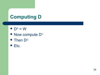
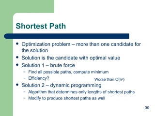
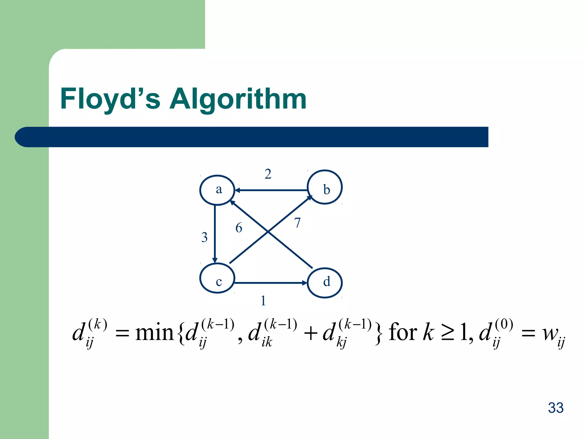
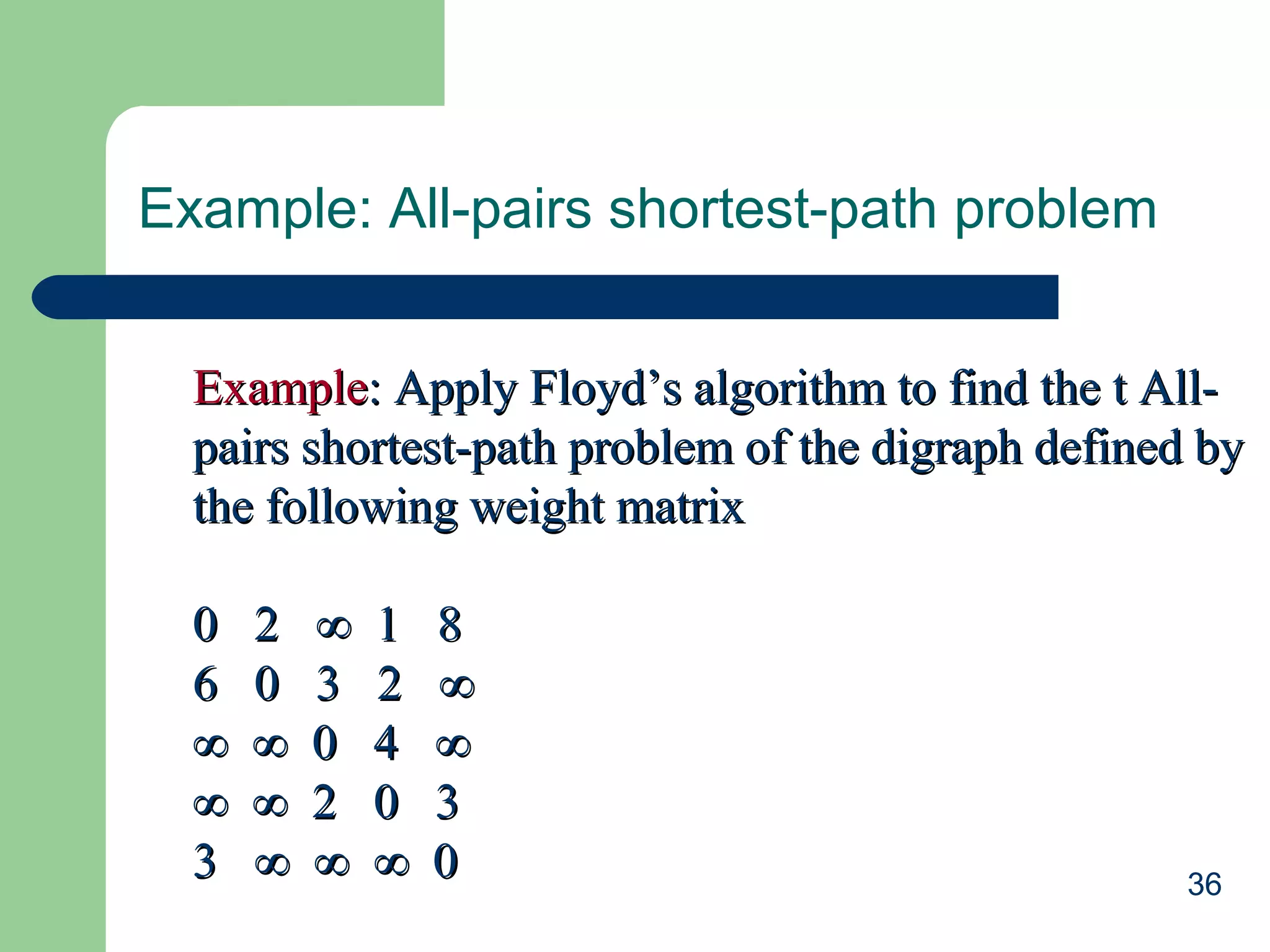
![Floyd’s Algorithm: All pairs shortest paths
• ALGORITHM Floyd (W[1 … n, 1… n])
•For k ← 1 to n do
•For i ← 1 to n do
•For j ← 1 to n do
•W[i, j] ← min{W[i,j], W{i, k] + W[k, j]}
•Return W
•Efficiency = ?
Θ(n)
35](https://image.slidesharecdn.com/dynamicpgmming-131028044359-phpapp01/85/Dynamic-pgmming-35-320.jpg)


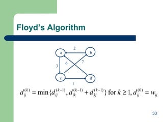
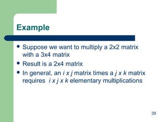
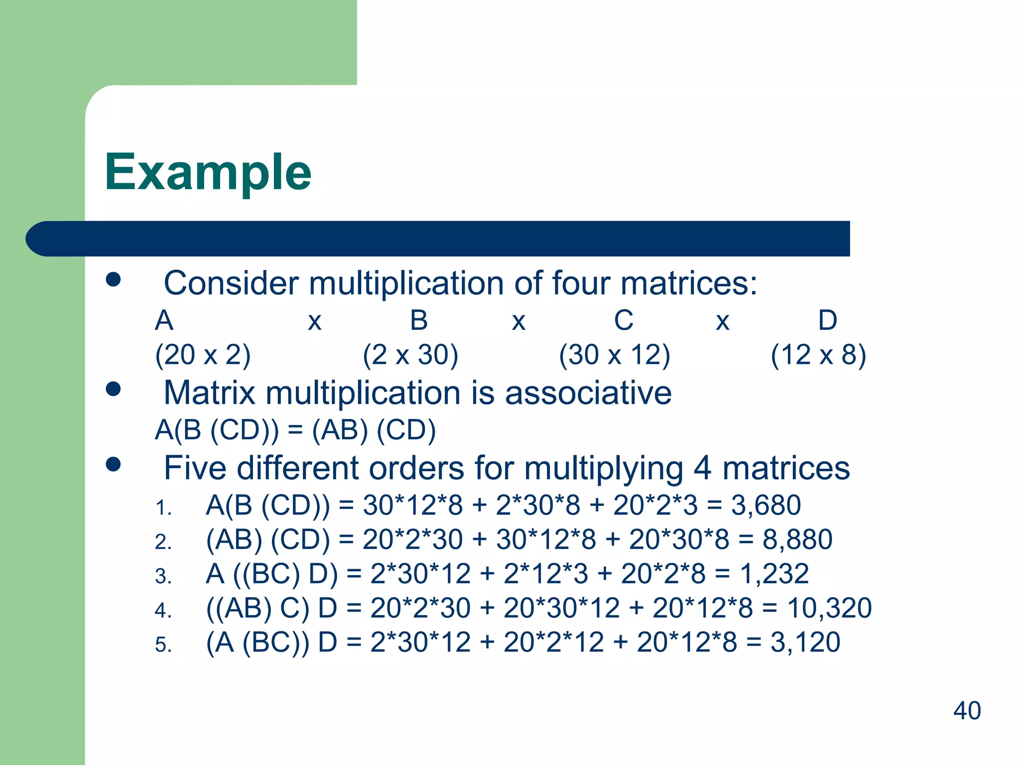
![Chained Matrix Multiplication
Problem: Matrix-chain multiplication
– a chain of <A1, A2, …, An> of n matrices
–
find a way that minimizes the number of scalar multiplications to
compute the product A1A2…An
Strategy:
Breaking a problem into sub-problem
– A1A2...Ak, Ak+1Ak+2…An
Recursively define the value of an optimal solution
– m[i,j] = 0 if i = j
– m[i,j]= min{i<=k<j} (m[i,k]+m[k+1,j]+pi-1pkpj)
–
for 1 <= i <= j <= n
38](https://image.slidesharecdn.com/dynamicpgmming-131028044359-phpapp01/85/Dynamic-pgmming-38-320.jpg)
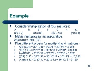
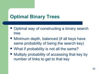
![Algorithm
int minmult (int n, const ind d[], index P[ ] [ ])
{
index i, j, k, diagonal;
int M[1..n][1..n];
for (i = 1; i <= n; i++)
M[i][i] = 0;
for (diagonal = 1; diagonal <= n-1; diagonal++)
for (i = 1; i <= n-diagonal; i++)
{
j = i + diagonal;
M[i] [j] = minimum(M[i][k] + M[k+1][j] + d[i-1]*d[k]*d[j]);
// minimun (i <= k <= j-1)
P[i] [j] = a value of k that gave the minimum;
}
return M[1][n];
}
41](https://image.slidesharecdn.com/dynamicpgmming-131028044359-phpapp01/85/Dynamic-pgmming-41-320.jpg)


![Fib vs. fibDyn
int fib(int n) {
if (n <= 1)
return n; // stopping conditions
else return fib(n-1) + fib(n-2);
// recursive step
}
int fibDyn(int n, vector<int>& fibList) {
int fibValue;
if (fibList[n] >= 0) // check for a previously computed result and return
return fibList[n];
// otherwise execute the recursive algorithm to obtain the result
if (n <= 1)
// stopping conditions
fibValue = n;
else
// recursive step
fibValue = fibDyn(n-1, fibList) + fibDyn(n-2, fibList);
// store the result and return its value
fibList[n] = fibValue;
return fibValue;
}
11](https://image.slidesharecdn.com/dynamicpgmming-131028044359-phpapp01/75/Dynamic-pgmming-11-2048.jpg)


![Bottom-Up
Recursive
–
B[i] [j] =
property:
B[i – 1] [j – 1] + B[i – 1][j] 0 < j < i
1
j = 0 or j = i
25](https://image.slidesharecdn.com/dynamicpgmming-131028044359-phpapp01/75/Dynamic-pgmming-25-2048.jpg)
![Pascal’s Triangle
0
1
0
1
1
1
1
2
1
2
1
3
1
3
3 1
4
1
4
6 4
…
i
n
2
3 4
…
j
k
1
B[i-1][j-1]+ B[i-1][j]
B[i][j]
26](https://image.slidesharecdn.com/dynamicpgmming-131028044359-phpapp01/75/Dynamic-pgmming-26-2048.jpg)
![Binomial Coefficient
ALGORITHM Binomial(n,k)
//Computes C(n, k) by the dynamic programming algorithm
//Input: A pair of nonnegative integers n ≥ k ≥ 0
//Output: The value of C(n ,k)
for i 0 to n do
for j 0 to min (i ,k) do
if j = 0 or j = k
C [i , j] 1
else C [i , j] C[i-1, j-1] + C[i-1, j]
return C [n, k]
k
i −1
A( n, k ) = ∑∑1 +
i =1 j =1
=
n
k
k
n
i =1
i =K +1
∑ ∑1 = ∑(i −1) + ∑k
i =k +1 j =1
( k −1) k
+ k ( n − k ) ∈Θ( nk )
2
28](https://image.slidesharecdn.com/dynamicpgmming-131028044359-phpapp01/75/Dynamic-pgmming-28-2048.jpg)

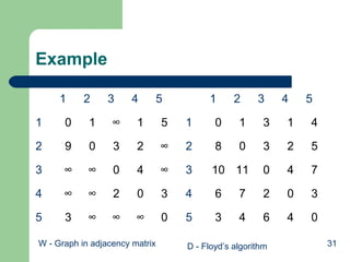
![Meanings
D(0)[2][5] = lenth[v2, v5]= ∞
D(1)[2][5] = minimum(length[v2,v5], length[v2,v1,v5])
= minimum (∞, 14) = 14
D(2)[2][5] = D(1)[2][5] = 14
D(3)[2][5] = D(2)[2][5] = 14
D(4)[2][5] = minimum(length[v2,v1,v5], length[v2,v4,v5]),
length[v2,v1,v5], length[v2, v3,v4,v5]),
= minimum (14, 5, 13, 10) = 5
D(5)[2][5] = D(4)[2][5] = 5
32](https://image.slidesharecdn.com/dynamicpgmming-131028044359-phpapp01/75/Dynamic-pgmming-32-2048.jpg)

![Floyd’s Algorithm: All pairs shortest paths
• ALGORITHM Floyd (W[1 … n, 1… n])
•For k ← 1 to n do
•For i ← 1 to n do
•For j ← 1 to n do
•W[i, j] ← min{W[i,j], W{i, k] + W[k, j]}
•Return W
•Efficiency = ?
Θ(n)
35](https://image.slidesharecdn.com/dynamicpgmming-131028044359-phpapp01/75/Dynamic-pgmming-35-2048.jpg)

![Chained Matrix Multiplication
Problem: Matrix-chain multiplication
– a chain of <A1, A2, …, An> of n matrices
–
find a way that minimizes the number of scalar multiplications to
compute the product A1A2…An
Strategy:
Breaking a problem into sub-problem
– A1A2...Ak, Ak+1Ak+2…An
Recursively define the value of an optimal solution
– m[i,j] = 0 if i = j
– m[i,j]= min{i<=k<j} (m[i,k]+m[k+1,j]+pi-1pkpj)
–
for 1 <= i <= j <= n
38](https://image.slidesharecdn.com/dynamicpgmming-131028044359-phpapp01/75/Dynamic-pgmming-38-2048.jpg)

![Algorithm
int minmult (int n, const ind d[], index P[ ] [ ])
{
index i, j, k, diagonal;
int M[1..n][1..n];
for (i = 1; i <= n; i++)
M[i][i] = 0;
for (diagonal = 1; diagonal <= n-1; diagonal++)
for (i = 1; i <= n-diagonal; i++)
{
j = i + diagonal;
M[i] [j] = minimum(M[i][k] + M[k+1][j] + d[i-1]*d[k]*d[j]);
// minimun (i <= k <= j-1)
P[i] [j] = a value of k that gave the minimum;
}
return M[1][n];
}
41](https://image.slidesharecdn.com/dynamicpgmming-131028044359-phpapp01/75/Dynamic-pgmming-41-2048.jpg)


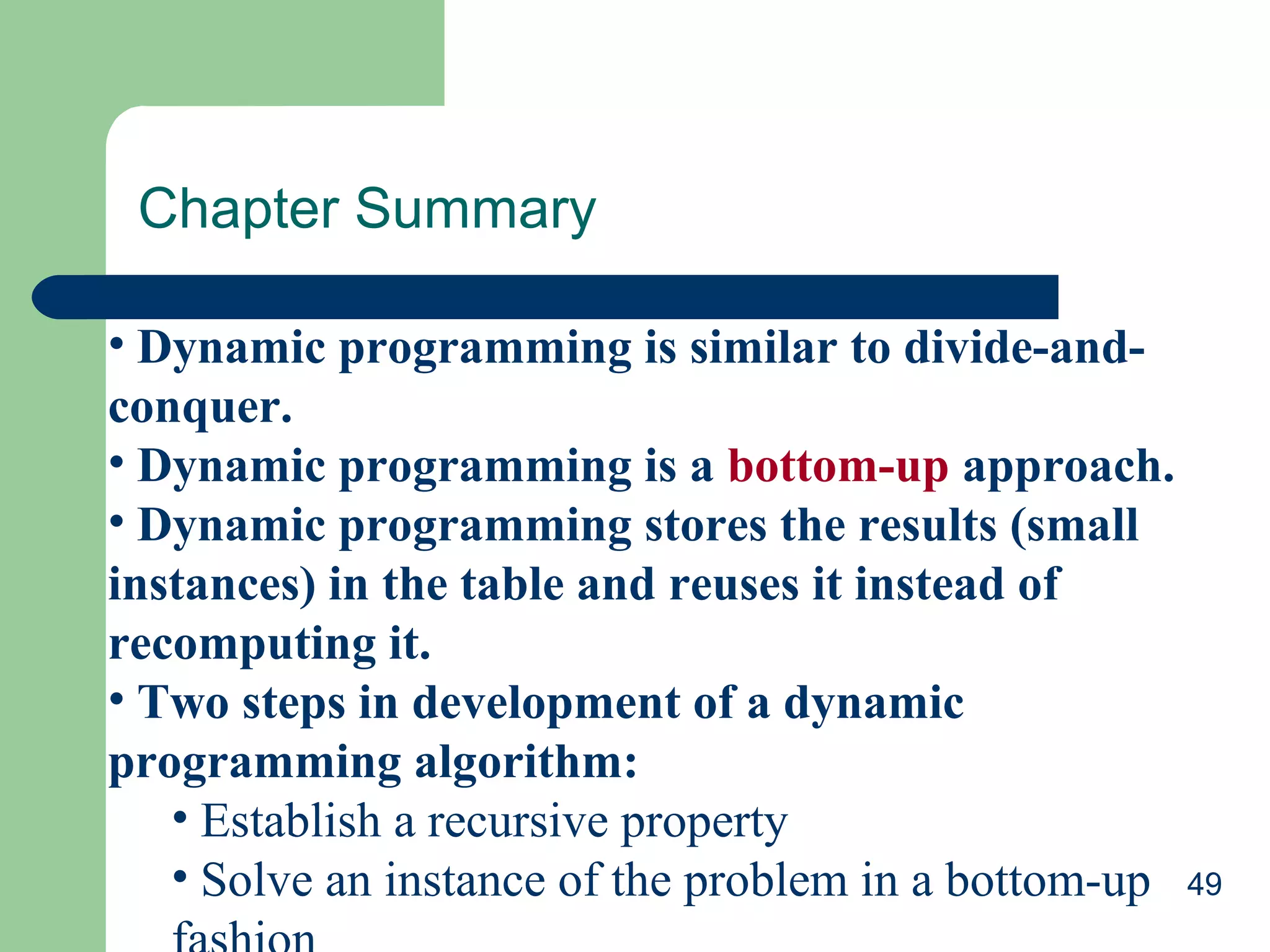

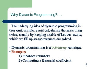
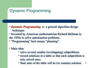
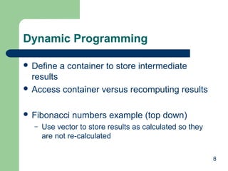
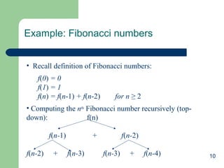
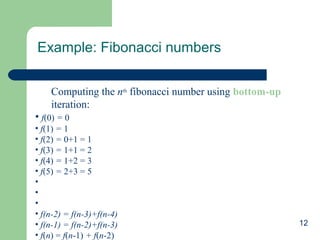
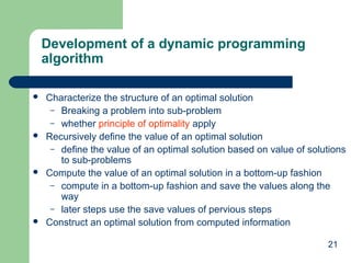
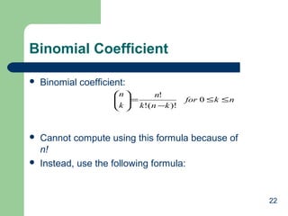
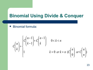
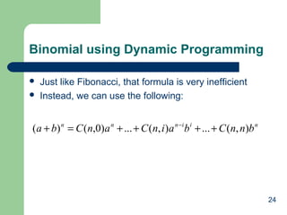
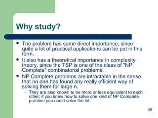
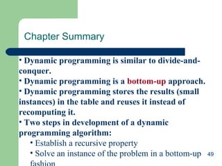
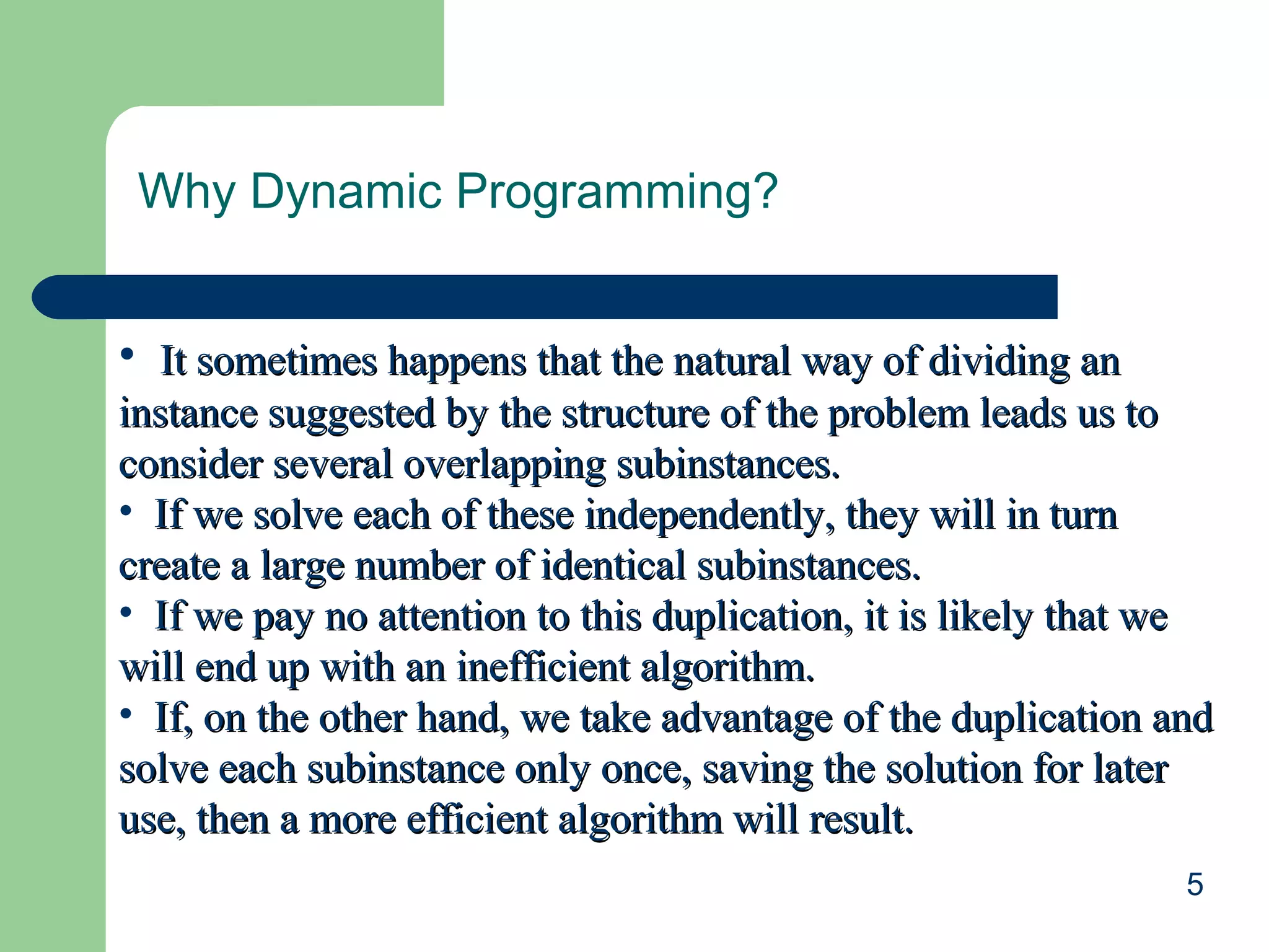
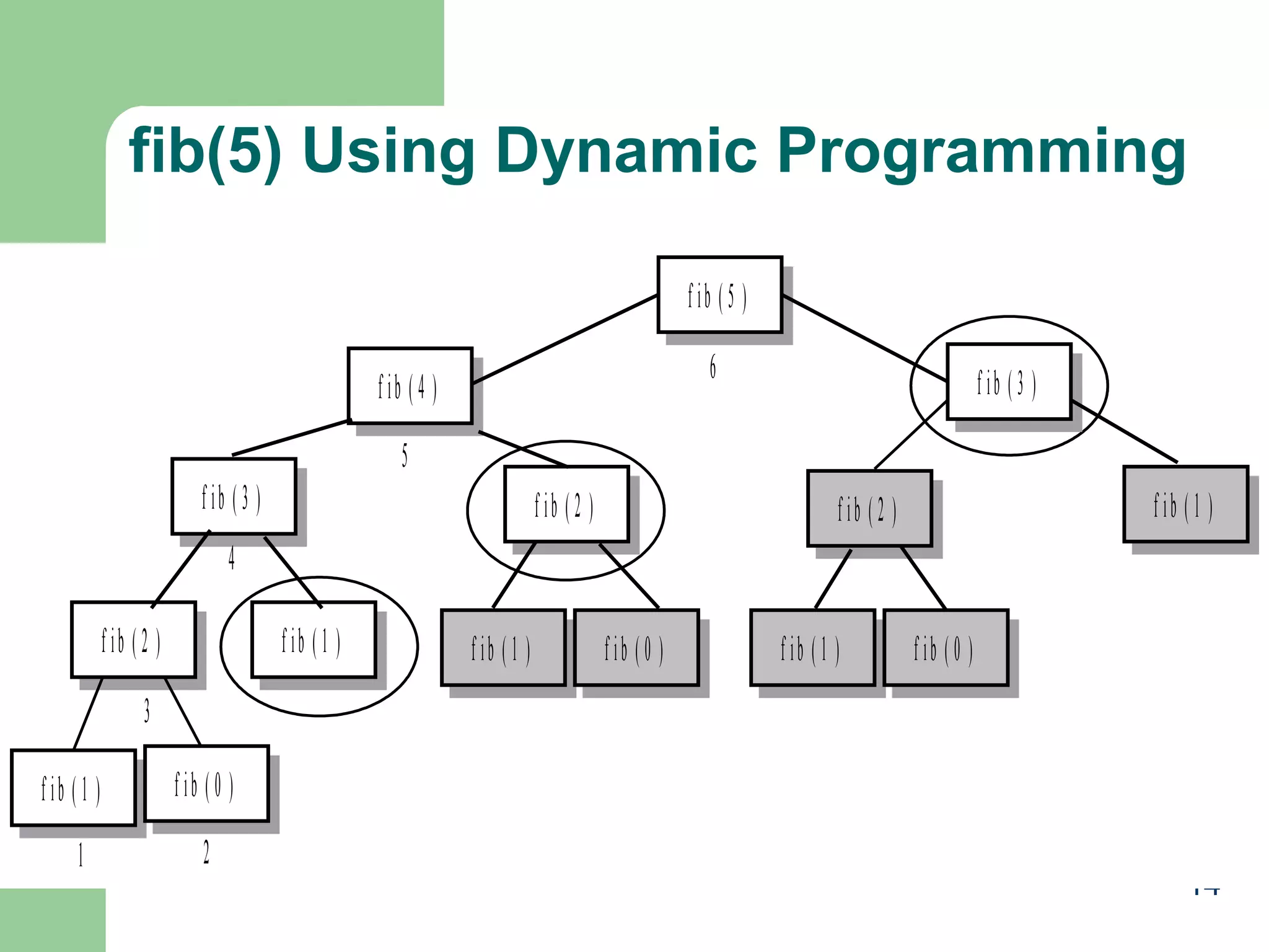
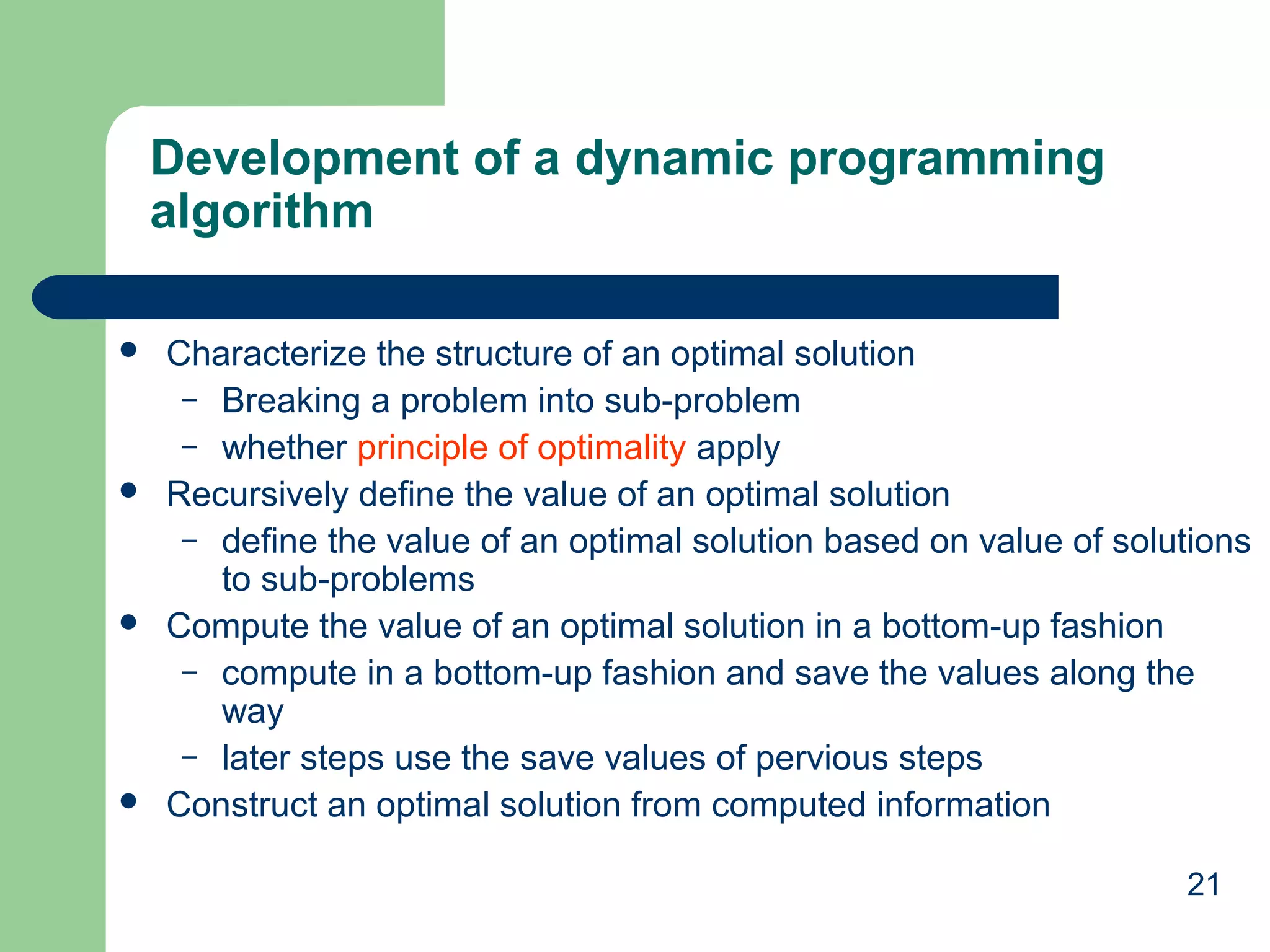
This document provides an overview of dynamic programming. It begins by explaining that dynamic programming is a technique for solving optimization problems by breaking them down into overlapping subproblems and storing the results of solved subproblems in a table to avoid recomputing them. It then provides examples of problems that can be solved using dynamic programming, including Fibonacci numbers, binomial coefficients, shortest paths, and optimal binary search trees. The key aspects of dynamic programming algorithms, including defining subproblems and combining their solutions, are also outlined.


