Introduction to dynamic programming

Introduction to dynamic programming

• 1.
  TOPIC: Introduction to dynamicprogramming and problem solving BY: PREYASH MISTRY(160110107029) NARSINGANI AMISHA(160110107031) G H Patel College Of Engineering & Technology, V.V.Nagar
• 2.
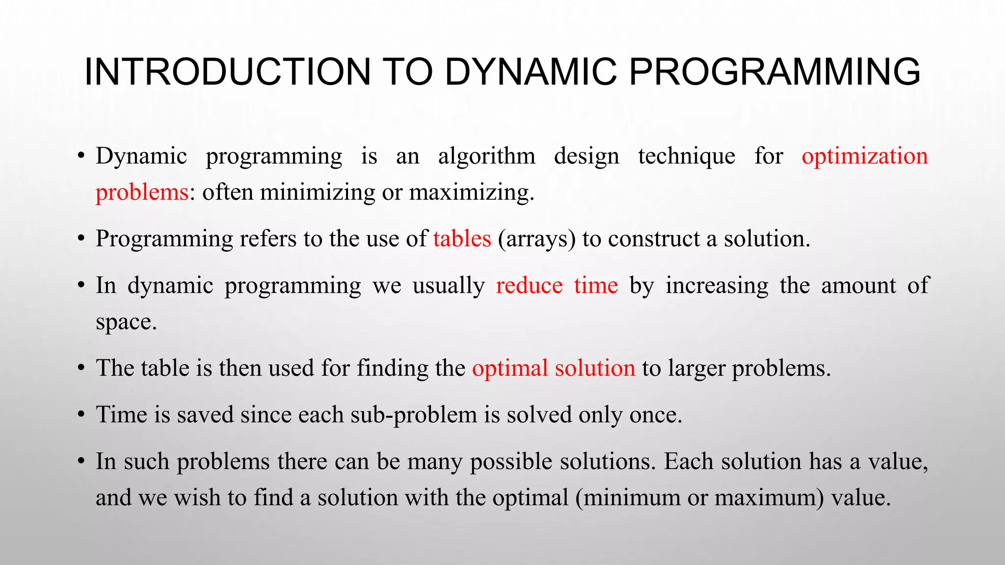
  INTRODUCTION TO DYNAMICPROGRAMMING • Dynamic programming is an algorithm design technique for optimization problems: often minimizing or maximizing. • Programming refers to the use of tables (arrays) to construct a solution. • In dynamic programming we usually reduce time by increasing the amount of space. • The table is then used for finding the optimal solution to larger problems. • Time is saved since each sub-problem is solved only once. • In such problems there can be many possible solutions. Each solution has a value, and we wish to find a solution with the optimal (minimum or maximum) value.
• 3.
  STEPS FOR THEDEVELOPMENT OF DYNAMIC PROGRAMMING 1. Characterize the structure of an optimal solution 2. Recursively define the value of an optimal solution 3. Compute the value of an optimal solution in a bottom-up fashion 4. Construct an optimal solution from computed information (not always necessary)
• 4.
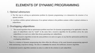
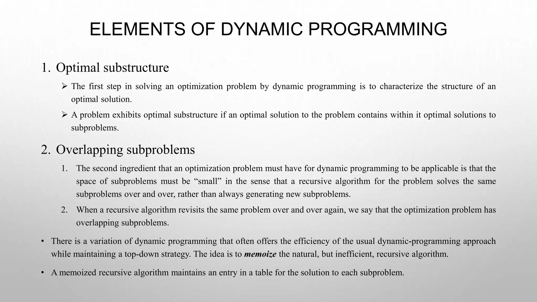
  ELEMENTS OF DYNAMICPROGRAMMING 1. Optimal substructure  The first step in solving an optimization problem by dynamic programming is to characterize the structure of an optimal solution.  A problem exhibits optimal substructure if an optimal solution to the problem contains within it optimal solutions to subproblems. 2. Overlapping subproblems 1. The second ingredient that an optimization problem must have for dynamic programming to be applicable is that the space of subproblems must be “small” in the sense that a recursive algorithm for the problem solves the same subproblems over and over, rather than always generating new subproblems. 2. When a recursive algorithm revisits the same problem over and over again, we say that the optimization problem has overlapping subproblems. • There is a variation of dynamic programming that often offers the efficiency of the usual dynamic-programming approach while maintaining a top-down strategy. The idea is to memoize the natural, but inefficient, recursive algorithm. • A memoized recursive algorithm maintains an entry in a table for the solution to each subproblem.
• 5.
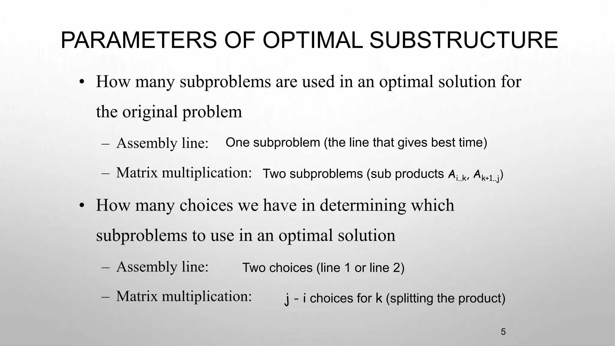
  5 PARAMETERS OF OPTIMALSUBSTRUCTURE • How many subproblems are used in an optimal solution for the original problem – Assembly line: – Matrix multiplication: • How many choices we have in determining which subproblems to use in an optimal solution – Assembly line: – Matrix multiplication: One subproblem (the line that gives best time) Two choices (line 1 or line 2) Two subproblems (sub products Ai..k, Ak+1..j) j - i choices for k (splitting the product)
• 6.
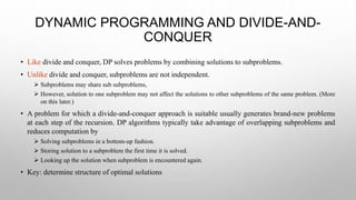
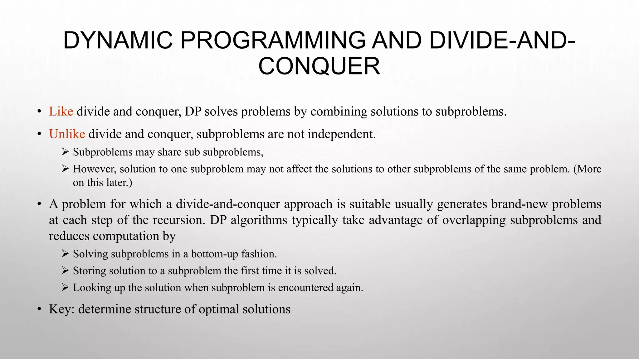
  DYNAMIC PROGRAMMING ANDDIVIDE-AND- CONQUER • Like divide and conquer, DP solves problems by combining solutions to subproblems. • Unlike divide and conquer, subproblems are not independent.  Subproblems may share sub subproblems,  However, solution to one subproblem may not affect the solutions to other subproblems of the same problem. (More on this later.) • A problem for which a divide-and-conquer approach is suitable usually generates brand-new problems at each step of the recursion. DP algorithms typically take advantage of overlapping subproblems and reduces computation by  Solving subproblems in a bottom-up fashion.  Storing solution to a subproblem the first time it is solved.  Looking up the solution when subproblem is encountered again. • Key: determine structure of optimal solutions
• 7.
  PROBLEMS REPRESENTING DYNAMIC PROGRAMMING •The best way to get a feel for this is through some more examples.  Matrix chaining optimization  Longest common subsequence  0-1 knapsack problem  Transitive closure of a direct graph  All point shortest path  Binomial co-efficient
• 8.
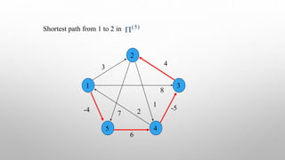
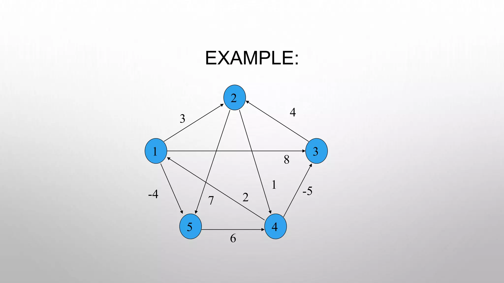
  PRINCIPLE OF OPTIMALITY •Obtains the solution using principle of optimality. • In an optimal sequence of decisions or choices, each subsequence must also be optimal. • When it is not possible to apply the principle of optimality it is almost impossible to obtain the solution using the dynamic programming approach. • Example: finding of shortest path in a given graph uses the principle of optimality.
• 9.
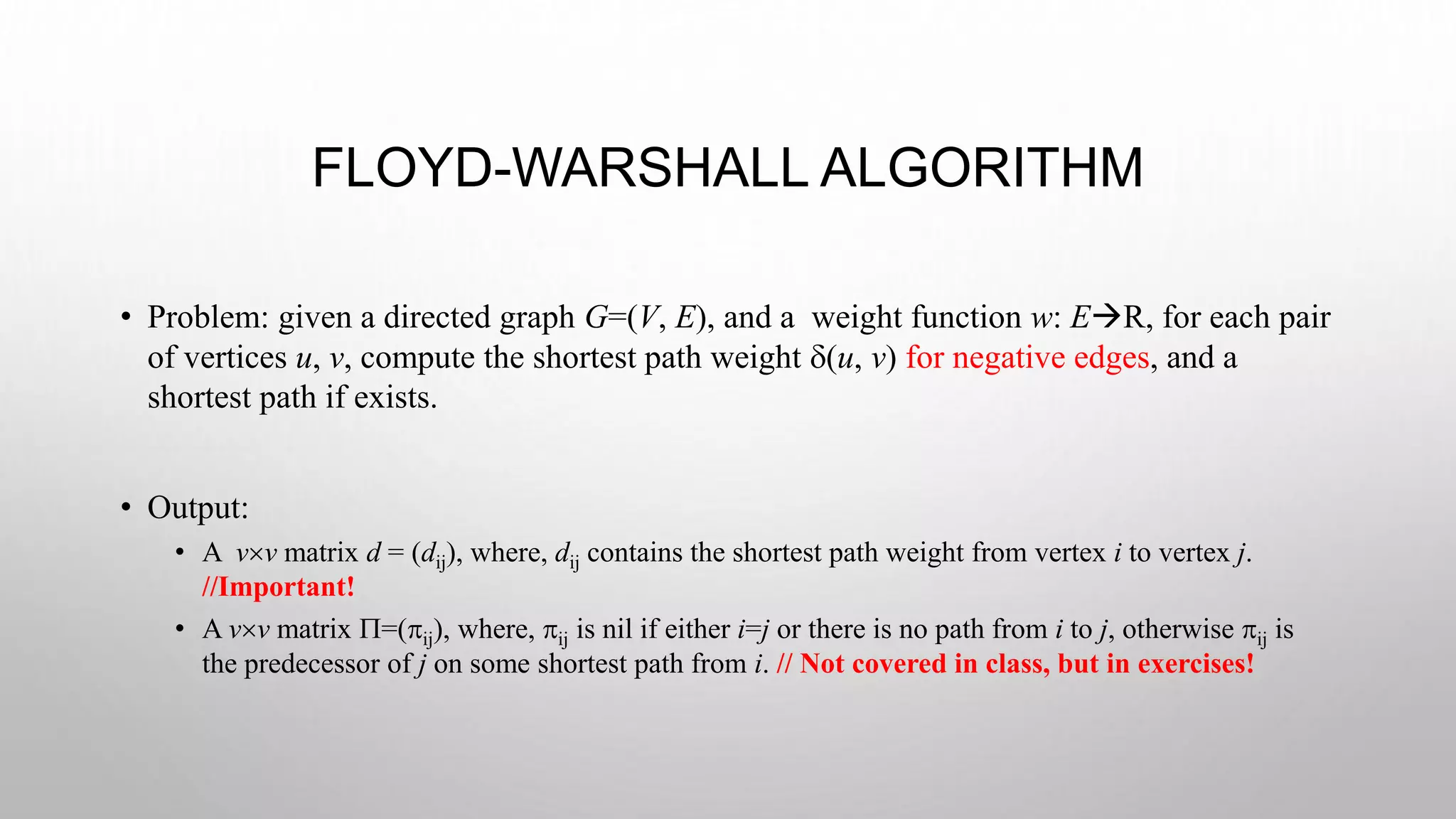
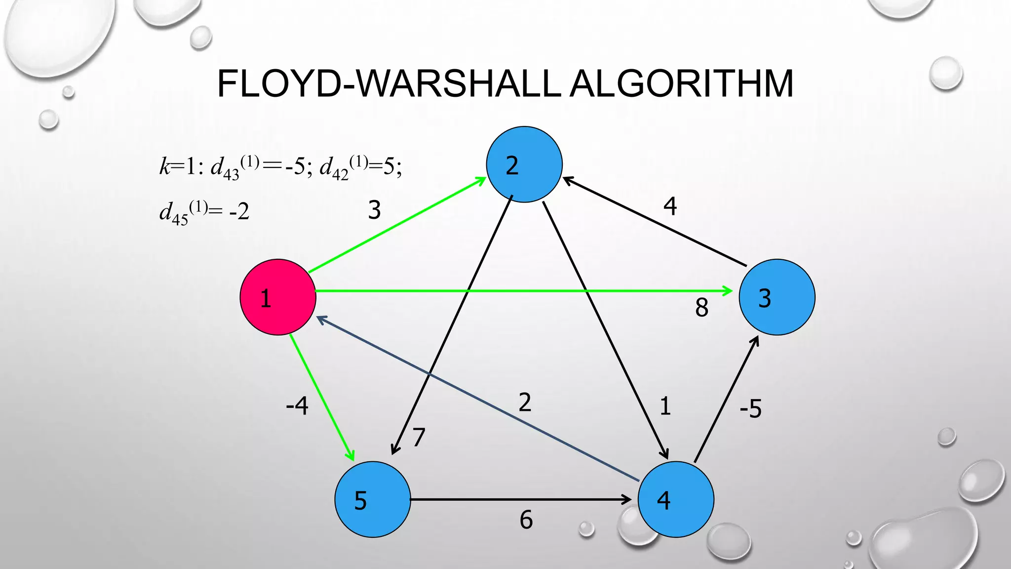
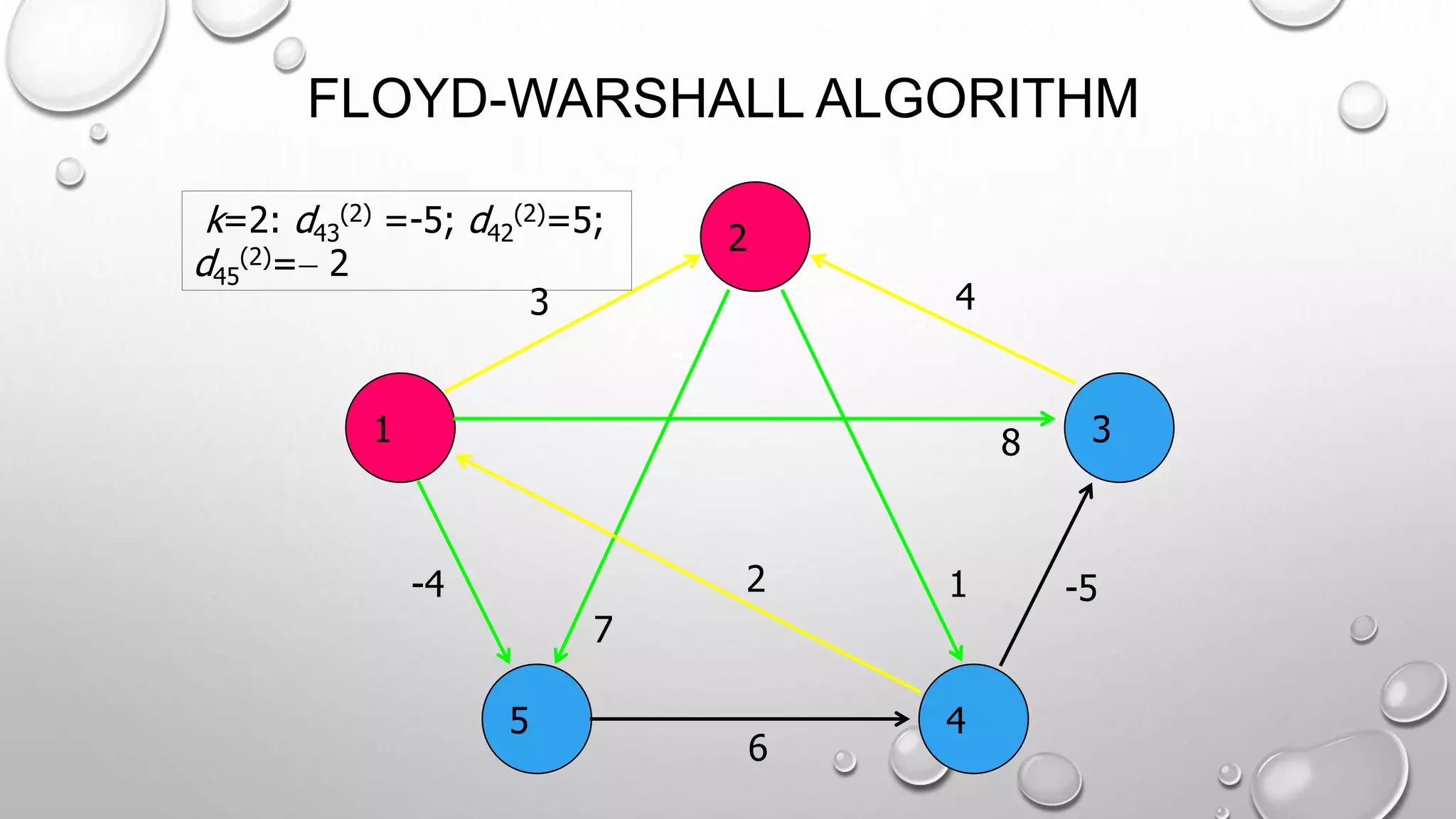
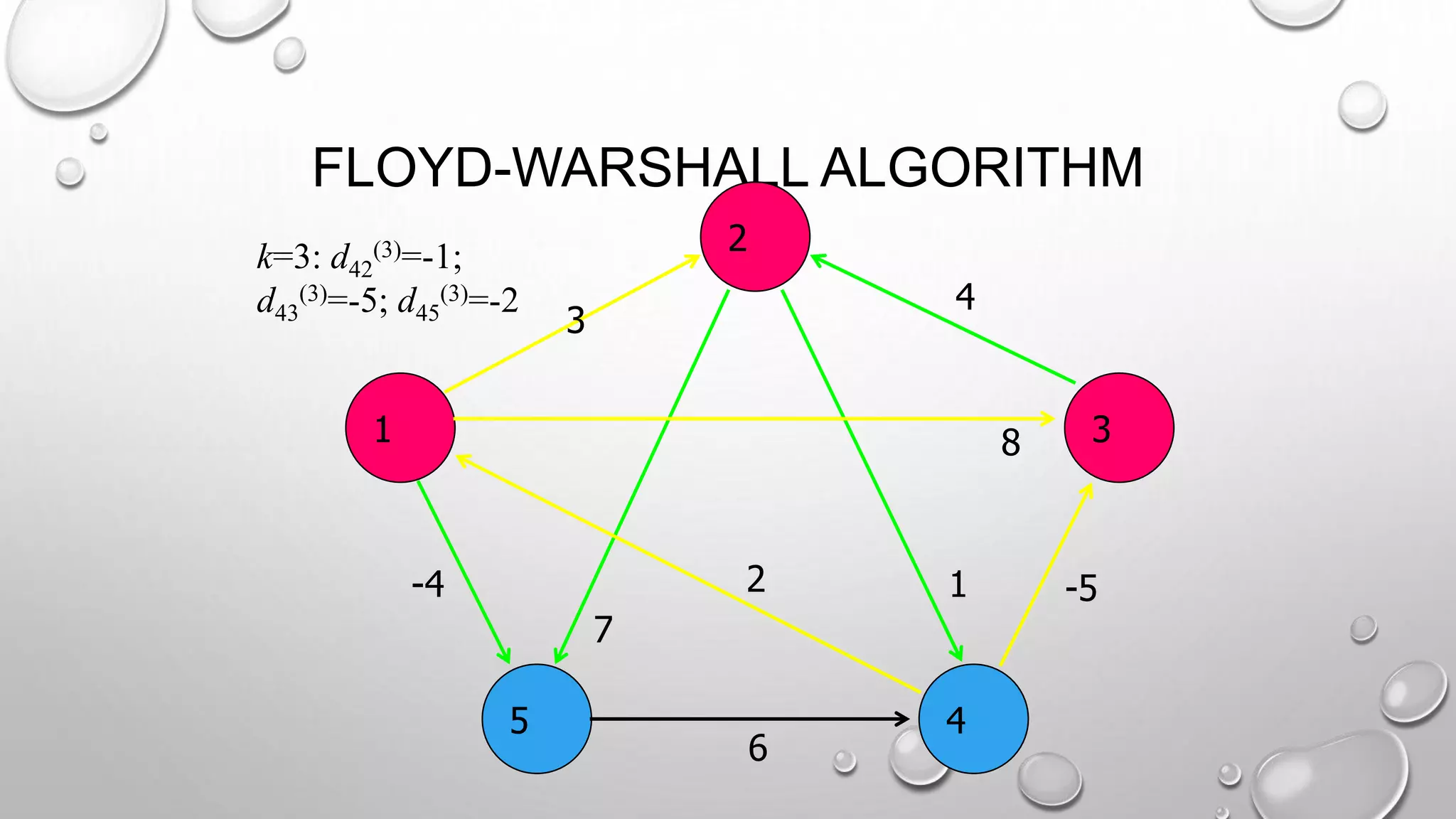
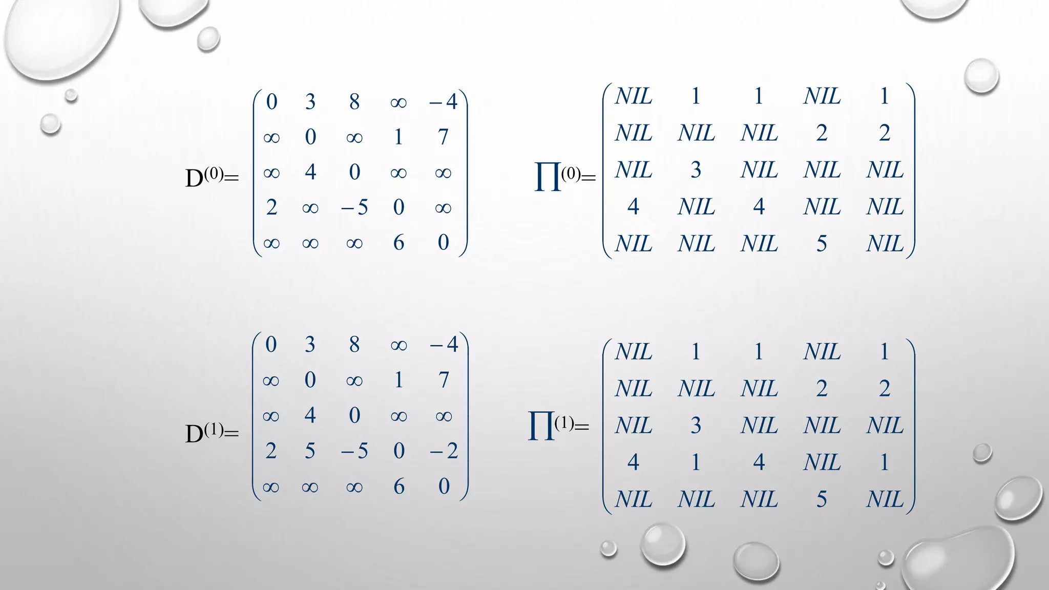
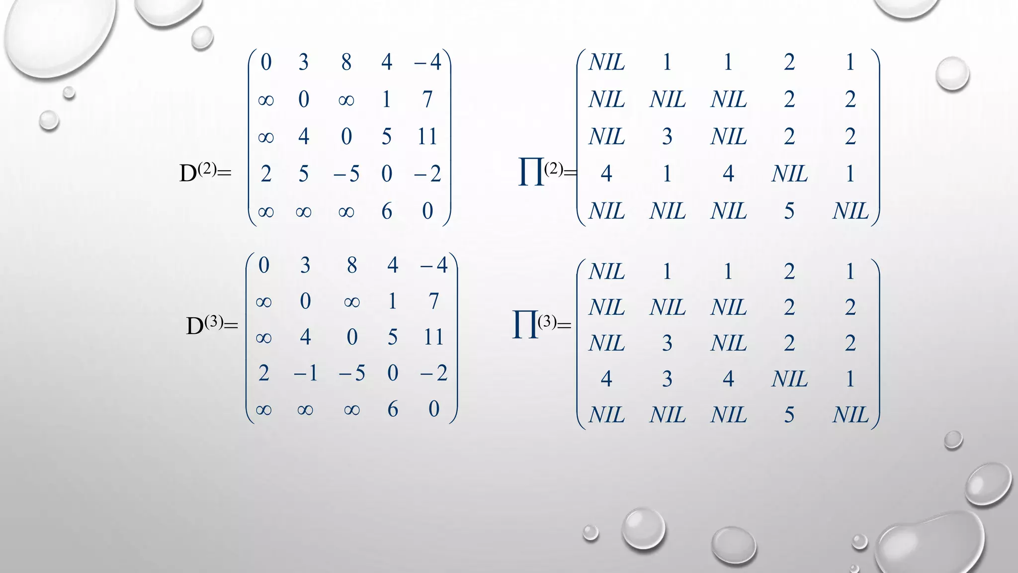
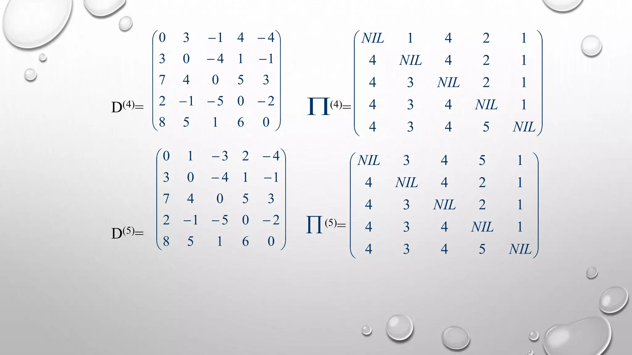
  FLOYD-WARSHALL ALGORITHM • Problem:given a directed graph G=(V, E), and a weight function w: ER, for each pair of vertices u, v, compute the shortest path weight (u, v) for negative edges, and a shortest path if exists. • Output: • A vv matrix d = (dij), where, dij contains the shortest path weight from vertex i to vertex j. //Important! • A vv matrix =(ij), where, ij is nil if either i=j or there is no path from i to j, otherwise ij is the predecessor of j on some shortest path from i. // Not covered in class, but in exercises!
• 10.
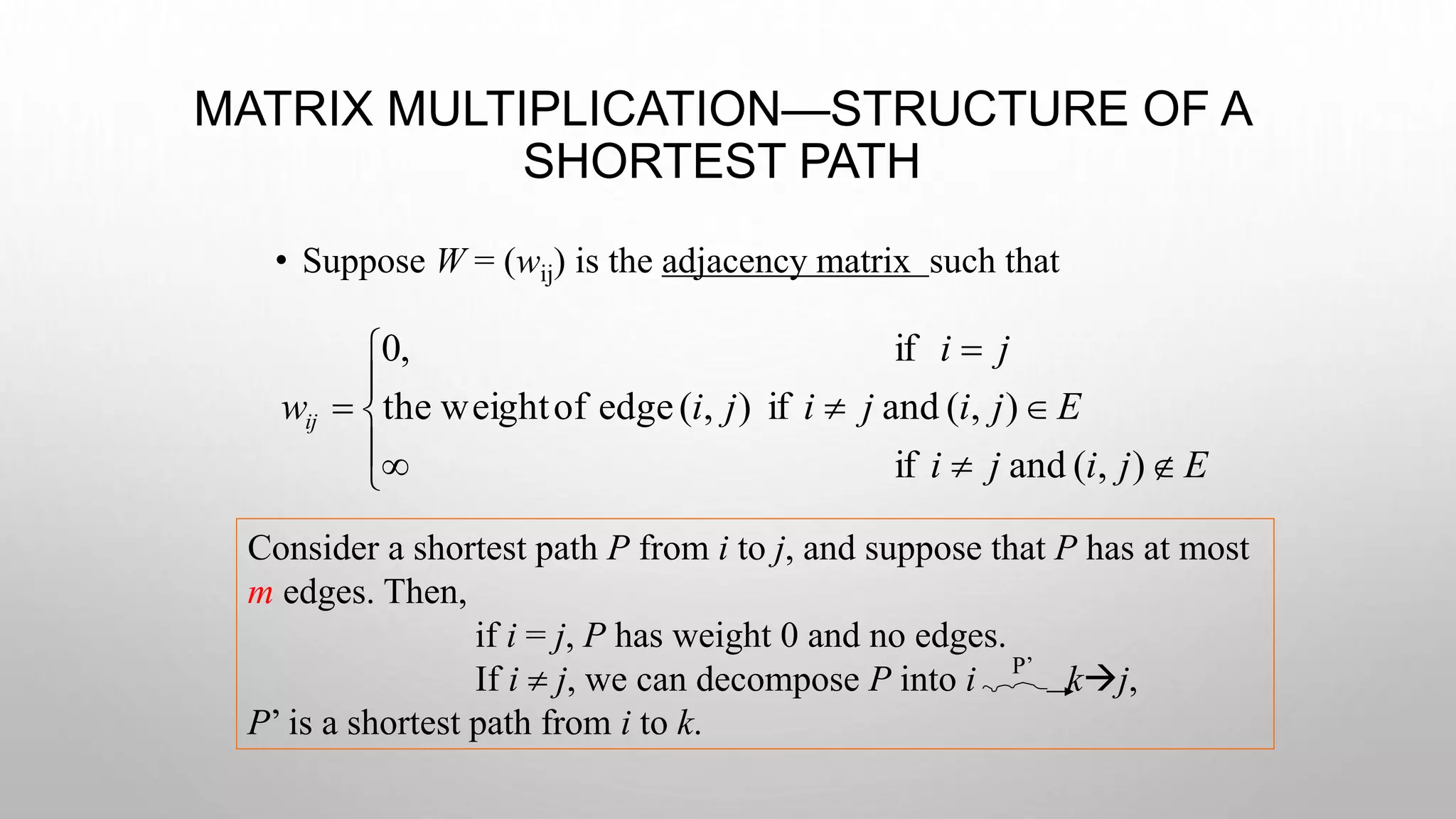
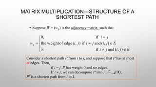
  MATRIX MULTIPLICATION—STRUCTURE OFA SHORTEST PATH • Suppose W = (wij) is the adjacency matrix such that          ),(andif ),(andif),(edgeofweightthe if,0 Ejiji Ejijiji ji wij Consider a shortest path P from i to j, and suppose that P has at most m edges. Then, if i = j, P has weight 0 and no edges. If i  j, we can decompose P into i kj, P’ is a shortest path from i to k. P’
• 11.
  FLOYD-WARSHALL ALGORITHM 5 1 2 3 4 3 4 -5 6 -42 1 8 7 k=1: d43 (1)＝-5; d42 (1)=5; d45 (1)= -2
• 12.
  FLOYD-WARSHALL ALGORITHM 5 1 2 3 4 3 4 -5 6 -42 1 8 7 k=2: d43 (2) =-5; d42 (2)=5; d45 (2)= 2
• 13.
  FLOYD-WARSHALL ALGORITHM 5 1 2 3 4 3 4 -5 6 -4 21 8 7 k=3: d42 (3)=-1; d43 (3)=-5; d45 (3)=-2
• 14.
  FLOYD-WARHSALL ALGORITHM (PSEUDO- CODE) Timecomplexity: O(n3)
• 15.
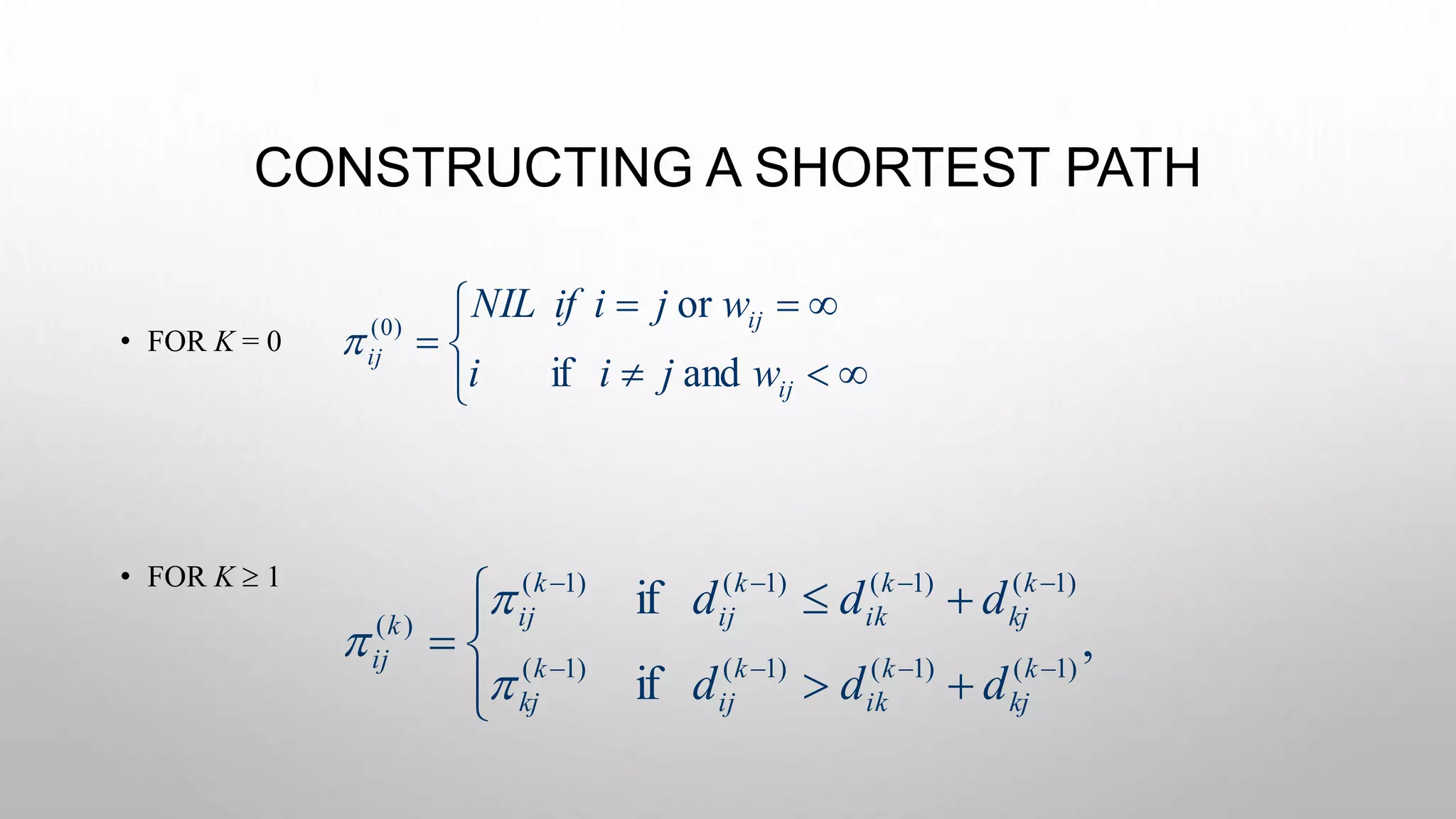
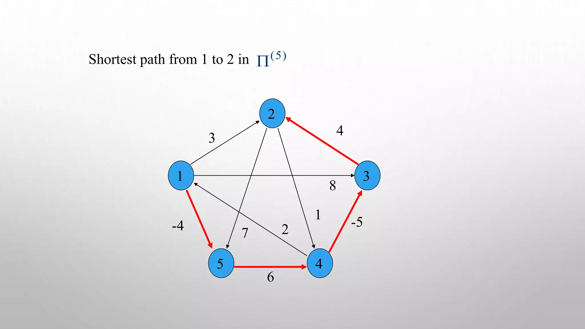
  CONSTRUCTING A SHORTESTPATH • FOR K = 0 • FOR K  1        ij ij ij wjii wjiifNIL andif or)0(  , if if )1()1()1()1( )1()1()1()1( )(          k kj k ik k ij k kj k kj k ik k ij k ijk ij ddd ddd   
• 16.
  PRINT ALL-PAIRS SHORTESTPATHS
• 17.
  EXAMPLE: 1 5 4 3 2 3 4 7 -4 8 1-5 2 6
• 18.
                       06 052 04 710 4830 D(0)=                 NILNILNILNIL NILNILNIL NILNILNILNIL NILNILNIL NILNIL 5 44 3 22 111 (0)= D(1)= (1)=                      06 20552 04 710 4830                   NILNILNILNIL NIL NILNILNILNIL NILNILNIL NILNIL 5 1414 3 22 111
• 19.
                       06 20552 11504 710 44830 D(2)=                 NILNILNILNIL NIL NILNIL NILNILNIL NIL 5 1414 223 22 1211 (2)= D(3)= (3)=                      06 20512 11504 710 44830                   NILNILNILNIL NIL NILNIL NILNILNIL NIL 5 1434 223 22 1211
• 20.
                     06158 20512 35047 11403 44130 D(4)=                 NIL NIL NIL NIL NIL 5434 1434 1234 1244 1241 (4)= D(5)= (5)=                    06158 20512 35047 11403 42310                   NIL NIL NIL NIL NIL 5434 1434 1234 1244 1543
• 21.
  1 5 4 3 2 3 4 7 -4 8 1-5 2 6 )5( Shortest path from 1 to 2 in