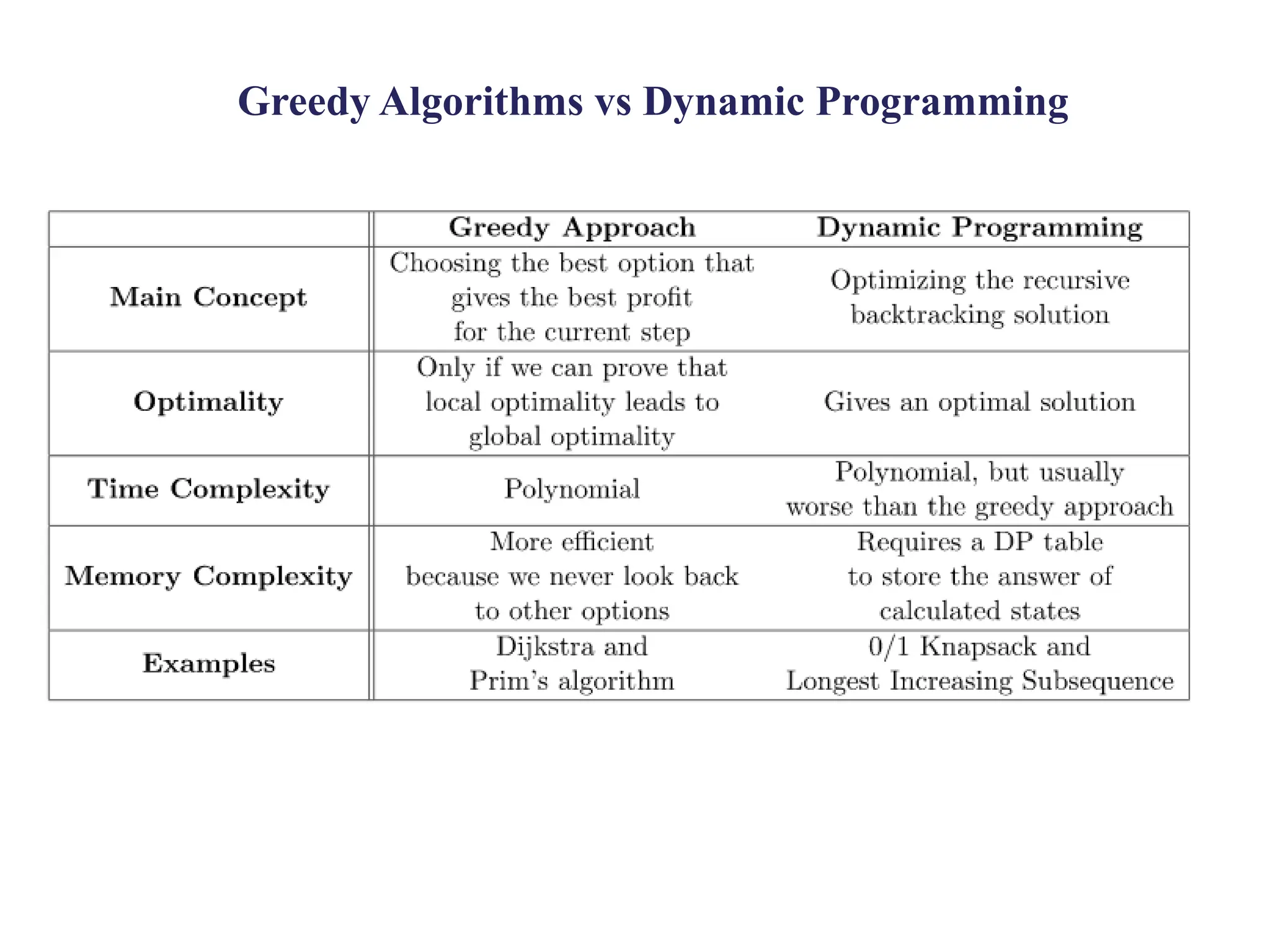
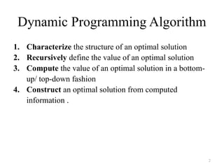
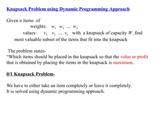
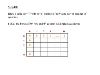
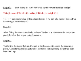
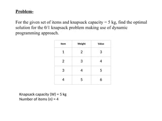
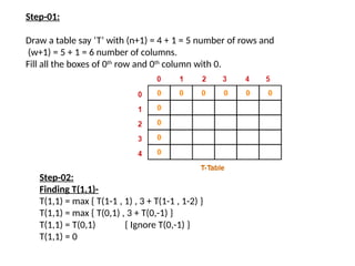
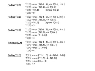
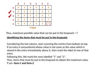
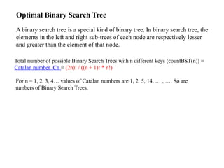
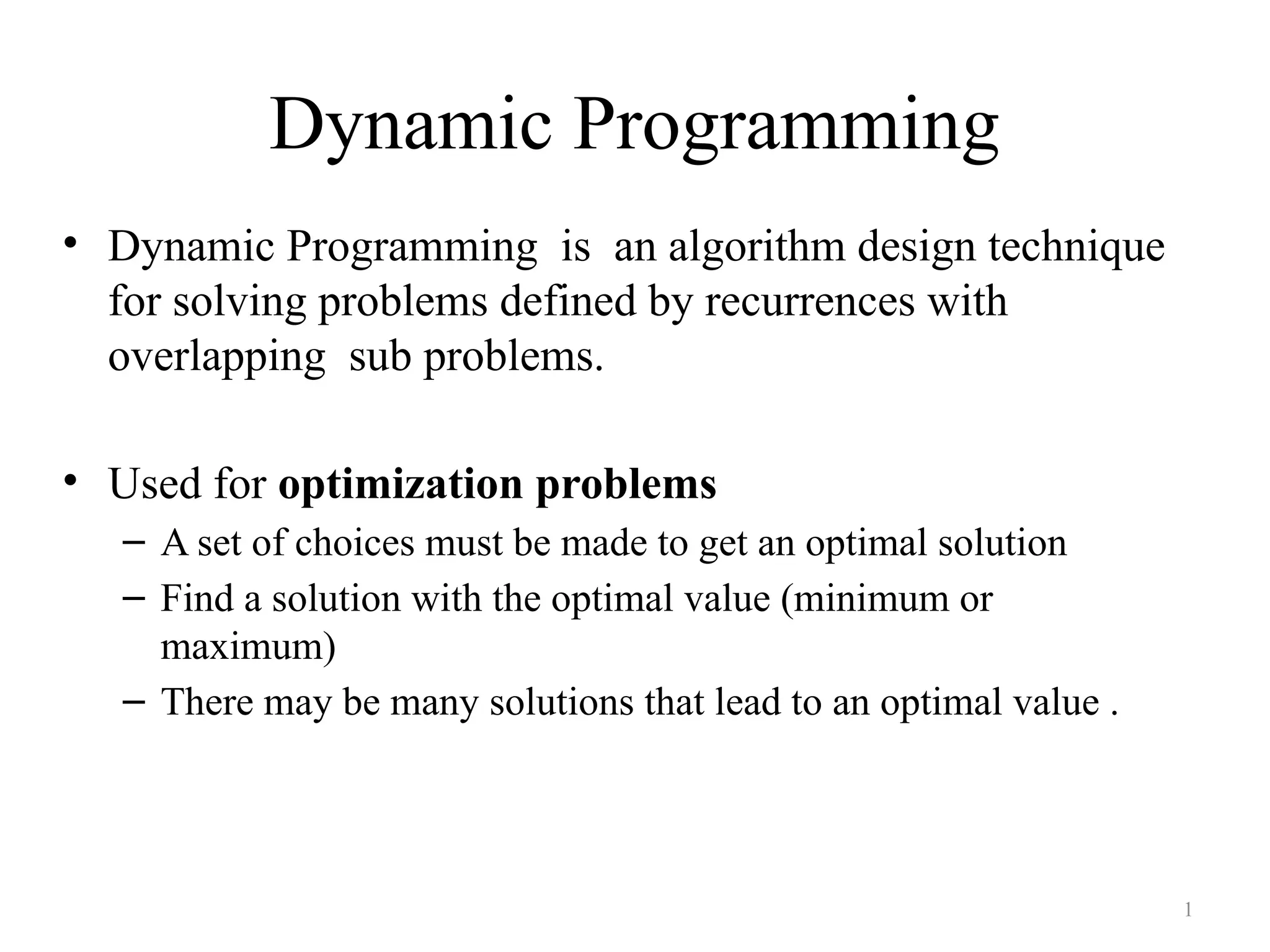
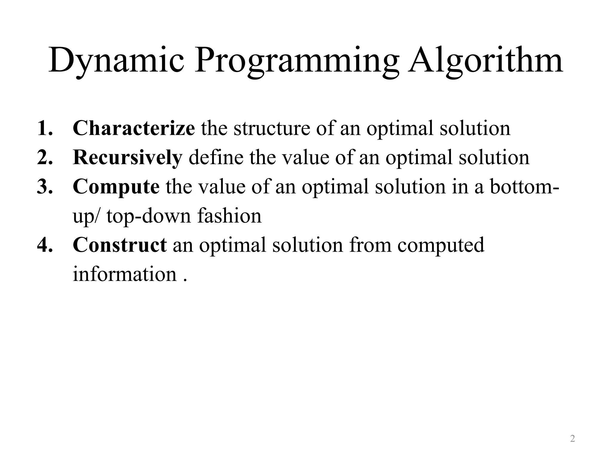
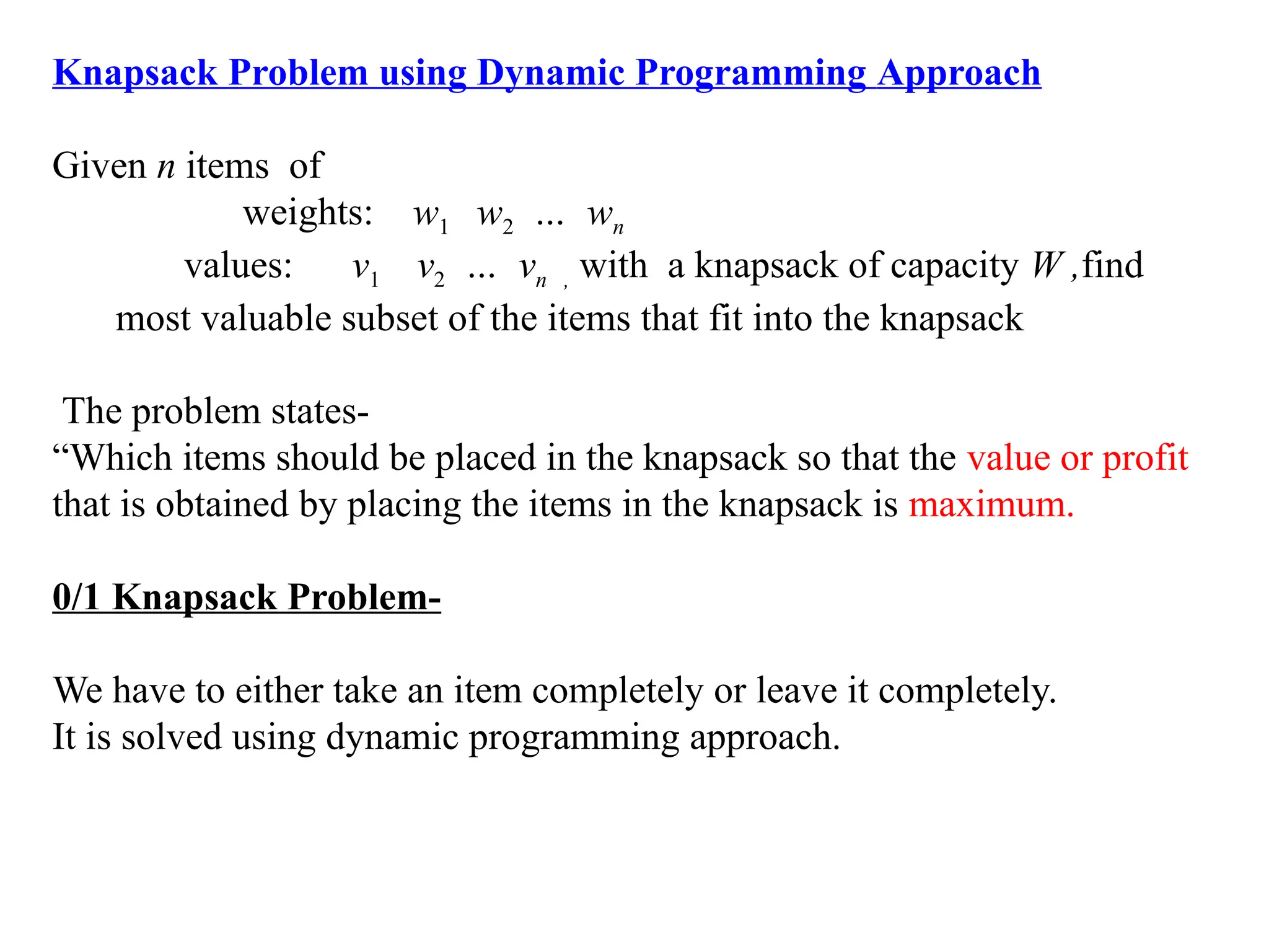
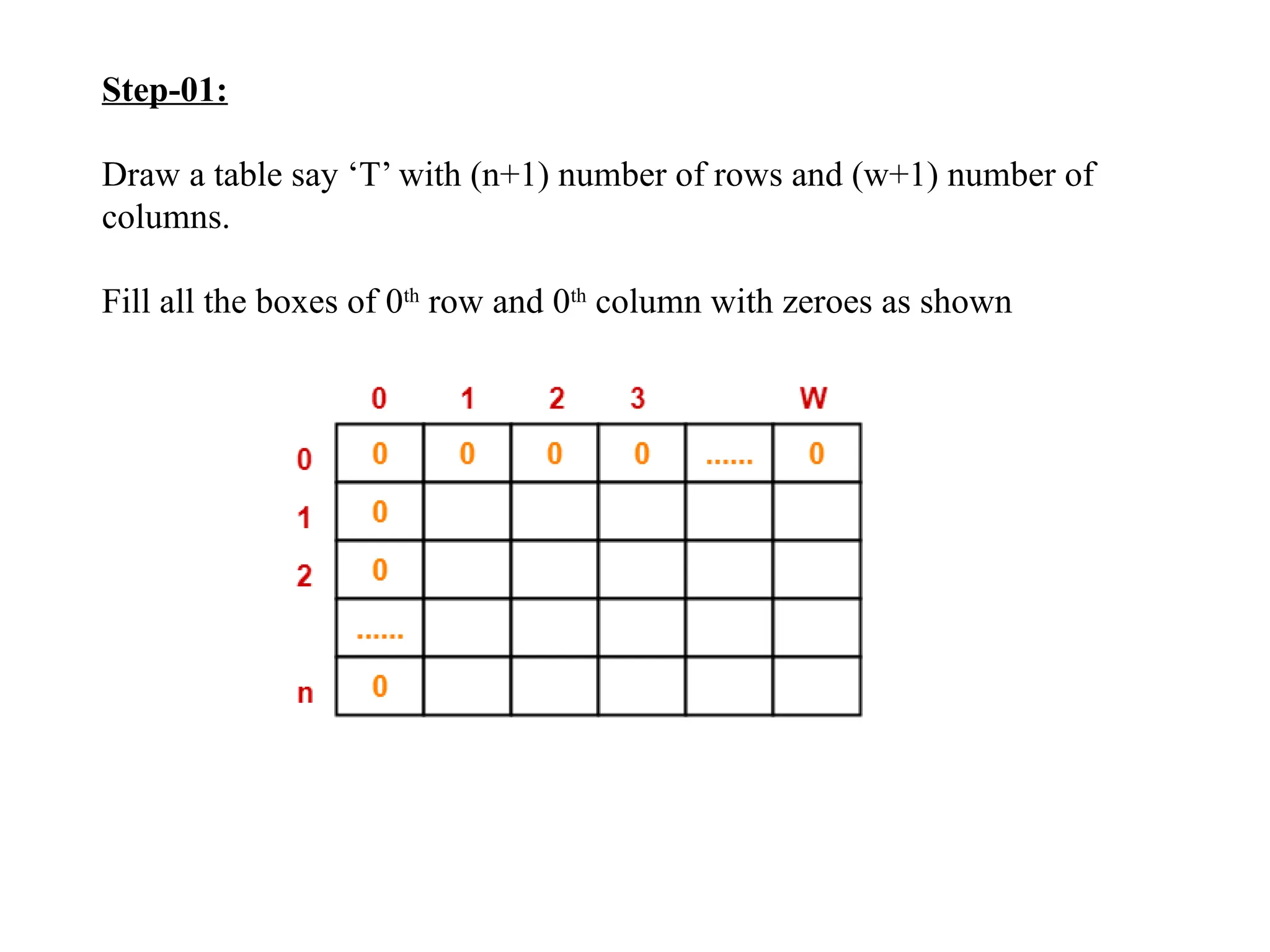
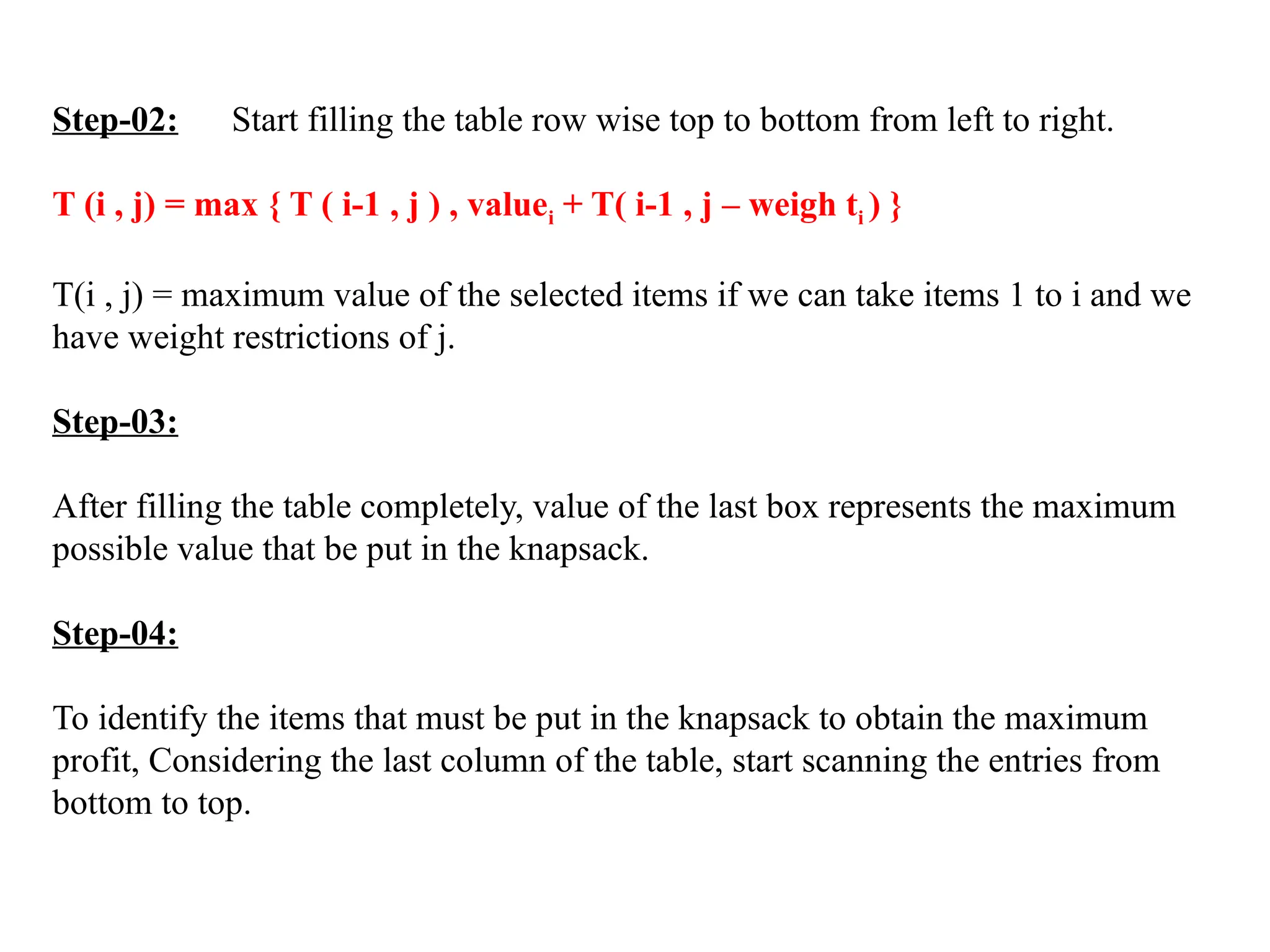
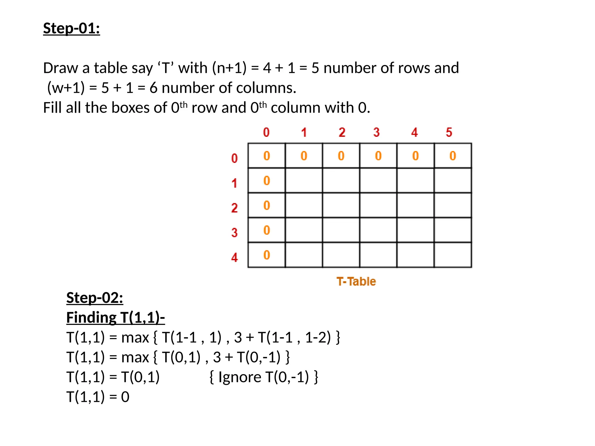
The document explains dynamic programming as an algorithm design technique for solving optimization problems, particularly highlighting the 0/1 knapsack problem and its variants. It also describes algorithms such as Floyd-Warshall for finding shortest paths in weighted graphs, and includes details on constructing optimal binary search trees and solving the traveling salesman problem. Various dynamic programming approaches and examples are provided to illustrate the concepts.


![All pairs shortest path problem(Floyd-Warshall Algorithm)
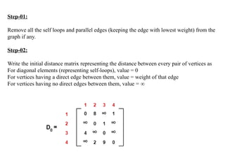
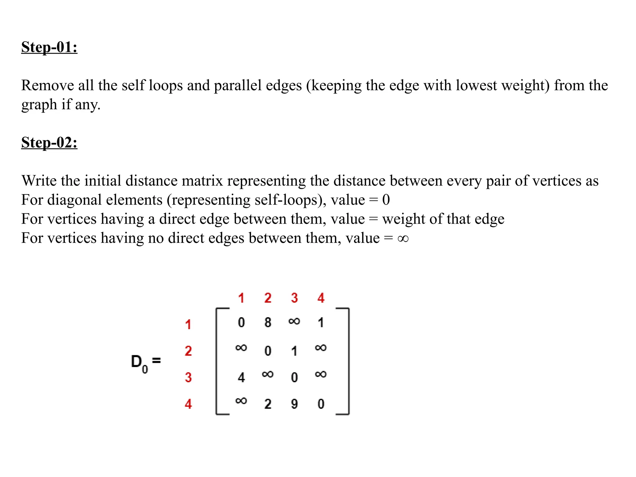
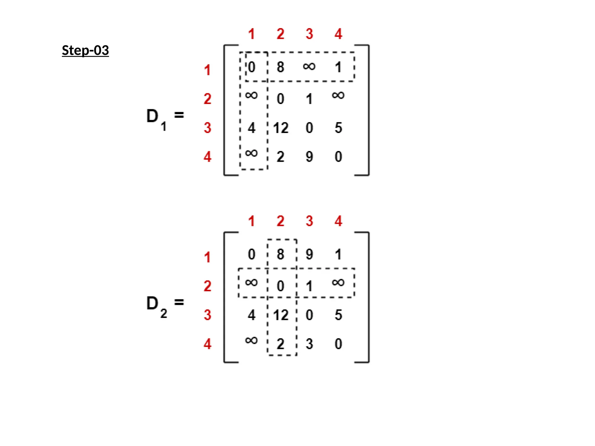
Floyd-Warshall algorithm is used to find all pair shortest paths from a given
weighted graph. As a result of this algorithm, it will generate a matrix, which will
represent the minimum distance from any node to all other nodes in the graph.
M[ i ][ j ] = 0 // For all diagonal elements, value = 0
If (i , j) is an edge in E, M[ i ][ j ] = weight(i,j)
// If there exists a direct edge between the vertices, value = weight of edge
Else
M[ i ][ j ] = infinity // If there is no direct edge between the vertices,
value = ∞](https://image.slidesharecdn.com/dynamicprogramming-240828073328-a31d1802/85/Dynamic-Programming-in-design-and-analysis-pptx-12-320.jpg)
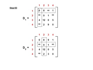
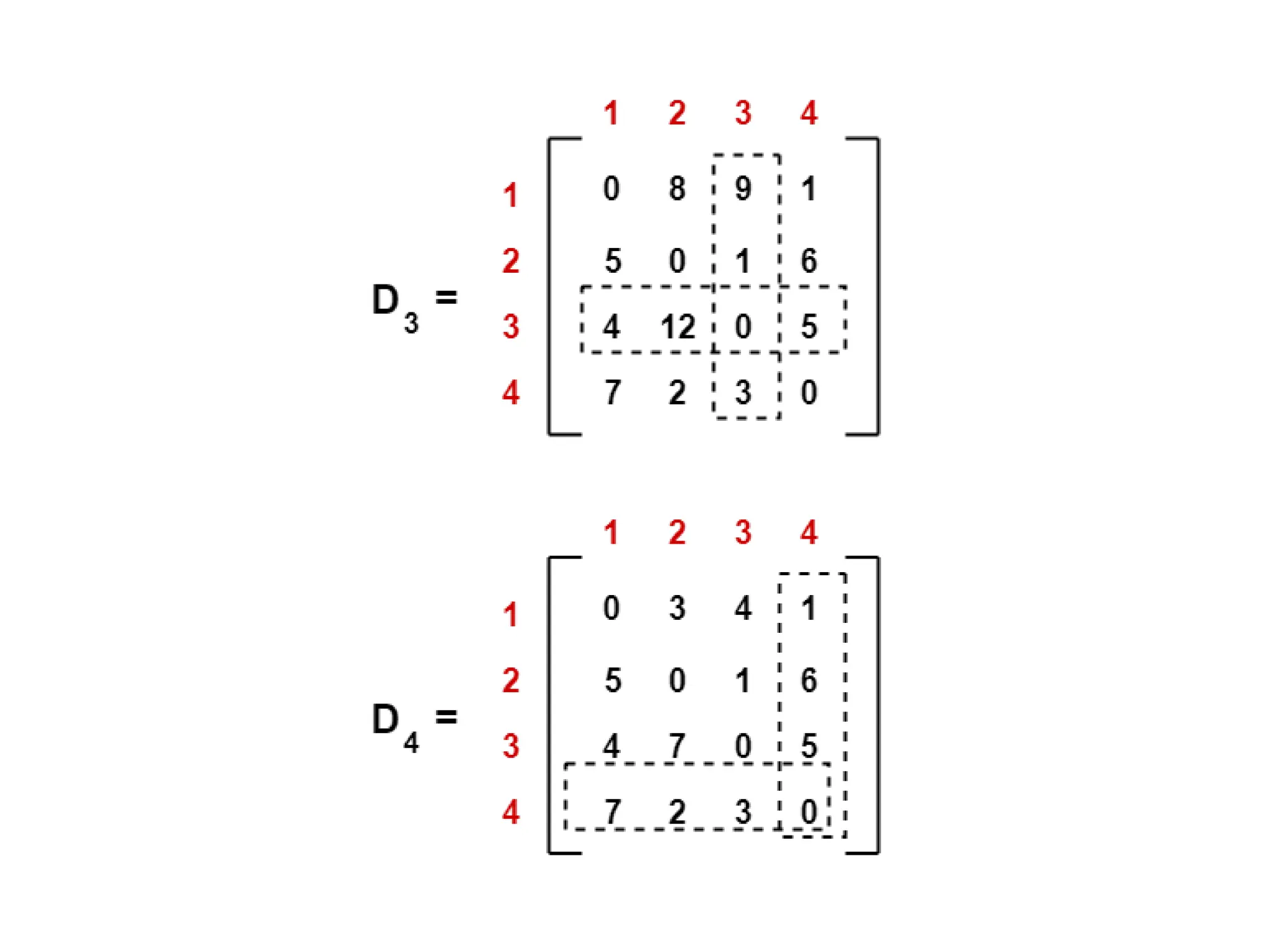
![for k from 1 to |V|
for i from 1 to |V|
for j from 1 to |V|
if M[ i ][ j ] > M[ i ][ k ] + M[ k ][ j ]
M[ i ][ j ] = M[ i ][ k ] + M[ k ][ j ]
The asymptotic complexity of Floyd-Warshall algorithm is O(n3
), here n is
the number of nodes in the given graph.](https://image.slidesharecdn.com/dynamicprogramming-240828073328-a31d1802/85/Dynamic-Programming-in-design-and-analysis-pptx-13-320.jpg)


![goal
0
0
C[i,j]
0
1
n+1
0 1 n
p 1
p2
n
p
i
j
C[i , j ]
Table :](https://image.slidesharecdn.com/dynamicprogramming-240828073328-a31d1802/85/Dynamic-Programming-in-design-and-analysis-pptx-21-320.jpg)
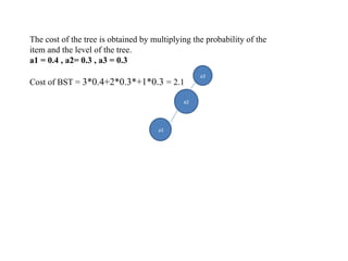
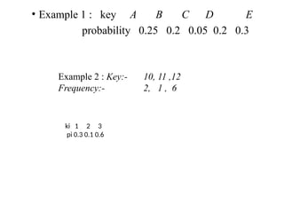
![Example: key A B C D
probability 0.1 0.2 0.4 0.3
The left table is filled using the recurrence
C[i, j] = min {C[i , k-1] + C[k+1 , j]} + ∑ ps , C[i ,i] = pi
The right saves the tree roots, which are the k’s that give the minimum
0 1 2 3 4
1 0 .1 .4 1.1 1.7
2 0 .2 .8 1.4
3 0 .4 1.0
4 0 .3
5 0
0 1 2 3 4
1 1 2 3 3
2 2 3 3
3 3 3
4 4
5
i ≤ k ≤ j s = i ≤ j
j
optimal BST
B
A
C
D
i
j
i
j](https://image.slidesharecdn.com/dynamicprogramming-240828073328-a31d1802/85/Dynamic-Programming-in-design-and-analysis-pptx-22-320.jpg)
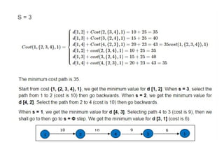
![S = Φ
Cost(2,Φ,1)=d(2,1)=5
Cost(3,Φ,1)=d(3,1)=6
Cost(4,Φ,1)=d(4,1)=8
S = 1
Cost(i,s)=min{Cost(j,s–(j))+d[i,j]}
Cost(2,{3},1)=d[2,3]+Cost(3,Φ,1)=9+6=15
Cost(2,{4},1)=d[2,4]+Cost(4,Φ,1)=10+8=18
Cost(3,{2},1)=d[3,2]+Cost(2,Φ,1)=13+5=18
Cost(3,{4},1)=d[3,4]+Cost(4,Φ,1)=12+8=20
cost(4,{2},1)=d[4,2]+cost(2,Φ,1)=8+5=13
Cost(4,{3},1)=d[4,3]+Cost(3,Φ,1)=9+6=15](https://image.slidesharecdn.com/dynamicprogramming-240828073328-a31d1802/85/Dynamic-Programming-in-design-and-analysis-pptx-25-320.jpg)
![Algorithm for Traveling salesman problem
Step 1: Let d[i, j] indicates the distance between cities i and j. Function
C[x, V – { x }]is the cost of the path starting from city x. V is the set of
cities/vertices in given graph. The aim of TSP is to minimize the cost
function.
Step 2: Assume that graph contains n vertices V1, V2, ..., Vn. TSP
finds a path covering all vertices exactly once, and the same time it
tries to minimize the overall traveling distance.
Step 3: Mathematical formula to find minimum distance is stated
below: C(i, V) = min { d[i, j] + C(j, V – { j }) }, j V and i V. TSP
∈ ∉
problem possesses the principle of optimality, i.e. for d[V1, Vn] to be
minimum, any intermediate path (Vi, Vj) must be minimum.](https://image.slidesharecdn.com/dynamicprogramming-240828073328-a31d1802/85/Dynamic-Programming-in-design-and-analysis-pptx-28-320.jpg)
![– 24 11 10 9
8 – 2 5 11
26 12 – 8 7
11 23 24 – 6
5 4 8 11 –
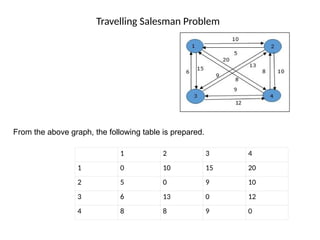
Problem: Solve the traveling salesman problem with the associated cost adjacency matrix
using dynamic programming.
Solution:
Let us start our tour from city 1.
Step 1: Initially, we will find the distance between city 1 and city {2, 3, 4, 5}
without visiting any intermediate city.
Cost(x, y, z) represents the distance from x to z and y as an intermediate city.
Cost(2, Φ, 1) = d[2, 1] = 24
Cost(3, Φ, 1) = d[3, 1] = 11
Cost(4, Φ , 1) = d[4, 1] = 10
Cost(5, Φ , 1) = d[5, 1] = 9](https://image.slidesharecdn.com/dynamicprogramming-240828073328-a31d1802/85/Dynamic-Programming-in-design-and-analysis-pptx-29-320.jpg)
![Step 2: In this step, we will find the minimum distance by visiting 1 city as
intermediate city.
Cost{2, {3}, 1} = d[2, 3] + Cost(3, Φ, 1) = 2 + 11 = 13
Cost{2, {4}, 1} = d[2, 4] + Cost(4, Φ, 1) = 5 + 10 = 15
Cost{2, {5}, 1} = d[2, 5] + Cost(5, Φ, 1) = 11 + 9 = 20
Cost{3, {2}, 1} = d[3, 2] + Cost(2, Φ, 1) = 12 + 24 = 36
Cost{3, {4}, 1} = d[3, 4] + Cost(4, Φ, 1) = 8 + 10 = 18
Cost{3, {5}, 1} = d[3, 5] + Cost(5, Φ, 1) = 7 + 9 = 16
Cost{4, {2}, 1} = d[4, 2] + Cost(2, Φ, 1) = 23 + 24 = 47
Cost{4, {3}, 1} = d[4, 3] + Cost(3, Φ, 1) = 24 + 11 = 35
Cost{4, {5}, 1} = d[4, 5] + Cost(5, Φ, 1) = 6 + 9 = 15
Cost{5, {2}, 1} = d[5, 2] + Cost(2, Φ, 1) = 4 + 24 = 28
Cost{5, {3}, 1} = d[5, 3] + Cost(3, Φ, 1) = 8 + 11 = 19
Cost{5, {4}, 1} = d[5, 4] + Cost(4, Φ, 1) = 11 + 10 = 21](https://image.slidesharecdn.com/dynamicprogramming-240828073328-a31d1802/85/Dynamic-Programming-in-design-and-analysis-pptx-30-320.jpg)
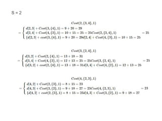
![Step 3: In this step, we will find the minimum distance by visiting 2 cities as intermediate city.
Cost(2, {3, 4}, 1) = min { d[2, 3] + Cost(3, {4}, 1), d[2, 4] + Cost(4, {3}, 1)]}
= min { [2 + 18], [5 + 35] } = min{20, 40} = 20
Cost(2, {4, 5}, 1) = min { d[2, 4] + Cost(4, {5}, 1), d[2, 5] + Cost(5, {4}, 1)]}
= min { [5 + 15], [11 + 21] } = min{20, 32} = 20
Cost(2, {3, 5}, 1) = min { d[2, 3] + Cost(3, {4}, 1), d[2, 4] + Cost(4, {3}, 1)]}
= min { [2 + 18], [5 + 35] } = min{20, 40} = 20
Cost(3, {2, 4}, 1) = min { d[3, 2] + Cost(2, {4}, 1), d[3, 4] + Cost(4, {2}, 1)]}
= min { [12 + 15], [8 + 47] } = min{27, 55} = 27
Cost(3, {4, 5}, 1) = min { d[3, 4] + Cost(4, {5}, 1), d[3, 5] + Cost(5, {4}, 1)]}
= min { [8 + 15], [7 + 21] } = min{23, 28} = 23
Cost(3, {2, 5}, 1) = min { d[3, 2] + Cost(2, {5}, 1), d[3, 5] + Cost(5, {2}, 1)]}
= min { [12 + 20], [7 + 28] } = min{32, 35} = 32
Cost(4, {2, 3}, 1) = min{ d[4, 2] + Cost(2, {3}, 1), d[4, 3] + Cost(3, {2}, 1)]}
= min { [23 + 13], [24 + 36] } = min{36, 60} = 36
Cost(4, {3, 5}, 1) = min{ d[4, 3] + Cost(3, {5}, 1), d[4, 5] + Cost(5, {3}, 1)]}
= min { [24 + 16], [6 + 19] } = min{40, 25} = 25
Cost(4, {2, 5}, 1) = min{ d[4, 2] + Cost(2, {5}, 1), d[4, 5] + Cost(5, {2}, 1)]}
= min { [23 + 20], [6 + 28] } = min{43, 34} = 34
Cost(5, {2, 3}, 1) = min{ d[5, 2] + Cost(2, {3}, 1), d[5, 3] + Cost(3, {2}, 1)]}
= min { [4 + 13], [8 + 36] } = min{17, 44} = 17
Cost(5, {3, 4}, 1) = min{ d[5, 3] + Cost(3, {4}, 1), d[5, 4] + Cost(4, {3}, 1)]}
= min { [8 + 18], [11 + 35] } = min{26, 46} = 26
Cost(5, {2, 4}, 1) = min{ d[5, 2] + Cost(2, {4}, 1), d[5, 4] + Cost(4, {2}, 1)]}
= min { [4 + 15], [11 + 47] } = min{19, 58} = 19](https://image.slidesharecdn.com/dynamicprogramming-240828073328-a31d1802/85/Dynamic-Programming-in-design-and-analysis-pptx-31-320.jpg)
![Step 4 : In this step, we will find the minimum distance by visiting 3 cities as
intermediate city.
Cost(2, {3, 4, 5}, 1) = min d[2, 3] + Cost(3, {4, 5}, 1)
d[2, 4] + Cost(4, {3, 5}, 1)
d[2, 5] + Cost(5, {3, 4}, 1)
= min { 2 + 23, 5 + 25, 11 + 36}
= min{25, 30, 47} = 25
Cost(3, {2, 4, 5}, 1) = min d[3, 2] + Cost(2, {4, 5}, 1)
d[3, 4] + Cost(4, {2, 5}, 1)
d[3, 5] + Cost(5, {2, 4}, 1)
= min { 12 + 20, 8 + 34, 7 + 19}
= min{32, 42, 26} = 26
Cost(4, {2, 3, 5}, 1) = min d[4, 2] + Cost(2, {3, 5}, 1)
d[4, 3] + Cost(3, {2, 5}, 1)
d[4, 5] + Cost(5, {2, 3}, 1)
= min {23 + 30, 24 + 32, 6 + 17}
= min{53, 56, 23} = 23
Cost(5, {2, 3, 4}, 1) = min d[5, 2] + Cost(2, {3, 4}, 1)
d[5, 3] + Cost(3, {2, 4}, 1)
d[5, 4] + Cost(4, {2, 3}, 1)
= min {4 + 30, 8 + 27, 11 + 36}
= min{34, 35, 47} = 34](https://image.slidesharecdn.com/dynamicprogramming-240828073328-a31d1802/85/Dynamic-Programming-in-design-and-analysis-pptx-32-320.jpg)
![Step 5 : In this step, we will find the minimum distance by visiting 4 cities
as an intermediate city.
Cost(1, {2, 3, 4, 5}, 1) = min d[1, 2] + Cost(2, {3, 4, 5}, 1)
d[1, 3] + Cost(3, {2, 4, 5}, 1)
d[1, 4] + Cost(4, {2, 3, 5}, 1)
d[1, 5] + Cost(5, {2, 3, 4}, 1)
= min { 24 + 25, 11 + 26, 10 + 23, 9 + 34 }
= min{49, 37, 33, 43} = 33
Thus, minimum length tour would be of 33.](https://image.slidesharecdn.com/dynamicprogramming-240828073328-a31d1802/85/Dynamic-Programming-in-design-and-analysis-pptx-33-320.jpg)
![Trace the path:
Let us find the path that gives the distance of 33.
Cost(1, {2, 3, 4, 5}, 1) is minimum due to d[1, 4], so move from 1 to 4. Path = {1, 4}.
Cost(4, {2, 3, 5}, 1) is minimum due to d[4, 5], so move from 4 to 5. Path = {1, 4, 5}.
Cost(5, {2, 3}, 1) is minimum due to d[5, 2], so move from 5 to 2. Path = {1, 4, 5, 2}.
Cost(2, {3}, 1) is minimum due to d[2, 3], so move from 2 to 3. Path = {1, 4, 5, 2, 3}.
All cities are visited so come back to 1. Hence the optimum tour would be
1 – 4 – 5 – 2 – 3 – 1.](https://image.slidesharecdn.com/dynamicprogramming-240828073328-a31d1802/85/Dynamic-Programming-in-design-and-analysis-pptx-34-320.jpg)


![All pairs shortest path problem(Floyd-Warshall Algorithm)
Floyd-Warshall algorithm is used to find all pair shortest paths from a given
weighted graph. As a result of this algorithm, it will generate a matrix, which will
represent the minimum distance from any node to all other nodes in the graph.
M[ i ][ j ] = 0 // For all diagonal elements, value = 0
If (i , j) is an edge in E, M[ i ][ j ] = weight(i,j)
// If there exists a direct edge between the vertices, value = weight of edge
Else
M[ i ][ j ] = infinity // If there is no direct edge between the vertices,
value = ∞](https://image.slidesharecdn.com/dynamicprogramming-240828073328-a31d1802/75/Dynamic-Programming-in-design-and-analysis-pptx-12-2048.jpg)
![for k from 1 to |V|
for i from 1 to |V|
for j from 1 to |V|
if M[ i ][ j ] > M[ i ][ k ] + M[ k ][ j ]
M[ i ][ j ] = M[ i ][ k ] + M[ k ][ j ]
The asymptotic complexity of Floyd-Warshall algorithm is O(n3
), here n is
the number of nodes in the given graph.](https://image.slidesharecdn.com/dynamicprogramming-240828073328-a31d1802/75/Dynamic-Programming-in-design-and-analysis-pptx-13-2048.jpg)


![goal
0
0
C[i,j]
0
1
n+1
0 1 n
p 1
p2
n
p
i
j
C[i , j ]
Table :](https://image.slidesharecdn.com/dynamicprogramming-240828073328-a31d1802/75/Dynamic-Programming-in-design-and-analysis-pptx-21-2048.jpg)
![Example: key A B C D
probability 0.1 0.2 0.4 0.3
The left table is filled using the recurrence
C[i, j] = min {C[i , k-1] + C[k+1 , j]} + ∑ ps , C[i ,i] = pi
The right saves the tree roots, which are the k’s that give the minimum
0 1 2 3 4
1 0 .1 .4 1.1 1.7
2 0 .2 .8 1.4
3 0 .4 1.0
4 0 .3
5 0
0 1 2 3 4
1 1 2 3 3
2 2 3 3
3 3 3
4 4
5
i ≤ k ≤ j s = i ≤ j
j
optimal BST
B
A
C
D
i
j
i
j](https://image.slidesharecdn.com/dynamicprogramming-240828073328-a31d1802/75/Dynamic-Programming-in-design-and-analysis-pptx-22-2048.jpg)


![S = Φ
Cost(2,Φ,1)=d(2,1)=5
Cost(3,Φ,1)=d(3,1)=6
Cost(4,Φ,1)=d(4,1)=8
S = 1
Cost(i,s)=min{Cost(j,s–(j))+d[i,j]}
Cost(2,{3},1)=d[2,3]+Cost(3,Φ,1)=9+6=15
Cost(2,{4},1)=d[2,4]+Cost(4,Φ,1)=10+8=18
Cost(3,{2},1)=d[3,2]+Cost(2,Φ,1)=13+5=18
Cost(3,{4},1)=d[3,4]+Cost(4,Φ,1)=12+8=20
cost(4,{2},1)=d[4,2]+cost(2,Φ,1)=8+5=13
Cost(4,{3},1)=d[4,3]+Cost(3,Φ,1)=9+6=15](https://image.slidesharecdn.com/dynamicprogramming-240828073328-a31d1802/75/Dynamic-Programming-in-design-and-analysis-pptx-25-2048.jpg)

![Algorithm for Traveling salesman problem
Step 1: Let d[i, j] indicates the distance between cities i and j. Function
C[x, V – { x }]is the cost of the path starting from city x. V is the set of
cities/vertices in given graph. The aim of TSP is to minimize the cost
function.
Step 2: Assume that graph contains n vertices V1, V2, ..., Vn. TSP
finds a path covering all vertices exactly once, and the same time it
tries to minimize the overall traveling distance.
Step 3: Mathematical formula to find minimum distance is stated
below: C(i, V) = min { d[i, j] + C(j, V – { j }) }, j V and i V. TSP
∈ ∉
problem possesses the principle of optimality, i.e. for d[V1, Vn] to be
minimum, any intermediate path (Vi, Vj) must be minimum.](https://image.slidesharecdn.com/dynamicprogramming-240828073328-a31d1802/75/Dynamic-Programming-in-design-and-analysis-pptx-28-2048.jpg)
![– 24 11 10 9
8 – 2 5 11
26 12 – 8 7
11 23 24 – 6
5 4 8 11 –
Problem: Solve the traveling salesman problem with the associated cost adjacency matrix
using dynamic programming.
Solution:
Let us start our tour from city 1.
Step 1: Initially, we will find the distance between city 1 and city {2, 3, 4, 5}
without visiting any intermediate city.
Cost(x, y, z) represents the distance from x to z and y as an intermediate city.
Cost(2, Φ, 1) = d[2, 1] = 24
Cost(3, Φ, 1) = d[3, 1] = 11
Cost(4, Φ , 1) = d[4, 1] = 10
Cost(5, Φ , 1) = d[5, 1] = 9](https://image.slidesharecdn.com/dynamicprogramming-240828073328-a31d1802/75/Dynamic-Programming-in-design-and-analysis-pptx-29-2048.jpg)
![Step 2: In this step, we will find the minimum distance by visiting 1 city as
intermediate city.
Cost{2, {3}, 1} = d[2, 3] + Cost(3, Φ, 1) = 2 + 11 = 13
Cost{2, {4}, 1} = d[2, 4] + Cost(4, Φ, 1) = 5 + 10 = 15
Cost{2, {5}, 1} = d[2, 5] + Cost(5, Φ, 1) = 11 + 9 = 20
Cost{3, {2}, 1} = d[3, 2] + Cost(2, Φ, 1) = 12 + 24 = 36
Cost{3, {4}, 1} = d[3, 4] + Cost(4, Φ, 1) = 8 + 10 = 18
Cost{3, {5}, 1} = d[3, 5] + Cost(5, Φ, 1) = 7 + 9 = 16
Cost{4, {2}, 1} = d[4, 2] + Cost(2, Φ, 1) = 23 + 24 = 47
Cost{4, {3}, 1} = d[4, 3] + Cost(3, Φ, 1) = 24 + 11 = 35
Cost{4, {5}, 1} = d[4, 5] + Cost(5, Φ, 1) = 6 + 9 = 15
Cost{5, {2}, 1} = d[5, 2] + Cost(2, Φ, 1) = 4 + 24 = 28
Cost{5, {3}, 1} = d[5, 3] + Cost(3, Φ, 1) = 8 + 11 = 19
Cost{5, {4}, 1} = d[5, 4] + Cost(4, Φ, 1) = 11 + 10 = 21](https://image.slidesharecdn.com/dynamicprogramming-240828073328-a31d1802/75/Dynamic-Programming-in-design-and-analysis-pptx-30-2048.jpg)
![Step 3: In this step, we will find the minimum distance by visiting 2 cities as intermediate city.
Cost(2, {3, 4}, 1) = min { d[2, 3] + Cost(3, {4}, 1), d[2, 4] + Cost(4, {3}, 1)]}
= min { [2 + 18], [5 + 35] } = min{20, 40} = 20
Cost(2, {4, 5}, 1) = min { d[2, 4] + Cost(4, {5}, 1), d[2, 5] + Cost(5, {4}, 1)]}
= min { [5 + 15], [11 + 21] } = min{20, 32} = 20
Cost(2, {3, 5}, 1) = min { d[2, 3] + Cost(3, {4}, 1), d[2, 4] + Cost(4, {3}, 1)]}
= min { [2 + 18], [5 + 35] } = min{20, 40} = 20
Cost(3, {2, 4}, 1) = min { d[3, 2] + Cost(2, {4}, 1), d[3, 4] + Cost(4, {2}, 1)]}
= min { [12 + 15], [8 + 47] } = min{27, 55} = 27
Cost(3, {4, 5}, 1) = min { d[3, 4] + Cost(4, {5}, 1), d[3, 5] + Cost(5, {4}, 1)]}
= min { [8 + 15], [7 + 21] } = min{23, 28} = 23
Cost(3, {2, 5}, 1) = min { d[3, 2] + Cost(2, {5}, 1), d[3, 5] + Cost(5, {2}, 1)]}
= min { [12 + 20], [7 + 28] } = min{32, 35} = 32
Cost(4, {2, 3}, 1) = min{ d[4, 2] + Cost(2, {3}, 1), d[4, 3] + Cost(3, {2}, 1)]}
= min { [23 + 13], [24 + 36] } = min{36, 60} = 36
Cost(4, {3, 5}, 1) = min{ d[4, 3] + Cost(3, {5}, 1), d[4, 5] + Cost(5, {3}, 1)]}
= min { [24 + 16], [6 + 19] } = min{40, 25} = 25
Cost(4, {2, 5}, 1) = min{ d[4, 2] + Cost(2, {5}, 1), d[4, 5] + Cost(5, {2}, 1)]}
= min { [23 + 20], [6 + 28] } = min{43, 34} = 34
Cost(5, {2, 3}, 1) = min{ d[5, 2] + Cost(2, {3}, 1), d[5, 3] + Cost(3, {2}, 1)]}
= min { [4 + 13], [8 + 36] } = min{17, 44} = 17
Cost(5, {3, 4}, 1) = min{ d[5, 3] + Cost(3, {4}, 1), d[5, 4] + Cost(4, {3}, 1)]}
= min { [8 + 18], [11 + 35] } = min{26, 46} = 26
Cost(5, {2, 4}, 1) = min{ d[5, 2] + Cost(2, {4}, 1), d[5, 4] + Cost(4, {2}, 1)]}
= min { [4 + 15], [11 + 47] } = min{19, 58} = 19](https://image.slidesharecdn.com/dynamicprogramming-240828073328-a31d1802/75/Dynamic-Programming-in-design-and-analysis-pptx-31-2048.jpg)
![Step 4 : In this step, we will find the minimum distance by visiting 3 cities as
intermediate city.
Cost(2, {3, 4, 5}, 1) = min d[2, 3] + Cost(3, {4, 5}, 1)
d[2, 4] + Cost(4, {3, 5}, 1)
d[2, 5] + Cost(5, {3, 4}, 1)
= min { 2 + 23, 5 + 25, 11 + 36}
= min{25, 30, 47} = 25
Cost(3, {2, 4, 5}, 1) = min d[3, 2] + Cost(2, {4, 5}, 1)
d[3, 4] + Cost(4, {2, 5}, 1)
d[3, 5] + Cost(5, {2, 4}, 1)
= min { 12 + 20, 8 + 34, 7 + 19}
= min{32, 42, 26} = 26
Cost(4, {2, 3, 5}, 1) = min d[4, 2] + Cost(2, {3, 5}, 1)
d[4, 3] + Cost(3, {2, 5}, 1)
d[4, 5] + Cost(5, {2, 3}, 1)
= min {23 + 30, 24 + 32, 6 + 17}
= min{53, 56, 23} = 23
Cost(5, {2, 3, 4}, 1) = min d[5, 2] + Cost(2, {3, 4}, 1)
d[5, 3] + Cost(3, {2, 4}, 1)
d[5, 4] + Cost(4, {2, 3}, 1)
= min {4 + 30, 8 + 27, 11 + 36}
= min{34, 35, 47} = 34](https://image.slidesharecdn.com/dynamicprogramming-240828073328-a31d1802/75/Dynamic-Programming-in-design-and-analysis-pptx-32-2048.jpg)
![Step 5 : In this step, we will find the minimum distance by visiting 4 cities
as an intermediate city.
Cost(1, {2, 3, 4, 5}, 1) = min d[1, 2] + Cost(2, {3, 4, 5}, 1)
d[1, 3] + Cost(3, {2, 4, 5}, 1)
d[1, 4] + Cost(4, {2, 3, 5}, 1)
d[1, 5] + Cost(5, {2, 3, 4}, 1)
= min { 24 + 25, 11 + 26, 10 + 23, 9 + 34 }
= min{49, 37, 33, 43} = 33
Thus, minimum length tour would be of 33.](https://image.slidesharecdn.com/dynamicprogramming-240828073328-a31d1802/75/Dynamic-Programming-in-design-and-analysis-pptx-33-2048.jpg)
![Trace the path:
Let us find the path that gives the distance of 33.
Cost(1, {2, 3, 4, 5}, 1) is minimum due to d[1, 4], so move from 1 to 4. Path = {1, 4}.
Cost(4, {2, 3, 5}, 1) is minimum due to d[4, 5], so move from 4 to 5. Path = {1, 4, 5}.
Cost(5, {2, 3}, 1) is minimum due to d[5, 2], so move from 5 to 2. Path = {1, 4, 5, 2}.
Cost(2, {3}, 1) is minimum due to d[2, 3], so move from 2 to 3. Path = {1, 4, 5, 2, 3}.
All cities are visited so come back to 1. Hence the optimum tour would be
1 – 4 – 5 – 2 – 3 – 1.](https://image.slidesharecdn.com/dynamicprogramming-240828073328-a31d1802/75/Dynamic-Programming-in-design-and-analysis-pptx-34-2048.jpg)