Download as PDF, PPTX

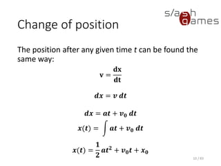
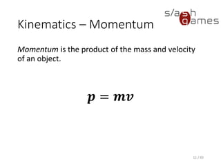
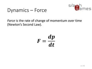
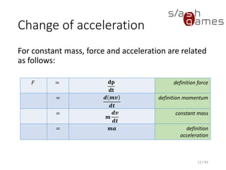
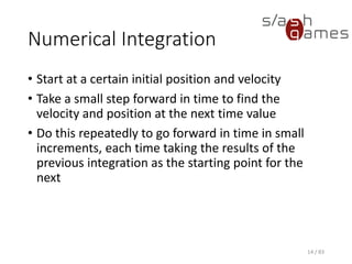
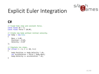
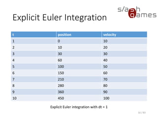
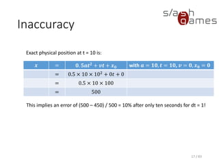
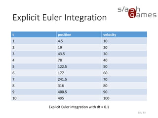
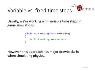
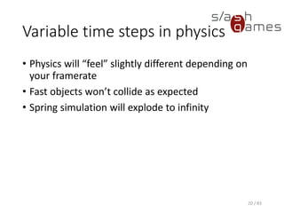
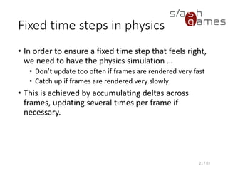
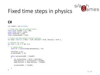
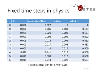
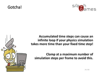
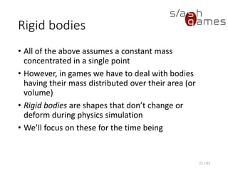
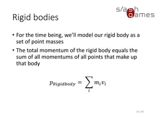
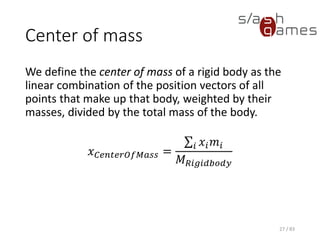
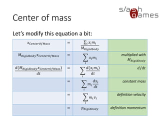

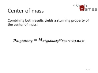
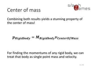
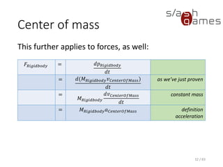
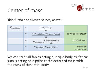
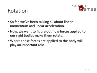
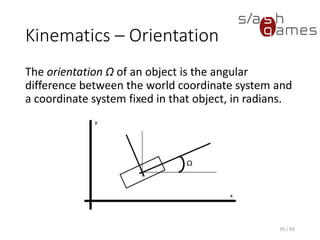
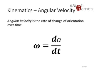
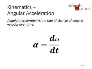
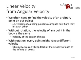


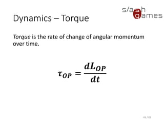

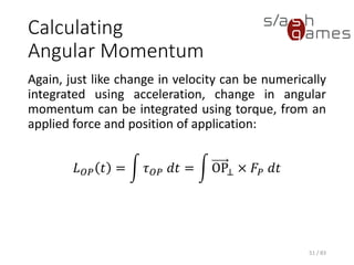
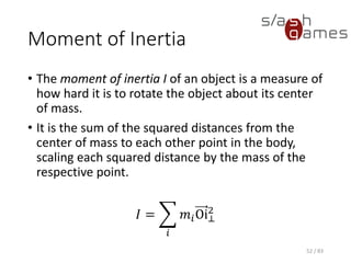
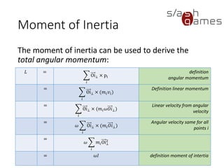

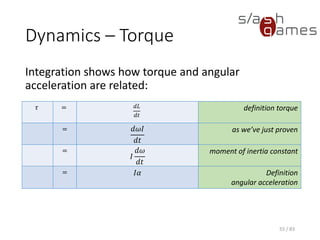
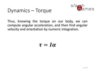
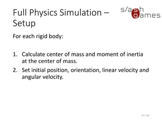
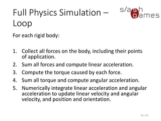

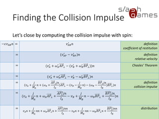

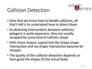
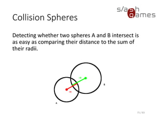

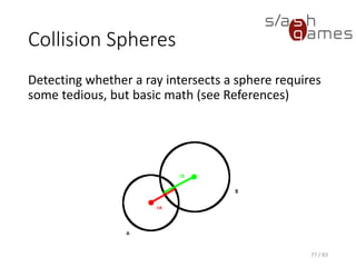


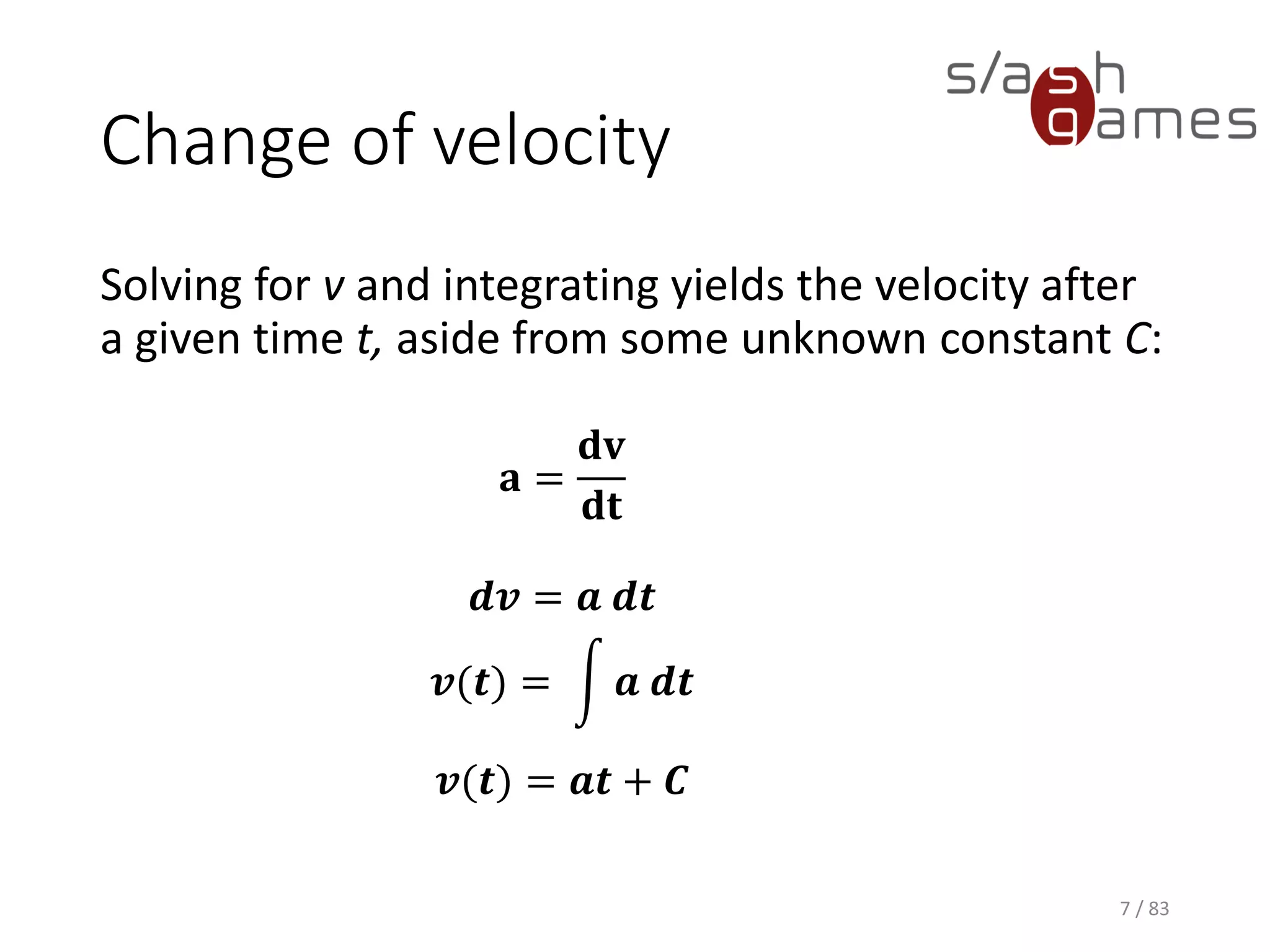
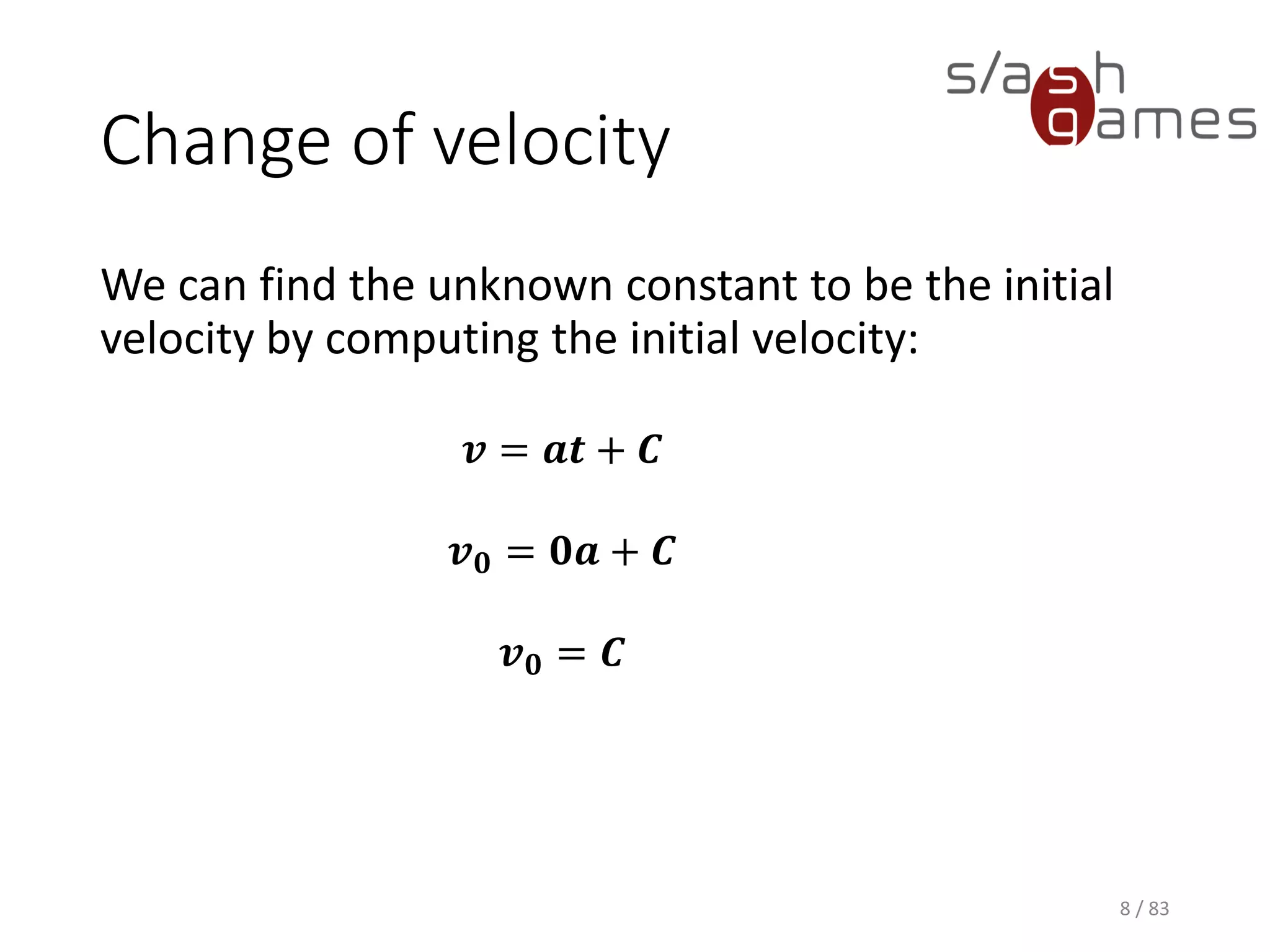
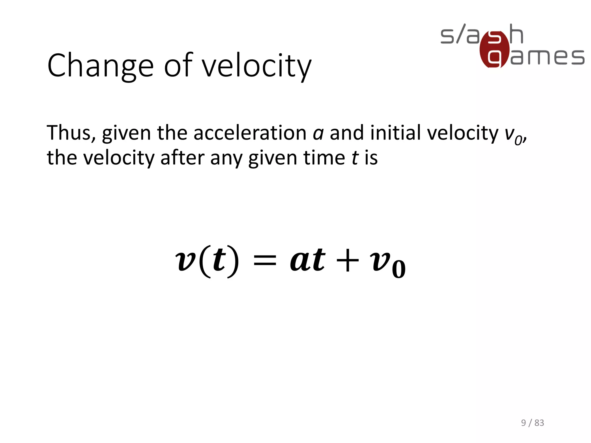
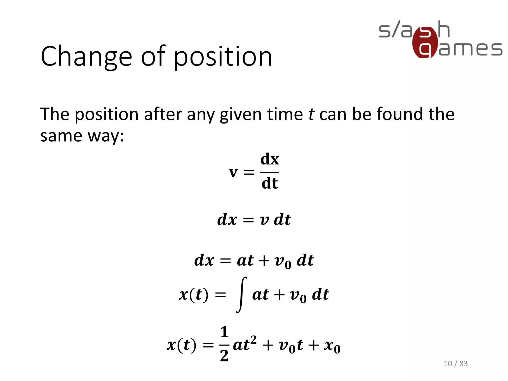
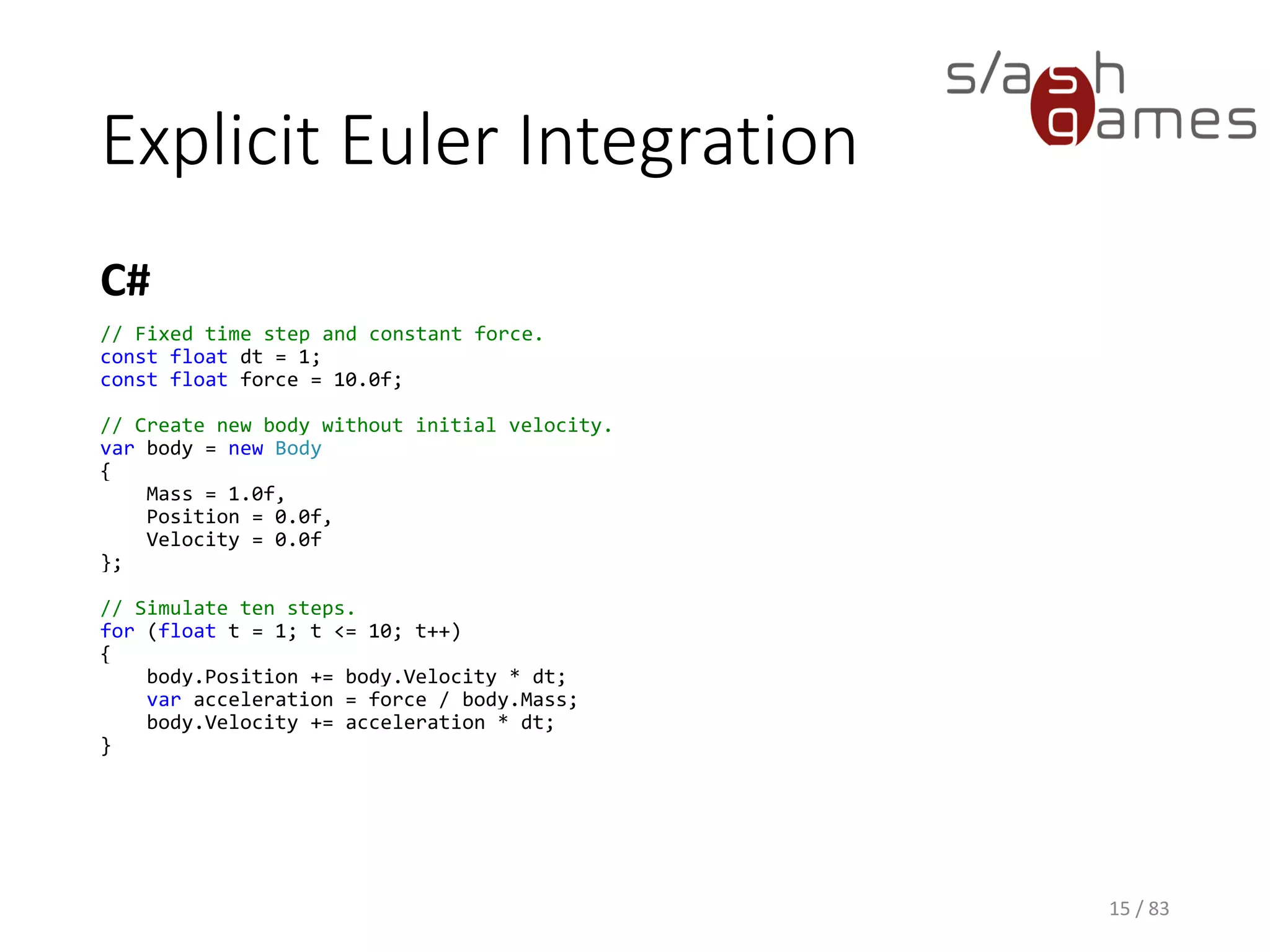
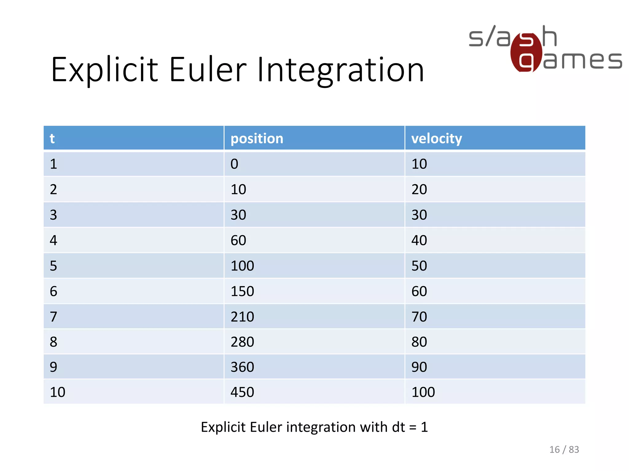

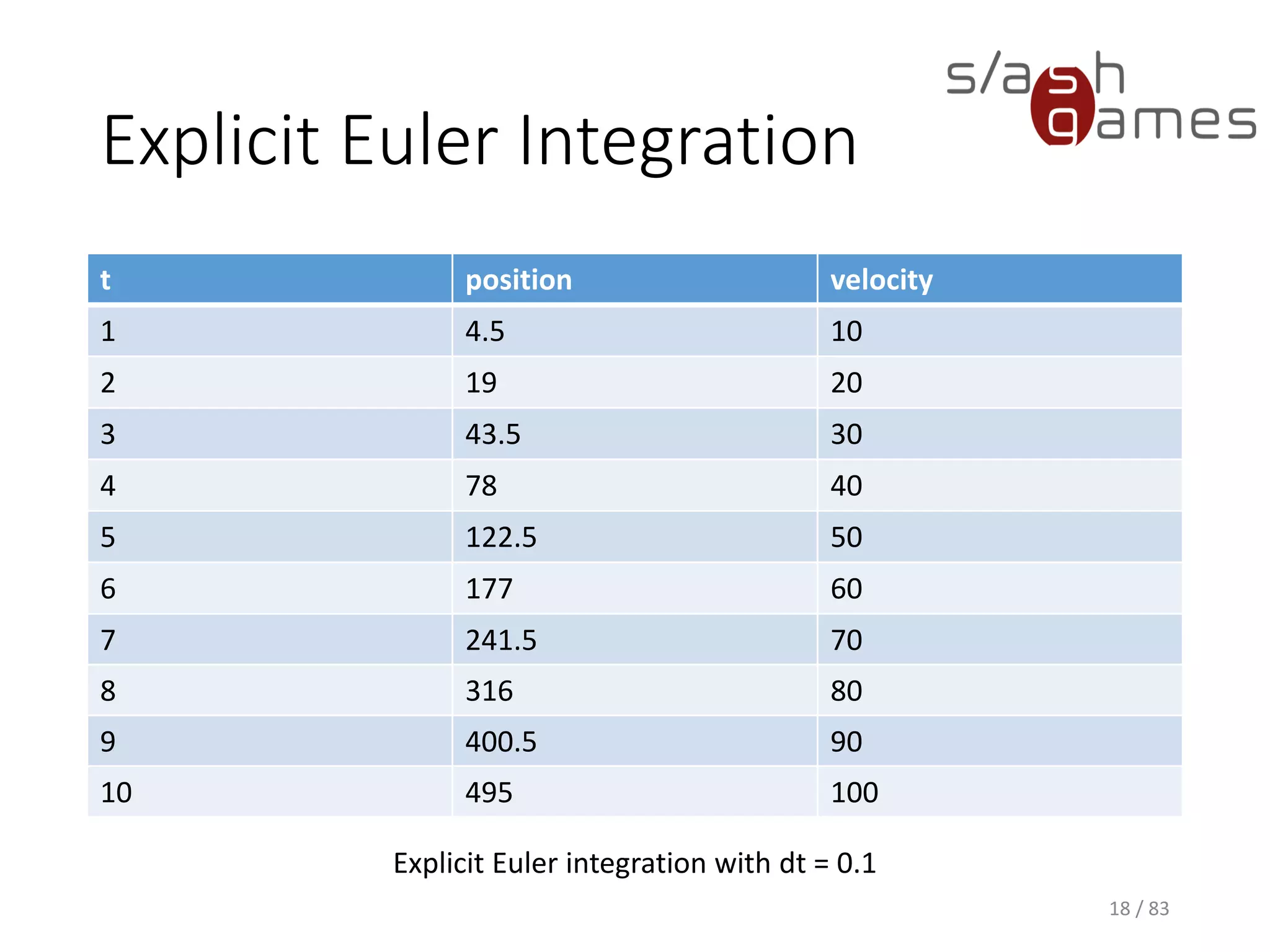
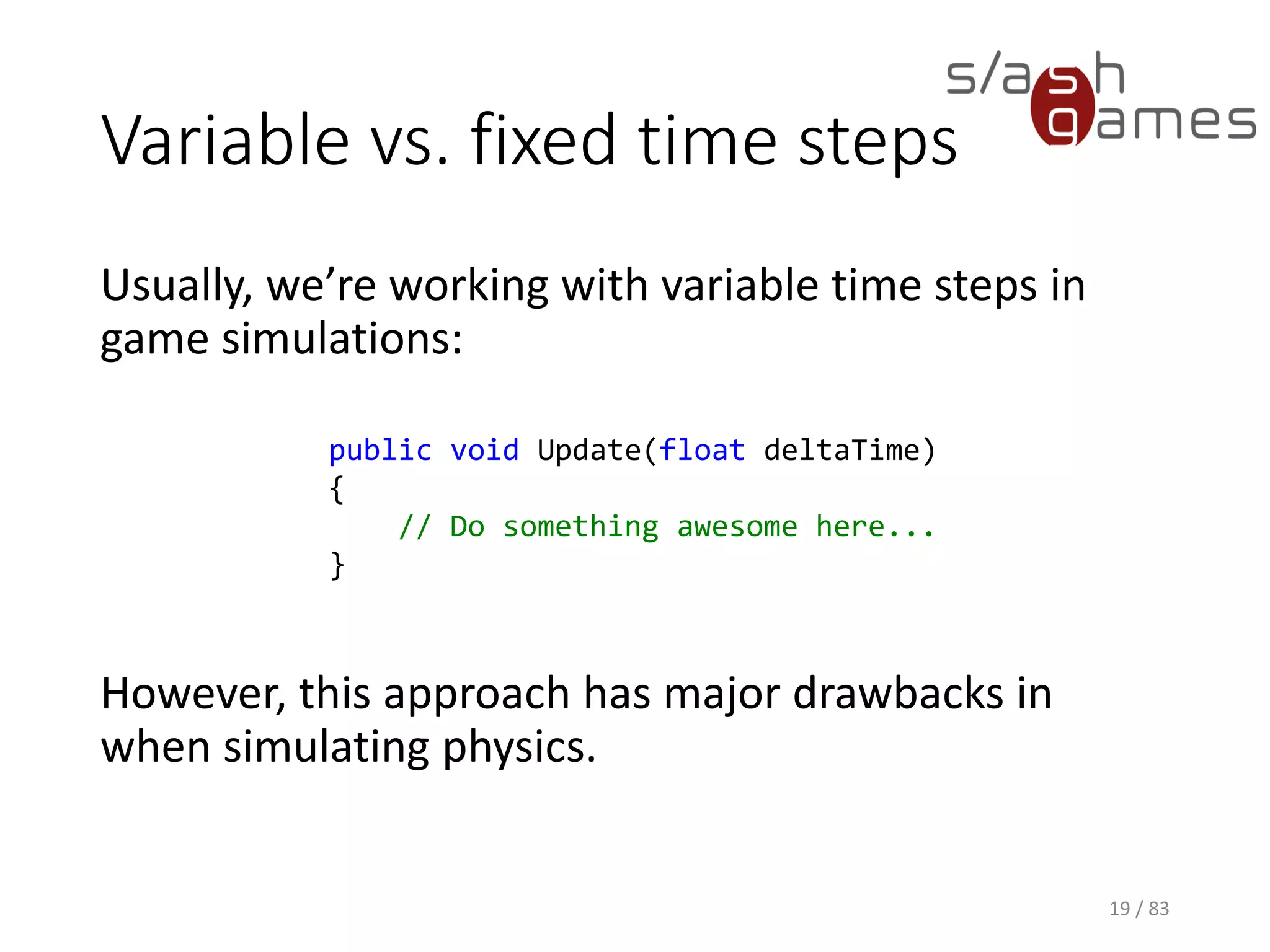
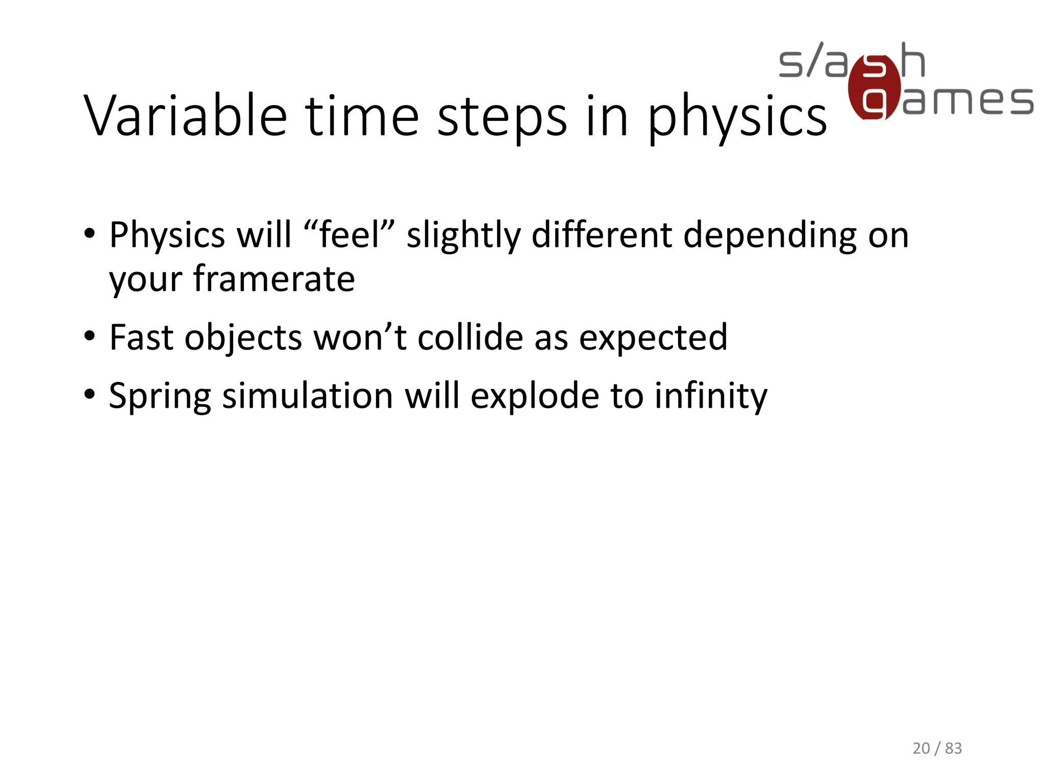
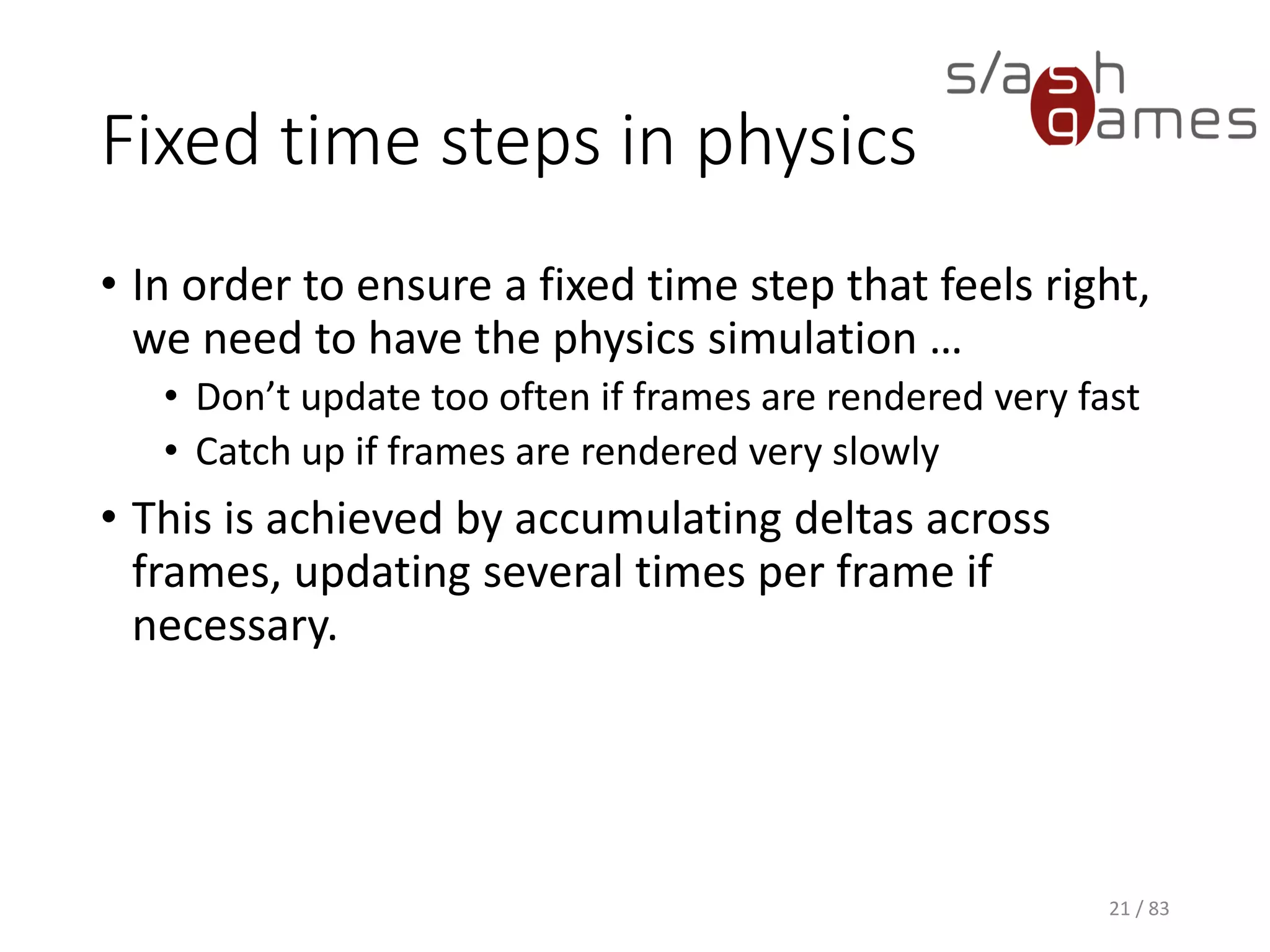
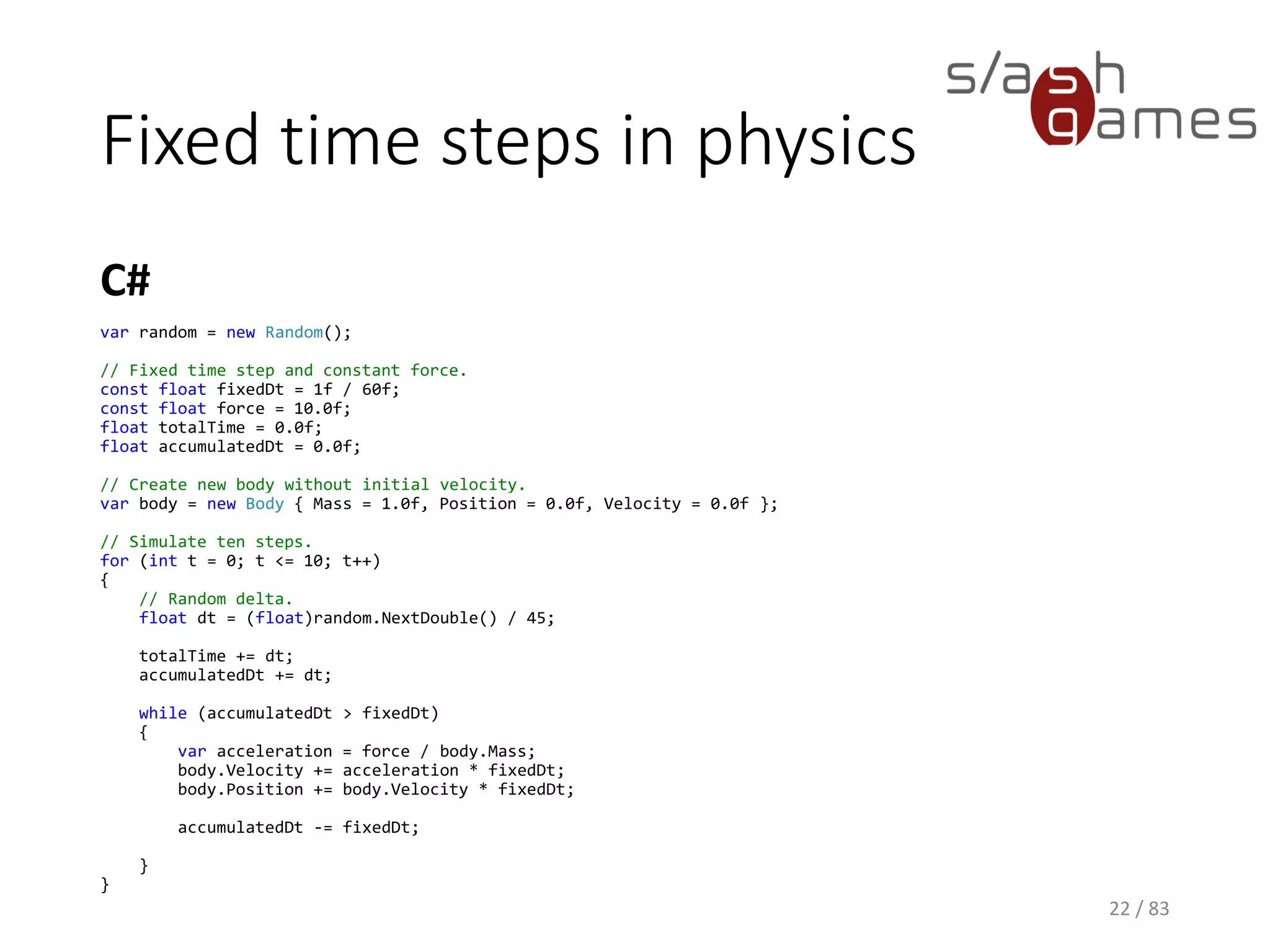
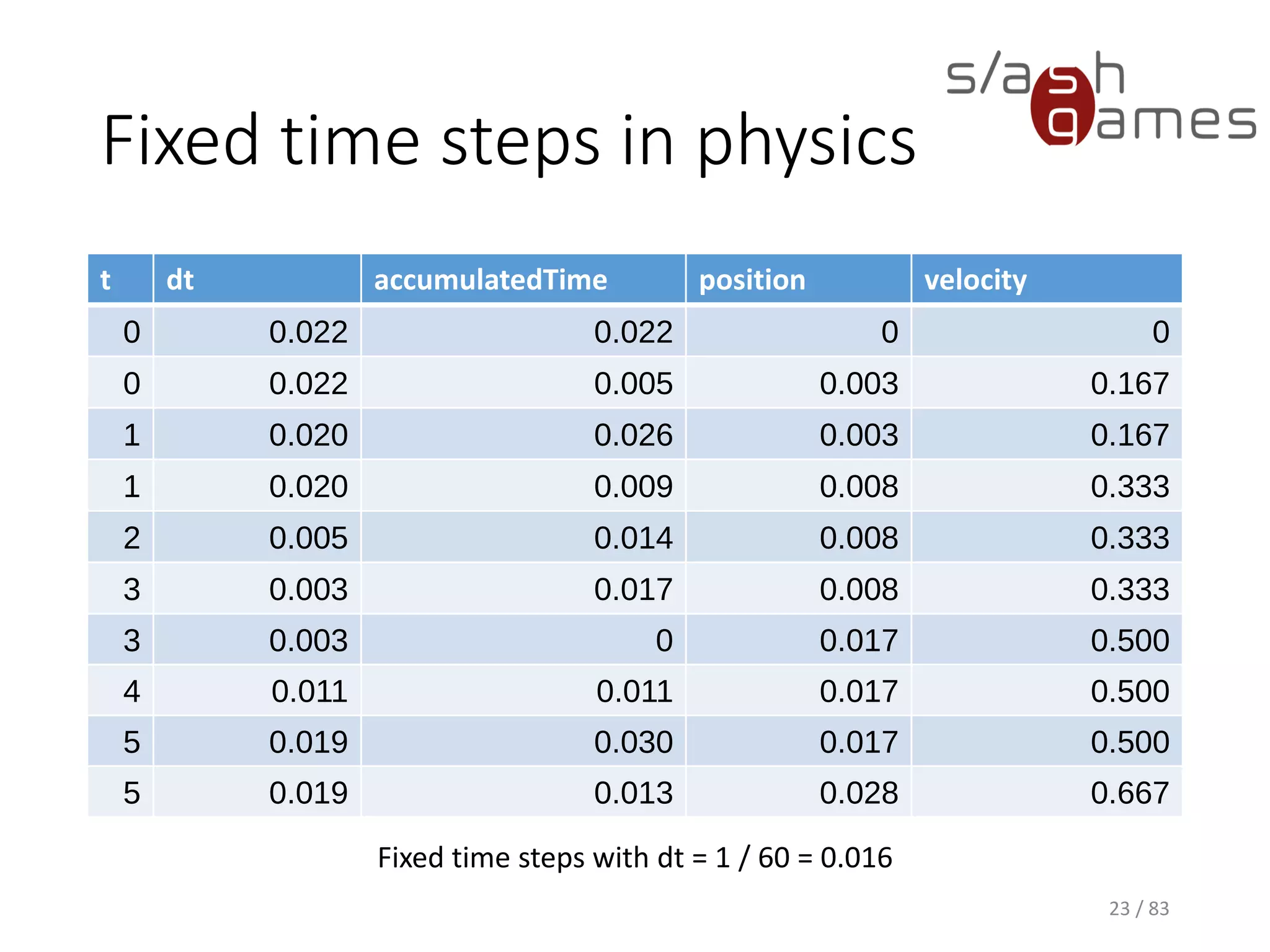


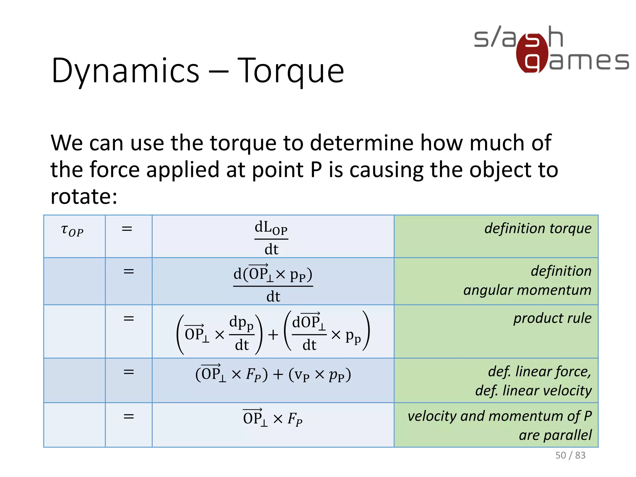
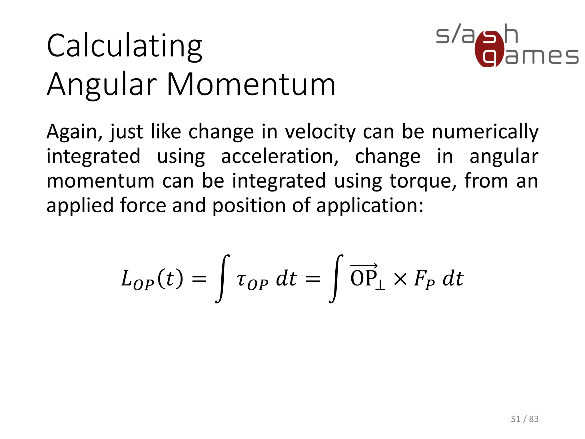
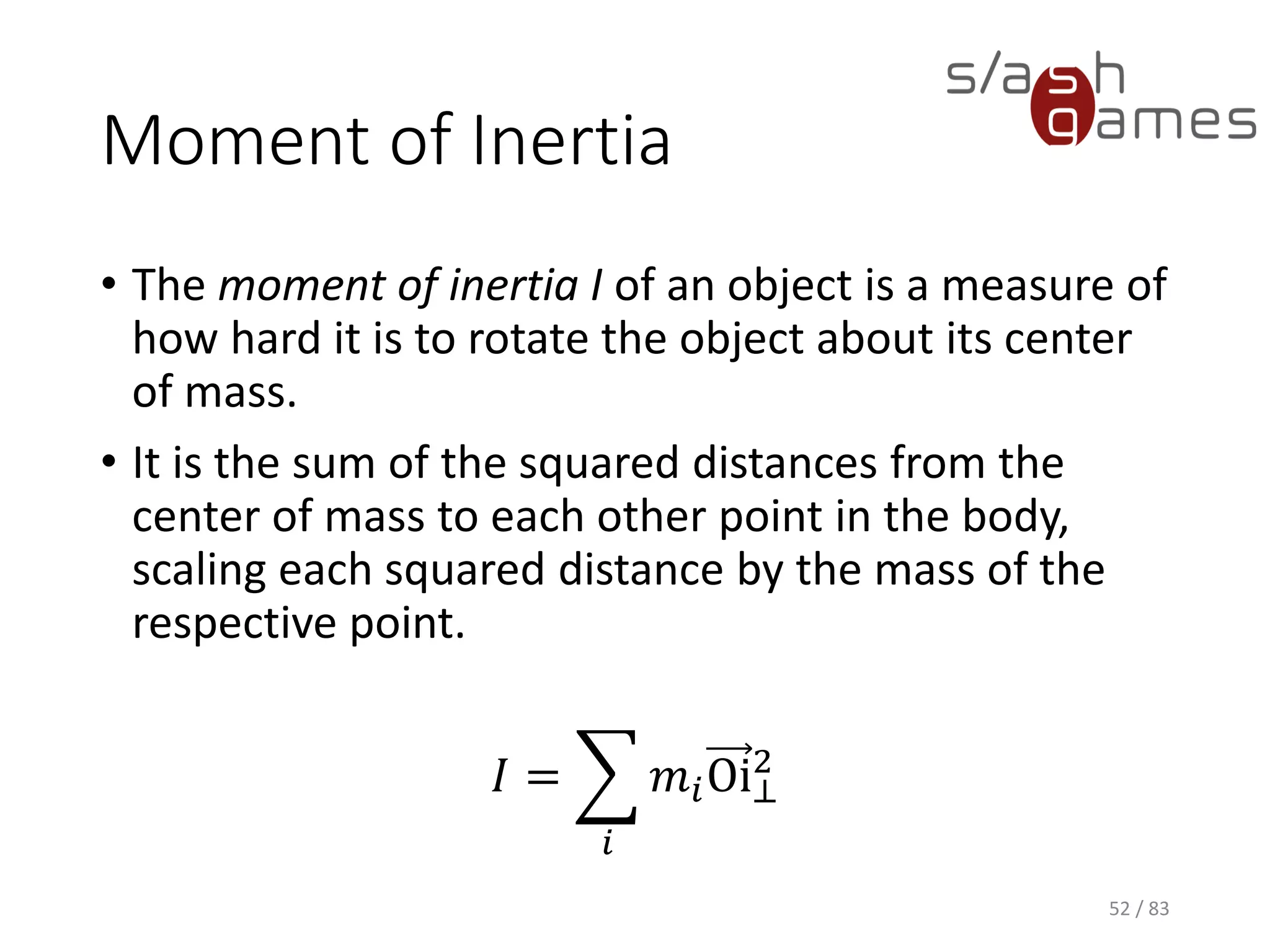
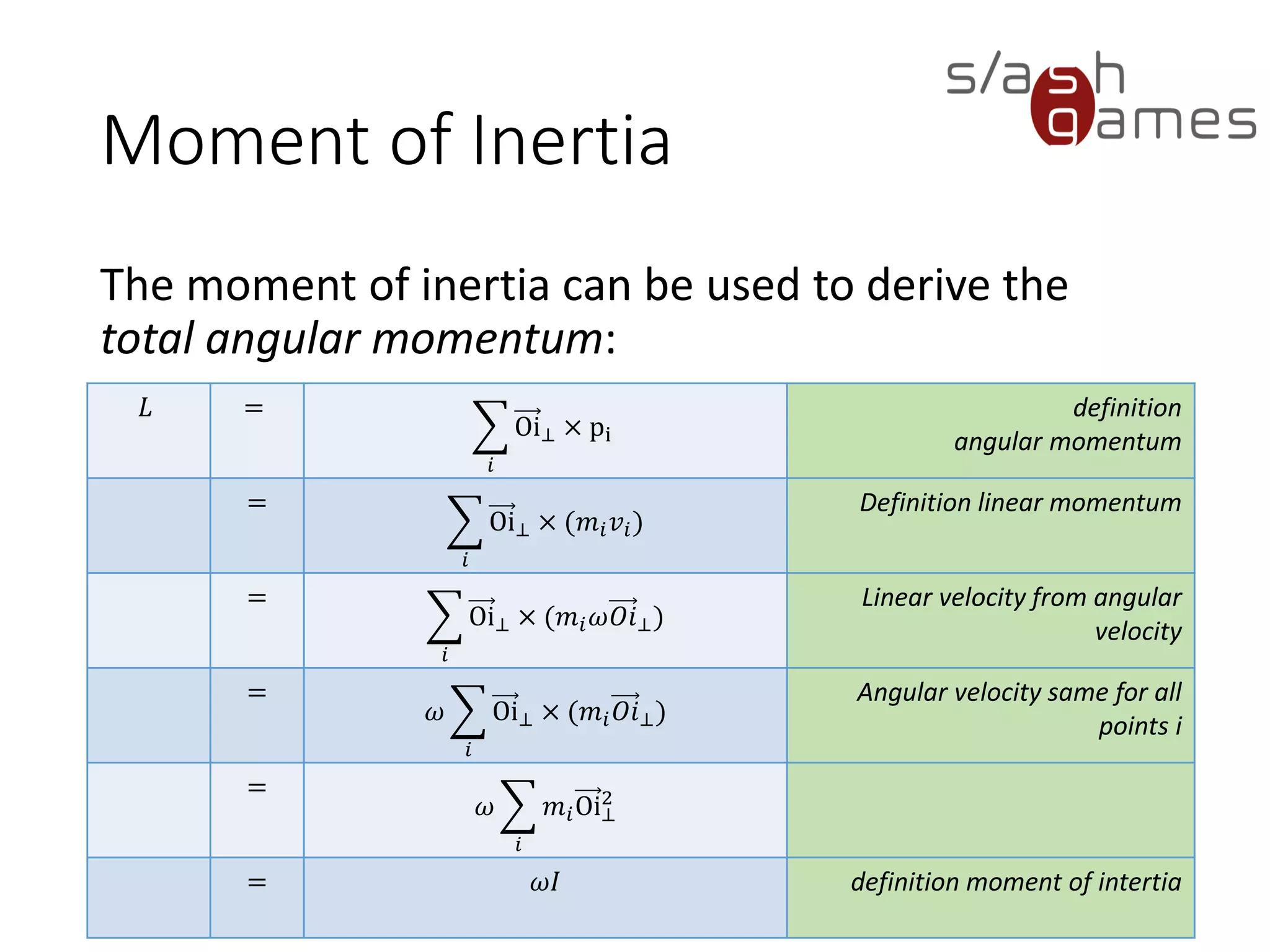


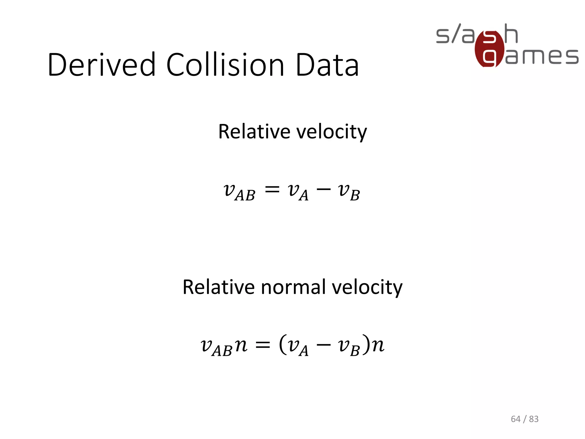
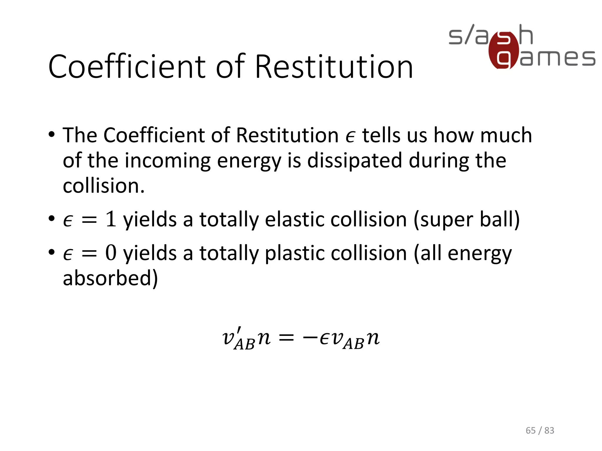
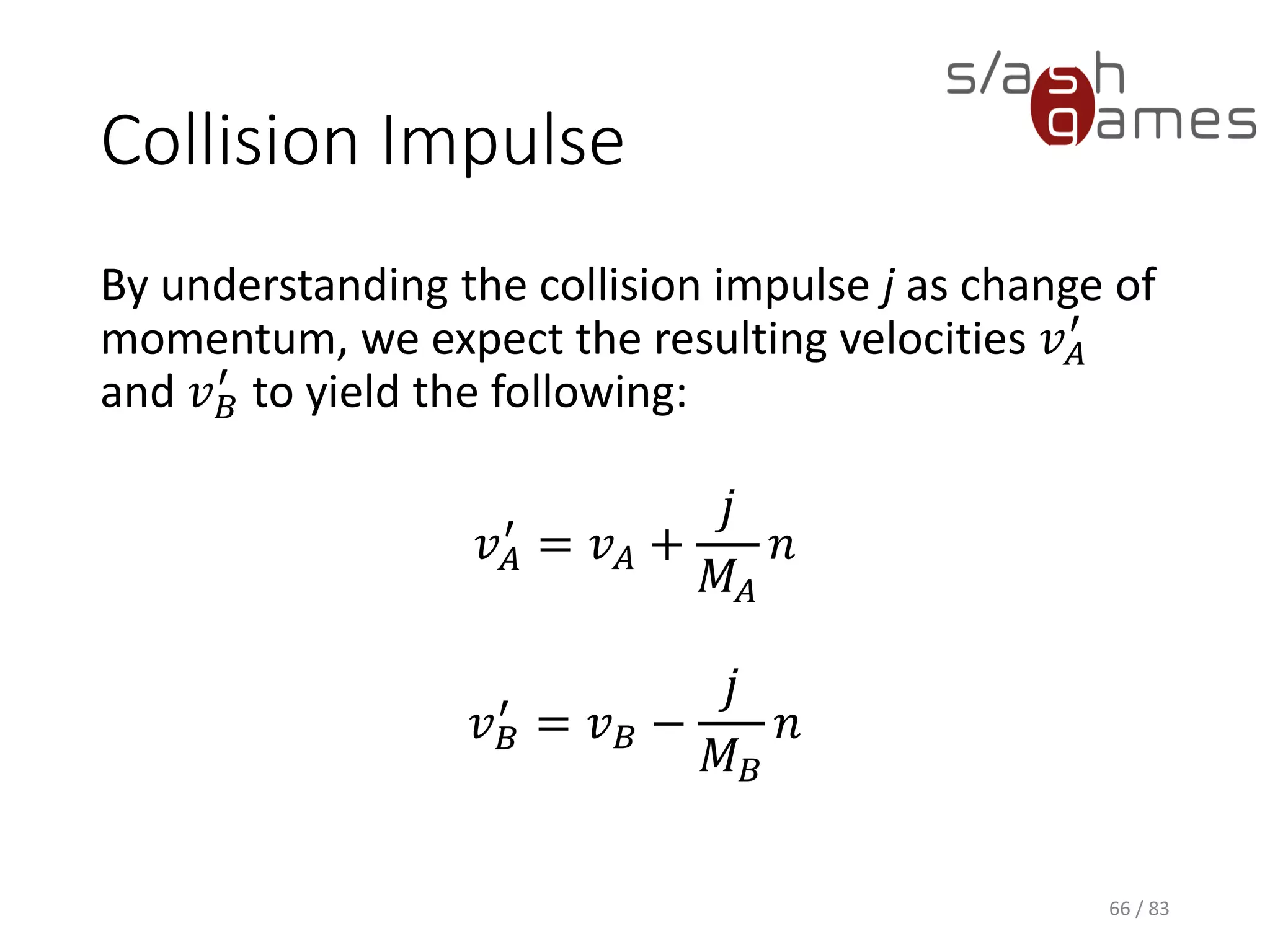
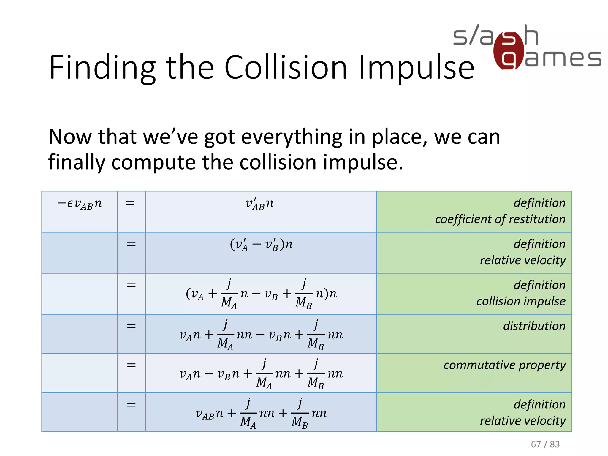
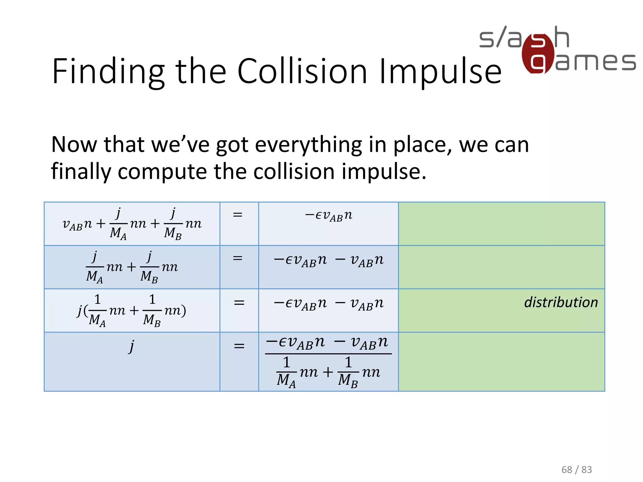
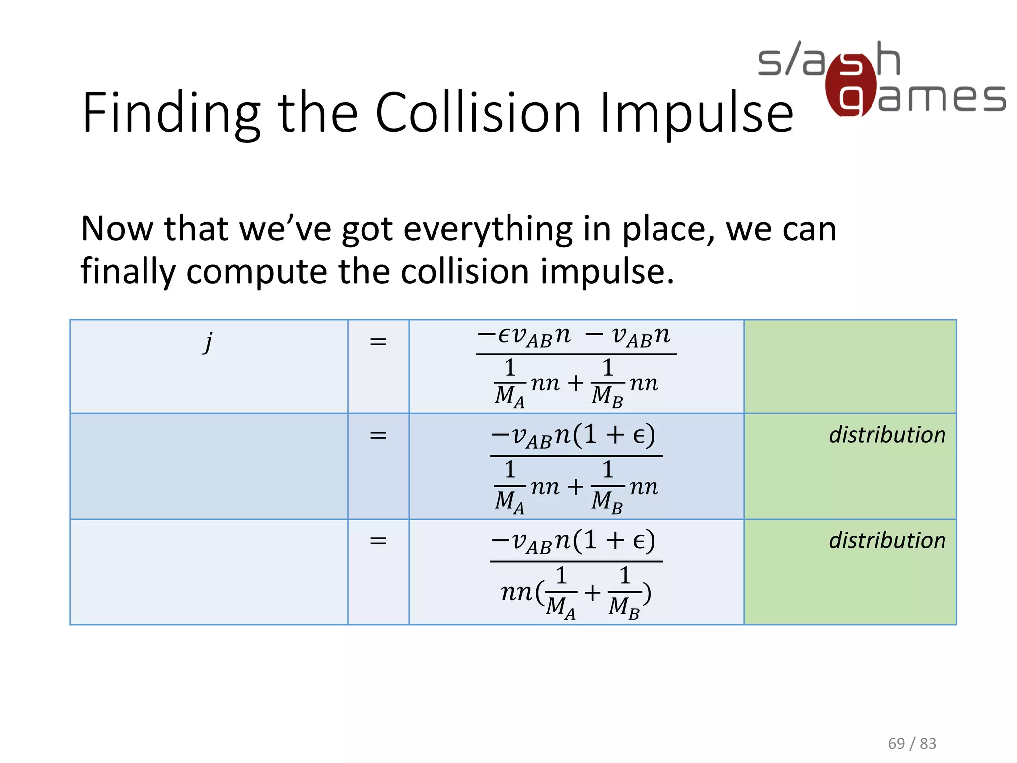
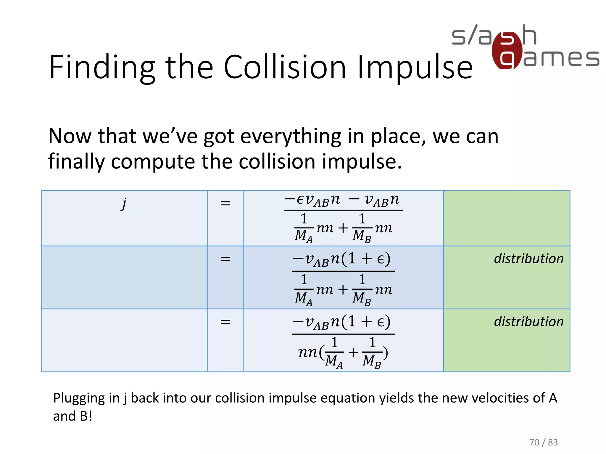
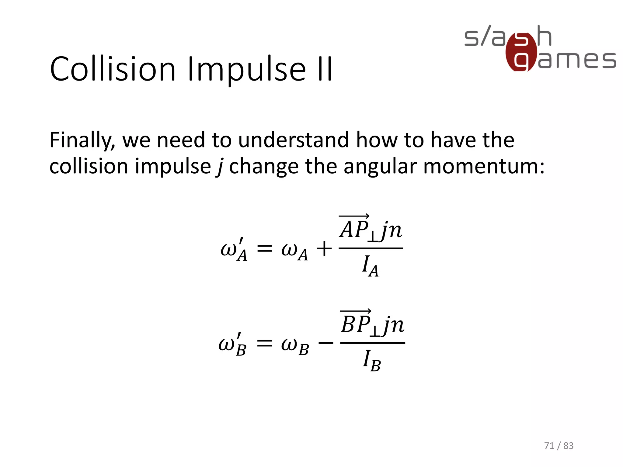
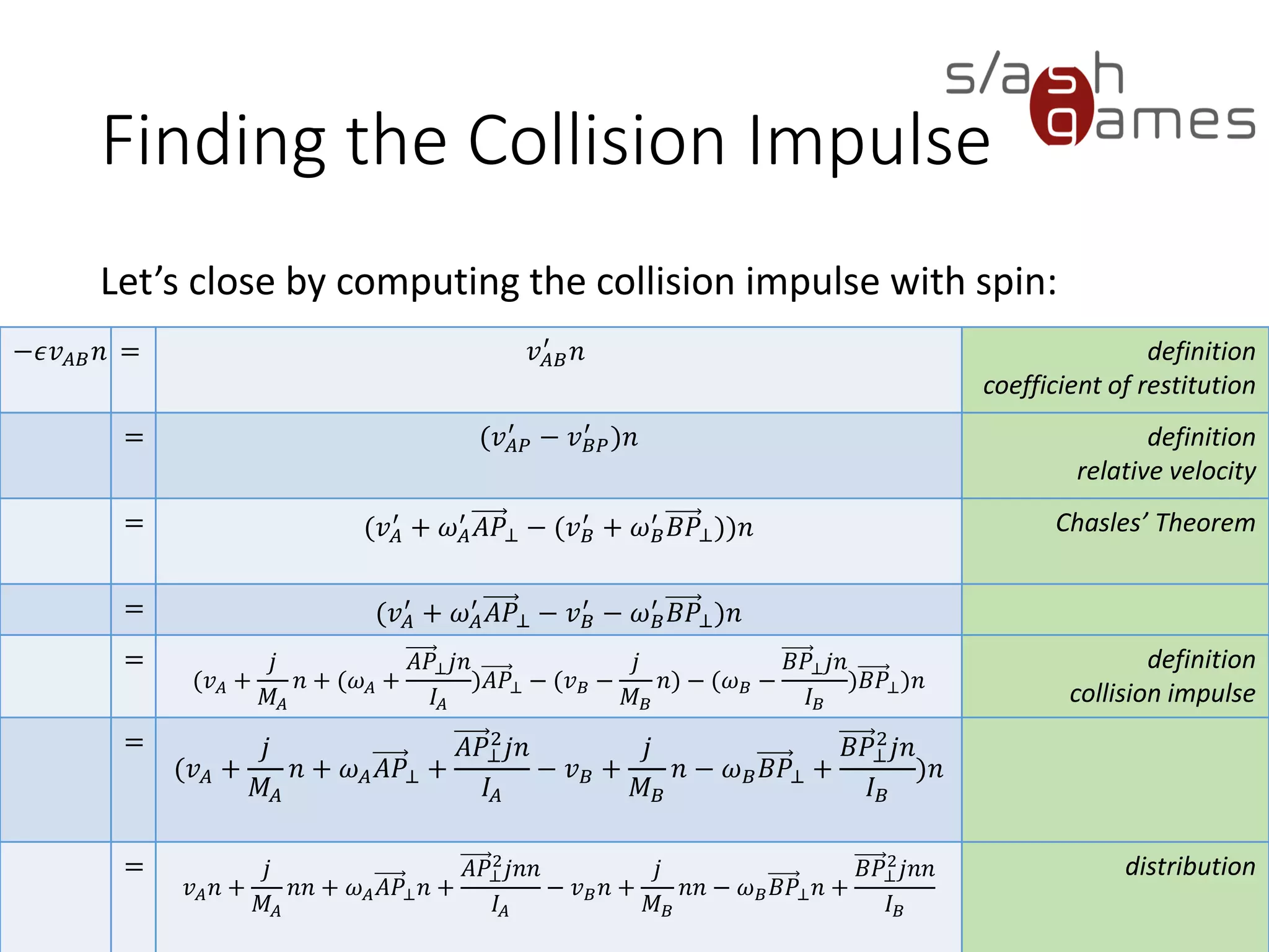
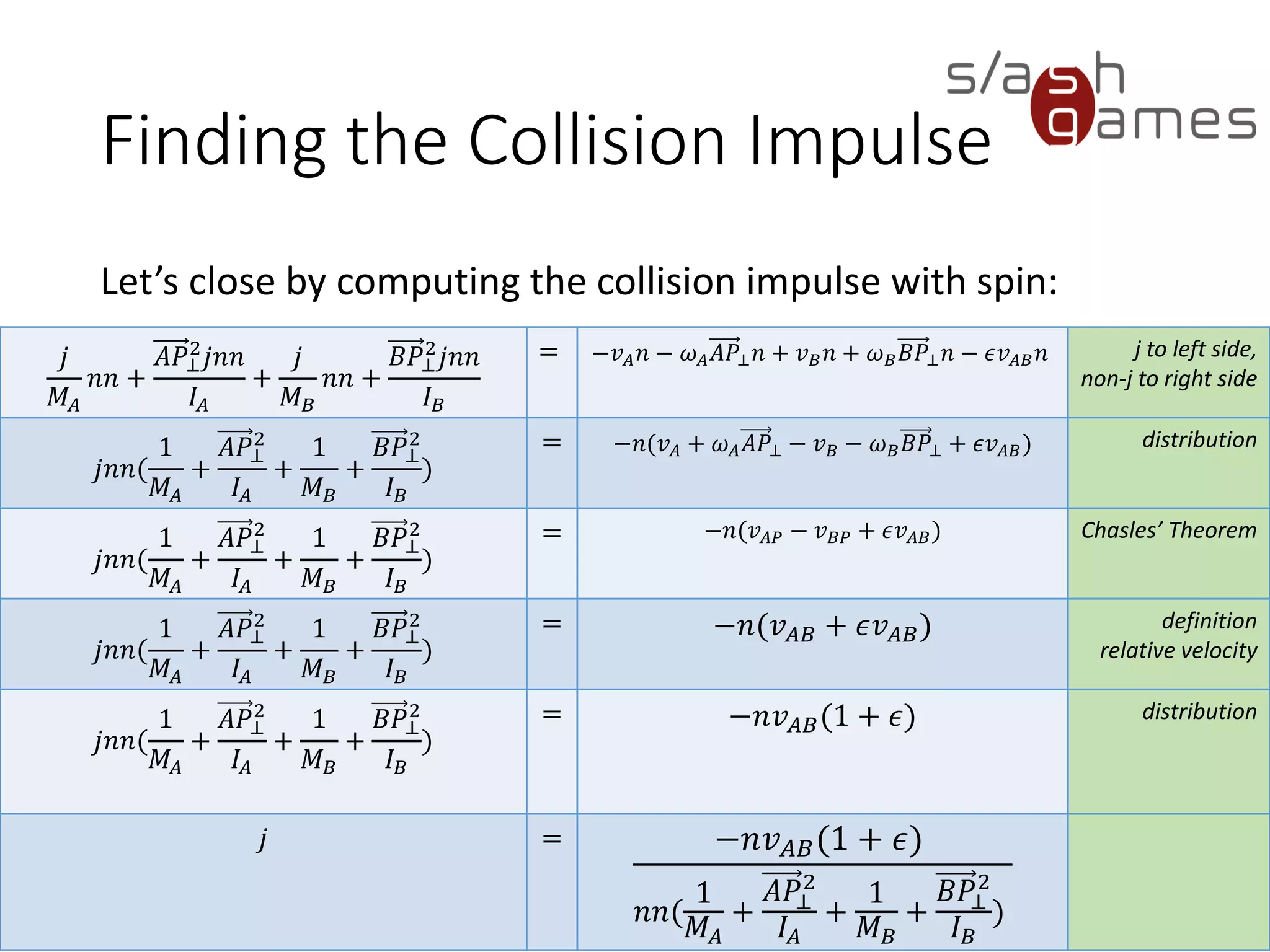


This document discusses the fundamentals of physics in game programming, focusing on kinematics, dynamics, rigid body collisions, and numerical integration methods. It covers concepts such as motion, forces, velocity, and the importance of using fixed time steps for accurate physics simulations. The document also elaborates on the properties of rigid bodies, collision response, and the calculations related to center of mass and moments of inertia.


![[IGC 2017] 펄어비스 민경인 - Mmorpg를 위한 voxel 기반 네비게이션 라이브러리 개발기](https://cdn.slidesharecdn.com/ss_thumbnails/mmorpgvoxel-170905061528-thumbnail.jpg?width=600ounds&width=560&fit=bounds)
![NDC 2015 이광영 [야생의 땅: 듀랑고] 전투 시스템 개발 일지](https://cdn.slidesharecdn.com/ss_thumbnails/ndc2015-kwangyoung-150522112340-lva1-app6891-thumbnail.jpg?width=600ounds&width=560&fit=bounds)


![[KGC 2012]Boost.asio를 이용한 네트웍 프로그래밍](https://cdn.slidesharecdn.com/ss_thumbnails/kgc2012boost-asio-121011023325-phpapp02-thumbnail.jpg?width=600ounds&width=560&fit=bounds)


